Circuit Simulation using Matrix Exponential Method

Shih-Hung Weng, Quan Chen and Chung-Kuan ChengCSE Department, UC San Diego, CA 92130

Contact: ckcheng@ucsd.edu

1

Outline

• Introduction• Computation of Matrix Exponential Method

– Krylov Subspace Approximation– Adaptive Time Step Control

• Experimental Results• Conclusions

2

Circuit Simulation

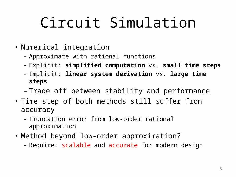
• Numerical integration– Approximate with rational functions– Explicit: simplified computation vs. small time steps– Implicit: linear system derivation vs. large time steps

– Trade off between stability and performance• Time step of both methods still suffer from accuracy

– Truncation error from low-order rational approximation

• Method beyond low-order approximation?– Require: scalable and accurate for modern design

3

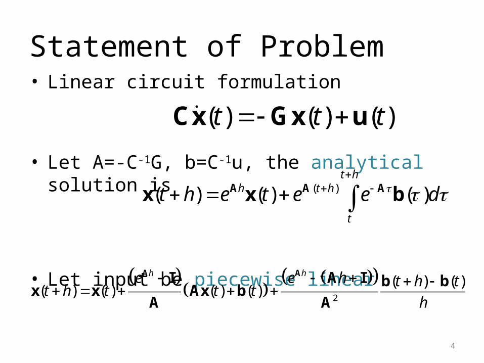
Statement of Problem• Linear circuit formulation

• Let A=-C-1G, b=C-1u, the analytical solution is

• Let input be piecewise linear

4

( ) ( ) ( )t t t Cx Gx u

( )( ) ( ) ( )t h

h t h

t

t h e t e e d

A A Ax x b

2

( ) ( )( ) ( ) ( ) ( )

h he e h t h tt h t t t

h

A AI A I b bx x Ax b

A A

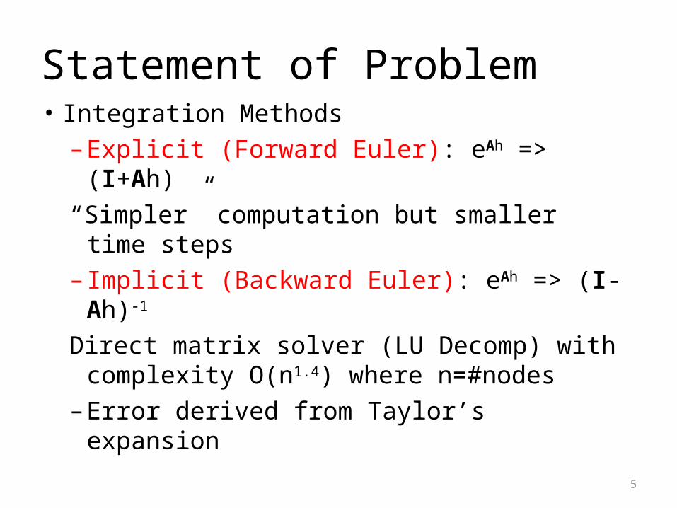
Statement of Problem• Integration Methods

– Explicit (Forward Euler): eAh => (I+Ah) “Simpler” computation but smaller time

steps– Implicit (Backward Euler): eAh => (I-Ah)-1

Direct matrix solver (LU Decomp) with complexity O(n1.4) where n=#nodes

– Error derived from Taylor’s expansion

5

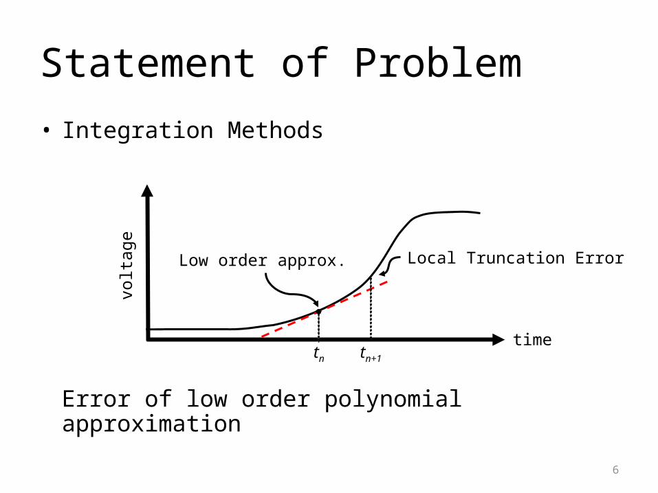
Statement of Problem

• Integration Methods

Error of low order polynomial approximation

6

volta

ge

timetn tn+1

Low order approx. Local Truncation Error

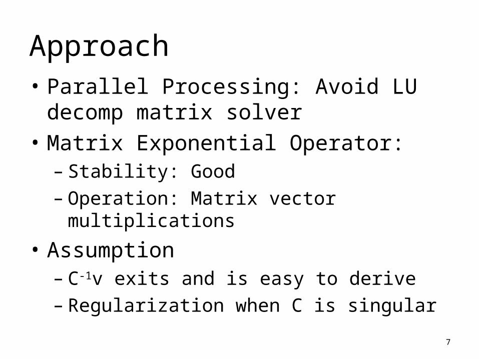
Approach• Parallel Processing: Avoid LU decomp matrix

solver• Matrix Exponential Operator:

– Stability: Good– Operation: Matrix vector multiplications

• Assumption– C-1v exits and is easy to derive– Regularization when C is singular

7

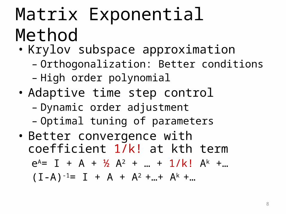
Matrix Exponential Method• Krylov subspace approximation

– Orthogonalization: Better conditions– High order polynomial

• Adaptive time step control– Dynamic order adjustment– Optimal tuning of parameters

• Better convergence with coefficient 1/k! at kth term eA= I + A + ½ A2 + … + 1/k! Ak +…(I-A)-1= I + A + A2 +…+ Ak +…

8

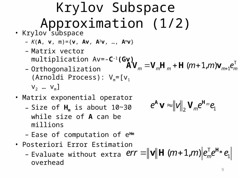
Krylov Subspace Approximation (1/2)• Krylov subspace

– K(A, v, m)={v, Av, A2v, …, Amv}

– Matrix vector multiplication Av=-C-1(Gv)

– Orthogonalization (Arnoldi Process): Vm=[v1 v2 … vm]

• Matrix exponential operator– Size of Hm is about 10~30 while

size of A can be millions– Ease of computation of eHm

• Posteriori Error Estimation – Evaluate without extra

overhead9

1( 1, )m m m m mm m e AV V H H v T

12m

me v e e HAv V

1( 1, ) merr m m e e e mHv H T

RC circuit of 500 nodes, random cap ranges 1e-11~1e-16, h = 1e-13

Krylov Subspace Approximation (2/2)

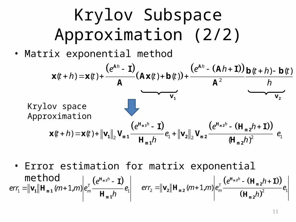
• Matrix exponential method

• Error estimation for matrix exponential method

11

1 1( 1, )

h

m

eerr m m e e

h

m1H

1 m1m1

Iv H

HT

2 12( 1, )h

m

e herr m m e e

h

m2Hm2

2 m2

m2

H Iv H

HT

1 122 2

( ) ( )( )

h he e ht h t e e

h h

m1 m2H Hm2

1 m1 2 m2m1 m2

I H Ix x v V v V

H H

2

( ) ( )( ) ( ) ( ) ( )

h he e h t h tt h t t t

h

A AI A I b bx x Ax b

A A

Krylov space Approximation

v1 v2

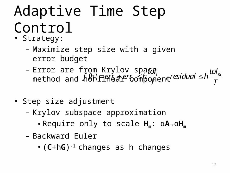
Adaptive Time Step Control• Strategy:

– Maximize step size with a given error budget– Error are from Krylov space method and

nonlinear component

• Step size adjustment– Krylov subspace approximation

• Require only to scale Hm: αA→αHm

– Backward Euler• (C+hG)-1 changes as h changes

12

1 2( ) , l nltol tolf h err err h residual h

T T

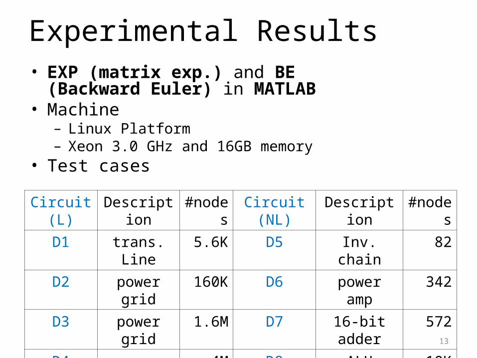
Experimental Results• EXP (matrix exp.) and BE (Backward Euler) in

MATLAB• Machine

– Linux Platform – Xeon 3.0 GHz and 16GB memory

• Test cases

13

Circuit (L) Description #nodes Circuit (NL) Description #nodes

D1 trans. Line 5.6K D5 Inv. chain 82

D2 power grid 160K D6 power amp 342

D3 power grid 1.6M D7 16-bit adder 572

D4 power grid 4M D8 ALU 10K

14

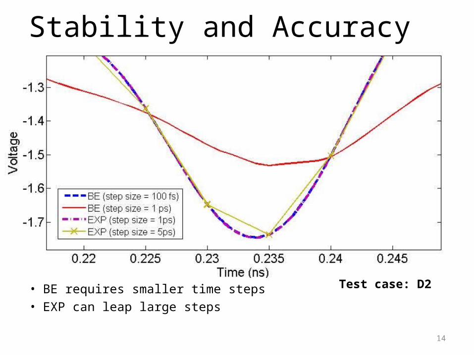
Test case: D2• BE requires smaller time steps• EXP can leap large steps

Stability and Accuracy

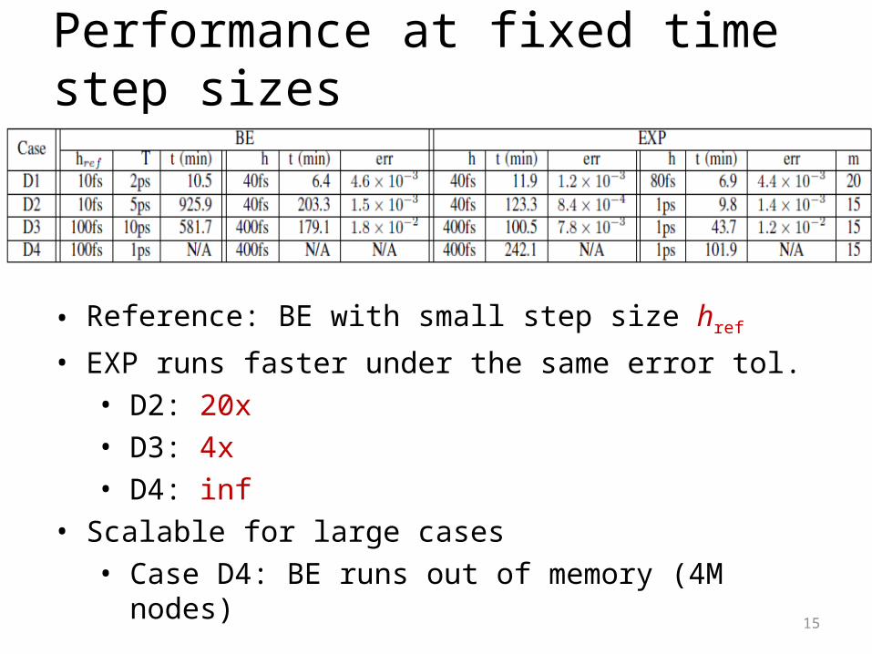
Performance at fixed time step sizes

15

• Reference: BE with small step size href

• EXP runs faster under the same error tol.• D2: 20x• D3: 4x• D4: inf

• Scalable for large cases• Case D4: BE runs out of memory (4M nodes)

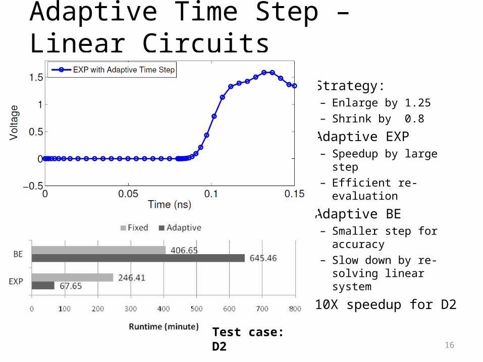
Adaptive Time Step – Linear Circuits

• Strategy:– Enlarge by 1.25– Shrink by 0.8

• Adaptive EXP– Speedup by large step– Efficient re-evaluation

• Adaptive BE– Smaller step for

accuracy– Slow down by re-

solving linear system

• 10X speedup for D2

16

Test case: D2

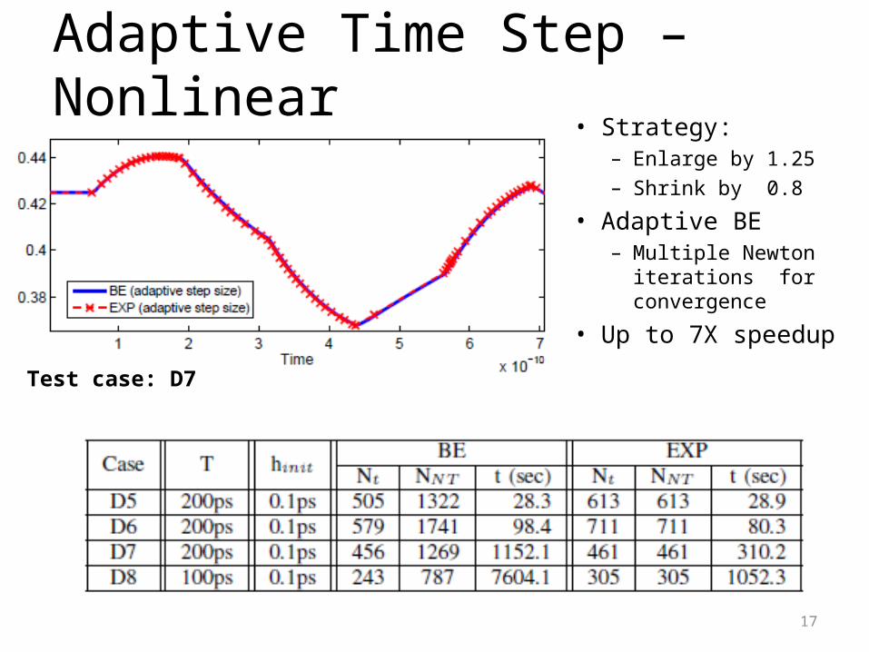
Adaptive Time Step – Nonlinear • Strategy:

– Enlarge by 1.25– Shrink by 0.8

• Adaptive BE– Multiple Newton

iterations for convergence

• Up to 7X speedup

17

Test case: D7

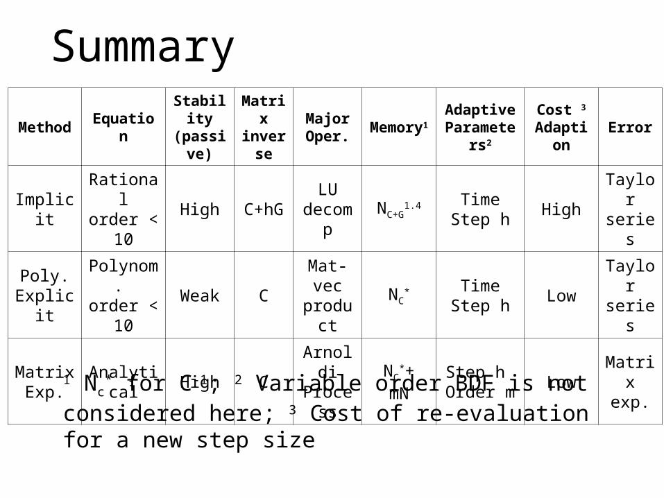
Method Equation Stability(passive)

Matrix inverse

MajorOper. Memory1 Adaptive

Parameters2

Cost 3

Adaption Error

Implicit Rationalorder < 10 High C+hG LU

decompNC+G

1.4 TimeStep h High Taylor

series

Poly. Explicit

Polynom. order < 10 Weak C Mat-vec

productNC

* TimeStep h Low Taylor

series

Matrix Exp. Analytical High C Arnoldi

ProcessNC

*+mN

Step h Order m Low Matrix

exp.

1 Nc* for C-1; 2 Variable order BDF is not considered

here; 3 Cost of re-evaluation for a new step size

Summary

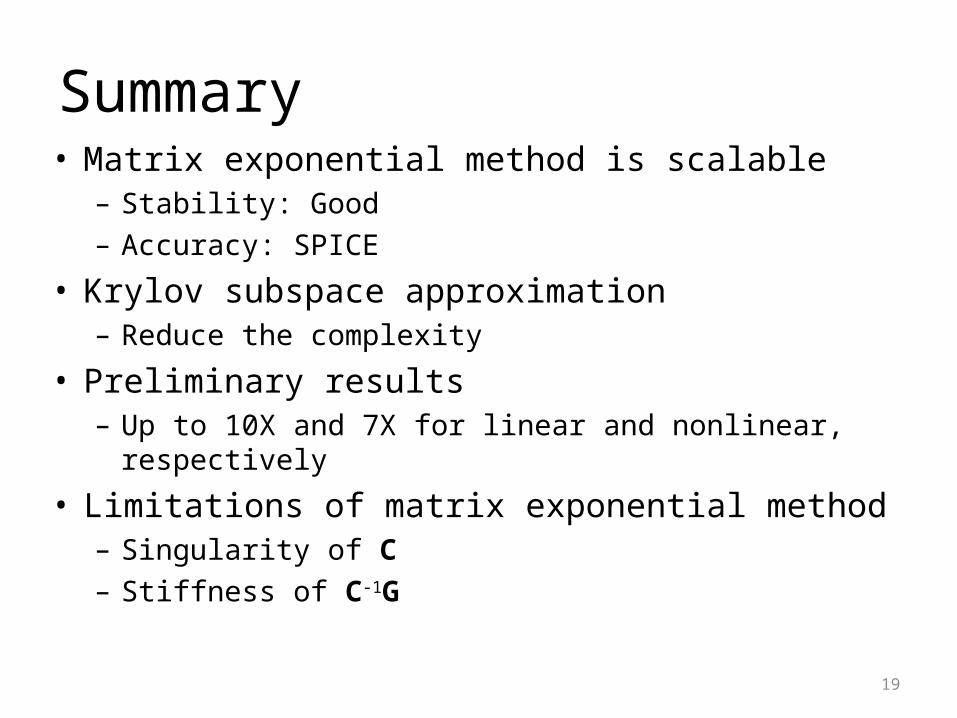
Summary• Matrix exponential method is scalable

– Stability: Good– Accuracy: SPICE

• Krylov subspace approximation– Reduce the complexity

• Preliminary results – Up to 10X and 7X for linear and nonlinear, respectively

• Limitations of matrix exponential method– Singularity of C– Stiffness of C-1G

19

Future Works• Scalable Parallel Processing

– Integration– Matrix Operations

• Applications– Power Ground Network Analysis– Substrate Noises– Memory Analysis– Tera Hertz Circuit Simulation

20

Thank You!

21