CHEMICAL ENGINEERING COMPUTATION

SKKK 2133

SYED ANUAR FAUA’AD B. SYED MUHAMMADDept. of Bioprocess and PolymerEngineering, Faculty of Chemical and Energy Engineering.

UTM Skudai, JohorN01-257

syed@utm.my

WORLDVIEW KNOWLEDGE,

FRAMEWORK CIVILIZATION & THE

DEVELOPMENT OF A HOLISTIC

PERSONALITY: COMPARATIVE

PERSPECTIVE

11-12 SEPT 2013

PROF. DR. WAN MOHD NOR WAN DAUD

Founder Director

Advance Studies on Islam, Science and Civilisation (CASIS),

UTM Skudai.

• CHAPTER 1 – INTRODUCTION to NUMERICAL METHODS

• CHAPTER 2 – APPROXIMATIONS & ERRORS

• CHAPTER 3 – PART I : MATLAB FUNDAMENTALS

– PART II : PROGRAMMING WITH MATLAB

• CHAPTER 4 – ROOTS OF EQUATIONS

• CHAPTER 5 – LINEAR ALGEBRAIC EQUATIONS

• CHAPTER 6 – CURVE FITTING

• CHAPTER 7 – NUMERICAL DIFFERENTIATION

• CHAPTER 8 – NUMERICAL INTEGRATION

• CHAPTER 9 – ORDINARY DIFFERENTIAL EQUATIONS

(ODE)

COURSE OUTLINES

CHAPTER 1

INTRODUCTION TO

NUMERICAL METHODS (NMs)

Chapter 1 : TOPIC COVERS

(INTRODUCTION to NMs)

• Computers and Numerical Methods

• Advantages (NMs) and Disadvantages

(analytical/exact solution)

• Role of Numerical Methods in Engineering

LEARNING OUTCOMES

INTRODUCTION

It is expected that students will be able to:

• Recognize the difference between analytical and

numerical solutions

• Describe how conservation laws are employed to

develop mathematical models of physical systems

• Identify the advantages and disadvantages of learning

numerical methods

Numerical methods

Techniques by which mathematical

problems are formulated so that

they can be solved with

arithmetic/reckoning/calculation

operations – i.e involve large

numbers of calculation

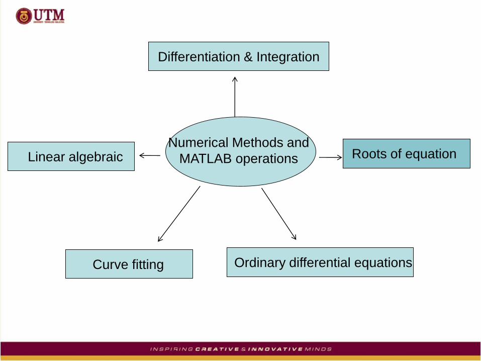
Numerical Methods and

MATLAB operationsLinear algebraic

Differentiation & Integration

Curve fitting Ordinary differential equations

Roots of equation

Engineers approached to solve problems during

pre-computer era:

a. Using analytical or exact methods – only for a

simple linear models or simple geometry and

low dimensionality.

b. Graphical solutions – to solve complex

problems but the results are not precise & can

be described using three or less dimensions.

c. Calculators approaches – to implement NM

manually. Although perfectly adequate for

solving complex problems, manual calculations

are slow, tedious & consistent results are

indefinable/elusive/hard to define.

Nowadays, computers & NMs provide an

alternative for complicated calculations.

Since late 1940s digital computers has lead

in the use & development of NMs.

There are several advantages of study NMs:

a. Powerful-solving tools – capable of handling

large systems of equations, nonlinearities and

complicated geometries that uncommon in

engineering practice & impossible to solve

analytically.

b. An efficient vehicle for learning to use

computers – an efficient way to learn

programming as NMs are the important part

for implementation on computers.

c. Reinforce/support understanding of

mathematics – function of NM is to reduce

high mathematics to basic reckoning/arithematic/calculation

operations.

Mathematical Modeling and

Engineering Problem solving

• Requires understanding of engineering systems:

– By observation and experiment

– Theoretical analysis and generalization

• Computers are great tools, however, without

fundamental understanding of engineering

problems, they will be useless.

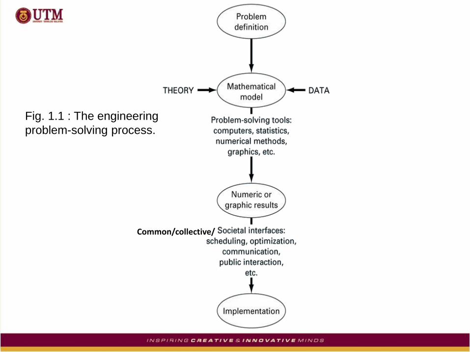
Fig. 1.1 : The engineering

problem-solving process.

Common/collective/

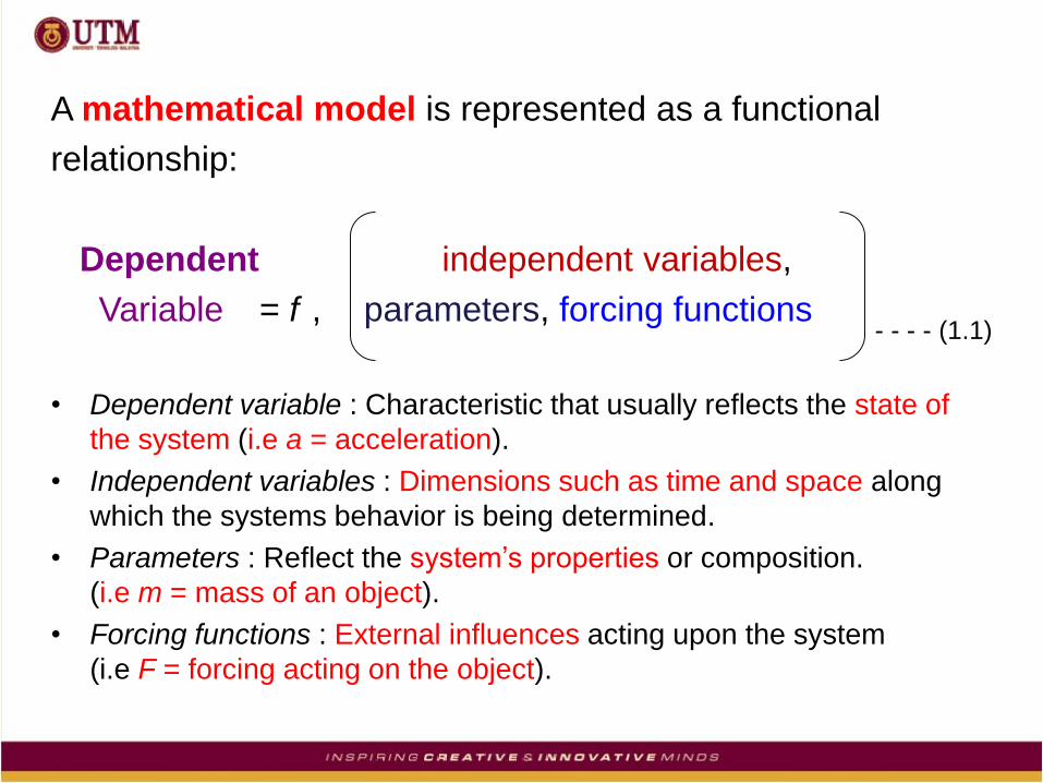
A mathematical model is represented as a functional

relationship:

Dependent independent variables,

Variable = f , parameters, forcing functions

• Dependent variable : Characteristic that usually reflects the state of

the system (i.e a = acceleration).

• Independent variables : Dimensions such as time and space along

which the systems behavior is being determined.

• Parameters : Reflect the system’s properties or composition.

(i.e m = mass of an object).

• Forcing functions : External influences acting upon the system

(i.e F = forcing acting on the object).

- - - - (1.1)

Equation (1.1) can be ranged from a simple

mathematical /algebraic/numerical relationship to large

complicated sets of differential equations.

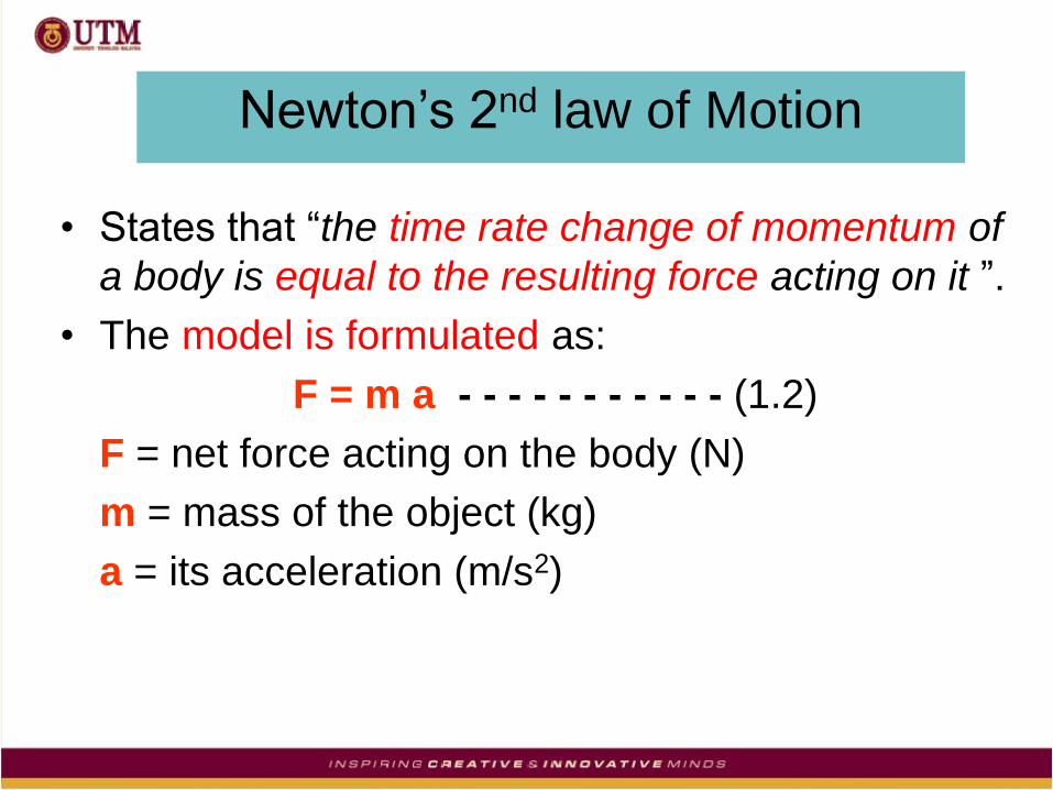
Newton’s 2nd law of Motion

• States that “the time rate change of momentum of

a body is equal to the resulting force acting on it ”.

• The model is formulated as:

F = m a - - - - - - - - - - - (1.2)

F = net force acting on the body (N)

m = mass of the object (kg)

a = its acceleration (m/s2)

Equation (1.2) can be written as:

a = F / m

simple algebraic equation that can be solved

analytically.

a = dependent variable (or system’s behavior)

F = forcing function

m = parameter (or property of system)

No independent variable because we are not yet predicting

how acceleration varies in time or space.

Equation (1.2) has characteristics as typical of

mathematical models:

a. Describes a physical system or process in

mathematical terms.

b. Represents an idealization & simplification of

reality – by ignores details of natural process

& focuses on essential matters.

c. Yields reproducible results – can be used for

predictive purposes.

• However, some mathematical models of

physical phenomena may be much more

complex (by adding independent variable, time).

• Most of the cases are complex models may not

be solved exactly/analytically or require more

complex mathematical techniques than simple

algebra for their solution.

• Example of physical phenomena model by

modeling of a falling parachutist:

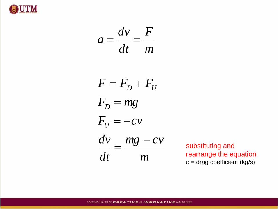
m

cvmg

dt

dv

cvF

mgF

FFF

m

F

dt

dva

U

D

UD

substituting and

rearrange the equationc = drag coefficient (kg/s)

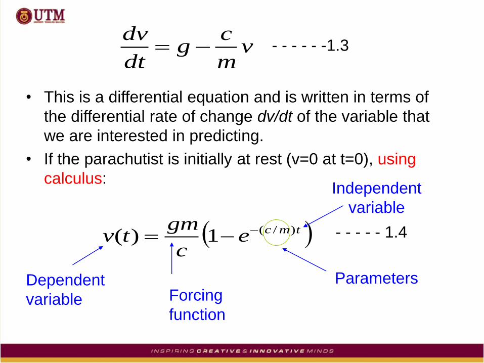
• This is a differential equation and is written in terms of

the differential rate of change dv/dt of the variable that

we are interested in predicting.

• If the parachutist is initially at rest (v=0 at t=0), using

calculus:

vm

cg

dt

dv

tmcec

gmtv )/(1)(

Independent

variable

Dependent

variable

ParametersForcing

function

- - - - - 1.4

- - - - - -1.3

Equation (1.4) is called an analytical or exact

solution because it exactly satisfies the original

differential equation.

Unfortunately, there are many mathematical models

that cannot be solved exactly.

In many cases, the only alternative is to develop a

numerical solution that approximates of the exact

solution.

As stated previously, numerical method are those in

which the mathematical problem is reformulated so it can

be solved by arithmetic/mathematics operation

Example 1.1 :

Analytical/Exact Solution of Falling Parachutist Problem

Problem statement: A parachutist of mass 68.1 kg jumps

out of a stationary hot air balloon. Use equation (1.4) to

compute velocity prior to opening the chute. Drag

coefficient (c) is equal to 12.5kg/s.

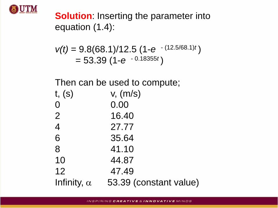
Solution: Inserting the parameter into

equation (1.4):

v(t) = 9.8(68.1)/12.5 (1-e - (12.5/68.1)t )

= 53.39 (1-e - 0.18355t )

Then can be used to compute;

t, (s) v, (m/s)

0 0.00

2 16.40

4 27.77

6 35.64

8 41.10

10 44.87

12 47.49

Infinity, 53.39 (constant value)

• Thus, according to the model (Fig. 1.2), at initial stage the

parachutist accelerates rapidly.

• Then, a velocity of 44.87 m/s is attained after 10 s.

• After sufficient time, a constant velocity, called as terminal

velocity of 53.39 m/s is reached.

• This velocity is constant because the force of gravity (FD ) is

balanced with the air resistance (FU).

• Thus, net force is zero & acceleration has ceased or stop to

increase.

Fig. 1.2 : Parachutist

accelerates rapidly

Apply Numerical methods in theNewton 2nd Law

(Falling Parachutist Problem)

• The time of change of velocity (acceleration, a ) can

be approximated by:

• Equation 1.5 is called finite divided difference

approximation of the derivative at time ti

- - - - - 1.5

dv

dtv

tv(ti1) v(ti)

ti1 ti

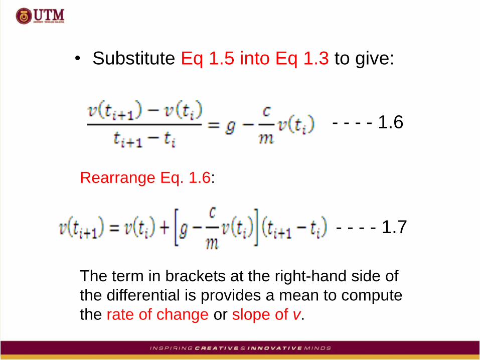
• Substitute Eq 1.5 into Eq 1.3 to give:

- - - - 1.6

- - - - 1.7

The term in brackets at the right-hand side of

the differential is provides a mean to compute

the rate of change or slope of v.

Rearrange Eq. 1.6:

Fig. 1.3 : Use of a finite difference to approximate the

first derivative of v respect to t

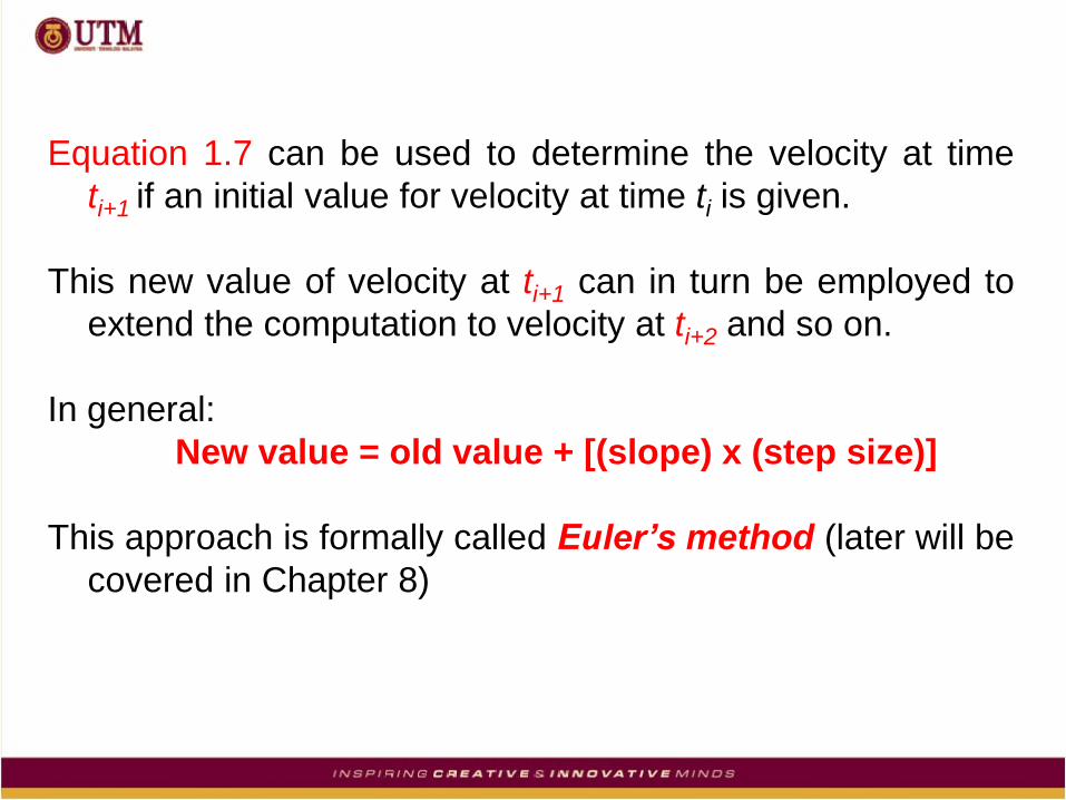
Equation 1.7 can be used to determine the velocity at time

ti+1 if an initial value for velocity at time ti is given.

This new value of velocity at ti+1 can in turn be employed to

extend the computation to velocity at ti+2 and so on.

In general:

New value = old value + [(slope) x (step size)]

This approach is formally called Euler’s method (later will be

covered in Chapter 8)

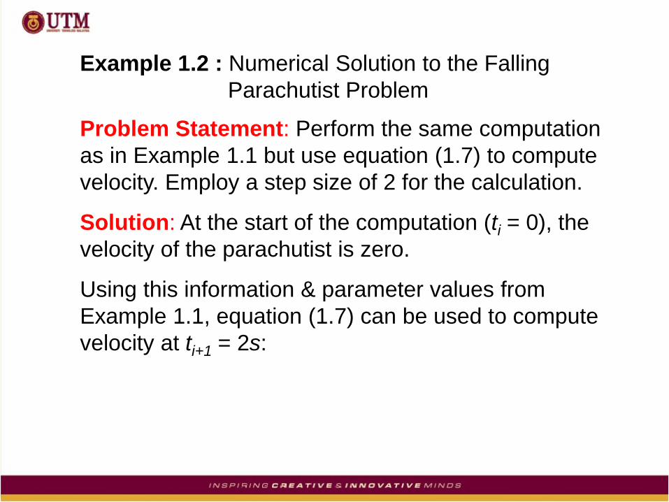
Example 1.2 : Numerical Solution to the Falling

Parachutist Problem

Problem Statement: Perform the same computation

as in Example 1.1 but use equation (1.7) to compute

velocity. Employ a step size of 2 for the calculation.

Solution: At the start of the computation (ti = 0), the

velocity of the parachutist is zero.

Using this information & parameter values from

Example 1.1, equation (1.7) can be used to compute

velocity at ti+1 = 2s:

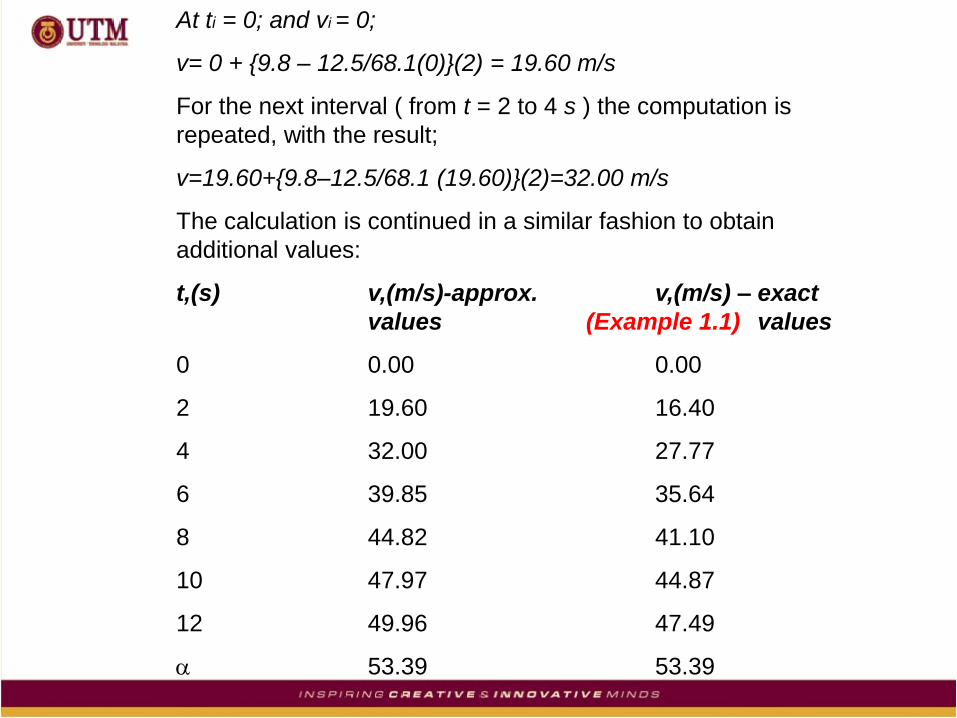
At ti = 0; and vi = 0;

v= 0 + {9.8 – 12.5/68.1(0)}(2) = 19.60 m/s

For the next interval ( from t = 2 to 4 s ) the computation is

repeated, with the result;

v=19.60+{9.8–12.5/68.1 (19.60)}(2)=32.00 m/s

The calculation is continued in a similar fashion to obtain

additional values:

t,(s) v,(m/s)-approx. v,(m/s) – exact

values (Example 1.1) values

0 0.00 0.00

2 19.60 16.40

4 32.00 27.77

6 39.85 35.64

8 44.82 41.10

10 47.97 44.87

12 49.96 47.49

53.39 53.39

Along with the exact solution, the results above are

plotted in Fig. 1.4.There are differences/discrepancy

between the two results.

One way to minimize such differences is to use a

smaller step size. With the aid of computer, large

number of calculation can be performed easily.

Thus, you can model the case without having to solve

the differential equation exactly (calculus approaches) .

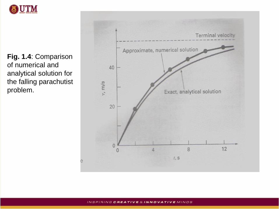
Fig. 1.4: Comparison

of numerical and

analytical solution for

the falling parachutist

problem.

Other Complicate Engineering Cases

Aside from Newton’s 2nd law, there are other major principles in

engineering.

For example the conservation laws of science & engineering:

Change = increases – decreases - - - - - 1.8

If change is zero, equation (1.8) becomes;

Change = 0 = increases – decreases

or

Increases = Decreases - - - - - 1.9

Thus, if no change occurs, the increases & decreases must be in balance,

which can be called as steady state computation – that has many

applications in engineering.

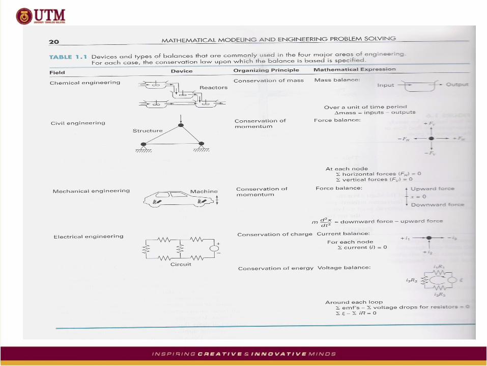
Table 1 summarizes some of simple engineering

models.

Most of chemical engineering applications will focus on

mass balance for reactor – depends on mass flow in &

out.

Both the civil & mechanical engineering applications

will focus on conservation of momentum.

Electrical engineering applications employ both

current & energy balance to model electric circuits.

For steady-state incompressible fluid flow in pipes:

Flow in = Flow out

Or

100 + 80 = 120 + Flow4

Flow4 = 60

END

OF

CHAPTER 1