CHEM 3430Analytical Chemistry II

Winter Semester, 2004© University of Guelph

Lecturer: Dr. Perry Martos, CIH

2

Course Objectives

• The overall aim of this course isto develop an understanding ofthe fundamental aspects ofanalytical chemistry used intoxicological considerations:– Target analyte extraction and

concentration– Chromatography and detectors– Mass spectrometry– Hyphenated techniques– Spectroscopic techniques– Electrochemical approaches– Data analysis

3

Topics• Data Reduction and Analysis• GLP, Terms and Definitions• Target analyte extraction and concentration

– LLE, SPE, SPME

• Chromatography and Detectors– LC, GC, CE, size exclusion, affinity– FID, NPD, PFD, PID, ECD, MS, MS/MS, MSn

• Mass spectrometry– Quad, Tandem Quad, Ion Trap, Sector

• Hyphenated techniques– LC-MS, LC-MS/MS, GC-MS, GC-MS/MS,

CE-MS and CE-MS/MS

• Spectroscopic techniques– UV/VIS, Fluorescence, AAS, AES, AFS, ICP

• Electrochemical approaches– Potentiometry and Voltammetry

4

The Analytical ProcessSample

Preparation

Extraction andConcentration

Target AnalyteSeparation

Target AnalyteDetection

Quantification

The (accuate) Result

Qualtitative orQuantitative?

Qualification

5

Qualitative and Quantitative• Ideally, determine a target analyte both

qualitatively and quantitatively.• Another way to consider: provide absolute

confidence the target analyte is present,when detected, and at what concentration(within a confidence limit).

• The use of chromatography and MS/MSand MSn permits this.

• The use of several (different) detectorseither in series or in parallel, e.g., GCcoupled PID and FID.

• Different columns with the same detector,e.g., analysis of organochlorines by GC-ECD with both a 5% phenyl column and a35% cyano column. Analytes havedifferent retention times on the differentcolumns.

6

Target Analytes• In most analyses, we require what is

called the “trace” and “ultra-trace”detection and determination of targetanalytes.– Trace has usually been defined as ppm

and sometimes ppb (ppmv in air)– Ultra-trace detection is considered at

levels of ppt and ppq

• Sometimes those analytes are“insult” environmental pollutants,pesticides, drug residues in meats,pharmaceuticals in blood…

• Methods and instruments inanalytical toxicology must be bothsensitive and selective for targetanalytes.

7

Concentrations• In water, blood,

urine, foods, soil,etc., the units oftarget analyteconcentration aretypically reportedas (wet or dry):

• ppm

• ppb

• ppt

• ppq

gµgor

mLµg

gpgor

mLpg

gngor

mLng

gfgor

mLfg

• In gases, such asair, the units ofanalyteconcentration aresometimes inmass/volume andsometimes involume/volume -be careful aboutcomparing vol/voland mass/volume

• ppmv

• ppbv

LµL

LnL

8

Airborne Concentrations• The airborne concentration of an analyte

that is either a gas or a vapour is typicallyrepresented in one of three manners: ppmv,% by volume, or mg/m3. Here is whereyou must be careful. When the unit ofconcentration is reported as mg/m3, youmust be aware of both the temperature andpressure at which this assessment wasmade. RH is also important.

• Example: an air sample using a charcoal samplingbed and a mass flow controlled air sampling pumpis taken over eight hours in a factory where styreneis used. The mass of styrene on the charcoal bed isdetermined to be 10 µg using NIOSH method3500/3501. The volume of air sampled was 50mL/min for 480 min. What is the average eighthour styrene concentration in ppmv and mg/m3 ifthe pressure and temperature during sampling were720 mm Hg and 30°C. Compare to styrene’s TLV(Ministry of Labour and NIOSH).

9

Airborne Concentrations• Consider the following for the ppmv

calculation:– Convert the mass of styrene to the volume it

would occupy at the specified averagetemperature and pressure.

• Consider the following for the mg/m3

calculation:– The use of a mass flow controlled air sampling

pump does not require additional correctionssince these pumps increase or decrease involumetric flow rate to compensate fordecreases or increases in atmospheric pressure,respectively. With automatic temperaturecorrection, the opposite is true. A conventionalair sampling pump, i.e., not mass flowcontrolled, would require correction, relative tohow it was calibrated.

• For aerosols, mass/volume is typical.– Equivalent volume diameters

10

Useful Unit Equivalents

11

Terms and Definitions• Several “Current” References on terms and

definitions for analytical methods• Need to understand GLP (Good Laboratory

Practices)• All analytical methods used for defining analyte

concentrations of significance are movingtoward GLP standards. Example: test methodsfor pharmaceuticals and pesticides

• ISO– http://www.iso.org/iso/en/ISOOnline.openerpage

• SCC– http://www.scc.ca

• Harmonized requirements IUPAC/ ISO/ AOAC– http://www.scc.ca/publicat/canp/1598_e.doc

• Overall: The analytical toxicologist has accessto terms and definitions for analytical methods

Data Analysis:Quantitative Statements about

Instrument and MethodPerformance

13

Quantitative Description ofInstrument Performance:

Why is it required?

• To (quantitatively) describe instrumentperformance so that analytical measurements ofunknowns can result in a quantitative result.

• Example: The analysis of steroids in urine; theanalysis of caffeine.

• Control charting– Monitor method performance over time. Method

performance can be distinct from instrumentperformance. Ensures the capture of “drifts” in themethod.

14

Analytical MethodConsiderations

COST

SPEED NEEDS

• COST: Training, equipment...• SPEED: When is it required...• NEEDS: e.g., a required detection limit...• Overall: An equal balance among the three is

often required.

15

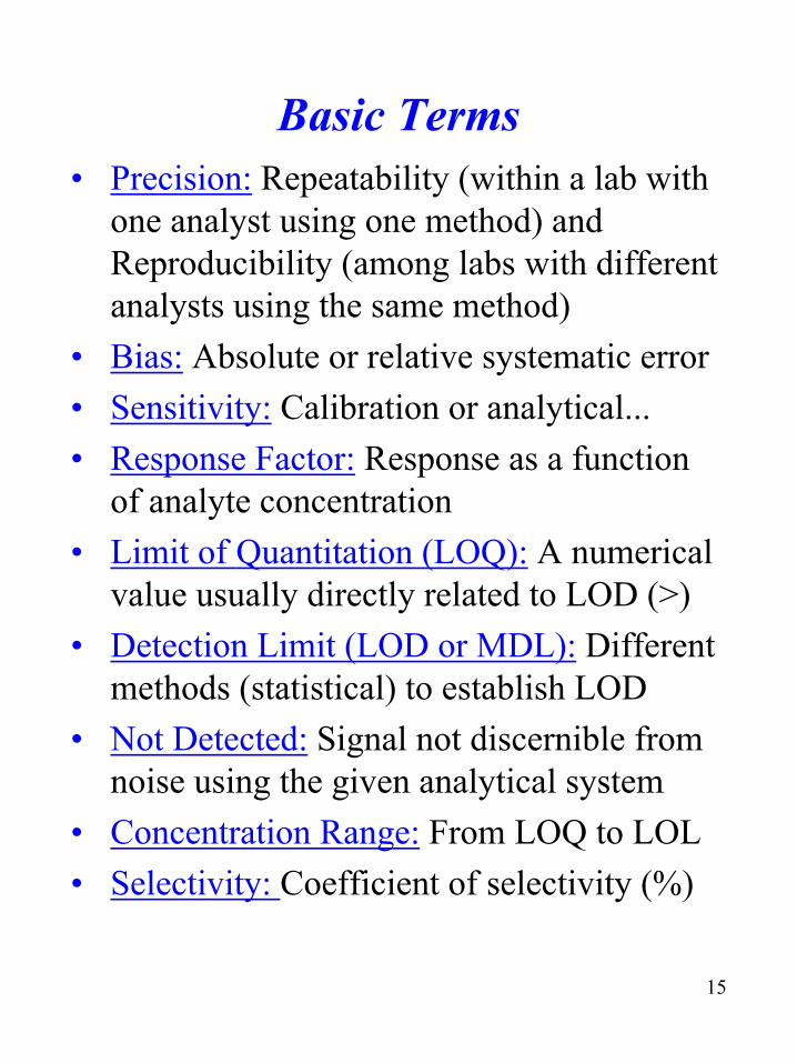
Basic Terms• Precision: Repeatability (within a lab with

one analyst using one method) andReproducibility (among labs with differentanalysts using the same method)

• Bias: Absolute or relative systematic error• Sensitivity: Calibration or analytical...• Response Factor: Response as a function

of analyte concentration• Limit of Quantitation (LOQ): A numerical

value usually directly related to LOD (>)• Detection Limit (LOD or MDL): Different

methods (statistical) to establish LOD• Not Detected: Signal not discernible from

noise using the given analytical system• Concentration Range: From LOQ to LOL• Selectivity: Coefficient of selectivity (%)

16

• Standard Deviation (s)for a small set of data.

• Rel. Standard Deviation (using arithmetic mean)

• %RSD or CV (Coefficient of variation)

• Standard Deviation of the Mean

• Variance

• Overall standard deviation - Uncertainty( ) ( ) ( ) ( )22

32

22

1 ... Nsssss +++=

2sNssm =

1

)(1

2

−

∑ −= =

N

xxs

N

ii

%100⋅= xsCV

xsRSD =

N

xN

ii∑ −

= =1

2)( µσ

Smallset ofdata

Population

Precision

17

• Variance (s1)2 of TEST METHOD #1 (sample)

• Variance (s2)2 of TEST METHOD #2 (sample)

• The ratio of variances (where S22 >S1

2)

21s

22s

21

22

SSF =

Gaussian(Normal)

Distributions

F-test: Comparison of Variances

18

• Mean of TEST METHOD #1 (sample)• Mean of TEST METHOD #2 (sample)• Are the means equal? The t-test we use is

dependent on whether the variances of the two testmethods are the same or different. Again, assumeGaussian Distributions. One-tailed t-test for equalvariances, and two-tailed for unequal variances.The two-tailed presents more relaxed constraints onestablishing equivalence.

1X

2X

t-test: Comparison of Means

19

Accuracy and Precision...

• Before we can appreciate the term Bias, we mustfirst understand the basic terms “accuracy” and“precision”.

• Accuracy is generally accepted as the closeness of a“result” to that of an expected value.

• Consider the following example:– 10 µL of each 1, 5, 20, and 100 ppm standards of

caffeine standards (USP grade) are injected into anLC-MS. An external standard calibration curve isgenerated.

– 10 µL of a “reference” (NIST traceable) samplecontaining caffeine of a concentration unknown tous, is then injected into the LC-MS. The response,once interpolated from the calibration curve, yields10.4 ± 0.2ppm (95%) in the sample.

– We find out later that the actual concentration of the“reference” caffeine standard is 10.1 ± 0.1ppm(95%).

– Is your result accurate? Why?

20

...Accuracy and Precision...

• We must appreciate that the so-called determinationof an analyte concentration in a sample is really, atbest, an “estimate” of its actual concentration.

• Associated with every determination is a level of“precision”.

• Consider the following continuing with our caffeinedetermination: (Note, the red bar is the “expected”concentration of the target analyte and is 10 ppm.)

5-

10-

15-ppm

• 10 measurements, withan averageconcentration of 10.1ppm, yet the range ofconcentrations is >20%RSD.

• Accurate Not Precise

21

...Accuracy and Precision...

5-

10-

15-ppm

• 10 measurements,with an averageconcentration of 12ppm and with>20% RSD.

• Not Accurate andNot Precise

5-

10-

15-ppm

• 10 measurements, withan averageconcentration of 12ppm, yet with <10%RSD.

• Precise Not Accurate

22

...Accuracy and Precision

5-

10-

15-ppm

• 10 measurements, with anaverage concentration of10.4 ppm, and with <2%RSD.

• PRECISE, but is itACCURATE?

• From this, we can see clues re. BIAS, t-testcomparison of means of results usingdifferent methods (ANOVA), LOD, LOQ,and even ruggedness.

Accuracy, Precision, ND, LOD, LOQ,Selectivity, Sensitivity, Linearity,Ruggedness

23

Bias and ErrorsPage 12-on and A2-A5 Skoog Holler Nieman

• BIAS: The systematic departure of the “measured”value from the “true” or “expected” value.

• There are many sources of BIAS, and they may beadditive.

• Accuracy can be assessed quite simply usingcertified or standard reference materials that“match” your test standards and samples.

– Matrix effects can create artifacts resulting in BIAS,positive or negative.

•• SYSTEMATIC ERRORS can result in BIAS.SYSTEMATIC ERRORS can result in BIAS.• A: No BIAS; B: BIAS +ve

24

Errors...

• Three basic types:– Instrumental– Method– Personal

Overall:• Systematic or determinate• Random - indeterminate• Mistakes (human errors,

or prejudice) - determinate

Instrumental Errors• “Drift” in electronic circuits (e.g., improper zero)• Temperature control is unstable is subject to

ambient parameters.• Poor power supplies, e.g., other instruments on the

same power grid perturbing the instrument’s power.• Other systems in the area creating a field that

influences detector response, coincidentally whilethe samples are running, but not the standards.

• Regular calibration is required, the frequency ofwhich is for the most part empirically determined(from actual experiments).

In all cases, accuracy is most likely affected

25

...Errors...

Method Errors• Often introduced by non-ideal chemical behavior.• Loss of sol’n by evaporation.• Analyte losses upon unexpected adsorption or

absorption.• Contaminants.• Interferences (affects selectivity, e.g.,

electrochemical methods, AA)• Instability of reagents.• Difficult to detect the target analytes.• The solution is usually to prepare the standards in

the same matrix as the samples. This can be easilyaccomplished by Standard Addition, IsotopeDilution (deuterated analogues), and InternalStandard approach (preferably with deuteratedanalogues). This is where External StandardCalibration can result in BIAS.

• Use of CRM (certified reference materials),intralaboratory method validation, and verificationby other analysts really helps here.

26

...Errors...

Human (Personal) Errors• Made unknowingly and sometimes knowingly.• Prejudice w.r.t. reading meniscus, thermometers,

pH meters, peak integration (apex determinations),colour end points.

27

...Errors...

Sources of BIAS and VARIABILITY in the Lab• Sample storage (contamination, physical or

chemical degradation)• Sample handling (contamination during

preparation).• Sub-sampling• Weighing and volumetric devices• Solvent purity• Extraction yields - low and/or variable• Analyte concentration following evaporation• Clean-up steps (analyte losses)• Quality of reference standards• Instrument calibration• Instrumental - injection variability and/or

discrimination, matrix effects, changes in detectorresponse during the course of the sample analyses

• Different analysts• Environmental and electrical conditions in the lab

(T, RH).

28

...Errors

Assessing BIAS and Variability• Use of reference materials• Comparison to another method (preferably a

standard method)• Use of representative blank matrices and spikes• Use of true positive samples and spikes, which

have been confirmed by other analysts or lab• Within-run and between-run variability studies

29

Comparison to Another Method

30

Comparison to a Reference Value

31

32

33

A Look At Calibration Curves:

• Does r² adequately indicate linearity in alinear least squares regression?

• R² is often used to describe linearity, butbe very careful, since extreme bias canbe realized at low concentrations -example to follow.

• Comment: Use Response Factors (RF)(Response/unit concentration)

• What about weighting? (1/x)• What about non-linear functions? Look

at 2nd order:( )

arespyabb

Conc2

)int(42 −−±−=

( )slope

yrespConc int−=bmxY +=

cbxaxY ++= 2

34

• Linear Least Square Regression, Unweighted• Ideal Calibration Curve• Y-Int=0

Curve 1

y = 5.00000xR2 = 1.00000

0

2000

4000

6000

8000

10000

12000

14000

16000

18000

0 500 1000 1500 2000 2500 3000 3500

[ ] ppm

Res

pons

e

ppm Arb Units1 55 2525 125

125 625625 31253125 15625

Curve 1

35

Curve 2

• Linear Least Square Regression, Unweighted• Here, Points 1, 2, and 3 are each increased by 100%• The calibration curve still looks good from the

perspective of r²

ppm Arb Units1 105 50

25 250125 625625 3125

3125 15625

Curve 2

y = 4.9872x + 34.165R2 = 0.9999

0

2000

4000

6000

8000

10000

12000

14000

16000

18000

0 500 1000 1500 2000 2500 3000 3500

[ ] ppm

Res

pons

e

36

Curve 3

• Point 6 is increased by only 10%

y = 5.5067x - 69.415R2 = 0.9997

0

2000

4000

6000

8000

10000

12000

14000

16000

18000

20000

0 500 1000 1500 2000 2500 3000 3500

[ ] ppm

Res

pons

e ppm Arb Units1 55 2525 125

125 625625 31253125 17188

Curve 3

37

Summary of Curve ComparisonsCurve 1 Curve 2 Curve 3

Arb Units Arb Units Arb Units ppm5 10 5 125 50 25 5

125 250 125 25625 625 625 1253125 3125 3125 625

15625 15625 17188 3125

Slope 5.00000 4.98720 5.50665Y-Int 0.00000 34.16524 -69.41482

R² 1.00000 0.99994 0.99967

Er% slope -0.26% 10.13%

Curve 1 Curve 2 Curve 3ppm ppm Er% Curve 1 ppm Er% Curve 2 ppm Er% Curve 3

1 1 0% -5 -585% 14 1251%5 5 0% 3 -36% 17 243%25 25 0% 43 73% 35 41%

125 125 0% 118 -5% 126 1%625 625 0% 620 -1% 580 -7%3125 3125 0% 3126 0% 3134 0%

• Interpolation of concentrations using the estimatedslopes and Y-intercepts

38

Use of Response Factors toUnderstand Curve Linearity

• Consider the following calibration curve. We havea value of 5 Units of “Bias” for all measurements.

• There is also detector saturation at the highest targetanalyte concentration, resulting in ~10% loss ofexpected response, common with LC-MS/MS andion trap MS

• Is this curve linear, and usable for quantitation atthe low concentration range?

y = 4.4932x + 74.4370R2 = 0.9995

0

2000

4000

6000

8000

10000

12000

14000

16000

0 500 1000 1500 2000 2500 3000 3500

[ ] ppm

Res

pons

e

ppm Arb Units1 105 3025 130

125 630625 31303125 14067

39

Analysis of Linear Calibration Curve DataUsing Response Factor

• U.S.EPA indicates that with an average RF <15%CV, the curve is linear, and with up to 25% CV onRF as acceptable for some methods.

• Note that the detection limit for this method willneed adjustment with the elimination of acalibration curve data point in the low end.

• It could be that this calibration curve is truly non-linear, which is quite acceptable. The onlycondition is that CV around each point must be“low”.

Following Q-testppm Arb Units RF

1 10 5 30 6.025 130 5.2125 630 5.0625 3130 5.0

3125 14067 4.5

slope 4.5 Ave. RF 5.1Y-int 94.1 Std. Dev. 0.5

R² 0.9995 CV 11%

ppm Arb Units RF1 10 105 30 6.025 130 5.2

125 630 5.0625 3130 5.03125 14067 4.5

slope 4.5 Ave. RF 6.0Y-int 74.4 Std. Dev. 2.0

R² 0.9995 CV 34%

Original Data

40

• What strategies can be employed to establish a clearunderstanding of the calibration curve?

• What about the Dixon Test to check the RF’s.Remember, a larger Confidence is actually a lessreliable result.

• The RF data provide strong clues with respect tothe detection limit (see later).

Calibration Curve Example

NXXXXQ

−−

=1

21explowest highest to fromRank

...,, 321 NXXXX

41

• Calibration curves must appropriately reflect theanalyte concentration range of interest in thesample.

• Develop the calibration curve with more evenlyspaced data points.

• Include a number of repeat calibration curve pointmeasurements for each data point.

• Develop the calibration curve over a period of time• Ensure full multi-point calibration curve data points

are developed for each set of unknown samples,with no more than about 6 samples betweenrunning the calibration curve points.

How to avoid some of the pitfallswith calibration curves

42

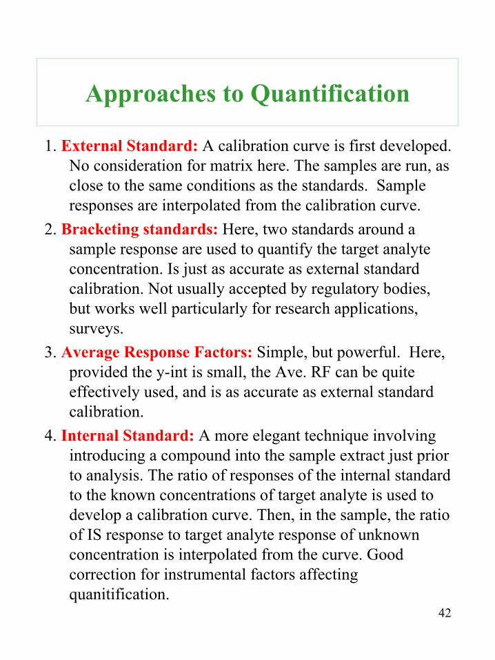
Approaches to Quantification

1. External Standard: A calibration curve is first developed.No consideration for matrix here. The samples are run, asclose to the same conditions as the standards. Sampleresponses are interpolated from the calibration curve.

2. Bracketing standards: Here, two standards around asample response are used to quantify the target analyteconcentration. Is just as accurate as external standardcalibration. Not usually accepted by regulatory bodies,but works well particularly for research applications,surveys.

3. Average Response Factors: Simple, but powerful. Here,provided the y-int is small, the Ave. RF can be quiteeffectively used, and is as accurate as external standardcalibration.

4. Internal Standard: A more elegant technique involvingintroducing a compound into the sample extract just priorto analysis. The ratio of responses of the internal standardto the known concentrations of target analyte is used todevelop a calibration curve. Then, in the sample, the ratioof IS response to target analyte response of unknownconcentration is interpolated from the curve. Goodcorrection for instrumental factors affectingquanitification.

43

Approaches to Quantification

5. Standard Addition: See Skoog Holler Nieman. Here, theactual background matrix is spiked with various (known)concentrations of the target analyte.

6. Isotope Dilution: The most elegant of all quanitificationprocedures. It involves adding an isotope of the targetanalyte to the sample prior to extraction. It therefore actsas a surrogate compound and internal standard, but mostimportantly, will elute at almost exactly the sameretention volume as the unlabelled analyte.There are various versions of isotope dilution, such asradio immunoassay and neutron activation.The ultimate isotope dilution would be to present theradioactive isotope of the target analyte to the test systemprior to incorporation into plant and animal tissue. Thiswould therefore quite thoroughly mimic the actualphysical-chemical environment of the target analyte.This strategy is actually used with new pesticideregistrations. Here, radioactive isotopes of the pesticidesare presented to plants. The fate of the pesticide can beeasily tracked.

44

Selectivity• This is a non-dimensional term, which can be

expressed in %, that can quantify the selectivity ofsystem for a specific target analyte. Let’s look atExample 1-2 in Skoog Holler Nieman (page 15).

Selectivity, Sensitivity, Signal toNoise, Detection Limit

45

Sensitivity...

• Ability of instrument to detect small changes intarget analyte concentration.

• Two factors can be used to represent sensitivity.– Slope of the calibration curve - recall this!

– Reproducibility (precision) of the measurementcan affect the sensitivity.

• Sensitivity, precision and calibrationcurves are related. The calibration curvesin the previous examples are optimal inthat s or σare negligible relative to thesignal. Also, when two calibration curveshave equal slopes, the one exhibiting betterprecision is more sensitive.

High

Low

Res

pons

e

Conc.

46

...Sensitivity

• When the confidence interval around particularmeasurements is low, we find that sensitivity iscompromised. Recall, sensitivity is the ability ofthe system to discriminate between analyteconcentrations, so “noisy” measurements results inlower confidence about sensitivity.

High

Low

Res

pons

e

Conc.

47

• IUPAC defines sensitivity as calibration sensitivity– This is the slope of the curve at the

concentration of interest. Recall ResponseFactors, where RF=Response/Conc. Note, noconsideration for precision with this approach.

Quantitative Definition of Sensitivity

blSmcS +=

Signal for“Blank”

Slope

Concentration

Signal

Res

pons

e

Conc.

48

• This definition accounts for noise at a specificconcentration. The slope can also be replaced witha response factor.

Analytical Sensitivity

sSm

=γ

StandardDeviation of

themeasurement

Slope

AnalyticalSensitivity

• Consider the use of an analytical balance. ASTMprovides guidelines on the acceptable threshold ofnoise on the sensitivity of the balance (USPreference).

• Amplification of the signal won’t be the answersince this will also increase the Ss.

• A disadvantage is that γ is concentration depend.

49

• This definition accounts for noise at a specificconcentration. The slope can also be replaced witha response factor.

Signal to Noise Ratio (S/N)(Chpt. 5, Skoog Holler Nieman)

sx

NS=

StandardDeviation of

themeasurement

MeanResponse

Signal toNoise Ratio

• This definition should look familiar...

RSDNS 1=

• What is NOISE… recall previous discussions.Simply, it is unwanted signal that can affect theproper detection and quantification of a desiredsignal. The S/N ratio has a direct impact on LOD.

50

• Noise has a direct effect on detection limit. Thedetection limit represents that concentration ofsignal which is no longer reproducibly or reliablydiscernable from noise, at which point no accuratestatement about analyte concentration can be made.Summary: we can see a signal due to the analytebut can’t exactly quantify the analyte concentration.

Noise and Detection Limit...

• Let’s review:

Not Detectable

LOD or MDL

LOQ (blank + 10 σ blank)

Estimated Analyte Concentration Using Test Method

Increasing Confidence

51

• ACS - basic definition of detection limit (seeequation below). The ACS approach is generallyaccepted; however, it has numerous limitationswhich we will explore. Note that k is usually takenas 3.

...Noise and Detection Limit...

blSblm kSS +=Standard

Deviation for“Blank”

Mean blanksignal

MinimumDistinguishable

AnalyticalSignal

mk

mSSC blSblm

m =−

=

Slope

Detection Limit

52

• Reducing noise or improving the signal will givebetter detection limits.

• For example, signal averaging (see below) appearsto pull the signal out of the noise. What ishappening here is due to the fact that “Noise isRandom”. Therefore, with enough acquired data,the noise will eventually cancel itself out. Considerthe concept of constructive and destructive waves.

• Below is an example of the effect of S/N ratio onthe NMR spectrum of progesterone.

...Noise and Detection Limit...

53

• Consider a 10 W light bulb, blue light.• In absolute darkness, that bulb, when turned on, would be

quite simple to detect. In fact, depending on the detector,say your eye, you should even be able to tell thedifference between 5 W, 10W and 15 W light bulbs.

• What if the background was contaminated, say with lightfrom one 1 W yellow light bulb.

• Now, what if the background was contaminated withlight from fifty 1 W yellow light bulbs. Would you stillbe able to see the 10 W blue light bulb with thatbackground?

The Blue Bulb...

YellowFilter

O RV

BGY

54

• It must be appreciated that detection limits are not“fixed” values, and will change with time, analyst,equipment, etc.

• Detection limits require that we can distinguishbetween a background or blank signal and a signalfrom a target analyte.

• A quantitative determination is typically taken as asystem with less than 10% RSD, less for moreserious applications such as pharmaceutical.

• The ACS has defined three important levels formeasurement of data

– LOD (blank signal+3σblank)– RDL (blank signal+6σblank)– LOQ (blank signal+10σblank)

More on S/N& Detection Limits...

55

• It must be appreciated that detection limits are not“fixed” values, and will change with time, analyst,equipment, etc.

• Normally distributed data will allow you to betterestimate the contribution of noise to your desiredsignal.

... More on S/N& Detection Limits

56

• The null hypothesis: No difference between theblank and sample (non-detect) (µA=µB).

• The alternative hypothesis: The sample response isgreater than the blank (detection) (µA>µB).

• Type I Decision Error:– Rejecting the null hypothesis when it is true (false

positive) (α)• Type II Decision Error:

– Accepting the hypothesis when it is false (falsenegative) (β)

• So, two errors are possible: False Positives andFalse Negatives depending on the hypothesis.

Type I and Type II Decision Errors

57

Decision Errors

58

Detection Limits - ACS vs. U.S.EPA

59

Detection Limits - U.S.EPA

60

S/N - Root Mean Square

61

Summary

• Significant effort is made to understand thecontribution of noise on the signal from a targetanalyte.

• Chapter 5 (Skoog) brings us into the next level ofunderstanding noise, how to manage it, and how topull out signals from what would otherwise beuseless data.

62

Analytical Instrumentation• Some critical features of an analytical

instrument:– detect the target analytes in discrete manner

(say following chromatography)– little to no background signal without sample

and/ or standard– responsive to analyte - increase in instrument

response with increasing mass loading of targetanalyte

– deliver data to the human in a discernablemanner

• Almost all instrumentation is integratedwith op amps (operational amplifiers)

• The instrument takes physicalmeasurements and converts to digital -significant advantages to working in digitaldomain

63

Instrumental Methods

64

Instruments & Components

65

Data Domains

66

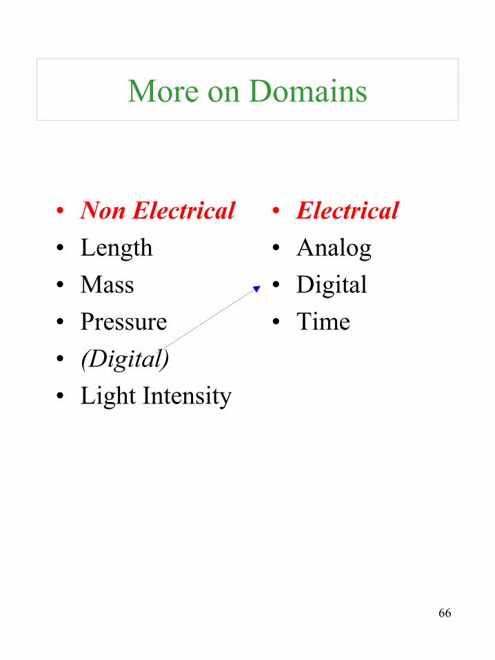
More on Domains

• Non Electrical• Length• Mass• Pressure• (Digital)• Light Intensity

• Electrical• Analog• Digital• Time

67

Interdomain Transfers

68

• Magnitude of current, voltage, charge,power

• Continuous in both amplitude and time• Analog signals are very susceptible to

electrical noise.• Noise: Signals that can interfere with the

desired signal in an analytical process.

Analog Domains

69

• Here the fluctuating signals are plotted as afunction of time….f(t), as in FTNMR,FTIR, FTMS.

• These data can be transformed tofrequency via Fourier Transformation

Time Domains

70

• Can convert Time-Domain Signals into Digital-DomainSignals

• Data are stored as a series of numbers-encoded as either 0or 1, also ON or OFF.

• Information can be stated as in Fig. 1-5 (Logic LevelSignal) Number 14 - explain.

• A better method is to encode data into Binary Numbers -stored as a bit.

Digital Domains

71

• Data are stored as a series of numbers-encoded aseither 0 or 1, also ON or OFF.

Binary Code

72

• Resistance Ohms

• Current Amps

• Voltage Volts

• Capacitance Farads

• Energy Joules

• Power Watts

• Coil (Inductance) Henry’s

Useful Electrical Terms

3

2

sAmkg⋅⋅

c)(Charge/seA

32

2

sAmkg⋅⋅

2

42

mkgsA

⋅⋅

3

2

smkg ⋅

22

22

sAmkg⋅⋅

2

2

smkg ⋅

73

Overall Noise• We can expect that individual aspects of an

analytical measurement, when combined, result inan “overall noise”, which can be generallydescribed with the equation “sum of variances”.

• e.g. G=glassware, C=Chemical, I=Instrument.• S (overall) can be minimized by ensuring the the

individual noise components are controlled:– Class A glassware– Controlled environmental conditions– Well-designed instrumentation

2222

22222

...

...

nICG

nICG

SSSSS

SSSSS

+++=

+++=

Signals & Noise,Signals & Noise,Noise FiltersNoise FiltersChapter 5, Skoog

74

Instrumental Noise

• Four primary groups of InstrumentalNOISE:– Thermal (Johnson)

– Shot

– Flicker

– Environmental

fkTRvrms ∆⋅= 4

fIeirms ∆⋅= 2

fFN

1=

75

Thermal Noise

• Generally speaking, caused by electron flow (or othercharged carriers) through components in an instrument.Basically, thermal agitation of charge carriers(electrons/holes).

– E.g. Through resistors, capacitors, electrochemicalcells.

• Thermal noise: fkTRvrms ∆⋅= 4• Boltzmann’s constant: 1.38x10-23 J K-1

• T is temperature, K• R is resistance, Ω• ∆f is Bandwidth, Hz (range of frequencies)

• Note that the equation shows that thermal noise isactually independent of the actual frequency. This noiseis sometimes referred to as “White” Noise.

• Cooling key components reduces both T and R, therebyreducing thermal noise. So, cooling from RT to 77 K(with liq N2) will halve the white noise.

• Note that narrowing bandwidths makes the instrumentsluggish.

76

Shot Noise

• Generally speaking, caused by electron flow (or othercharged carriers) through junctions in an instrument.

– Across pn junctions, across the vacuum from anodeto cathode, in photocells…later.

• Shot noise: fIeirms ∆⋅= 2• I is the average direct current, A• e is the charge on the electron, 1.60x10-19 C• ∆f is the bandwidth of frequencies being considered.

• Note that the equation shows that shot noise is actuallyindependent of the actual frequency. This noise issometimes referred to as “White” Noise.

• Reducing the bandwidth is the key to reducing this noise.• But remember that narrowing bandwidths makes the

instrument sluggish!

77

Flicker Noise

• Generally speaking, directly related to the inverse of thefrequency being studied.

• Flicker noise:f

FN1

=

• 1/f is the inverse of frequency being studied.

• The origins of flicker noise are not understood.• This noise can be reduced by using AC or modulated

signals…later.• Only really significant at f<100Hz

F lic k e r N o ise D e p e n d e n c e

0

1

2

3

4

5

6

7

8

9

1 0

0 0 .1 0 .2 0 .3 0 .4 0 .5

1 /f

Vol

tage

(V, D

.C.)

78

Environmental Noise

• The low frequency noise is “Flicker” and the rest isradiant energy, motors, mechanical vibrations, AM, FM,TV.

• The reduction of all forms of noise is important inachieving the ultimate detection limit.

• Two “quiet” regions. From ~3 Hz to 60 Hz, and fromabout 1KHz to about 500 kHz (AM frequency).

79

Ensemble Averaging

• Successive (replicate)data stored as anarray, and added.

• NMR and FTIR• Skoog Holler Nieman

p107

nNS∝

Software Techniquesto Remove Noise(To Increase S/N)

80

S/N

• Nyquist (sampling) Theorem– Data acquisition frequency must be at least 2X (usually

10X) the highest frequency of the signal– delta t is the time interval between signal samples

tf

∆=

21

nNS∝

81

Boxcar Averaging

• Assumes that noise is random, and that the signal variesslowly with time.

• Average of a small number of adjacent data points, yieldsa response this is better than 1 point. (Nyquist SamplingTheorem).

82

Shielding and Grounding

• Noise arising fromenvironmentallygeneratedelectromagnetic radiationcan be reduced byshielding and grounding.

• Electromagnetic radiationis absorbed by the shieldrather than by theenclosed conductor,particularly true when thecable is carrying smallcurrents.

• Ground everythingthrough a single point toavoid capacitivecoupling.

Hardware Techniquesto Remove Noise(To Increase S/N)

83

Difference andInstrumentation Amplifiers

• Noise rejection circuits.• Later when we learn about operational amplifiers.• Before we learn about amplifiers, we have to cover basic

RC circuits (resistance-capacitance).

84

Modulation

• Hollow cathode lamp in Atomic Absorption• Amplification of DC signals is often troublesome due to

Flicker Noise• Low frequency signals are often converted to higher

frequency signals - MODULATION

• Modulation is also used in IR spectroscopy (wavelength)modulation (FTIR).

• We will learn more about this later.

85

Signal Chopping:Chopper Amplifiers & Lock-In Amplifiers

• Somewhat similar concepts - chopper• Signal is converted to square waves (Chopper)• Can detect modulated signals by following reference ν (LIA)

– Can recover signals even when S/N<1.• Atomic Absorption is a good example (Ch. 9, Skoog)

HollowCathode

Lamp

Chopper

MirroredReference

(split)

Impingeson Sample

Sample

ModulatedSignal

HardwareandSoftware

86

Analog FiltersLow Pass Filter

Skoog Chapter 2

• Common to use Low Pass Filters.• Attenuates high frequency noise and passes low

frequency signals.• This concept is used with speakers - woofer requires low

pass filter (5 to 200 Hz) (could use a loop as well). Thetweeters require high pass filter (12 to 20 kHz).

87

Operational AmplifiersOperational Amplifiers(Op Amps)(Op Amps)

88

Characteristics & Propertiesof an Op Amp

• An OP AMP is usually made up of:– resistors, capacitors, diodes, transistors

• It is an active device, with a power supply ofusually ± 15 V

• High gain• Fast response• Large input impedance• Small output impedance• Zero output for zero input• Cheap

• Op Amp is a term describing original use of thedevice - mathematical operations.

– Voltage amplification– Current to voltage conversion– Inverting signals– Comparing signals– Pulse shaping and formation– …many more uses….

The power supply isimplied here

89

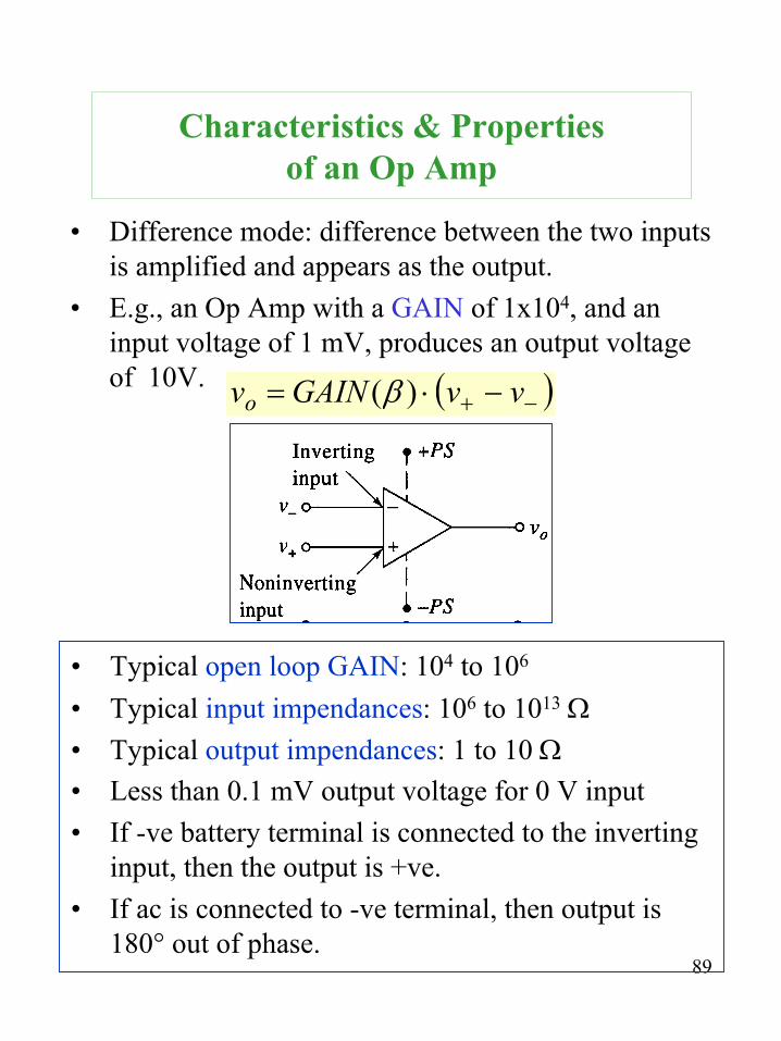
Characteristics & Propertiesof an Op Amp

• Difference mode: difference between the two inputsis amplified and appears as the output.

• E.g., an Op Amp with a GAIN of 1x104, and aninput voltage of 1 mV, produces an output voltageof 10V. ( )−+ −⋅= vvGAINvo )(β

• Typical open loop GAIN: 104 to 106

• Typical input impendances: 106 to 1013 Ω• Typical output impendances: 1 to 10 Ω• Less than 0.1 mV output voltage for 0 V input• If -ve battery terminal is connected to the inverting

input, then the output is +ve.• If ac is connected to -ve terminal, then output is

180° out of phase.

90

Limitations of OPEN LOOPOperational Amplifiers

• Even though the Gain is high (vo/vi=Gain), theprimary limitation of the “open loop” Op Amp isthe roll-off of GAIN as the signal input frequencyincreases. Limits the usefulness of the OpAmp.

• The roll-off is substantial, and is corrected byproviding “feed-back” across vo and vi

• The closed loop Gain, although lower at somefrequencies relative to the open loop, is constantover an extremely large range of frequencies.

91

CLOSED LOOPOperational Amplifiers

• This operational amplifier uses negative feedback.• It has the effect of making the Gain of the circuit

independent of the OP AMP (proof later).• Output is 180° out of phase with input.

Point S is the Summing Point.Rf is the feedback resistanceRi is the input resistanceii is the input currentif is the feedback currentiS is the current flowing into the amplifier

vi

+

-

Rf

ifRi

voiiis

S

92

• The current through Ri is given by:

• The current through Rf is given by:

• Because the input impendance of the Op Amp is so high,is is negligible (current flowing into Op Amp).

• Therefore,

• Recall that:

• So, solving for v-

• v- is negligible relative to vout and vin , and because β isso large

• Therefore,

The Inverting Op AmpSkoog Holler Nieman page 56 (sect 3B-1)

vi

+

-

Rf

ifRi

voiiis

S

( )i

ini R

vvi −−=

( )f

outf R

vvi −= −

fi ii ≅( )

f

out

i

in

Rvv

Rvv −

=− −−

)( +− −−= vvvout β

βoutvvv −= +−

0vout ≈β

f

out

i

in

Rv

Rv −

=in

out

i

f

vv

RR

−=

93

vo=

vi from v+

-ii

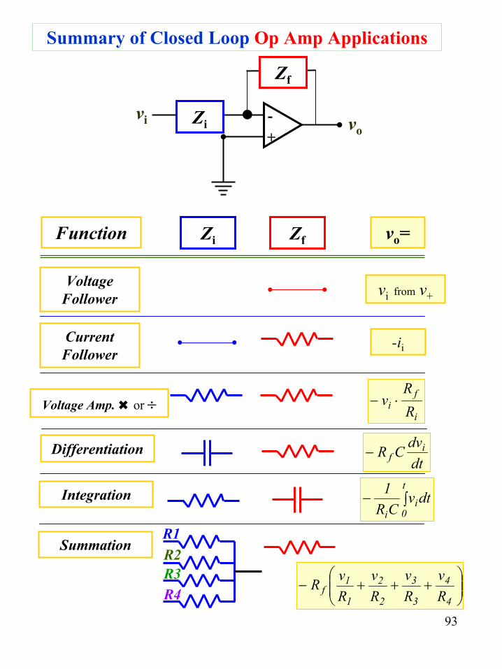
Summary of Closed Loop Op Amp Applications

vi+- vo

Zi

Zf

Zi ZfFunction

VoltageFollower

CurrentFollower

Voltage Amp. or ÷

Differentiation

Integration

Summation

dtvCR

1 t

0i

i∫−

dtdvCR i

f−

R1R2R3R4

+++−

4

4

3

3

2

2

1

1f R

vRv

Rv

RvR

i

fi R

Rv ⋅−

94

Summary of Closed Loop Op Amp Applications

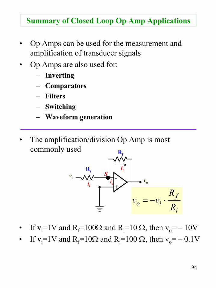
• Op Amps can be used for the measurement andamplification of transducer signals

• Op Amps are also used for:– Inverting– Comparators– Filters– Switching– Waveform generation

• The amplification/division Op Amp is mostcommonly used

vi

+

-

Rf

ifRi

voiiis

S

• If vi=1V and Rf=100Ω and Ri=10 Ω, then vo= – 10V• If vi=1V and Rf=10Ω and Ri=100 Ω, then vo= – 0.1V

i

fio R

Rvv ⋅−=

95

Voltage Follower Circuit

+

-

vivo

• This circuit is used for the accurate measurement ofpotential (voltage). Recall that we don’t want to introduce aloading error, so the Op Amp is ideal for potentialmeasurements because of its extremely large inputimpendance (~1012Ω). Application to pH measurement.

• This is a non-inverting amplifier.

−+ ≅ vv that know We oi vvvv == −+ and that and

oi vv = therefore,• This circuit has unit voltage gain, but provides extremely

large power gain related to input and output impendances.

oi vv =

RvviP

2==

o

i2

i

i

o

2o

input

output

ZZ

vZ

Zv

PP

Gain =⋅==

96

+-

Rf

if

vo

ix

Current Follower CircuitSHN p58

• Examples of current measurements include: phototubes,photomultipliers, flame ionization and electron capturedetectors (pA current outputs), voltammetry.

• These circuits provide current to voltage conversion.

fx ii ≅

fxffo RiRiv −=−=

f

ox R

vi −=∴

mL

mRR

REr+

−=%

• So, if Rf is 100 kΩ and ix is 1µA, then vo is 100 mV. Thisvoltage can be easily measured or amplified, as required.

• Loading error is important to consider with these devices...

97

Integration of Voltage Using an Op Amp

• This circuit can integrate a signal that varies as afunction of time. For example, it is used in aphotodiode array detector to integrate the magnitudeof voltage loss following direct exposure of the n-psilicon to light energy.

• There is a “reset” switch that will discharge thecapacitor, and have the circuit ready for the nextmeasurement.

vi

+

- vo

Cf

Ri

HoldSwitch

ResetSwitch

1. Open the hold switch and close the reset to discharge thecapacitor

2. Open the reset switch and close the hold switch3. Open the hold switch• This is a ramp generator

V

Time

98

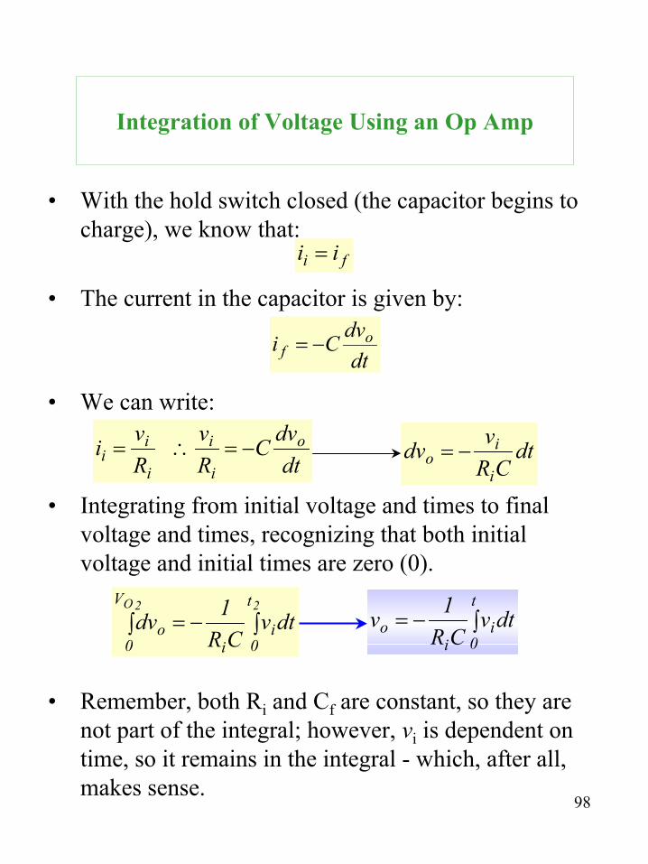
• With the hold switch closed (the capacitor begins tocharge), we know that:

• The current in the capacitor is given by:

• We can write:

• Integrating from initial voltage and times to finalvoltage and times, recognizing that both initialvoltage and initial times are zero (0).

• Remember, both Ri and Cf are constant, so they arenot part of the integral; however, vi is dependent ontime, so it remains in the integral - which, after all,makes sense.

Integration of Voltage Using an Op Amp

fi ii =

dtdvCi o

f −=

dtdvC

Rv

Rvi o

i

i

i

ii −=∴= dt

CRvdvi

io −=

dtvCR

1dv22O t

0i

i

V

0o ∫−=∫ dtv

CR1v

t

0i

io ∫−=

99

Low Pass, High Pass, and Bandpass FiltersUsing Op Amps

212c RRC2

1fπ

=

• Where fc is the low frequency cutoff.• With c), one can vary the values of R1, R2, C1, and C2

to provide integration, differentiation, and bandpassfiltering.

212c CCR2

1fπ

=1C1R2

1f1 π=

222 CR2

1fπ

=