f

, FIN,_L DRAFT 21 March 2000 SPIE Conference, Munich, Germany

Charged Particle Environment for NGST: Model Development

William C. Blackwell *a, Joseph I. Minow a, Steven W. Evans b, Donna M. Hardage c, and

Robert M. Suggs b

_Sverdrup Technology, Inc., Marshall Space Flight Center Group, Huntsville, AL 35806

bED44/Environments Group, NASA/Marshall Space Flight Center, Huntsville, AL 35812

CED03/Engineering Technology Development Office, NASA/MSFC, Huntsville, AL 35812

Abstract

NGST will operate in a halo orbit about the L2 point, 1.5 million km from the Earth, where the spacecraft will

periodically travel through the magnetotail region. There are a number of tools available to calculate the highenergy, ionizing radiation particle environment from galactic cosmic rays and from solar disturbances. However,

space environment tools are not generally available to provide assessments of charged particle environment and itsvariations in the solar wind, magnetosheath, and magnetotail at L2 distances. An engineering-level phenomenolgy

code (LRAD) was therefore developed to facilitate the definition of charged particle environments in the vicinity ofthe L2 point in support of the NGST program. LRAD contains models tied to satellite measurement data of the solar

wind and magnetotail regions. The model provides particle flux and fluence calculations necessary to predictspacecraft charging conditions and the degradation of materials used in the construction of NGST. This paperdescribes the LRAD environment models for the deep magnetotail (X6sE < -100 Re) and solar wind, and presents

predictions of the charged particle environment for NGST.

Keywords: NGST, L2, plasma, environment, magnetotail, magnetosheath, solar wind

1. Introduction

Anti-sunward of the Earth the solar wind interaction stretches the geomagnetic field for hundreds of Earth radii

forming the extended magnetotail (see Fig la). Reports of magnetotail encounters by satellites have even beenreported as far as 500 RE from the Earth, well past L2 at 236 RE. The location of the magnetopause--the outer

boundary of the magnetosphere--is determined by a pressure balance condition between the internal magnetic fieldpressure of the magnetosphere and the dynamic pressure of the magnetosheath plasma. The magnetosheath is solar

wind plasma heated upon crossing the bow shock wave formed when the supersonic solar wind flow encounters themagnetosphere. Similar to the magnetopause, the location of the bow shock (and therefore the dimensions of the

magnetosheath) is determined by the solar wind plasma interaction with the magnetosphere.

The magnetic topology of the magnetotail is supported by the neutral sheet, a current sheet flowing from dawn to

dusk across the magnetotail. Magnetic field lines in the tail are stretched in the direction of the solar wind flow, andpoint towards the Earth in the northern lobe of the magnetotail and away from the Earth in the southern lobe as

required by the direction of current flow in the neutral sheet. The relatively hot, dense plasma sheet lies at the centerof the tail and includes the neutral sheet, the central plasma sheet, and plasma sheet boundary layers. A boundary

layer forms immediately inside the magnetopause due to magnetosheath plasma that enters along open field lines.In the near Earth magnetosphere the boundary layer contains solar wind plasma that has entered the magnetosphere

through the polar cusps. As the boundary layer flows anti-sunward it also drifts toward the plasma sheet and bysome 50 Re the dominant source of plasma throughout the magnetotail is the solar wind [i]. Within 50 Re the

ionosphere provides an additional source of plasma to the lobes and plasma sheet. Between the plasma sheet andthe magnetopause are the lobes, regions of low density plasma compared to the plasma sheet and magnetosheath........................

*Correspondence: Email: bill.blackwell @msfc.nasa.g_qvl Telephone: 256 544 6741; Fax: 256 544 0242

https://ntrs.nasa.gov/search.jsp?R=20000032964 2018-07-09T13:44:13+00:00Z

f

• FINAL DRAFT 21 March 2000 SPIE Conference, Munich, Germany

rr"v

>-

-150

-100

-50

0

50

100

150100

......... I ......... i ......... * .........

Ge°sync_r_'°n°LIs BowShock

n /

.......So Wind

0 -100 -200 -300XGsE(Re)

a) b)

Bow shock

SW

Plasma

CPS

PSBL

Figure 1. Schematic of the Plasma Regimes in Earth's Magnetotail. (a) The sample halo orbit about L2 traversesall plasma regimes at L2 distances from Earth. Note the aberrated position of the magnetotail away from the Sun-Earth line due to the Earth's orbital velocity. (b) The cross section in the GSE Y-Z plane illustrates the main plasmaregimes that have been identified in the distant magnetotail (from [2]).

A cross section illustrating plasma regimes identified in the terrestrial magnetotail is given in Figure I b. Many of thedistinctions between components of individual regions (i.e., the central plasma sheet, plasma sheet, and plasma sheetboundary layer) are difficult to assign to the L2 plasma environment. However, the main magnetotail regions

identified in the near Earth magnetotail shown in Figure lb are clearly identifiable at L2 [2,3,4]. These include the

boundary layer (including the plasma mantle, lobe, low latitude boundary layer), plasma sheet (including the centralplasma sheet, boundary plasma sheet, and neutral sheet).

Halo orbits about L2 will pass through the magnetotail, magnetosheath, as well as the solar wind. Mission designs

with large amplitude halo orbits will place the satellite in the relatively high density, low energy plasma of themagnetosheath and solar wind for extended periods of time. In contrast, a mission design with a sufficiently smallamplitude halo orbit will place the spacecraft for appreciable times in the relatively low density, high energy plasma

of the magnetotail. If halo orbits with amplitudes on the order of the average diameter of the magnetotail are chosenfor the mission design, the spacecraft will encounter all of these regions during a single orbit due to the large

variability in both the size and location of the magnetotail.

In the following sections of this paper, we describe the dynamic response of the magnetopause and bow shock tovariations in the solar wind that must be considered when evaluating the plasma environment NGST will encounter

in halo orbits about L2. A brief description of the LRAD model is provided highlighting the main features of the

code and the utility for environment calculations. Examples of LRAD model output are shown including thedynamic scene generation utility, calculations of flux statistics within individual plasma regimes, and statistical orbit

fluence results for a set of hypothetical halo orbits.

2. Magnetotail Orientation and Plasma Regime Dimensions

Large scale variations in dimensions and orientation of the magnetotail and magnetosheath dimensions must beconsidered as well as the variations of plasma characteristics within individual plasma regimes when assessing the

environments a satellite may encounter in orbit about L2. The orientation and dimensions of the magnetotail and

magnetosheath at L2 distances is determined by the state of the solar wind. Since the solar wind itself is quitevariable in both density and velocity, satellites in orbit about L2 will encounter a variety of plasma conditions due to

the large scale motions of the magnetotail.

Examples of nominal and extreme variations in the bow shock and magnetotail orientations are given in Figure 2.The location of L2 is indicated to illustrate that the second Lagrange point may be located anywhere within the

t 7

FIN,_L DRAFT 21 March 2000 SPIE Conference, Munich, Germany

-2O0

-1oo

0

loo

Nominal Extreme+4 Degree Aberration +1 5 Degree Aberration

.... I .... ' .... _ .... ' ..... 200 ."' '1 ......... ' .... ' ....

-100

Ioo

-2OO

-100

0 -75 -150 -225 -300x_

Extreme-5 Degree Aberration.... I .... i .... i .... i ....

lOO

2oo75

200 .... _........... ,_,_=_ 200 .. •_..................75 o -75 -15o -225 -300 75 o -75 -I50 -225 -300

x=E x_

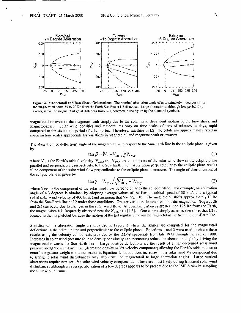
Figure 2. Magnetotail and Bow Shock Orientations. The nominal aberration angle of approximately 4 degrees shiftsthe magnetotail some 15 to 20 Re from the Earth-Sun line at L2 distances. Large aberrations, although low probabilityevents, move the magnetotail great distances from L2 (indicated in the figure by the diamond symbol).

magnetotail or even in the magnetosheath simply due to the solar wind dependent motion of the bow shock and

magnetopause. Solar wind densities and temperatures vary on time scales of tens of minutes to days, rapidcompared to the six month period of a halo orbit. Therefore, satellites in L2 halo orbits are approximately fixed in

space on time scales appropriate for variations in magnetotail and magnetosheath orientation.

The aberration (or deflection) angle of the magnetotail with respect to the Sun-Earth line in the ecliptic plane is givenby

tan fl = (Ve +Vsw,y)/Vsw,, ' (1)

where V_ is the Earth's orbital velocity. Vsw,x and Vsw,y are components of the solar wind flow in the ecliptic planeparallel and perpendicular, respectively, to the Sun-Earth line. Aberration perpendicular to the ecliptic plane resultsif the component of the solar wind flow perpendicular to the ecliptic plane is nonzero. The angle of aberration out of

the ecliptic plane is given by

itan ?' = Vsw,z w,x + Vs_,y (2)

where Vsw.z is the component of the solar wind flow perpendicular to the ecliptic plane. For example, an aberration

angle of 4.3 degrees is obtained by adopting average values of the Earth's orbital speed of 30 krrds and a typicalradial solar wind velocity of 400 km/s (and assuming that Vy=Vz = 0). The magnetotail shifts approximately 18 Refrom the Sun-Earth line at L2 under these conditions. Greater variations in orientation of the magnetotail (Figures 2b

and 2c) can occur due to changes in the solar wind flow. At downtail distances greater than 125 Re from the Earth,the magnetosheath is frequently observed near the XcsE axis [4,5]. One cannot simply assume, therefore, that L2 islocated in the magnetotail because the motion of the tail regularly moves the magnetotail far from the Sun-Earth line.

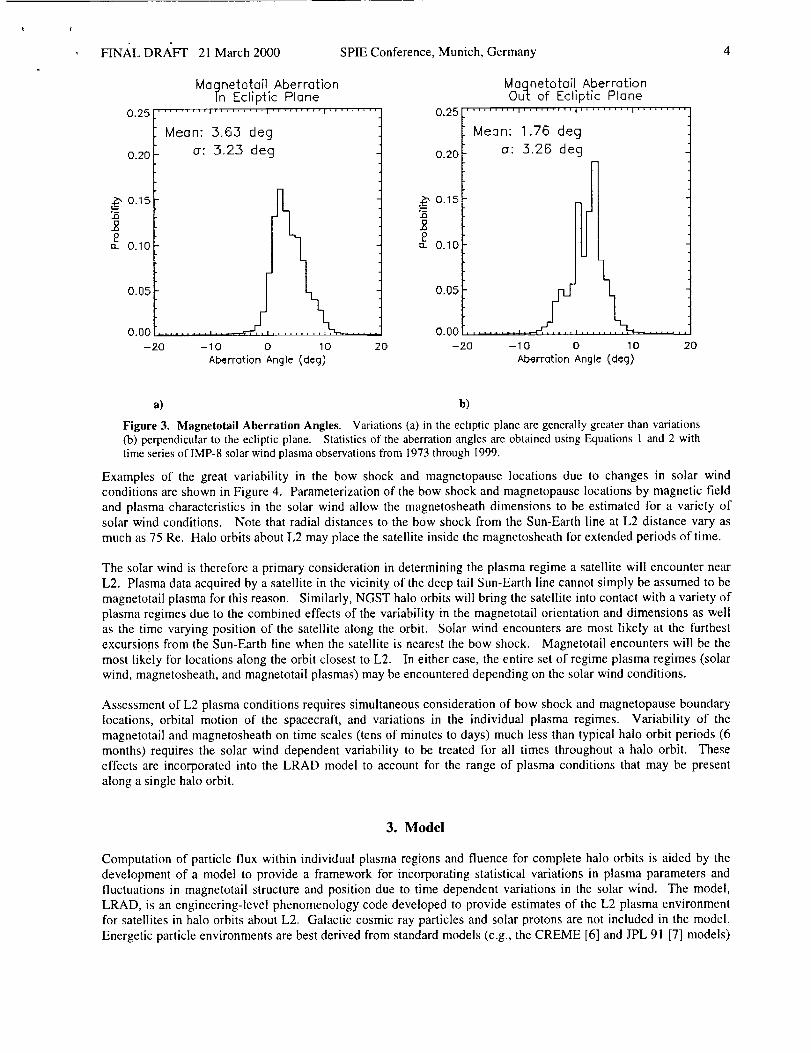
Statistics of the aberration angle are provided in Figure 3 where the angles are computed for the magnetotaildeflections in the eclipic plane and perpendicular to the ecliptic plane. Equations 1 and 2 were used to obtain these

results using the velocity components provided by the IMP-8 spacecraft from late 1973 through the end of 1999.Increases in solar wind pressure (due to density or velocity enhancements) reduce the aberration angle by driving the

magnetotail towards the Sun-Earth line. Large positive deflections are the result of either decreased solar windpressure along the Sun-Earth line (decreased density or Vx velocity component) allowing the Earth's orbit motion to

contribute greater weight to the numerator in Equation 1. In addition, increases in the solar wind Vy component dueto transient solar wind disturbances may also drive the magnetotail to large aberration angles. Large vertical

aberrations require non-zero Vz solar wind velocity components. These are most likely during transient solar wind

disturbances although an average aberration of a few degrees appears to be present due to the IMP-8 bias in samplingthe solar wind plasma.

FINP_LDR,_FF21March2000 SPIEConference,Munich,Germany

0,25

0.20

O.15:5

Pu_ 0,10

0.05

Magnetota[l AberrationIn Ecliptic Plane

...... 1,,i,, ,,,,l ,,i,, ,,,,,,,i,, .......

Mean: 3.63 deg

a: 3.23 deg

0,25

........ ! .......

-10 O 10Aberration Angle (d_g)

0.20

0.15_6

2u.. 0.10

0.05

Magnetotail AberrationOut of Ecliptic Plane

' '''' .... I ...... ' ''I'' ....... I .........

Mean: 1.76 dog

a: 3.26 deg

\-10 O 10

Aberration Angle (dog)

0.00 0.0C-20 20 -20 20

4

a) b)

Figure 3. Magnetotail Aberration Angles. Variations (a) in the ecliptic plane are generally greater than variations(b) perpendicular to the ecliptic plane. Statistics of the aberration angles are obtained using Equations 1 and 2 withtime series oflMP-8 solar wind plasma observations from 1973 through 1999.

Examples of the great variability in the bow shock and magnetopause locations due to changes in solar windconditions are shown in Figure 4. Parameterization of the bow shock and magnetopause locations by magnetic field

and plasma characteristics in the solar wind allow the magnetosheath dimensions to be estimated for a variety ofsolar wind conditions. Note that radial distances to the bow shock from the Sun-Earth line at L2 distance vary as

much as 75 Re. Halo orbits about L2 may place the satellite inside the magnetosheath for extended periods of time.

The solar wind is therefore a primary consideration in determining the plasma regime a satellite will encounter nearL2. Plasma data acquired by a satellite in the vicinity of the deep tail Sun-Earth line cannot simply be assumed to be

magnetotail plasma for this reason. Similarly, NGST halo orbits will bring the satellite into contact with a variety ofplasma regimes due to the combined effects of the variability in the magnetotail orientation and dimensions as wellas the time varying position of the satellite along the orbit. Solar wind encounters are most likely at the furthest

excursions from the Sun-Earth line when the satellite is nearest the bow shock. Magnetotail encounters will be themost likely for locations along the orbit closest to L2. In either case, the entire set of regime plasma regimes (solar

wind, magnetosheath, and magnetotail plasmas) may be encountered depending on the solar wind conditions.

Assessment of L2 plasma conditions requires simultaneous consideration of bow shock and magnetopause boundarylocations, orbital motion of the spacecraft, and variations in the individual plasma regimes. Variability of themagnetotail and magnetosheath on time scales (tens of minutes to days) much less than typical halo orbit periods (6

months) requires the solar wind dependent variability to be treated for all times throughout a halo orbit. Theseeffects are incorporated into the LRAD model to account for the range of plasma conditions that may be present

along a single halo orbit.

3. Model

Computation of particle flux within individual plasma regions and fluence for complete halo orbits is aided by thedevelopment of a model to provide a framework for incorporating statistical variations in plasma parameters andfluctuations in magnetotail structure and position due to time dependent variations in the solar wind. The model,

LRAD, is an engineering-level phenomenology code developed to provide estimates of the L2 plasma environmentfor satellites in halo orbits about L2. Galactic cosmic ray particles and solar protons are not included in the model.

Energetic particle environments are best derived from standard models (e.g., the CREME [6] and JPL 91 [7] models)

FINALDRAFT21March2000 SPIEConference,Munich,Germany

Bow Shock and Magnetopause

200_ .... J ......... _ _ ......... _ ....

__ B, (nT) V. (krn/s) Np (#lcc)

l- _l o 400 o --I- bl -s 4oo 8 ........ |

1sol- =l -is 4o0 8 ...... -" |I- d) o 7oo s ......... -'" /

'100 BS

z _" ._" .................... ..'7..'7

0 ,__,-_ _ t i c I

0 -100 -200 -300

(Ro)

Figure 4. Bow Shock and Magnetopause Variability. Case (a) and (b) are typical solar wind flows withsmall or zero Bz IMF components. Case (c) illustrates extreme locations of the bowshock for strong Bz<0conditions. Case (d) and (e) are examples of the bow shock and magnetopause response to high speed andhigh density streams, respectively. Boundary loations are derived from standard models Petrinic andRussell, [8,9] and Bennett et al., [ 10] models. Magnetotail aberration is not included here.

which can be implemented independently of the plasma model. Solar wind dependent boundaries of the

magnetosheath and magnetotail are used to provide estimates of the dimensions of individual plasma regimes at L2distances. Within each region statistics of the plasma is incorporated into the code to facilitate the computation offlux and fluence statistics.

The outer boundary of the magnetosheath in LRAD is determined by the Bennett et al., 1997 [ 10] bow shock model

which is dependent on the solar wind plasma conditions. Parameterizations of the semi-empirical Tsyganenko [11]magnetic field models are used to determine the magnetopause boundary. An alternative magnetopause model thatcould have been chosen was the Petrinic and Russell, 1993, 1996 [8,9] empirical magnetopause models. We chose

the the Tsyganenko codes since they provide a magnetic field topology in contrast to the Petrinic and Russell modelswhich provide only empirical fits to the magnetopause location (although in the current version of the code the

magnetic field structure is not in use).

Statistics for plasma regimes within the magnetotail and the magnetosheath incorporated into LRAD are obtained

from records obtained by the University of Iowa Comprehensive Plasma Instrument onboard the Geotail satellite.Plasma moments (number density, temperature, and flow velocities) from January through June 1993 were available

for analysis. Four individual orbits through the deep tail are included in the data set providing samples over a rangeof distances from 50 Re downstream of the Earth to nearly 209 Re downstream of the Earth. Although no Geotail

plasma data was available from L2 itself there is little evidence of significant variations in the number density withdistance down the magnetotail in the data examined for this document. Previous studies of the magnetotail haveshown that beyond approximately 50 Re the plasma encountered in the tail is solar wind plasma that has either

entered the magnetosphere through the dayside polar cusp or locally along the open magnetopause boundary.Therefore the plasma in the deep tail plasma composition is characteristic of the solar wind and similar temperature

characteristics are expected over a wide range of distances.

Solar wind records are not present in the Geotail data sets that provide the magnetotail plasma environment,

requiring an alternative source of solar wind records. Solar wind properties presented here are from theInterplanetary Monitoring Platform (IMP) satellites in near circular orbits with radii from 35 to 40 Re of the Earth.Solar wind statistics are obtained from data provided by the MIT Faraday Cup instrument onboard IMP-8. Data

from an interval starting in early November 1973 through the end of December 1998 are included in the study, a

period of time spanning almost three complete solar cycles

FINALDR,£FI"21March2000 SPIEConference,Munich,Germany

LRAD Organization

ILRAD E_cmive

GETFLX

PanicleFlux Slafi.s_dcs

IMCFLUEN

ParticleFlutmee Stalis'tics

IDYNSCN

DymmicScene Gex_rato r

INffInitia_a_b n

GETKALOL2 Orbit_r

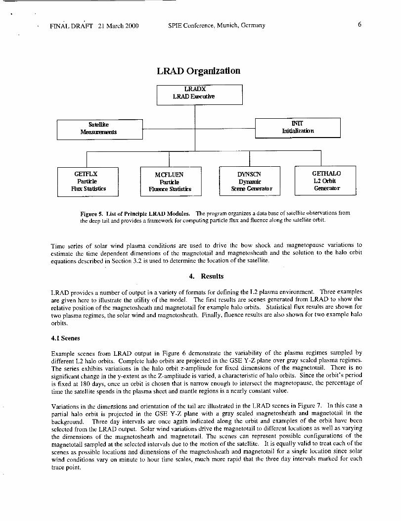
Figure 5. List of Principle LRAD Modules. The program organizes a data base of satellite observations fromthe deep tail and provides a framework for computing particle flux and fluence along the satellite orbit.

Time series of solar wind plasma conditions are used to drive the bow shock and magnetopause variations to

estimate the time dependent dimensions of the magnetotail and magnetosheath and the solution to the halo orbit

equations described in Section 3.2 is used to determine the location of the satellite.

4. Results

LRAD provides a number of output in a variety of formats for defining the L2 plasma environment. Three examplesare given here to illustrate the utility of the model. The first results are scenes generated from LRAD to show therelative position of the magnetosheath and magnetotail for example halo orbits. Statistical flux results are shown for

two plasma regimes, the solar wind and magnetosheath. Finally, fluence results are also shown for two example haloorbits.

4.1 Scenes

Example scenes from LRAD output in Figure 6 demonstrate the variability of the plasma regimes sampled bydifferent L2 halo orbits. Complete halo orbits are projected in the GSE Y-Z plane over gray scaled plasma regimes.The series exhibits variations in the halo orbit z-amplitude for fixed dimensions of the magnetotail. There is no

significant change in the y-extent as the Z-amplitude is varied, a characteristic of halo orbits. Since the orbit's periodis fixed at 180 days, once an orbit is chosen that is narrow enough to intersect the magnetopause, the percentage of

time the satellite spends in the plasma sheet and mantle regions is a nearly constant value.

Variations in the dimensions and orientation of the tail are illustrated in the LRAD scenes in Figure 7. In this case a

partial halo orbit is projected in the GSE Y-Z plane with a gray scaled magnetosheath and magnetotail in thebackground. Three day intervals are once again indicated along the orbit and examples of the orbit have beenselected from the LRAD output. Solar wind variations drive the magnetotail to different locations as well as varying

the dimensions of the magnetosheath and magnetotail. The scenes can represent possible configurations of the

magnetotail sampled at the selected intervals due to the motion of the satellite. It is equally valid to treat each of thescenes as possible locations and dimensions of the magnetosheath and magnetotail for a single location since solar

wind conditions vary on minute to hour time scales, much more rapid that the three day intervals marked for each

trace point.

FIN,_LDRAFT 21March2000 SPIEConference,Munich,Germany 7

15(3 ¸

10<3

,50

v

N _ :........__

--100

-150

150

Z-am _liLude: 125K krn Z-amplitude: 62K km15o

100

5O

0

-50

100

150

150

Z-an- Jlitude: 50K km

100 50 0 -50-100-150 150 100 50 0 -50--100-150 100 50 0 -50-100-150

YGSE (Re) YGSE (Re) YGSE (Re)

(a) (b) (c)

Figure 6. Magnetotail Cross Sections for Varying Amplitude Halo Orbits. The halo orbit amplitudes are (a) 125,000 km, (b)62,000 km, and (c) 30,000 kin. Each scene is a cross section in the GSE Y-Z plane with orbit trace points marked at 3 dayintervals. The magnetosheath is light gray, the lobes of the magnetotail dark gray, and the plasma sheet is the white strip in thecenter of the tail. The solar wind is the black background external to the light gray magnetosheath.

15(3

100

5(3

v

N--50

--103

-150

150

Z-amplitude: 125K km Z-am31itude: 125K km15Q

1O0

5O

0

-50

1O0

15O

150 100

litude: 125K km

loo 5o o -5o-loo-15o 15o lOO 5o o -5O-lOO-15o 50 o -5o-loo-15oYGSE (Re) YGSE (Re) YGSE (Re)

(a) (b) (c)

Figure 7. LRAD Scenes Illustrating Magnetotail Response to Solar Wind Variations. The orbit is the nominal 125,000 km z-amplitude case in each scene with trace points plotted at three day intervals for selected times in the orbit. Because thedimensions and position of the magnetotail and magnetosheath may vary on time scales of minutes to hours, it is possible toencounter multiple plasma regions at very short intervals of time. Shading is the same as in Figure 6.

4.2 Flux Calculations

Flux estimates are obtained from the LRAD model using a drifting Maxwellian velocity distribution in a moment

calculation. Computation of mean and limiting values of the particle flux and fluence requires a more sophisticated

analysis than that required for estimating the statistics of the individual plasma parameters. Although it is temptingto simply insert the appropriate statistical values of the plasma characteristics provided in previous sections into

equation 8, correlations between plasma density, velocity, and temperature values must be maintained since they are

FIN,_LDRP_FT21March2000 SPIEConference,Munich,Germany 8

1012

lO 10

._,-, OB

EI.-_

_g lo 6E

_E

._ lO2a

I0o

0,D01

(a)

Solar Wind Electrons: -X Flux

.-....... ,. \ Mean-

_a 95% .......

Mox

O" .....

4,

tL

.... a ....... a __LAJ_JL_ _

0.01 g.1 1 10 10D 1000

Energy (keY)

Solar Wind Protons: -X Flux1012 ........ _ ........ , ....... ._ ........ , ....... _ .......

Mean --

95% ......../_'x

"" ,"L',, _, Max- --/ / ,,,//'_x_., x, O" .....

.." /1 X_ \

..'"/.: i\',,_--" I! i\_

104 --_ _

" i,I': tl....... d ........ I ........ I ...... i[, li,iJ,l l_

0.001 0.01 0,I I 10 100 1000

(13) Energy (keV)

I(310

-_ 1o8

_ 106Eo_

O4

g0

Figure 8. Solar Wind Flux Statsties. Proton flows are dominated by the bulk motion of the plasma while theelectron flux is dominated by the thermal motion. Typical solar wind flows carry ions of a few keV in energy.Note that the mean exceeds the maximum for energies different than the peak energy due to the effect ofincluding a small number of extreme events in the averaging process.

used simultaneously to determine particle flux and fluence. A further complication arises because the fluctuatingconditions in the solar wind determine the variable dimensions of the magnetotail and magnetosheath as well as

changes in the orientation of the magnetotail. Particle flux and fluence estimates must consider this variability

because the rapid motion of the magnetosphere and magnetosheath boundaries may, for example, place the satellitewithin the magnetotail at one point in time and in the magnetosheath only a few minutes later even though the

satellite has moved only a small distance in its orbit relative to the dimensions of the magnetosphere. The combinedeffects of the orbital geometry and variability in the magnetopause and bow shock locations determine the

environment sampled by a satellite in an L2 halo orbit. Proper assessment of the environment impact on a satellite atL2 requires consideration of these combined effects.

Two important assumptions are implicit in using a drifting Maxwellian to compute particle fluxes. First, the driftingMaxwellian used in LRAD in the form [12]

\[m')3/2[ mi(v-u)2_) 2kT_f_ (r, v) = %!_ exp (3)

where the ithspecies (i = electron, hydrogen ion, helium ion, etc.) is characterized by the number density n_, mass mi,and temperature TI applies only for non-relativistic particles. This assumption is certainly valid for all plasma ionsunder consideration here since the maximum 100 keV energy considered is only a fraction of the 928 MeV proton

rest mass. Although electrons of 100 key have energies approaching twenty percent of their 511 keV rest mass,

electron energies near the peak electron fluxes are less than 1 kev for all L2 plasma regimes. Second, the originaldetermination of the number density, velocity, and temperatures from the IMP-8 and Geotail data are obtained by

implementing a numerical integration of the velocity momentsmax

<V_ >= _ v_fi(vt)AV (4)k=0

where the distribution function fi(vk) is the velocity distribution function for the ithspecies obtained by the instrument

at a discrete set of vk velocities. The observed distribution function need not necessarily be a Maxwellian to

implement this algorithm. The number density, flux, velocity, and temperature is then obtained by computing the

appropriate moment n=0,1,2 .... of the velocity distribution (c.f., Purvis et al., [12]). The original velocitydistribution functions were not available for analysis so we have assumed that all the distribution functions are

Maxwellian and compute a directional flux using the integral form

flu% = _v'fi (r, v)d3v (5)

FINAL DR_,FT 21 March 2000 SPIE Conference, Munich, Germany 9

all

w_

1o'2 ....Mean --

1010 _.'r. _-:_.-:, ,-:.. ,-, 95_ ......."..,,

"-_'_,_ _ Max - - -

_. "-. 0" .....108 , \

106 _ _'"\ \\

. "\

104 " "\ _

". "_I

! 'd10 ° _ 'l_

0.001 0.01 0.I 1 11:) 100 IOC'O

(a) Energy (keV)

1012

10 t0

_> 1o8

_ 1o6E

_q

mEu 10'*

102

100

Mognetosheoth Prot.ons: -X Flux

Mean --

95_. .......

Mc]x - -- -.

...... 2::_ :. k

" _" 'L

i i,: )

i '!1...........

0,01 0.1 1 10 100 1000

Energy (keV)

Figure 9. Magnetosheath Flux Statistics. Widths of both (a) electron and (b) ion distributions aregreater in the magnetosheath due to the conversion of bulk flow energy to thermal energy in the plasmaupon crossing the bow shock.

This assumption is not expected to create significant errors since in general the low energy plasma populations in thesolar wind, magnetosheath, and magnetotail are adequately represented by Maxwellian distributions and this

technique is reasonable for the problem at hand [13,14].

Statistics for the electron, proton, and helium fluxes are obtain using the following process: within each of theregions that plasma data is available including the solar wind, magnetosheath, plasma mantle, and plasma sheet, a

series of fluxes are computed for each data value. The correlations between density, velocity, and temperature aremaintained by using the moments in equation 3 to compute the flux with equation 4 or 5. A differential flux

spectrum is computed for each record in the data files and the resulting flux binned according to energy. Finally,the statistics of the flux within an individual energy bin is computed. The final plots and tables provided for flux are -therefore statistical flux values within individual energy ranges and should not be confused with energy spectra

Statistical results are obtained for fluxes in the solar wind, magnetosheath, plasma mantle, and plasma sheet. Lobe

and plasma mantle environments are combined into a single "plasma mantle/lobe" region in the LRAD model sincevery few lobe records were identified in the Geotail data at distances beyond -100 Re. The energy bins selectedrange from ! eV to 100 keV providing adequate coverage to those interested in material surface and thin film effects

as well as spacecraft surfacing charging analysis.

The bulk flow of the solar wind is evident in Figure 8 as the peak in the statistical proton flux for energies ofapproximately I keV, consistent with an average solar wind velocity on the order of 400-500 km/sec. Thermal

motions in the ion population is evident as the width of the the flux peaks. In contrast, the bulk flow speed of thesolar wind provides electrons with energies of only a fraction of an electron volt. Electrons are dominated bythermal motions and no obvious peak is present in the statistical fluxes.

Magnetosheath statistical fluxes are shown in Figure 9. Conversion of the bulk flow energy into thermal motion of

the plasma is evident in the ion fluxes by the enhanced fluxes at energies less than a few keV. Under averageconditions, the value of the solar wind proton flux is approximately 10s to 10 9 protons/cm2-sec-keV at energies near

1 keV. This value is reduced by a factor of 10 in the magnetosheath at 1 keV. Note however that for energies of

0.1 keV, one tenth the bulk flow energy, proton fluxes are enhanced by over three orders of magnitude. Thereappears to be two populations of electrons in the magnetosheath statistical flux plot. However, this is likely due to

undersampling the deep tail plasma populations.

4.3 Fluence Calculations

A characteristic of L2 halo orbits is that their periods are always close to 180 days, regardless of the orbit amplitude.

FINAL DRAFI" 21 March 2000 SPIE Conference, Munich, Germany 10

oto,,-,

u..._C:q.,Cq

chi

O

1020

1018

1016

10 TM

1012

1010

108

106

0.001

(o)

Z=125K krn Electrons: -X Fluence........ i ........ i ....... '1 ........ i ....... I ........

Mean --95% .......

_.,>. Max .... .• a .....

' \.,,N

":.-,,,N; X

%,\, _

", _1

0.01 0.1 1 10 t00 101)0Energy (keV)

1020

1018

_ lo16

Z=125K km ProLons: -X Fluence........ i ........ I ........ i ........ I ........ i ........

Mean --95% .......Max - - -

L'" "._.

_,_. lO 14 _ _ ..v.-' ".,,.

_ ..... .._,,_lO k

too(\ \

1°81 ,'',, '\_

1 t- ....... , ........ _ ........ i ..... \,

0.001 0.01 0.1 1Energy (keV)(b)

10 lOO 1000

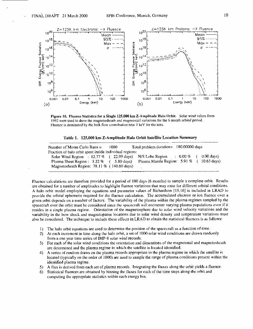
Figure 10. Fluence Statistics for a Single 125,000 km Z-Amplitude Halo Orbit. Solar wind values from

1992 were used to drive the magnetosheath and magnetotail variations for the 6 month orbital period.Fluence is dominated by the bulk flow contribution near 1 keV for the ions.

Table 1. 125,000 km Z-Amplitude Halo Orbit Satellite Location Summary............................................................................................................................

Number of Monte Carlo Runs = 1000 Total problem duration= 180.00000 days

Fraction of halo orbit spent inside individual regions:

Solar Wind Region : 12.77 % ( 22.99 days) N/S Lobe Region : 0.00 % ( 0.00days)

Plasma Sheet Region " 3.22 % ( 5.80 days) Plasma Mantle Region: 5.91% ( 10.63 days)

Magnetosheath Region: 78.11% ( 140.60 days).......................................................................................................

Fluence calculations are therefore provided for a period of 180 days (6 months) to sample a complete orbit. Results

are obtained for a number of amplitudes to highlight fluence variations that may exist for different orbital conditions.

A halo orbit model employing the equations and parameter values of Richardson [15,16] is included in LRAD to

provide the orbital ephemeris required for the fluence calculation. The accumulated electron or ion fluence over a

given orbit depends on a number of factors. The variability of the plasma within the plasma regimes sampled by the

spacecraft over the orbit must be considered since the spacecraft will encounter varying plasma populations even if it

resides in a single plasma regime. Orientation of the magnetosphere due to solar wind velocity variations and the

variability in the bow shock and magnetopause locations due to solar wind density and temperature variations must

also be considered. The technique to include these effects in LRAD to obtain the statistical fluences is as follows:

i) The halo orbit equations are used to determine the position of the spacecraft as a function of time.

2) At each increment in time along the halo orbit, a set of 1000 solar wind conditions are drawn randomly

from a one year time series of IMP-8 solar wind records.

3) For each of the solar wind conditions the orientation and dimensions of the magnetotail and magnetosheath

are determined and the plasma regime in which the satellite is located identified.

4) A series of random draws on the plasma records appropriate to the plasma regime in which the satellite is

located (typically on the order of 1000) are used to sample the range of plasma conditions present within the

identified plasma regime.

5) A flux is derived from each set of plasma records. Integrating the fluxes along the orbit yields a fluence.

6) Statistical fluences are obtained by binning the fluxes for each of the time steps along the orbit and

computing the appropriate statistics within each energy bin.

FIN,_L DR,_F'F 21 March 2000 SPIE Conference, Munich, Germany 11

1020

1018 I

1012V%,--

._,>_ 10 TM

___1012

o¢,'---"101

lO8r-i

106

O.OO 1

(o)

Z= 3OK km Electrons: -X Fluence

....... ' ........ ' ....... " ' ' 'Meon'95% ....... -

_, Max"" .'_ o- .....

". \ \

'. \ \

', _

", _,_

: %

0,01 0,1 1 10 100 1000

Energy {keY)

102o

lO 18

1016o

_ lO TMc

_1010Ld

108o

Z= 50K km Protons: -X Fluence

........ ' .....' .....' .....' Meon '9:_5%....... :Max - - -

,-.,:_ a .....,t,," -\

._.--.,'7-- --"-":"" _'" "'_\

'2",. \

106 _.,L ....... , , , ;.._.._ ......

O,OO1 O,01 0,1 1 10 100 1000

(b_ Energy {keY)

Figure 11. Fluence Statistics for a Single 30,000 km Z-Amplitude Halo Orbit. Solar windvalues from 1992 were used to drive the magnetosheath and magnetotail variations for the 6 monthorbital period. Although differing in amplitude in the z direction, the integrated flux over theperiod of one orbit is essentially the same as the case in Figure l0.

Table 2 30,000 km Z-Amplitude Halo Orbit Satellite Location Summary..........................................................................................................................

Number of Monte Carlo Runs = 1000 Total duration of problem = 180.0000 days

Fraction of halo orbit spent inside individual regions:

Solar Wind Region : 12.51% ( 22.52 days) N/S Lobe Region : 0.00 % ( 0.00 days)Plasma Sheet Region : 4.81% (8.65days) Plasma Mantle Region : 9.39% (16.89days)

Magnetosheath Region : 73.30 %............... _................................................................................... - .......................

Only representative examples are provided here for directional differential proton and electron fluences along thedirection of maximum flux, -Xgse in all cases. Complete sets of plots for the statistical differential and integrated

fluence within energy bins for each direction are produced by LRAD in the normal output.

Statistical fluences illustrated in Figure 9 are derived for the 125,000 km z-amplitude halo orbit shown in Figure 1.Solar wind data from 1992 was used to obtain the magnetopause and bow shock variations, yielding results

appropriate for solar maximum conditions. Ion fluences are dominated by the bulk flow as shown by the peak inthe fluences at energies near the peak fluxes. For comparison, Figure 10 provides a similar set of fluences for the30,000 km z-amplitude halo orbit. There is relatively little difference between the results for the large amplitude

orbit and the small amplitude orbit. Although there is a difference of 95,000 km between the z-amplitude of the twoorbits, the magnitude of the difference is less than the diameter of the magnetotail. In both cases the rate at which

the satellite will sample the magnetosheath as well as the magnetotail primarily depends on the solar wind variationsand not the orbit parameters. A summary of the statistics of the fluence calculation are given in Table 4.9 showing

the percentage of time the satellite spent in each plasma regime during the single orbit. Comparison of the orbitsummary in Table 2 with that in Table 1 indicates that the 30,000 km z-amplitude orbit samples nearly the same

plasma regimes as the 125,000 km z-amplitude orbit. The similarity is due to the fact that the solar wind drivenvariability of the magnetosheath and magnetotail is primarily responsible for moving the different plasma regimesover the satellite in the course of the halo orbit.

5. Summary

We have developed a model to aid in computing plasma environments for the L2 halo orbit proposed for NGST. Thesolar wind driven dynamics of the magnetopause and bow shock were shown to be a significant factor in determining

the plasma variability at L2. The LRAD model provides the necessary framework for computing the charged

particle flux and fluence values required to assess the plasma impacts on the NGST spacecraft. In addition, the scene

FINALDRAFT 21March2000 SPIEConference,Munich,Germany 12

generationcapabilityofLRADwasdemonstrated.Thisfunctionofthecodeisparticularlyusefulforexaminingthespacecrafttrajectoryrelativetodeeptailplasmaregimes.Finally,wenotethatthesolarwindcomponentsofLRADareequallyapplicabletotheLI environmentsothatLRADwill beusefulin theeventanalternativeorbittotheL2haloorbitischosenforthemission.

Acknowledgements

Comprehensive Plasma Instrument data from the Geotail spacecraft was generously provided by Dr. Louis A.Frankand Dr. William R. Paterson, University of Iowa. The Geotail EPIC Science Team provided the plasma regime

identifications used to classify the University of Iowa records. IMP-8 solar wind plasma records from the MITinstrument were obtained from the NSSDC data archives. Dr. Alan J. Lazarus and Dr. Karolen Paularenus, MIT, are

the Principle Investigators. We also wish to acknowledge the support of Janet Barth, Gordon Banks, and Christina

Gorsky of NASA/GSFC for obtaining a number of the data sets (courtesy of the National Space Science DataCenter). This work was supported in part by NASA Contract NAS8-80436 to Sverdrup Technology, Inc.

References

1 . Baker, D.N., and T.I. Pulkinnen, Large-scale structure of the magnetosphere,, in New Perspectives onthe Earth's Magnetotail, AGU Monograph 105, (ed. by A. Nishida, D.N. Baker, and S.W.H. Cowley),

American Geophysical Union, Washington, D.C., pp. 21 - 31, 1998.Eastman, T.E., Christon, S.P., T. Doke, L.A. Frank, G. Gioeckler, H. Kojima, S. Kokubun, A.T.Y. Lui,

H. Matsumoto, R.W. McEntire, T. Mukai, S.R. Nylund, W.R. Paterson, E.C. Roelof, Y. Saito,T. Sotirelis, K. Tsuruda, D.J. Williams, and T. Yamamoto, Magnetospheric plasma regimes identified

using Geotail meausrements 2. Regime identification and distant tail variability, J. Geophys. Res.,103, 23521 - 23542, 1998.

Bame, S.J., R.C. Anderson, J.R. Ashbridge, D.N. Baker, W.C. Feldman, J.T. Gosling, E.W. Hones, Jr.,D.J. McComas, and R.D. Zwickl, Plasma regimes in the deep geomagnetic tail: ISEE 3, Geophys. Res. Lett.,10, 912 - 915, 1983.

Christon, S.P., T.E. Eastman, T. Doke, L.A. Frank, G. Gloeckler, H. Kojima, S. Kokubun, A.T.Y. Lui,H. Matsumoto, R.W. McEntire, T. Mukai, S.R. Nylund, W.R. Paterson, E.C. Roelof, Y. Saito,

T. Sotirelis, K. Tsuruda, D.J. Williams, and T. Yamamoto, Magnetospheric plasma regimes identifiedusing Geotail meausrements 2. Statistics, spatial distribution, and geomagnetic dependence,

Fairfield, D.H., On the structure of the distant magnetotail: ISEE-3, J. Geophys. Res., 97, 1403-1410,1992.

A.J. Tylka, J.H. Adams, Jr., P.R. Boberg, B. Brownstein, W.F. Dietrich, E.O. Flueckiger, E.L. Petersen,M.A. Shea, D.F. Smart, and E.C. Smith, CREME96: A Revision of the Cosmic Ray Effects on Micro-Electronics Code, IEEE Transactions on Nuclear Science, 44, 2150-2160, 1997

J. Feynman, G. Spitale, J. Wang, and S. Gabriel "Interplanetary Proton Fluence of Model: JPL 1991,

J. Geophys. Res., 98 13281-13294 (1993)Petrinec, S.M. and C.T. Russell, An empirical model of the size and shape of the near-Earth

magnetopause, Geophys. Res. Lett., 20, 2695 - 2698, 1993.Petrinec, S.M. and C.T. Russell, Factors controlling the shape and size of the post-terminator

magnetopause, Advances in Space Research, 18, (8)2 ! 3-(8)216,1996.Bennett, L., M. G. Kivelson, K. K. Khurana, L. A. Frank, and W. R. Paterson, A model of the Earth's distant

bow shock, J. Geophys. Res., 102, 26927 - 26941, 1997.Tsyganenko, N.A., A magnetospheric magnetic field model with a warped tail current sheet, Planet.

Space Sci., 37, 5 - 20, 1989.12. Purvis, Carolyn K., Design Guidelines for Assessing and Controlling Spacecraft Charging Effects,

NASA Technical Paper 2361, 1984.13. Frank, L.A., and W.R. Paterson, Survey of electron and ion bulk flows in the distant magnetotail

with the Geotail spacecraft, Geophys. Res. Lett., 21, 2963 - 2966, 1994.

14. Paterson, W.R., and L. A. Frank, Survey of plasma parameters in the deep geomagnetic tail:

Properties of plasmoids and the postplasmoid plasma sheet, J. Geophys. Res., 90, 8872 - 8876, 1984.15. Richardson, David L., Analytic Construction of Periodic Orbits about the Collinear Points, Celestial

Mechanics 22 (1980), pp. 241 - 253.16 Farquhar, Robert W., The Control and Use of Libration-Point Satellites, NASA TR R-346, 1970.

.

.

4.

5.

6.

7.

8.

9.

10.

11.