Charged line segments and ellipsoidal equipotentials

T L Curtright§, N M Aden, X Chen, M J Haddad, S Karayev, D B Khadka, and J LiDepartment of Physics, University of Miami

Coral Gables, FL 33124-8046, USA§curtright@miami.edu

January 18, 2016

Abstract

This is a survey of the electrostatic potentials produced by charged straight-line segments, in variousnumbers of spatial dimensions, with comparisons between uniformly charged segments and those hav-ing non-uniform linear charge distributions that give rise to ellipsoidal equipotentials surrounding thesegments. A uniform linear distribution of charge is compatible with ellipsoidal equipotentials only forthree dimensions. In higher dimensions, the linear charge density giving rise to ellipsoidal equipotentialsis counter-intuitive — the charge distribution has a maximum at the center of the segment and vanishesat the ends of the segment. Only in two dimensions is the continuous charge distribution intuitive — forthat one case of ellipsoidal equipotentials, the charge is peaked at the ends of the segment and minimizedat the center.

Contents

1 Introduction 1

2 Electrostatics in two dimensions 2

3 Point charge in D dimensions 13

4 Uniformly charged line segments for all dimensions D > 2 14

5 Ellipsoidal equipotentials for all dimensions D > 2 19

6 Generalizations 25

7 Summary 26

1 Introduction

It has become a widespread practice to study the physics of systems in various numbers of spatial dimensions,not necessarily D = 3. For instance, graphene with D = 2, and string or membrane theory with D as highas 25, are two examples that immediately come to mind for both their experimental and theoretical interest.Moreover, geometric ideas provide a common framework used to pursue such studies. A pedagogical goalof this paper is to encourage students to think along these lines in the context of a familiar subject —electrostatics.

1

arX

iv:1

601.

0404

7v1

[ph

ysic

s.cl

ass-

ph]

15

Jan

2016

For example, in three spatial dimensions a uniformly charged straight-line segment gives rise to an electricpotential Φ whose equipotential surfaces are prolate ellipsoids of revolution about the segment, with the endsof the segment providing the foci of the ellipsoid. As an immediate consequence of the geometry for these

prolate ellipsoidal equipotentials, the associated electric field−→E = −

−→∇Φ — always normal to surfaces of

constant Φ — has at any observation point a direction that bisects the angle formed by the pair of linesfrom the observation point to each of the two foci of the ellipsoid. This beautiful electrostatic example waspresented by George Green in 1828 [1], and it has been discussed in many books since then [2]-[10] includingat least two texts from this century [11]. While the straight-line segment is an idealization, neverthelessit provides insight into the behavior of real thin-wire conductors, especially upon approximating those realwires as very narrow, “needle-like” ellipsoids.

But as it turns out, the line segment problem in three dimensions is a very special case, in some sense themost ideal of all possible electrostatic worlds. In any other dimension of space, uniformly charged segmentsdo not produce ellipsoidal equipotentials. Conversely, in any other dimension, if the equipotentials areellipsoidal about a linearly distributed straight-line segment of charge, then that charge distribution can notbe uniform.

One need look no farther than two dimensional systems to see clearly that there are differences betweenuniformly charged segments and those with charge distributed so as to produce ellipsoidal equipotentials.Indeed, D = 2 is the only ellipsoidal equipotential case which is intuitive in the sense that the associatedlinear charge distribution has maxima at the ends of the segment, as one might naively expect from therepulsive force between like charges placed on a segment of a real, thin conductor at a finite potential. Incontrast, the distribution of charge needed to produce ellipsoidal equipotentials is counter-intuitive in higherdimensions. To produce such equipotentials for D > 3 the charge distribution must have a maximum at thecenter and vanish at the ends of the segment.

We begin our discussion in Section 2 in two dimensions, where the two types of charged segments arereadily analyzed. Then we compare and contrast uniformly charged line segments with those admittingellipsoidal equipotentials for any number of spatial dimensions. As a preliminary, we first discuss briefly inSection 3 the potential of a point charge in D dimensions. We then use this information in Section 4 tocompute the potentials and electric fields for uniformly charged line segments. We continue in Section 5 byconsidering systems with ellipsoidal equipotentials in D dimensions. We then determine the linear chargedistributions that produce such potential configurations, and we find the remarkable result that the linearcharge density giving rise to ellipsoidal equipotentials is peaked at the center of the segment, for D > 3.

The discussion of general D affords the opportunity to illustrate how continuous D can be used as amathematical device to regulate singular behavior. This too is a widespread practice in theoretical physics.We use D in this way in Section 5 of the paper to interpolate continuously between intuitive and counter-intuitive charge distributions for segments with ellipsoidal equipotentials.

Finally, in Section 6, we invoke well-known methods to indicate how the various line segment results alsogive solutions to a class of electrostatic boundary value problems where the charge is moved outward anddistributed on one of the equipotential surfaces that surrounds the original segment.

2 Electrostatics in two dimensions

The point-particle electric potential in 2D is well-known to be logarithmic. For a point charge Q located atthe origin, up to a constant R that sets the distance scale,

Φpoint (−→r ) = kQ ln (R/r) , ∇2Φpoint (−→r ) = −2πkQ δ2 (−→r ) , (1)

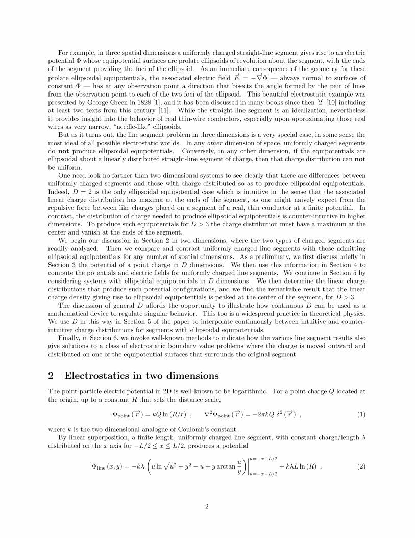
where k is the two dimensional analogue of Coulomb’s constant.By linear superposition, a finite length, uniformly charged line segment, with constant charge/length λ

distributed on the x axis for −L/2 ≤ x ≤ L/2, produces a potential

Φline (x, y) = −kλ(u ln

√u2 + y2 − u+ y arctan

u

y

)∣∣∣∣u=−x+L/2

u=−x−L/2+ kλL ln (R) . (2)

2

This result may be established by integrating the contributions of infinitesimal point-like bits of charge thatmake up the segment, using (1) and the indefinite integral∫

ln(√

u2 + y2)du = u ln

(√u2 + y2

)− u+ y arctan

u

y. (3)

Written out in full,

Φline (x, y) = kλ

(L+ y arctan

(x− 1

2L

y

)− y arctan

(x+ 1

2L

y

))(4)

+

(x− 1

2L

)kλ ln

1

R

√(x− 1

2L

)2

+ y2

− (x+1

2L

)kλ ln

1

R

√(x+

1

2L

)2

+ y2

.

A plot of the potential surface shows the essential features.

x y

Figure 1: Potential surface for a uniformly charged line segment in 2D.

The top of the potential surface is curved and not a straight line, indicating that the charged segmentitself is not an equipotential. This follows analytically from (4). Although points on the segment are notat the same potential, they are all at finite values of the potential, for D = 2. Explicitly, for y = 0 and allx,

Φline (x, 0) = kλL− kλ(

12L+ x

)ln(∣∣ 1

2L+ x∣∣ /R)− kλ ( 1

2L− x)

ln(∣∣ 1

2L− x∣∣ /R) . (5)

We plot f (x) = Φline (x, 0) /kλ versus x to show the shape of the potential along the x-axis, for L = 2 andR = 1.

3

­4 ­2 2 4

­2

2

x

f

Figure 2: Uniformly charged line segment potential for D = 2, along the x-axis.

On the other hand, transverse to the x-axis the potential has a discontinuous slope across the line segment.That is to say, the electric field normal to the line segment, Ey, is discontinuous due to the presence of thecharge density on the segment. For example, for x = 0 this transverse profile is given by

Φ (0, y) = kλ

[L− L ln

(√14L

2 + y2/R

)− 2y arctan

(12L/y

)]. (6)

We also plot g (y) = Φline (0, y) /kλ versus y to show the shape of the potential along the y-axis, for L = 2and R = 1.

­4 ­2 2 4

­2

2

y

g

Figure 3: Uniformly charged line segment potential for D = 2, along the y-axis.

Moreover, the equipotentials are not ellipses surrounding the segment on the xy-plane, as is especiallyclear for points close to the segment. The potential contours actually intersect the segment. A view of thepotential contours from below the potential surface shows these features graphically. (See the plot to follow.But note the view in that plot is actually an orthogonal projection of the contours onto the xy-plane, andnot the true perspective of an observer on the potential axis a finite distance below that plane.)

4

x

y

­2 ­1 0 1 2

Figure 4: Potential contours for a uniformly charged line segment in 2D.

The components of the electric field produced by the segment are given by

Ex (x, y) = − ∂

∂xΦline (x, y) = kλ ln

√√√√(x+ 1

2L)2

+ y2(x− 1

2L)2

+ y2

, (7)

Ey (x, y) = − ∂

∂yΦline (x, y) = kλ arctan

(L+ 2x

2y

)+ kλ arctan

(L− 2x

2y

), (8)

where we have used ddu arctanu = 1

u2+1 . Note that−→E (x, y) is independent of the scale R, since changing

R just amounts to adding a constant to the potential. But of course−→E (x, y) does depend on L as this sets

the physical length scale for the system.

As a check, in the units we have chosen the charge density along the line follows from∫ −→∇ ·−→E dxdy =

2πk∫ρ dxdy, integrated over a horizontal rectangle containing an infinitesimal portion of the x-axis, as the

height of the rectangle is taken to zero. Thus, using limz→±∞

arctan z = ±π/2,

2πk λ (x) = 2 limy→0

Ey (x, y) = 2kλ×

0 if x > L/2π if − L/2 < x < L/20 if x < −L/2

. (9)

That is to say, the charge/length between −L/2 and L/2 is the constant λ, as expected. Elsewhere, thecharge density vanishes, as follows from ∇2Φline (−→r ) = 0 for all points not coincident with the segment.

It is instructive to make a vector field plot of (Ex (x, y) , Ey (x, y)), especially near the charged segment.Again it is evident graphically that the segment itself is not an equipotential, since the electric field linesare not perpendicular to the segment as the x-axis is approached for −L/2 < x < L/2, except at the singlepoint x = 0. Here are vector field plots for L = 2.

5

­2 ­1 1 2

­2

­1

1

2

x

y

­1.2 ­1.0 ­0.8 ­0.6 ­0.4 ­0.2 0.2 0.4 0.6 0.8 1.0 1.2­0.1

0.1

x

y

Figures 5 & 6: Vector field plots of−→E for a uniformly charged line segment situated between x = −1 and

x = +1. The field is evaluated at the center of each arrow.

6

In contrast to the uniformly charged segment in 2D, consider a distribution of charge along the segmentsuch that equipotentials are ellipsoidal. The relevant charge distribution turns out to be

λ (x) =2λL

π

1√L2 − 4x2

0 if x > L/21 if − L/2 < x < L/20 if x < −L/2

, (10)

as we shall confirm in the following. Since∫ 1

−11√

1−s2 ds = π, the total charge on the segment is still

Q =∫ L/2−L/2 λ (x) dx = λL, the same as for the uniformly charged case.

The corresponding potential is now

Φline (x, y) = kλL ln

(4R

s+√s2 − L2

), (11)

where s is a sum of two distances, from the observation point (x, y) to each of the two ends of the segment.That is,

s = r− + r+ , r± =

√(x± 1

2L

)2

+ y2 . (12)

Because the positional dependence of the potential is given entirely by s, the equipotentials are ellipses onthe xy-plane, with the ends of the segment serving as the foci of each equipotential ellipse. Again, we plotthe potential surface.

x y

Figure 7: Potential surface for a non-uniformly charged line segment in 2D, with λ (x) = 2λL/π√L2−4x2

.

The top of the potential surface is now a straight line, indicating that the charged segment itself is anequipotential, and the points on the segment are at a finite potential for D = 2, namely, Φ = kλL ln (4R/L).

7

This follows analytically from (11). Explicitly, for y = 0 and all x,

Φline (x, 0) = kλL ln

4R∣∣x− 12 L∣∣+∣∣x+ 1

2 L∣∣+√

2(x2 − 1

4L2 +

∣∣x2 − 14 L

2∣∣) . (13)

We plot f (x) = 1kλ Φline (x, 0) versus x to show the shape of the potential along the x-axis, for L = 2 and

R = 1.

­4 ­2 2 4

­3

­2

­1

1

x

f

Figure 8: Non-uniformly charged line segment potential for D = 2, along the x-axis.

Transverse to the x-axis, the potential again has a discontinuous slope across the line segment due to thepresence of the charge density on the segment. For example, for x = 0 this transverse profile is given by

Φline (0, y) = Lkλ ln

(4R√

L2 + 4y2 + 2 |y|

). (14)

We plot g (y) = 1kλ Φline (0, y) versus y to show the shape of the potential along the y-axis, for L = 2 and

R = 1.

­4 ­2 2 4

­3

­2

­1

1

y

g

Figure 9: Non-uniformly charged line segment potential for D = 2, along the y-axis.

8

A view of the potential contours from below the potential surface shows the equipotential ellipses. (Butagain note the view in that plot is actually an orthogonal projection of the contours onto the xy-plane, andnot the true perspective of an observer on the potential axis a finite distance below that plane.)

210­1­2

y

x

Figure 10: Ellipsoidal potential contours for a non-uniformly charged line segment in 2D.

The components of the electric field are now

Ex (x, y) = − ∂

∂xΦline (x, y) =

kλL√s2 − L2

∂s

∂x, (15)

Ey (x, y) = − ∂

∂yΦline (x, y) =

kλL√s2 − L2

∂s

∂y, (16)

whose final form in rectangular coordinates follows from

∂s

∂x=x− 1

2 L

r−+x+ 1

2 L

r+=

1

r+r−

(sx− 1

2(r+ − r−)L

),

∂s

∂y=

y

r−+

y

r+=

1

r+r−sy . (17)

In terms of x, y, r+, and r−,

Ex (x, y) =kλL

r+r−

√(r− + r+)

2 − L2

((x− 1

2L

)r+ +

(x+

1

2L

)r−

), (18)

Ey (x, y) =kλL

r+r−

√(r− + r+)

2 − L2

(r− + r+) y . (19)

9

Writing everything out in terms of x and y gives

r+r− =

√(1

4L2 + x2 + y2

)2

− L2x2 , (r− + r+)2−L2 = 2

x2 + y2 − 1

4L2 +

√(1

4L2 + x2 + y2

)2

− L2x2

.

(20)

The components of−→E are not elegant in these coordinates [13] but their properties are fully encoded and

amenable to machine computation.

Ex (x, y) =kλL√

2

(x+ 1

2 L)√(

x− 12 L)2

+ y2 +(x− 1

2 L)√(

x+ 12 L)2

+ y2√(14 L

2 + x2 + y2)2 − L2x2

√x2 + y2 − 1

4L2 +

√(14 L

2 + x2 + y2)2 − L2x2

, (21)

Ey (x, y) =kλL√

2

(√(x− 1

2 L)2

+ y2 +

√(x+ 1

2 L)2

+ y2

)y√(

14 L

2 + x2 + y2)2 − L2x2

√x2 + y2 − 1

4L2 +

√(14 L

2 + x2 + y2)2 − L2x2

. (22)

Although the geometric features of the electric field may not be transparent from these expressions, never-

theless the fact that the equipotentials are ellipsoidal allows one to immediately visualize the direction of−→E

as normal to those surfaces of constant Φ.To confirm the charge density along the line, we again use

∫ −→∇ ·−→E dxdy = 2πk

∫ρ dxdy, and integrate

over a horizontal rectangle containing an infinitesimal portion of the x-axis, as the height of the rectangle istaken to zero. The crucial features here are s − L → |2x− L| > 0 as y → 0 for |x| > L/2 (away from thesegment), but s− L→ 0 as y → 0 for −L/2 < x < L/2 (on the segment). More precisely, as points on thesegment are approached transversely,

s =

(1

2L− x

)√1 +

y2(12 L− x

)2 +

(1

2L+ x

)√1 +

y2(12 L+ x

)2∼y→0

L+1

2

(1

12 L− x

+1

12 L+ x

)y2 +O

(y4)

= L+1

2L

(1

14 L

2 − x2

)y2 +O

(y4). (23)

Thus for −L/2 < x < L/2,

limy→0

(y√

s2 − L2

)=

1√2L

limy→0

y√s− L

=1√2L

limy→0

y√12 L

(1

14 L2−x2

)y2

=1

L

√1

4L2 − x2 . (24)

Combining this with the more obvious limy→0 (r+r−) = 14 L

2 − x2 for −L/2 < x < L/2 gives

2πk λ (x) = 2 limy→0

Ey (x, y) = limy→0

(2kλLs

r+r−

y√s2 − L2

)=

2kλL√14 L

2 − x2×

0 if x > L/21 if − L/2 < x < L/20 if x < −L/2

.

(25)That is to say, the charge/length between −L/2 and L/2 is

λ (x) =2λL

π√L2 − 4x2

, (26)

as anticipated above in (10). Elsewhere, the charge density vanishes, again as follows from ∇2Φline (−→r ) = 0for all points not coincident with the segment.

Once more it is instructive to make a vector field plot of (Ex (x, y) , Ey (x, y)), especially near the chargedsegment. The fact that the segment itself is an equipotential is evident graphically since the electric fieldlines are perpendicular to the segment as the x-axis is approached for −L/2 < x < L/2. Here are vectorfield plots for L = 2.

10

­2 ­1 1 2

­2

­1

1

2

x

y

­1.2 ­1.0 ­0.8 ­0.6 ­0.4 ­0.2 0.2 0.4 0.6 0.8 1.0 1.2­0.1

0.1

x

y

Figures 11 & 12: Vector field plots of−→E for a non-uniformly charged line segment situated between x = −1

and x = +1. The field is evaluated at the center of each arrow.

11

As previously stressed, the geometry of the ellipsoidal equipotentials ensures that the electric field at anyobservation point always has a direction that bisects the angle formed by the two lines from the end points

of the segment to the observation point [14]. This result is also manifest in an integral expression for−→E

that follows from linear superposition of the field contributions from infinitesimal λ (x) dx charges along thesegment, upon choosing an appropriate integration variable. That is,

−→E (x, y) =

kλL√

sin θ+ sin θ−

πy

∫ 12 (θ−−θ+)

12 (θ+−θ−)

n (ψ)√sin(ψ + 1

2 (θ− − θ+))

sin(

12 (θ− − θ+)− ψ

) dψ . (27)

The unit vector n (ψ) points from the infinitesimal charge on the segment to the observation point, with angleθ = ψ + 1

2 (θ+ + θ−) measured from the x-axis in the usual counterclockwise sense on the xy-plane. Thuscos θ = x · n (ψ). Correspondingly, θ± are the angles from the ends of the line segment to the observationpoint, as given by cos θ± = x · r±. Since the integration over ψ weights n (ψ) by an even function of ψ, and

the range of integration is symmetric about ψ = 0, it follows that the resulting direction of−→E (x, y) will be

proportional to n (ψ = 0) = (r+ + r−) / |r+ + r−| which points in direction 12 (θ+ + θ−). That is to say,

x ·−→E (x, y) =

∣∣∣−→E (x, y)∣∣∣ cos

(θ+ + θ−

2

), y ·

−→E (x, y) =

∣∣∣−→E (x, y)∣∣∣ sin(θ+ + θ−

2

). (28)

The change of variables needed to obtain (27) will be discussed more fully below, for non-uniformly chargedsegments giving rise to ellipsoidal equipotentials in any number of dimensions.

A direct graphical comparison of the uniformly charged segment and the non-uniformly charged segmentin 2D is obtained by superimposing their equipotentials in a true orthogonal projection of the Φ surfacecontours onto the xy-plane.

­2 ­1 1 2

­1

1

x

y

Figure 13: 2D equipotential contours for a uniformly charged segment, with constant λ for −1 ≤ x ≤ 1, forΦ = 1.5, 1.0, 0.5, 0.0, −0.5, and −1.0, as inner to outer black curves, and ellipsoidal contours for acoincident non-uniformly charged segment, for Φ = 1.0, 0.0, and −1.0, as inner to outer red curves.

12

For large distances from the line segments, whether uniformly charged or otherwise, the potential ap-proaches that of a point charge as given in (1). So asymptotically both sets of contours become circles.Regarding this, recall the total charge on either segment under consideration is the same, namely, Q = λL.Thus for large distances from the segment the equipotentials in Figure 13 will coalesce, although it is per-haps surprising how rapidly this occurs. In Figure 13 the equipotential contours for both the uniform andnon-uniform charge distributions, for the same value of Φ, are very nearly coincident if r ' 2L — the exactlocations of the two sets of contours never differ by more than a few percent if r ' 2L — well before thecontours reach their asymptotic circular form.

3 Point charge in D dimensions

For a point charge Q located at the origin of coordinates, in D > 2 dimensions, the scalar potential at anobservation point −→r is hypothesized to be [15]

Φpoint (D,−→r ) =kQ

rD−2, (29)

where k is the D-dimensional analogue of Coulomb’s constant. Integrating the radial gradient of Φpoint overthe surface of a sphere fixes the normalization, by Gauss’ law.

−→E point (−→r ) = −

−→∇Φpoint (D,−→r ) = −r ∂rΦpoint (D,−→r ) =

(D − 2) kQ r

rD−1, (30)∫

r≤R

−→∇ ·−→E (−→r ) dDr =

∫SD−1

−→E (Rr) · r RD−1dΩ = (D − 2) ΩD kQ , (31)

where the total solid angle (i.e. the area of the unit radius sphere, SD−1, embedded in D dimensions) isgiven by

ΩD =

∫SD−1

dΩ =2πD/2

Γ (D/2). (32)

For example, Ω1 = 2, Ω2 = 2π, Ω3 = 4π, Ω4 = 2π2, etc.To put it differently, in terms of a Dirac delta in D-dimensions,

−→∇ ·−→E point (−→r ) = (D − 2) ΩD kQ δD (−→r ) , (33)

∇2

(1

rD−2

)= − (D − 2) ΩD δD (−→r ) . (34)

And in fact, this gives the correct result even for D = 2, by taking a limit:

∇2(

1− (D − 2) ln r +O(

(D − 2)2))

∼D→2

− (D − 2) Ω2 δ2 (−→r ), hence∇2 ln r = 2πδ2 (−→r ). So forD = 2

the point particle potential is logarithmic, as previously noted in Section 2.Perhaps the simplest convention would be to set

Q =

∫ −→E (−→r ) · r rD−1dΩ , ∇2Φpoint (D,−→r ) = −Q δD (−→r ) ,

which would require, for D > 2,

k =1

(D − 2) ΩD=

Γ (D/2)

(D − 2) 2πD/2.

This is singular at D = 2 where the potential is a logarithm, not a power. In that case the correspondingchoice would be k = 1

2π , so

Φpoint (D = 2,−→r ) = − Q2π

ln r ,

and again ∇2Φpoint (D = 2,−→r ) = −Q δ2 (−→r ).

13

4 Uniformly charged line segments for all dimensions D > 2

The line of charge and observation point are shown in red in the following Figure.

t

b

r

w

r

r

q

q

qb

t t

b

h

Figure 14: Segment coordinates.

From the Figure (+ and − in the formulas correspond, respectively, to the bottom point “b” and the toppoint “t” in the Figure)

rt =

√1

4L2 − Lr cos θ + r2 , rb =

√1

4L2 + Lr cos θ + r2 , (35a)

sin θb,t =r sin θ√

14L

2 ± Lr cos θ + r2, cos θb,t =

r cos θ ± L/2√14L

2 ± Lr cos θ + r2, (35b)

sin θb

rt=

sin θt

rb=

sin (θt − θb)

L, (35c)

θt − θb = arcsin

Lr sin θ√(14L

2 + r2)2 − L2r2 cos2 θ

. (35d)

The relations in the third line above follow from the Law of Sines. Note that the last expression must beused with care since arcsin is multi-valued. In particular, if r < L/2, then as the segment is approached itis always true that θt − θb → π, no matter how the segment is approached.

More generally, when r decreases to cross the surface of the sphere for which the segment is a diameter,

the value of arcsin increases through π/2. This follows from

√(14L

2 + r2)2 − L2r2 cos2 θ

∣∣∣∣r=L/2

= 12L

2 sin θ

14

so that the argument of the arcsin in (35d) is just 1 for r = L/2, and θt− θb = π/2 at this radius. Reducingr below L/2 increases θt − θb above π/2, i.e. arcsin has moved onto another branch of the function. Thischange of branch can be explicitly taken into account through the use of Heaviside step functions, Θ, towrite

θt − θb = π Θ

(L

2− r)

+

(Θ

(r − L

2

)−Θ

(L

2− r))

arcsin

Lr sin θ√(14L

2 + r2)2 − L2r2 cos2 θ

, (36)

where the arcsin in this expression is the principal branch of the function.Assuming linear superposition for the potential, a uniformly charged line segment as shown above in

Figure 14, of length L, centered on the origin, with top (t) and bottom (b) ends at θ = 0 (i.e. z = L/2) andθ = π (i.e. z = −L/2), will produce in D > 2 dimensions a potential Φline given by [16]

Φline (D, r, θ) =kλ

(r sin θ)D−3

∫ θt

θb

(sinϑ)D−4

dϑ . (37)

Here λ is the constant charge/length on the line segment, and θt,b are the polar angles for vectors from thetop and bottom endpoints of the line segment to the observation point (r, θ), as in Figure 14.

The potential has no dependence on the additional D− 2 angles needed to specify the location of a pointin D dimensions using spherical polar coordinates. That is to say, in D dimensions the equipotentials arealways higher dimensional surfaces of revolution about the line segment. The corresponding electric field isgiven by

−→E line (−→r ) = −

−→∇Φline = −r ∂rΦline −

1

rθ ∂θΦline , (38)

and it depends manifestly on r and θ. The only dependence of the electric field on the additional D − 2angles in D dimensional spherical polar coordinates is carried by the unit vectors r and θ.

To see that (37) is correct, we need only sum the potential contributions for infinitesimal pieces of theline segment with charge

dQ = λdz , (39)

located on the vertical axis of Figure 14 at position z, and at a distance ` (z) from the observation point(r, θ) as given by

` (z) =√r2 + z2 − 2rz cos θ . (40)

But writing z = h− w cotϑ and ` (z) = wsinϑ , for fixed h and w, we have dz = −w d cotϑ = w

sin2 ϑdϑ, and∫ L/2

−L/2

dz

(` (z))D−2

=1

wD−3

∫ θt

θb

(sinϑ)D−4

dϑ . (41)

On the other hand, w = r sin θ. Hence the result (37).For instance, in the special case D = 3 the potential of the uniformly charged segment is

Φline (D = 3, r, θ) = kλ

∫ θt

θb

1

sinϑdϑ = kλ ln

(sinϑ

1 + cosϑ

)∣∣∣∣ϑ=θt

ϑ=θb

. (42)

Note that the potential is infinite for all points on the charged segment itself, for which points θb = 0 andθt = π. Be that as it may, after a bit of algebra Φline (D = 3) can be reduced to

Φline (D = 3, r, θ) = kλ ln

(s+ L

s− L

), (43)

wheres = rt + rb (44)

is the sum of the distances from the end points of the segment to the observation point. Thus equipotentialsin this case are given by constant s, and as is common knowledge, this defines an ellipsoid of revolutionabout the line segment with focal points t and b. A view from below the potential surface again clearlyshows the equipotentials are ellipses.

15

x

z

Figure 15: 1kλ Φline (D = 3, r, θ) = ln

(√1−2z+r2+

√1+2z+r2+2√

1−2z+r2+√

1+2z+r2−2

)for L = 2, where z = r cos θ and x = r sin θ.

2

1

2

z

­1

0x

­2

Figure 16: Contours of constant 1kλ Φline (D = 3, r, θ) = ln

(√1−2z+r2+

√1+2z+r2+2√

1−2z+r2+√

1+2z+r2−2

)for L = 2, plotted

versus z = r cos θ (vertical axis) and x = r sin θ (horizontal axis).

16

For other dimensions, however, the geometrical shapes of the equipotentials are not so easily discerned.For D > 3, it remains to evaluate the angular integral in (37). Define the indefinite integral I (D) =∫

(sinϑ)D−4

dϑ, and compute

I (4) = ϑ , I (5) = − cosϑ ,

I (6) = 12ϑ−

12 cosϑ sinϑ , I (7) = 1

3 cos3 ϑ− cosϑ ,

I (8) = 38ϑ+

(14 cos3 ϑ− 5

8 cosϑ)

sinϑ , I (9) = − 15 cos5 ϑ+ 2

3 cos3 ϑ− cosϑ ,

(45)

etc. For odd D ≥ 5 the integral is always a polynomial of order D − 4 in cosϑ, while for even D ≥ 4 theintegral always has a term linear in ϑ plus, for D ≥ 6, a term with sinϑ multiplying a polynomial of orderD−5 in cosϑ. For any D we therefore obtain the angular integral in (37) in terms of (θt − θb), sin θt, sin θb,cos θt, and cos θb. These quantities may then be expressed in terms of θ and r upon using the relations in(35a-35d).

For example, in D = 4 the potential of the uniformly charged segment is

Φline (D = 4, r, θ) =kλ

r sin θ(θt − θb) . (46)

Unlike Φline (D = 3), the potential Φline (D = 4) is not a function solely of the variable s as defined in (44).Consequently, the equipotentials are not ellipsoidal for this four dimensional example. Indeed, a plot nowshows that the equipotentials are not ellipsoidal, especially for points close to the uniform line of charge,although the shape of the potential surface is similar to that for D = 3.

x

z

Figure 17: 1kλ Φline (D = 4, r, θ) = 1

|x| arcsin

(2|x|√

(1+r2)2−4z2

)for L = 2, where z = r cos θ and x = r sin θ.

Note that Φline is infinite for all points on the segment. Also note, to obtain the correct shape of thepotential surface it is important to interpret arcsin in the formula for Φline as a multi-valued function, asgiven explicitly by (36).

17

A view from below the potential surface shows that the potential contours are not ellipses in this case,although the difference is somewhat subtle. This next graph should be compared closely to the ellipsoidalcase for D = 4 as presented below in Section 5.

2

1

2

z

­1

0x

­2

Figure 18: Contours of constant 1kλ Φline (D = 4, r, θ) = 1

|x| arcsin

(2|x|√

(1+r2)2−4z2

)for L = 2.

The electric field is given by (38) and in this case has r and θ components

−∂rΦline (D = 4) = − kλ

r sin θ∂r (θt − θb) +

1

rΦline (D = 4) , (47)

−1

r∂θΦline (D = 4) = − kλ

r2 sin θ∂θ (θt − θb) +

cot θ

rΦline (D = 4) . (48)

All the complication in these expressions lies in the derivatives ∂r (θt − θb) and ∂θ (θt − θb) whose geometricalsignificance is not yet easy to visualize. On the other hand, the last terms involving 1

r Φline in (47) and(48) have simple geometrical interpretations since they define a vector that is perpendicular to the axis of

the segment and points away from that axis for positive λ (i.e. in the direction of ρ = r sin θ + θ cos θ if wewere to use cylindrical coordinates).

In any case, it is worthwhile to compute ∂r (θt − θb) and ∂θ (θt − θb) since these derivatives appear forall even D ≥ 4 and always have the same form. After some algebra we find

∂r (θt − θb) =4(L2 + 4r2

)L sin θ

(L2 + 4r2)2 − 16L2r2 cos2 θ

sgn(L2 − 4r2

), (49)

1

r∂θ (θt − θb) =

4(L2 − 4r2

)L cos θ

(L2 + 4r2)2 − 16L2r2 cos2 θ

sgn(L2 − 4r2

). (50)

Note the difference in sign for r2 ≷ 14L

2. Once again ρ = r sin θ + θ cos θ, so the bulk of the contributionsfrom these derivatives again gives a vector that is perpendicular to the axis of the segment. But there

18

remains a contribution that is entirely in the r direction if L2 + 4r2 is written as L2 − 4r2 + 8r2, or elseentirely in the θ direction if L2 − 4r2 is written as L2 + 4r2 − 8r2. Choosing the first of these options gives

−→E line (D = 4,−→r ) =

(1

rΦline (D = 4, r, θ)− 4Lkλ

r

∣∣L2 − 4r2∣∣

(L2 + 4r2)2 − 16L2r2 cos2 θ

)(r + θ cot θ

)−

(32kλrL

(L2 + 4r2)2 − 16L2r2 cos2 θ

sgn(L2 − 4r2

))r (51)

To compare to the three dimensional ellipsoidal case, it suffices to express r and θ in terms of rt and rb.Although the latter two unit vectors are not orthogonal, they are independent except at θ = 0 and θ = π,and at those particular angles either one of rt and rb will suffice to give the direction of the electric field,

since−→E line (on the z-axis) ∝ z. We find

r =1

2r(−→r t +−→r b) (52)

=

(1

4r

√L2 − 4Lr cos θ + 4r2

)rt +

(1

4r

√L2 + 4Lr cos θ + 4r2

)rb ,

θ =1

Lr2 sin θ((−→r · −→r b)−→r t − (−→r · −→r t)

−→r b) (53)

=2r + L cos θ

4Lr sin θ

√L2 − 4Lr cos θ + 4r2 rt −

2r − L cos θ

4Lr sin θ

√L2 + 4Lr cos θ + 4r2 rb .

5 Ellipsoidal equipotentials for all dimensions D > 2

Consider the same geometry as in Figure 14, but rather than assuming uniform charge density on the linesegment, suppose the potential produced by the line segment depends positionally only on s in any numberof dimensions. Including some convenient numerical and dimensionful factors, suppose

Φ (−→r ) = kλL

(2

L

)D−2

V (s) , s = rt + rb . (54)

In this case, equipotentials are ellipsoidal by assumption, since the positional dependence is only on s. Theonly issue is to determine V (s).

If the only charge present is on the line segment, then for other points the potential function must be

harmonic, ∇2Φ (−→r ) = 0. So, using−→∇rt = −→rt/rt and

−→∇rb = −→rb/rb (see Eqns(5)-(7) in [11] for more details),

we compute

∇2V (s) =1

rtrb

((D − 1) sV ′ (s) +

(s2 − L2

)V ′′ (s)

). (55)

The potential will then be harmonic for points not lying on the segment if and only if(L2 − s2

)V ′′ (s) + (1−D) sV ′ (s) = 0 (56)

for s > L. For general D the relevant solution of this second order, ordinary differential equation, is givenby a Gauss hypergeometric function represented by the standard series around s =∞, namely,

V (s) =( sL

)2−D2F1

(12D − 1, 1

2D −12 ; 1

2D;L2/s2), (57)

∼s→∞

(L

s

)D−2

+O

(LD

sD

)for D > 2 , (58)

∼s→L

D − 2

D − 3

(√L/2

s− L

)D−3

for D > 3 , (59)

19

The various factors in the last line are useful to determine the exact expression for the charge distributionalong the segment, as presented below (see (67)). Note the large s behavior of V implies

Φ (−→r ) ∼r→∞

kλL

rD−2+O

(1

rD

)(60)

since s ∼r→∞

2r. The normalization of V and the 2/L factors in (54) were chosen so that the total charge

on the segment is the same as in the uniformly charged case, namely, Q = λL. This total charge appears inthe limiting form of the potential for r L, i.e. lim

r→∞rD−2Φ (−→r ) /k = Q.

Alternatively, closed-form expressions for V (s) in terms of more elementary functions are sometimesmore easily obtained by evaluating the corresponding hypergeometric series around s = 0, as given by [17]

V (s) = A (D)s

L2F1

(12 ,

12D −

12 ; 3

2 ; s2/L2)

+B (D) , (61)

and then analytically continuing to s > L. Here A (D) and B (D) are constants chosen so that the result(61) is real-valued for s > L, and so that any constant term (the trivial harmonic) is eliminated from V ass→∞.

For integer D the hypergeometric functions that appear in the solutions (57) and (61) always reduce toelementary functions. For example, in various dimensions the relevant harmonic functions are:

D = 1 , V (s) = s/L (62)

D = 2 , V (s) = ln

(2L

s+√s2 − L2

)(63)

∼s→∞

ln

(L

s

)+O

(L2

s2

)D = 3 , V (s) =

1

2ln

(s+ L

s− L

)(64)

∼s→∞

L

s+O

(L3

s3

)D = 4 , V (s) = 2

(s√

s2 − L2− 1

)(65)

∼s→∞

L2

s2+O

(L4

s4

)D = 5 , V (s) = −3

4

(ln

(s+ L

s− L

)− 2sL

s2 − L2

)(66)

∼s→∞

L3

s3+O

(L5

s5

)By construction, the equipotentials are always ellipsoidal for any D, except for the trivial one dimensionalcase where equipotentials consist of just pairs of points on the line. In contrast to the uniformly chargedline segment for D 6= 3, if the potential depends only on s then the charged line itself — where s = L forall points on the segment — is always an equipotential, albeit with infinite Φ when D ≥ 3, while for D = 1and D = 2 the potential along the charged line is finite.

For example, consider graphically the case for D = 4. Qualitatively the potential surface is similar tothat for the uniformly charged segment in three dimensions. Potential contours are ellipsoids that surround−L/2 ≤ z ≤ L/2 and never intersect the charge segment. Also, the top of the potential surface is just anexact copy of the segment itself, albeit at an infinite value of Φ. That is to say, the charged segment is itselfan equipotential, but in fact the potential is infinite for points on the segment. Again, a view from belowthe potential surface shows more clearly the ellipsoidal potential contours.

20

x

z

Figure 19: 1kλ Φ = L

(2L

)D−2V (s)

∣∣∣D=4

= 8L

(s√

s2−L2− 1)

for L = 2, versus z = r cos θ and x = r sin θ.

­2

­1

0x 2

z

1

2

Figure 20: Contours of constant 1kλ Φ = L

(2L

)D−2V (s)

∣∣∣D=4

= 8L

(s√

s2−L2− 1)

for L = 2.

21

Admittedly, in 4D it takes a discerning eye to see differences in the shape of the ellipsoidal equipotentialsurface compared to that for the uniformly charged segment, if graphs of the two cases are viewed separately.But if viewed side-by-side the difference is evident in contour plots for the potentials. Perhaps even moreclearly, the difference is highlighted by plotting both cases in the same graph.

­2 ­1 1 2

­2

­1

1

2

x

z

Figure 21: Comparison of Φ contours in 4D for a uniformly charged segment (black) and a non-uniformlycharged segment with ellipsoidal equipotentials (red) for L = 2.

Upon doing so, it is also evident that the non-uniform charge distribution must be greater near the center ofthe segment rather than at the ends of the segment, a counter-intuitive feature. The ellipsoidal equipotentialsare shorter in the direction of the line segment, and wider transverse to the segment, than those of theuniformly charged line for the same value of Φ. This is exactly the opposite of what happens in 2D, wherethe ellipsoidal equipotentials were longer and narrower than those of the uniformly charged segment for thesame value of Φ.

The non-uniform charge distribution on the segment that produces ellipsoidal equipotentials can nowbe determined using the integral form of Gauss’ Law in D dimensions, (31), in complete parallel to thecalculation leading to (26) in 2D. Here we only give the results of that calculation.

In D dimensions the charge density for a line segment that produces ellipsoidal equipotentials is

λD (z) = 2λΩD−1

ΩD

(√1− 4z2

L2

)D−3

, (67)

where we have used the ratio of total “solid angles” in D and D − 1 dimensions,

ΩD−1

ΩD=

Γ(

12D)

√πΓ(

12D −

12

) . (68)

For example,Γ( 1

2D)√πΓ( 1

2D−12 )

∣∣∣∣D=2

= 1π to give λD=2 (z) in agreement with (10), while

Γ( 12D)

√πΓ( 1

2D−12 )

∣∣∣∣D=3

= 12 to

give the uniform distribution, λD=3 (z) = λ. These charge densities are all normalized so that the totalcharge on the segment is the same for any D, namely,

Q = λL =

∫ L/2

−L/2λD (z) dz . (69)

22

This follows from ∫ L/2

−L/2λD (z) dz = λL

ΩD−1

ΩD

∫ 1

−1

(1− u2

)D−32 du , (70)∫ 1

−1

(1− u2

)D−32 du =

√πΓ(

12D −

12

)Γ(

12D) =

ΩDΩD−1

. (71)

A geometrical construction to obtain the distribution (67) is to consider a uniformly charged SD−1, i.e. ahypersphere embedded in D dimensions, with radius R = L/2 and with constant hypersurface charge densityσD = Q/

(ΩDR

D−1). An orthogonal projection of the charge, dQ, from a hyper-cylindrical “ribbon” of

revolution about a diameter of the hypersphere onto the underlying surrounded segment dz of the diameter,gives precisely dQ/dz = λD (z) for −L/2 ≤ z ≤ L/2. This follows directly from dQ = σDdA, wherethe hypersurface “area” dA of the hyper-ribbon that surrounds dz is dA = ΩD−1 R

D−2 sinD−2 θ ds withds = Rdθ, z = R cos θ, and sin θ =

√1− z2/R2. This construction is easily visualized for D = 2 and 3.

We plot the densities for various integer D, from D = 2 up to D = 11, shown respectively as the lowerto upper curves (for z = 0) in the following graph.

­1 0 1

1

2

z

l (z)D

Figure 22: Linear charge density λD (z) leading to ellipsoidal equipotentials, in various dimensions.

In this graph the 2D case is the only one which is intuitive in the sense that the infinitesimal pieces ofcharge repel each other so we would expect excess charge/length to be pushed towards the ends of a finitelength, equipotential segment of real conductor with small but nonzero transverse size, all parts of which areat the same finite Φ. For the idealized line segment in 3D this is not so — the charge density is uniform— but then the segment itself is at an infinite Φ so physical intuition based on real conductors is perhapsdifficult to apply in this situation [18]. In higher dimensions, the result is even more counter-intuitive foridealized line segments. The charge distribution is peaked at the center of the segment. Of course, in makingthese statements, we are assuming the physical properties of the idealized segment itself can be completelyunderstood mathematically by taking the limit of the surrounding equipotential ellipsoids of revolution astheir girth goes to zero.

To gain more insight about the behavior of the charge distribution and the resulting potential, we maythink of D in (67) as a continuous variable — not just an integer — to be used as a regulating parameterby which the D = 3 case can be approached as a limit. This point of view shows that all D < 3 behaveintuitively, with λD (z) peaked at the ends of the segment. The extreme case is D = 1 where all charge islocated only at the ends of the segment. Moreover, for all D < 3 the potential along the segment, as givenby (57), is a finite constant, so there is nothing pathological about the potential that might obviate physicalintuition based on real conductors.

On the other hand, all D > 3 behave counter-intuitively, with λD (z) peaked at the center of the segmentand vanishing at the segment ends. And for all D > 3 the potential along the segment, as given by (57), is

23

infinite, so real-world physical intuition is not guaranteed to be reliable for these idealized situations. Theuniformly charged 3D case, also with infinite Φ along the segment, acts as a separatrix between intuitive andcounter-intuitive charge distributions. A plot of λD (z) as a surface over the (z,D) plane helps to visualizethese features.

0

1

2

1

2

3

D

­1

z0

16

4

5

Figure 23: The λD (z) surface as a continuous function of both z and D for a straight-line segment fromz = −1 to z = 1. Constant density for a uniformly charged D = 3 segment is represented by a thick red line.

We close this Section with a discussion of the direct calculation of the potential and the electric field as

linear superpositions of the dΦ’s and d−→E ’s due to infinitesimal bits of charge along the segment, λD (z) dz,

for a line segment in D dimensions. In terms of the obvious rectilinear coordinates, as shown in Figure 14of Section 4, the results are

Φline (w, h) = k

∫ L/2

−L/2λD (z)

1√(h− z)2

+ w2

D−2

dz , (72)

−→E line (w, h) = (D − 2) k

∫ L/2

−L/2λD (z)

1√(h− z)2

+ w2

D−1

n dz , (73)

where w is the transverse distance from the segment and h is the z-coordinate of the observation point, andwhere n =

−→r −zz|−→r −zz| is a unit vector pointing from the location zz of the bit of charge on the segment to the

observation point −→r . Now, using the charge distribution (67) that produces ellipsoidal equipotentials, weeventually obtain

Φline (w, h) =2kλ

ΩD/ΩD−1

(2/L√

sin θb sin θt

)D−3 ∫ θt

θb

(√sin (ϑ− θb) sin (θt − ϑ)

)D−3 1

sinϑdϑ , (74)

24

−→E line (w, h) =

2kλ

w

(D − 2)

ΩD/ΩD−1

(2/L√

sin θb sin θt

)D−3 ∫ θt

θb

(√sin (ϑ− θb) sin (θt − ϑ)

)D−3

n dϑ , (75)

where we have changed integration variables from z to an angle ϑ according to

z = h− w cotϑ , dz =w

sin2 ϑdϑ , (76)

r =

√(h− z)2

+ w2 =√w2 cot2 ϑ+ w2 =

∣∣∣ w

sinϑ

∣∣∣ , (77)√1

4L2 − z2 =

L

2

√1− 4

L2(h− w cotϑ)

2=

√w2 sin (ϑ− θb) sin (θt − ϑ)

sin2 ϑ sin θb sin θt

. (78)

Note that ϑ here is the polar angle measured from the location of the bit of charge, and in general this is notthe θ shown in Figure 14 of Section 4. Nonetheless, θb and θt are the angles shown in Figure 14.

These last relations, in particular (78) and (75), are useful to establish the direction of the electric fieldwithout actually performing the integration. To verify this statement, let ϑ = ψ+ 1

2 (θb + θt) in (75) to find

−→E line (w, z) =

2kλ

w

(D − 2)

ΩD/ΩD−1

(2/L√

sin θb sin θt

)D−3 ∫ θt−θb2

θb−θt2

(√sin

(ψ +

θt − θb

2

)sin

(θt − θb

2− ψ

))D−3

n (ψ) dψ .

(79)

The integration here weights n (ψ) by an even function of ψ, with the range of integration symmetric

about ψ = 0, so it follows that the resulting direction of−→E line (w, h) will be proportional to n (ψ = 0) =

1|rt+rb| (rt + rb). That is to say, at any observation point around the segment the direction of

−→E line bisects

the angle formed by the two lines from the end points of the segment to the observation point, therebyconfirming that the equipotentials are ellipsoids of revolution about the segment.

Note that this direct calculation of−→E line using the integral expression (79) generalizes prior calculations

for D = 3 where the charge density is uniform, as given in [3, 4, 7, 8, 9], to cases where the charge distributionon the segment is not uniform for D 6= 3. We leave it as an exercise for the reader to evaluate the integral

in (79) to obtain explicit expressions, and to show that these are in agreement with−→E line = −

−→∇Φline. Even

before attempting to evaluate the integral in (79), however, it should be evident that a determination of−→E line by taking the gradient of the potential is easier to carry through.

6 Generalizations

Having found the equipotentials for various charged line segments, we have in hand a set of solutions for avariety of electrostatic boundary value problems. If all the charge from the line segment is moved outwardalong electric field lines and placed on a single surface selected from among the equipotentials, in such away as to preserve Φ on that surface, then the surrounding equipotentials are unchanged as well. This iswidely known, and was in fact a feature emphasized by Green [1]. The charge distribution on the selectedsurface, as required to carry out this feat, is of course given by the electric field normal to that surface asprovided by the original charged line segment solution. In particular, ellipsoidal equipotentials in any D yieldhypersurface charge densities that are expressible as elementary functions. The results are straightforwardgeneralizations of the well-known 3D ellipsoidal case.

In fact, it is not even necessary for the hyperellipsoids to be surfaces of revolution. For a general ellipsoid,as defined in D dimensions by

D∑n=1

x2n

a2n

= 1 , (80)

the charge distribution on that hyperellipsoid such that it is an equipotential is given by

σD (−→r ) =Q

ΩD

(D∏n=1

an

) 1√∑Dn=1 x

2n/a

4n

. (81)

25

This can be established by a straightforward adaptation of the argument that applies to the 3D case, asgiven for example in Smythe [5], Chapter 5, §5.00-§5.02.

If this charged hyperellipsoidal surface is “squashed” to obtain an equipotential hyperdisk (see Smythe§5.03 for the 3D case), say by letting aD → 0 while maintaining the constraint (80), then the hypersurfacecharge density on the resulting hyperdisk (counting charge on both sides of the disk) becomes

σD (r) =2Q

ΩD

(D−1∏n=1

an

) 1√1−

∑D−1n=1 x

2n/a

2n

. (82)

This charge distribution may now be projected along any of the remaining unsquashed principal axes of theoriginal ellipsoid by elementary integrations. The final result is exactly the linear charge distribution givenby (67), namely,

λD (xk) =Q

ak

ΩD−1

ΩD

(1− x2

k

ak2

)D−32

, (83)

where the projection has been made onto the kth axis. Alternatively, the surface charge distribution (81) ofthe unsquashed ellipsoid may be projected directly without being squashed, again by elementary integrations,to obtain the same result for λD.

7 Summary

In the context of a familiar subject — electrostatics — we have carried out several elementary calculationsin various numbers of spatial dimensions, D, to encourage students to think more critically about the roleplayed by D.

Although for D = 3 a uniformly charged straight-line segment gives rise to an electric potential Φ whoseequipotential surfaces are prolate ellipsoids of revolution about the segment, with the ends of the segmentproviding the foci of the ellipsoid, this is a very special case. If D 6= 3, uniformly charged segments do notproduce ellipsoidal equipotentials. If D 6= 3, a non-uniform distribution of charge is required to produceequipotentials that are ellipsoidal about a straight-line segment of charge.

We have illustrated these D 6= 3 features in detail for D = 2 and D = 4, and we have provided aframework as well as explicit formulas to carry through the same level of detail for any D. We have shownhow D = 2 is the only ellipsoidal equipotential case which is intuitive in the sense that the associated linearcharge distribution has maxima at the ends of the segment, as one might naively expect. In contrast, wehave shown that the distribution of charge needed to produce ellipsoidal equipotentials is counter-intuitivefor D > 3, becoming all the more so as D is increased, in the sense that the requisite charge distribution hasan absolute maximum at the center of the segment and vanishes at its ends.

For D = 3 and D = 4, the potential surface plots were found to have similar features that can bedistinguished only by careful inspection. Differences in Φ between uniformly charged line segments andthose giving rise to ellipsoidal equipotentials were shown to be somewhat subtle. Distinctions between thetwo cases were more easily drawn by examining the corresponding electric fields close to the segment, or,relatedly, by directly comparing the charge densities.

We also took the opportunity to illustrate, albeit briefly, how continuous D can be viewed as a mathe-matical tool to regulate singular behavior and to interpolate between intuitive and counter-intuitive chargedistributions. In the course of our discussion, we employed some basic geometrical ideas at an elementarylevel, such as in the determination of the direction of the electric field associated with ellipsoidal equipoten-tials.

Finally, we indicated how the line segment results may be generalized to solve a class of electrostaticboundary value problems by distributing the charge on hypersurfaces, rather than straight lines, whilemaintaining the line segment equipotentials outside the charged hypersurface.

Acknowledgement: We thank T S Van Kortryk for helpful discussions of the topics presented here.

26

References

[1] G Green, An Essay on the Application of Mathematical Analysis to the Theories of Electricity andMagnetism, Nottingham (1828). Article 12. See pp 68-69 in [2].

[2] N M Ferrers (editor), Mathematical Papers of the Late George Green, MacMillan and Company (1871).Especially p 329.

[3] W Thomson and P G Tait, Treatise on Natural Philosophy, Part I & Part II, Cambridge UniversityPress (1879 & 1883).

[4] E Routh, A Treatise on Analytical Statics with Numerous Examples,Volume I & Volume II, CambridgeUniversity Press, 1st edition (1891 & 1892).

[5] W R Smythe, Static and Dynamic Electricity, McGraw-Hill, 2nd edition (1950).

[6] A Sommerfeld, Electrodynamics, Academic Press (1952).

[7] E Durand, Electrostatique et Magnetostatique, Masson et Cie (1953).

[8] E Durand, Electrostatique, Volumes I, II, & III, Masson et Cie (1964).

[9] P Gnadig, G Honyek, and K F Riley, 200 Puzzling Physics Problems: With Hints and Solutions,Cambridge University Press (2001). See problem 117, p 28, and solution 117, pp 182-183.

[10] A Zangwill, Modern Electrodynamics, Cambridge University Press (2013). See section 3.3.5, pp 65-67.

[11] For more on the history of the 3D line segment problem, including citations of some recent pedagogicalpapers on the subject, see T S Van Kortryk, “On the fields due to line segments” arXiv:1410.6832[physics.hist-ph].

[12] Throughout our discussion we use rectangular Cartesian, spherical polar, and cylindrical coordinates,in view of student familiarity with these coordinate systems, even though prolate ellipsoids of revolutionare more naturally described in terms of prolate spheroidal coordinates.

[13] It is tempting to introduce the variable t = r+ − r−, the coordinate locally orthogonal to s in a

prolate spheroidal coordinate system. This would make the result for−→E just as compact as that for

Φline when the equipotentials are ellipsoidal. However, the results are sufficiently manageable in termsof rectangular Cartesian coordinates, at least for graphical purposes, that there is no real numericaladvantage achieved by using prolate spheroidal coordinates.

[14] Beginning students can appreciate why the normal to a prolate ellipsoidal surface bisects the angleformed by the two vectors from the foci to any point on the ellipsoid by thinking about the law ofreflection applied to a light ray that strikes an ellipsoidal mirror while en route from one focus tothe other. Alternatively, a few banked shots on any good ellipsoidal billiard table should clarify thesituation.

[15] A Sommerfeld, Partial Differential Equations in Physics, Academic Press (1964).

[16] Note that a careful limit of (37) is required to obtain the correct potential for D = 2. Just settingD = 2 in (37) would give a constant Φ.

[17] The form in (61) is also more useful to obtain the correct result for D = 2 since the form in (57) requirestaking a limit D → 2 to obtain a nontrivial result.

[18] Just how real conductors of finite length and girth reduce to uniformly charged ideal line segments in 3Dis a venerable problem with a dignified history, beginning with J C Maxwell, “On the electrical capacityof a long narrow cylinder, and of a disk of sensible thickness” Proc. London Math. Soc. IX (1878)94–101, reproduced as paper XCII, pp 672-680, in The Scientific Papers of James Clerk Maxwell, Vol.II, W D Niven, editor, Cambridge University Press (1890). For a guide to the literature since then, seeJ D Jackson, “Charge density on a thin straight wire: The first visit” Am. J. Phys. 70 (2002) 409-410.http://dx.doi.org/10.1119/1.1432973

27