Chapter Nine Frequency Domain Controller Designgajic/psfiles/chap9.pdf · 384 FREQUENCY DOMAIN CONTROLLER DESIGN System Bandwidth: This represents the frequency range in which the

Chapter Nine

Frequency Domain Controller Design

9.1 Introduction

Frequencydomaintechniquestogetherwith theroot locusmethodhavebeenverypopularclassicalmethodsfor both analysisand designof control systems.Asthey arestill usedextensivelyin industryfor solving controllerdesignproblemsfor manyindustrialprocessesandsystems,theyhaveto be includedin academiccurricula and moderntextbookson control systems. This chapteris organizedas follows.

In Section9.2 we study the open-andclosed-loopfrequencytransferfunc-tions and identify the frequencyresponseparameterssuchas systemfrequencybandwidth,peakresonance,and resonantfrequency.

In Section9.3we showhow to readthephaseandgainstability margins,andthevaluesof thesteadystateerrorparameters

��from thecorresponding

frequencydiagrams,known as Bode diagrams. Bode diagramsrepresentthemagnitudeandphaseplots of the open-looptransferfunction with respectto theangularfrequency� . Theycanbeobtainedeitheranalyticallyor experimentally.In this chapterwe presentonly the analyticalstudy of Bode diagrams,thoughit shouldbe mentionedthat Bode diagramscan be obtainedfrom experimentalmeasurementsperformedon a real physicalsystemdriven by a sinusoidalinputwith a broad rangeof frequencies.

The controller designtechniquebasedon Bode diagramsis consideredinSection9.4. It is shownhow to use the phase-lag,phase-lead,and phase-lag-lead controllerssuchthat the compensatedsystemshavethe desiredphaseand

381

382 FREQUENCY DOMAIN CONTROLLER DESIGN

gain stability margins and steadystateerrors. It is also possiblein somecasesto improve the transientresponsesincethe dampingratio is proportionalto thephasemargin, andthe responserise time is inverselyproportionalto the systembandwidth.

Section9.5 containsa casestudyfor a ship positioningcontrol system,andSection9.7 representsa laboratoryexperiment.In Section9.6 we commentondiscrete-timecontroller design.

Chapter Objectives

The main objectiveof this chapteris to showhow to useBodediagramsasa tool for controllerdesignsuchthat compensatedsystemshave,first of all, thedesiredphaseandgainstabilitymarginsandsteadystateerrors.Controllersbasedon Bode diagramscan also be usedto improve someof the transientresponseparameters,but their designis far more complicatedand far lessaccuratethanthe designof the correspondingcontrollersbasedon the root locusmethod.

9.2 Frequency Response Characteristics

The open-and closed-loopsystemtransferfunctionsare definedin Chapter2.For a feedbackcontrol systemthesetransferfunctionsarerespectivelygiven by �� "! #$�%�&!�' ()��*+�-,"��.��/�0� �� &!132 �� &! #4� �&!6587 � �&!

(9.1)

The frequencytransfer functions are defined for sinusoidal inputs having allpossiblefrequencies9;:=<?> ' 2A@ !

. They are obtainedfrom (9.1) by simplysetting

� 5CB 9 , that is A��&��.��D�� B 9 ! #4� B 9 !�' (E��*+�F,F�G��H� �� B 9 !132 �� B 9 !%#I� B 9 !�5J7 � B 9 !(9.2)

Usingthe frequencytransferfunctionsin thesystemanalysisgivescompleteinformationaboutthe system’ssteadystatebehavior,but not aboutthe system’stransientresponse.That is why controllerdesigntechniquesbasedon frequencytransferfunctionsimproveprimarily the frequencydomainspecificationssuchasphaseandgain relativestability margins andsteadystateerrors.However,somefrequencydomain specifications,to be definedsoon, can be relatedto certain

FREQUENCY DOMAIN CONTROLLER DESIGN 383

time domainspecifications.For example,the wider the systembandwidth,thefastersystemresponse,which implies a shorterresponserise time.

Typical diagramsfor the magnitudeand phaseof the open-loopfrequencytransferfunctionarepresentedin Figure9.1. Fromthis figureoneis ableto readdirectly the phaseand gain stability margins and the correspondingphaseandgaincrossoverfrequencies.In Section9.3, wherewe presenttheBodediagrams,which also representthe magnitudeandphaseplots of the open-loopfrequencytransferfunction with respectto frequency,with magnitudebeingcalculatedindecibels(dB), we will show how to readthe valuesfor K�L�M�K�N�MKPO .

1

0(a)

(b)

ωQ cg

ωQ cg

ωQ cp ωQωQωQ cp

-180o

0R o

1/Gm

G(jω)H(jω)

argS G(jω)H(jω)

PT

m

Figure 9.1: Magnitude (a) and phase (b) of the open-loop transfer function

In additionto the phaseandgain margins, obtainedfrom the open-loopfre-quencytransferfunction, other frequencyresponseparameterscan be obtainedfrom the frequencyplot of the magnitudeof the closed-loopfrequencytrans-fer function. This plot is given in Figure 9.2. The main closed-loopfrequencyresponseparametersare: systembandwidth,peakresonance,and resonantfre-quency. They are formally defined below.


System Bandwidth: This representsthe frequency range in which themagnitudeof the closed-loopfrequencytransfer function drops no more thanUEVXW

(decibels)from its zero-frequencyvalue. The systembandwidthcan beobtainedfrom the next equality,which indicatesthe attenuationof

UYVZW, as[ \^]._�`badcfe�[�g hi j [ \^]+k�e�[�lm`daEc

(9.3)

It happensto be computationallyvery involved to solve equation (9.3) forhigher-ordersystems,and hencethe systembandwidth is mostly determinedexperimentally.For second-ordersystemsthefrequencybandwidthcanbefoundanalytically (seeProblem9.2).

Peak Resonance: This is obtainedby finding the maximumof the function[ \n]�_/`3e�[with respectto frequency

`. It is interestingto point out that the

systemshaving large maximumovershoothavealso large peakresonance.Thisis analytically justified for a second-ordersystemin Problem9.1.

Resonant Frequency: This is the frequencyat which the peakresonanceoccurs. It can be obtainedfromoo ` [ \n]�_/`3e�[&gpk l `rq

ωQ r ωQωQ BW

Bandwidth

3s dB

Mr

0

Y(jω)M(jω)

U(jω)=

ωMt

r = maxY(jω)U(jω)

Figure 9.2: Magnitude of the closed-loop transfer function


9.3 Bode Diagrams

Bode diagramsare the main tool for frequencydomain controller design, atopic that will be presentedin detail in Section9.4. In this sectionwe showhow to plot thesediagramsand how to readfrom them certaincontrol systemcharacteristics,such as the phaseand gain stability margins and the constantsrequiredto determinesteadystateerrors.

Bodediagramsrepresentthe frequencyplots of the magnitudeand phaseoftheopen-loopfrequencytransferfunction u�v�w"xAy{z$v.w/x|y . Themagnitudeis plottedin dB (decibels)on the }�~��Ex scale. In general,the open-loopfrequencytransferfunctioncontainselementaryfrequencytransferfunctionsrepresentinga constantterm (static gain) and dynamic elementslike systemreal poles and zerosandcomplexconjugatepolesandzeros.We first studyindependentlythe magnitudeand frequencyplots of eachof theseelementaryfrequencytransfer functions.Sincethe open-loopfrequencytransferfunction u�v.w/x�y%z4v�w/x3y is given in termsof productsand ratios of elementarytransfer functions, it is easy to see thatthephaseof u�v�w/x3y+zIv�w/x�y is obtainedby summingandsubtractingphasesof theelementarytransfer functions. Also, by expressingthe magnitudeof the open-loop transferfunction in decibels,the magnitude � u�v�w/x�y+zIv�w/x3y�� +� is obtainedby adding the magnitudesof the elementaryfrequencytransfer functions. Forexample

� u�v.w/x|y+zIv�w/x�y�� +��J��b}.~��+� �� v.w/xI�� y�v�w/x4��-�Fyv�w/x3y�v.w/x�� y�v�w/xI��Z�Fy ��J�/�b}�~/� �+� � � ��b}.~�� +� � w/xI�� -��/�b}�~/� �+� � w/x4�� /�b}�~/� �+� �� w/x �� /�b}�~/� �+� �� w/x4�� b}.~�� w/x��

and �"� ��-u�v.w/x�y%zIv.w/x|y�� "� �3� � � � �"� ��w/x�� &� �3��w/x4��-�F�¡ �&� �3��w/x�� ¡ �"� �|�w/xI�� ¡ �"� ��w/xI�� In the following we show how to draw Bode diagramsfor elementary

frequencytransferfunctions.


Constant Term: Since¢¤£+¥�¦p§�¨H©�ª�«�¬�G¢m¦¯®±° ª³² ´¶µ�´�·�¸�¹�ºX»�¼X¸�½ ¢¿¾8À¹Á¸�«³Â"µ�´�·/¸$¹�ºÁ»�¼X¸�½ ¢¿Ã8ÀÂ"½Ä«|¢m¦ ® ¨�ÅFÆ ¢¿¾�¨Ç ÀÉÈ�¨ Å ÆÊ¢¿Ã�¨ (9.4)

the magnitudeand phaseof this elementare easily drawn and are presentedinFigure 9.3.

logω logω

K<1

0 0

-180o

K>1

arg{K>0}

arg{K<0}

|K|dB K

Figure 9.3: Magnitude and phase diagrams for a constant

Pure Integrator: The transferfunction of a pure integrator,given byË�Ì�Í&ÎÐÏEÑ ÒÍ/Î (9.5)

has the following magnitudeand phaseÓ Ë�Ì�Í/Î�Ï ÓÕÔ+Ö Ñ8×�ØrÙ�Ú�Û�Ü�Ý�ÒÎ ÑßÞA×�ØbÙ.Ú�Û"Ü+ÝXÎÐà á"â�Û|Ë�Ì.Í/Î|ÏDÑãÞ�ä�Ø/å(9.6)

It can be observedthat the phasefor a pure integratoris constant,whereasthemagnitudeis representedby a straight line intersectingthe frequencyaxis atÎpÑ Ò andhaving the slopeof

ÞA×�ØræZç6èéæ�ê-ë�á�æ³ê. Both diagramsare represented

in Figure 9.4. Thus, a pure integrator introducesa phaseshift ofÞÐä/Ø å

and again attenuationof

ÞA×�ØDæZçÐèéæ�êFë�á�æ�ê.


20

dBì

-20

-90o

0í o

0.1

0.1

0í

logî

ω

logω

1

1

10

10

jïω1

jïω1

Figure 9.4: Magnitude and phase diagrams for a pure integrator

Pure Differentiator: The transferfunction of a puredifferentiatoris givenby ð�ñ�ò&óÐôEõ�ò/ó

(9.7)

Its magnitudeand phaseare easily obtainedasö ð�ñ.ò/ó|ô ö ÷Äø õJù�úHû.ü�ý�þ+ÿ�ó�� ý|ð�ñ�ò/ó�ôrõ � ú��(9.8)

The correspondingfrequencydiagramsare presentedin Figure 9.5. It can beconcludedthat a pure differentiator introducesa positivephaseshift of

� ú �and

an amplificationof

ù/ú�� .Real Pole: The transferfunction of a real pole, given byð�ñ.ò/ó|ôDõ �� ò/ó õ �� ò�� (9.9)

has the following magnitudeand phase


20

-20

90� o

0í o

0.10í

0.1

dB�

logω

logω

1

1 10

10

jïω

jïω

Figure 9.5: Magnitude and phase diagrams for a pure differentiator

� ��! �"�#$� %'&)(+*�,.-0/21�3547698;:=<?> " @BADC'E 4;F CHG IHJ 3K�L�2 ."M#N(+*PO I�QSR 4 > " @ A(9.10)

Thephasediagramfor a realpole canbeplotteddirectly from (9.10). It canbeseenthat for largevaluesof

","UT @

, the phasecontributionis*MV.-�W

. For"

small,")X @

, the phaseis closeto zero,andfor"Y( @

the phasecontributionis*MZ�[ W. This information is sufficient to sketch

I�J 3K�L�! ."K#asgiven in Figure9.6.

For the magnitude,we seefrom (9.10) that for small"

the magnitudeisvery close to zero. For large valuesof

"we can neglect1 comparedto

"M\ @so that we have a similar result as for a pure integrator, i.e. we obtain anattenuationof

,�-^]�_ \�]a`�b I ]�`. For small andlarge frequencieswe havestraight-

line approximations.Thesestraightlines intersectat"U( @

, which is alsoknownas a corner frequency. The actual magnitudecurve is below the straightlineapproximations.It has the biggestdeviationfrom the asymptotesat the cornerfrequency(seeFigure 9.6).


-90o

-45o

0o

dBc

0.1

0.1í

log(ω/p)

logî

(ω/p)

1

1 10

10

1+j ω/p1

1+j ω/p1

Figure 9.6: Magnitude and phase diagrams for a real pole

Real Zero: The transferfunction of an elementrepresentinga real zero isgiven by dLegf�hMi^jlkm e mon f.h=iNj k n fqp h mqr (9.11)

Its magnitudeand phaseares dLegf.hMi s t7u jwv�x0y2z�{�|7}�~ k n p h mqr��|;�� {=d�egf.h iNjU� ��S� | p h mqr (9.12)

Using analysissimilar to that performedfor a real pole, we can concludethatfor small frequenciesan asymptotefor the magnitudeis equal to zero and forlarge frequenciesthe magnitudeasymptotehas a slope of

v�x�� a� andintersectsthe real axis at

hwj m (the cornerfrequency).The phasediagramforsmall frequenciesalsohasan asymptoteequalto zeroand for large frequenciesan asymptoteof � x�� . The magnitudeand phaseBode diagramsfor a real-zeroelementare representedin Figure 9.7.


90� o

45o

0í o

|1�

+j ω/z|dB

1+j ω/z

0.1í0

20�

0.1í log(ω/z)

log(ω/z)1

1 10

10

Figure 9.7: Magnitude and phase diagrams for a real zero

Complex Conjugate Poles: Thetransferfunctionof anelementrepresentinga pair of complexconjugatepolesis in fact a transferfunctionof a second-ordersystem,which has the form��2��M�� B��!�.�K� �� g�.�M� � � �� ¡¢ ¡M£¥¤5¦¤ ¦ §�¨ � � �. ¤¤ § (9.13)

The magnitudeandphaseof this second-ordersystemaregiven by© �L�2�.�=� © ª'« � £ ��¬N2®�¯a°7±9²�³ �. �� µ´ � �?³ ¡M£ � �� ´ �;¶ °7· �¸H¹ ¯ �L�!�.�M�N� £»º ¸�¼S½ ° ³ �� £ � � ´ (9.14)

For large valuesof�

the correspondingapproximationsof (9.14) are© �L�g�.�M� © ª'«¿¾ £ ��¬À2®.¯ °7± ³ � �� ´ � £MÁ ¬N2®�¯ °'± ³ �� ´

FREQUENCY DOMAIN CONTROLLER DESIGN 391Â�Ã�ÄMÅ�ÆÈÇ2É.ÊMË7ÌÎÍ¥Ï»ÐÑÂ�ÒSÓÕÔBÖ=×�Ø ÊNÙÏ�ÊÛÚwÜ ÏÝÐ$Â�ÒÞÓßÔ�àâá�Óäãoå+ÏÈæ�ç�á�èAt low frequenciesthe approximationscanbeobtaineddirectly from (9.13),thatis ÆLÇgÉ.ÊMËNÍ ÊKéÙÊ éÙ å+æwê ë ÆLÇ2É.Ê=Ëìë í7î)åïá�ðñÂ�Ã�ÄMÅ�ÆLÇ2É.Ê=Ë�ÌBåwá èThus,the correspondingasymptotesfor small and large frequenciesare,respec-tively, zeroand ÏMò5á^óÞôMõ�ó�ö�÷ìÂ�óaö (with the cornerfrequencyat ÊwåïÊÀÙ ) for themagnitude,andzero and ÏÈæ�ç.á è for the phase.At the cornerfrequencyÊ Ù thephaseis equal to ÏMø�á è . The correspondingBode diagramsare representedinFigure9.8. Note that theactualplot in the neighborhoodof thecornerfrequencydependson the valuesof the dampingratio Ø . Severalcurvesare shown forá�ùúæÎû Ø û¥æ . It can be seenfrom Figure9.8 that the smaller Ø , the higherpeakof the magnitudeplot.

-90o

-180o

0o

0.1í

0í

-40

-20

0.1í

log(ω/ωn)

log(ω/ωn)

1

1 10

10

|G(jω)|dB

G(jω)

ζ= 1

ζ= 0.1

ζ= 0.3

Figure 9.8: Magnitude and phase diagrams for complex conjugate poles


Complex Conjugate Zeros: An elementthat hascomplexconjugatezeroscan be representedin the formüÈý2þ.ÿ�� þ � ÿÿ�� þ.ÿÿ�� ÿÿ�� Ýþ�� ÿÿ�� (9.15)

so that the correspondingBodediagramswill be the mirror imagesof the Bodediagramsobtainedfor the complexconjugatepolesrepresentedby (9.13). In thecaseof complexconjugatezeros,theasymptotesfor smallfrequenciesareequaltozerofor both the magnitudeandphaseplots; for high frequenciesthe magnitudeasymptotehas a slope of �� !��"$#&%'�(" and startsat the corner frequencyofÿ�� ÿ��

, and the phaseplot asymptoteis�&) ��* .

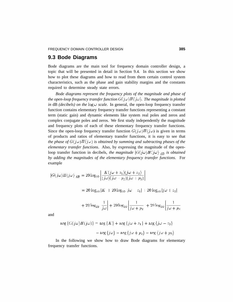
9.3.1 Phase and Gain Stability Margins from Bode DiagramsIt hasbeenalreadyindicatedin Figure9.1how to readthephaseandgainstabilitymarginsfrom thefrequencymagnitudeandphaseplotsof theopen-loopfeedbacktransferfunction. In the caseof Bodediagramsthe magnitudeplot is expressedin �� (decibels)so that the gain crossoverfrequencyis obtainedat the pointof intersectionof the Bode magnitudeplot and the frequencyaxis. Bearinginmind the definition of the phaseand gain stability margins given in (4.54) and(4.55), and the correspondingphaseand gain crossoverfrequenciesdefinedin(4.56) and (4.57), it is easyto concludethat thesemargins can be found fromBode diagramsas indicatedin Figure 9.9.

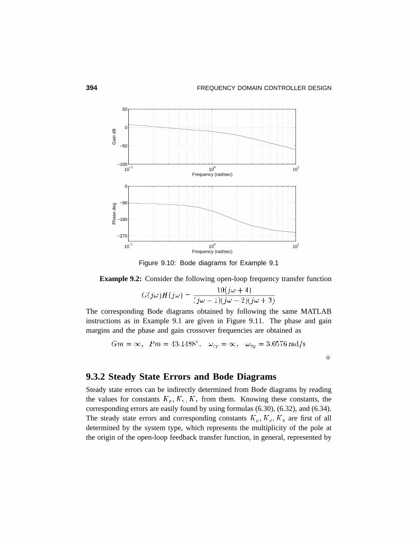
Example 9.1: In this examplewe useMATLAB to plot Bodediagramsforthe following open-loopfrequencytransferfunctionüLý2þ.ÿ+�-, ý!þ.ÿ �� ý!þ.ÿ.�/�0�þ.ÿ ýgþ.ÿ1�2�(��3!ý2þ.ÿ � � �2��ýgþ.ÿ �4�5�76Bodediagramsareobtainedby usingtheMATLAB functionbode(num,den) .Thephaseandgainstabilitymarginsandthephaseandgaincrossoverfrequenciescan be obtainedby using [Gm,Pm,wcp,wcg]=margin(num,den) . Notethat the open-loopfrequencytransferfunction has to be specifiedin terms ofpolynomialsnum (numerator)and den (denominator).The MATLAB functionconv helpsto multiply polynomialsasexplainedbelow in the programwrittento plot Bodediagramsandfind the phaseandgain margins for Example9.1.


(a)80

í20log Kp

(b)

ω9 cg

ω9 cg

ω9 cp logω

logωω9 cp

-180o

-90o

0í o

G(jω)H(jω)

arg: G(jω)H(jω)

Pm

-Gm

dBì

Figure 9.9: Gain and phase margins and Bode diagrams

num=[1 1];d1=[1 0];d2=[1 2];d3=[1 2 2];den1=conv(d1,d2);den=conv(den1,d3);bode(num,den);[Gm,Pm,wcp,wcg]=margin(num,den);

The correspondingBodediagramsarepresentedin Figure9.10. The phaseand gain stability margins and the correspondingcrossoverfrequenciesare ob-tained as;=<?>A@�BDC7E�E�F�GIHKJ�L�<M>N@'O�BPO0E0Q�O7R7J�SUTWV�>YX'BPZ7C�@'C�[]\�GI^!_`J�SaTcb�>ed�BfO!g�g'@�[]\'GI^!_h


10−1

100

101

−100

−50

0

50

Frequency (rad/sec)

Gai

n dB

10−1

100

101

−90

−180

−270

0

Frequency (rad/sec)

Pha

se d

eg

Figure 9.10: Bode diagrams for Example 9.1

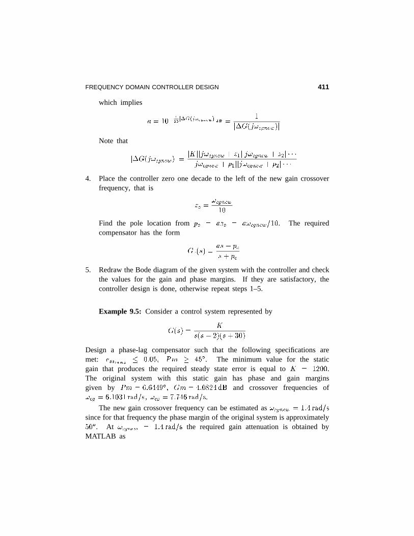
Example 9.2: Considerthe following open-loopfrequencytransferfunctionikjcl7m�npoqjrl'm+nUs t&u jrl'm.vxwynjcl'mzv t n{jrl'm.v5|}n~jrl'mzv2�(nThe correspondingBode diagramsobtainedby following the sameMATLABinstructionsas in Example9.1 are given in Figure 9.11. The phaseand gainmargins and the phaseandgain crossoverfrequenciesareobtainedasi��?se�A�5��?s/w(�� t w0��7��ma�c��se�A�?ma�c��sN�� u!�(�!��~��$� �9.3.2 Steady State Errors and Bode DiagramsSteadystateerrorscanbe indirectly determinedfrom Bodediagramsby readingthe valuesfor constants� � � �k� � �� from them. Knowing theseconstants,thecorrespondingerrorsareeasilyfoundby usingformulas(6.30),(6.32),and(6.34).The steadystateerrorsand correspondingconstants� �� are first of alldeterminedby the systemtype, which representsthe multiplicity of the pole attheorigin of theopen-loopfeedbacktransferfunction, in general,representedby


10−2

10−1

100

101

102

−100

−50

0

50

Frequency (rad/sec)

Gai

n dB

10−2

10−1

100

101

102

−90

−180

0

Frequency (rad/sec)

Pha

se d

eg

Figure 9.11: Bode diagrams for Example 9.2

��r�'�� q�c�'� �U¡ ¢ �£�'�.¤2¥$¦§�{�c�'�.¤¥§¨&�ª©$©§©�c�'�+� «§�r�'�z¤¬ ¦ �{�c�'�.¤®¬ ¨ �¯©§©$© (9.16)

This can be rewritten as�°�£�'��p�x�£�'�+�U¡ ¢ ¥ ¦ ¥ ¨ ©$©§©�±�²+¤´³pµ¶¸·!¹ ±�² ¤´³pµ¶pº(¹ ©§©$©¬ ¦ ¬ ¨ ©$©§©~�c�'�+�»«I±�² ¤e³{µ¼ ·7¹ ±�²+¤A³pµ¼ º'¹ ©$©§©¡ ¢�½ ± ²+¤ ³pµ¶ · ¹ ± ²+¤ ³pµ¶ º ¹ ©$©§©�r�'�+� «I± ² ¤ ³{µ¼ · ¹ ± ² ¤ ³{µ¼ º ¹ ©$©§©

(9.17)

where ¢¾½ ¡ ¢ ¥ ¦ ¥ ¨ ©$©§©¬ ¦ ¬ ¨ ©§©$© (9.18)

is known asBode’sgain, and ¿ is the type of feedbackcontrol system.


For controlsystemsof type À�ÁAÂ , thepositionconstantaccordingto formula(6.31) is obtainedfrom (9.17) asÃ°Ä Á ÃkÅ�Æ�Ç+È´ÉpÊË~Ì�Í Æ(Ç ÈAÉ{ÊËÏÎ'Í�Ð§Ð$ÐÑrÒ0Ó�Ô»Õ Æ�Ç+ÈeÉ{ÊÄ Ì$Í Æ�Ç+ÈeÉpÊÄ Î0Í�Ð$Ð§Ð�Ö ÉpÊ�× Õ Á Ã Å (9.19)

It follows from (9.17)–(9.19)that the correspondingmagnitudeBodediagramoftypezerocontrolsystemsfor smallvaluesof

Óis flat (hasaslopeof Â�ØIÙ ) andthe

valueof Ú�Â�Û£Ü�Ý Ã¾Å ÁAÚ�Â�ÛcÜ�Ý Ã Ä . This is graphicallyrepresentedin Figure9.12.

log ω

|G(jω)H(jω)|dB

20logKp

Figure 9.12: Magnitude Bode diagram of typezero control systems at small frequencies

For control systemsof type Þ�ß�à , theopen-loopfrequencytransferfunctionis approximatedat low frequenciesbyá¾â�ã à+äAåpæç~è(é ã à+äeåpæç{ê(é�ë$ë$ëì£í'î�ï-ð ã à+äAå{æñ è!é ã à ä´åpæñ ê7é�ë§ë$ëªò á¾âì£í'î�ï{ð (9.20)

It follows that the correspondingmagnitudeBode diagramof type one controlsystemsfor small valuesof

îhasa slopeof óõô�öU÷�ø+ù7÷(ú!û&ü�÷}ú andthe valuesofô�ö�ýcþ�ÿ�� á¾âí�� ßNô�ö�ýcþ�ÿ�� á¾â �!ó5ô'ö�ýrþ'ÿ�� î � (9.21)

From (9.20) and (6.33) it is easyto concludethat for type one control systemsthe velocity constantis

á�� ß á¾â. Using this fact and the frequencyplot of


(9.21),we concludethat � is equalto the frequency� � at which the line (9.21)intersectsthe frequencyaxis, that is�� ! "� � � � � " (9.22)

This is graphically representedin Figure 9.13.

log ω

|G(jω)H(jω)|dB |G(jω)H(jω)|dB

ω=1

ω=1

ω# * =Kv

ω# * =Kv log ω

K$

v <1

-20 dB/dec-20 dB/dec

Kv >1

(a) (b)

20logKv

20logKv

Figure 9.13: Magnitude Bode diagram of typeone control systems at small frequencies

Note that if %"&('*),+(-/. , the correspondingfrequency ) + is obtainedat thepoint where the extendedinitial curve, which has a slope of 0�1�24365�78369;:=<�3�9 ,intersectsthe frequencyaxis (seeFigure 9.13b).

Similarly, for type two control systems,>�'�1 , we haveat low frequencies%"?A@�.,BDCFEGIH8J @�. BKCLEGLMNJPO;OQORTS )�UWVX@�.,BDCLEY HQJ @Z.,B[CLEY M�JPO;O;O]\ % ?R�S ),ULV (9.23)

which indicatesaninitial slopeof 0,^Z2_365`7�3�9;:=<�3N9 andafrequencyapproximationof 1�2�aTb�cedddd %"?R�S�f U V dddd '�1�2gaTb�c�h %"?�h�0i1�2gaTb�c dd ) V dd '�1�2�aTb�cjhk%"?�hQ0l^N2�aTb�cm) (9.24)

From (9.23) and(6.35) it is easyto concludethat for type two control systemsthe accelerationconstantis %onp'q%"? . From the frequencyplot of the straightline (9.24), it follows that %"?r' R ) +s+QUWV , where ) +s+ representsthe intersectionof


the initial magnitudeBodeplot with the frequencyaxis as representedin Figure9.14.

log ω

|G(jω)H(jω)|dB

|G(jω)H(jω)|dB

ω=1

ω=1 log ω

-40 dB/dec -40 dB/dec

(a) (b)

20logKa

20logKa

ω** = Ka

ω** = Ka

Figure 9.14: Magnitude Bode diagram of typetwo control systems at small frequencies

It can be seenfrom Figures 9.12–9.14that by increasingthe values forthe magnitudeBode diagramsat low frequencies(i.e. by increasing t�u ), theconstantstAvZwxtAy , and t�z are increased.According to the formulasfor steadystateerrors,given in (6.30), (6.32), and (6.34) as{�|}|F~��T�`� ��,� t v w {;|}|s�T��Z�� t y w {Q|W|}��F�T�F��T��_� �t zwe concludethat in this casethe steadystateerrors are decreased.Thus, thebigger t"u , the smaller the steadystateerrors.

Example 9.3: ConsiderBode diagramsobtainedin Examples9.1 and 9.2.The Bodediagramin Figure9.10 hasan initial slopeof � �8��6�`��;�=��N� whichintersectsthe frequencyaxis at roughly � � � �6�� I��X��¡ . Thus,we havefor theBode diagramin Figure 9.10t v �D¢ w£t y�¤ �6�� w t z � �Using the exactformula for t y , given by (6.33), we gett y �K¥�¦T§|W¨�©4ª�« ¬ « ��8®« ¬ « �r��® ¬ «;¯ �°� « �°�N®6± � �6��²


In Figure9.11 the initial slopeis ³�´6µ , andhencewe havefrom this diagram¶ ³¸·T¹�º »p¼�½!¾;¿ÁÀ »p¼�½�¿6Â�Ã ¶6Ä »�ÅÇÆ�³ Ä »"È�Æ�³Using the exactformula for »p¼ as given by (6.31) produces» ¼ ÆD·�ÉTÊË}Ì�Í�Î ¾;³�ÏLÐ`ÑiÒ6ÓÏLÐ,Ñ[¾8ÓFÏLÐ`Ñ ¶ ÓsÏFÐ,ÑÕÔNÓ6Ö Æ×Ã�Â�Ã�ØNotethattheaccurateresultsaboutsteadystateerrorconstantsareobtainedeasilyby usingthecorrespondingformulas;hencetheBodediagramsareusedonly forquick and rough estimatesof theseconstants. Ù9.4 Compensator Design Using Bode Diagrams

In this sectionwe showhow to useBodediagramsin orderto designcontrollerssuchthat theclosed-loopsystemhasthedesiredspecifications.Threemain typesof controllers—phase-lead,phase-lag,andphase-lag-leadcontrollers—havebeenintroducedin the time domain in Chapter8. Here we give their interpretationin the frequencydomain.

We presentthedesignprocedurefor thegeneralcontrollersmentionedabove.Similar andsimplerprocedurescanbedevelopedfor PD,PI, andPID controllers.After masteringthe designwith phase-lead,phase-lag,and phase-lag-leadcon-trollers, studentswill be able to proposetheir own algorithmsfor PD, PI, andPID controllers.

Controller designtechniquesin thefrequencydomainwill begovernedby thefollowing facts:

(a) Steadystateerrors are improvedby increasingBode’sgain »�Ú .(b) Systemstability is improvedby increasingphaseand gain margins.(c) Overshootis reducedby increasingthe phasestability margin.(d) Risetime is reducedby increasingthe system’sbandwidth.

However, very often it is not possibleto satisfy all of theserequirementsatthe same time, and control engineershave to compromisebetweenseveralcontradictingrequirements.


The first two items, (a) and (b), have beenalreadyclarified. In order tojustify item (c), we considerthe open-looptransferfunction of a second-ordersystemgiven by ÛpÜTÝ8Þ�ßLàáÜ�Ý�Þ�ß4â Þ ãäÜTÝ�Þ`ßFÜTÝ�å°ærç�èQÞ ä ß (9.25)

whosegain crossoverfrequencycan be easily found fromé ÛpÜ�Ý�Þ�êìëZßWàáÜTÝ�Þ4êìë�ß é â Þ ãäÞ�í Þ ã ærîNè ã Þ ãä â!ï(9.26)

leading to Þ4êìëðâÞ äòñ í ïóæiîZè ã�ô ç�è ã (9.27)

The phaseof (9.25) at the gain crossoverfrequencyisõ;öø÷�ù ÛpÜ�Ý�Þgêìë�ßLàiÜ�Ý�Þgêìë�ßsúðâ ô�û�ü�ý,ôiþ õ;ÿ�� Þgêìëç�èQÞ ä (9.28)

so that the correspondingphasemargin becomes�� â þ õ8ÿ � � ç�èñ í ï,æ�îZè ã ô ç�è ã

â �� ÜLè�ß(9.29)

Plottingthefunction�� Ü�è�ß

, it canbeshownthatit is a monotonicallyincreasingfunction with respectto

è; we thereforeconcludethat the higherphasemargin,

the larger the dampingratio, which impliesthe smaller the overshoot.

Item (d) cannotbe analytically justified sincewe do not havean analyticalexpressionfor the responserise time. However, it is very well known fromundergraduatecourseson linearsystemsandsignalsthatrapidly changingsignalshavea wide bandwidth.Thus,systemsthat are able to accommodatefastsignalsmusthavea wide bandwidth.

In the remainderof this section,we first presentstandardcontrollers(phase-lag, phase-lead,andphase-lag-lead)in thefrequencydomain,andthenshowhowto usethesein order to achievethe desiredsystemspecifications.Eachdesigntechniquewill be given in an algorithmic form, and eachwill be demonstratedby an example.


9.4.1 Phase-Lag ControllerThe transferfunction of a phase-lagcontroller is given by�� ! �"�� "� �$# ��%&('# � %) '+* � ��,-�� (9.30)

The correspondingmagnitudeand phasefrequencydiagramsfor a phase-lagcontroller are presentedin Figure 9.15.

log ω

log ωω. max

φ/

max

20log(p1 / z1)

p0 1

0

01

z1

|2Gc(jω)|

dB

arg{3 Gc(jω)}

Figure 9.15: Magnitude approximation and exact phase of a phase-lag controller

Notethatfor themagnitudediagramit is sufficient to useonly thestraightlineapproximationsfor a completeunderstandingof the role of this controller. Ingeneral,straightlineapproximationscan be usedfor almostall Bode magnitudediagramsin controllerdesignproblems.However,phaseBodediagramsareverysensitiveto changesin frequencyin the neighborhoodof the cornerfrequencies,and so shouldbe drawn as accuratelyas possible.

Due to attenuationof the phase-lagcontroller at high frequencies,thefrequencybandwidthof thecompensatedsystem(controllerandsystemin series)is reduced. Thus, the phase-lagcontrollers are usedin order to decreasethe


systembandwidth(to slow downthe systemresponse).In addition, they can beusedto improvethe stability margins (phaseand gain) while keepingthe steadystateerrors constant.

Expressionsfor 465�798 and :;5<7=8 of a phase-lagcontrollerwill be derivedinthe next subsectionin the contextof the studyof a phase-leadcontroller. As amatterof fact, both typesof controllershavethe sameexpressionsfor thesetwoimportant designquantities.

9.4.2 Phase-Lead ControllerThe transferfunction of a phase-leadcontroller is>�?@ 7BA�CED"4�F�G�H�I�JK J�L K J!M D"4I;JNM D"4 G�O M D�PQSRO M DTPUVR�W I�JTX K J (9.31)

andthe correspondingmagnitudeandphaseBodediagramsareshownin Figure9.16.

log ω

logY

ωωZ max

φ[

max

20log(p2/z2 )

p\ 20]

0]

z^ 2|_Gc(jω)|

dB

arg{` Gc(jω)}

Figure 9.16: Magnitude approximation and exact phase of a phase-lead controller

Due to phase-leadcontroller (compensator)amplificationat higher frequencies,it increasesthebandwidthof thecompensatedsystem.Thephase-leadcontrollers


areusedto improvethegainandphasestabilitymarginsandto increasethesystembandwidth(decreasethe systemresponserise time).

It follows from (9.31) that the phaseof a phase-leadcontroller is given byacb(d�egf�hikjBlnm�o"p�q9rtsvuBa�wyx+zT{ p|�}�~�� uBa�wyx�z�{ p� }�~ (9.32)

so that �� p a�b=d�e�fth�ikjBlnmEo"p�q=r�s�� p6� j=� s�� | } � } (9.33)

Assumethat � }�s��|c}�� p � j(� s � }� � (9.34)

Substituting p � j=� in (9.32) impliesu�a�w�� j(� s � � �� (9.35)

It is left as an exercisefor studentsto give detailed derivationsof formula(9.35)—seeProblem9.3.

It is easyto find, from (9.35), that the value for parameter� in terms of� � j(� is given by ��s �<��w � � j(�� w � � j(� (9.36)

Note that the sameformulasfor p � j=� , (9.33), and the parameter� , (9.36),hold for a phase-lagcontroller with � z ��| z replacing � }��|c} and with � z s¡��| z ��£¢¤� .9.4.3 Phase-Lag-Lead ControllerThe phase-lag-leadcontrollerhasthe featuresof both phase-lagand phase-leadcontrollersand can be usedto improve both the transientresponseand steadystateerrors. However,its designis more complicatedthan the designof either


phase-lagor phase-leadcontrollers.Thefrequencytransferfunctionof thephase-lag-leadcontroller is given by¥t¦(§�¨"©�ª�« §�¨"©¬¯®c°nª(§�¨"©±¬²®c³nª§�¨"©´¬¶µ;°nª=§�¨"©±¬µ�³nª « ®c°·®n³µ�°9µ;³¹¸�º ¬±¨¼»½�¾B¿ ¸�º ¬±¨�»½=ÀÁ¿¸Âº ¬¶¨T»Ã ¾B¿ ¸�º ¬±¨T»Ã À·¿« ¸ º ¬±¨�»½ ¾·¿ ¸ º ¬¨�»½ Àc¿¸ º ¬¨�»Ãc¾B¿ ¸ º ¬¨T»ÃVÀÁ¿tÄ ®n°·®c³T«�µ;°9µ�³ Ä µ�³�ÅÆ®c³TÅ�®n°TÅ�µ;° (9.37)

The Bode diagramsof this controller areshownin Figure 9.17.

log ω

log ω

pÇ 1 pÇ 2

0

0È

zÉ 1 z2

|ÊGc(jω)|

dB

arg{Ë Gc(jω)}

Figure 9.17: Bode diagrams of a phase-lag-lead controller

9.4.4 Compensator Design with Phase-Lead ControllerThe following algorithm can be usedto designa controller (compensator)witha phase-leadnetwork.


Algorithm 9.1:

1. Determinethe valueof the Bode gain Ì�Í given by (9.18) asÌ�Í¯Î Ì±ÏnÐ·ÏcÑ�ÒnÒcÒÓ Ð Ó Ñ ÒnÒcÒsuchthat the steadystateerror requirementis satisfied.

2. Find the phaseandgainmarginsof the original systemwith Ì�Í determinedin step 1.

3. Find thephasedifference,ÔÖÕ , betweentheactualanddesiredphasemarginsandtake Õ;×<Ø=Ù to be Ú�Û – ÜcÝ"Û greaterthanthis difference.Only in rarecasesshouldthis be greaterthan ÜcÝ Û . This is dueto the fact that we haveto giveanestimateof a newgaincrossoverfrequency,which cannot bedeterminedvery accurately(seestep 5).

4. Calculatethe valuefor parameterÞ from formula (9.36), i.e. by usingÞ�Î Ü<ß²à�áEâ Õ;×ãØ(ÙÜ�äåà�á�â�Õ;×ãØ(Ù�æ Ü5. Estimatea valuefor a compensator’spolesuchthat ç6×<Ø=Ù is roughly located

at the new gain crossoverfrequency,çè×ãØ(Ùêéëçíìïî�ð�ñóò . As a rule of thumb,add the gain of ÔÖôõÎ÷ö�ÝÁø�ù�úüûSÞ�ýBþÿ�� at high frequenciesto the uncompen-satedsystemand estimatethe intersectionof the magnitudediagramwiththe frequencyaxis,say çíÐ . Thenewgaincrossoverfrequencyis somewherein betweenthe old ç�ìïî and çíÐ . Someauthors(Kuo, 1991) suggestfixingthe new gain crossoverfrequencyat the point where the magnitudeBodediagramhas the value of ä Ý��Ú"ÔÖô�þ ÿ�� . Using the value for parameterÞobtainedin step 4 find the value for the compensatorpole from (9.34) asä Ó ìTÎ ä�ç6×<Ø=Ù�� Þ and the value for compensator’szero as äTÏnì�Î ä Ó ìgÞ .Note that onecanalsoguessa valuefor Ó ì and thenevaluateÏnì and çè×ãØ(Ù .The phase-leadcompensatornow can be representedbyô ì û��ýNÎ Þ��¼ß Ó ì�¼ß Ó ì

6. Draw the Bode diagramof the given systemwith controller and checkthevaluesfor thegainandphasemargins. If theyaresatisfactory,thecontrollerdesignis done,otherwiserepeatsteps1–5.


The next exampleillustratescontrollerdesignusingAlgorithm 9.1.

Example 9.4: Considerthe following open-loopfrequencytransferfunction

�� "!��#�%$&�'��(�")*��#�,+��Step1. Let the designrequirementsbesetsuchthat the steadystateerror duetoa unit stepis lessthan2% andthe phasemargin is at least -/.�0 . Since

13242 � $$�� 65 � $$�� 798 �:7 � �<; !$ ; ) ; + � �we concludethat �>= .@? will satisfythe steadystateerror requirementof beingless than 2%. We know from the root locus techniquethat high static gainscandamagesystemstability, andso for the restof this designproblemwe take� � .@? .Step2. We drawBodediagramsof theuncompensatedsystemwith theBodegainobtainedin step1 and determinethe phaseandgain margins and the crossoverfrequencies. This can be done by using the following sequenceof MATLABfunctions.

[den]=input(’enter denominator’);% for this example [den]=[1 6 11 6];[num]=input(’enter numerator’);% for this example [num]=[50 300];[Gm,Pm,wcp,wcg]=margin(num,den);bode(num,den)

The correspondingBode diagramsare presentedin Figure 9.18a. The phaseand gain margins are obtainedas

BAC�ED 8 F AG� .�HI.@J�0 and the crossoverfrequenciesare

�LKNMO�QP HR.�- )�+TSVU�WYX�Z 8 �LK 5 �QD .

Step3. Since the desiredphaseis well above the actual one, the phase-leadcontroller must make up for -/.@0\[].�HR.@J@0 �^+ J�H_- $ 0 . We add

$ ?@0 , for thereasonexplainedin step3 of Algorithm 9.1, so that `ba�c'd � -/J�He- $ 0 . The aboveoperationscan be achievedby using MATLAB as follows


10−1

100

101

102

−50

0

50

Frequency (rad/sec)

Gai

n dB

10−1

100

101

102

−90

−180

0

Frequency (rad/sec)

Pha

se d

eg

(a)

(a)

(b)

(b)

Figure 9.18: Bode diagrams for the original system(a) and compensated system (b) of Example 9.4

% estimate Phimax with Pmd = desired phase margin ;Pmd=input(’enter desired value for phase margin’) ;Phimax=Pmd-Pm+10 ;% converts Phimax into radians ;Phirad=(Phimax/180)*pi ;

Step4. Here we evaluatethe parameterf accordingto the formula (9.36) andget fhgji/kIl�mon@n . This can be donein MATLAB by

a=(1+sin(Phirad))/(1–sin(Phirad)) ;

Step5. In order to obtain an estimatefor the new gain crossoverfrequencywe first find the controller amplificationat high frequencies,which is equal top@qsr�t�u�v fxw�gym&i/k p�z l@{}|b~]g��\�B�'� . The magnitudeBode diagramincreasedby�:� �� at high frequenciesintersectsthe frequencyaxis at �}��Qm q k ��V�@|b�� .We guess(estimate)the value for �� as �b��g p � , which is roughly equal to� ��@� f . By using � � g p � andforming the correspondingcompensator,we getfor thecompensatedsystem�B��g�n z k p@z�� m�� at �}�N�V @¡£¢ g]m�l�k z �xm � �¤�@|b�� , whichis satisfactory.This stepcan be performedby MATLAB as follows.


% Find amplification at high frequencies, DG;DG=20*log10(a) ;% estimate value for pole —pc from Step 5;pc=input(’enter estimated value for pole pc’) ;% form compensator’s numerator ;nc=[a pc] ;% form compensator’s denominator ;dc=[1 pc] ;% find the compensated system transfer function ;numc=conv(num,nc) ;denc=conv(den,dc) ;[Gmc,Pmc,wcp,wcg]=margin(numc,denc) ;bode(numc,denc)

The phase-leadcompensatorobtainedis given by¥§¦�¨�©�ª}«Q¬/R®�¯¤°@° ©�±"²@³©�±,²@³ «j´ ©�±#µ·¶©�±#µ ¶Step6. The Bodediagramsof the compensatedcontrol systemarepresentedinFigure9.18b. Both requirementsaresatisfied,andthereforethecontrollerdesignprocedureis successfullycompleted.

It is interesting to comparethe transient responsecharacteristicsof thecompensatedanduncompensatedsystems.Thiscannotbeeasilydoneanalyticallysince the orders of both systemsare greaterthan two, but it can be simplyperformedby using MATLAB. Note that num, den , numc, denc represent,respectively,thenumeratorsanddenominatorsof theopen-looptransferfunctionsof the original and compensatedsystems. In order to find the correspondingclosed-looptransferfunctions,we usethe MATLAB function cloop , that is

[cnum,cden]=cloop(num,den,-1);% —1 indicates a negative unit feedback[cnumc,cdenc]=cloop(numc,denc,-1);

The closed-loopstepresponsesare obtainedby

[y,x]=step(cnum,cden);[yc,xc]=step(cnumc,cdenc);

and are representedin Figure 9.19. It can be seenfrom this figure that boththe maximumpercentovershootandthe settling time aredrasticallyreduced.In


addition, the rise time of the compensatedsystemis shortenedsincethe phase-lead controller increasesthe frequencybandwidthof the system.

0 0.2 0.4 0.6 0.8 1 1.2 1.4 1.6 1.8 20

0.2

0.4

0.6

0.8

1

1.2

1.4

1.6

1.8

2

(a)

(b)

Figure 9.19: Step responses for the original (a) and compensated (b) systems

The highly oscillatorybehaviorof the stepresponseof the original systemcanbe fully understoodfrom its root locus,which is given in Figure9.20. It canbe seenthat the real part of a pair of complexconjugatepolesis very small foralmostall valuesof the staticgain,which causeshigh-frequencyoscillationsandvery slow convergenceto the responsesteadystatevalue.

The closed-loopeigenvaluesof the original and compensatedsystems,ob-tainedby MATLAB functionsroots(cden) androots(cdenc) , aregivenby ¸*¹»º]¼¾½�¿IÀ@Á@Â�Â/ÃÄ¸·ÅÆ ÇÈºÉ¼�Ê�¿RÀ@À@½�ËÍÌ#Î�Ï�¿I½*Ï�Ê�Ð¸·¹¤Æ Å'Ñ�ºÉ¼�Ò�¿RË�Ï�À@Ë�Ì#ÎbÓ�À�¿RÀ@Ò�Â@ÒxÃ�¸�ÇVÑ�ºÉ¼»Â�¿IÁ�Ë@Á�Â�Ã(¸�ÔVÑ�ºÉ¼»À�¿RÀ@Ò�Ê@Êwhich indicatesa big differencein the real partsof complexconjugatepolesforthe original and compensatedsystems. Õ


−10 −5 0 5 10

−10

−5

0

5

10

Real Axis

Imag

Axi

s

Figure 9.20: Root locus of the original system

9.4.5 Compensator Design with Phase-Lag ControllerCompensatordesignusing phase-lagcontrollersis basedon the compensator’sattenuationat high frequencies,which causesa shift of the gain crossoverfrequencyto the lower frequencyregion where the phasemargin is high. Thephase-lagcompensatorcan be designedby the following algorithm.

Algorithm 9.2:

1. Determinethevalueof theBodegain Ö:× thatsatisfiesthesteadystateerrorrequirement.

2. Find on the phaseBode plot the frequencywhich has the phasemarginequal to the desiredphasemargin increasedby Ø@Ù to Ú�Û�Ù . This frequencyrepresentsthe new gain crossoverfrequency,ÜLÝ�Þ¤ß�à£á .

3. Read the required attenuationat the new gain crossoverfrequency, i.e.â ã:ä�åçæ Ü ÝNÞVß�à£á�è â é × , and find the parameterê fromë¾ì Ûsí�î�ï ðòñ·óô ó�õ÷ö ë»ì Ûøí�î�ï å ê è ö â_ã\ä6å�æ Ü ÝNÞVß�à£á è â é ×


which implies ù�úüûþý�ÿ��

ú û� ��! #"%$'&)(+*�,�-/.0�

Note that

� ��! #"1$/&)(+*�,�-2.3�ú � 45�6� "1$/&)(+*�,�-87:9<;1�=� "1$/&)(+*�,�->7?9<@1�+ABA<A� "1$ &)(+*�,�- 7DC ; �6� "1$ &)(E*�,�- 7>C @ �+A<A<A

4. Placethe controller zero one decadeto the left of the new gain crossoverfrequency,that is 9B&

ú $F&)(+*%,�-û3ýFind the pole location from

C &ú ù

9 &ú ù

$ &)(+*�,�-HGû�ý

. The requiredcompensatorhas the form

� & �I�.ú ù IJ7DCK&IJ7>CL&

5. RedrawtheBodediagramof the givensystemwith the controllerandcheckthe values for the gain and phasemargins. If they are satisfactory,thecontroller designis done,otherwiserepeatsteps1–5.

Example 9.5: Considera control systemrepresentedby

�! �I�.ú 4I% IM7?N1.O �IP7?Q

ý.

Design a phase-lagcompensatorsuch that the following specificationsaremet: R<S�SUT6V WYX[Z

ý\ý]_â`cb d e_]gf

. The minimum value for the staticgain that producesthe required steady state error is equal to

4ú û

Ný@ý

.The original system with this static gain has phase and gain marginsgiven by

`hbúi \ i%ege�j f ^ � b

úe \ýk N eHlYm

and crossover frequencies of$ &)(úi \û�ýQûn+o l GBp ^ $ &6q

úr \ r<esi n+o l G%p .

The new gain crossoverfrequencycan be estimatedas$F&)(+*%,�-

ú û\ e n+o l G�p

sincefor that frequencythephasemargin of theoriginal systemis approximately]ýf. At

$F&)(E*�,�-ú û

\ e nEo l G%p the required gain attenuationis obtained byMATLAB as


wcgnew=1.4;d1=1200;g1=abs(j*1.4);g2=abs(j*1.4+2);g3=abs(j*1.4+30);dG=d1/(g1*g2*g3);

which producest�u�vxw6y{zg| }Y~3t{��zgzg|��g�g�1� and ��z��Yt u�vxw�y{zg|�}_~3tY��Y|��%�g�g� . Thecompensator’spole and zero are obtainedas ��B��F��E��szB��Y|)z3} and�'� � �� )�+�%�� szB��[��|��zE 1� (seestep4 of Algorithm 9.2). The transferfunction of the phase-lagcompensatoris

vc�Ow�¡�~'� �Y|¢�g�1�g�1¡2£:�Y|��z< 1�¡P£?��|��z< 1�TheBodediagramsof the original andcompensatedsystemsaregiven in Figure9.21.

10−1

100

101

102

−100

−50

0

50

Frequency (rad/sec)

Gai

n dB

10−1

100

101

102

−90

−180

−270

0

Frequency (rad/sec)

Pha

se d

eg

(a)

(a)

(b)

(b)

Figure 9.21: Bode diagrams for the original system(a) and compensated system (b) of Example 9.5

The new phaseand gain margins and the actual crossoverfrequenciesare¤c¥�¦J§5¨�©sª�«g¬%, ® ¥�¦M§°¯�¨Lª�±1¯F²Y³

, ´Fµ)¶+·%¸�¹ §»º1ª�¨s«1¼¾½U¿g²ÁÀBÂ, ´/µ�Ã+·�¸�¹ §Ä©_ª�¨�©g©¾½+¿g²ÁÀ�Â

andso the designrequirementsare satisfied. The stepresponsesof the original


and compensatedsystemsare presentedin Figure 9.22.

0 1 2 3 4 5 6 7 8 9 100

0.2

0.4

0.6

0.8

1

1.2

1.4

1.6

1.8

2

Time (secs)

Am

plitu

de(a)

(b)

Figure 9.22: Step responses for the original system(a) and compensated system (b) of Example 9.5

It canbeseenfrom this figure that theovershootis reducedfrom roughly0.83to0.3. In addition, it can be observedthat the settling time is also reduced.Notethat the phase-lagcontroller reducesthe systembandwidth(ÅFÆ)Ç+ÈgÉ�Ê�ËÌÅ/Æ)Ç ) sothat the rise time of the compensatedsystemis increased.

Í9.4.6 Compensator Design with Phase-Lag-Lead ControllerCompensatordesignusingaphase-lag-leadcontrollercanbeperformedaccordingto the algorithmgiven below, in which we first form a phase-leadcompensatorand thena phase-lagcompensator.Finally, we connectthem togetherin series.Note that severaldifferent algorithms for the phase-lag-leadcontroller designcan be found in the control literature.

Algorithm 9.3:

1. Seta valuefor thestaticgain Î�Ï suchthatthesteadystateerrorrequirementis satisfied.

2. Draw Bodediagramswith Î�Ï obtainedin step1 andfind thecorrespondingphaseand gain margins.


3. Find the difference between the actual and desired phase margins,Ð�Ñ�ÒÔÓcÕ�ÖØ×�ÓhÕ, and take

ÑKÙPÚUÛto be a little bit greaterthan

Ð�Ñ. Cal-

culatethe parameterÜ_Ý of a phase-leadcontrollerby using formula (9.36),that is

Ü_Ý ÒßÞPà:á�â#ã Ñ ÙHÚOÛÞ × á�â�ã Ñ ÙHÚOÛ4. Locatethe new gain crossoverfrequencyat the point whereä�åFæ#ç%èhé ê!ë#ì%í'î)ï+ð%ñóò2ô3é Ò»× Þ å�æ#ç1è Ü_Ý (9.38)

5. Computethe valuesfor the phase-leadcompensator’spole andzerofrom

õ î Ý Ò íFî)ï+ð%ñ�ò'ö Ü_Ý%÷ ø î Ý Ò õ î ÝBù%ÜsÝ (9.39)

6. Selectthe phase-lagcompensator’szeroand pole accordingto

ø î�ú Ò åYû Þ ø î Ý%÷ õ î�ú Ò ø î�ú ù%Ü_Ý (9.40)

7. Form the transferfunction of the phase-lag-leadcompensatoras

êcîOë�ü�ô Ò êcý Ú ï%ë�ü�ôHþ>êØý�ñ Ú+ÿ ë�ü�ô Ò ü à ø î�úü à õ î�ú þü à ø î Ýü à õ î Ý

8. PlotBodediagramsof thecompensatedsystemandcheckwhetherthedesignspecificationsare met. If not, repeatsomeof the stepsof the proposedalgorithm—in most casesgo back to steps3 or 4.

The phase-leadpart of this compensatorhelpsto increasethe phasemargin(increasesthedampingratio, which reducesthemaximumpercentovershootandsettling time) and broadenthe system’sbandwidth(reducesthe rise time). Thephase-lagpart, on the otherhand,helpsto improve the steadystateerrors.

Example 9.6: Considera control systemthat has the open-looptransferfunction ê!ë ü%ô Ò � ëóü àÔÞ å1ôë�ü Ý à ägü à ä_ô ë ü à ägå ôFor this systemwe designa phase-lag-leadcontroller by following Algorithm9.3 suchthat the compensatedsystemhasa steadystateerror of lessthan 4%and a phasemargin greaterthan � å�� . In the first step,we choosea value for


the staticgain � that producesthe desiredsteadystateerror. It is easyto checkthat �� , andthereforein the following we stick with thisvalue for the static gain. Bode diagramsof the original systemwith ��are presentedin Figure 9.23.

10−1

100

101

102

−50

0

50

Frequency (rad/sec)

Gai

n dB

Gm=Inf dB, (w= NaN) Pm=31.61 deg. (w=7.668)

10−1

100

101

102

0

−90

−180

−270

−360

Frequency (rad/sec)

Pha

se d

eg

Figure 9.23: Bode diagrams of the original system

It can be seenfrom thesediagrams—andwith help of MATLAB determinedaccurately—thatthe phaseand gain margins and the correspondingcrossoverfrequenciesare given by �! "�#�$�%'&�$)(�*,+- "/. , and 021435"/67%'&�&�8:9,;�<>=�?)*0 1A@ "�. . According to step3 of Algorithm 9.3, a controller hasto introducea phaselead of $B8�%C#ED ( . We take F>GIHKJL"NM�O ( and find the requiredparameterP�Q "RMS%�T7&�#�D . Taking 0 1U3)VEWYX "�M�Z[9,;�\]=E? in step4 and completingthe designsteps5–8 we find that �! �"^#�D�%CD�T ( , which is not satisfactory.We go back tostep3 and take F>GIHKJ_"`#�Z ( "�Z�%'O�M�#�&29,;�\ , which implies P�Q "�# .

Step4 of Algorithm 9.3 can be executedefficiently by MATLAB by per-forming the following search. Since a-$Z:b4c�dI#e"fa-$BZ�%'D�8�&S$g\�h we searchthemagnitudediagram for the frequencywhere the attenuationis approximatelyequalto ai$�$j\�h . We startsearchat 0k"lM�Zm9,;�\>=�? sinceat that point, accordingto Figure9.23,theattenuationis obviouslysmallerthan a-$�$i\�h . Thefollowing


MATLAB programis usedto find the new gain crossoverfrequency,i.e. tosolve approximatelyequation(9.38)

w=20;while 20*log10(100*abs(j*w+10)/abs(((j*w)ˆ2+2*j*w+2)*(j*w+20))) <-11;w=w-1;end

This programproducesn2oAp,qErYs5tvuwyx{z�|>}E~ . In steps5 and6 the phase-lag-leadcontroller zerosandpolesareobtainedas �� oA� tv�-u��7��w��!�g� o�� tN�g��for thephase-leadpartand ��o��gt��gw��Uu��j�g�Bo��t��gw��C��{� for thephase-lagpart; hencethe phase-lag-leadcontroller has the form� oK��mt ��w��'��B��w��uB�� ku��7�C��w��S� ��E��

The Bodediagramsof the compensatedsystemaregiven in Figure9.24.

10−2

10−1

100

101

102

−50

0

50

Frequency (rad/sec)

Gai

n dB

Gm=Inf dB, (w= NaN) Pm=56.34 deg. (w=4.738)

10−2

10−1

100

101

102

0

−90

−180

−270

−360

Frequency (rad/sec)

Pha

se d

eg

Figure 9.24 Bode diagrams of the compensated system

It canbeseenthat thephasemargin obtainedof ¡�¢S£'¤¦¥¦§ meetsthedesignrequire-ment and that the actualgain crossoverfrequency,¥�£�Ë¤�©mª,«�¬>�® , is considerably


smallerthan the onepredicted.This contributesto the generallyacceptedinac-curacyof frequencymethodsfor controllerdesignbasedon Bodediagrams.

Thestepresponsesof theoriginal andcompensatedsystemsarecomparedinFigure9.25. Thetransientresponseof thecompensatedsystemis improvedsincethe maximumpercentovershootis considerablyreduced.However,the systemrise time is increaseddue to the fact that the systembandwidth is shortened(̄�°U±,²E³Y´�µ·¶�¸C¹Eº�»y¼,½�¾>¿�ÀÂÁÃ¯m°U±Äµ�¹�¸ Å�Å�»m¼,½�¾>¿�À ).

0 0.2 0.4 0.6 0.8 1 1.2 1.4 1.6 1.8 20

0.5

1

1.5

Time (secs)

Am

plitu

de

(a)

(b)

Figure 9.25 Step responses of the original (a) and compensated (b) systems

Æ9.5 MATLAB Case StudyConsiderthe problem of finding a controller for the ship positioning controlsystemgiven in Problem7.5. The goal is to increasestability phasemarginabove Ç�È�É . The problemmatricesare given by

ÊÌË ÍÎ�Ï ÈSÐ'ÈÑ�Ò7Ó È È�ÐCÑ�Ò7Ç�ÑÔ È ÈÈ È Ï Ô Ð'Ñ�ÑÕÖØ×ÚÙ Ë ÍÎ ÈÈÔ Ð'Ñ�Ñ

ÕÖg×5Û Ë^Ü È Ô ÈmÝ× Þ Ë È


The transfer function of the ship positioning system is obtained by theMATLAB instruction[num,den]=ss2tf(A,B,C,D) and is given by

ß�à�á�âmã ä�åCæ�ç7è�çá�àéá�êlë å ì�ì âKà�á�ê ä�åCä�ì¦ç¦í âThe phaseand gain stability margins of this systemare î-ï ãñð-ë�ò å ò ç�ó andß ï ãôð-ë ì�å'æ�í-õ�ö , with the crossoverfrequencies÷2øUù ã ä�åCè ò ä òûú,ü õ�ý�þ and÷ øAÿ ã ä�å��Eä�è�ì ú,ü õ>ý�þ (seetheBodediagramsin Figure9.26). From knownvaluesfor the phaseandgain margins, we canconcludethat this systemhasvery poorstability properties.

10−3

10−2

10−1

100

101

−100

0

100

Frequency (rad/sec)

Gai

n dB

Gm=−15.86 dB, (w= 0.2909) Pm=−19.94 deg. (w=0.7025)

10−3

10−2

10−1

100

101

0

−90

−180

−270

−360

Frequency (rad/sec)

Pha

se d

eg

Figure 9.26: Bode diagrams of a ship positioning control system

Since the phasemargin is well below the desiredone, we need a controllerwhich will makeup for almosta �� increasein phase.In general,it is hardtostabilizesystemsthathavelargenegativephaseandgainstability margins. In thefollowing we will designphase-lead,phase-lag,andphase-lag-leadcontrollerstosolve this problemand comparethe resultsobtained.

Phase-LeadController: By usingAlgorithm 9.1 with �� we get a phasemargin of only �� , which is not satisfactory. It is


necessaryto make up for ��! �"$#�%�&('*),+-&."0/1+-& . In the latter casethecompensatorhas the transferfunction

2436587�9 ":+<;�=�>�?7 '@%A=�)�%�>�/7 'B?<#�=�#�#

Figure 9.27 showsBode diagramsof both the original (a) and compensated(b)systems.

10−1

100

101

102

−200

−100

0

100

Frequency (rad/sec)

Gai

n dB

10−1

100

101

102

−150

−180

−210

−240

−270

−300

Frequency (rad/sec)

Pha

se d

eg

(a)

(a)

(b)

(b)

Figure 9.27: Bode diagrams for a ship positioning system:(a) original system, (b) phase-lead compensated system

The gain andphasestability margins of the compensatedsystemarefound fromthe aboveBode diagramsas CEDGFGHJILK�MNILO�P�QERS , TUDVFWHXQ�P�M�P�K�Q�Y�Z , and thecrossoverfrequenciesare []\_^6\�HÌ�Mba-O�ILYdcfe�Rg-hjik[l\_m6\�H�noM�OpnoI6qrcse�Rtg-h . The stepresponseof thecompensatedsystemexhibitsanovershootof 45.47%(seeFigure9.28).

Phase-Lag-LeadController: By using Algorithm 9.3 we find the compen-sator transfer function as

C4\6uwvyxzH�a{M�K�|pn v�}~P�M�I<K�q�qv�}�I�M�|�P�Q�� P�MNILQ�|�qv�}�P�M�P�I<O

v�}�PAM�P�P�|�IL|�K


0 1 2 3 4 5 6 7 8 9 100

0.5

1

1.5

Time (secs)

Am

plitu

de

Figure 9.28: Step response of the compensatedsystem with a phase-lead controller

The Bode diagramsof the original and compensatedsystemsareshowninFigure 9.29.

10−1

100

101

102

−150

−100

−50

0

Frequency (rad/sec)

Gai

n dB

10−1

100

101

102

−150

−180

−210

−240

−270

Frequency (rad/sec)

Pha

se d

eg

(a)

(a)

(b)

(b)

Figure 9.29: Bode diagrams for a ship positioning control system:(a) original system, (b) phase-lag-lead compensated system


The phase and gain margins of the compensatedsystem are given by�4�G�� A� ��y�{�y��4�V�� j��and the crossover frequenciesare�]��6� ��A��,��-�l�f ��¡-¢j� �l�_£6� �¤��y�{�A�d�f ��¡y¢.

Fromthestepresponseof thecompensatedsystem(seeFigure9.30),we canobservethat this compensatedsystemhasa smallerovershootand a larger risetime than the systemcompensatedonly by the phase-leadcontroller.

0 5 10 15 20 25 300

0.2

0.4

0.6

0.8

1

1.2

1.4

Time (secs)

Am

plitu

de

Figure 9.30: Step response of the compensatedsystem with a phase-lag-lead controller

Phase-LagController: If we choosea new gain crossoverfrequencyat¥]¦�§j¨-©8ªB«¬�®�¬�¯l°s±�²³y´ , the phasemargin at that point will clearly be above µ ¬�¶ .Proceedingwith a phase-lagcompensatordesign,accordingto Algorithm 9.2,we get ·�¸�¹»º½¼ ¬A®�¬�¯-¾ · «*¿�À�¬A®�Á-¯�À�¬ and Â «Ã¬A®�¬�¯yÄ , which implies Å ¦�«*¬�®�¬�¬�¯ andÆ ¦�«`Ç�®�¬�¯AÇ<ÀÉÈ~Ç<¬,ÊoË . Using the correspondingphase-lagcompensatorproducesvery good stability margins for the compensatedsystem,i.e. ¹EÌ «`¯�¿�®�ÀAÇÍ²�Îand ÏUÌ « µ Ä®�¯�¯�¶ . The maximum percentovershootobtainedis much betterthan with the previously usedcompensatorsand is equal to Ð:Ï4ÑÓÒ «ÔÇ<Õ,Ö .However,the closed-loopstepresponserevealsthat the obtainedsystemis toosluggishsincetheresponsepeaktime is ×8Ø «�À µ ®�¿�¯�ÕAÇÙ´ (notethat in theprevioustwo casesthe peaktime is only a few seconds).


Onemay try to get betteragreementby designinga phase-lagcompensator,which will reducethe phasemargin of the compensatedsystemto just aboveÚ�Û�Ü

. In orderto do this we write a MATLAB program,which searchesthephaseBode diagramand finds the frequencycorrespondingto the prespecified valueof the phase. That frequencyis usedas a new gain crossoverfrequency. LetÝ4Þàß Ú�á Ü ß Û�â�ã�äLÛ-åræsçyè

. The MATLAB programis

w=0.1;while pi+angle(1/((j*w)*(j*w+1.55)*(j*w+0.0546))) <0.6109;w=w–0.01;enddG=0.8424*abs(1/((j*w)*(j*w+1.55)*(j*w+0.0546)));

This programproducesézê�ësì-íïî ß Û�â�Û�ðñæfç�èò<ó and ô õ�ö»÷½ø ÛAâ�Û1ð-ù ô ß�ú ð,â�Ú�ã,ð�ð . Fromstep4 of Algorithm 9.2 we obtain the phase-lagcontrollerof the form

ö ê ÷wû ù ß û�ü ÛAâ�Û�Û�åûýü Û�â�Û�Û�Û�Û ú äÓþ

Û�â�Û�ä�äsÿThe Bodediagramsof the compensatedsystemaregiven in Figure9.31.

10−6

10−4

10−2

100

102

−200

0

200

Frequency (rad/sec)

Gai

n dB

Gm=23.48 dB, (w= 0.2651) Pm=31.44 deg. (w=0.06043)

10−6

10−4

10−2

100

102

0

−90

−180

−270

−360

Frequency (rad/sec)

Pha

se d

eg

Figure 9.31: Bode diagram of the phase-lag compensated system


It can be seenthat the phaseand gain margins are satisfactoryand given by�� and � ��

. The actualgain crossoverfrequenciesare��! �#"�$"�%"��&�('�)*�,+.-and / ��0��1 �2"�$�%�34�5'6)�,+�-

.

The closed-loopstepresponseof the phase-lagcompensatedsystem,givenin Figure 9.32, showsthat the peak time is reducedto 7 0 �83*"49�:3;-

—whichis still fairly big—and that the maximum percent overshoot is increasedto<=��>@?=�A� 34B��C

, which is comparableto the phase-leadand phase-lag-leadcompensation.

0 50 100 150 200 250 3000

0.5

1

1.5

Time (secs)

Am

plitu

de

Figure 9.32: Step response of the phase-lag compensated system

Comparingall threecontrollersandtheirperformances,wecanconcludethat,for this particularproblem,thephase-lagcompensationproducestheworst result,andthereforeeither the phase-leador phase-lag-leadcontrollershouldbe used.D9.6 Comments on Discrete-Time Controller Design

Bodediagramswereoriginally introducedfor studyingcontinuous-timesystems(Bode, 1940). However, discrete-timesystemscan be studiedusing the same


diagrams.The bilinear transformation,alreadyusedin this book in the stabilitystudy of discrete-timesystems,that hasthe formEGFIHKJMLHONPL5Q H FRLSN EL�J E (9.41)

maps the imaginary axis from the E -plane into the unit circle in the H -planeand vice versa. Sinceon the unit circle H FUTWVYX�Z\[ , it is easyto establishtherelationshipbetweenangularfrequenciesin the E and H domains.It is left asanexercisefor studentsto show that]�^_Fa`�b�ced(fhgi Q d f F i

g `�b�ckj�l d ^ (9.42)

The abovetransformationallows one to map the discrete-timeopen-looptransferfunction into the continuous-timeopen-looptransferfunction, that ism@n H&o�p frqOsut*vsxw�v F men E o (9.43)

and to perform controller design in the continuous-timedomain. The resultsobtainedhaveto be mappedbackinto the discrete-timedomainby using(9.42),that is m�yzn E o p ^ q Z w�sZ t�s F m{yzn H|o (9.44)

Notethatseveralbilineartransformations,whicharejustscaledversionsof (9.41),can be found in the control literature. For more details the readeris referred,for example,to Franklin et al. (1990),DiStefanoet al. (1990),andPhillips andNagle (1995). MATLAB discrete-timecontrollerdesignproblemscanbe foundin Shahianand Hassul(1993).

9.7 MATLAB Laboratory Experiment

Part 1. Considerthe closed-loopsystemrepresentedin Figure 9.33. Thissystemhas a transportlag-element,T j [ ^ , which representsa time delay of gtime units. The transportlag-elementcan be approximatedfor small valuesoftime delay g byn~} o T�j [ ^_� LLSN g E Q n~}9} o T�j [ ^S� L�J g E


Ks(s+3)-+

U(s) Y(s)e-Ts

Figure 9.33: Block diagram of a control system

Using the following valuesfor the time delay ��4��4�B�4��4�� designphase-lead,phase-lag,andphase-lag-leadcompensatorsto meetthe following closed-loop designrequirements:steadystateerror ��Y�x�\�4��$�� and �� *�� .Considerboth approximations�1�1� and �1�� andcomparethe resultsobtained.

Part 2. Draw the exactphaseBode diagramsof the systemscompensatedin Part1 including theexactcontributionfrom thetime delayelement.Note thatthetime delayelementdoesnot affect themagnitudeBodediagram,but modifiesthephaseBodediagramsby a factorof ��*� �\ ¡ . ComparetheapproximatedandexactphaseBode diagrams. Draw conclusionsaboutthe impact of time delayelementson phaseand gain stability margins.

Part 3. Considerthe controllerdesignproblemfor a systemrepresentedbyits open-looptransferfunction¢ �¤£��¥� ¦ �\£S§©¨&��¤£_§ª�«�|�\�¤£.¬;§©�*£S§©�|�This systemhasbeenstudiedin Example8.9 and in the MATLAB laboratoryexperimentfor the root locus controllerdesignin Section8.8.

(a) Designa phase-lag-leadcontrollerusingBodediagramssuchthat the com-pensatedsystemhasthe samespecificationsasthosein Section8.8, i.e. thesteadystateerror is lessthan1% andthe phasemargin is suchthat \��®P��¯and °=��±e²³®´�«�&µ . Note that the maximumpercentovershootandsettling


time are inverselyproportionalto the phasemargin. Experimentwith sev-eral valuesfor thephasemargin andtakethe onethatsatisfiesboth transientresponserequirements.

(b) Comparethe results obtainedwith those from Section 8.8 and commenton the differencesbetweenroot locus and Bode diagram phase-lag-leadcontroller design. Which one is easier to design? Which one is moreaccurate?

9.8 References

Bode, H., “Relations betweenattenuationand phasein feedbackamplifier de-sign,” Bell SystemTechnicalJournal, vol. 19, 421–454,1940.

DiStefano,J., A. Stubberud,and I. Williams, Feedbackand Control Systems,McGraw-Hill, New York, 1990.

Franklin, G., J. Powel, and M. Workman,Digital Control of DynamicSystems,Addison-Wesley,Reading,Massachusetts,1990.

Kuo, B., Automatic Control Systems, Prentice Hall, Englewood Clif fs, NewJersey,1991.

Phillips, C. andH. Nagle,Digital Control SystemAnalysisand Design, PrenticeHall, EnglewoodClif fs, New Jersey,1995.

Shahian,B. andM. Hassul,Control SystemDesignwith MATLAB, PrenticeHall,EnglewoodClif fs, New Jersey,1993.

9.9 Problems

9.1 Show that for a second-orderclosed-loopsystem

¶#·x¸�¹�º¥» ¹½¼¾·~¸*¹½º ¼¥¿³ÀÁ ¹ ¾ ·x¸*¹�º ¿ ¹ ¼¾the resonantfrequencyis given by¹�Â�»Ã¹ ¾5Ä Å�Æ Á ¼


and the peak resonanceis ÇÉÈKÊ ËÌ*Í,Î Ë�Ï ÌÍÐ9.2 Showthat the frequencybandwidthfor a second-orderclosed-loopsystem

given in Problem9.1 isÑ�Ò(Ó Ê Ñ�ÔkÕ Ö Ë�Ï ÌÍ*Ð«×5Ø Î Ù Í�Ú Ï Ù ÍÐÛØ©ÌSincethe 5%-settlingtime is given by formula (6.20) asÜrÝ_Þ ßÍ ÑàÔconclude that the settling time is inversely proportional to the systembandwidth, in other words, the wider the systembandwidth, the shorterthe settling time.

9.3 Derive formula (9.35) for the maximumphaseof a phase-leadcontroller.

9.4 Using MATLAB, draw Bode diagramsfor a magnetictapecontrol systemconsideredin Problem5.12. Matrices á and â aregiven in Problem5.12.The output matricesareã Ê�ä Ë å Ë åàæ�ç è Ê åFind the phaseandgain stability margins for this system.

9.5 Basedon Algorithms9.1–9.3,proposealgorithmsfor controllerdesignwith

(a) a PD controller;(b) a PI controller;(c) a PID controller.

9.6 Solvethe controllerdesignproblemdefinedin Example9.5 by usingbothphase-leadand phase-lag-leadcontrollers.

9.7 Designa phase-lag-leadnetwork for the systemé Öëê × Ê ìê�Ö¤ê Ø ß ×suchthat í�îðï Ù ñò

and ó Ý!ÝrôxõYö ÷ùø å4úBå ß .


9.8 The block diagramof a servocontrol systemis shownin Figure9.34.

0.48

s(s+û 1)(s+9)Gc(s)

-+

U(s) Y(s)

Figure 9.34: Block diagram for Problem 9.8

Designphase-lag,phase-lead,and phase-lag-leadcontrollerssuchthat thephasemargin is greaterthan üýþ .

9.9 A unit feedbacksystemhasthe transferfunctionÿ�� ý�� ý �(a) ConstructBode diagramsfor �� .(b) Using the MATLAB function margin , determinethe phaseand

gain margins of the system.(c) Determinethe value for the static gain suchthat the systemhas

a gain margin ofÿ�� ý�� . Find the correspondingsteadystate

errors.(d) From Bodediagramsdeterminethe valuefor the staticgain such

that the phasemargin is �� þ . Determinethe dampingratio and thenatural frequencyfor the obtainedvalue of .

9.10 A zero type plant hasthe transferfunctionÿ�� ý�� ý �(a) Determinethe dampingratio andthe naturalfrequencyof the corre-

spondingclosed-loopsystem.


(b) Find the steadystateerrorsand the systemovershoot.(c) Determinethe phaseand gain margins.(d) Designa controller such that the compensatedsystemhasa phase

margin of at least !"# anda steadystateerror lessthan0.02.

9.11 A unit feedbacksystemwith transportdelayhasthe transferfunction

$�%�&('*) + "(,.-(/�021 3�4%�&�576�'�%�&�5 + " 'Approximatetime delay as - /98:4�; +(< % + 57=>&�' .

(a) Plot on the samefigure the Bode diagramsfor the systemwith andwithout transportdelayfor , ) + . Commenton systemstability.

(b) Plot theunit stepresponseof thesystemfor bothcasesandcomparethe results(steadystateerrors,transientresponseparameters).

(c) Determinethevalueof thestaticgain , thatgivesa steadystateunitsteperror of 0.02 for both the approximatedsystemandthe originalsystemwithout time delay.

(d) Design phase-lag, phase-lead,and phase-lag-leadcontrollers toachieve a steadystate error of - 4?4A@ "�BC"D! and a phasemarginE�FHG !D" # for the approximatedsystem.

(e) Draw the exactphaseBode diagramsof the compensatedsystems,includingthetime delay,andcheckthevaluesobtainedfor thephasemargins.

9.12 Determinea passivecascadecompensatorfor a unit feedbacksystem$�%I&('�) 6&�%J&LK*5.6M&�5OND'

suchthat the compensatedsystemhasa phasemargin of6 !D# anda steady

stateramp error of less than 2%.

9.13 Derive formulas (9.42).

9.14 Solve the controller designproblem definedin Example9.4 by using aphase-lag-leadcontroller. What is the advantageof the controller’sphase-lag part?

9.15 Considera control systemthat hasthe open-looptransferfunction$�%�&�'P) , %I&�5RQ " '%�&�5 + 'S%I&�5RTD'S%�&�5 + " '


(a) UseMATLAB to designanycontrollerby usingBodediagramssuchthat thecompensatedsystemhasthe bestpossibletransientresponseand steadystatespecifications.

(b) Solvethesameproblemusingtheroot locustechniquefor controllerdesign.

(c) Comparetheobtainedresultsandcommentonthesimplicity (or com-plexity) of the root locus and Bode diagrammethodsfor controllerdesign.

9.16 RepeatProblem9.15 for the open-loopcontrol systemdefinedin Problem9.9.

9.17 In order to relatethe phasemargin (gain margin) and the real partsof thesystemeigenvaluesasquantitiesfor relativestability measure,performthefollowing experiment. Considerthe system

U�V�W(X*Y Z V�W\[O]MXV�W�[_^L`MX�V�WLa*[RbWc[RbMX(a) Vary the value for static gain Z from zero to 100 in incrementsof

10, and for eachvalueof Z find the phaseandgain margins. Plotboth phaseand gain margins as functionsof Z .

(b) For eachvalue of Z find the closed-loopeigenvaluesand plot themagnitudeof the eigenvaluereal partswith respectto Z .

(c) Comparediagramsobtainedin (a) and(b) anddraw the correspond-ing conclusion.

9.18 RepeatProblem9.17 for the open-loopcontrol systemdefinedin Problem9.9.

9.19 Considera unit feedbackcontrol systemthat has the open-looptransferfunction U�V�W�X�Y VIbd[RW�X�eDf�g9h

Vi^�[ WDX�V�W�[j^L`kXNote that the term

e f�g:hrepresentsa time delay.

(a) Assumingthat the time delay is negligible,draw the correspondingBodediagramsanddeterminethe phaseandgain stability margins.

(b) Since the time delay affects only the phasediagram, draw thecorrectedphaseBode diagramfor l Y�`nmo^ . Determinethe phase


and gain stability margins and comparethem to the correspondingquantitiesfound in (a).

(c) Repeatpart (b) for p�qsrntCu and p�qsrntCv . Commenton the impactof the time delayelementon the phaseandgain stability margins.

Documents

Chapter Nine Frequency Domain Controller Designgajic/psfiles/chap9.pdf · 384 FREQUENCY DOMAIN CONTROLLER DESIGN System Bandwidth: This represents the frequency range in which the