Physics

132

4.1 INTRODUCTION

Both Electricity and Magnetism have been known for more than 2000years. However, it was only about 200 years ago, in 1820, that it wasrealised that they were intimately related*. During a lecture demonstration

in the summer of 1820, Danish physicist Hans Christian Oersted noticedthat a current in a straight wire caused a noticeable deflection in a nearbymagnetic compass needle. He investigated this phenomenon. He found

that the alignment of the needle is tangential to an imaginary circle whichhas the straight wire as its centre and has its plane perpendicular to thewire. This situation is depicted in Fig.4.1(a). It is noticeable when the

current is large and the needle sufficiently close to the wire so that theearth’s magnetic field may be ignored. Reversing the direction of thecurrent reverses the orientation of the needle [Fig. 4.1(b)]. The deflection

increases on increasing the current or bringing the needle closer to thewire. Iron filings sprinkled around the wire arrange themselves inconcentric circles with the wire as the centre [Fig. 4.1(c)]. Oersted

concluded that moving charges or currents produced a magnetic field

in the surrounding space.Following this, there was intense experimentation. In 1864, the laws

obeyed by electricity and magnetism were unified and formulated by

Chapter Four

MOVING CHARGES

AND MAGNETISM

* See the box in Chapter 1, Page 3.

2019-20

Moving Charges and

Magnetism

133

James Maxwell who then realised that light was electromagnetic waves.Radio waves were discovered by Hertz, and produced by J.C.Bose and

G. Marconi by the end of the 19th century. A remarkable scientific andtechnological progress took place in the 20th century. This was due toour increased understanding of electromagnetism and the invention of

devices for production, amplification, transmission and detection ofelectromagnetic waves.

In this chapter, we will see how magnetic field exerts

forces on moving charged particles, like electrons,

protons, and current-carrying wires. We shall also learn

how currents produce magnetic fields. We shall see how

particles can be accelerated to very high energies in a

cyclotron. We shall study how currents and voltages are

detected by a galvanometer.

In this and subsequent Chapter on magnetism,

we adopt the following convention: A current or afield (electric or magnetic) emerging out of the plane of thepaper is depicted by a dot (¤). A current or a field going

into the plane of the paper is depicted by a cross ( ⊗ )*.Figures. 4.1(a) and 4.1(b) correspond to these twosituations, respectively.

4.2 MAGNETIC FORCE

4.2.1 Sources and fields

Before we introduce the concept of a magnetic field B, we

shall recapitulate what we have learnt in Chapter 1 about

the electric field E. We have seen that the interaction

between two charges can be considered in two stages.

The charge Q, the source of the field, produces an electric

field E, where

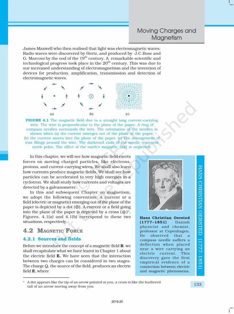
FIGURE 4.1 The magnetic field due to a straight long current-carrying

wire. The wire is perpendicular to the plane of the paper. A ring ofcompass needles surrounds the wire. The orientation of the needles is

shown when (a) the current emerges out of the plane of the paper,

(b) the current moves into the plane of the paper. (c) The arrangement ofiron filings around the wire. The darkened ends of the needle represent

north poles. The effect of the earth’s magnetic field is neglected.

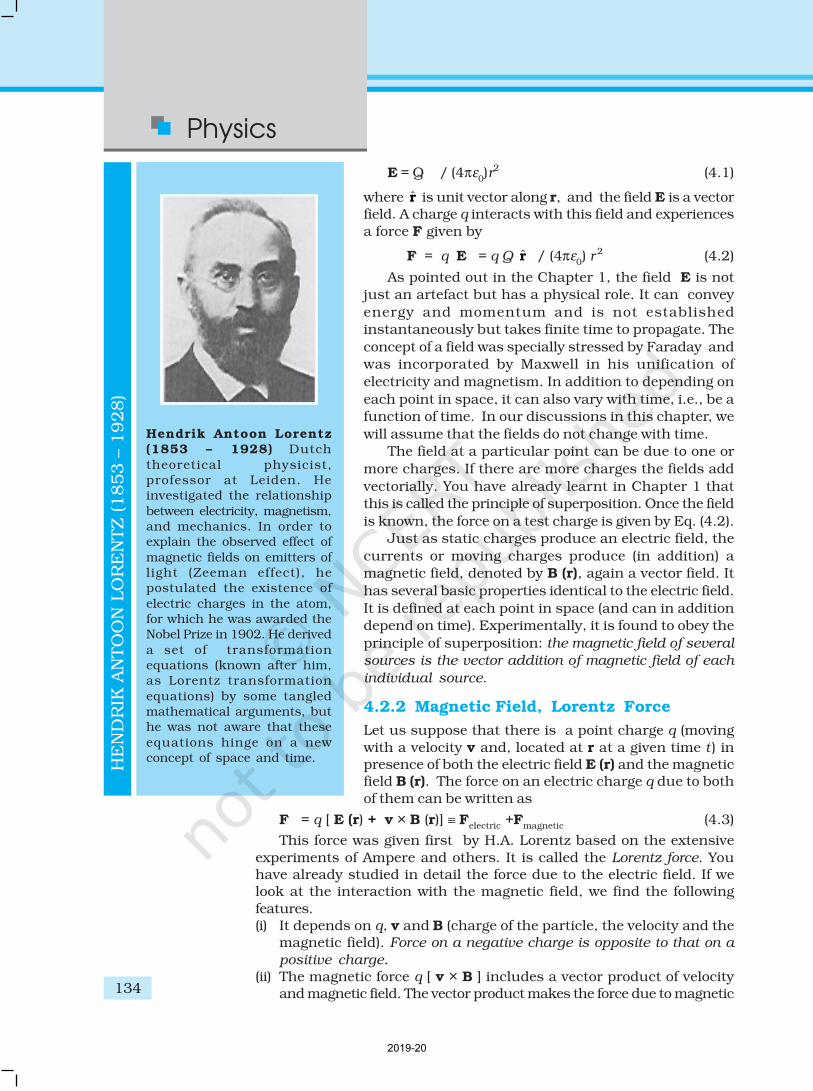
Hans Christian Oersted(1777–1851) Danish

physicist and chemist,professor at Copenhagen.He observed that a

compass needle suffers adeflection when placednear a wire carrying an

electric current. Thisdiscovery gave the firstempirical evidence of a

connection between electricand magnetic phenomena.

HA

NS

CH

RIS

TIA

N O

ER

STE

D (1

777–1851)

* A dot appears like the tip of an arrow pointed at you, a cross is like the feathered

tail of an arrow moving away from you.

2019-20

Physics

134

E = Q

r

/ (4πε0)r2 (4.1)

where r is unit vector along r, and the field E is a vectorfield. A charge q interacts with this field and experiences

a force F given by

F = q E = q Q r / (4πε0) r 2 (4.2)

As pointed out in the Chapter 1, the field E is not

just an artefact but has a physical role. It can convey

energy and momentum and is not established

instantaneously but takes finite time to propagate. The

concept of a field was specially stressed by Faraday and

was incorporated by Maxwell in his unification of

electricity and magnetism. In addition to depending on

each point in space, it can also vary with time, i.e., be a

function of time. In our discussions in this chapter, we

will assume that the fields do not change with time.

The field at a particular point can be due to one or

more charges. If there are more charges the fields add

vectorially. You have already learnt in Chapter 1 that

this is called the principle of superposition. Once the field

is known, the force on a test charge is given by Eq. (4.2).

Just as static charges produce an electric field, the

currents or moving charges produce (in addition) a

magnetic field, denoted by B (r), again a vector field. It

has several basic properties identical to the electric field.

It is defined at each point in space (and can in addition

depend on time). Experimentally, it is found to obey the

principle of superposition: the magnetic field of several

sources is the vector addition of magnetic field of each

individual source.

4.2.2 Magnetic Field, Lorentz Force

Let us suppose that there is a point charge q (moving

with a velocity v and, located at r at a given time t ) inpresence of both the electric field E (r) and the magneticfield B (r). The force on an electric charge q due to both

of them can be written as

F = q [ E (r) + v × B (r)] ≡ Felectric

+Fmagnetic

(4.3)

This force was given first by H.A. Lorentz based on the extensive

experiments of Ampere and others. It is called the Lorentz force. Youhave already studied in detail the force due to the electric field. If welook at the interaction with the magnetic field, we find the following

features.(i) It depends on q, v and B (charge of the particle, the velocity and the

magnetic field). Force on a negative charge is opposite to that on a

positive charge.

(ii) The magnetic force q [ v × B ] includes a vector product of velocityand magnetic field. The vector product makes the force due to magnetic

HE

ND

RIK

AN

TO

ON

LO

RE

NTZ (

1853 –

1928)

Hendrik Antoon Lorentz(1853 – 1928) Dutch

theoretical physicist,professor at Leiden. Heinvestigated the relationship

between electricity, magnetism,and mechanics. In order toexplain the observed effect of

magnetic fields on emitters oflight (Zeeman effect), hepostulated the existence of

electric charges in the atom,for which he was awarded theNobel Prize in 1902. He derived

a set of transformationequations (known after him,as Lorentz transformation

equations) by some tangledmathematical arguments, buthe was not aware that these

equations hinge on a newconcept of space and time.

2019-20

Moving Charges and

Magnetism

135

field vanish (become zero) if velocity and magnetic field are parallelor anti-parallel. The force acts in a (sideways) direction perpendicular

to both the velocity and the magnetic field.Its direction is given by the screw rule orright hand rule for vector (or cross) product

as illustrated in Fig. 4.2.(iii) The magnetic force is zero if charge is not

moving (as then |v|= 0). Only a moving

charge feels the magnetic force.The expression for the magnetic force helps

us to define the unit of the magnetic field, if

one takes q, F and v, all to be unity in the force

equation F = q [ v × B] =q v B sin θ n , where θis the angle between v and B [see Fig. 4.2 (a)].

The magnitude of magnetic field B is 1 SI unit,when the force acting on a unit charge (1 C),moving perpendicular to B with a speed 1m/s,

is one newton.Dimensionally, we have [B] = [F/qv] and the unitof B are Newton second / (coulomb metre). This

unit is called tesla (T) named after Nikola Tesla(1856 – 1943). Tesla is a rather large unit. A smaller unit (non-SI) calledgauss (=10–4 tesla) is also often used. The earth’s magnetic field is about

3.6 × 10–5 T. Table 4.1 lists magnetic fields over a wide range in theuniverse.

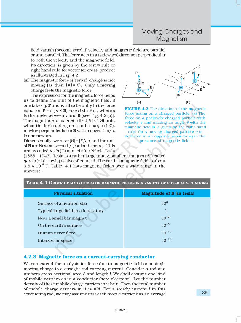
FIGURE 4.2 The direction of the magneticforce acting on a charged particle. (a) The

force on a positively charged particle withvelocity v and making an angle θ with themagnetic field B is given by the right-hand

rule. (b) A moving charged particle q isdeflected in an opposite sense to –q in the

presence of magnetic field.

TABLE 4.1 ORDER OF MAGNITUDES OF MAGNETIC FIELDS IN A VARIETY OF PHYSICAL SITUATIONS

Physical situation Magnitude of B (in tesla)

Surface of a neutron star 108

Typical large field in a laboratory 1

Near a small bar magnet 10–2

On the earth’s surface 10–5

Human nerve fibre 10–10

Interstellar space 10–12

4.2.3 Magnetic force on a current-carrying conductor

We can extend the analysis for force due to magnetic field on a singlemoving charge to a straight rod carrying current. Consider a rod of a

uniform cross-sectional area A and length l. We shall assume one kindof mobile carriers as in a conductor (here electrons). Let the numberdensity of these mobile charge carriers in it be n. Then the total number

of mobile charge carriers in it is nlA. For a steady current I in thisconducting rod, we may assume that each mobile carrier has an average

2019-20

Physics

136 EX

AM

PLE 4

.1

drift velocity vd (see Chapter 3). In the presence of an external magnetic

field B, the force on these carriers is:

F = (nlA)q vd ××××× B

where q is the value of the charge on a carrier. Now nq vd is the current

density j and |(nq vd)|A is the current I (see Chapter 3 for the discussion

of current and current density). Thus,

F = [(nq vd )lA] × B = [ jAl ] ××××× B

= Il ××××× B (4.4)

where l is a vector of magnitude l, the length of the rod, and with a directionidentical to the current I. Note that the current I is not a vector. In the laststep leading to Eq. (4.4), we have transferred the vector sign from j to l.

Equation (4.4) holds for a straight rod. In this equation, B is the externalmagnetic field. It is not the field produced by the current-carrying rod. Ifthe wire has an arbitrary shape we can calculate the Lorentz force on it

by considering it as a collection of linear strips dlj and summing

jj

Id ×= ∑F Bl

This summation can be converted to an integral in most cases.

ON PERMITTIVITY AND PERMEABILITY

In the universal law of gravitation, we say that any two point masses exert a force oneach other which is proportional to the product of the masses m

1, m

2 and inversely

proportional to the square of the distance r between them. We write it as F = Gm1m

2/r2

where G is the universal constant of gravitation. Similarly, in Coulomb’s law of electrostaticswe write the force between two point charges q

1, q

2, separated by a distance r as

F = kq1q

2/r 2 where k is a constant of proportionality. In SI units, k is taken as

1/4πε where ε is the permittivity of the medium. Also in magnetism, we get anotherconstant, which in SI units, is taken as µ/4π where µ is the permeability of the medium.

Although G, ε and µ arise as proportionality constants, there is a difference betweengravitational force and electromagnetic force. While the gravitational force does not dependon the intervening medium, the electromagnetic force depends on the medium between

the two charges or magnets. Hence, while G is a universal constant, ε and µ depend onthe medium. They have different values for different media. The product εµ turns out tobe related to the speed v of electromagnetic radiation in the medium through εµ =1/ v 2.

Electric permittivity ε is a physical quantity that describes how an electric field affectsand is affected by a medium. It is determined by the ability of a material to polarise inresponse to an applied field, and thereby to cancel, partially, the field inside the material.

Similarly, magnetic permeability µ is the ability of a substance to acquire magnetisation inmagnetic fields. It is a measure of the extent to which magnetic field can penetrate matter.

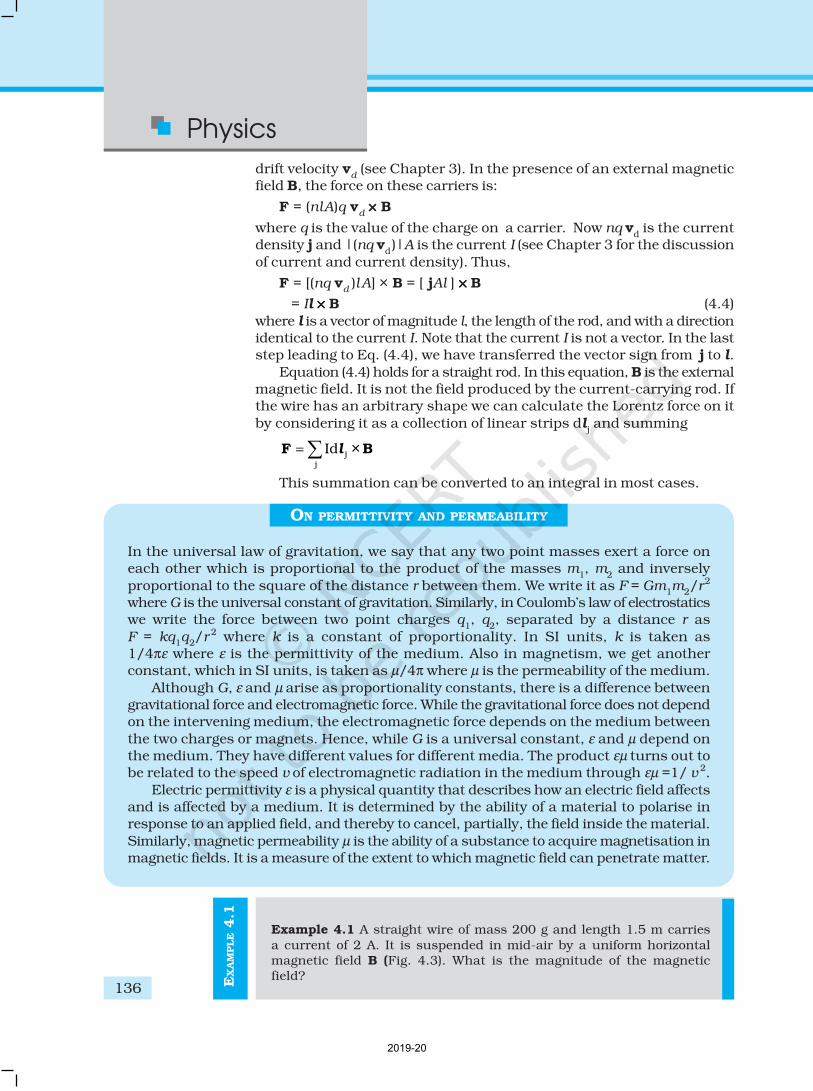
Example 4.1 A straight wire of mass 200 g and length 1.5 m carries

a current of 2 A. It is suspended in mid-air by a uniform horizontalmagnetic field B (Fig. 4.3). What is the magnitude of the magneticfield?

2019-20

Moving Charges and

Magnetism

137

EX

AM

PLE 4

.1

FIGURE 4.3

Solution From Eq. (4.4), we find that there is an upward force F, ofmagnitude IlB,. For mid-air suspension, this must be balanced bythe force due to gravity:

m g = I lB

m g

BI l

=

0.2 9.8

0.65 T2 1.5

×= =

×

Note that it would have been sufficient to specify m/l, the mass per

unit length of the wire. The earth’s magnetic field is approximately4 × 10–5 T and we have ignored it.

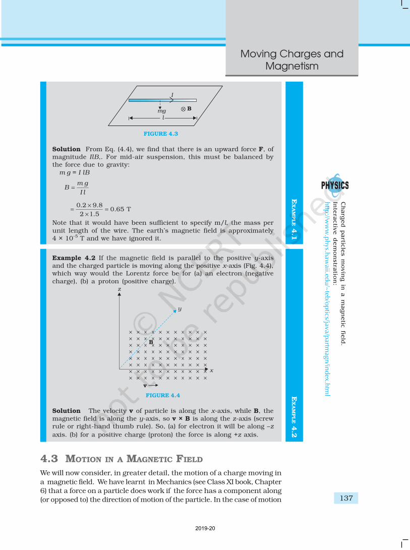
Example 4.2 If the magnetic field is parallel to the positive y-axisand the charged particle is moving along the positive x-axis (Fig. 4.4),which way would the Lorentz force be for (a) an electron (negative

charge), (b) a proton (positive charge).

FIGURE 4.4

Solution The velocity v of particle is along the x-axis, while B, themagnetic field is along the y-axis, so v × B is along the z-axis (screwrule or right-hand thumb rule). So, (a) for electron it will be along –z

axis. (b) for a positive charge (proton) the force is along +z axis.

4.3 MOTION IN A MAGNETIC FIELD

We will now consider, in greater detail, the motion of a charge moving in

a magnetic field. We have learnt in Mechanics (see Class XI book, Chapter

6) that a force on a particle does work if the force has a component along

(or opposed to) the direction of motion of the particle. In the case of motion

EX

AM

PLE 4

.2

Ch

arg

ed

p

artic

les m

ovin

g in

a m

ag

netic

fie

ld.

Inte

ractiv

e d

em

on

stra

tion

:

http

://ww

w.p

hys.h

awaii.ed

u/~

teb/o

ptics/java/p

artmagn

/index.h

tml

2019-20

Physics

138

of a charge in a magnetic field, the magnetic force isperpendicular to the velocity of the particle. So no work is done

and no change in the magnitude of the velocity is produced(though the direction of momentum may be changed). [Noticethat this is unlike the force due to an electric field, qE, which

can have a component parallel (or antiparallel) to motion andthus can transfer energy in addition to momentum.]

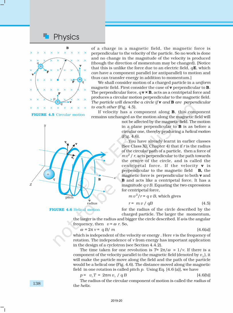
We shall consider motion of a charged particle in a uniform

magnetic field. First consider the case of v perpendicular to B.The perpendicular force, q v × B, acts as a centripetal force andproduces a circular motion perpendicular to the magnetic field.

The particle will describe a circle if v and B are perpendicular

to each other (Fig. 4.5).If velocity has a component along B, this component

remains unchanged as the motion along the magnetic field willnot be affected by the magnetic field. The motionin a plane perpendicular to B is as before a

circular one, thereby producing a helical motion

(Fig. 4.6).You have already learnt in earlier classes

(See Class XI, Chapter 4) that if r is the radiusof the circular path of a particle, then a force ofm v2 / r, acts perpendicular to the path towards

the centre of the circle, and is called thecentripetal force. If the velocity v isperpendicular to the magnetic field B, the

magnetic force is perpendicular to both v andB and acts like a centripetal force. It has amagnitude q v B. Equating the two expressions

for centripetal force,

m v 2/r = q v B, which gives

r = m v / qB (4.5)

for the radius of the circle described by thecharged particle. The larger the momentum,

the larger is the radius and bigger the circle described. If ω is the angular

frequency, then v = ω r. So,

ω = 2π ν = q B/ m [4.6(a)]

which is independent of the velocity or energy . Here ν is the frequency ofrotation. The independence of ν from energy has important application

in the design of a cyclotron (see Section 4.4.2).The time taken for one revolution is T= 2π/ω ≡ 1/ν. If there is a

component of the velocity parallel to the magnetic field (denoted by v||), it

will make the particle move along the field and the path of the particlewould be a helical one (Fig. 4.6). The distance moved along the magneticfield in one rotation is called pitch p. Using Eq. [4.6 (a)], we have

p = v||T = 2πm v

|| / q B [4.6(b)]

The radius of the circular component of motion is called the radius ofthe helix.

FIGURE 4.5 Circular motion

FIGURE 4.6 Helical motion

2019-20

Moving Charges and

Magnetism

139

EX

AM

PLE 4

.3

Example 4.3 What is the radius of the path of an electron (mass

9 × 10-31 kg and charge 1.6 × 10–19 C) moving at a speed of 3 ×107 m/s ina magnetic field of 6 × 10–4 T perpendicular to it? What is itsfrequency? Calculate its energy in keV. ( 1 eV = 1.6 × 10–19 J).

Solution Using Eq. (4.5) we findr = m v / (qB ) = 9 ×10–31 kg × 3 × 107 m s–1 / ( 1.6 × 10–19 C × 6 × 10–4 T ) = 26 × 10–2 m = 26 cm

ν = v / (2 πr) = 2×106 s–1 = 2×106 Hz =2 MHz.E = (½ )mv 2 = (½ ) 9 × 10–31 kg × 9 × 1014 m2/s2 = 40.5 ×10–17 J

≈ 4×10–16 J = 2.5 keV.

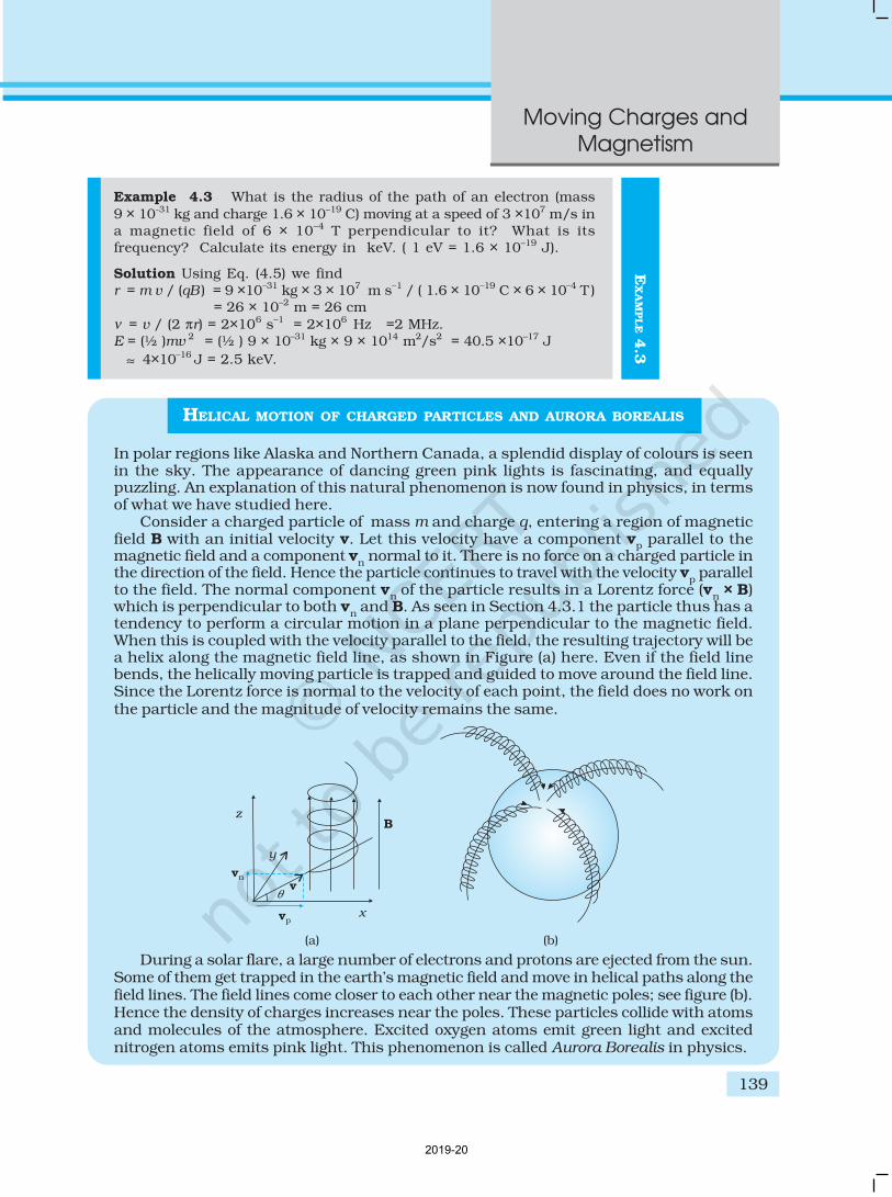
HELICAL MOTION OF CHARGED PARTICLES AND AURORA BOREALIS

In polar regions like Alaska and Northern Canada, a splendid display of colours is seenin the sky. The appearance of dancing green pink lights is fascinating, and equallypuzzling. An explanation of this natural phenomenon is now found in physics, in termsof what we have studied here.

Consider a charged particle of mass m and charge q, entering a region of magneticfield B with an initial velocity v. Let this velocity have a component v

p parallel to the

magnetic field and a component vn normal to it. There is no force on a charged particle in

the direction of the field. Hence the particle continues to travel with the velocity vp parallel

to the field. The normal component vn of the particle results in a Lorentz force (v

n × B)

which is perpendicular to both vn and B. As seen in Section 4.3.1 the particle thus has a

tendency to perform a circular motion in a plane perpendicular to the magnetic field.When this is coupled with the velocity parallel to the field, the resulting trajectory will bea helix along the magnetic field line, as shown in Figure (a) here. Even if the field linebends, the helically moving particle is trapped and guided to move around the field line.Since the Lorentz force is normal to the velocity of each point, the field does no work onthe particle and the magnitude of velocity remains the same.

During a solar flare, a large number of electrons and protons are ejected from the sun.Some of them get trapped in the earth’s magnetic field and move in helical paths along thefield lines. The field lines come closer to each other near the magnetic poles; see figure (b).Hence the density of charges increases near the poles. These particles collide with atomsand molecules of the atmosphere. Excited oxygen atoms emit green light and excitednitrogen atoms emits pink light. This phenomenon is called Aurora Borealis in physics.

2019-20

Physics

140

4.4 MOTION IN COMBINED ELECTRIC AND MAGNETIC

FIELDS

4.4.1 Velocity selector

You know that a charge q moving with velocity v in presence of bothelectric and magnetic fields experiences a force given by Eq. (4.3), that is,

F = q (E + v × B) = FE + F

B

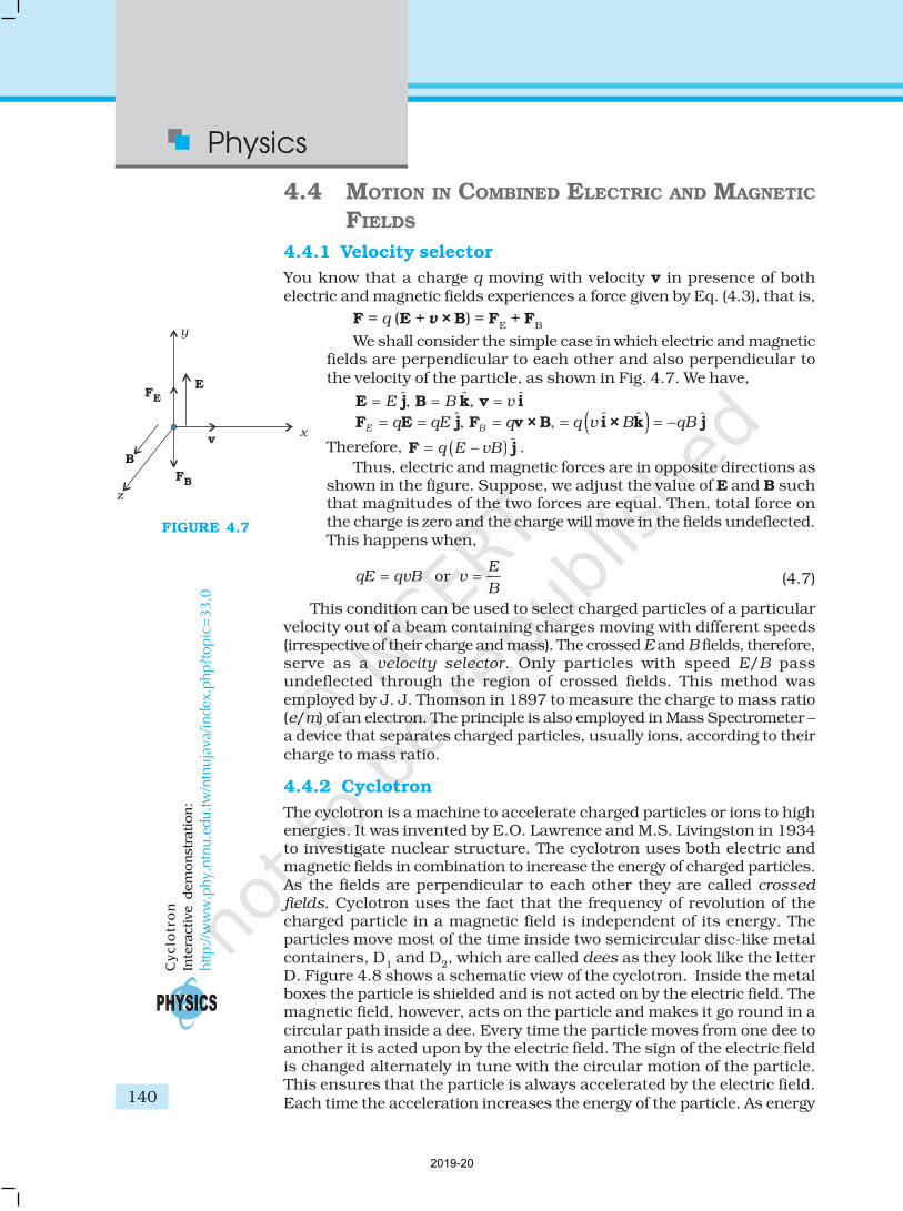
We shall consider the simple case in which electric and magneticfields are perpendicular to each other and also perpendicular tothe velocity of the particle, as shown in Fig. 4.7. We have,

ˆ ˆ ˆ, ,= = =E j B k v iE B v

( )ˆ ˆ ˆ ˆ, , –E Bq qE q q v B qB= = = = =F E j F v × B i × k j

Therefore, ( ) ˆ–q E vB=F j .

Thus, electric and magnetic forces are in opposite directions asshown in the figure. Suppose, we adjust the value of E and B suchthat magnitudes of the two forces are equal. Then, total force onthe charge is zero and the charge will move in the fields undeflected.This happens when,

orE

qE qvB vB

= = (4.7)

This condition can be used to select charged particles of a particularvelocity out of a beam containing charges moving with different speeds(irrespective of their charge and mass). The crossed E and B fields, therefore,serve as a velocity selector. Only particles with speed E/B passundeflected through the region of crossed fields. This method wasemployed by J. J. Thomson in 1897 to measure the charge to mass ratio(e/m) of an electron. The principle is also employed in Mass Spectrometer –a device that separates charged particles, usually ions, according to theircharge to mass ratio.

4.4.2 Cyclotron

The cyclotron is a machine to accelerate charged particles or ions to highenergies. It was invented by E.O. Lawrence and M.S. Livingston in 1934to investigate nuclear structure. The cyclotron uses both electric andmagnetic fields in combination to increase the energy of charged particles.As the fields are perpendicular to each other they are called crossedfields. Cyclotron uses the fact that the frequency of revolution of thecharged particle in a magnetic field is independent of its energy. Theparticles move most of the time inside two semicircular disc-like metalcontainers, D

1 and D

2, which are called dees as they look like the letter

D. Figure 4.8 shows a schematic view of the cyclotron. Inside the metalboxes the particle is shielded and is not acted on by the electric field. Themagnetic field, however, acts on the particle and makes it go round in acircular path inside a dee. Every time the particle moves from one dee toanother it is acted upon by the electric field. The sign of the electric fieldis changed alternately in tune with the circular motion of the particle.This ensures that the particle is always accelerated by the electric field.Each time the acceleration increases the energy of the particle. As energy

FIGURE 4.7

Cyclo

tro

n

Inte

racti

ve d

em

on

str

ati

on

:

http://w

ww

.phy.

ntn

u.e

du.tw

/ntn

uja

va/index

.php?t

opic

=33.0

2019-20

Moving Charges and

Magnetism

141

increases, the radius of the circular path increases. So the path is aspiral one.

The whole assembly is evacuated to minimise collisions between theions and the air molecules. A high frequency alternating voltage is appliedto the dees. In the sketch shown in Fig. 4.8, positive ions or positively

charged particles (e.g., protons) are released at the centre P. They movein a semi-circular path in one of the dees and arrive in the gap betweenthe dees in a time interval T/2; where T, the period of revolution, is given

by Eq. (4.6),

1 2

c

mT

qBν

π= =

or 2

c

qB

mν =

π(4.8)

This frequency is called the cyclotron frequency for obvious reasonsand is denoted by ν

c .

The frequency νa of the applied voltage is adjusted so that the polarity

of the dees is reversed in the same time that it takes the ions to complete

one half of the revolution. The requirement νa = ν

c is called the resonance

condition. The phase of the supply is adjusted so that when the positive

ions arrive at the edge of D1, D

2 is at a lower

potential and the ions are accelerated across the

gap. Inside the dees the particles travel in a region

free of the electric field. The increase in their

kinetic energy is qV each time they cross from

one dee to another (V refers to the voltage across

the dees at that time). From Eq. (4.5), it is clear

that the radius of their path goes on increasing

each time their kinetic energy increases. The ions

are repeatedly accelerated across the dees until

they have the required energy to have a radius

approximately that of the dees. They are then

deflected by a magnetic field and leave the system

via an exit slit. From Eq. (4.5) we have,

qBRv

m= (4.9)

where R is the radius of the trajectory at exit, and

equals the radius of a dee.Hence, the kinetic energy of the ions is,

2 2 221

2 2

q B Rm

m=v (4.10)

The operation of the cyclotron is based on thefact that the time for one revolution of an ion isindependent of its speed or radius of its orbit.

The cyclotron is used to bombard nuclei withenergetic particles, so accelerated by it, and study

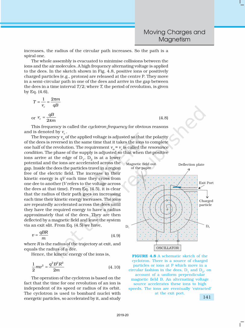
FIGURE 4.8 A schematic sketch of the

cyclotron. There is a source of chargedparticles or ions at P which move in a

circular fashion in the dees, D1 and D

2, on

account of a uniform perpendicularmagnetic field B. An alternating voltagesource accelerates these ions to high

speeds. The ions are eventually ‘extracted’at the exit port.

2019-20

Physics

142

EX

AM

PLE 4

.4

the resulting nuclear reactions. It is also used to implant ions into solidsand modify their properties or even synthesise new materials. It is used

in hospitals to produce radioactive substances which can be used indiagnosis and treatment.

Example 4.4 A cyclotron’s oscillator frequency is 10 MHz. What

should be the operating magnetic field for accelerating protons? Ifthe radius of its ‘dees’ is 60 cm, what is the kinetic energy (in MeV) ofthe proton beam produced by the accelerator.

(e =1.60 × 10–19 C, mp = 1.67 × 10–27 kg, 1 MeV = 1.6 × 10–13 J).

Solution The oscillator frequency should be same as proton’scyclotron frequency.Using Eqs. (4.5) and [4.6(a)] we have

B = 2π m ν/q =6.3 ×1.67 × 10–27 × 107 / (1.6 × 10–19) = 0.66 T

Final velocity of protons is

v = r × 2π ν = 0.6 m × 6.3 ×107 = 3.78 × 107 m/s.

E = ½ mv 2 = 1.67 ×10–27 × 14.3 × 1014 / (2 × 1.6 × 10–13) = 7 MeV.

ACCELERATORS IN INDIA

India has been an early entrant in the area of accelerator-based research. The vision ofDr. Meghnath Saha created a 37" Cyclotron in the Saha Institute of Nuclear Physics inKolkata in 1953. This was soon followed by a series of Cockroft-Walton type of acceleratorsestablished in Tata Institute of Fundamental Research (TIFR), Mumbai, Aligarh MuslimUniversity (AMU), Aligarh, Bose Institute, Kolkata and Andhra University, Waltair.

The sixties saw the commissioning of a number of Van de Graaff accelerators: a 5.5 MVterminal machine in Bhabha Atomic Research Centre (BARC), Mumbai (1963); a 2 MV terminalmachine in Indian Institute of Technology (IIT), Kanpur; a 400 kV terminal machine in BanarasHindu University (BHU), Varanasi; and Punjabi University, Patiala. One 66 cm Cyclotrondonated by the Rochester University of USA was commissioned in Panjab University,Chandigarh. A small electron accelerator was also established in University of Pune, Pune.

In a major initiative taken in the seventies and eighties, a Variable Energy Cyclotron wasbuilt indigenously in Variable Energy Cyclotron Centre (VECC), Kolkata; 2 MV Tandem Vande Graaff accelerator was developed and built in BARC and a 14 MV Tandem Pelletronaccelerator was installed in TIFR.

This was soon followed by a 15 MV Tandem Pelletron established by University GrantsCommission (UGC), as an inter-university facility in Inter-University Accelerator Centre(IUAC), New Delhi; a 3 MV Tandem Pelletron in Institute of Physics, Bhubaneswar; and two1.7 MV Tandetrons in Atomic Minerals Directorate for Exploration and Research, Hyderabadand Indira Gandhi Centre for Atomic Research, Kalpakkam. Both TIFR and IUAC areaugmenting their facilities with the addition of superconducting LINAC modules to acceleratethe ions to higher energies.

Besides these ion accelerators, the Department of Atomic Energy (DAE) has developedmany electron accelerators. A 2 GeV Synchrotron Radiation Source is being built in RajaRamanna Centre for Advanced Technologies, Indore.

The Department of Atomic Energy is considering Accelerator Driven Systems (ADS) forpower production and fissile material breeding as future options.

2019-20

Moving Charges and

Magnetism

143

4.5 MAGNETIC FIELD DUE TO A CURRENT ELEMENT,BIOT-SAVART LAW

All magnetic fields that we know are due to currents (or moving charges)

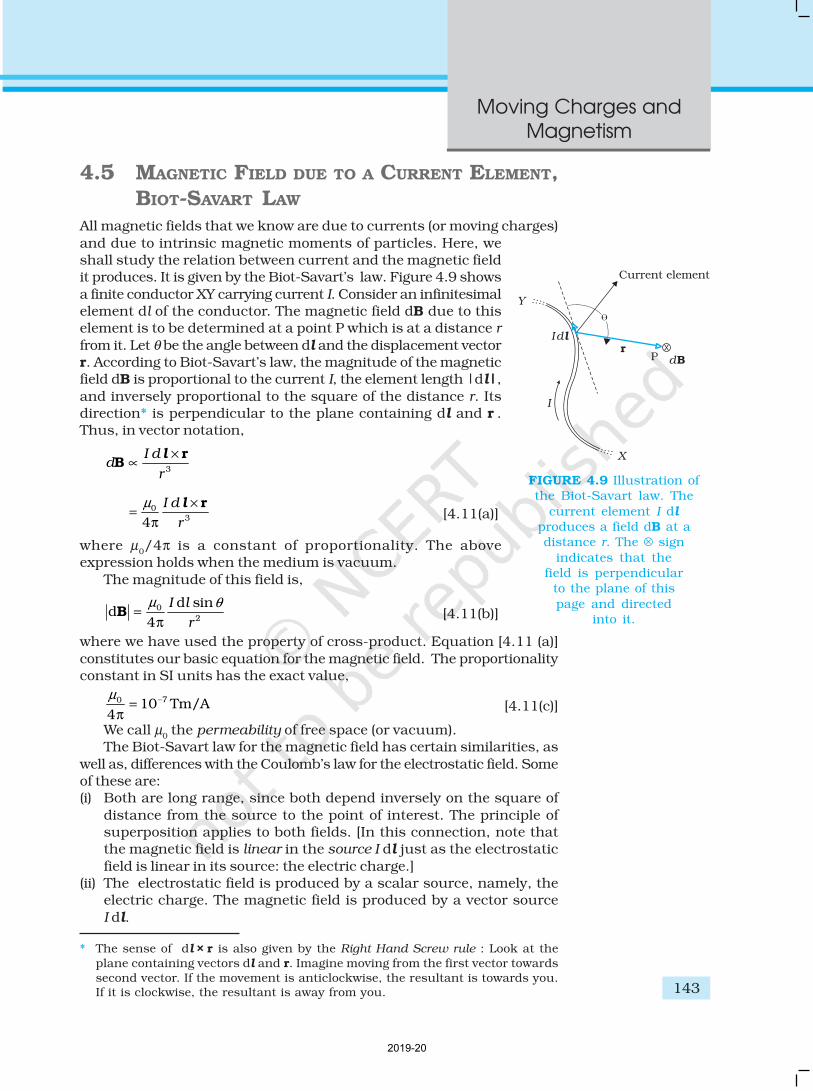
and due to intrinsic magnetic moments of particles. Here, weshall study the relation between current and the magnetic fieldit produces. It is given by the Biot-Savart’s law. Figure 4.9 shows

a finite conductor XY carrying current I. Consider an infinitesimalelement dl of the conductor. The magnetic field dB due to thiselement is to be determined at a point P which is at a distance r

from it. Let θ be the angle between dl and the displacement vectorr. According to Biot-Savart’s law, the magnitude of the magneticfield dB is proportional to the current I, the element length |dl|,

and inversely proportional to the square of the distance r. Itsdirection* is perpendicular to the plane containing dl and r .Thus, in vector notation,

3

I dd

r

×∝

rB

l

0

34

I d

r

µ ×=

π

rl [4.11(a)]

where µ0/4π is a constant of proportionality. The above

expression holds when the medium is vacuum.

The magnitude of this field is,

0

2

d sind

4

I l

r

µ θ=

πB [4.11(b)]

where we have used the property of cross-product. Equation [4.11 (a)]

constitutes our basic equation for the magnetic field. The proportionalityconstant in SI units has the exact value,

70 10 Tm/A4

µ −=π

[4.11(c)]

We call µ0 the permeability of free space (or vacuum).

The Biot-Savart law for the magnetic field has certain similarities, as

well as, differences with the Coulomb’s law for the electrostatic field. Someof these are:(i) Both are long range, since both depend inversely on the square of

distance from the source to the point of interest. The principle ofsuperposition applies to both fields. [In this connection, note thatthe magnetic field is linear in the source I dl just as the electrostatic

field is linear in its source: the electric charge.](ii) The electrostatic field is produced by a scalar source, namely, the

electric charge. The magnetic field is produced by a vector source

I dl.

* The sense of dl × r is also given by the Right Hand Screw rule : Look at the

plane containing vectors dl and r. Imagine moving from the first vector towards

second vector. If the movement is anticlockwise, the resultant is towards you.If it is clockwise, the resultant is away from you.

FIGURE 4.9 Illustration ofthe Biot-Savart law. The

current element I dl

produces a field dB at adistance r. The ⊗ sign

indicates that thefield is perpendicular

to the plane of this

page and directedinto it.

2019-20

Physics

144 EX

AM

PLE 4

.5

(iii) The electrostatic field is along the displacement vector joining thesource and the field point. The magnetic field is perpendicular to the

plane containing the displacement vector r and the current elementI dl.

(iv) There is an angle dependence in the Biot-Savart law which is not

present in the electrostatic case. In Fig. 4.9, the magnetic field at anypoint in the direction of dl (the dashed line) is zero. Along this line,θ = 0, sin θ = 0 and from Eq. [4.11(a)], |dB| = 0.

There is an interesting relation between ε0, the permittivity of free

space; µ0, the permeability of free space; and c, the speed of light in

vacuum:

( ) 00 0 04

4

µε µ ε

= π

π ( )7

9

110

9 10

− =

×8 2 2

1 1

(3 10 ) c= =

×

We will discuss this connection further in Chapter 8 on the

electromagnetic waves. Since the speed of light in vacuum is constant,the product µ

0ε

0 is fixed in magnitude. Choosing the value of either ε

0 or

µ0, fixes the value of the other. In SI units, µ

0 is fixed to be equal to

4π × 10–7 in magnitude.

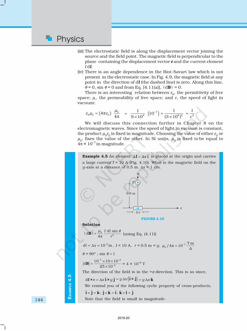
Example 4.5 An element ˆ∆ = ∆x il is placed at the origin and carries

a large current I = 10 A (Fig. 4.10). What is the magnetic field on they-axis at a distance of 0.5 m. ∆x = 1 cm.

FIGURE 4.10

Solution

0

2

d sin|d |

4

I l

r

µ θ=

πB [using Eq. (4.11)]

2d 10 ml x −= ∆ = , I = 10 A, r = 0.5 m = y, 7

0

T m/4 10

Aµ −π =

θ = 90° ; sin θ = 1

7 2

2

10 10 10d

25 10

− −

−

× ×=

×B = 4 × 10–8 T

The direction of the field is in the +z-direction. This is so since,

ˆ ˆd = ∆× i × jx yrl ( )ˆ ˆy x= ∆ i × j ˆy x= ∆ k

We remind you of the following cyclic property of cross-products,

ˆ ˆ ˆ ˆ ˆ ˆ ˆ ˆ ˆ; ;× = × = × =i j k j k i k i j

Note that the field is small in magnitude.

2019-20

Moving Charges and

Magnetism

145

In the next section, we shall use the Biot-Savart law to calculate themagnetic field due to a circular loop.

4.6 MAGNETIC FIELD ON THE AXIS OF A CIRCULAR

CURRENT LOOP

In this section, we shall evaluate the magnetic field due to a circular coilalong its axis. The evaluation entails summing up the effect of infinitesimalcurrent elements (I dl) mentioned in the previous section.

We assume that the current I is steady and that theevaluation is carried out in free space (i.e., vacuum).

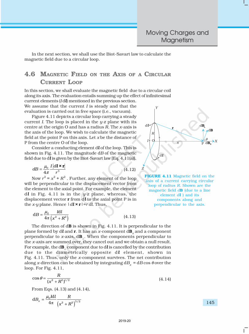
Figure 4.11 depicts a circular loop carrying a steady

current I. The loop is placed in the y-z plane with itscentre at the origin O and has a radius R. The x-axis isthe axis of the loop. We wish to calculate the magnetic

field at the point P on this axis. Let x be the distance ofP from the centre O of the loop.

Consider a conducting element dl of the loop. This is

shown in Fig. 4.11. The magnitude dB of the magneticfield due to dl is given by the Biot-Savart law [Eq. 4.11(a)],

0

34=

× rI ddB

r

µ

π

l(4.12)

Now r2 = x2 + R2 . Further, any element of the loopwill be perpendicular to the displacement vector fromthe element to the axial point. For example, the element

dl in Fig. 4.11 is in the y-z plane, whereas, thedisplacement vector r from dl to the axial point P is inthe x-y plane. Hence |dl × r|=r dl. Thus,

( )π

0

2 2

dd

4

I lB

x R

µ=

+ (4.13)

The direction of dB is shown in Fig. 4.11. It is perpendicular to the

plane formed by dl and r. It has an x-component dBx and a component

perpendicular to x-axis, dB⊥. When the components perpendicular to

the x-axis are summed over, they cancel out and we obtain a null result.

For example, the dB⊥ component due to dl is cancelled by the contribution

due to the diametrically opposite dl element, shown inFig. 4.11. Thus, only the x-component survives. The net contribution

along x-direction can be obtained by integrating dBx = dB cos θ over the

loop. For Fig. 4.11,

2 2 1/2cos

( )

R

x Rθ =

+ (4.14)

From Eqs. (4.13) and (4.14),

( )π

0

3/22 2

dd

4x

I l RB

x R

µ=

+

FIGURE 4.11 Magnetic field on theaxis of a current carrying circular

loop of radius R. Shown are the

magnetic field dB (due to a lineelement dl ) and its

components along and

perpendicular to the axis.

2019-20

Physics

146 EX

AM

PLE 4

.6

The summation of elements dl over the loop yields 2πR, thecircumference of the loop. Thus, the magnetic field at P due to entire

circular loop is

( )

20

3/22 2

ˆ ˆ

2x

I RB

x R

µ= =

+B i i (4.15)

As a special case of the above result, we may obtain the field at the centreof the loop. Here x = 0, and we obtain,

00

ˆ2

I

R

µ=B i (4.16)

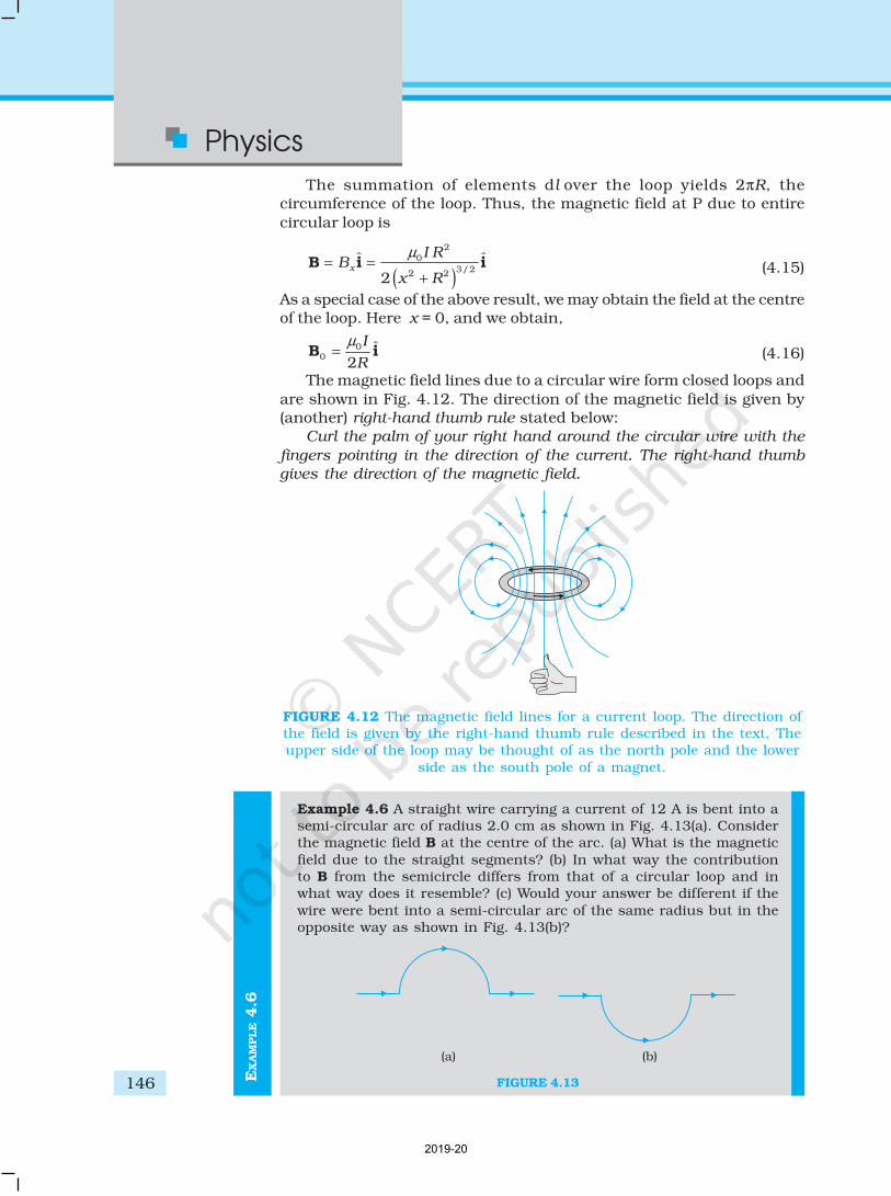
The magnetic field lines due to a circular wire form closed loops and

are shown in Fig. 4.12. The direction of the magnetic field is given by(another) right-hand thumb rule stated below:

Curl the palm of your right hand around the circular wire with the

fingers pointing in the direction of the current. The right-hand thumb

gives the direction of the magnetic field.

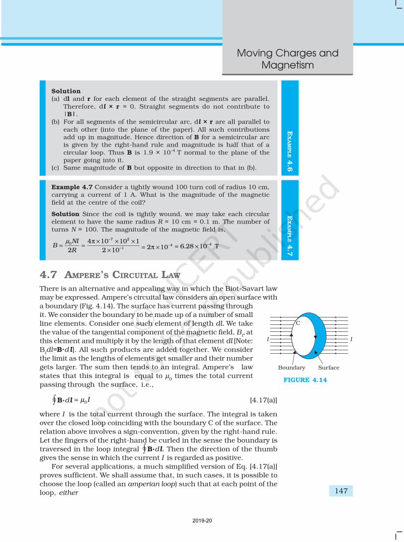
Example 4.6 A straight wire carrying a current of 12 A is bent into asemi-circular arc of radius 2.0 cm as shown in Fig. 4.13(a). Considerthe magnetic field B at the centre of the arc. (a) What is the magnetic

field due to the straight segments? (b) In what way the contributionto B from the semicircle differs from that of a circular loop and inwhat way does it resemble? (c) Would your answer be different if the

wire were bent into a semi-circular arc of the same radius but in theopposite way as shown in Fig. 4.13(b)?

FIGURE 4.13

FIGURE 4.12 The magnetic field lines for a current loop. The direction ofthe field is given by the right-hand thumb rule described in the text. Theupper side of the loop may be thought of as the north pole and the lower

side as the south pole of a magnet.

2019-20

Moving Charges and

Magnetism

147

EX

AM

PLE 4

.6

Solution(a) dl and r for each element of the straight segments are parallel.

Therefore, dl × r = 0. Straight segments do not contribute to|B|.

(b) For all segments of the semicircular arc, dl × r are all parallel to

each other (into the plane of the paper). All such contributionsadd up in magnitude. Hence direction of B for a semicircular arcis given by the right-hand rule and magnitude is half that of a

circular loop. Thus B is 1.9 × 10–4 T normal to the plane of thepaper going into it.

(c) Same magnitude of B but opposite in direction to that in (b).

Example 4.7 Consider a tightly wound 100 turn coil of radius 10 cm,carrying a current of 1 A. What is the magnitude of the magnetic

field at the centre of the coil?

Solution Since the coil is tightly wound, we may take each circularelement to have the same radius R = 10 cm = 0.1 m. The number of

turns N = 100. The magnitude of the magnetic field is,

–7 20

–1

4 10 10 1

2 2 10

NIB

R

µ π × × ×= =

×42 10−

= π ×46 28 10 T. −= ×

4.7 AMPERE’S CIRCUITAL LAW

There is an alternative and appealing way in which the Biot-Savart law

may be expressed. Ampere’s circuital law considers an open surface with

a boundary (Fig. 4.14). The surface has current passing through

it. We consider the boundary to be made up of a number of small

line elements. Consider one such element of length dl. We take

the value of the tangential component of the magnetic field, Bt, at

this element and multiply it by the length of that element dl [Note:

Btdl=B.d l]. All such products are added together. We consider

the limit as the lengths of elements get smaller and their number

gets larger. The sum then tends to an integral. Ampere’s law

states that this integral is equal to µ0 times the total current

passing through the surface, i.e.,

“B.dl.d Il = µ0 [4.17(a)]

where I is the total current through the surface. The integral is taken

over the closed loop coinciding with the boundary C of the surface. The

relation above involves a sign-convention, given by the right-hand rule.

Let the fingers of the right-hand be curled in the sense the boundary is

traversed in the loop integral “B.dl. Then the direction of the thumb

gives the sense in which the current I is regarded as positive.

For several applications, a much simplified version of Eq. [4.17(a)]

proves sufficient. We shall assume that, in such cases, it is possible to

choose the loop (called an amperian loop) such that at each point of the

loop, either

FIGURE 4.14

EX

AM

PLE 4

.7

2019-20

Physics

148

(i) B is tangential to the loop and is a non-zero constant

B, or

(ii) B is normal to the loop, or

(iii) B vanishes.Now, let L be the length (part) of the loop for which B

is tangential. Let Ie be the current enclosed by the loop.

Then, Eq. (4.17) reduces to,

BL =µ0Ie

[4.17(b)]

When there is a system with a symmetry such as for

a straight infinite current-carrying wire in Fig. 4.15, theAmpere’s law enables an easy evaluation of the magneticfield, much the same way Gauss’ law helps in

determination of the electric field. This is exhibited in theExample 4.9 below. The boundary of the loop chosen isa circle and magnetic field is tangential to the

circumference of the circle. The law gives, for the left handside of Eq. [4.17 (b)], B. 2πr. We find that the magneticfield at a distance r outside the wire is tangential and

given by

B × 2πr = µ0 I,

B = µ0 I/ (2πr) (4.18)

The above result for the infinite wire is interestingfrom several points of view.

(i) It implies that the field at every point on a circle ofradius r, (with the wire along the axis), is same inmagnitude. In other words, the magnetic field

possesses what is called a cylindrical symmetry. Thefield that normally can depend on three coordinatesdepends only on one: r. Whenever there is symmetry,

the solutions simplify.(ii) The field direction at any point on this circle is

tangential to it. Thus, the lines of constant magnitude

of magnetic field form concentric circles. Notice now,

in Fig. 4.1(c), the iron filings form concentric circles.These lines called magnetic field lines form closed

loops. This is unlike the electrostatic field lines which

originate from positive charges and end at negative

charges. The expression for the magnetic field of astraight wire provides a theoretical justification to

Oersted’s experiments.

(iii) Another interesting point to note is that even though

the wire is infinite, the field due to it at a non-zerodistance is not infinite. It tends to blow up only when

we come very close to the wire. The field is directly

proportional to the current and inversely proportional

to the distance from the (infinitely long) currentsource.

AN

DR

E A

MPE

RE

(1775 –

1836)

Andre Ampere (1775 –

1836) Andre Marie Amperewas a French physicist,mathematician and chemist

who founded the science ofelectrodynamics. Amperewas a child prodigy

who mastered advancedmathematics by the age of12. Ampere grasped the

significance of Oersted’sdiscovery. He carried out alarge series of experiments

to explore the relationshipbetween current electricityand magnetism. These

investigations culminatedin 1827 with thepublication of the

‘Mathematical Theory ofElectrodynamic Pheno-mena Deduced Solely from

Experiments’. He hypo-thesised that all magneticphenomena are due to

circulating electriccurrents. Ampere washumble and absent-

minded. He once forgot aninvitation to dine with theEmperor Napoleon. He died

of pneumonia at the age of61. His gravestone bearsthe epitaph: Tandem Felix

(Happy at last).

2019-20

Moving Charges and

Magnetism

149

EX

AM

PLE 4

.8

(iv) There exists a simple rule to determine the direction of the magneticfield due to a long wire. This rule, called the right-hand rule*, is:

Grasp the wire in your right hand with your extended thumb pointing

in the direction of the current. Your fingers will curl around in the

direction of the magnetic field.

Ampere’s circuital law is not new in content from Biot-Savart law.Both relate the magnetic field and the current, and both express the samephysical consequences of a steady electrical current. Ampere’s law is to

Biot-Savart law, what Gauss’s law is to Coulomb’s law. Both, Ampere’sand Gauss’s law relate a physical quantity on the periphery or boundary(magnetic or electric field) to another physical quantity, namely, the source,

in the interior (current or charge). We also note that Ampere’s circuitallaw holds for steady currents which do not fluctuate with time. Thefollowing example will help us understand what is meant by the term

enclosed current.

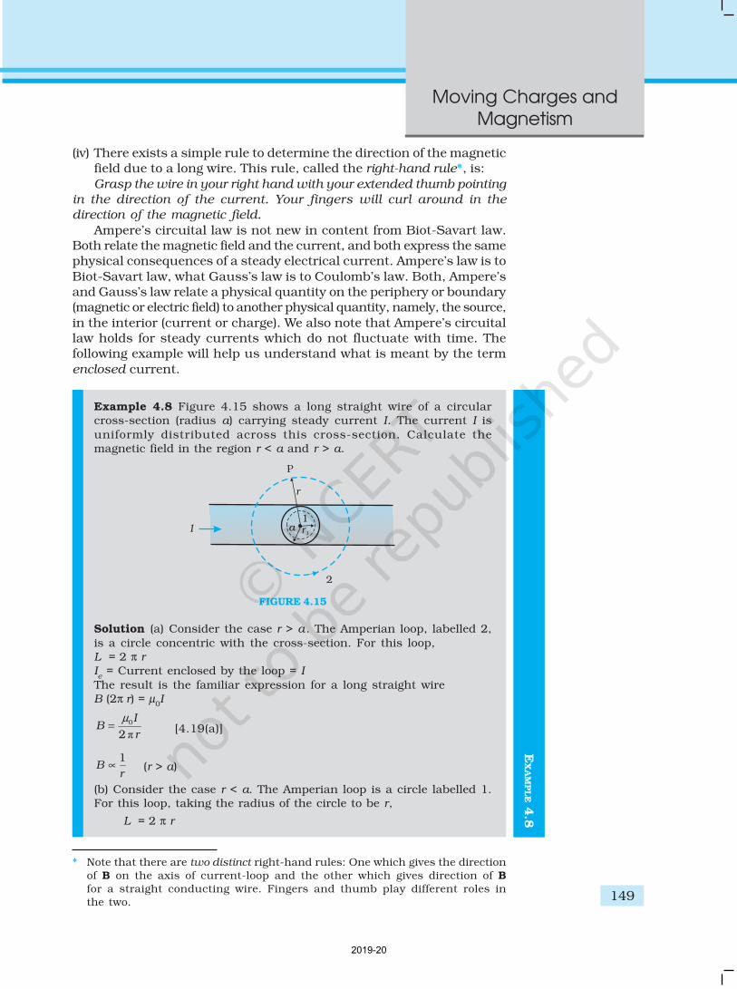
Example 4.8 Figure 4.15 shows a long straight wire of a circularcross-section (radius a) carrying steady current I. The current I is

uniformly distributed across this cross-section. Calculate themagnetic field in the region r < a and r > a.

FIGURE 4.15

Solution (a) Consider the case r > a . The Amperian loop, labelled 2,

is a circle concentric with the cross-section. For this loop,L = 2 π rIe = Current enclosed by the loop = I

The result is the familiar expression for a long straight wireB (2π r) = µ

0I

π

0

2

IB

r

µ= [4.19(a)]

1B

r∝ (r > a)

(b) Consider the case r < a. The Amperian loop is a circle labelled 1.For this loop, taking the radius of the circle to be r,

L = 2 π r

* Note that there are two distinct right-hand rules: One which gives the direction

of B on the axis of current-loop and the other which gives direction of Bfor a straight conducting wire. Fingers and thumb play different roles in

the two.

2019-20

Physics

150

EX

AM

PLE 4

.8

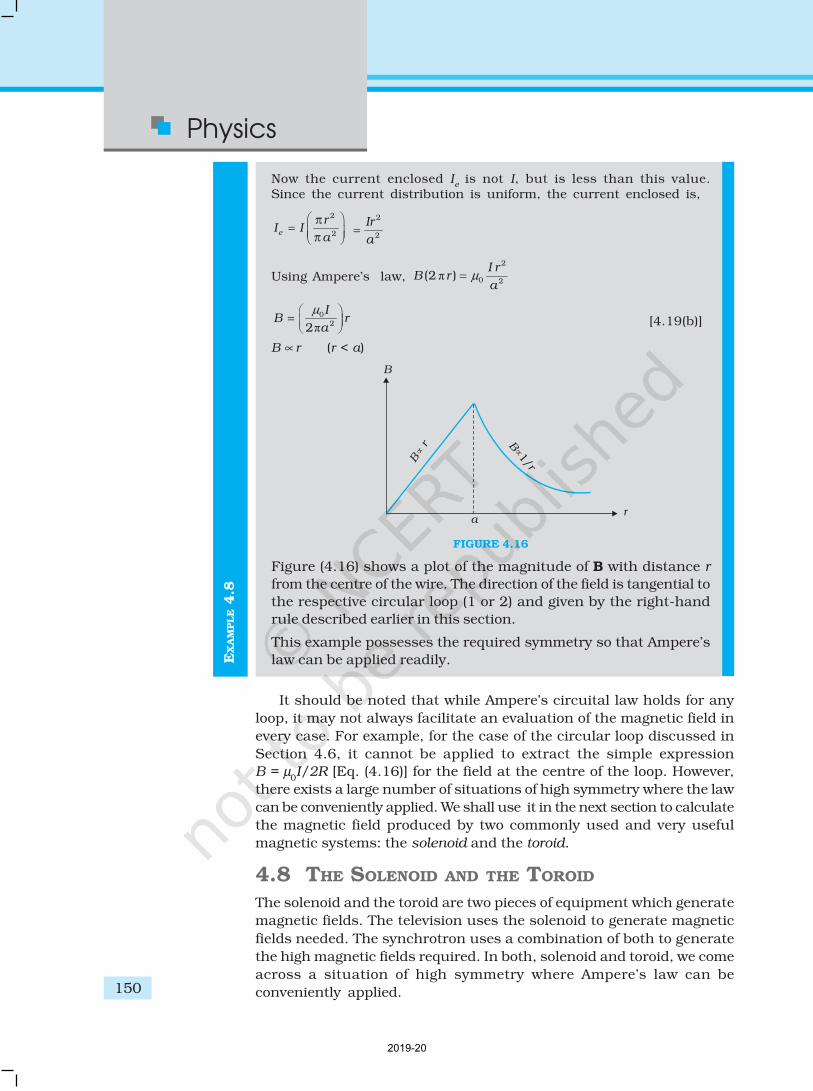
Now the current enclosed Ie is not I, but is less than this value.

Since the current distribution is uniform, the current enclosed is,

2

2

π= π e

rI I

a

2

2

Ir

a=

Using Ampere’s law, π

2

0 2(2 )

I rB r

aµ=

π

022

µ = I

B ra

[4.19(b)]

B ∝ r (r < a)

FIGURE 4.16

Figure (4.16) shows a plot of the magnitude of B with distance r

from the centre of the wire. The direction of the field is tangential to

the respective circular loop (1 or 2) and given by the right-hand

rule described earlier in this section.

This example possesses the required symmetry so that Ampere’s

law can be applied readily.

It should be noted that while Ampere’s circuital law holds for any

loop, it may not always facilitate an evaluation of the magnetic field in

every case. For example, for the case of the circular loop discussed in

Section 4.6, it cannot be applied to extract the simple expression

B = µ0I/2R [Eq. (4.16)] for the field at the centre of the loop. However,

there exists a large number of situations of high symmetry where the law

can be conveniently applied. We shall use it in the next section to calculate

the magnetic field produced by two commonly used and very useful

magnetic systems: the solenoid and the toroid.

4.8 THE SOLENOID AND THE TOROID

The solenoid and the toroid are two pieces of equipment which generate

magnetic fields. The television uses the solenoid to generate magnetic

fields needed. The synchrotron uses a combination of both to generate

the high magnetic fields required. In both, solenoid and toroid, we come

across a situation of high symmetry where Ampere’s law can be

conveniently applied.

2019-20

Moving Charges and

Magnetism

151

4.8.1 The solenoid

We shall discuss a long solenoid. By long solenoid we mean that thesolenoid’s length is large compared to its radius. It consists of a longwire wound in the form of a helix where the neighbouring turns are closely

spaced. So each turn can be regarded as a circular loop. The net magneticfield is the vector sum of the fields due to all the turns. Enamelled wiresare used for winding so that turns are insulated from each other.

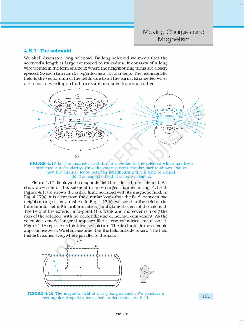
Figure 4.17 displays the magnetic field lines for a finite solenoid. Weshow a section of this solenoid in an enlarged manner in Fig. 4.17(a).Figure 4.17(b) shows the entire finite solenoid with its magnetic field. InFig. 4.17(a), it is clear from the circular loops that the field between twoneighbouring turns vanishes. In Fig. 4.17(b), we see that the field at theinterior mid-point P is uniform, strong and along the axis of the solenoid.The field at the exterior mid-point Q is weak and moreover is along theaxis of the solenoid with no perpendicular or normal component. As thesolenoid is made longer it appears like a long cylindrical metal sheet.Figure 4.18 represents this idealised picture. The field outside the solenoidapproaches zero. We shall assume that the field outside is zero. The fieldinside becomes everywhere parallel to the axis.

FIGURE 4.17 (a) The magnetic field due to a section of the solenoid which has beenstretched out for clarity. Only the exterior semi-circular part is shown. Notice

how the circular loops between neighbouring turns tend to cancel.(b) The magnetic field of a finite solenoid.

FIGURE 4.18 The magnetic field of a very long solenoid. We consider arectangular Amperian loop abcd to determine the field.

2019-20

Physics

152

Consider a rectangular Amperian loop abcd. Along cd the field is zeroas argued above. Along transverse sections bc and ad, the field component

is zero. Thus, these two sections make no contribution. Let the field alongab be B. Thus, the relevant length of the Amperian loop is, L = h.

Let n be the number of turns per unit length, then the total number

of turns is nh. The enclosed current is, Ie

= I (n h), where I is the currentin the solenoid. From Ampere’s circuital law [Eq. 4.17 (b)]

BL = µ0Ie, B h = µ

0I (n h)

B = µ0 n I (4.20)

The direction of the field is given by the right-hand rule. The solenoidis commonly used to obtain a uniform magnetic field. We shall see in the

next chapter that a large field is possible by inserting a soft

iron core inside the solenoid.

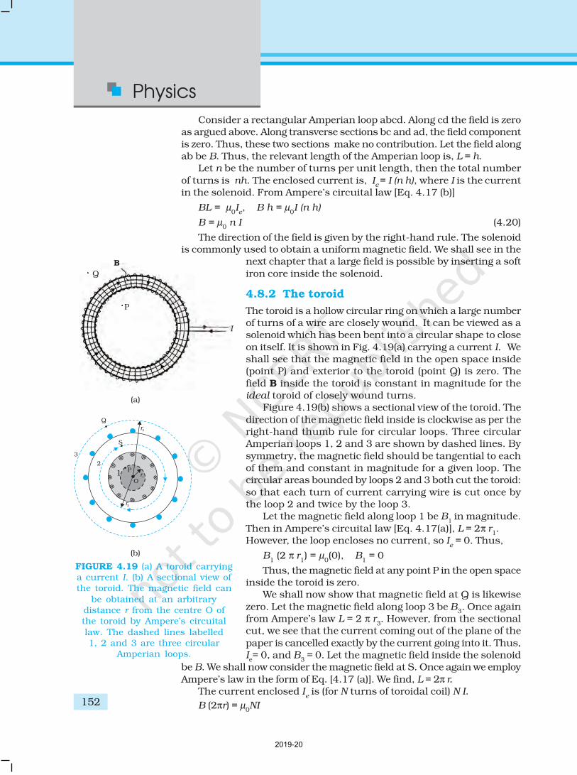
4.8.2 The toroid

The toroid is a hollow circular ring on which a large numberof turns of a wire are closely wound. It can be viewed as asolenoid which has been bent into a circular shape to close

on itself. It is shown in Fig. 4.19(a) carrying a current I. Weshall see that the magnetic field in the open space inside(point P) and exterior to the toroid (point Q) is zero. The

field B inside the toroid is constant in magnitude for theideal toroid of closely wound turns.

Figure 4.19(b) shows a sectional view of the toroid. The

direction of the magnetic field inside is clockwise as per theright-hand thumb rule for circular loops. Three circularAmperian loops 1, 2 and 3 are shown by dashed lines. By

symmetry, the magnetic field should be tangential to eachof them and constant in magnitude for a given loop. Thecircular areas bounded by loops 2 and 3 both cut the toroid:

so that each turn of current carrying wire is cut once bythe loop 2 and twice by the loop 3.

Let the magnetic field along loop 1 be B1 in magnitude.

Then in Ampere’s circuital law [Eq. 4.17(a)], L = 2π r1.

However, the loop encloses no current, so Ie = 0. Thus,

B1 (2 π r

1) = µ

0(0), B

1 = 0

Thus, the magnetic field at any point P in the open spaceinside the toroid is zero.

We shall now show that magnetic field at Q is likewise

zero. Let the magnetic field along loop 3 be B3. Once again

from Ampere’s law L = 2 π r3. However, from the sectional

cut, we see that the current coming out of the plane of the

paper is cancelled exactly by the current going into it. Thus,Ie= 0, and B

3 = 0. Let the magnetic field inside the solenoid

be B. We shall now consider the magnetic field at S. Once again we employ

Ampere’s law in the form of Eq. [4.17 (a)]. We find, L = 2π r.

The current enclosed Ie is (for N turns of toroidal coil) N I.

B (2πr) = µ0NI

FIGURE 4.19 (a) A toroid carryinga current I. (b) A sectional view ofthe toroid. The magnetic field can

be obtained at an arbitrarydistance r from the centre O ofthe toroid by Ampere’s circuital

law. The dashed lines labelled1, 2 and 3 are three circular

Amperian loops.

2019-20

Moving Charges and

Magnetism

153

0

2

NIB

r

µ=

π(4.21)

We shall now compare the two results: for a toroid and solenoid. We

re-express Eq. (4.21) to make the comparison easier with the solenoidresult given in Eq. (4.20). Let r be the average radius of the toroid and nbe the number of turns per unit length. Then

N = 2πr n = (average) perimeter of the toroid

× number of turns per unit length

and thus,

B = µ0 n I, (4.22)

i.e., the result for the solenoid!In an ideal toroid the coils are circular. In reality the turns of the

toroidal coil form a helix and there is always a small magnetic field externalto the toroid.

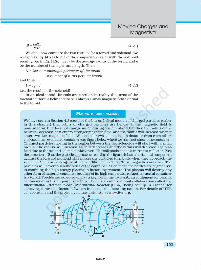
MAGNETIC CONFINEMENT

We have seen in Section 4.3 (see also the box on helical motion of charged particles earlierin this chapter) that orbits of charged particles are helical. If the magnetic field isnon-uniform, but does not change much during one circular orbit, then the radius of thehelix will decrease as it enters stronger magnetic field and the radius will increase when itenters weaker magnetic fields. We consider two solenoids at a distance from each other,enclosed in an evacuated container (see figure below where we have not shown the container).Charged particles moving in the region between the two solenoids will start with a smallradius. The radius will increase as field decreases and the radius will decrease again asfield due to the second solenoid takes over. The solenoids act as a mirror or reflector. [Seethe direction of F as the particle approaches coil 2 in the figure. It has a horizontal componentagainst the forward motion.] This makes the particles turn back when they approach thesolenoid. Such an arrangement will act like magnetic bottle or magnetic container. Theparticles will never touch the sides of the container. Such magnetic bottles are of great usein confining the high energy plasma in fusion experiments. The plasma will destroy anyother form of material container because of its high temperature. Another useful containeris a toroid. Toroids are expected to play a key role in the tokamak, an equipment for plasmaconfinement in fusion power reactors. There is an international collaboration called theInternational Thermonuclear Experimental Reactor (ITER), being set up in France, forachieving controlled fusion, of which India is a collaborating nation. For details of ITERcollaboration and the project, you may visit http://www.iter.org.

2019-20

Physics

154

EX

AM

PLE 4

.9

Example 4.9 A solenoid of length 0.5 m has a radius of 1 cm and ismade up of 500 turns. It carries a current of 5 A. What is the

magnitude of the magnetic field inside the solenoid?

Solution The number of turns per unit length is,

5001000

0.5n = = turns/m

The length l = 0.5 m and radius r = 0.01 m. Thus, l/a = 50 i.e., l >> a .

Hence, we can use the long solenoid formula, namely, Eq. (4.20)B = µ

0n I

= 4π × 10–7 × 103 × 5

= 6.28 × 10–3 T

4.9 FORCE BETWEEN TWO PARALLEL CURRENTS,THE AMPERE

We have learnt that there exists a magnetic field due to a conductor

carrying a current which obeys the Biot-Savart law. Further, we have

learnt that an external magnetic field will exert a force on

a current-carrying conductor. This follows from the

Lorentz force formula. Thus, it is logical to expect that

two current-carrying conductors placed near each other

will exert (magnetic) forces on each other. In the period

1820-25, Ampere studied the nature of this magnetic

force and its dependence on the magnitude of the current,

on the shape and size of the conductors, as well as, the

distances between the conductors. In this section, we

shall take the simple example of two parallel current-

carrying conductors, which will perhaps help us to

appreciate Ampere’s painstaking work.

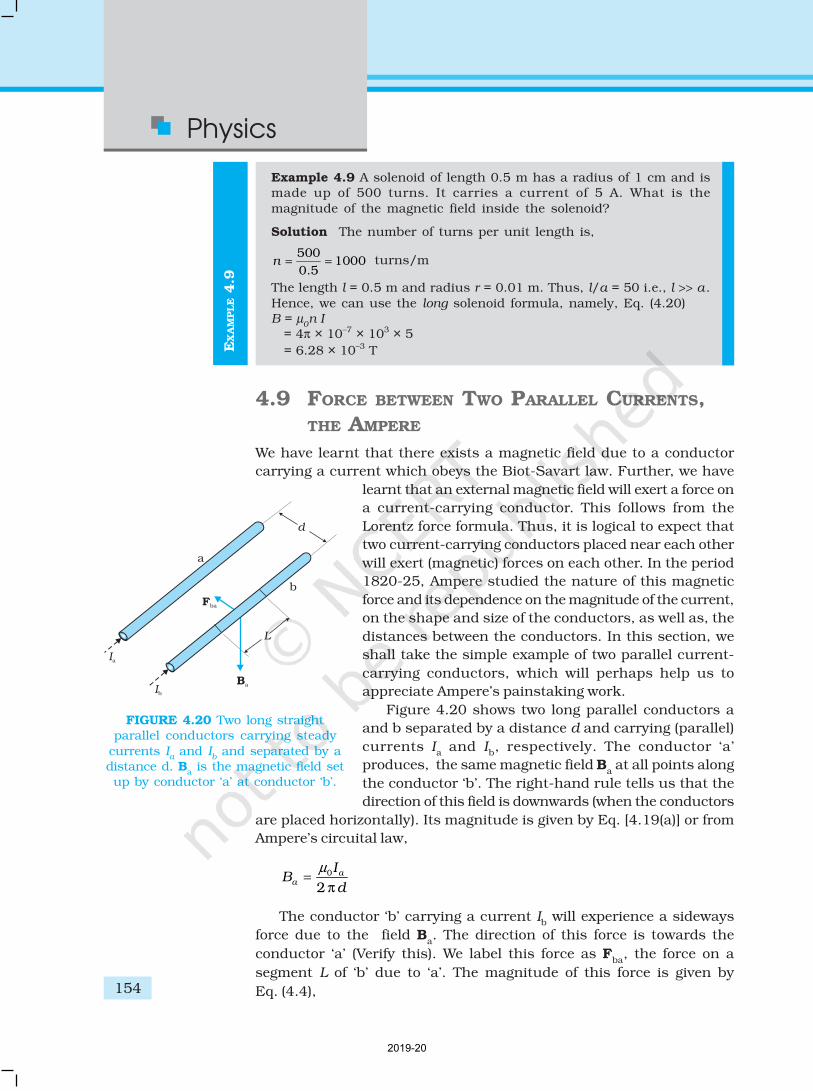
Figure 4.20 shows two long parallel conductors a

and b separated by a distance d and carrying (parallel)

currents Ia and I

b, respectively. The conductor ‘a’

produces, the same magnetic field Ba at all points along

the conductor ‘b’. The right-hand rule tells us that the

direction of this field is downwards (when the conductors

are placed horizontally). Its magnitude is given by Eq. [4.19(a)] or from

Ampere’s circuital law,

0

2a

a

IB

d

µ=

π

The conductor ‘b’ carrying a current Ib will experience a sideways

force due to the field Ba. The direction of this force is towards the

conductor ‘a’ (Verify this). We label this force as Fba

, the force on a

segment L of ‘b’ due to ‘a’. The magnitude of this force is given by

Eq. (4.4),

FIGURE 4.20 Two long straightparallel conductors carrying steady

currents Ia and I

b and separated by a

distance d. Ba is the magnetic field set

up by conductor ‘a’ at conductor ‘b’.

2019-20

Moving Charges and

Magnetism

155

Fba

= Ib L B

a

0

2a bI I

Ld

µ=

π(4.23)

It is of course possible to compute the force on ‘a’ due to ‘b’. Fromconsiderations similar to above we can find the force F

ab, on a segment of

length L of ‘a’ due to the current in ‘b’. It is equal in magnitude to Fba

,and directed towards ‘b’. Thus,

Fba

= –Fab

(4.24)

Note that this is consistent with Newton’s third Law. Thus, at least for

parallel conductors and steady currents, we have shown that the

Biot-Savart law and the Lorentz force yield results in accordance with

Newton’s third Law*.

We have seen from above that currents flowing in the same direction

attract each other. One can show that oppositely directed currents repel

each other. Thus,

Parallel currents attract, and antiparallel currents repel.

This rule is the opposite of what we find in electrostatics. Like (same

sign) charges repel each other, but like (parallel) currents attract each

other.

Let fba

represent the magnitude of the force Fba

per unit length. Then,

from Eq. (4.23),

π

0

2a b

ba

I If

d

µ= (4.25)

The above expression is used to define the ampere (A), which is one

of the seven SI base units.

The ampere is the value of that steady current which, when maintained

in each of the two very long, straight, parallel conductors of negligible

cross-section, and placed one metre apart in vacuum, would produce

on each of these conductors a force equal to 2 × 10–7 newtons per metre

of length.

This definition of the ampere was adopted in 1946. It is a theoretical

definition. In practice, one must eliminate the effect of the earth’s magnetic

field and substitute very long wires by multiturn coils of appropriate

geometries. An instrument called the current balance is used to measure

this mechanical force.

The SI unit of charge, namely, the coulomb, can now be defined in

terms of the ampere.

When a steady current of 1A is set up in a conductor, the quantity of

charge that flows through its cross-section in 1s is one coulomb (1C).

* It turns out that when we have time-dependent currents and/or charges in

motion, Newton’s third law may not hold for forces between charges and/or

conductors. An essential consequence of the Newton’s third law in mechanics

is conservation of momentum of an isolated system. This, however, holds even

for the case of time-dependent situations with electromagnetic fields, provided

the momentum carried by fields is also taken into account.

2019-20

Physics

156 EX

AM

PLE 4

.10

Example 4.10 The horizontal component of the earth’s magnetic field

at a certain place is 3.0 ×10–5 T and the direction of the field is fromthe geographic south to the geographic north. A very long straightconductor is carrying a steady current of 1A. What is the force per

unit length on it when it is placed on a horizontal table and thedirection of the current is (a) east to west; (b) south to north?

Solution F = Il × B

F = IlB sinθ

The force per unit length isf = F/l = I B sinθ

(a) When the current is flowing from east to west,θ = 90°Hence,

f = I B = 1 × 3 × 10–5 = 3 × 10–5 N m–1

ROGET’S SPIRAL FOR ATTRACTION BETWEEN PARALLEL CURRENTS

Magnetic effects are generally smaller than electric effects. As a consequence, the forcebetween currents is rather small, because of the smallness of the factor µ. Hence it isdifficult to demonstrate attraction or repulsion between currents. Thus, for 5 A current

in each wire at a separation of 1cm, the force per metre would be 5 × 10–4 N, which isabout 50 mg weight. It would be like pulling a wire by a string going over a pulley towhich a 50 mg weight is attached. The displacement of the wire would be quite

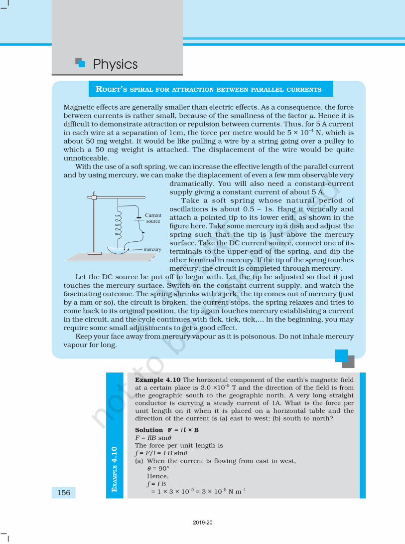
unnoticeable.With the use of a soft spring, we can increase the effective length of the parallel current

and by using mercury, we can make the displacement of even a few mm observable very

dramatically. You will also need a constant-currentsupply giving a constant current of about 5 A.

Take a soft spring whose natural period of

oscillations is about 0.5 – 1s. Hang it vertically andattach a pointed tip to its lower end, as shown in thefigure here. Take some mercury in a dish and adjust the

spring such that the tip is just above the mercurysurface. Take the DC current source, connect one of itsterminals to the upper end of the spring, and dip the

other terminal in mercury. If the tip of the spring touchesmercury, the circuit is completed through mercury.

Let the DC source be put off to begin with. Let the tip be adjusted so that it just

touches the mercury surface. Switch on the constant current supply, and watch thefascinating outcome. The spring shrinks with a jerk, the tip comes out of mercury (justby a mm or so), the circuit is broken, the current stops, the spring relaxes and tries to

come back to its original position, the tip again touches mercury establishing a currentin the circuit, and the cycle continues with tick, tick, tick,... In the beginning, you mayrequire some small adjustments to get a good effect.

Keep your face away from mercury vapour as it is poisonous. Do not inhale mercuryvapour for long.

2019-20

Moving Charges and

Magnetism

157

EX

AM

PLE 4

.10

This is larger than the value 2×10–7 Nm–1 quoted in the definitionof the ampere. Hence it is important to eliminate the effect of the

earth’s magnetic field and other stray fields while standardisingthe ampere.The direction of the force is downwards. This direction may be

obtained by the directional property of cross product of vectors.(b) When the current is flowing from south to north,

θ = 0o

f = 0Hence there is no force on the conductor.

4.10 TORQUE ON CURRENT LOOP, MAGNETIC DIPOLE

4.10.1 Torque on a rectangular current loop in a uniformmagnetic field

We now show that a rectangular loop carrying a steady current I and

placed in a uniform magnetic field experiences a torque. It does notexperience a net force. This behaviour is analogous to

that of electric dipole in a uniform electric field

(Section 1.12).

We first consider the simple case when therectangular loop is placed such that the uniform

magnetic field B is in the plane of the loop. This is

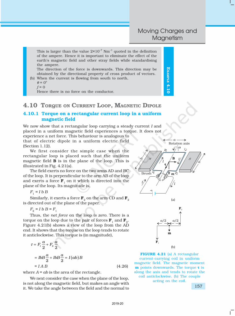
illustrated in Fig. 4.21(a).The field exerts no force on the two arms AD and BC

of the loop. It is perpendicular to the arm AB of the loop

and exerts a force F1 on it which is directed into the

plane of the loop. Its magnitude is,

F1 = I b B

Similarly, it exerts a force F2 on the arm CD and F

2

is directed out of the plane of the paper.

F2 = I b B = F

1

Thus, the net force on the loop is zero. There is a

torque on the loop due to the pair of forces F1 and F

2.

Figure 4.21(b) shows a view of the loop from the AD

end. It shows that the torque on the loop tends to rotateit anticlockwise. This torque is (in magnitude),

1 22 2

a aF Fτ = +

( )2 2

a aIbB IbB I ab B= + =

= I A B (4.26)

where A = ab is the area of the rectangle.

We next consider the case when the plane of the loop,

is not along the magnetic field, but makes an angle withit. We take the angle between the field and the normal to

FIGURE 4.21 (a) A rectangularcurrent-carrying coil in uniform

magnetic field. The magnetic moment

m points downwards. The torque τττττ isalong the axis and tends to rotate the

coil anticlockwise. (b) The couple

acting on the coil.

2019-20

Physics

158

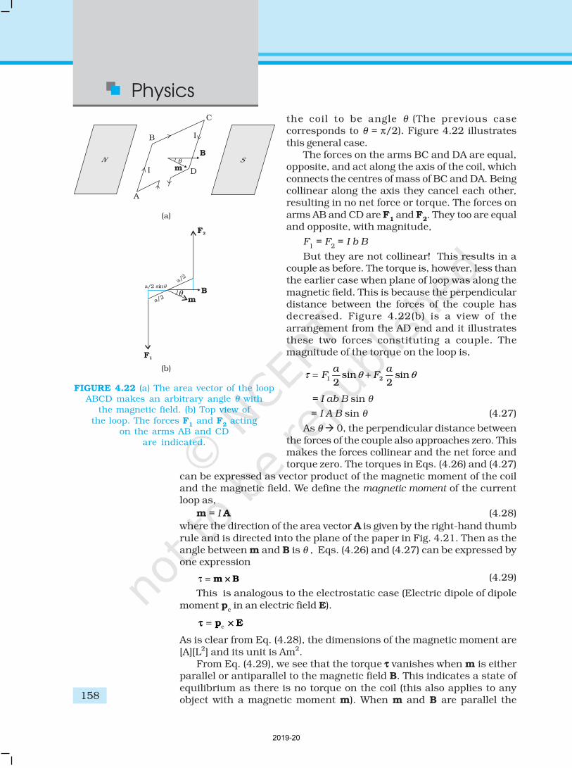
the coil to be angle θ (The previous casecorresponds to θ = π/2). Figure 4.22 illustrates

this general case.The forces on the arms BC and DA are equal,

opposite, and act along the axis of the coil, which

connects the centres of mass of BC and DA. Beingcollinear along the axis they cancel each other,resulting in no net force or torque. The forces on

arms AB and CD are F1 and F

2. They too are equal

and opposite, with magnitude,

F1 = F

2 = I b B

But they are not collinear! This results in acouple as before. The torque is, however, less thanthe earlier case when plane of loop was along the

magnetic field. This is because the perpendiculardistance between the forces of the couple hasdecreased. Figure 4.22(b) is a view of the

arrangement from the AD end and it illustratesthese two forces constituting a couple. Themagnitude of the torque on the loop is,

1 2sin sin2 2

a aF Fτ θ θ= +

= I ab B sin θ

= I A B sin θ (4.27)

As θ à 0, the perpendicular distance between

the forces of the couple also approaches zero. Thismakes the forces collinear and the net force andtorque zero. The torques in Eqs. (4.26) and (4.27)

can be expressed as vector product of the magnetic moment of the coiland the magnetic field. We define the magnetic moment of the currentloop as,

m = I A (4.28)

where the direction of the area vector A is given by the right-hand thumb

rule and is directed into the plane of the paper in Fig. 4.21. Then as theangle between m and B is θ , Eqs. (4.26) and (4.27) can be expressed byone expression

τ = m B×× (4.29)

This is analogous to the electrostatic case (Electric dipole of dipole

moment pe in an electric field E).

ττ ××= p Ee

As is clear from Eq. (4.28), the dimensions of the magnetic moment are

[A][L2] and its unit is Am2.From Eq. (4.29), we see that the torque τττττ vanishes when m is either

parallel or antiparallel to the magnetic field B. This indicates a state of

equilibrium as there is no torque on the coil (this also applies to anyobject with a magnetic moment m). When m and B are parallel the

FIGURE 4.22 (a) The area vector of the loopABCD makes an arbitrary angle θ with

the magnetic field. (b) Top view of

the loop. The forces F1 and F

2 acting

on the arms AB and CDare indicated.

2019-20

Moving Charges and

Magnetism

159

EX

AM

PLE 4

.11

equilibrium is a stable one. Any small rotation of the coil produces atorque which brings it back to its original position. When they are

antiparallel, the equilibrium is unstable as any rotation produces a torquewhich increases with the amount of rotation. The presence of this torqueis also the reason why a small magnet or any magnetic dipole aligns

itself with the external magnetic field.If the loop has N closely wound turns, the expression for torque, Eq.

(4.29), still holds, with

m = N I A (4.30)

Example 4.11 A 100 turn closely wound circular coil of radius 10 cmcarries a current of 3.2 A. (a) What is the field at the centre of thecoil? (b) What is the magnetic moment of this coil?

The coil is placed in a vertical plane and is free to rotate about ahorizontal axis which coincides with its diameter. A uniform magneticfield of 2T in the horizontal direction exists such that initially the

axis of the coil is in the direction of the field. The coil rotates throughan angle of 90° under the influence of the magnetic field.(c) What are the magnitudes of the torques on the coil in the initial

and final position? (d) What is the angular speed acquired by thecoil when it has rotated by 90°? The moment of inertia of the coil is0.1 kg m2.

Solution(a) From Eq. (4.16)

BNI

R=

µ0

2Here, N = 100; I = 3.2 A, and R = 0.1 m. Hence,

B =× × ×

×

−

−

4 10 10 3 2

2 10

7 2

1

π . =

× ×

×

−

−

4 10 10

2 10

5

1 (using π × 3.2 = 10)

= 2 × 10–3 TThe direction is given by the right-hand thumb rule.

(b) The magnetic moment is given by Eq. (4.30),

m = N I A = N I π r2 = 100 × 3.2 × 3.14 × 10–2 = 10 A m2

The direction is once again given by the right-hand thumb rule.

(c) τ = m B× [from Eq. (4.29)]

sinm B θ=

Initially, θ = 0. Thus, initial torque τi = 0. Finally, θ = π/2 (or 90º).

Thus, final torque τf = m B = 10 × 2 = 20 N m.

(d) From Newton’s second law,

I

where I is the moment of inertia of the coil. From chain rule,

Using this,

I

2019-20

Physics

160

EX

AM

PLE 4

.12

EX

AM

PLE 4

.11

Example 4.12

(a) A current-carrying circular loop lies on a smooth horizontal plane.Can a uniform magnetic field be set up in such a manner thatthe loop turns around itself (i.e., turns about the vertical axis).

(b) A current-carrying circular loop is located in a uniform externalmagnetic field. If the loop is free to turn, what is its orientationof stable equilibrium? Show that in this orientation, the flux of

the total field (external field + field produced by the loop) ismaximum.

(c) A loop of irregular shape carrying current is located in an external

magnetic field. If the wire is flexible, why does it change to acircular shape?

Solution

(a) No, because that would require τττττ to be in the vertical direction.But τττττ = I A × B, and since A of the horizontal loop is in the verticaldirection, τ would be in the plane of the loop for any B.

(b) Orientation of stable equilibrium is one where the area vector Aof the loop is in the direction of external magnetic field. In thisorientation, the magnetic field produced by the loop is in the same

direction as external field, both normal to the plane of the loop,thus giving rise to maximum flux of the total field.

(c) It assumes circular shape with its plane normal to the field to

maximise flux, since for a given perimeter, a circle encloses greater

area than any other shape.

4.10.2 Circular current loop as a magnetic dipole

In this section, we shall consider the elementary magnetic element: thecurrent loop. We shall show that the magnetic field (at large distances)

due to current in a circular current loop is very similar in behaviour tothe electric field of an electric dipole. In Section 4.6, we have evaluatedthe magnetic field on the axis of a circular loop, of a radius R, carrying a

steady current I. The magnitude of this field is [(Eq. (4.15)],

( )

20

3/22 22

µ=

+

I RB

x R

and its direction is along the axis and given by the right-hand thumbrule (Fig. 4.12). Here, x is the distance along the axis from the centre of

the loop. For x >> R, we may drop the R2 term in the denominator. Thus,

Integrating from θ = 0 to θ = π/2,

2019-20

Moving Charges and

Magnetism

161

20

32

IRB

x

µ=

Note that the area of the loop A = πR2. Thus,

0

32

IAB

x

µ=

π

As earlier, we define the magnetic moment m to have a magnitude IA,

m = I A. Hence,

Bm

;µ

0

32 πx

π

0

3

2

4 x

µ=

m[4.31(a)]

The expression of Eq. [4.31(a)] is very similar to an expression obtainedearlier for the electric field of a dipole. The similarity may be seen if wesubstitute,

0 01/µ ε→

e→m p (electrostatic dipole)

→B E (electrostatic field)

We then obtain,

30

2

4e

xε=

π

pE

which is precisely the field for an electric dipole at a point on its axis.considered in Chapter 1, Section 1.10 [Eq. (1.20)].

It can be shown that the above analogy can be carried further. Wehad found in Chapter 1 that the electric field on the perpendicular bisectorof the dipole is given by [See Eq.(1.21)],

E ;p

e

x40

3πε

where x is the distance from the dipole. If we replace p à m and 0 01/µ ε→

in the above expression, we obtain the result for B for a point in the

plane of the loop at a distance x from the centre. For x >>R,

Bm

;µ

0

34π x

x R; >> [4.31(b)]

The results given by Eqs. [4.31(a)] and [4.31(b)] become exact for a

point magnetic dipole.The results obtained above can be shown to apply to any planar loop:

a planar current loop is equivalent to a magnetic dipole of dipole moment

m = I A, which is the analogue of electric dipole moment p. Note, however,a fundamental difference: an electric dipole is built up of two elementaryunits — the charges (or electric monopoles). In magnetism, a magnetic

dipole (or a current loop) is the most elementary element. The equivalentof electric charges, i.e., magnetic monopoles, are not known to exist.

We have shown that a current loop (i) produces a magnetic field (see

Fig. 4.12) and behaves like a magnetic dipole at large distances, and

2019-20

Physics

162

(ii) is subject to torque like a magnetic needle. This led Ampere to suggestthat all magnetism is due to circulating currents. This seems to be partly

true and no magnetic monopoles have been seen so far. However,elementary particles such as an electron or a proton also carry an intrinsic

magnetic moment, not accounted by circulating currents.

4.10.3 The magnetic dipole moment of a revolving electron

In Chapter 12 we shall read about the Bohr model of the hydrogen atom.You may perhaps have heard of this model which was proposed by the

Danish physicist Niels Bohr in 1911 and was a stepping stone

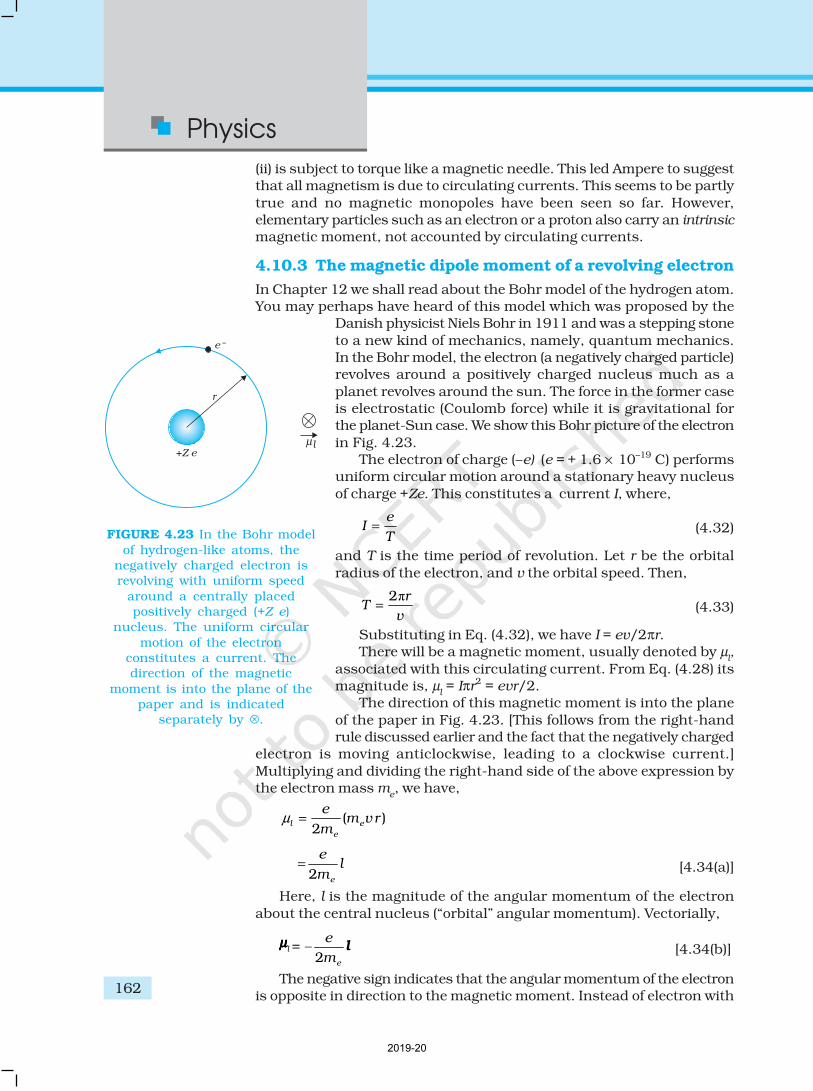
to a new kind of mechanics, namely, quantum mechanics.In the Bohr model, the electron (a negatively charged particle)revolves around a positively charged nucleus much as a

planet revolves around the sun. The force in the former caseis electrostatic (Coulomb force) while it is gravitational forthe planet-Sun case. We show this Bohr picture of the electron

in Fig. 4.23.The electron of charge (–e) (e = + 1.6 × 10–19 C) performs

uniform circular motion around a stationary heavy nucleus

of charge +Ze. This constitutes a current I, where,

eI

T= (4.32)

and T is the time period of revolution. Let r be the orbital

radius of the electron, and v the orbital speed. Then,

π2 rT =

v(4.33)

Substituting in Eq. (4.32), we have I = ev/2πr.There will be a magnetic moment, usually denoted by µ

l,

associated with this circulating current. From Eq. (4.28) itsmagnitude is, µ

l = Iπr2 = evr/2.

The direction of this magnetic moment is into the plane

of the paper in Fig. 4.23. [This follows from the right-handrule discussed earlier and the fact that the negatively charged

electron is moving anticlockwise, leading to a clockwise current.]

Multiplying and dividing the right-hand side of the above expression bythe electron mass m

e, we have,

( )2

l e

e

em vr

mµ =

2 e

el

m= [4.34(a)]

Here, l is the magnitude of the angular momentum of the electron

about the central nucleus (“orbital” angular momentum). Vectorially,

µµµµµl = –

2l

e

e

ml [4.34(b)]

The negative sign indicates that the angular momentum of the electronis opposite in direction to the magnetic moment. Instead of electron with

FIGURE 4.23 In the Bohr model

of hydrogen-like atoms, thenegatively charged electron isrevolving with uniform speed

around a centrally placedpositively charged (+Z e)

nucleus. The uniform circular

motion of the electronconstitutes a current. Thedirection of the magnetic

moment is into the plane of thepaper and is indicated

separately by ⊗.

2019-20

Moving Charges and

Magnetism

163

charge (–e), if we had taken a particle with charge (+q), the angularmomentum and magnetic moment would be in the same direction. The

ratio

l

2 e

e

l m

µ= (4.35)

is called the gyromagnetic ratio and is a constant. Its value is 8.8 × 1010 C /kgfor an electron, which has been verified by experiments.

The fact that even at an atomic level there is a magnetic moment,

confirms Ampere’s bold hypothesis of atomic magnetic moments. Thisaccording to Ampere, would help one to explain the magnetic propertiesof materials. Can one assign a value to this atomic dipole moment? The

answer is Yes. One can do so within the Bohr model. Bohr hypothesisedthat the angular momentum assumes a discrete set of values, namely,

2

n hl =

π(4.36)

where n is a natural number, n = 1, 2, 3, .... and h is a constant named

after Max Planck (Planck’s constant) with a value h = 6.626 × 10–34 J s.

This condition of discreteness is called the Bohr quantisation condition.

We shall discuss it in detail in Chapter 12. Our aim here is merely to use

it to calculate the elementary dipole moment. Take the value n = 1, we

have from Eq. (4.34) that,

min( )4

l

e

eh

mµ =

π

19 34

31

1.60 10 6.63 10

4 3.14 9.11 10

− −

−

× × ×=

× × ×

= 9.27 × 10–24 Am2 (4.37)

where the subscript ‘min’ stands for minimum. This value is called the

Bohr magneton.

Any charge in uniform circular motion would have an associated

magnetic moment given by an expression similar to Eq. (4.34). This dipole

moment is labelled as the orbital magnetic moment. Hence, the subscript

‘l’ in µl. Besides the orbital moment, the electron has an intrinsic magnetic

moment, which has the same numerical value as given in Eq. (4.37). It is

called the spin magnetic moment. But we hasten to add that it is not as

though the electron is spinning. The electron is an elementary particle

and it does not have an axis to spin around like a top or our earth.

Nevertheless, it does possess this intrinsic magnetic moment. The

microscopic roots of magnetism in iron and other materials can be traced

back to this intrinsic spin magnetic moment.

4.11 THE MOVING COIL GALVANOMETER

Currents and voltages in circuits have been discussed extensively in

Chapters 3. But how do we measure them? How do we claim thatcurrent in a circuit is 1.5 A or the voltage drop across a resistor is 1.2 V?Figure 4.24 exhibits a very useful instrument for this purpose: the moving

Co

nvers

ion

of g

alv

an

om

ete

r into

am

mete

r an

d v

oltm

ete

r:

ww

w.c

itycolle

gia

te.c

om

/galv

anom

ete

r_XIIa

.htm

2019-20

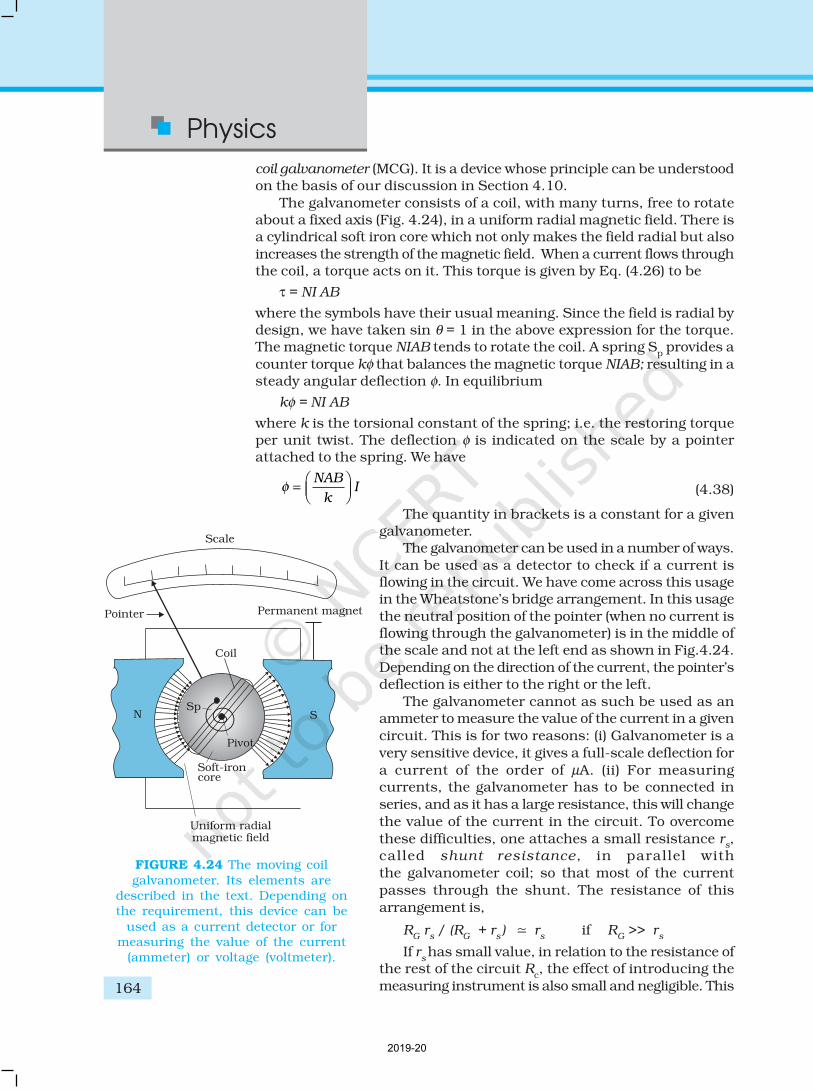
Physics

164

coil galvanometer (MCG). It is a device whose principle can be understoodon the basis of our discussion in Section 4.10.

The galvanometer consists of a coil, with many turns, free to rotateabout a fixed axis (Fig. 4.24), in a uniform radial magnetic field. There isa cylindrical soft iron core which not only makes the field radial but also

increases the strength of the magnetic field. When a current flows throughthe coil, a torque acts on it. This torque is given by Eq. (4.26) to be

τ = NI AB

where the symbols have their usual meaning. Since the field is radial bydesign, we have taken sin θ = 1 in the above expression for the torque.The magnetic torque NIAB tends to rotate the coil. A spring S

p provides a

counter torque kφ that balances the magnetic torque NIAB; resulting in asteady angular deflection φ. In equilibrium

kφ = NI AB

where k is the torsional constant of the spring; i.e. the restoring torqueper unit twist. The deflection φ is indicated on the scale by a pointerattached to the spring. We have

φ =

NAB

kI (4.38)

The quantity in brackets is a constant for a givengalvanometer.

The galvanometer can be used in a number of ways.

It can be used as a detector to check if a current isflowing in the circuit. We have come across this usagein the Wheatstone’s bridge arrangement. In this usage

the neutral position of the pointer (when no current isflowing through the galvanometer) is in the middle ofthe scale and not at the left end as shown in Fig.4.24.

Depending on the direction of the current, the pointer’sdeflection is either to the right or the left.

The galvanometer cannot as such be used as anammeter to measure the value of the current in a given

circuit. This is for two reasons: (i) Galvanometer is a

very sensitive device, it gives a full-scale deflection for

a current of the order of µA. (ii) For measuringcurrents, the galvanometer has to be connected in

series, and as it has a large resistance, this will change

the value of the current in the circuit. To overcome

these difficulties, one attaches a small resistance rs,

called shunt resistance, in parallel with

the galvanometer coil; so that most of the current

passes through the shunt. The resistance of this

arrangement is,

RG r

s / (R

G + r

s) ; r

s if R

G >> r

s

If rs has small value, in relation to the resistance of

the rest of the circuit Rc, the effect of introducing the

measuring instrument is also small and negligible. This

FIGURE 4.24 The moving coil

galvanometer. Its elements aredescribed in the text. Depending onthe requirement, this device can be

used as a current detector or formeasuring the value of the current

(ammeter) or voltage (voltmeter).

2019-20

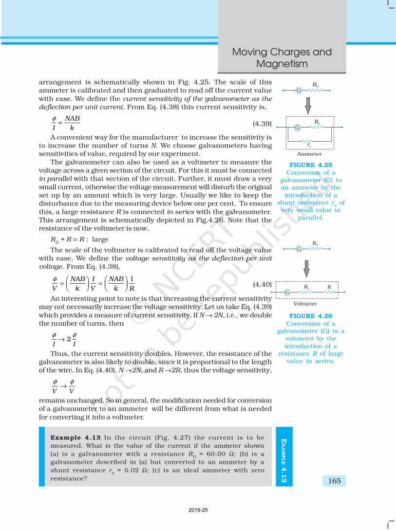
Moving Charges and

Magnetism

165

arrangement is schematically shown in Fig. 4.25. The scale of thisammeter is calibrated and then graduated to read off the current value

with ease. We define the current sensitivity of the galvanometer as the

deflection per unit current. From Eq. (4.38) this current sensitivity is,

NAB

I k

φ= (4.39)

A convenient way for the manufacturer to increase the sensitivity isto increase the number of turns N. We choose galvanometers havingsensitivities of value, required by our experiment.

The galvanometer can also be used as a voltmeter to measure thevoltage across a given section of the circuit. For this it must be connectedin parallel with that section of the circuit. Further, it must draw a very

small current, otherwise the voltage measurement will disturb the originalset up by an amount which is very large. Usually we like to keep thedisturbance due to the measuring device below one per cent. To ensure

this, a large resistance R is connected in series with the galvanometer.This arrangement is schematically depicted in Fig.4.26. Note that theresistance of the voltmeter is now,

RG + R ; R : large

The scale of the voltmeter is calibrated to read off the voltage valuewith ease. We define the voltage sensitivity as the deflection per unit

voltage. From Eq. (4.38),

φ

V

NAB

k

I

V

NAB

k R=

=

1

(4.40)

An interesting point to note is that increasing the current sensitivitymay not necessarily increase the voltage sensitivity. Let us take Eq. (4.39)

which provides a measure of current sensitivity. If N → 2N, i.e., we doublethe number of turns, then

2I I

φ φ→

Thus, the current sensitivity doubles. However, the resistance of thegalvanometer is also likely to double, since it is proportional to the lengthof the wire. In Eq. (4.40), N →2N, and R →2R, thus the voltage sensitivity,

V V

φ φ→

remains unchanged. So in general, the modification needed for conversionof a galvanometer to an ammeter will be different from what is needed

for converting it into a voltmeter.

Example 4.13 In the circuit (Fig. 4.27) the current is to be

measured. What is the value of the current if the ammeter shown

(a) is a galvanometer with a resistance RG = 60.00 Ω; (b) is a

galvanometer described in (a) but converted to an ammeter by a

shunt resistance rs = 0.02 Ω; (c) is an ideal ammeter with zero

resistance?

FIGURE 4.25

Conversion of agalvanometer (G) toan ammeter by the

introduction of ashunt resistance r

s of

very small value in

parallel.

FIGURE 4.26

Conversion of agalvanometer (G) to a

voltmeter by the

introduction of aresistance R of large

value in series.

EX

AM

PLE 4

.13

2019-20

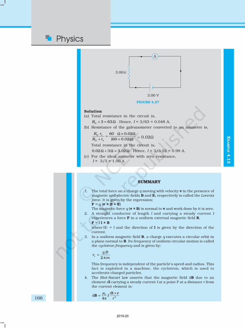
Physics

166

FIGURE 4.27

Solution(a) Total resistance in the circuit is,

3 63GR + = Ω . Hence, I = 3/63 = 0.048 A.

(b) Resistance of the galvanometer converted to an ammeter is,

R r

R r

G s

G s+=

×

+

60 0 02

60 0 02

Ω Ω

Ω

.

( . ) ; 0.02Ω

Total resistance in the circuit is,

0.02 3 3.02Ω + Ω = Ω . Hence, I = 3/3.02 = 0.99 A.

(c) For the ideal ammeter with zero resistance, I = 3/3 = 1.00 A

SUMMARY

1. The total force on a charge q moving with velocity v in the presence of

magnetic and electric fields B and E, respectively is called the Lorentz

force. It is given by the expression:F = q (v × B + E)

The magnetic force q (v × B) is normal to v and work done by it is zero.

2. A straight conductor of length l and carrying a steady current I

experiences a force F in a uniform external magnetic field B,

F = I l × B

where|l| = l and the direction of l is given by the direction of the

current.

3. In a uniform magnetic field B, a charge q executes a circular orbit in

a plane normal to B. Its frequency of uniform circular motion is called

the cyclotron frequency and is given by:

2c

q B

mν =

π

This frequency is independent of the particle’s speed and radius. This

fact is exploited in a machine, the cyclotron, which is used toaccelerate charged particles.

4. The Biot-Savart law asserts that the magnetic field dB due to an

element dl carrying a steady current I at a point P at a distance r from

the current element is:

0

3

dd

4I

r

µ ×=

π

l rB

EX

AM

PLE 4

.13

2019-20

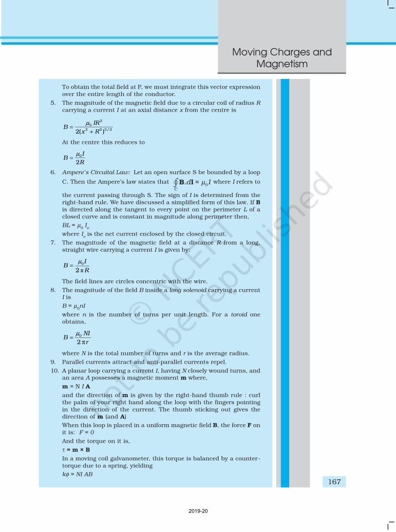
Moving Charges and

Magnetism

167

To obtain the total field at P, we must integrate this vector expression

over the entire length of the conductor.

5. The magnitude of the magnetic field due to a circular coil of radius R

carrying a current I at an axial distance x from the centre is

20

2 2 3/22( )

IRB

x R

µ=

+

At the centre this reduces to

0

2

IB

R

µ=

6. Ampere’s Circuital Law: Let an open surface S be bounded by a loop

C. Then the Ampere’s law states that B l.d I=∫ µ0

C

Ñ where I refers to

the current passing through S. The sign of I is determined from the

right-hand rule. We have discussed a simplified form of this law. If Bis directed along the tangent to every point on the perimeter L of a

closed curve and is constant in magnitude along perimeter then,

BL = µ0 I

e

where Ie is the net current enclosed by the closed circuit.

7. The magnitude of the magnetic field at a distance R from a long,

straight wire carrying a current I is given by:

π

0

2

IB

R

µ=

The field lines are circles concentric with the wire.

8. The magnitude of the field B inside a long solenoid carrying a currentI is

B = µ0nI

where n is the number of turns per unit length. For a toroid one

obtains,

0

2

NIB

r

µ=

π

where N is the total number of turns and r is the average radius.

9. Parallel currents attract and anti-parallel currents repel.

10. A planar loop carrying a current I, having N closely wound turns, andan area A possesses a magnetic moment m where,

m = N I A

and the direction of m is given by the right-hand thumb rule : curl

the palm of your right hand along the loop with the fingers pointing

in the direction of the current. The thumb sticking out gives the

direction of m (and A)

When this loop is placed in a uniform magnetic field B, the force F on

it is: F = 0

And the torque on it is,

τ = m × B

In a moving coil galvanometer, this torque is balanced by a counter-

torque due to a spring, yielding

kφ = NI AB

2019-20

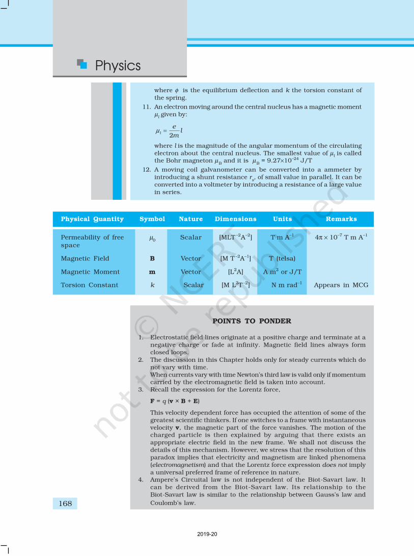
Physics

168

where φ is the equilibrium deflection and k the torsion constant of

the spring.

11. An electron moving around the central nucleus has a magnetic moment

µl given by:

2l

el

mµ =

where l is the magnitude of the angular momentum of the circulating

electron about the central nucleus. The smallest value of µl is called

the Bohr magneton µB and it is µ

B = 9.27×10–24 J/T

12. A moving coil galvanometer can be converted into a ammeter by

introducing a shunt resistance rs, of small value in parallel. It can be

converted into a voltmeter by introducing a resistance of a large value

in series.

Physical Quantity Symbol Nature Dimensions Units Remarks

Permeability of free µ0

Scalar [MLT –2A–2] T m A–1 4π × 10–7 T m A–1

space

Magnetic Field B Vector [M T –2A–1] T (telsa)

Magnetic Moment m Vector [L2A] A m2 or J/T

Torsion Constant k Scalar [M L2T –2] N m rad–1 Appears in MCG

POINTS TO PONDER

1. Electrostatic field lines originate at a positive charge and terminate at a

negative charge or fade at infinity. Magnetic field lines always form

closed loops.

2. The discussion in this Chapter holds only for steady currents which do

not vary with time.

When currents vary with time Newton’s third law is valid only if momentumcarried by the electromagnetic field is taken into account.

3. Recall the expression for the Lorentz force,

F = q (v × B + E)

This velocity dependent force has occupied the attention of some of the

greatest scientific thinkers. If one switches to a frame with instantaneous

velocity v, the magnetic part of the force vanishes. The motion of thecharged particle is then explained by arguing that there exists an

appropriate electric field in the new frame. We shall not discuss the

details of this mechanism. However, we stress that the resolution of this

paradox implies that electricity and magnetism are linked phenomena

(electromagnetism) and that the Lorentz force expression does not imply

a universal preferred frame of reference in nature.4. Ampere’s Circuital law is not independent of the Biot-Savart law. It

can be derived from the Biot-Savart law. Its relationship to the

Biot-Savart law is similar to the relationship between Gauss’s law and

Coulomb’s law.

2019-20

Moving Charges and

Magnetism

169

EXERCISES

4.1 A circular coil of wire consisting of 100 turns, each of radius 8.0 cm

carries a current of 0.40 A. What is the magnitude of the magneticfield B at the centre of the coil?

4.2 A long straight wire carries a current of 35 A. What is the magnitude

of the field B at a point 20 cm from the wire?

4.3 A long straight wire in the horizontal plane carries a current of 50 Ain north to south direction. Give the magnitude and direction of B

at a point 2.5 m east of the wire.

4.4 A horizontal overhead power line carries a current of 90 A in east towest direction. What is the magnitude and direction of the magnetic

field due to the current 1.5 m below the line?

4.5 What is the magnitude of magnetic force per unit length on a wirecarrying a current of 8 A and making an angle of 30º with the

direction of a uniform magnetic field of 0.15 T?

4.6 A 3.0 cm wire carrying a current of 10 A is placed inside a solenoidperpendicular to its axis. The magnetic field inside the solenoid is

given to be 0.27 T. What is the magnetic force on the wire?

4.7 Two long and parallel straight wires A and B carrying currents of8.0 A and 5.0 A in the same direction are separated by a distance of

4.0 cm. Estimate the force on a 10 cm section of wire A.

4.8 A closely wound solenoid 80 cm long has 5 layers of windings of 400turns each. The diameter of the solenoid is 1.8 cm. If the current

carried is 8.0 A, estimate the magnitude of B inside the solenoidnear its centre.

4.9 A square coil of side 10 cm consists of 20 turns and carries a current

of 12 A. The coil is suspended vertically and the normal to the planeof the coil makes an angle of 30º with the direction of a uniformhorizontal magnetic field of magnitude 0.80 T. What is the magnitude

of torque experienced by the coil?

4.10 Two moving coil meters, M1 and M

2 have the following particulars:

R1 = 10 Ω, N

1 = 30,

A1 = 3.6 × 10–3 m2, B

1 = 0.25 T

R2 = 14 Ω, N

2 = 42,

A2 = 1.8 × 10–3 m2, B

2 = 0.50 T

(The spring constants are identical for the two meters).

Determine the ratio of (a) current sensitivity and (b) voltagesensitivity of M

2 and M

1.

4.11 In a chamber, a uniform magnetic field of 6.5 G (1 G = 10–4 T) ismaintained. An electron is shot into the field with a speed of4.8 × 106 m s–1 normal to the field. Explain why the path of the

electron is a circle. Determine the radius of the circular orbit.(e = 1.5 × 10–19 C, m

e = 9.1×10–31 kg)

4.12 In Exercise 4.11 obtain the frequency of revolution of the electron in

its circular orbit. Does the answer depend on the speed of theelectron? Explain.

4.13 (a) A circular coil of 30 turns and radius 8.0 cm carrying a current

of 6.0 A is suspended vertically in a uniform horizontal magneticfield of magnitude 1.0 T. The field lines make an angle of 60°

2019-20

Physics

170

with the normal of the coil. Calculate the magnitude of thecounter torque that must be applied to prevent the coil fromturning.

(b) Would your answer change, if the circular coil in (a) were replacedby a planar coil of some irregular shape that encloses the samearea? (All other particulars are also unaltered.)

ADDITIONAL EXERCISES

4.14 Two concentric circular coils X and Y of radii 16 cm and 10 cm,respectively, lie in the same vertical plane containing the north to

south direction. Coil X has 20 turns and carries a current of 16 A;coil Y has 25 turns and carries a current of 18 A. The sense of thecurrent in X is anticlockwise, and clockwise in Y, for an observer

looking at the coils facing west. Give the magnitude and direction ofthe net magnetic field due to the coils at their centre.

4.15 A magnetic field of 100 G (1 G = 10–4 T) is required which is uniform

in a region of linear dimension about 10 cm and area of cross-sectionabout 10–3 m2. The maximum current-carrying capacity of a givencoil of wire is 15 A and the number of turns per unit length that can

be wound round a core is at most 1000 turns m–1. Suggest someappropriate design particulars of a solenoid for the required purpose.Assume the core is not ferromagnetic.

4.16 For a circular coil of radius R and N turns carrying current I, themagnitude of the magnetic field at a point on its axis at a distance xfrom its centre is given by,

( )

20

3/22 22

IR NB

x R

µ=

+

(a) Show that this reduces to the familiar result for field at thecentre of the coil.

(b) Consider two parallel co-axial circular coils of equal radius R,and number of turns N, carrying equal currents in the samedirection, and separated by a distance R. Show that the field on

the axis around the mid-point between the coils is uniform overa distance that is small as compared to R, and is given by,

00.72NI

BR

µ= , approximately.

[Such an arrangement to produce a nearly uniform magneticfield over a small region is known as Helmholtz coils.]

4.17 A toroid has a core (non-ferromagnetic) of inner radius 25 cm andouter radius 26 cm, around which 3500 turns of a wire are wound.If the current in the wire is 11 A, what is the magnetic field(a) outside the toroid, (b) inside the core of the toroid, and (c) in theempty space surrounded by the toroid.

4.18 Answer the following questions:

(a) A magnetic field that varies in magnitude from point to pointbut has a constant direction (east to west) is set up in a chamber.

A charged particle enters the chamber and travels undeflected

2019-20

Moving Charges and

Magnetism

171

along a straight path with constant speed. What can you sayabout the initial velocity of the particle?

(b) A charged particle enters an environment of a strong and

non-uniform magnetic field varying from point to point both inmagnitude and direction, and comes out of it following acomplicated trajectory. Would its final speed equal the initial

speed if it suffered no collisions with the environment?

(c) An electron travelling west to east enters a chamber having auniform electrostatic field in north to south direction. Specify

the direction in which a uniform magnetic field should be setup to prevent the electron from deflecting from its straight linepath.

4.19 An electron emitted by a heated cathode and accelerated through apotential difference of 2.0 kV, enters a region with uniform magneticfield of 0.15 T. Determine the trajectory of the electron if the field

(a) is transverse to its initial velocity, (b) makes an angle of 30º withthe initial velocity.

4.20 A magnetic field set up using Helmholtz coils (described in Exercise

4.16) is uniform in a small region and has a magnitude of 0.75 T. Inthe same region, a uniform electrostatic field is maintained in adirection normal to the common axis of the coils. A narrow beam of

(single species) charged particles all accelerated through 15 kVenters this region in a direction perpendicular to both the axis ofthe coils and the electrostatic field. If the beam remains undeflected

when the electrostatic field is 9.0 × 10–5 V m–1, make a simple guessas to what the beam contains. Why is the answer not unique?

4.21 A straight horizontal conducting rod of length 0.45 m and mass

60 g is suspended by two vertical wires at its ends. A current of 5.0 Ais set up in the rod through the wires.

(a) What magnetic field should be set up normal to the conductor

in order that the tension in the wires is zero?

(b) What will be the total tension in the wires if the direction ofcurrent is reversed keeping the magnetic field same as before?

(Ignore the mass of the wires.) g = 9.8 m s–2.

4.22 The wires which connect the battery of an automobile to its startingmotor carry a current of 300 A (for a short time). What is the force

per unit length between the wires if they are 70 cm long and 1.5 cmapart? Is the force attractive or repulsive?

4.23 A uniform magnetic field of 1.5 T exists in a cylindrical region ofradius10.0 cm, its direction parallel to the axis along east to west. A

wire carrying current of 7.0 A in the north to south direction passes

through this region. What is the magnitude and direction of the

force on the wire if,

(a) the wire intersects the axis,

(b) the wire is turned from N-S to northeast-northwest direction,

(c) the wire in the N-S direction is lowered from the axis by a distance

of 6.0 cm?4.24 A uniform magnetic field of 3000 G is established along the positive

z-direction. A rectangular loop of sides 10 cm and 5 cm carries a

current of 12 A. What is the torque on the loop in the different cases

shown in Fig. 4.28? What is the force on each case? Which casecorresponds to stable equilibrium?

2019-20

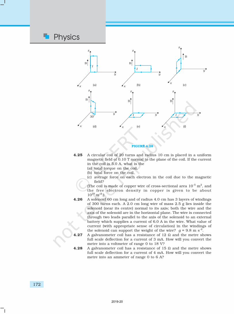
Physics

172

FIGURE 4.28

4.25 A circular coil of 20 turns and radius 10 cm is placed in a uniformmagnetic field of 0.10 T normal to the plane of the coil. If the currentin the coil is 5.0 A, what is the

(a) total torque on the coil,(b) total force on the coil,(c) average force on each electron in the coil due to the magnetic

field?(The coil is made of copper wire of cross-sectional area 10–5 m2, andthe free electron density in copper is given to be about

1029 m–3.)4.26 A solenoid 60 cm long and of radius 4.0 cm has 3 layers of windings

of 300 turns each. A 2.0 cm long wire of mass 2.5 g lies inside the

solenoid (near its centre) normal to its axis; both the wire and theaxis of the solenoid are in the horizontal plane. The wire is connectedthrough two leads parallel to the axis of the solenoid to an external

battery which supplies a current of 6.0 A in the wire. What value ofcurrent (with appropriate sense of circulation) in the windings ofthe solenoid can support the weight of the wire? g = 9.8 m s–2.

4.27 A galvanometer coil has a resistance of 12 Ω and the metre showsfull scale deflection for a current of 3 mA. How will you convert themetre into a voltmeter of range 0 to 18 V?

4.28 A galvanometer coil has a resistance of 15 Ω and the metre showsfull scale deflection for a current of 4 mA. How will you convert themetre into an ammeter of range 0 to 6 A?

2019-20