Chapter 9 Application of PDEs - San Jose State …...9.3.2 Laplace transform method for soluti on of partial differential equations (p.288): We have learned to use Laplace transform

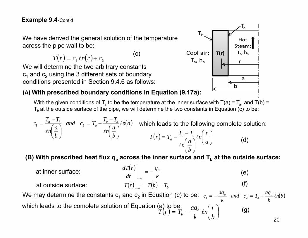
Chapter 9

Application of Partial Differential Equations in Mechanical Engineering Analysis

(Chapter 9 application of PDEs)© Tai-Ran Hsu

* Based on the book of “Applied Engineering Analysis”, by Tai-Ran Hsu, published byJohn Wiley & Sons, 2018 (ISBN 9781119071204)

Applied Engineering Analysis- slides for class teaching*

1

Chapter Learning Objectives

● Learn the physical meaning of partial derivatives of functions.

● Learn that there are different order of partial derivatives describing the rate of changes of functions representing real physical quantities.

● Learn the two commonly used technique for solving partial differential equations by (1) Integral transform methods that include the Laplace transform for physical problems covering half-space, and the Fourier transform method for problems that cover the entire space; (2) the “separation of variable technique.”

● Learn the use of the separation of variable technique to solve partial differential equations relating to heat conduction in solids and vibration of solids in multidimensional systems.

2

9.1 Introduction

A partial differential equation is an equation that involves partial derivatives.

Like ordinary differential equations, Partial differential equations for engineering analysis are derived by engineers based on the physical laws as stipulated in Chapter 7. Partial differential equations can be categorized as “Boundary-value problems” or “Initial-value problems”, or “Initial-boundary value problems”:

(1) The Boundary-value problems are the ones that the complete solution of the partial differential equation is possible with specific boundary conditions.

(2) The Initial-value problems are those partial differential equations for which the complete solution of the equation is possible with specific information at one particular instant (i.e., time point)

Solutions to most these problems require specified both boundary and initial conditions.

3

9.2 Partial Derivatives (p.285):

A partial derivative represents the rate of change of a function involving more than one variable (2 in minimum and 4 in maximum). Many physical phenomena need to be defined by more than one variable as in the following instance:

Example of partial derivatives: The ambient temperatures somewhere in California depend on where and where this temperature is counted. Therefore, the magnitude of the temperature needs to be expressed in mathematical form of T(x,y,z,t), in which the variables x, y and z in the function T indicate the location at which the temperature is measured and the variable t indicates the time of the day or the month of the yaer at which the measurement is taken. The rate of change of the magnitude of the temperature, i.e., the derivatives of the function T(x,y,z,t) needs to be dealt with the change of EACH of all these 4 variables accounted with this function. In other words, we may have all together 4 (not just one) such derivatives to be considered in the analysis. Each of these 4 derivative is called “partial derivative” of the function T(x,y,z,t) because each derivative as we will express mathematically can only represent “part” (not whole) of the derivative for this function that involves multi-variables.

There are two kinds of independent variables in partial derivatives:

(1) “Spatial” variables represented by (x,y,z) in a rectangular coordinate system, or (r,,z) in a cylindrical polar coordinate system, and

(2) The “Temporal” variable represented by time, t.

4

9.2 Partial Derivatives: - Cont’d

Mathematical expressions of partial derivatives (p.286)

xxfxxf

dxxdf

imx

)()()(0

We have learned from Section 2.2.5.2 (p.33) that the derivative for function with only one variable, such as f(x) can be defined mathematically in the following expression, with physical meaning shown in Figure 9.1.:

f(x)

xx x

Tangent line:

f(x)dx

xdf )(

xf

(2.9)

For functions involving with more than one independent variable, e.g. x and t expressed in function f(x,t), we need to express the derivative of this function with BOTH of the independent variables x and t separately, as shown below:

The partial derivative of function f(x,t) with respect to x only may be expressed in a similar way as we did with function f(x) in Equation (2.9), or in the following way:

(9.1)

We notice that we treated the other independent variable t as a “constant” in the above expression for the partial derivative of function f(x,t) with respect to variable x .

Likewise, the derivative of function f(x,t) with respect to the other variable t is expressed as:

ttxfttxf

ttxf

imt

),(),(),(0

(9.2)

5

Figure 9.1

9.2 Partial Derivatives: - Cont’d

Mathematical expressions of higher orders of partial derivatives:Higher order of partial derivatives can be expressed in a similar way as for ordinary functions, such as:

xx

txfx

txxftxf

imx x

),(),(

),(0

2

2

(9.3)

andt

ttxf

tttxf

ttxf

imt

),(),(),(

02

2

(9.4)

There exists another form of second order partial derivatives with cross differentiations with respect to its variables in the form:

xttxf

txtxf

),(),( 22

(9.5)

9.3 Solution Methods for Partial Differential Equations (PDEs) (p.287)

There are a number ways to solve PDEs analytically; Among these are: (1) using integraltransform methods by “transforming one variable to parametric domain after another in theequations that involve partial derivatives with multi-variables. Fourier transform and Laplace transform methods are among these popular methods. The recent available numerical methods such as the finite element method, as will present in Chapter 11 offers muchpractical values in solving problems involving extremely complex geometry and prescribed physical conditions. The latter method appears having replaced much effort required in solving PDEs using classical methods. With readily available digital computers and affordable commercial software such and ANSYS code, this method has been widely accepted by industry. The classical solution methods appears less in demand in engineering analysis as time evolves. 6

9.3 Solution Methods for Partial Differential Equations-Cont’d9.3.1 The separation of variables method (p.287):

The essence of this method is to “separate” the independent variables, such as x, y, z, and t involved in the functions and partial derivatives appeared in the PDEs.

We will illustrate the principle of this solution technique with a function F(x,y,t) in a partial differential equation. The process begins with an assumption of the original function F(x,y,t), to be a product of three functions, each involves only one of the three independent variables, as expressed in Equation (9.6), as shown below:

F(x,y,t) = f1(x)f2(y)f3(t) (9.6)

where f1(x) is a function of variable x onlyf2(y) is a function of variable y only, and f3(t) is a function of variable t only

Equation (9.6) has effectively separated the three independent variables in the original function F(x,y,t) into the product of three separate functions; each consists of only one of the three independent variables.

The 3 separate function f1, f2 and f3 in Equation (9.6) will be obtained by solving 3 individual ordinary differential equations involving “separation constants.” We may than use the methods for solving ordinary differential equations learned in Chapters 7 and 8 to solve these 3 ordinary differential equations.

The partial differential equation that involve the function F(x,y,t) and its partial derivatives can thus be solved by equivalent ordinary differential equations via the separation relationship shown in Equation (9.6) . In general, PDEs with n independent variables can be separated into n ordinary differential equations with (n-1) separation constants. The number of required given conditions for complete solutions of the separated ordinary differential equations is equal to the orders of the separated ordinary differential equations.

7

9.3 Solution Methods for Partial Differential Equations-Cont’d9.3.2 Laplace transform method for solution of partial differential equations (p.288):We have learned to use Laplace transform method to solve ordinary differential equations in Section 6.6, in which the only variable, say “x”, involved with the function in the differential equation y(x) must cover thehalf space of (o<x<∞). Solution of the differential equation y(x) is obtained by converting this equation into an algebraic equation by Laplace transformation with the “transformed expression F(s) in which “s” is the Laplace transform parameter. The solution of the ordinary differential equation y(x) is obtained by inverting the F(s) in its resulting expression. We have also use the Laplace transform method to solve a partialdifferential equation in Example 6.19 (p.194) after having learned how to transform partial derivatives in Section 6.7.

9.3.3 Fourier transform method for solution of partial differential equations (p.288):

Fdxexfxf xi

Fourier transform engineering analysis needs to satisfy the conditions that the variables that are to be transformed by Fourier transform should cover the entire domain of (-∞, ∞). Mathematically, it has the form:

(9.7)

The inverse Fourier transform is:

deFF xi

211 (9.8)

The following Table 9.1 presents a few useful formula for Fourier transforms of a few selected functions. Functions for Fourier Transform f(x) After Fourier Transform F(ω)

(1) f(x-a) F(ω)e-iωa

(2) δ(x)* 1(3) u(x)* (iω)-1

(4)

(5) u(x)sinax

(6) u(x)cosax

0 xe

*δ(x) = Delta function, or impulsive function and u(x) is the unit step function. Both these functions are defined in Section 2.4.2

8

9.3 Solution Methods for Partial Differential Equations-Cont’d

Example 9.2Solve the following partial differential equation using Fourier transform method.

t

txTx

txT

,, 2

2

2

-∞ < x <∞ (9.11)

where the coefficient α is a constant. The equation satisfies the following specified condition: xfxTtxT

t

0,,

0(9.12)

Solution

dxetxTtxTtT xi

,,,*

We will transform variable x in the function T(x,t) in Equation (9.11) using Fourier transform in Equation (9,7):

(a)Apply the above integral to the left-hand-side of Equation (9.11) will yield:

tTdxex

txTx

txT xi ,*,, 22

2

2

2

from Equation (9.10), and

t

tTdxetxTt

dxedt

tTxt

txT xixi

,*,,, 2222 for the right-hand-side of Eq. (9.11)

Equation (9.11) has the form after the transformation:

dt

tdTtT ,*,* 22 (b)

Equation (b) is a first order ordinary differential equation involving the function T*(ω,t) and the method of obtaining the general solution of this equation is available in Chapter 7.

9.3.3 Fourier transform method for solution of partial differential equations:-Cont’d

At this point, we need to transform the specified condition in Equation (9.12) by the Fourier transform defined in Equation (a), or by the following expression:

gdxexfdxexTxTT xixi

0,0,0,* (c)9

9.3 Solution Methods for Partial Differential Equations-Cont’d

Example 9.2- Cont’d

9.3.3 Fourier transform method for solution of partial differential equations:-Cont’d

We will solve the first order ODE in Equation (b) with the solution of T*(ω,t) in Equation (b) and obtain:

t

egtT 2

2

,*

(d)

The solution of the partial differential equation in Equation (9.11) with the specified condition in Equation (9.12) can thus be obtained by inverting the transform T*(ω,t) to T(x,t) using Equation (9.8) by the following expression:

deegdetTtxT xit

xi

2

21,*

21, (e)

where g(ω) is available in Equation (c) to be the Fourier transformed specified condition of T(x,0) in Equation (9.12).

10

9.4 Partial Differential Equations for Heat Conduction in Solids (p.291)

We have learned from Section 7.5 (p.217) that temperature variations in media is induced by heat transmissions. This variation of temperature in media (solids or fluids) is called temperature field.

Heat transfer is a very important branch of mechanical and aerospace engineering analyses because many machines and devices in both these engineering disciplines are vulnerable to heat. According to statistics, over 60% of electronics devices in the US Airforce failed to functions due to excessive heating. Excessive heat flow can also result in a high temperature fields in the structural media, which may result in serious thermal stresses in addition to significant deterioration of material strength and property changes, as presented in Section 7.5.

In this section, we will derive the partial differential equations for heat conduction in solids in both rectangular and cylindrical polar coordinate systems, and solve these equations by using separations of variables technique. Although many of these problems can also be solved by advanced numerical techniques such as finite difference and finite element methods, the classic solutions as will be presented in this chapter, however, will offer engineers with solutions at anywhere in the solid structure, which the numerical methods cannot offer the same. These numerical methods, however, are often used for situations that involve complicated geometry, loading and boundary conditions.

9.4.1 Heat conduction in engineering analysis

11

9.4.2 Derivation of partial differential equations for heat conduction analysis

Heat conduction equation is used to determine the temperature distributions induced byheat conduction in solids, either by heat generation by the solids or by heat from external sources.

This equation will be derived from the law of conservation of energy, in particular, the first law of thermodynamics.

By referring to Figure 9.3 , a solid with a volume is subjected to heat flow in the form of heat flux q(r,t) from external sources to a small element (in the small open circle) in the figure.

The heat leaving the element is q(r+∆r,t) with r designating the spatial variables of (x,y,z) in a rectangular coordinate system or (r,θ,z) in a cylindrical polar coordinate system. Since heat is a form of energy, we may use the law of conservation of energy in the following block diagrams

to derive the mathematical expression for the case:

12

Figure 9.3

9.4.2 Derivation of partial differential equations for heat conduction analysis – Cont’d

We may use the following mathematical expressions to representthe physical quantities in the solid shown in Figure 9.3.

From the block diagram of energy conservation and the above mathematical representations of physical quantities in the block diagram, we may establish the following partial differential equation for the temperature variations in the entire solid to be:

tQtTkt

tTc ,,, rrr

(9.13)

where k = thermal conductivity of the solid material, Q(r,t)= heat generation by the material(such as Ohm heating of Q=iR2 with i being the electric current in Ampere, and R is the electric resistance of the material in Ohms.

13

Figure 9.3

9.4.3 Heat conduction equation in rectangular coordinate system

The general heat conduction equation in Equation (9.13) will take the following form with T(r,t) = T(x,y,z,t):

tzyxQzTk

zyTk

yxTk

xtTc zyx ,,,

(9.14a)

in which kx, ky and kz are the thermal conductivities of the solid along the x-, y- and z-coordinates respectively.

9.4.4 Heat conduction equation in cylindrical polar coordinate system:Heat conduction equation in this coordinate system is obtained by expanding Equation (9.8) as follows with T(r,t) = T(r,θ,z,t):

tzrQzTk

zTk

rrTk

rrTk

rtTc zrr ,,,11

2

(9.14b)

where kr,kθ and kz are thermal conductivities of the material along the r-, θ- and z-coordinate respectively.

14

9.4.5 General heat conduction equation (p.293):

Thermal conductivities kx, ky and kz in Equation (9.14a) and kr, kθ and kz in Equation (9.14b) are used for heat conduction analysis of solids with their thermophysical properties varying in different directions, such as for fiber filament composites. For most engineering analyses, such variation of thermophysical properties do not exist. Consequently a generalize heat conduction equation may be expressed as follows

t

tTk

tQtT

,1,,2 rrr

(9.15)

where k = thermal conductivity of the material and Q(r,t) is the heat generated by the material per unit volume and time.

The symbol α in Equation (9.15) is “thermal diffusivity” of the material with its value equals

to: ck

, it is often used as a measure on how “fast” heat can flow by conduction in solids.

9.4.6 Initial conditions:Complete solution of heat conduction equation in Equation (9.15) involves determining a number of arbitrary constants according to specific initial and boundary conditions.These conditions are necessary to translate the real physical conditions into mathematical expressions. Initial conditions are required only when dealing with transient heat transfer problems in which temperature field in a solid changes with elapsing time. The common initial condition in a solid can be expressed mathematically as: rrr 00

0,, TTtTt

(9.16)

where the temperature field T0(r) is a specified function of the spatial coordinates r only

In many practical applications, the initial temperature distribution T0(r) in Equation (9.16) can be assigned with a constant value such as room temperature at 20oC for a uniform temperature condition in the solid. 15

9.4.6 Boundary conditions:Specific boundary conditions are required in obtaining complete solutions in heat transfer analyses using the general heat conduction equation in (9.15). Four types of boundary conditions are available for this purposes.as will be presented below.

1) Prescribed surface temperature, Ts(t):This type of boundary condition is used to have the temperature at the surface of the solid structure measured by either attaching thermocouples to the structure surface or by some non-contact methods such as infrared thermal imaging scanning camera. The mathematical expression for this case takes the form:

tTtT ss

rrr, (9.17a)

where rs is the coordinates of the boundary surface where temperature are specified to be Ts(t)

2) Prescribed heat flux boundary condition, qs(t):Many structures have their surfaces exposed to a heat source or a heat sink, in such situations,heat is being supplied to or removed from the solids through its outside surface. The mathematical translation of the heat flux to or from a solid surface can be readily carried out by using the Fourier law of heat conduction defined in Equation (7.25). The mathematical formulation of the heat flux across a solid boundary surface can be expressed as:

k

tqtT s ,, s

rri

rnr

s

(9.17b)

where k is the thermal conductivity of the solid material. The symbol in

is the differentiation along the outward-drawn normal to the boundary surface Si. We may express Equation (9.17b) for the boundaries that are impermeable to heat flow, or a boundary that is thermally insulated as:

0,

srnr

r

tT (9.17c)

16

9.4.6 Boundary conditions – Cont’d:3) Convective boundary conditions:

This type of boundary condition applies when the solidstructure is either in contact with a fluid, or is submergedin fluids, as often happen in reality.

Let us derive the mathematical expressions of the boundary conditionsby referring to the sketch in Figure 9.5.

We first recognize that there is a physical “barrier” that retards free heatflow between the solid surface and its contacted fluid. This barrier isoften recognized as the “boundary layer that can be characterized by a “film resistance that is equal to “1/h” with h being the film coefficient as defined inEquation (7.29) in Section 7.5.5. Physically it means that the temperature ofthe solid surface Ts ≠ the temperature of the surrounding bulk fluid Tf.

The following two (2) mathematical expressions are derived to represent the above physical phenomenon:

fTtThn

tTk

,,s

rr

rr

s

From the fact that no heat is being stored at the interface of the solid and fluid, which leads to the following Equality:

Heat flow in solid = Heat flow in fluid or in the form:

fr

TkhtT

kh

ntT

s

srr

r

rr ,,(9.17d)

The above equation involves heat flows in solids by conduction and heat flows in fluids by convection. It is often referred to be the “mixed boundary conditions.” This expression of boundary condition actually could be used for problems involving prescribed surface temperatures in Equation (9.17a) with h→∞, We may also prove that letting h = 0 in Equation (9.17d) will lead to a thermally insulated boundary condition with qs = 0 in Equation (9.17b). 17

Figure 9.5

Example 9.3 (p.295)

Show the appropriate boundary conditions of a long thick wall pipe containing hot steam flow inside the pipe at a bulk temperature Ts with heat transfer coefficient hs.

The outside wall of the pipe is in contact with cold air at a temperature of Ta and with a heat transfer coefficient ha, as illustrated in Figure 9.6.

SolutionA common but logical hypothesize made in this type of engineering analysis is that heat will flow is primarily along the positive radial direction (r) in a long pipe such as in this example because of the greater temperature gradient cross the pipe wall than that along the length. So, the radial direction is the principal direction of heat flow. Consequently, we will account for two boundary surfaces in this analysis, i.e., at the inner surface with r = a and the outside surface at r=b.

Since heat transfer coefficients of both the steam inside the pipe (hs) and the heat transfer coefficient of the air outside the pipe (ha) are given, we may use Equation (9.17d) to establish the convective boundary conditions at both sides of the pipe wall as follows:

(a) At inner boundary with r = a: ss

ar

s

ar

TkhrT

kh

drrdTk

(b) At the outside boundary with r = b: aa

bra

br

TkhrT

kh

drrdTk

in which k = thermal conductivity of the pipe material18

Figure 9.6

Example 9.4 (p.296)

Find the temperature distribution in a long thick wall pipe with inner and outside radii a and b respectively by using the three types of boundary conditions in Equations (9.17a,b,d). Conditions for establishing the mathematical expressions for these boundary conditions with hot steam inside the pipe and the cool surrounding air outside the pipe are indicated in Figure 9.7.

SolutionWe adopt the same principal as described in the last example that the shorter heat flow path along the radial direction of the pipe enables us to assume the principal temperature variationin the pipe wall is with the radius variable (r). Consequently, we may assume that the temperature function that we desire in this analysis is T(r) only. Thus, by select the relevant terms in the PDE in (9.14b), we will have the relevant differential equation of the form:

(a)

Solution of the differential equation in (a) may be obtained by either using Equation (8.6), or by re-arranging the terms that fit the following form of:

0

drrdTr

drd

from which we get the solution T(r) by integrating Equation (b) twice with respect to variable r,leading to the form:

(b)

012

2

dr

rdTrdr

rTd

21 crncrT (c)where c1 and c2 are two arbitrary constants 19

Figure 9.7

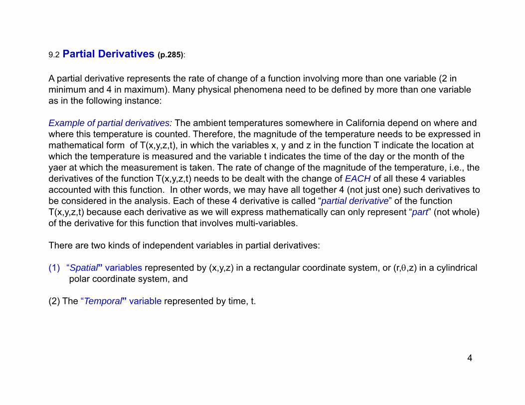
Example 9.4-Cont’d

We have derived the general solution of the temperatureacross the pipe wall to be:

21 crncrT (c)

We will determine the two arbitrary constantsc1 and c2 using the 3 different sets of boundaryconditions presented in Section 9.4.6 as follows:

(A) With prescribed boundary conditions in Equation (9.17a):With the given conditions of:Ta to be the temperature at the inner surface with T(a) = Ta, and T(b) = Tb at the outside surface of the pipe, we will determine the two constants in Equation (c) to be:

an

ban

TTTcand

ban

TTc baa

ba

21 which leads to the following complete solution:

arn

ban

TTTrT baa

(d)

(B) With prescribed heat flux qa across the inner surface and Tb at the outside surface:

kq

drrdT a

ar

(e)at inner surface:

at outside surface: bbrTbTrT

(f)

We may determine the constants c1 and c2 in Equation (c) to be: bnk

aqTcandk

aqc ab

a 21

which leads to the comolete solution of Equation (a) to be:

brn

kaqTrT a

b (g)20

Example 9.4-Cont’d

(c) With mixed boundary conditions in Equation (9.17d):

The 2 appropriate boundary conditions are:

at inner pipe surface: ss

ars

ar

TkhrT

kh

drrdT

(h)

aa

bra

br

TkhrT

kh

drrdT

at outside pipe surface: (j)

Substitute (h) and (j) into Equation (c), we will get:

abnhh

bkh

akh

TThhcas

sa

saas

1

bn

bhk

abnhh

bkh

akh

TThhTca

assa

saasa

2and

The temperature distribution in the pipe wall T(r) may be obtained by substituting the constants c1 and c2 in the above expressions into the solution in Equation (c).

21

9.5 Solution of Partial Differential Equations for Transient Heat Conduction Analysis (p.298)

The partial differential equation presented below and also in in Equation (9.15) is valid for the general case of heat conduction in solids includes transient cases in which the induced temperature field T(r,t) varies with time t.

t

tTk

tQtT

,1,,2 rrr

(9.15)

where r = the position vector and t = time. Q(r,t)= the heat generation by the materialin unit volume and time, k, α = thermal conductivity and thermal diffusivity of the material respectively, with k to be a measure of how well material can conduct heat and the latter α is a measure of how fast the material can conduct heat.

The position vector r may be in rectangular coordinates: (x,y,z) or in cylindrical polar coordinate system (r,θ,z).

The complexity in transient heat conduction analysis is that not only we need to specify the position (r) where the temperature of the solid is accounted for, but we will also need to specify the time t at which the temperature of the solid occurs. We thus need to specify both theboundary and initial conditions such as described in Section 9.4.6 for complete solution of the temperature filed in the solid.

In this section, we will demonstrate how the separation of variables technique described in Section 9.3 will be used to solve this type of problems in both rectangular and cylindrical polar coordinate systems. 22

9.5.1 Transient heat conduction analysis in rectangular coordinate system (p.298)The case that we will present here involves a large flat slab made of a material with thermal conductivity k. The slab has a thickness L as illustrated in Figure 9.8. It has an initial temperature distribution that can be described by a specified function of f(x), and the temperatures of both its faces are maintained at temperature Tf at time t > 0.

We need to determine the temperature variation in the slab with time t, i.e. T(x,t) in the figure after the temperature of both faces of the slab are maintained at Tf.

We may also recognize a fact that the geometry of a large flat slab is a good approximation for the situation of a circular cylinder with large diameter with a large ratio of D/d in which D is the nominal diameter of the hollow cylinder and d is the thickness of the wall of the hollow cylinders. The solution obtained from this analysis of flat slab may thus be used for large hollow cylinders such as pressure vessels of large diameters such as for nuclear reactor vessels in nuclear power plants.

The physical situation of this example is that the flat slab has an initial temperaturevariation through its thickness fits a function T(x.0) = f(x) –a given temperature dis-tribution. Both its surfaces are maintained at a constant temperature Tf at time t >0+

for t > 0. One may imagine that the temperature in the slab will continuously varying with time t, until the temperature in the entire slab reaches a uniform temperature Tf. The purpose of our subsequent analysis, however, is to find the transient temperature T(x,t) in the slab before it reaches the ultimate uniform temperature of Tf.

23

t

txTx

txT

,1,

2

2

The governing differential equation for the aforementioned physical situation may be deduced from heat conduction equations in Equations (9.14a) and (9.15) with the thermal conductivity of the slab material kx = ky = kz=k for being an isotropic material. The term Q(x,y,z,t) in Equation (9.14a) and Q(r,t) in Equation (9.15) are deleted because the slab does not generate heat by itself. Consequently, the equation that matches the the present physical situation becomes:

9.5.1 Transient heat conduction analysis in rectangular coordinate system –Cont’d (p.299)

(9.18)

With the initial condition (IC): xfxTtxT

t

0,,

0

(9.19a)

and the following boundary conditions (BC): 0,0,

0

tTtTtxT fx

0,,

tTtLTtxT fLx

(9.19b)

(9.19c)

We may solve the partial differential equation in Equation (9.18) by using Laplace transform method described in Section 6.5.2 (p. 180) or 9.3 (p.287) by transforming the variable “t” to parametric domain , or use the separation of variables technique as described in Section 9.3.1. However, we may circumvent our effort in the solution of Equation (9.18) by using the separation of variables method with converting the non-homogeneous BCs in Equation (9.19b,c) to homogeneous BCs by the following substitution of u(x,t) to T(x,t):

u(x,t) = T(x,t) ‐ Tf (9.20)24

9.5.1 Transient heat conduction analysis in rectangular coordinate system –Cont’d

0,,,00

fffxx

TTTtxTtoutxu

0,,, fffLxLx

TTTtxTtLutxu

(b)

(c)

The above relation in Equation (9.20) will result in the revised PDEs in Equation (9.18)into the following form:

t

txux

txu

,1,

2

2

(9.21)

with the revised initial condition: ft

Txfxutxu

0,,0 (a)

and the 2 converted boundary conditions:

We are now ready to solve the equation in (9.21) and the associate initial and boundary conditions in Equations (a,b,c) using the separation of variables method as presented below:We will proceed by letting:

u(x,t) = X(x)τ(t) (9.22)

Substituting the relationship in Equation (9.22) into Equation (9.21) will lead to the following expressions:

leads to: and this equality

in which the partialcan now be expressed in ordinary derivatives.

25

derivatives on either sides are obtained.


The expression that we just derived, as shown below

can be expressed in a slight different form after re-arranging the terms to another equality:

The above expression shows a very interesting but unique feature:

The LHS of the above expression involves the variable x only =The RHS of the same expression involves the variable t only

The ONLY condition such an equality can exist is to have both sides of the expressionto equal a CONSTANT!! (we may prove that the constant must be a NEGATIVE constant).

Consequently, we may have the following valid equality:

dttd

tdxxXd

xX

111

2

2

(9.23)

where β is the “separation constant” and it can be either positive or negative constant.

022

2

xXdx

xXd

02 tdt

td

(9.24)

(9.25)

Equation (9.23) results in the following 2 separate ordinary differential equations:

2

2

2 111

dt

tdtdx

xXdxX

26


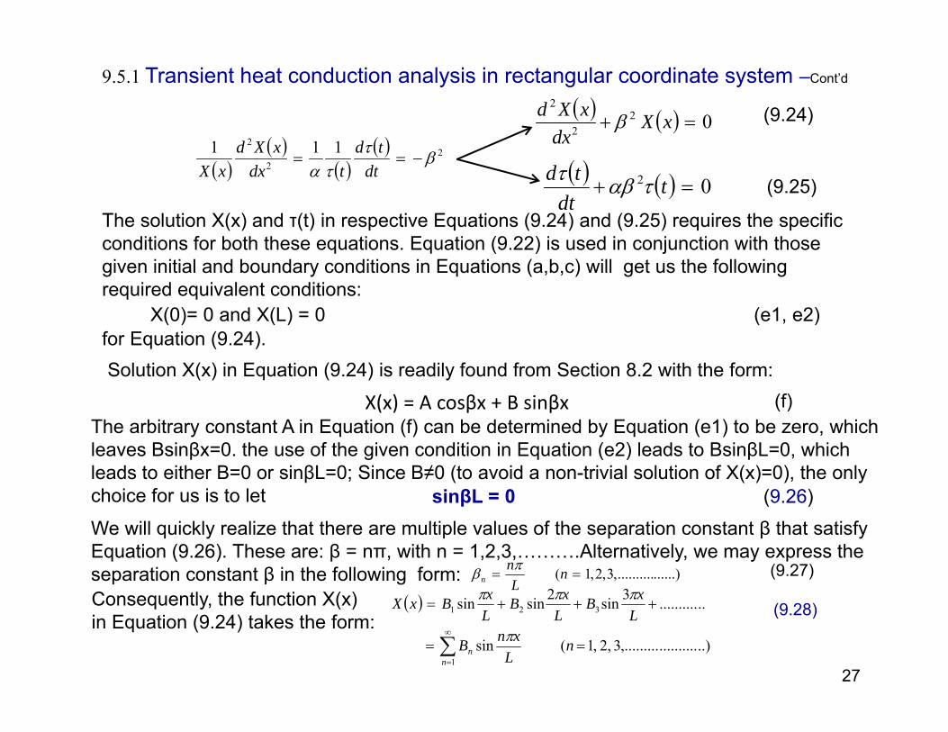
The solution X(x) and τ(t) in respective Equations (9.24) and (9.25) requires the specific conditions for both these equations. Equation (9.22) is used in conjunction with those given initial and boundary conditions in Equations (a,b,c) will get us the following required equivalent conditions:

022

2

xXdx

xXd

02 tdt

td

(9.24)

(9.25)

X(0)= 0 and X(L) = 0 (e1, e2)for Equation (9.24).Solution X(x) in Equation (9.24) is readily found from Section 8.2 with the form:

X(x) = A cosβx + B sinβx (f)The arbitrary constant A in Equation (f) can be determined by Equation (e1) to be zero, whichleaves Bsinβx=0. the use of the given condition in Equation (e2) leads to BsinβL=0, whichleads to either B=0 or sinβL=0; Since B≠0 (to avoid a non-trivial solution of X(x)=0), the only choice for us is to let sinβL = 0 (9.26)

2

2

2 111

dt

tdtdx

xXdxX

We will quickly realize that there are multiple values of the separation constant β that satisfy Equation (9.26). These are: β = nπ, with n = 1,2,3,……….Alternatively, we may express the separation constant β in the following form: ......)..........,3,2,1( n

Ln

n (9.27)

..)..........,.........3,2,1(sin

............3sin2sinsin

1

321

nL

xnB

LxB

LxB

LxBxX

nn

Consequently, the function X(x) in Equation (9.24) takes the form:

(9.28)

27


02 tdt

td (9.25)

Solution of this first order differential equation is: t

nneCt2 (9.29)

where Cn with n = 1, 2, 3,……are multi-valued integration constants corresponding to the multivalued βn in the solution.

L

xnebL

xneBCtxun

tn

t

nnn

nb sinsin,

11

(9.30)

The multi-valued constant coefficients bn=CnBn in Equation (9.30) may be determined by the last available initial condition in Equation (a) in which u(x,o) = f(x)-Tf. Consequently, we have:

L

xnbTxfxun

nfsin0,

1

(9.31)

where f(x) and Tf are the given initial temperature distribution in the slab and the contacting bulk fluid temperature respectively.

28


Determination of the multi-valued constant coefficients bn in Equation (9.30) on P.302:

We will use the “orthogonality property of integrals of trigonometry functions” for the above task.The two applicable properties are presented below:

nmifpnmif

dxp

xmpxnp

2/0

sinsin0

(9.32)

Following steps are taken in determining the coefficient bn with n = 1,2,3,…., in Equation (9.31):

Step 1: Multiply both side of Equation (9.26) with functionL

xnsin

L

xnL

xnbL

xnbL

xnTxfL

xnn

nn

nf sinsinsinsinsin

11

Step 2: Integrate both sides of Equation (g) with integration limits of (0,L):

(g)

dxL

xnbdxL

xnL

xnbdxTxfL

xnn

L

n

L

nnf

L2

100

10

sinsinsinsin

(h)

Step 3: Make use of the orthogonality of the harmonious functions like sine and cosine with the relationships in Equation (9.32):

2sin

0

LbdxTxfL

xnnf

L leading to:

dxL

xnTxfL

bL

fnsin2

0 (9.33)

We thus have the solution of Equation (9.21) to be: L

xnedxL

xnTxfL

txun

tL

fn

sinsin2,1

0

2

The solution of T(x,t) in Equation (9.18) for the temperature distribution in the slab can thus be obtained by the relationship expressed in Equation (9.20) to take the form:

L

xnedxL

xnTxfL

TtxT t

n

L

ffn

sinsin2,2

10

(9.34)

It will not be hard for us to envisage that T(x,∞)→Tf in Equation (9.34) – a solution in reality.29

9.5.2 Transient heat conduction analysis in cylindrical polar coordinate system (p.303)There are many mechanical engineering equipment having geometry that can be better defined by cylindrical polar coordinates (r,θ,z) such as illustrated in the figure to the right:

Cylinders, pipes, wheels, disks, etc. all fit to this kind of geometry such asshown in Figure 9.9..

It is desirable to know how to handle heat conduction in solids of these geometry.

We will present the case of solving heat conduction problem using the separation variable technique in a solid cylinder with radius a as shown in Figure 9.9.

The cylinder is initially with a given temperature distribution of f(r). It is submerged in a fluid with bulk fluid temperature Tf.at time t+0+.

The situation in real application is like having a hot round solid cylinder initially with a temperature variation from hot center cooling down towards its circumference surface described by function f(r). It is a classical case of “quenching” operation in a metal forming operation.

The surrounding contacting liquid at a cooler temperature Tf is vigorously agitated so that the heattransfer coefficient h of the fluid at the contact surface may be treated as “∞” in Equation (9.17d) on p, 295, leading to the boundary temperature of the solid cylinder to be Tf, as stated in the problem. The temperature field in the solid cylinder may be represented by the function T(r,t), in which r = radial coordinate and t is the time into the heat conduction in the solid.

30

Figure 9.9

9.5.2 Transient heat conduction analysis in cylindrical polar coordinate system – Cont’d (p.303)

The applicable PDE for the current application may be deduced from Equation (9.14b) by dropping the second and other terms in the right-hand-side of that equation, resulting in:

r

trTrr

trTt

trT

,1,,12

2

(9.35)

ck

where is the thermal diffusivity of the cylinder material with ρ and c being the mass density and specific heat of the cylinder material respectively.

We will have the given initial condition: rfrTtrTt

0,,0

(a)

and boundary conditions: 0,,

tTtaTtrT far(b1)

The other “inexplicit” boundary condition for solid cylinders or disks is that the temperature at the center of the cylinder or disk must be a finite value at all times. Conversely this implicit boundary condition for the current case meant to be:

valuefinitetTortTtrTr

,0,0,0

(b2)with the PDE in (9.35) and the initial and boundary conditions specified in Equations (a), (b1)and (b2) as specified above, we may proceed to solve for the transient temperature distribution T(r,t) in Equation (9.35) by using the separation of variables technique similar to what we did in the proceeding Section 9.5.1.

Again, for the same reason as in the previous case, we will first convert the non-homogeneous boundary condition in Equation (b1) to the form of homogeneous condition by letting:

u(r.t) = T(r,t) -Tf(c)

Accordingly, Equation (9.35) and the original initial and boundary conditions will have the forms:

rtru

rrtru

ttru

,1,,1

2

2

(9.36)

00,,0

tforTrfrutru ft

00,,

tfortautruar

(d)

(e)31

with

and

We thus have the PDE: r

trurr

trut

tru

,1,,12

2

(9.36)

with conditions: 00,,0

tforTrfrutru ft(d)

00,,

tfortautruar (e)

Upon substituting the above relation in Equation (9.37) into Equation (9.36) will result in the followingExpressions::

rrR

rt

rrRt

ttrR

orr

trRrr

trRt

trR

2

2

2

2 11

(f)

Equation (f) offers the legitimacy of converting the partial derivatives of R(r) and τ(t) to ordinary derivatives as shown below:

drrdR

rdrrRd

rRdttd

t111

2

2

(g)

We notice that the LHS of Equation (g) involves variable t only whereas the RHS of the same expressioninvolve the other variable r only. The only way that such equality can exist is for both sides in Equation (g) to be equal to a same negative separation constant β. We thus have the following relationship:

22

2 111

drrdR

rdrrRd

rRdttd

t(9.38)

32

(9.37)

9.5.2 Transient heat conduction analysis in cylindrical polar coordinate system – Cont’d

Solution of partial differential equation: r

trurr

trut

tru

,1,,12

2

(9.36)


tforTrfrutru ft(d)

00,,

tfortautruar (e)

02 tdt

td

0222

22 rRr

drrdRr

drrRdr

22

2 111

drrdR

rdrrRd

rRdttd

t

We can thus split Equation (9.38) into the following two separate ordinary differential equations:

(9.39)

(9.40)

The solution of Equation (9.39) is identical to Equation (9.29) in the form:

tn

bect2 (h)

where the constant coefficients cn with n = 1, 2, 3,….. is a multivalued integration constants.

We notice that Equation (9.40) is special case of the Bessel equation in Equation (2.27) on p.56 with order n = 0. Consequently, the solution of Equation (9.40) can be expressed by the Bessel functions given in Equation (2.28) on the same page with n = 0 in the following form:

R(r) = A J0(βr) + B Y0(βr) (9.41)

where the constant coefficients A and B will be determined by the boundary conditions stipulated in Equations (d) and (e).

33



trurr

trut

tru

,1,,12

2

(9.36)


tforTrfrutru ft(d)

00,,

tfortautruar (e)

0222

22 rRr

drrdRr

drrRdr (9.40)

We have solve the differential equation in Equation (9.40) to be the expression given in Equation (9.41):

R(r) = A J0(βr) + B Y0(βr)(9.41)

where A and B are two arbitrary constants to be determined by the two boundary conditions applicable in this case are: R(0) for u(0,t) and thus T(0,t). For the condition R(0), we will have, from Equation (h) in the form: R(0)=AJ0(0)+BYo(0), we realize that J0(0) = 1.0 from Figure 2.45 (p.56), but Yo(0)→-∞ as indicated in the same figure. The latter indicates that R(0), therefore T(0) →-∞ (an unbounded temperature at the center of the solid cylinder, which is obviously not a realistic solution. The only way that we may avoid this unrealistic situation is to let the constant B = 0.Consequently, we have the solution in Equation (h) to take the form: R(r) = A J0(βr)

The boundary condition in Equation (e) will lead to the expression: R(a) =A J0(βa) = 0, which requires either:A = 0, or J0(βa) = 0. Since the coefficient B in Equation (h) is already set to be zero (0), to let A=0 will mean the function R(r)=0, an unacceptable trivial solution for the temperature T(r,t). We are thus left with the only option to have:

J0(βa) = 0 (9.42)

Equation (9.42) offers the values of the separation constant β in Equation (9.38) because J0(x) = 0 is an equation that has multiple roots (see Figure 2.45(a) on p.56 like sin(βL) = 0 in Equation (9.26) on p.301. The roots of the equation J0(βa) = 0 in Equation (9.42) may be found either from the Figure 2.45(a) on p.56, or from math handbooks. 34

(j)



trurr

trut

tru

,1,,12

2

(9.36)


tforTrfrutru ft(d)

00,,

tfortautruar (e)

R(r) = A J0(βr) tn

bect2

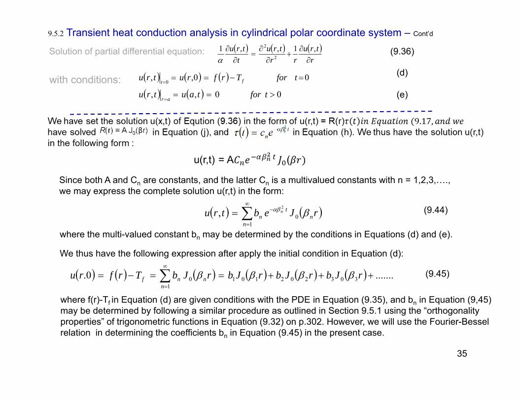
Since both A and Cn are constants, and the latter Cn is a multivalued constants with n = 1,2,3,…., we may express the complete solution u(r,t) in the form:

rJebtru nt

nn

n 0

1

2

,

(9.44)

where the multi-valued constant bn may be determined by the conditions in Equations (d) and (e).

We thus have the following expression after apply the initial condition in Equation (d):

.......0. 30320210101

rJbrJbrJbrJbTrfru nn

nf (9.45)

where f(r)-Tf in Equation (d) are given conditions with the PDE in Equation (9.35), and bn in Equation (9,45) may be determined by following a similar procedure as outlined in Section 9.5.1 using the “orthogonality properties” of trigonometric functions in Equation (9.32) on p.302. However, we will use the Fourier-Bessel relation in determining the coefficients bn in Equation (9.45) in the present case.

35



trurr

trut

tru

,1,,12

2

(9.36)


tforTrfrutru ft(d)

00,,

tfortautruar (e)

The Fourier-Bessel relation has the form (p.307):

aa

nmn

nmnm ifdrrJr

ifdrrJrrJ

00

20

00

0

for different arguments in the Bessel functions in the integral

for same arguments in the Bessel functions in the integral

..........................

...........

303202101302010

302010

rJbrJbrJbrrJrrJrrJ

TrfrrJrrJrrJ f

We will multiply both sides of Equation (9.45) by the following series of Bessel functions: ...........302010 rrJrrJrrJ as shown in the following expression:

and the expansion of both sides of the above expression will result in: ..........30320210100 rJbrJbrJbrrJTrfrrJ nfn (k)

Integrating both sides of Equation (k) with respect to variable r will result in:

........................

........,3,2,1..........

301020100 1

2

0 0

3032021010000

drrJrJrJrJrbdrrJrb

nfordrrJbrJbrJbrrJdrTrfrrJ

aa

nn

n

a

fn

a

(ℓ)

The Fourier-Bessel relation enables us to eliminate the 2nd part of the Bessel functions, and result in:

drrJrbdrTrfrrJa

nnf

a

n

2

0 00 0 (m)

drrJTrfraJa

b n

a

fn

n 002

12

2 We may thus obtain the multi-valued coefficient bn to be: (9.46)

36

9.5.2 Transient heat conduction analysis in cylindrical polar coordinate system – End


trurr

trut

tru

,1,,12

2

(9.36)


tforTrfrutru ft(d)

00,,

tfortautruar (e)

The solution of u(r,t) in Equation (9.36) thus has the form:

rJebtru nt

nn

n 0

1

2

,

(9.44)

where the coefficients bn are obtained fro the integral in Equation (9.46):

drrJTrfraJa

b n

a

fn

n 002

12

2

(9.46)

We may obtain the transient temperature distribution in the cylinder T(r,t) by the relation derived from Equation (c) as: T(r,t) = Ti+u(r,t).

We thus have the solution of the temperature distribution in the cylinder to be:

rJebTtrT nt

nnf

n 0

1

2

,

(9.47)

where the multi-valued coefficients are computed from Equation (9.46)

We notice the appearances of Bessel functions in the solution of this problem. It is normalto see such appearances of Bessel functions in solid geometry involving circular geometry,such as cylinders, disks, and even solids of spherical geometry.

37

9.6 Solution of Partial Differential Equations for Steady-State Heat Conduction AnalysisOften, we are required to find the temperature distributions in solid machine structures with stable heat flow patterns, which makes the temperature distributions in the solids independent of time variation, i.e., the steady state heat conduction. Following are examples on heat flow in the machines in steady-state conditions:

Tubes with finsIC chip with heat spreader:

Jet engine-gas turbine

Tubular heat exchanger:

38

Mathematical representation of multi-dimensional heat conduction in solids is available by using the partial differential equation without the term related to time variable t. The PDE in Equation (9.15) on p.293 is reduced to the following form

9.6 Partial Differential Equations for Steady-State Heat Conduction Analysis (p.308)

02 k

QT rr (9.48)

where the position vector r represents (x,y,z) in rectangular coordinate system, or (r,θ,z) in cylindrical polar coordinate system.

Equation (9.48) is further reduced to the “Laplace equations” in the following form if no heat is generated by the solid:

02 rT (9.49)

We will demonstrate the solution of PDEs for steady-state heat conductions in multi-dimensional solid structure components using separation variables technique in both rectangular and cylindrical polar coordinate systems in the subsequent presentations.

39

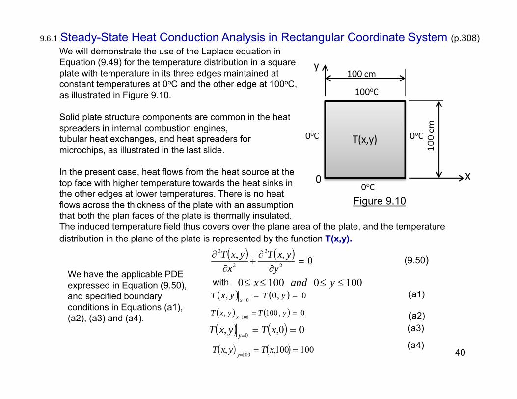
9.6.1 Steady-State Heat Conduction Analysis in Rectangular Coordinate System (p.308)We will demonstrate the use of the Laplace equation in Equation (9.49) for the temperature distribution in a square plate with temperature in its three edges maintained at constant temperatures at 0oC and the other edge at 100oC, as illustrated in Figure 9.10.

Solid plate structure components are common in the heat spreaders in internal combustion engines,tubular heat exchanges, and heat spreaders formicrochips, as illustrated in the last slide.

In the present case, heat flows from the heat source at the top face with higher temperature towards the heat sinks in the other edges at lower temperatures. There is no heat flows across the thickness of the plate with an assumption that both the plan faces of the plate is thermally insulated.The induced temperature field thus covers over the plane area of the plate, and the temperature distribution in the plane of the plate is represented by the function T(x,y).

0,,2

2

2

2

yyxT

xyxT

We have the applicable PDE expressed in Equation (9.50), and specified boundary conditions in Equations (a1),(a2), (a3) and (a4).

10001000 yandx

(9.50)

0,0,0

yTyxTx

0,100,100

yTyxTx

00,,0

xTyxTy

100100,,100

xTyxTy

(a1)

(a2)(a3)

(a4)40

Figure 9.10

with

9.6.1 Steady-State Heat Conduction Analysis in Rectangular Coordinate System – Cont’d

0,,2

2

2

2

yyxT

xyxT

10001000 yandx

(9.50)

0,0,0

yTyxTx

0,100,100

yTyxTx

00,,0

xTyxTy

100100,,100

xTyxTy

(a1)

(a2)(a3)

(a4)

Solution of Partial Differential Equation using Separation of Variables Method (p.309):

Boundary conditions:

There are two variables x and y in the solution of temperature function T(x,y), we will thus let:T(x,y) = X(x) Y(y) (b)

in which function X(x) involves only variable x, and function Y(y) involves variable y only.

Substitute Equation (b) into Equation (9.50), and after re-arranging terms, yields the following expression:

2

2

2

2 11dy

yYdyYdx

xXdxX

We will use the same argument as we did in Sections 9.5.1 and 9.5.2 that the only way the above equality can exist is to have both sides of the equality to be equal to a negative separation constant.

We will thus have the following equality:

22

2

2

2 11 dy

yYdyYdx

xXdxX

(c)

41

9.6.1 Steady-State Heat Conduction Analysis in Rectangular Coordinate System – Cont’dSolution of PDE in Equation (9.50) using Separation of Variables Method-Cont’d:

0,,2

2

2

2

yyxT

xyxT

Equation (c) leads to the split of the PDE in Equation (9.50) into two ordinary differential equations (ODEs) after the separation of the variables x and y as shown below:

022

2

xXdx

xXd

022

2

yYdy

yYd

(d)

(e)

X(0) = 0 X(100) = 0

(f1)

(f2)

Y(0) = 0 (f3)

The original PDE in Equation (9.50):

Both Equations (d) and (e) are homogeneous 2nd order differential equations with the solutions methodsavailable in Section 8.2. We will shown the solutions of these two equations in the following forms:

Solution of Equation (d): xBxAxX sincos (g)

Solution of Equation (e): Y(y) = C coshβy + D sinhβy (k)

We may obtain the expression for the multi-valued separation constant β to be the solution of the characteristic equation of sin(100β) = 0, and the constant coefficient A = 0 upon substitutingThe boundary conditions in Equations (f1) and (f2) into Equation (g). We have thus obtained the multi-valued separation constants βn = (nπ)/L with L=100 and n = 1,2,3,….,n from the roots of the equation sin(100β) = 0. We can thus express the function as:

X(x) = Bnsinβnx (j)

in which Bn with n = 1,2,3,….,n are the multi-valued constant coefficients to be determined later.42

9.6.1 Steady-State Heat Conduction Analysis in Rectangular Coordinate System – Cont’dSolution of Partial Differential Equation (9.50) using Separation of Variables Method-Cont’d:

0,,2

2

2

2

yyxT

xyxT

022

2

xXdx

xXd

022

2

yYdy

yYd

(d)

(e)

X(0) = 0 X(100) = 0

(f1)

(f2)

Y(0) = 0 (f3)

The original partial differential Equation (9.50):

Next, we will solve Equation (e), with a solution (p.310):Y(y) = C coshβy + D sinhβy (k)

The boundary condition in Equation (f3) would make the constant coefficient C = 0. Consequently,we will have the function Y(y) to take the form:

Y(y) = Dnsinhβny with n=1,2,3,…n (m)

We have obtain the solution T(x,y) of Equation (9.50) after substituting the expressions of X(x) in Equation (j) and Y(y) in Equation (m) into Equation (b) and result in:

ynxnb

ynxnDByYxXyxT

nn

nn

nn

100sinh

100sin

100sinh

100sin,

1

11

(n)

43

9.6.1 Steady-State Heat Conduction Analysis in Rectangular Coordinate System – Cont’d

Solution of Partial Differential Equation (9.50) using Separation of Variables Method-Cont’d:

0,,2

2

2

2

yyxT

xyxT

10001000 yandx

(9.50)

0,0,0

yTyxTx

0,100,100

yTyxTx

00,,0

xTyxTy

100100,,100

xTyxTy

(a1)

(a2)(a3)

(a4)

ynxnb

ynxnDByYxXyxT

nn

nn

nn

100sinh

100sin

100sinh

100sin,

1

11

(n)

The unknown coefficients bn in Equation (m) may be determined by using the remaining boundary condition in Equation (a4) that T(x,100) = 100, which leads to:

nxnbxTn

n sinh100

sin100100,1

xnnbn

n 100sinsinh100

1

or (p)

By following the same procedure in in using the orthogonality of trigonometric functions in Section 9.5.1,on p.298, We will determine the constants bn in Equation (p) to be:

......................,3,2,1sinh

1cos200

nwith

nnnbn (q)

Leading to the solution: ynxnnnnyxT

n 100sinh

100sin

sinhcos1200,

1

(9.51)

44

9.6.2 Steady-State Heat Conduction Analysis in Cylindrical Polar Coordinate System (p.311)

We will explore how the separation of variables technique may be used in steady-state heat conduction analysis in cylindrical polar coordinate system by this case illustration.

The case we have here involves a solid cylinder with radius a and length L with temperature at the circumference and the bottom end maintained at 0oC and the temperature at the top surface is subjected to a temperature distribution that fits a specified function F(r) as shown in Figure 9.11.

We realize the physical situation in which heat flows from the top end of the cylinder in boththe radial and longitudinal direction. We may thus designate the temperature in the cylinder by T(r,z) in a cylindrical polar coordinate system.

The governing PDE for T(r,z) in a steady-state heat conduction as described above may be obtained by selecting the right terms in Equation (9.14b) in cylindrical polar coordinate system in the following form:

0,,1,2

2

2

2

z

zrTr

zrTrr

zrT (9.52)

with specified boundary conditions:and

T(a,z) = 0

T(0,z) ≠ ∞

(a1)(a2)

45

Figure 9.11

9.6.2 Steady-State Heat Conduction Analysis in Cylindrical Polar Coordinate System – Cont’d

0,,1,2

2

2

2

z

zrTr

zrTrr

zrT (9.52)

with specified boundary conditions: T(a,z) = 0 T(0,z) ≠ ∞ (a1, a2))(a3)

Solution of the Partial Differential Equation using Separation of Variable Technique:

T(r,0) = 0

Following the usual procedures in separation of variable technique (p.312) , we let:

T(r,z) = R(r) Z(z) (b)

where the functions R(r) and Z(z) involve only one variable r and z respectively.

Upon substituting the above expression in Equation (b) into Equation (9.52), and after re-arranging the terms, we will get the following equality:

2

2

2

2 111z

zZzZr

rRrrRr

rRrR

(c)

The only way that the above equality can exit is having both sides to be equal to a constant:

We thus have:

22

2

2

2 111 dz

zZdzZdr

rdRrrRdr

rRdrR

(d)

0,,1,2

2

2

2

z

zrTr

zrTrr

zrT

We have thus split the PDE in Equation (9.52) into two separate ODEs as follows: 022

2

rRrdr

rdRdr

rRdr

022

2

zZdz

zZd

(e)

(f)

R(a) = 0R(0) ≠ ∞Z(0) = 0

Satisfying the conditions: (g1)(g2)(g3)

46

9.6.2 Steady-State Heat Conduction Analysis in Cylindrical Polar Coordinate System – Cont’d

Solution of the Partial Differential Equation using Separation of Variable Technique-Cont’d:

The solution of the ODE in Equation (e) involves Bessel functions as in the case in Section 9.5.2 and in Equation (9.41) on p.305 to take the form: : rYBrJArR 00

The condition specified condition in Equation (g2) results in having the constant coefficient in the above expression to be: B = 0, because the second term in the above solution in the above expression cannot be allowed in the expression because Y0(0)→-∞, which is not realistic. Hence we have: J0(βna) = 0 (j)

The separation constant β is obtained from Equation (j), and there are multiple roots of that equation, with: β = β1, β2, β3,…...βn with n = 1,2,3,….,n. The solution of other ODE in Equation (f) is:

Z(z) = C cosh(βz) + D sinh(βz) (k)

Substitution of the condition Z(0) = 0 in Equation (a3) into Equation (k) will lead to the constant C = 0. We will thus have: Z(z) = D sinh (βz). However, since Z(z) involve the multi-valued βn, We may express Z(z) in the form: Z(z) = Dn sinh(βnz) (m)

We can thus express the solution T(r,z) in Equation (9.52) in the form of: T(r,z) = [AnJ0(βnr)][Dnsinh(βnz)] with n = 1,2,3,…..n, or in a more compact form:

zrJbzrT bn

nn sinh,1

0

(9.53)

Where bn are multi-valued constant in the the above equation that may be obtained by using the Fourier-Bessel relation as expressed on P. 307, resulting in the following form:

...............,3,2,1

sinh2

0 021

2 nwithdrrrJLLJL

rFb n

L

nnn

(n)

47

9.7 Partial Differential Equations for Transverse Vibration of Cable Structures (p.314)

Transverse vibration of strings (equivalent to long flexible cable structures in reality) are used commonly used in structures such as power transmission lines, guy wires, suspension bridges.

These structures, flexible in nature, are vulnerable to resonant vibrations, which may result indevastations in public safety and property losses to our society.

A cable suspensionBridge at the verge of collapsing:

Long power transmission lines Radio tower supported by guy wires

The world famousGolden GateSuspension Bridge

48

9.7.1 Derivation of partial differential equation for free vibration of cable structures

We begin our derivation of math models for the vibrationanalysis of strings (equivalent to long flexible cables) with an initial sagged shape that can be described by a functionf(x) as illustrated in Figure 9.15.

Figure 9.15 A Long Cable Initially in Statically Equilibrium State

Following idealizations (or hypotheses) were made in the derivation of mathematical modes for free vibration analysis of cable structures:

(1) The cable is as flexible as a string. It means that the cable has no strength to resist bending. Hence we will exclude the bending

moment and shear forces in our subsequent derivations.

(2) There exists a tension in the string in its free-hung static state as shown in Figure 9.15. This tension is so large that the weight, but not the mass, of the cable is neglected in the analysis.

(3) Every small segment of the cable along its length, i.e. the segment with a length x moves in the vertical direction only during vibration.

(4) The vertical movement of the cable along the length is small so the slope of the deflection curve of the cable is small.

(5) The mass of the cable along the length is constant, i.e. the cable is made of same material along its entire length.

49

9.7.1 Derivation of partial differential equation for free vibration of cable structures – Cont’d

A slight instantaneous lateral movement of the cable in Figure 9.15 at time t = 0 will result in laterally vibrateup-and-down in the x-y plane as shown in Figure 9.16(a)

(a) Instantaneous shape at time t (b) Forces on a segment (Detail A)

Figure 9.16 Shape of a vibrating Cable

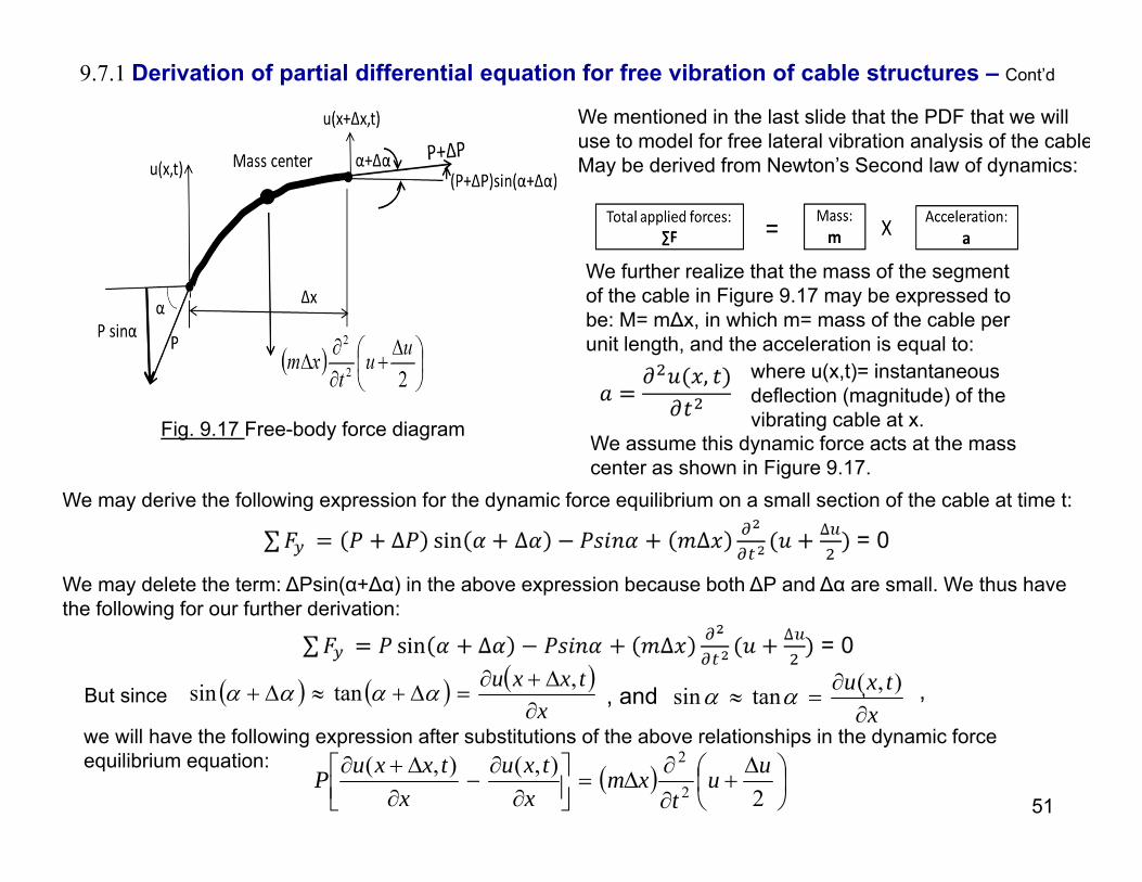
Figure 9.17 Free-body Force diagram of a vibrating cable

Let the mass per unit length of the string be designated by m. The total mass of string in an incremental length x in Figure 9.16 (b) and 9.17 will thus be (mx). The condition for a dynamic equilibrium at time t as illustrated in Figure 9.17 according to Newton’s second law presented in the equation of motion has the following relationship:

50


Fig. 9.17 Free-body force diagram

We mentioned in the last slide that the PDF that we will use to model for free lateral vibration analysis of the cableMay be derived from Newton’s Second law of dynamics:

We further realize that the mass of the segment of the cable in Figure 9.17 may be expressed tobe: M= m∆x, in which m= mass of the cable perunit length, and the acceleration is equal to:

where u(x,t)= instantaneousdeflection (magnitude) of the vibrating cable at x.

We assume this dynamic force acts at the mass center as shown in Figure 9.17.

We may derive the following expression for the dynamic force equilibrium on a small section of the cable at time t:

We may delete the term: ∆Psin(α+∆α) in the above expression because both ∆P and ∆α are small. We thus have the following for our further derivation:

x

txxu

,tansin

xtxu

),(tansin But since ,

we will have the following expression after substitutions of the above relationships in the dynamic force equilibrium equation:

, and

2),(),(

2

2 uut

xmx

txux

txxuP51

,


2),(),(

2

2 uut

xmx

txux

txxuP

If we divide every term in the last expression we will obtain the following expression:

2

),(),(

2

2 uut

mx

xtxu

xtxxu

P

By imposing the condition that the function of the lateral deflection u(x,t) of the vibrating cable varies(changes) its magnitudes continuously along the cable length in the x-coordinate, i.e. ∆x→0, and theincrement of u(x,t), i.e. ∆u is small enough to be neglected (i.e. ∆u→0), the above expression may beexpressed in the following form:

2

2

0

),(),(),(

xtxu

xx

txux

txxu

imx

or

2

),(2

2

2

2 uut

mx

txuP

We thus have the PDE for the free vibration analysis of long flexible cable in the form of:

2

22

2

2 ),(),(x

txuat

txu

(9.54)

where mPa with P = tension in the string with a unit of Newton (N) and m = mass of

the cable per unit length in kg/m. The unit for the constant a in Equation (9.54) is thus m/s.

52

or

9.7.2 Solution of PDE for free vibration analysis of cable structures (p.318)

We will demonstrate the application of Equation (9.54) for the free vibration analysis of a long cable structure illustrated in Figure 9.18.

The cable initially has the shape in the dotted curve in Figure 9.18 that can be described by function f(x).

Lateral vibration of the cable with instantaneous magnitudes u(x,t)is induced to the cable by a small instantaneous disturbance with a slight vertical push to the cable downwardthat produces the instantaneous shape of the cable as shown in the sloid curve in the same figure at time t.

The free vibration of the cable with the lateral amplitudes u(x,t) is sustained by the “mass” of the cable materialand its inherit “elasticity” of the cable. Our analysis is to solve u(x,t) for the physical situation described above.

We will use Equation (9.54) to solve for the u(x,t) by the separation of variables technique, as we did in Section 9.6 for heat conduction analysis. We will thus have the following mathematical model for the solution:

2

22

2

2 ),(),(x

txuat

txu

The PDE: (9.54)

The initial conditions: xfxutxut

0,,0

00,,

0

xut

txu

t

The end (boundary) conditions: 0,0,0

tutxux

0,,

tLutxuLx

(9.55a)

(9.55b)

(9.56a)

(9.56b)53

Figure 9.18

9.7.2 Solution of partial differential equation for free vibration analysis of cable structures – Cont’d

2

22

2

2 ),(),(x

txuat

txu

The partial differential equation: (9.54)

The initial conditions: xfxutxut

0,,0

00,,

0

xut

txu

t

The end (boundary) conditions: 0,0,0

tutxux

0,,

tLutxuLx

(9.55a)

(9.55b)

(9.56a)

(9.56b)

Solution of Partial Differential Equation (9.54) by Separation of Variables Method (p.319):

We will need to separate these two variables x and t from the function u(x,t) in Equation (9.54) by letting: u(x,t) = X(x) T(t) (9.57)

The relation in Eq. (9.57) leads to:

xXtTxxXtTtTxX

xxtxu '(,

tTxXttTxXtTxX

tttx ',

and

xXtTx

txuxx

txu ",,2

2

xXtTt

txutt

txu ",,2

2

and

Substituting the above expressions into Equation (9.54) will lead to:

2

2

2

2

2

)()(

1)()(

1dx

xXdxXdt

tTdtTa

LHS = = RHS = a constant (-β2)

22

2

2

2

2

)()(

1)()(

1 dx

xXdxXdt

tTdtTa

(9.58)We thus have:54

22

2

2

2

2

)()(

1)()(

1 dx

xXdxXdt

tTdtTa

We will thus get two ordinary differential equations from (9.58):

0)()( 222

2

tTadt

tTd

0)()( 22

2

xXdx

xXd

(9.59)

(9.61)

After applying the same separation of variables as illustrated in Eq. (9.57) on the specified conditions in Equations (9.55) and (9.56), we get the two sets of ODEs with specific conditions in the following expressions:

0)()( 222

2

tTadt

tTd 0)()( 22

2

xXdx

xXd (9.59) (9.61)

T(0) = f(x) (9.60a)

0)(

0

tdt

tdT (9.60b)

X(0) = 0

X(L) = 0

(9.62a)

(9.62b)

Both Equations (9.59) and (9.61) are linear 2nd order ODEs with their solutions to be in the following forms:T(t) = A Sin(βat) + B Cos(βat) (9.63) X(x) = C Sin(βx) + D Cos(βx) (9.64)


55


u(x,t) = [A Sin(βat) + B Cos(βat)][ C Sin(βx) + D Cos(βx)]

T(t) = A Sin(βat) + B Cos(βat) X(x) = C Sin(βx) + D Cos(βx)

where A, B, C, and D are arbitrary constants need to be determined from the given initial andboundary conditions given in Eqs. (9.60a,b) and (9.62a,b)

From Eq. (9.62a): X(0) = 0:

Determination of arbitrary constants:Let us start with the solution: X(x) = C Sin(βx) + D Cos(βx) in Eq. (9.64):

C Sin (β*0) + D Cos (β*0) = 0, which means that D = 0 X(x) = C Sin(βx)

Now, from Eq. (9.62b): X(L) = 0: X(L) = 0 = C Sin(βL)

At this point, we have the choices of letting C = 0, or Sin (βL) = 0 from the above relationship. A careful look at these choices will conclude that C ≠ 0 (why?), we thus have:

Sin (βL) = 0The above expression is a transcendental equation with an infinite number of roots for the solutions with βL= 0, π, 2π, 3π, 4π, 5π…………nπ , in which n is an integer number. We may thus obtain the values of the “separation constant, β” to be:

..)..........4,3,2,1,0( nL

nn

(9.66) 56

The lateral amplitude of vibration cable u(x,t) in Figure 9.18 or the solution of Equation (9.54) can thus be expressed by sustituting the expressions in Equations (9.63) and (9.64) in Equation (9.57) to give:

u(x,t) = [A Sin(βat) + B Cos(βat)][ C Sin(βx) + D Cos(βx)]

Now, if we substitute the solution of X(x) in Eq. (9.64) with D=0 and βn = nπ/L with n = 1, 2, 3,..into the solution of u(x,t) expressed in the following form:

We will get:

( , ) n n nu x t ASin at BCos at C Sin xL L L

(n = 1, 2, 3,,……..)

By combining constants A, B and C in the above expression, we have the interim solution ofu(x,t) to be:

xL

nSinatL

nCosbatL

nSinatxu nn

),( (n = 1, 2, 3,,……..)

We are now ready to use the two initial conditions in Eqs (9.55.a) and (9.55b) to determine constants an and bn in the above expression:

Let us first look at the condition in Eq. (9.55b): 0),(

0

tttxu

0 0

( , ) 0n n

t t

u x t n a n at n at nCos Sin Sin xt L L L La b

But since 0nSin xL

(why?) an = 0

1( , )

nn

n a n au x t Cos t Sin xL Lb

Thus, the only remaining constants to be determined are: bn in the above expression.


57

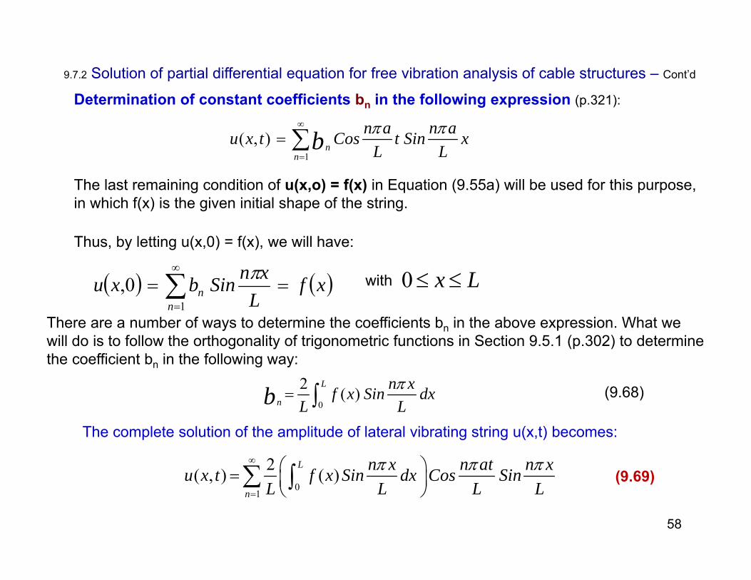
Determination of constant coefficients bn in the following expression (p.321):

1

( , )n

n

n a n au x t Cos t Sin xL Lb

The last remaining condition of u(x,o) = f(x) in Equation (9.55a) will be used for this purpose, in which f(x) is the given initial shape of the string.

There are a number of ways to determine the coefficients bn in the above expression. What we will do is to follow the orthogonality of trigonometric functions in Section 9.5.1 (p.302) to determine the coefficient bn in the following way:

Thus, by letting u(x,0) = f(x), we will have:

xfL

xnSinbxun

n

1

0, Lx 0with

0

2 ( )L

n

n xf x Sin dxL Lb

(9.68)

The complete solution of the amplitude of lateral vibrating string u(x,t) becomes:

01

2( , ) ( )L

n

n x n at n xu x t f x Sin dx Cos SinL L L L

(9.69)


58

9.7.3 Convergence of Series Solutions (p.322)

Solution to partial differential equations by the separation of variables technique such as presented in Sections 9.5 to 9.7 include summations of infinite number of terms associated with the infinite number of roots of transcendental equation (or characteristic equations as mentioned in Chapter 4.The solution in Equation (9.69) for the PDE in Equation (9.54) is also in the form of infinite series.

Numerical solutions of these equations can be obtained by summing up the solutions with each assigned value of n, that is with n = 1, 2, 3, …….to a very large integer number.

In normal circumstances, these infinite series solutions should converge fairly rapidly, so one needs only to sum up approximately a dozen terms with the number n up to 12 for reasonably accurate solutions of the problems.. However, the effect of the convergences of infinite series, such as the one in Equation (9.69) on the accuracy of the analytical results remains a concern to engineers in their analyses.

We will demonstrate the convergence of a series solution related to Equation (9.69) for the vibration of a long cable similar to the situation depicted in Figure 9.18 with L = 20 m and the constant coefficient a = 120 m/s. We assume that the initial shape of the cable can be described by a function x

Lxf sin25.0

1

20

0 20sin

4sin6cos

4011,5

nxdxnnnu

The magnitude of the amplitude of vibrating cable at x = 5 m at t = 1 second is from Equation (9.69) is of the form:

or in the form with numerical values of n = 1,2,3,….,n:u(5,1) = u1 + u2 + u3 + u4 + u5 +………………………..+ un 59

9.7.3 Convergence of Series Solutions – Cont’d

u1 u2 u3 u4 u5 u6 u7 u8 u9 u10 u11 u12 u13 u14 u15 u161.6E-2

3.8E-2

2.8E-2

0 -9.38E-3

3.22E-3

9.38E-3

0 -5.63E-3

1.14E-3

5.63E-3

0 -4.02E-3

5.77E-4

4.02E-3

0

We used the MicroSoft Excel software to compute the numerical values of u(5,1) with n = 1,2,3,…,16 with the computed results shown in the following Table:

and with more terms with additional values of n (up n = 30) in Figure 9.19:

5 10 15 20 25 30

0.04

0.02

0.02

0.04

u n

n

Figure 9.19 Convergence of infinite series solution of Equation (9.69) at x = 5, t=1

We observed from this particular case of numerical solutions of the infinite series solution of Equation (9,69) that inclusion of the first 20 terms in the series (i.e., n = 1,2,3,…..,20) would offer reasonably accurate solution of u(5,1) because of the continuous diminishing of the effects of the values of u(5,1) with the inclusion of terms with additional terms withn-values, as illustrated in this figure.

60

9.7.4 Modes of Vibration of Cable Structures (p.323)

x

X = 0

X

L

Shape @ t = 0: f(x)InstantaneousDisplacement @ x and time t: u(x,t)

Vibration after t = 0+

Initial shape

We have just derived the solution on the AMPLITUDES of vibrating cables, u(x,t) to be:

01

2( , ) ( )L

n

n x n at n xu x t f x Sin dx Cos SinL L L L

(9.69)

We realize from the above expression that the solution consists of INFINITE number of termswith n = 1, n = 2, n = 3,……… What it means is that each term alone in the infinite series in Equation (9.69) is a VALID solution. Hence: u(x,t) with one term with n = 1 only is one possible solution, and u(x,t) with n = 2 only is another possible solution, and so on and so forth.

Consequently, because the solution u(x,t) also represents the INSTANTANEOUS SHAPEof the vibrating string, there could be many POSSIBLE instantaneous shape of the vibrating string depending on what the terms in Eq. (9.69) are used.

Predicting the possible forms (or INSTATANEOUS SHAPES) of a vibrating string is calledMODAL ANALYSIS 61

The First Three Modes of Vibrating Cables:We will use the solution in Eq, (9.69) to derive the first three modes of a vibrating string.

Mode 1 with n = 1 in Eq. (9.69):

1 1( , ) at nx t Cos Sin x

L Lu b

The SHAPE of the Mode 1 vibrating string can be illustrated according to Eq, (91.71a) as:

We observe that the maximum amplitudes of vibration occur at the mid-span of the string,As illustrated in Figure 9.20.The corresponding frequency of vibration is obtained from the coefficient in the argumentof the cosine function with time t in Equation (9.69), i.e.:

(9.70)

where P = tension in Newton or pounds, and m = mass density of string/unit lengthin kg/m3 or slugs/in.

9.7.4 Modes of Vibration of Cable Structures – Cont’d

(9.69)

mP

LLaLaf

21

22/

1

62

Figure 9.20

9.7.4 Modes of Vibration of Cable Structures – Cont’d

Mode 2 with n = 2 in Eq. (9.69):we will have the amplitude of the vibrating cable to be:

2 2

2 2( , ) ax t Cos t Sin xL Lu b

(9.71a)

Possible shape of thecable in Mode 2 vibration:

Mode 3 with n = 3 in Eq. (9.69):mP

LLaLaf 1

2/2

2

Frequency of Mode 2 vibration: (9.72)

3 3

3 3( , ) ax t Cos t Sin xL Lu b

(9.73a)

Possible shape of theCable in Mode 3 vibration:

mP

LLaLaf

23

23

2/3

3

Frequency of Mode 3 vibration: (9.74)

63

Modal analysis provides engineers with critical information on where the possible maximum amplitudes may exist when the string vibrates, and the corresponding frequency of occurrence.

Identification of locations of maximum amplitude allows engineers to predict possible locations of structural failure, and thus the vulnerable location of string (long cable) structures.

Of course, the multiple number of natural frequencies fn such as indicated in the Equations (9.70), (9.72) and (9.74) for the cable in Figure 9.18 with Mode number n =1,2,3, are the indicators of what the frequencies of the applied intermittent loads should be avoided to this kind of structures in order to avoid the devastating resonant vibration of the structure. Modal analysis of cable structures such as illustrated in Figures 9.12-9.14 is thus a critically important part of the analysis.

Physical Importance of Modal Analysis in Vibration of Cable Structures

64

Example 9.6 – A numerical case illustration of vibration analysis of a cable structure (p.325).

A flexible cable 10 m long is fixed at both ends with a tension of 500 N in the free-hung state (see the figure in the right.

The cable has a diameter of 1 cm and with a mass density ρ = 2.7 g/cm3.

If the cable begins to vibrate by an instantaneous but small disturbance from its initial shape that can be described by the function f(x) = 0.005x(1-x/10). Determine the following:

a) The applicable differential equation for the amplitudes of vibration of the cable represented by u(x,t) in meters, in which t is the time into the vibration with a unit of second (s),

b) The mathematical expressions of the applicable initial and end conditionsc) The solution of u(x,t) of the differential equation in metersd) The solution of amplitude of the vibrating cable in Mode 1, i.e., u1(x,t) with the

magnitude and location of the maximum deflection of the cable in this mode of vibration.

e) The numerical values of the frequencies of the first and second mode of vibrationf) The physical significance of these mode shapes.

65

Example 9.6 – A numerical case illustration of vibration analysis of a cable structure-Cont’d.

Solution (p.326):

We realize the following specific conditions:

The length of the cable L = 10 m, with a diameter d = 1 cm = 0.01 mThe cable is made of aluminum with a mass density ρ = 2.7 g/cm3

The cable is subjected to a tension P = 500 N and with initial sag described by the function f(x):

101005.0 xxxf

a) The applicable differential equation for the amplitudes of vibration is Equation (9.54)

2

22

2

2 ),(),(x

txuat

txu

(9.54)

mPa in which P = tension in the cable = 500 N and m = mass per unit length which

needs to be computed with given conditions. The mass per unit length of the cable is m = M/L where M = total mass of the cable with M = ρV with V being the volume of the cable.

We will get the volume of the cable be computed by the expression 342

1085.74

mxLdV

We will thus have the total mass of the cable M = ρV = (2.7x103)(7.85x10-4) = 2.12 kg, leading to the mass per unit length of the cable to be 0.212 kg/m. The constant coefficient according to the expression in Equation (9.54) is:

smmPa /56.48

212.0500

The applicable PDE in equation (9.54) thus takes the form:

(a)

66

with the constant coefficient a in the above equation determined by the following expression:

Example 9.6 – A numerical case illustration of vibration analysis of a cable structure-Cont’d.

b) The mathematical expressions of given initial and end conditions:Solution – Cont’d (p.326)

The initial conditions:

101005.00,,

0

xxxfxutxut

(b1)

00,,

0

xut

txu

t

(b2)The end conditions:

0,0,0

tutxux

0),10(,,

tutLutxuLx

(c1)

(c2)

c) The solution of u(x,t) of Equation (a) satisfying the given conditions in Equations (b1, b2) and Equations (c1 and c2) will be obtained as follows:

The solution of Equation (a) is similar to that of Equation (9.69) with a = 48.56 m/s in the following expression:

xntndxxnxxtxun 10

sin10

56.48cos10

sin10

1005.0102,

10

01

nxntdxxnxxtxun

314.0sin25.15cos10

sin10

1005.051,

10

01

or (d)

nxntn

nn

txun

314.0sin25.15cos2111.0, 33

22

1

(e)or

67

Example 9.6 – A numerical case illustration of vibration analysis of a cable structure-Cont’d. Solution – Cont’d (p.322)

d) The amplitude of the vibrating cable in Mode 1, i.e., u1(x,t) with the magnitude and location of the maximum deflection of the cable in this mode of vibration:The required solution is obtained by letting n = 1 in Equation (e) as:

xtxttxu 314.0sin25.15cos02376.0314.0sin25.15cos2111.0, 31

(f)

The maximum amplitude occurs at the mid-span of the cable at x = 5 m, and at the time when cos15.25t = 1.0. We thus have the maximum amplitude u1,max = 0.02376 m, or 2.376 cm at x = 5 m and at time 15.25t = π, or time t = π/15.25 = 0.2 s.

e) The numerical values of the frequencies of the first and second mode of vibration:We may use Equations (9.70) and (9.72) to compute the numerical values of the frequencies of the first and second mode of vibration as follows:

Hzxm

PL

f 43.2212.0

5001021

21

1 HzmP

Lf 86.4

212.0500

1011

2 for Mode 1, and for Mode 2

f) The physical significance of these mode shapes to the design engineerEngineers will use the outcomes of the above modal analysis to advise the users of this cablestructure on possibility of devastating resonant vibration of the cable structure should the frequency of applied cyclic force, such as wind force coincides any of the natural frequencies computed in Part (e) in the solutions. The users will also be made aware of the locations where maximum amplitudes of vibration may occur as the mode shapes indicate in the modal analysis. They should avoid placing delicate attachments to these locations on the cable structure to avoid potential damages due to excessive vibration at these locations.

68

9.8 Partial Differential Equations for Transverse Vibration of Membranes (p.328)

Solids of plane geometry, such as thin plates are common appearance in machines and structures. Thin plates (or thin diaphragms) can be as small as printed electric circuit boards with micrometers in size or as large as floors in building structures. Like flexible cables, thin flexible plates are normally flexible and be vulnerable to transverse vibration. In some cases, these plates may rupture due to resonant vibrations, resulting in significant loss of property, and even human lives.

This section will derive appropriate PDEs that allow engineers to assess the amplitudes in free vibration of thin plates that are flexible enough to be simulated to thin membranes. Engineers may use this mathematical model for their modal analysis for the safe design of these types of machine components and structures.

69

9.8.1 Derivation of partial differential equation for plate vibrations (p.328)

We will derive the mathematical model for the transverse vibration of thin plates with the following idealizations and hypotheses:1) The derivation of mathematical expressions is based

on the lateral (vertical) displacement of solids of plane geometry that are flexible and offer no resistance to bending. In reality, the structure fits the description of “membranes“ in the subsequent analysis.

4) The thin plate is initially flat with its edges fixed. There is an initial sag represented by a function f(x,y) sustained by in-plane tension P per unit length of the plate in all directions. The tension P is large enough to justify neglecting the weight of the plate.

5) Figure 9.23 defines the plate in the (x,y) plane with lateral displacement z(x,y,t), the amplitude of vibration of the plate at the locations defined by the x-y coordinates and at time t.

6) Every part of the plate vibrates in the direction perpendicular to the plane surface of the plate, i.e., in the z-coordinate as illustrated in Figure 9.24 The slopes of the deformed surface of the plate at all edges are small.

7) The mass per unit area of the plate, designated by the symbol (m) is uniform throughout the plate.

2)Thin plates with unsupported large plane areas that are sufficiently flexible in lateral deformations.

3) Being flexible, there is no shear stress in the deformed thin plates.

Figure 9.23 Transverse vibration of thin plate

We notice that the solution of the amplitudes of vibrating membrane (or thin plate) z(x,y,t) now involves 3 independent variables: x,y and t. We may well image that it would be a much more complicated analysis problem than the cases that we have covered so far in this book.

70

9.8.1 Derivation of partial differential equation for plate vibrations – cont’d (p.329)

Figure 9.24 A free-body diagramof forces in an element of vibrating membraneat time t

Figure 9.24 is a free-body diagram which shows all forces acting on a small deformed element of the plate during a lateral vibration. The situation satisfies a dynamic equilibrium condition with the summation of all forces present at time t be equal to zero. Mathematically we may express this condition in the form:

0 zFThe induced dynamic force F by Newton’s second law plays a major role in the formulation of the above equilibrium of forces. Mathematically, this force may be expressed as:

2

2 ,,t

tyxzmF

From Figure 9.24, we have the following dynamic equilibrium conditions:

0,,sinsinsinsin 2

2

ttyxzyxmyPyPxPxP (9.75)

where m = mass per unit area of the plate material.

Idealization No. 6 indicates that both angles α and β are small, leading to the following approximate relationships:

y

tyxxz

,,2tansin

y

tyyxxz

,,

2tansin

x

tyyxz

,2

,tansin

x

tyyxxz

,2

,tansin

71

9.8.1 Derivation of partial differential equation for plate vibrations – cont’d

Substituting the above 4 approximate relationships into Equation (9.75) will result in the following expression:

0,,

,2

,,2

,,,2

,,2

2

2

ttyxzyxm

x

tyyxz

x

tyyxxzyP

y

tyxxz

y

tyyxxzxP

The following expression is obtained by dividing the above expression by ∆x∆y:

0,,

,2

,,2

,,,2

,,2

2

2

ttyxzm

xx

tyyxz

x

tyyxx

yy

tyxxz

y

tyyxxz

P

Given that the lateral deformation of the plate continuously varying with the locations on the plane defined by the x- and y-coordinate, we should have the following relationships shown in the next slide.

72

2

2

0

,,

,,2

,,2

ytyxz

yy

tyxxz

y

tyyxxz

imy

and

2

2

0

,,

,2

,,2

,

xtyxz

xx

tyyxz

x

tyyxxz

imx

9.8.1 Derivation of partial differential equation for plate vibrations – cont’d

The equilibrium equation in (9.75) thus has the following form with ∆x→0 and ∆y→0 for continuous variation of the amplitude of vibration of the plate in both x- and y-coordinates with:

0,,,,,,2

2

2

2

2

2

ttyxzm

xtyxz

ytyxzP

2

2

2

22

2

2 ,,,,,,y

tyxzx

tyxzat

tyxzor in the form of: (9.76)

where the constant a in Equation (9.76) has the similar form as in Equation (9.54) but with different meaning:

mPa (9.77)

where P is the tension per unit length with unit N/m, and m is the mass per unit area kg/m2. The constant a thus has a unit of m/s.

73

9.8.2 Solution of a Partial Differential Equation for Thin Plate Vibration (p.331)

We will use Equation (9.76) to compute the magnitudes of a transverse vibrating thin plate such as a computer mouse pad, induced by a slight instantaneous disturbance in the z-direction in Figure 9.25.

We will have the following PDE and the given appropriate initial and boundary conditions for the solution of the magnitudes of the vibrating plate at given time t, i.e. z(x,y,t) in Equation (9.76):

Figure 9.25 Plan view of a flexiblethin plate undergoing a transverse vibration.

2

2

2

22

2

2 ,,,,,,y

tyxzx

tyxzat

tyxz

A) The boundary conditions: 0,,0,,

0

tyztyxz

x

0,,,,

tybztyxzbx

0,0,,,(0

txztyxzy

0,,,,

tcxztyxzcy

B) The initial conditions: yxftyxz

t,,,

0

yxgt

tyxz

t

,,,

0

(9.76)

(a1)

(a2)

(b1)

(b2)

(c1)

(c2)

The function g(x,y) in Equation (c2) is another given function that describes the velocity of the plate across the plane of the plate at the inception of the vibration. 74

9.8.2 Solution of a Partial Differential Equation for Thin Plate Vibration – Cont’d

2

2

2

22

2

2 ,,,,,,y

tyxzx

tyxzat

tyxz

A) The boundary conditions: 0,,0,,0

tyztyxzx 0,,,,

tybztyxz

bx

0,0,,,(0

txztyxzy

0,,,,

tcxztyxzcy

B) The initial conditions: yxftyxzt

,,,0

yxgt

tyxz

t

,,,

0

(9.76)

(a1) (a2)(b1)(b2)

(c1)(c2)

We will use the separation of variables techniques to solve the above equations with the specified boundary and initial conditions. This technique requires the solution z(x,y,t) of Equation (9.76) to be the product of 3separate functions each contains only one of the 3 independent variables as:

Z(x,y,t) = X(x)Y(y)T(t) (9.78)

Substituting the expression in Equation (9.78) into Equation (9,76) will lead to the following expression:

2

2

22

2

2

2 111dt

tTdtTady

yYdyYdx

xXdxX

The equality of both sides in the above express is possible if both sides equal to a constant bythe principle of mathematics. We thus have the following valid expression instead:

22

2

22

2

2

2 111 dt

tTdtTady

yYdyYdx

xXdxX

(d)

where λ in Equation (d) is the first separation constant in this analysis

LHS = = RHS

LHS = = RHS

Equation (d) results in the following 2 ordinary differential equations (ODE): 022

2

xXdx

xXd The first ordinary differentialequation for function X(x):

(e)

22

2

22

2 11 dt

tTdtTady

yYdyY

and another equality leads to the 2nd ODE:

(f)

75


2

2

2

22

2

2 ,,,,,,y

tyxzx

tyxzat

tyxz


tyztyxzx 0,,,,

tybztyxz

bx

0,0,,,(0

txztyxzy

0,,,,

tcxztyxzcy


,,,0

yxgt

tyxz

t

,,,

0

(9.76)

(a1) (a2)(b1)(b2)

(c1)(c2)

For the same reason; the validity of the equality in Equation (f) requires that both sides of the equality to be a same constant as shown below:

222

2

22

2 11 dt

tTdtTady

yYdyYLHS = = RHS

where μ is the second separation constant in expression (g).

(g)

We may derive another two ordinary differential equations from the expression in Equation (g): 022

2

yYdy

yYd

02222

2

tTadt

tTd

(h)

(j)

We have thus separate the variables in PDE in (9.76) onto 3 ODEs using the separation ofvariables technique in Equation (9.78) as shown below:

2

2

2

22

2

2 ,,,,,,y

tyxzx

tyxzat

tyxz

022

2

xXdx

xXd

022

2

yYdy

yYd

02222

2

tTadt

tTd

(h)

(j)

(e)

(9.76)

76


2

2

2

22

2

2 ,,,,,,y

tyxzx

tyxzat

tyxz

022

2

xXdx

xXd

022

2

yYdy

yYd

02222

2

tTadt

tTd

(h)

(j)

(e)

(9.76)


tyztyxzx 0,,,,

tybztyxz

bx

0,0,,,(0

txztyxzy

0,,,,

tcxztyxzcy


,,,0

yxgt

tyxz

t

,,,

0

(a1) (a2)(b2)(b1)

(c1)(c2)

We notice that all the 3 ordinary differential equations (ODE) in Equations (e), (h) and (j) are 2nd orderlinear ODEs. Solutions of these equations are available in Section 8.2 (p.243), as shown below:

X(x) = c1cosλx + c2sinλx

Y(y) = c3cosμy + c4sinμy

tactactT 226

225 sincos

(k1)

(k2)

(K3)

We may follow the similar procedures presented in Section 9.5.1 (p.298), 9.6.1 (p.308) and 9.7.2 (p.318) in determining he constants c1, c2, c3 and c4 in Equations (k1)and (k2), and we may determined the two separation constants λ and μ to be: λ=mπ/b with m = 1,2,3,…., and μ=nπ/c with n = 1,2,3,…., respectively, as well as c1=c3=0 using the conditions in Equations(a1) and (a2). Consequently, we will have:

.........,3,2,1sinsin ,22 mwithb

xmcxcxX m

..................,3,2,1sinsin ,44 nwithc

yncycyY n

(m1)

(m2)

77


2

2

2

22

2

2 ,,,,,,y

tyxzx

tyxzat

tyxz

022

2

xXdx

xXd

022

2

yYdy

yYd

02222

2

tTadt

tTd

(h)

(j)

(e)

(9.76)

.........,3,2,1sinsin ,22 mwithb

xmcxcxX m

..................,3,2,1sinsin ,44 nwithc

yncycyY n

(m1)

(m2)

The constant c5 and c6 involved with the solution in Equation (k3) may be determined with the initial conditions specified in Equations (c1) and (c2) for z(x,y,t):in the following way:

tc

nb

mactc

nb

macc

yncb

xmc

tTyYxXtyxz

nm

22

6

22

5,4,2 sincossinsin

,,

(n)

2222

cn

bm

nmmnNow if we let: (p)

We may express the solution of PDE in Equation (9.76) in the following form:

taBtaAyc

nxb

mtyxz mnmnmnmnm n

sincossinsin,,1 1

(9.79)

where the multi-valued constant coefficients Amn and Bmn are determined by the two remaining initial conditions in Equations (c1) and (c2) with the forms:

dxdyyc

nxb

myxfbc

Abc

mn

sinsin,400

dxdyyc

nxb

myxgabc

Bc b

mnmn

sinsin,40 0

(9.80a)

(9.80b)

with m,n = 1,2,3,….78

9.8.3 Numerical solution of the Partial Differential Equation for thin plate vibration (p.334)

Numerical solution of the amplitudes of transverse vibration of flexible plates given in Equation (9.79) with coefficients in Equations (9.80a) and (9.80b) is a much more tedious and complicated than one would imagine. However, numerical solution can offer engineers much needed perception on the natural frequencies of the plate structures – much more so than what we may observe from the analytical solutions that we may obtain from the aforementioned math expressions in the aforementioned equations.

What we will present in this section is the numerical solution of Equation (9.79) for the shapes of a thin flexible plate (a computer mouse pad) illustrated in Figure 9.25 for its first three modes in vibration.

Dimensions of this plate is shown in lower figure in the rightwith the edges b=10” and c=5” and thickness of 0.185”. The pad is made of synthetic rubber, so it is flexible.

The pad has fixed edges with initial sagging that can be describedby a function f(x,y) = (10-x)(5-y) with an in-plane tension,P = 0.5 lbf/in

Vibration of the pad induced by a slight instantaneous disturbancelateral to the pad from a static equilibrium condition (i.e.,zero velocity) with which g(x,y) = 0.in Equation (c2).

79

9.8.3 Numerical solution of the Partial Differential Equation for thin plate vibration-Cont’d

We will use Equation (9.76) to solve for the magnitudes of this thin plate:

2

2

2

22

2

2 ,,,,,,y

tyxzx

tyxzat

tyxz

with the following boundary conditions:

0,,0,,0

tyztyxzx 0,,,,

tybztyxz

bx

0,0,,,(0

txztyxzy

0,,,,

tcxztyxzcy

and the initial conditions:

yxftyxzt

,,,0

yxgt

tyxz

t

,,,

0

(9.76)

(a1) (a2)

(b2)(b1)

(c1) (c2)= (10-x)(5-y) =0

sin

ftin

inlbsftinlbPga

m

f /05.35312/00155.0

/2.32/5.02

2

The constant coefficient “a” in the RHS of Equation (9.76) can be computed to be:

(d)

The frequency ωmn required to compute the periods T is expressed in Equation (p) in Section 9.8.2 with eigenvalues λm = mπ/10 and μn = nπ/5 with m, n = 1,2,3,……..as shown in the same Section.The mode shapes of this plate from free lateral vibration analysis is computed by the following expression:

taAynxmAtyxz mnmnmn cos5

sin10

sin,,

(9.81)

633

112 111116nm

bcAmn

mn

where (9.82)

We realize that m, n = 1, 2, 3, ……………., and b = 10” and c=5” in both Equations (9.81) and (9.82).80


● Graphical solutions of the first three (3) modes of free vibration of the thin plate with m=n = 1,2 and 3:


sin10

sin,,

(9.81)

633

112 111116nm

bcAmn

mn

Where the coefficients: (9.82)

With: m, n = 1, 2, 3, ……………., and b = 10” and c=5” in the above expressions.

Modal analysis of plate vibration is a very important engineering analysis that relates to the safe design of this type of structures because many such structures are expected to survive cyclic load applications. Such situation is vulnerable to structural failures in resonant vibration should the frequency of the applied cyclic loads coincides with any natural frequencies of the plate found in the modal analysis. Solutions for these natural frequencies of plates of given geometry and material properties requires the solution of the shape of the deformed plates at various modes, and it will also provide engineers with possible shapes of the plate under each of these modes of vibration.

In-depth descriptions of resonant vibration and modal analysis of structures were presented in both Sections 8.7.2 and 8.9.

Natural frequencies of the plate illustrated in Figure 9.25 requires us to compute the amplitudes of the platez(x,y,t) in Equation (9.81) given below, with specific conditions as presented in Equations (a1,a2, b1, b2, c1 and c2):

2222

cn

bm

nmmnAnd the natural frequencies:

Readers are reminded that for plate vibration analysis, Mode 1 vibration is obtained with m=n=1, Mode2 vibration with m=n=2, and Mode 3 vibration with m=n=3 are used in the above formulations.

81

(9.83)


● Natural frequencies of the first three (3) modes of free vibration of the thin plate with m=n = 1,2 and 3:


sin10

sin,,

(9.81)

633

112 111116nm

bcAmn

mn

where (9.82)

2222

cn

bm

nmmnand (p)

We have obtained the expression of the amplitude of a plate, z(x,y,t) in a free-vibration analysis shown inEquation (9.81), from which we may get the natural frequencies of the plate from the coefficient in the argumenof the cosine function:“cos(aωmn)t” in Equation (9.81). Hence the natural frequencies of the plate are: aωmn, with m=1,2,3,….., and n = 1,2,3,……..

(d) sin

ftin

inlbsftinlbPga

m

f /05.35312/00155.0

/2.32/5.02

2

We may compute the natural frequencies of the first 3 modes to be:

Mode 1 with m=n=1:

Mode 2 with m=n=2:

Mode 3 with m=n=3:

82

Modal shapes of thin plates require numerical solutions of z(x,y,t) of Equation (9.81) with m=n=1,2,3, which is a very tedious job. It will also be a great deal of laborious efforts to obtain graphical representations of these shapes. Consequently, we will use a commercially available MatLAB software (version R2015) available at the author’s host university to perform these computations and present the computed modal shapes of the plates in graphs for the solutions.

An overview of this software will be described in Section 10.5.2 of Chapter 10 (p.376), with inputs/output files for this analytical problem presented in Case 2 in Appendix 4 (P.473).

Graphical displays of the first two modal shapes of the thin plate with time t = 0, 1/8 and 1/4 seconds for Mode 1 (m=n=1) and Mode 2 with m=n=2 at t=1/8 and ¼ seconds will be shown in the next two slides.

9.8.3 Numerical solution of the Partial Differential Equation for thin plate vibration-Cont’d● Shapes of the vibrating thin plate at various modes:

(9.81)

633

112 111116nm

bcAmn

mn

where

(9.82)

2222

cn

bm

nmmnand

(p)

(d)

sin

ftin

inlbsftinlbPga

m

f /05.35312/00155.0

/2.32/5.02

2


sin10

sin,,

83

Modal ONE shapes of the thin plate at: (a) t=0, (b) t=1/8 second and (c) t=1/4 seconds

(a) At t=0, peak at ≈0.16” (b) At t=1/8 second, peak at ≈ 0.17 “

(c) At t = 1/4 seconds, Peak at≈0.14”84

Modal TWO shapes of the thin plate at: (c) t=1/8 second and (d) t=1/4 seconds

(c) At t=1/8 second, peaks at 0.0125 “ (d) At t=1/4 second, peaks at 0.03 “

These modal shapes provide engineers with possible shape changes of the plate in vibrations.The illustrated shapes also indicate where the peak amplitudes of vibration of the flexible plate would occur, from which the design engineer should take precaution for not placing delicate attachments at these locations to avoid possible damages due to excessivedeformation of the plate structure.

The computed natural frequencies with: f1=78.94 rad/s, f2=157.88 rad/s and f3 = 236.82 rad/swill remind the potential users of this plate structure to avoid such frequencies when applying intermittent loads in order to avoid the devastating resonant vibration of this thin plate.

85

Documents

Chapter 9 Application of PDEs - San Jose State …...9.3.2 Laplace transform method for soluti on of partial differential equations (p.288): We have learned to use Laplace transform