CHAPTER 7 The problem of imbalanced data sets · PDF fileCHAPTER 7 The problem of imbalanced data sets ... A central question in the discussion on data sets with an imbalanced class

CHAPTER 7

The problem of imbalanced data sets

A general goal of classifier learning is to learn a model on the basis of trainingdata which makes as few errors as possible when classifying previously unseentest data. Many factors can affect the success of a classifier: the specific ‘bias’of the classifier, the selection and the size of the data set, the choice of algo-rithm parameters, the selection and representation of information sources andthe possible interaction between all these factors. In the previous chapters,we experimentally showed for the eager learner ripper and the lazy learnertimbl that the performance differences due to algorithm parameter optimiza-tion, feature selection, and the interaction between both easily overwhelm theperformance differences between both algorithms in their default representation.We showed how we improved their performance by optimizing their algorithmicsettings and by selecting the most informative information sources.

In this chapter, our focus shifts, away from the feature handling level and thealgorithmic level, to the sample selection level. We investigate whether perfor-mance is hindered by the imbalanced class distribution in our data sets andwe explore different strategies to cope with this skewedness. In Section 7.1, weintroduce the problem of learning from imbalanced data. In the two followingsections, we discuss different strategies for dealing with skewed class distribu-tions. In Section 7.2, we discuss several proposals made in the machine learning

123

Chapter 7 : The problem of imbalanced data sets

literature for dealing with skewed data. In Section 7.3, we narrow our scopeto the problem of class imbalances when learning coreference resolution. In theremainder of the chapter, we focus on our experiments for handling the classimbalances in the MUC-6, MUC-7 and KNACK-2002 data sets.

7.1 Learning from imbalanced data sets

The problem of learning from data sets with an unbalanced class distributionoccurs when the number of examples in one class is significantly greater thanthe number of examples in the other class. In other words, in an unbalanceddata set the majority class is represented by a large portion of all the instances,whereas the other class, the minority class, has only a small part of all instances.For a multi-class classification task, it is also possible to have several minorityclasses.

One of the major reasons for studying the effect that class distribution can haveon classifier learner, is that we are confronted with unbalanced data sets inmany real-world applications. For all these applications it is crucial to knowwhether class imbalances affect learning and if so, how. Example applicationsinclude vision (Maloof 2003), credit card fraud detection (Chan and Stolfo 1998),the detection of oil spills in satellite radar images (Kubat, Holte and Matwin1998) and language applications, such as text categorization (Lewis and Gale1994), part-of-speech tagging, semantic class tagging and concept extraction(Cardie and Howe 1997). These studies and many others show that imbalanceddata sets may result in poor performance of standard classification algorithms(e.g. decision tree learners, nearest neighbour and naive bayes methods). Somealgorithms will find an acceptable trade-off between the false positive and truepositive rates. Other algorithms often generate classifiers that maximize theoverall classification accuracy, while completely ignoring the minority class.

The common approach in detection tasks such as credit card fraud detection,the detection of oil spills in satellite radar images, and NLP tasks such as textcategorization and also coreference resolution is to define these tasks as two-class classification problems. This implies that the classifier labels instancesas being “fraudulent” or “non-fraudulent” (credit card fraud detection), “oilspilling” or “non oil spilling” (oil spills in satellite radar images), “coreferential”or “non-coreferential” (coreference resolution), etc. But in all these tasks, we areonly interested in the detection of fraud, oil spills or coreferential relations. Fromthat perspective, we might consider these tasks as one-class classification (seefor example Manevitz and Yousef (2001) and Tax (2001) for a discussion of one-class classification) problems.

124

7.2 Machine learning research on imbalanced

data sets

The motivation to consider coreference resolution as a one-class classificationtask is that we are only given examples of one class, namely of coreferentialrelations between NPs and we wish to determine whether a pair of NPs is coref-erential. But the negative “non-coreferential” class can be anything else, whichmakes the choice of negative data for this task arbitrary, as shown in Section 7.3.The number of possible candidates for building negative instances is so huge,that finding interesting instances, or instances near the positive instances, ischallenging. To train a standard two-class classification algorithm will proba-bly result in a high number of false negative detections. However, consideringthe coreference resolution task as a one-class classification task requires the useof an entirely different classification strategy (such as one-class support vectormachines (Tax 2001)) as the one being used in this thesis.

Since the difference between one-class and two-class classification is beyondthe scope of this work, we will restrict the discussion to the task of corefer-ence resolution as a two-class classification task. The positive class (“coref-erential”) will always correspond to the minority class and the negative class(“non-coreferential”) to the majority class.

7.2 Machine learning research on imbalanceddata sets

A central question in the discussion on data sets with an imbalanced class dis-tribution is in what proportion the classes should be represented in the train-ing data. One can argue that the natural class distribution should be usedfor training, even if it is highly imbalanced, since a model can then be builtwhich fits a similar imbalanced class distribution in the test set. Others believethat the training set should contain an increased number of minority class ex-amples. In the machine learning literature, there have been several proposals(see Japkowicz and Stephen (2002)) for adjusting the number of majority classand minority class examples. Methods include resizing training data sets orsampling, adjusting misclassification costs, learning from the minority class, ad-justing the weights of the examples, etc. We will now discuss these approachesin more detail. In Subsection 7.2.1, we discuss two commonly used methodsto adapt machine learning algorithms to imbalanced classes: under-samplingand over-sampling. We continue with a discussion on cost-sensitive classifiers.Subsection 7.2.3 covers the approaches in which the examples are weighted inan effort to bias the performance to the minority class.

125


7.2.1 Sampling

Two sampling methods are commonly used to adapt machine learning algo-rithms to imbalanced classes: under-sampling or down-sampling and over-sampling or up-sampling. In case of under-sampling, examples from the ma-jority class are removed. Examples removed can be randomly selected, or nearmiss examples, or examples that are far from the minority class examples. Incase of over-sampling, examples from the minority class are duplicated. Bothsampling techniques can also be combined. Examples of this type of samplingresearch include Kubat, Holte and Matwin (1997), Chawla, Bowyer, Hall andKegelmeyer (2002), Drummond and Holte (2003) and Zhang and Mani (2003).The primary motivation of the use of sampling for skewed data sets is to im-prove classifier performance. But under-sampling can also be used as a meansto reduce training set size.

Especially the sensitivity of the C4.5 decision tree learner to skewed data setsand the effect of under-sampling and over-sampling on its performance has beenintensively studied. Drummond and Holte (2003), Domingos (1999), Weiss(2003), Japkowicz and Stephen (2002) and Joshi, Kumar and Agarwal (2001) allinvestigate the effect of class distribution on the C4.5 classifier. The conclusionsare similar1: under-sampling leads to better results, whereas over-sampling pro-duces little or no change in performance. None of the approaches, however,consistently outperforms the other and it is also difficult to determine a spe-cific under-sampling or over-sampling rate which consistently leads to the bestresults. We will come to similar conclusions for our experiments.

Both over-sampling and under-sampling have known drawbacks. The majordrawback from under-sampling is that it disregards possibly useful information.This can be countered by more intelligent under-sampling strategies such asthose proposed by Kubat et al. (1997) and Chan and Stolfo (1998). Kubatet al. (1997), for example, consider majority examples which are close to theminority class examples as noise and discard these examples. Chan and Stolfo(1998) choose for an under-sampling approach without any loss of information.In a preliminary experiment, they determine the best class distribution for learn-ing and then generate different data sets with this class distribution. This isaccomplished by randomly dividing the majority class instances. Each of thesedata sets then contains all minority class instances and one part of the majorityclass instances. The sum of the majority class examples in all these data setsis the complete set of majority class examples in the training set. They thenlearn a classifier on these different data sets and integrate all these classifiers(meta-learning) by learning from their classification behaviour.

1Except for Japkowicz and Stephen (2002) who come to the opposite conclusion.

126

7.2 Machine learning research on imbalanced

data sets

One of the problems with over-sampling is that it increases the size of thetraining set and the time to build a classifier. Furthermore, in case of decisiontree learning, the decision region for the minority class becomes very specificthrough the replication of the minority class and this causes new splits in thedecision tree, which can lead to overfitting. It is possible that classificationrules are induced which cover one single copied minority class example. Anover-sampling strategy which aims to make the decision region of the minorityclass more general and hence aims to counter overfitting has been proposed byChawla et al. (2002). They form new minority class examples by interpolatingbetween minority class examples that lie close together.

Although most of the sampling research focuses on decision tree learning, thisdoes not imply that other learning techniques are immune to the class dis-tribution of the training data. Also support vector machines (Raskutti andKowalczyk 2003), kNN methods (Zhang and Mani 2003) (see also 7.2.3), neuralnetworks (Zhang, Mani, Lawrence, Burns, Back, Tsoi and Giles 1998), etc. havebeen shown to be sensitive to the class imbalances in the data set.

7.2.2 Adjusting misclassification costs

Another approach for coping with skewed data sets is the use of cost-sensitiveclassifiers. If we consider the following cost matrix, it is obvious that the mainobjective of a classifier is to minimize the false positive and false negative rates.

Actual negative Actual positivePredict negative true negative false negativePredict positive false positive true positive

If the number of negative and positive instances is highly unbalanced, this willtypically lead to a classifier which has a low error rate for the majority classand a high error rate for the minority class. Cost-sensitive classifiers (Pazzani,Merz, Murphy, Ali, Hume and Brunk 1994, Domingos 1999, Kubat et al. 1998,Fan, Stolfo, Zhang and Chan 1999, Ting 2000, Joshi et al. 2001) have beendeveloped to handle this problem by trying to reduce the cost of misclassifiedexamples, instead of classification error. Cost-sensitive classifiers may be usedfor unbalanced data sets by setting a high cost to the misclassifications of aminority class example.

The MetaCost algorithm of Domingos (1999) is an example of such a cost-sensitive classifier approach. It uses a variant of bagging (Breiman 1996), which

127


makes bootstrap replicates from the training set by taking samples with re-placement from the training set. In MetaCost, multiple bootstrap samples aremade from the training set and classifiers are trained on each of these samples.The class’s probability for each example is estimated by the fraction of votesthat it receives from the ensemble. The training examples are then relabeledwith the estimated optimal class and a classifier is reapplied to this relabeleddata set. Domingos (1999) compared his approach with under-sampling andover-sampling and showed that the MetaCost approach is superior to both.

Other cost-sensitive algorithms are the boosting 2 algorithms CSB1, CSB2 (Ting2000) and AdaCost (Fan et al. 1999). In order to better handle data setswith rare cases, these algorithms take into account different costs of makingfalse positive predictions versus false negative predictions. So in contrast toAdaBoost (Freund and Schapire 1996), in which a same weight is given to falseand true positives and false and true negatives, the CSB1, CSB2 and AdaCostalgorithms update the weights of all four types of examples differently. All threealgorithms assign higher weights to the false negatives and thus focus on a recallimprovement.

7.2.3 Weighting of examples

The ‘weighting of examples’ approach has been proposed from within the case-based learning framework (Cardie and Howe 1997, Howe and Cardie 1997). Itinvolves the creation of specific weight vectors in order to improve minority classpredictions. The commonly used feature weighting approach is the use of so-called task-based feature weights (as for example also used in timbl), in whichthe feature weights are calculated for the whole instance base.

In order to increase the performance on the minority class, however, Cardie andHowe (1997) and Howe and Cardie (1997) propose the use of class-specific andeven test-case-specific weights. The class-specific weights are calculated per classwhereas the test-case-specific weights are calculated for each single instance.The creation of class-specific weights (Howe and Cardie 1997) is as follows: theweights for a particular class on a given feature are based on the distributionof feature values for the instances in that class and the distribution of featurevalues for the instances in the other class(es). Highly dissimilar distributionsimply that the feature can be considered useful and will have a high weight.

2Boosting is a machine learning method in which learning starts with a base learningalgorithm (e.g. C4.5 (Quinlan 1996)), which is invoked many times. Initially, all weightsover the original training set are set equally. But on each boosting round, these weights areadjusted: the weights of incorrectly classified examples are increased, whereas the weightsof the correctly classified examples are decreased. Through these weight adjustments, theclassifier is forced to focus on the hard training examples.

128

7.3 Imbalanced data sets in coreference resolution

During testing, all training instances with the same class value are assignedthe weight associated with that particular class value. Howe and Cardie (1997)describe different techniques for the creation of class-specific weights. Thesetechniques represent different levels of locality in feature weighting, rangingfrom the calculation of feature weight vectors across all classes to get a singleglobal weight vector to a fine-grained locality by assigning different weights foreach individual feature value. They show that the use of class-specific weightsglobally leads to better classification accuracy.

Cardie and Howe (1997) describe the use of test-case-specific weights, which aredetermined on the basis of decision trees. The weight vector for a given testcase is calculated as follows: (1) Present the test case to the decision tree andnote the path that is taken through the tree, (2) Omit the features that do notappear along this path, (3) calculate the weights for the features that appearalong the path by using path-specific information gain values, (4) use this weightvector in the learning algorithm to determine the class of the test case. Cardieand Howe (1997) show that example weighting leads to a significant increase ofthe recall.

In the experiments described in the remainder of this chapter in which we in-vestigate the effect of class distribution on classifier performance, we decidednot to introduce additional learning techniques, such as decision tree learningor different boosting techniques in this discussion on methodology. Instead, wechose for a straight-forward resampling procedure and a variation of the internalloss ratio parameter in ripper.

7.3 Imbalanced data sets in coreference resolu-

tion

As already frequently mentioned before, coreference resolution data sets reveallarge class imbalances: only a small part of the possible relations between nounphrases is coreferential (see for example Table 3.1). When trained on suchimbalanced data sets, classifiers can exhibit a good performance on the majorityclass instances but a high error rate on the minority class instances. Alwaysassigning the “non coreferential” class will lead to a highly ‘accurate’ classifier,which cannot find any coreferential chain in a text.

129


7.3.1 Instance selection in the machine learning of coref-erence resolution literature

In the machine learning of coreference resolution literature, this problem of classimbalances has to our knowledge not yet been thoroughly investigated. How-ever, the different methodologies for corpus construction show that at least theproblem of instance selection has been acknowledged. Soon et al. (2001), forexample, only create positive training instances between anaphors and theirimmediately preceding antecedent. The NPs occurring between the two mem-bers of each antecedent-anaphor pair are used for the creation of the negativetraining examples. Imposing these restrictions on corpus construction still leadsto high imbalances: in their MUC-6 and MUC-7 training data, only 6.5% and4.4%, respectively, of the instances is positive. Strube et al. (2002) use thesame methodology as Soon et al. (2001) for the creation of positive and neg-ative instances, but they also first apply a number of filters, which reduce upto 50% of the negative instances. These filters are all linguistically motivated,e.g. discard an antecedent-anaphor pair (i) if the anaphor is an indefinite NP,(ii) if one entity is embedded into the other, e.g. if the potential anaphor is thehead of the potential antecedent NP, (iii) if either pronominal entity has a valueother than third person singular or plural in its agreement feature. But Strubeet al. (2002) do not report results of experiments before and after applicationof these linguistic filters. And Yang et al. (2003) use the following filtering al-gorithm to reduce the number of instances in the training set: (i) add the NPsin the current and previous two sentences and remove the NPs that disagree innumber, gender and person in case of pronominal anaphors, (ii) add all the non-pronominal antecedents to the initial candidate set in case of non-pronominalanaphors. But also here, no comparative results are provided of experimentswith and without instance selection.

Ng and Cardie (2002a) propose both negative sample selection (the reduction ofthe number of negative instances) and positive sample selection (the reductionof the number of positive instances), both under-sampling strategies aimingto create a better coreference resolution system. Ng and Cardie (2002a) usea technique for negative instance selection, similar to that proposed in Soonet al. (2001) and they create negative instances for the NPs occurring betweenan anaphor and its farthest antecedent. Furthermore, they try to avoid theinclusion of hard training instances. Given the observation that one antecedentis sufficient to resolve an anaphor, they present a corpus-based method for theselection of easy positive instances, which is inspired by the example selectionalgorithm introduced in Harabagiu et al. (2001). The assumption is that theeasiest types of coreference relationships to resolve are the ones that occur withhigh frequencies in the training data. Harabagiu et al. (2001) mine by hand threesets of coreference rules for covering positive instances from the training data by

130

7.3 Imbalanced data sets in coreference resolution

finding the coreference knowledge satisfied by the largest number of anaphor-antecedent pairs. The high confidence coreference rules, for example, look for(i) repetitions of the same expression, (ii) appositions or arguments of the samecopulative verb, (iii) name alias recognitions, (iv) anaphors and antecedentshaving the same head. Whenever the conditions for a rule are satisfied, anantecedent for the anaphor is identified and all other pairs involving the sameanaphor can be filtered out. Ng and Cardie (2002a) write an automatic positivesample selection algorithm that coarsely mimics the Harabagiu et al. (2001)algorithm by finding a confident antecedent for each anaphor. They show thatsystem performance improves dramatically with positive sample selection. Theapplication of both negative and positive sample selection leads to even betterperformance. But they mention a drawback in case of negative sample selection:it improves recall but damages precision.

All these approaches concentrate on instance selection, on a reduction of thetraining material and they aim to produce better performing classifiers throughthe application of linguistically motivated filters on the training data before ap-plication of the classifier. Through the application of these linguistic filters, partof the problem to be solved, viz. coreference resolution, is solved beforehand.

Our instance selection approach differs from these approaches on the followingpoints:

• We investigate whether both learning approaches we experiment with aresensitive to class imbalances in the training data. None of the abovedescribed approaches investigates the effect of class imbalances on classifierperformance.

• In case of sensitivity to class imbalances, we investigate whether classifierperformance can be improved through a rebalancing of the data set. Thisrebalancing is done without any a priori linguistic knowledge about thetask to be solved.

7.3.2 Investigating the effect of skewedness on classifierperformance

In Section 3.1.2, we described the selection of positive and negative instancesfor the training data. For the construction of these instances, we did not imposeany limitations on the construction of the instance base. For English, we didnot take into account any restrictions with respect to the maximum distancebetween a given anaphor and its antecedent. Due to the presence of documentsexceeding 100 sentences in the KNACK-2002 data, negative instances were only

131


made for the NPs in a range of 20 sentences preceding the candidate anaphor.For both languages, we did not apply any linguistic filters (such as gender andnumber agreement between both nominal constituents) on the construction ofthe positive and negative instances. The main “restriction” was that, since weinvestigate anaphoric and not cataphoric relations, we only looked back in thetext for the construction of the instances. The instances were made as follows:

• Positive instances were made by combining each anaphor with eachpreceding element in the coreference chain.

• The negative instances were built (i) by combining each anaphor witheach preceding NP which was not part of any coreference chain and (ii)by combining each anaphor with each preceding NP which was part ofanother coreference chain.

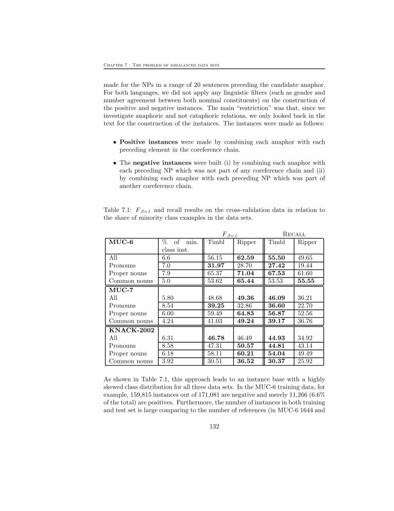
Table 7.1: F β=1 and recall results on the cross-validation data in relation tothe share of minority class examples in the data sets.

F β=1 Recall

MUC-6 % of min.class inst.

Timbl Ripper Timbl Ripper

All 6.6 56.15 62.59 55.50 49.65Pronouns 7.0 31.97 28.70 27.42 19.44Proper nouns 7.9 65.37 71.04 67.53 61.60Common nouns 5.0 53.62 65.44 53.53 55.55MUC-7All 5.80 48.68 49.36 46.09 36.21Pronouns 8.54 39.25 32.86 36.60 22.70Proper nouns 6.00 59.49 64.83 56.87 52.56Common nouns 4.24 41.03 49.24 39.17 36.76KNACK-2002All 6.31 46.78 46.49 44.93 34.92Pronouns 8.58 47.31 50.57 44.81 43.14Proper nouns 6.18 58.11 60.21 54.04 49.49Common nouns 3.92 30.51 36.52 30.37 25.92

As shown in Table 7.1, this approach leads to an instance base with a highlyskewed class distribution for all three data sets. In the MUC-6 training data, forexample, 159,815 instances out of 171,081 are negative and merely 11,266 (6.6%of the total) are positives. Furthermore, the number of instances in both trainingand test set is large comparing to the number of references (in MUC-6 1644 and

132

7.4 Balancing the data set

1627 respectively) present in both sets. In the KNACK-2002 cross-validationdata, for example, merely 6.3% of the instances is classified as positive. Butis learning performance hindered when learning from these data sets where theminority class is underrepresented?

Table 7.1 shows that although ripper performs better on the data set as awhole, it exhibits a poorer performance on the minority class than timbl does.The F β=1 results in Table 7.1 show that ripper outperforms timbl in 9 outof 12 results. But with respect to the recall scores, which is the number of cor-rectly classified minority class examples, the opposite tendency can be observed:timbl generally (11 out of 12 results) obtains a higher recall than ripper, whichimplies that timbl produces fewer false negatives. We believe that this can beexplained by the nature of both learning approaches. In a lazy learning ap-proach, all examples are stored in memory and no attempt is made to simplifythe model by eliminating low frequency events. In an eager learning approachsuch as ripper, however, possibly interesting information from the training datais either thrown away by pruning or made inaccessible by the eager construc-tion of the model. This type of approach abstracts from low-frequency events.Applied to our data sets, this implies that ripper will prune away possiblyinteresting low-frequency positive data. We will return to this issue in Section7.4.

In the previous section, we discussed several techniques proposed in the machinelearning literature for handling data sets with skewed class distributions, includ-ing up-sampling, down-sampling, adjusting misclassification costs, etc. In thefollowing section, we will investigate some of these techniques and will evaluatethe effect of class distribution and training set size on the performance of timbl

and ripper.


In order to investigate the effect of class distribution on classifier performance,it is necessary to compare the performance of the classifier on training sets witha variety of class distributions. One possible approach to create this variety ofclass distributions is to decrease the number of instances in the majority class.We investigated the effect of random down-sampling and down-sampling of thetrue negatives for both timbl and ripper. For ripper, we also changed theratio false negatives and false positives in order to improve recall. We did notperform any up-sampling experiments, since creating multiple copies from oneinstance can only guide the choice of classification in memory-based learning ifthere is a conflict among nearest neighbours. Furthermore, as already discussed

133


earlier, up-sampling can lead to rules overfitting the training data. For example,when a certain instance is copied ten times, the rule learner might quite possiblyform a rule to cover that one instance.

7.4.1 Random

In order to reduce the number of negative training instances, we experimentedwith two randomized down-sampling techniques. In a first experiment, we grad-ually down-sampled the majority class at random. We started off with no down-sampling at all and then gradually downsized the number of negative instancesin slices of 10% until there was an equal number of positive and negative traininginstances.

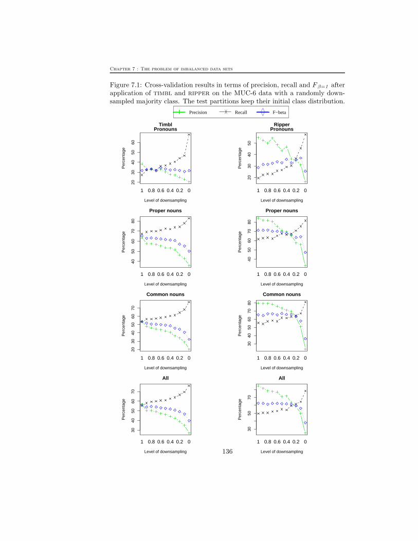
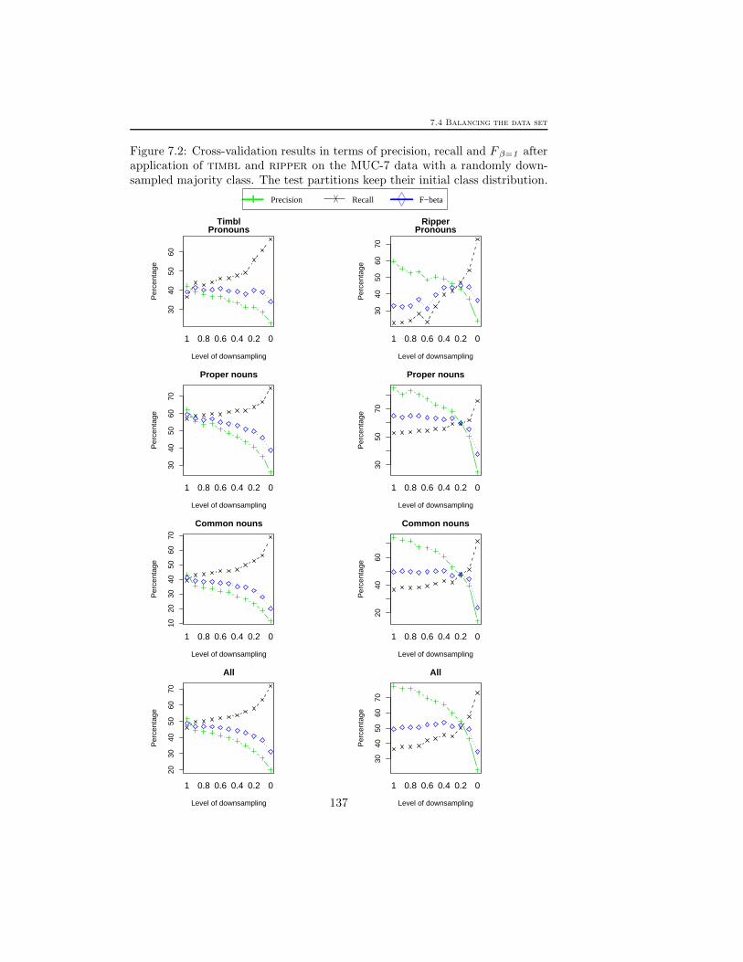
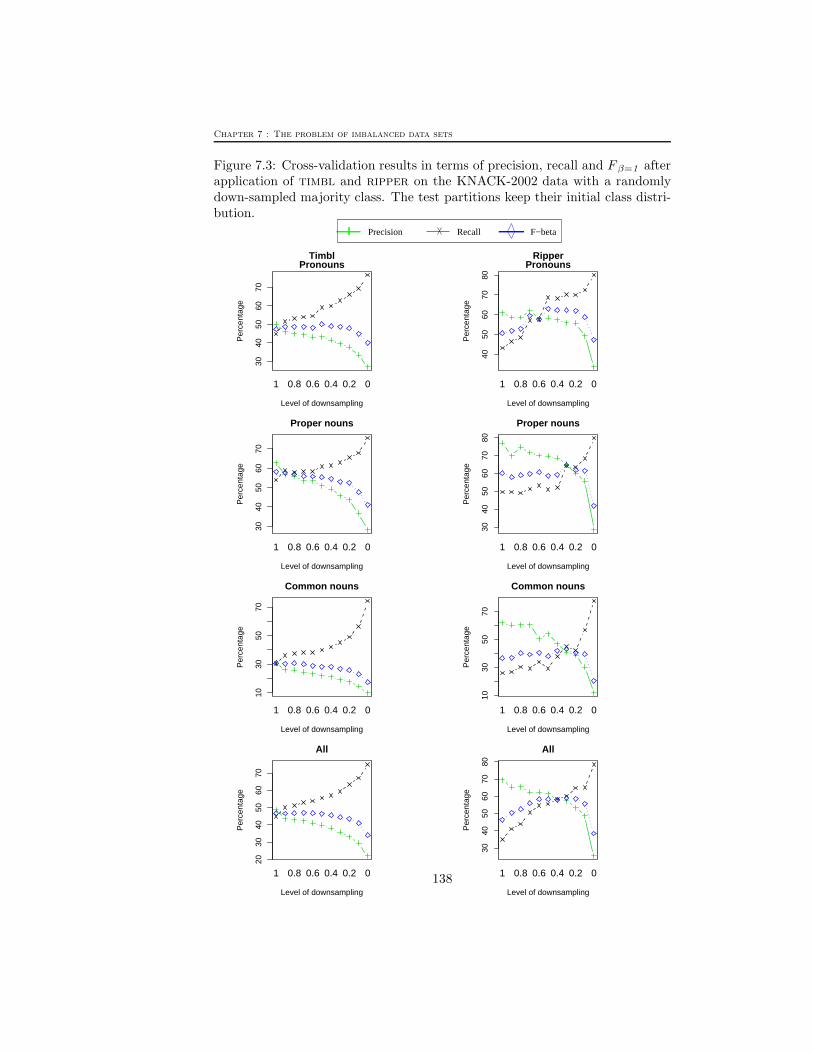
With respect to the accuracy results, we can conclude for both classifiers thatthe overall classification accuracy decreases with a decreasing rate of negativeinstances. The precision, recall and F β=1 results from the down-sampling ex-periments for both timbl and ripper are plotted in Figure 7.1, Figure 7.2 andFigure 7.3. At the X-axis, the different down-sampling levels are listed, rangingfrom 1 (no down-sampling at all) to 0 (an equal number of positive and negativeinstances). The plots for both learning methods show that a decreasing rate ofnegative instances is beneficial for the recall or the classification accuracy on theminority class instances. The plots also reveal that down-sampling is harmfulfor precision. By reducing the number of negative instances, it becomes morelikely for a test instance to be classified as positive. This implies that morenegative instances will be classified as being positive (the false positives). Butthe plots also reveal more subtle tendencies.

For timbl, the F β=1 values for the “Pronouns” data set in the whole down-sampling process remain rather constant (i.e. there are no significant differencescompared to the default scores) or they even significantly increase. On MUC-6,for example, timbl obtains a default F β=1 score of 31.97% and decreasing thenumber of negative instances with 40% leads to a top F β=1 score of 34.42%.For MUC-7, timbl obtains F β=1 scores ranging between 38.21% and 41.41%.Only the last down-sampling step in which the training set contains an equalnumber of positive and negative instances leads to a larger drop in F β=1 scores(34.21%). For KNACK-2002, the default F β=1 score of 47.31% is raised to50.02% at a down-sampling level of 0.5. For the other three data sets (“All”,“Proper nouns” and “Common nouns”), however, down-sampling does not leadto a significant increase of F β=1 values.

With respect to the ripper F β=1 values, we can conclude the following. ForMUC-6, the F β=1 values for the “Pronouns” data set are all significantly better

134


than the default result during the whole down-sampling process. ripper obtainsa default F β=1 score of 28.70% and decreasing the number of negative instanceswith 90% leads to a top F β=1 score of 37.04%. A similar tendency can beobserved for MUC-7: a default F β=1 score of 32.86% and a top F β=1 score of45.00% when down-sampling with 80%. For KNACK-2002, the default F β=1

score of 50.57% is raised to 63.00% at a down-sampling level of 0.5. For the otherthree data sets, the F β=1 values only significantly deteriorate at higher down-sampling levels. For MUC-6, for example, the F β=1 values for the “Propernouns”, “Common nouns” and “All” data sets only significantly deterioratewhen down-sampling with 30%, 70% and 50% respectively. For the KNACK-2002 data, down-sampling even leads to a significant improvement on the defaultF β=1 score: from a default 46.49% to a top score 58.84% at level 0.3 (“All”),from 36.52% to 42.84% at level 0.3 (“Common nouns”) and from 60.21% to64.60% at level 0.3 (“Proper nouns”).

For all these random down-sampling experiments we can conclude that timbl

and ripper behave differently. In Table 7.1, we showed that ripper is moresensitive to the skewedness of the classes. A comparison of results in the Figures7.1, 7.2 and 7.3 shows that down-sampling can be beneficial for the ripper

results. Furthermore, down-sampling only starts being harmful at a high down-sampling level. timbl has shown this tendency only on the “Pronouns” dataset. All these observed tendencies hold for both English data sets and the Dutchdata set.

7.4.2 Exploiting the confusion matrix

In the previous sampling experiments, all negative instances (both the truenegatives and false positives) qualified for down-sampling. In a new set ofexperiments, we also experimented with down-sampling of the true negatives.This implies that the falsely classified negative instances, the false positives,were kept in the training set, since they were considered harder to classify. Thetrue negatives were determined in a leave-one-out experiment on the differenttraining folds and then down-sampled. However, due to the highly skewed classdistribution, the level of true negatives is very high, e.g. Timbl falsely classifiesmerely 3% of the negative instances in the KNACK-2002 “All” data set. Thisimplies that these down-sampling experiments reveal the same tendencies as therandom down-sampling experiments.

As already touched upon in Section 4.3, ripper incorporates a loss ratio (Lewisand Gale 1994) (see also Section 4.3) parameter which allows the user to specifythe relative cost of two types of errors: false positives and false negatives. Itthus controls the relative weight of precision versus recall. In its default version,

135


Figure 7.1: Cross-validation results in terms of precision, recall and F β=1 afterapplication of timbl and ripper on the MUC-6 data with a randomly down-sampled majority class. The test partitions keep their initial class distribution.

Recall F−betaPrecision

2030

4050

60

TimblPronouns

Level of downsampling

Per

cent

age

1 0.8 0.6 0.4 0.2 0

2030

4050

RipperPronouns


Per

cent

age

1 0.8 0.6 0.4 0.2 0

4050

6070

80

Proper nouns


Per

cent

age

1 0.8 0.6 0.4 0.2 0

4050

6070

80

Proper nouns


Per

cent

age

1 0.8 0.6 0.4 0.2 0

2030

4050

6070

Common nouns


Per

cent

age

1 0.8 0.6 0.4 0.2 0

3040

5060

7080

Common nouns


Per

cent

age

1 0.8 0.6 0.4 0.2 0

3040

5060

70

All


Per

cent

age

1 0.8 0.6 0.4 0.2 0

3050

70

All


Per

cent

age

1 0.8 0.6 0.4 0.2 0

136


Figure 7.2: Cross-validation results in terms of precision, recall and F β=1 afterapplication of timbl and ripper on the MUC-7 data with a randomly down-sampled majority class. The test partitions keep their initial class distribution.


3040

5060

TimblPronouns


Per

cent

age

1 0.8 0.6 0.4 0.2 0

3040

5060

70

RipperPronouns

Level of downsamplingP

erce

ntag

e

1 0.8 0.6 0.4 0.2 0

3040

5060

70

Proper nouns


Per

cent

age

1 0.8 0.6 0.4 0.2 0

3050

70Proper nouns


Per

cent

age

1 0.8 0.6 0.4 0.2 0

1020

3040

5060

70

Common nouns


Per

cent

age

1 0.8 0.6 0.4 0.2 0

2040

60

Common nouns


Per

cent

age

1 0.8 0.6 0.4 0.2 0

2030

4050

6070

All


Per

cent

age

1 0.8 0.6 0.4 0.2 0

3040

5060

70

All


Per

cent

age

1 0.8 0.6 0.4 0.2 0

137


Figure 7.3: Cross-validation results in terms of precision, recall and F β=1 afterapplication of timbl and ripper on the KNACK-2002 data with a randomlydown-sampled majority class. The test partitions keep their initial class distri-bution.


3040

5060

70Timbl

Pronouns


Per

cent

age

1 0.8 0.6 0.4 0.2 0

4050

6070

80

RipperPronouns


Per

cent

age

1 0.8 0.6 0.4 0.2 0

3040

5060

70

Proper nouns


Per

cent

age

1 0.8 0.6 0.4 0.2 0

3040

5060

7080

Proper nouns


Per

cent

age

1 0.8 0.6 0.4 0.2 0

1030

5070

Common nouns


Per

cent

age

1 0.8 0.6 0.4 0.2 0

1030

5070

Common nouns


Per

cent

age

1 0.8 0.6 0.4 0.2 0

2030

4050

6070

All


Per

cent

age

1 0.8 0.6 0.4 0.2 0

3040

5060

7080

All


Per

cent

age

1 0.8 0.6 0.4 0.2 0138


ripper uses a loss ratio of 1, which indicates that the two errors have equal costs.A loss ratio greater than 1 indicates that false positive errors (where a negativeinstance is classified positive) are more costly than false negative errors (wherea positive instance is classified negative). Setting the loss ratio above 1 can beused in combination with the up-sampling of the positive minority class in orderto counterbalance the overrepresentation of the positive instances. But this isnot what we need. In all previous experiments with ripper we could observehigh precision scores and rather low recall scores. Therefore, we decided tofocus the loss ratio on the recall. For our experiments, we varied the loss ratioin ripper from 1 (default) to 0.05 (see for example also Chawla et al. (2002)for similar experiments). The motivation for this reduction of the loss ratio isdouble: (i) improve on recall and (ii) build a less restrictive set of rules for theminority class.

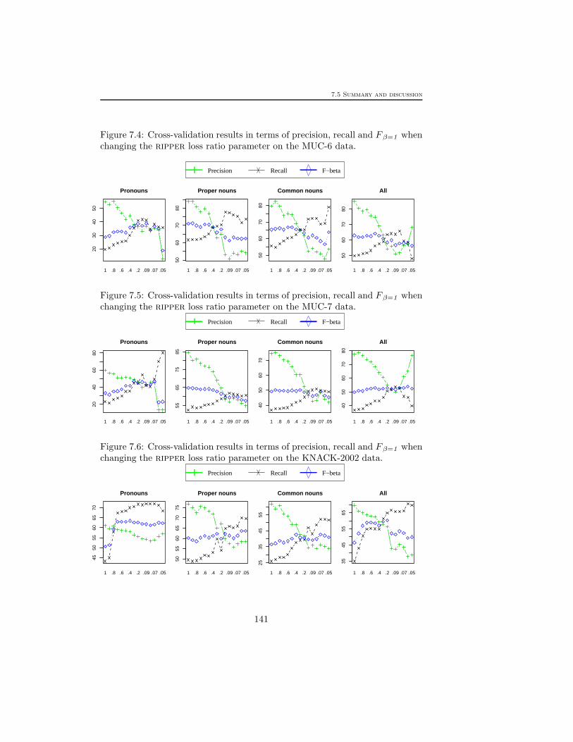
We can conclude from these experiments that, as also observed in the down-sampling experiments, a change of loss ratio is generally at the cost of overallclassification accuracy. The cross-validation precision, recall and F β=1 resultsof these experiments are displayed in Figure 7.4, Figure 7.5 and Figure 7.6.Similar tendencies as for the down-sampling experiments can be observed: thefocus on recall is harmful for precision. With respect to the F β=1 values, wecan conclude that the F β=1 values for the “Pronouns” can significantly increasewhen decreasing the loss ratio value. On MUC-6, for example, ripper obtainsa default F β=1 score of 28.70% and decreasing the loss ratio value to 0.09 leadsto a top F β=1 score of 38.80%. On MUC-7, the F β=1 score is raised up to13% when changing the loss ratio parameter. With respect to the MUC-6 andMUC-7 F β=1 values for the “Proper nouns”, “Common nouns” and “All” datasets we can observe a small increase of performance. As shown in Figure 7.6and Table 7.2, a change of the loss ratio parameter leads to a large performanceincrease for the different KNACK-2002 data sets. Furthermore, for three out ofthe four data sets, the default class distribution returns the lowest F β=1 score.

Table 7.2: Default F β=1 results for the KNACK-2002 data, in comparison withthe highest and lowest scores after change of the loss ratio parameter.

default high lowAll 46.49 60.33 (loss ratio: 0.2) 46.49Pronouns 50.57 63.49 (loss ratio: 0.4) 50.57Proper nouns 60.21 63.69 (loss ratio: 0.06) 58.61Common nouns 36.52 42.68 (loss ratio: 0.07) 36.52

The general conclusion from these experiments with loss ratio reduction is thatdecreasing the loss ratio leads to better recall at the cost of precision. For both

139


the English and Dutch data sets overall F β=1 increases can be observed. Fur-thermore, loss ratio reduction also leads to a less restrictive set of rules for theminority class, reflected in an increasing recall. With respect to the specific lossratio values, we conclude that no particular value leads to the best performanceover all data sets. This confirms our findings in the parameter optimization ex-periments (Chapter 5), which also revealed that the optimal parameter settingsof an algorithm for a given task have to be determined experimentally for eachnew data set.

7.5 Summary and discussion

In this chapter we focused on the problem of imbalanced data sets. In Sec-tion 7.2, we discussed several proposals made in the machine learning literaturefor dealing with skewed data sets and we continued with a discussion on classimbalances when learning coreference resolution. In the remainder of the chap-ter, we presented results for the MUC-6, MUC-7 and KNACK-2002 data sets.We first compared the share of minority class examples in the data sets withthe percentage of the total test errors that can be attributed to misclassifiedminority class test examples. There, we could observe a large number of falsenegatives or a large error rate for the examples from the minority class. Theseresults confirm earlier results on both machine learning and NLP data sets, e.g.by Weiss (2003) or Cardie and Howe (1997). Furthermore, we showed that al-though ripper performs better on the data set as a whole, it exhibits a poorerperformance on the recall for the minority class than timbl does.

In order to investigate the effect of class distribution on the performance oftimbl and ripper, we created a variety of class distributions through the useof down-sampling and by changing the loss ratio parameter in ripper. For thedown-sampling experiments we could conclude for the two learning methodsthat a decreasing rate of negative instances is beneficial for recall. The sameconclusion could be drawn in the experiments in wich the loss ratio parameterwas varied for ripper. These conclusions confirm earlier findings of Chan andStolfo (1998), Weiss (2003) and others. Another general conclusion is that bothdown-sampling and a change of the loss ratio parameter below 1 is harmful forprecision. This implies that more false positives will be produced.

However, both learning approaches behave quite differently in case of skewednessof the classes and they also react differently to a change in class distribution.timbl, which performs better on the minority class than ripper in case of alargely imbalanced class distribution, mainly suffers from a rebalancing of thedata set. In contrast, the ripper results are sensitive to a change of class

140


Figure 7.4: Cross-validation results in terms of precision, recall and F β=1 whenchanging the ripper loss ratio parameter on the MUC-6 data.


2030

4050

Pronouns

1 .8 .6 .4 .2 .09 .07 .05

5060

7080

Proper nouns

1 .8 .6 .4 .2 .09 .07 .05

5060

7080

Common nouns

1 .8 .6 .4 .2 .09 .07 .05

5060

7080

All

1 .8 .6 .4 .2 .09 .07 .05

Figure 7.5: Cross-validation results in terms of precision, recall and F β=1 whenchanging the ripper loss ratio parameter on the MUC-7 data.


2040

6080

Pronouns

1 .8 .6 .4 .2 .09 .07 .05

5565

7585

Proper nouns

1 .8 .6 .4 .2 .09 .07 .05

4050

6070

Common nouns

1 .8 .6 .4 .2 .09 .07 .05

4050

6070

80All

1 .8 .6 .4 .2 .09 .07 .05

Figure 7.6: Cross-validation results in terms of precision, recall and F β=1 whenchanging the ripper loss ratio parameter on the KNACK-2002 data.


4550

5560

6570

Pronouns

1 .8 .6 .4 .2 .09 .07 .05

5055

6065

7075

Proper nouns

1 .8 .6 .4 .2 .09 .07 .05

2535

4555

Common nouns

1 .8 .6 .4 .2 .09 .07 .05

3545

5565

All

1 .8 .6 .4 .2 .09 .07 .05

141


distribution or loss ratio. We believe that this different behaviour of timbl

and ripper can be explained by the nature of both learning approaches (seealso Daelemans et al. (1999) for a discussion on this topic). In a lazy learningapproach, all examples are stored in memory and no attempt is made to simplifythe model by eliminating low frequency events. In an eager learning approachsuch as ripper, however, possibly interesting information from the training datais either thrown away by pruning or made inaccessible by the eager constructionof the model. This type of approach makes abstraction from low-frequencyevents. Applied to our data sets, this implies that ripper prunes away possiblyinteresting low-frequency positive data. A decrease of the number of negativeinstances counters this pruning.

This chapter also concludes our discussion on different factors which can influ-ence a (comparative) machine learning experiment. Throughout the previouschapters we experimentally showed that apart from algorithm bias, many otherfactors such as data set selection, the selection of information sources and al-gorithm parameters and also their interaction potentially play a role in theoutcome of a machine learning experiment. We showed that changing any ofthe architectural variables can have great effects of the performance of a learn-ing method, making questionable many conclusions in the literature based ondefault settings of algorithms or on partial optimization only.

In the algorithm-comparing experiments using all information sources and de-fault parameter settings, we could observe some clear tendencies with respectto the precision and recall scores. We saw that the precision scores for timbl

were up to about 30% lower than the ones for ripper, which implies that timbl

falsely classifies more instances as being coreferential. Furthermore, with respectto the recall scores, the opposite tendency could be observed: timbl generallyobtained a higher recall than ripper. In the feature selection experiments, weobserved the large effect feature selection can have on classifier performance.Especially timbl showed a big sensitivity to a good feature subset. In the pa-rameter optimization experiments we observed that the performance differenceswithin one learning method are much larger than the method-comparing per-formance differences, which was also confirmed in the experiments exploring theinteraction between feature selection and parameter optimization. Furthermore,with respect to the selected features and parameter settings, we observed thatno particular parameter setting and no particular feature selection is optimal.This implies that the parameter settings which are optimal using all features arenot necessarily optimal when performing feature selection. We also showed thatthe features considered to be optimal for timbl can be different than the onesoptimal for ripper. In the experiments varying the class distribution of thetraining data, we showed that this was primarily beneficial for ripper. Onceagain, we showed that no particular class distribution nor loss ratio value was

142


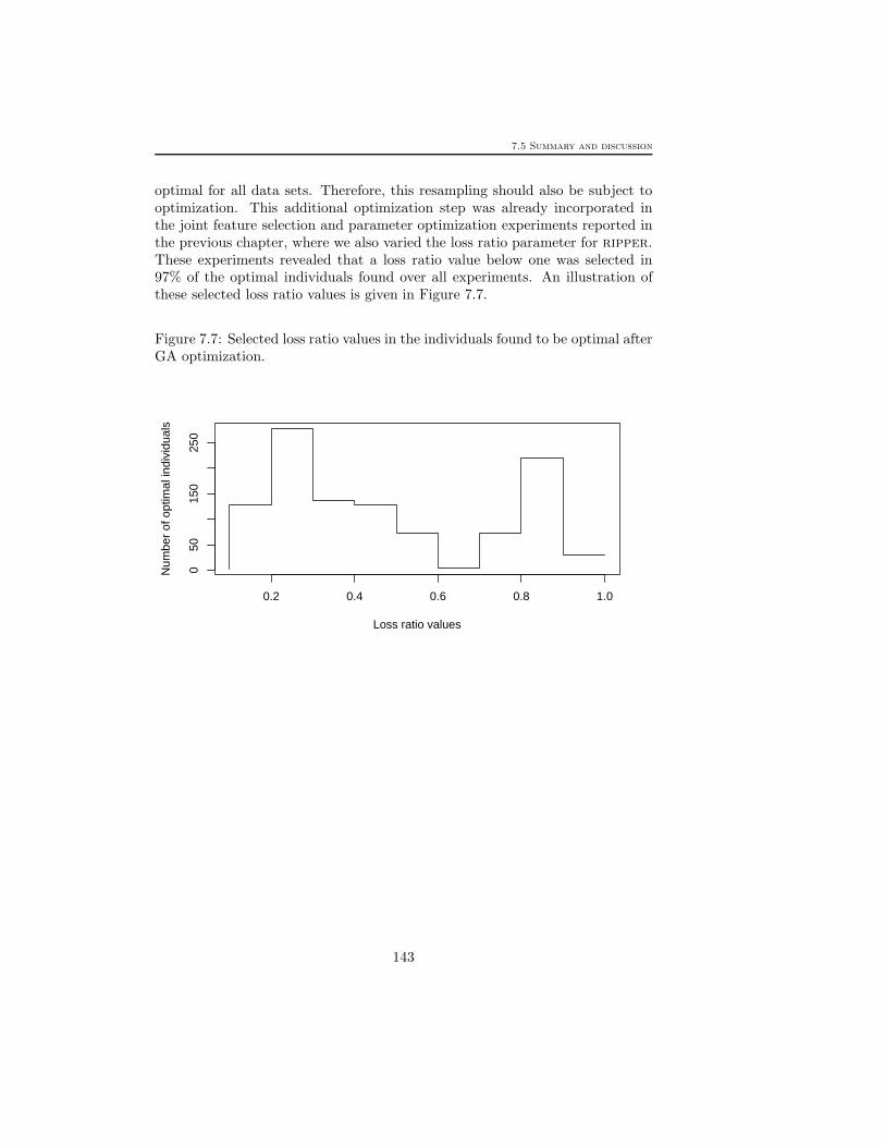
optimal for all data sets. Therefore, this resampling should also be subject tooptimization. This additional optimization step was already incorporated inthe joint feature selection and parameter optimization experiments reported inthe previous chapter, where we also varied the loss ratio parameter for ripper.These experiments revealed that a loss ratio value below one was selected in97% of the optimal individuals found over all experiments. An illustration ofthese selected loss ratio values is given in Figure 7.7.

Figure 7.7: Selected loss ratio values in the individuals found to be optimal afterGA optimization.

0.2 0.4 0.6 0.8 1.0

050

150

250

Loss ratio values

Num

ber

of o

ptim

al in

divi

dual

s

143


144

Documents

CHAPTER 7 The problem of imbalanced data sets · PDF fileCHAPTER 7 The problem of imbalanced data sets ... A central question in the discussion on data sets with an imbalanced class