Chapter 7: Money and Inflation

Instructor: Dmytro Hryshko

Money and Its Functions

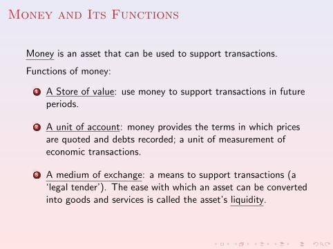
Money is an asset that can be used to support transactions.

Functions of money:

1 A Store of value: use money to support transactions in futureperiods.

2 A unit of account: money provides the terms in which pricesare quoted and debts recorded; a unit of measurement ofeconomic transactions.

3 A medium of exchange: a means to support transactions (a‘legal tender’). The ease with which an asset can be convertedinto goods and services is called the asset’s liquidity.

Types of Money

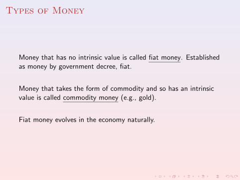
Money that has no intrinsic value is called fiat money. Establishedas money by government decree, fiat.

Money that takes the form of commodity and so has an intrinsicvalue is called commodity money (e.g., gold).

Fiat money evolves in the economy naturally.

Money supply in the economy: who controls

it and how?

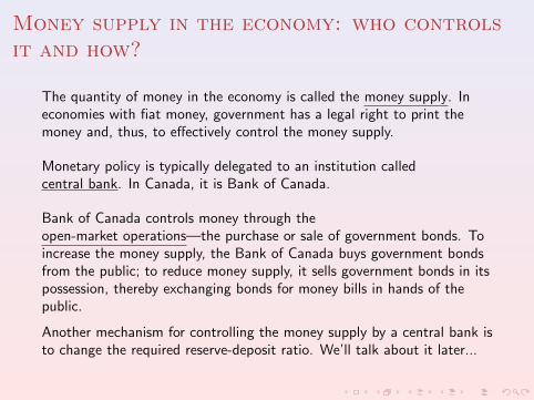
The quantity of money in the economy is called the money supply. Ineconomies with fiat money, government has a legal right to print themoney and, thus, to effectively control the money supply.

Monetary policy is typically delegated to an institution calledcentral bank. In Canada, it is Bank of Canada.

Bank of Canada controls money through theopen-market operations—the purchase or sale of government bonds. Toincrease the money supply, the Bank of Canada buys government bondsfrom the public; to reduce money supply, it sells government bonds in itspossession, thereby exchanging bonds for money bills in hands of thepublic.

Another mechanism for controlling the money supply by a central bank isto change the required reserve-deposit ratio. We’ll talk about it later...

Different measures of money supply

Money supply is the quantity of money used for transactions.

Besides coins and paper money bills, we also use checking andother accounts to support transactions.

Economists group assets into different measures of money—B, M1,M2, etc. E.g., B—the base money—is the sum of currency incirculation and required deposits of commercial banks held in thecentral bank; M1 includes currency in circulation and money inchecking accounts, etc.

The quantity theory of money

Money is used to support transactions.The quantity equation (identity):

M × V = P × T ,

where T is the total number of transactions, say, during a year; Pis the price of a typical transaction—the number of dollarsexchanged; M is the quantity of money; V is the transactions’velocity of money—a number of times one dollar bill changeshands, say, in a year.

Example

While M, P, and T can be observed, V is not, and need to bedefined from the quantity equation.

Assume the economy produces 60 loaves of bread and nothingmore (T=60); the price of one loaf is $0.50 (P=0.50); and thequantity of money in the economy is $10 (M=10).

V=(60 loaves/year ×0.50$/loaf)/$10=($30/year)/$10=3 timesper year.

The Quantity Equation of Money

The number of transactions, T , is difficult to measure. Thus, wereplace T with Y , the real output of goods and services producedin the economy.

T and Y are proportionate to each other, but not the same.We can express the quantity equation of money as:

M × V = P × Y .

V is now called the income velocity of money; P × Y is thenominal GDP.

The Money Demand Function

MP are called real money balances, and measure the quantity ofgoods you can afford given the amount of money M you have andthe typical price of a good, P.

A money demand equation can be expressed as:

(M/P)d = k × Y ,

where k is a constant of proportionality. Money demand tells youthat the desired real money balances in the economy areproportional to the total real output (income).

The Money Demand and the Quantity

Equation

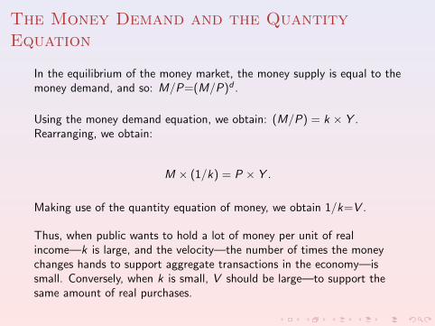
In the equilibrium of the money market, the money supply is equal to themoney demand, and so: M/P=(M/P)d .

Using the money demand equation, we obtain: (M/P) = k × Y .Rearranging, we obtain:

M × (1/k) = P × Y .

Making use of the quantity equation of money, we obtain 1/k=V .

Thus, when public wants to hold a lot of money per unit of realincome—k is large, and the velocity—the number of times the moneychanges hands to support aggregate transactions in the economy—issmall. Conversely, when k is small, V should be large—to support thesame amount of real purchases.

Constant Velocity

In general, k, and therefore V are not constant. k may depend oninnovations in financial industry (e.g., invention of ATM machinesleads to lower k).

Assume that k and V are constant.

Then, the quantity equation is:

M × V = P × Y

Money, Prices and Inflation

In percentage terms, the quantity equation becomes:

∆M

M+

∆V

V=

∆P

P+

∆Y

Y.

Since we assumed that V is a constant, ∆VV

=0, and therefore∆MM = ∆P

P + ∆YY .

In the long-run, the production of output is limited by theavailability of the factors of production. In a version of Solowmodel with technological growth, ∆Y

Y =n + g . Thus,

∆M

M=

∆P

P+ (n + g)

The Quantity Theory of Money

Note that ∆PP is the inflation rate, and n, g are exogenous

parameters.

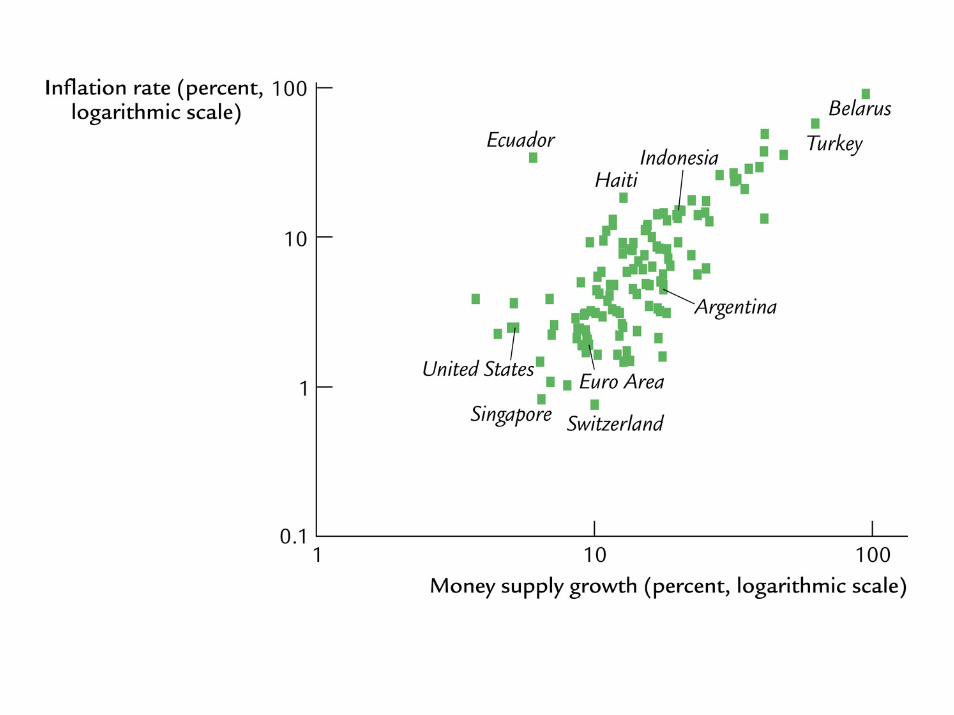
★ The quantity theory of money predicts that changes in moneysupply determine inflation in the long run.

Seigniorage

If government finances its purchases, G , by printing money,the revenue collected this way is called seigniorage.

Printing money increases money supply, and leads to inflation,and reduced purchasing power of money held by the public.

Printing money to raise revenue is conceptually similar toimposing a tax—called the inflation tax.

Inflation and Interest Rates

Let’s call the interest rate paid by banks and financial institutionsthe nominal interest rate, i ; and the increase in your purchasingpower (once money is put into the interest bearing accounts) thereal interest rate, r .

Then, r=i–π, where π is the inflation rate.

E.g., if the nominal interest rate is 10%, and the inflation rate is4%, then the real interest rate, or the increase in the purchasingpower of money put into an interest bearing bank account, is 6%.

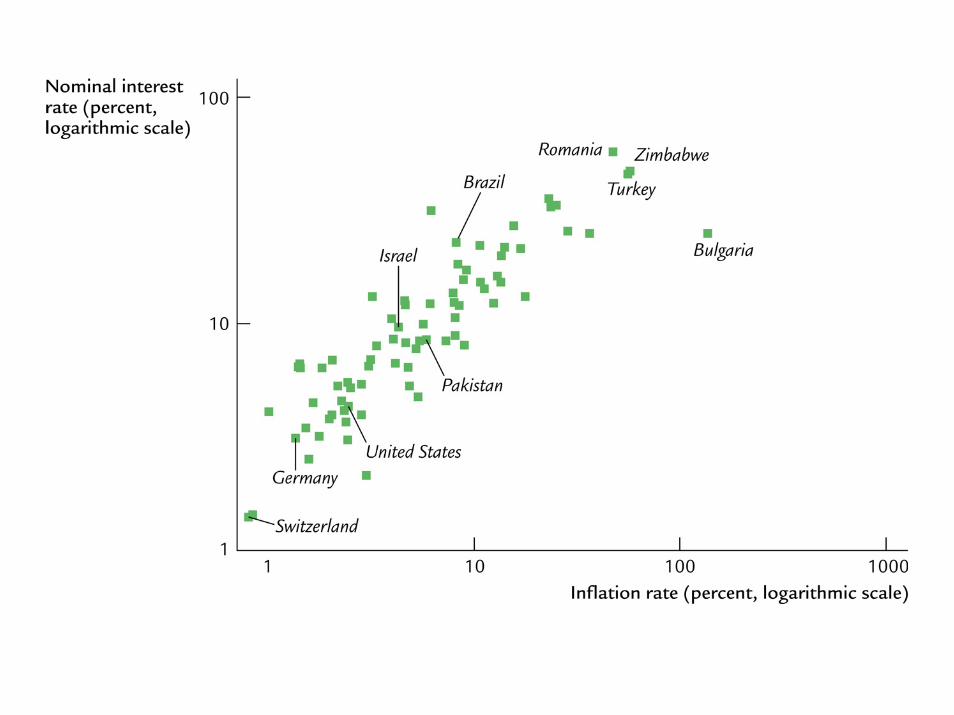
The Fisher Equation

Fisher postulated the following relation, known as theFisher equation:

i = r + π

Note that r , the real interest rate, is a function of real factors inthe economy. Thus, using the quantity theory of money, a 1%increase in money supply leads to a 1% increase in inflation and a1% increase in the nominal interest rate.

The one-to-one correspondence between inflation rate and nominalinterest rate is called the Fisher effect.

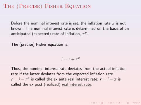
The (Precise) Fisher Equation

Before the nominal interest rate is set, the inflation rate π is notknown. The nominal interest rate is determined on the basis of ananticipated (expected) rate of inflation, πe .

The (precise) Fisher equation is:

i = r + πe

Thus, the nominal interest rate deviates from the actual inflationrate if the latter deviates from the expected inflation rate.r = i − πe is called the ex ante real interest rate; r = i − π iscalled the ex post (realized) real interest rate.

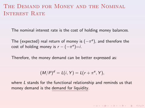
The Demand for Money and the Nominal

Interest Rate

The nominal interest rate is the cost of holding money balances.

The (expected) real return of money is (−πe), and therefore thecost of holding money is r − (−πe)=i .

Therefore, the money demand can be better expressed as:

(M/P)d = L(i ,Y ) = L(r + πe ,Y ),

where L stands for the functional relationship and reminds us thatmoney demand is the demand for liquidity.

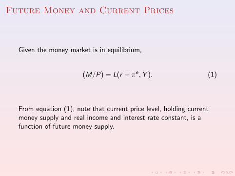
Future Money and Current Prices

Given the money market is in equilibrium,

(M/P) = L(r + πe ,Y ). (1)

From equation (1), note that current price level, holding currentmoney supply and real income and interest rate constant, is afunction of future money supply.

Costs of Inflation—the Classical Response

Our standards of living measured by W /P are determined by theproductivity of labor, and, given full flexibility in prices and wages,changes in prices should feed into changes in nominal wages, notaffecting our real purchasing power.

E.g., in Solow model the long-run (SS) level of capital per effectiveworker is determined by the production function, and exogenousparameters such as depreciation, population growth and technologicalgrowth. Real wage (per effective worker) is equal to:w = f (k∗)−MPK (k∗)× k∗, clearly a function of the economy’sproductive abilities in the long-run.

The Costs of Expected Inflation

Shoeleather costs

Menu costs

Disincentives for savings arising from the tax laws(taxing the nominal gains).

After-tax r=i(1− t)− π. If i=10%, π=10%, and t=50%, thenthe after-tax real return on savings is t × i=0.05× 0.1=0.05 lowercompared to the zero inflation rate case.

If, instead, the ex-post real returns were taxed, savings incentiveswouldn’t be distorted: After-tax r=(i − π)× (1− t).

The Costs of Unexpected Inflation

Arbitrary redistribution of wealth between debtor and creditor:debtor gains if the realized inflation rate is larger than theexpected rate; conversely, if the realized π is smaller than πe

debtor loses.

Hurts individuals with fixed pension agreements.

Hyperinflation

Hyperinflation is defined as inflation >50% per month.If the inflation rate is 50% per month, prices increase 100-fold overa year.

Additional costs of hyperinflation: relative prices do not reflectscarcity in the economy.

The causes of hyperinflation: excessive money growth due to thegovernment’s inability to finance its purchases by other means.

Usually hyperinflation ends with fiscal reforms—reduction ingovernment spending and increase in taxes.

The Classical Dichotomy

In this chapter, we assume the classical dichotomy—the irrelevanceof nominal variables (such as prices and money supply) for thedetermination of real variables (such as real output and realinterest rate).

The irrelevance of money for the determination of real variables iscalled monetary neutrality.

While being useful for the long run analysis, the assumption ofmonetary neutrality should be abandoned in the short run.

Practice: Problems 2, 5, 7, 8.