Embed Size (px)
Citation preview
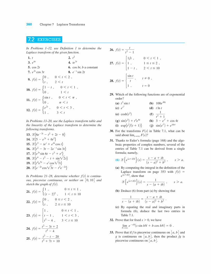
In Problems 1–12, use Definition 1 to determine theLaplace transform of the given function.
1. 2.3. 4.5. 6. cos bt, b a constant7. 8.
9.
10.
11.
12.
In Problems 13–20, use the Laplace transform table andthe linearity of the Laplace transform to determine thefollowing transforms.
13.14.15.16.17.18.19.20.
In Problems 21–28, determine whether is continu-ous, piecewise continuous, or neither on andsketch the graph of
21.
22.
23.
24.
25. f AtB !t2 " t " 20
t2 # 7t # 10
f AtB !t2 " 3t # 2
t2 " 4
f AtB ! !1 , 0 $ t 6 1 ,
t " 1 , 1 6 t 6 3 ,
t2 " 4 , 3 6 t $ 10
f AtB ! e0 , 0 $ t 6 2 ,
t , 2 $ t $ 10
f AtB ! e 1 , 0 $ t $ 1 ,At " 2B2 , 1 6 t $ 10
f AtB. 3 0, 10 4f AtB!Ee"2t cos23t " t2e"2tF!Et4e5t " et cos27tF!Et4 " t2 " t # sin22 tF!Ee3t sin 6t " t3 # etF!Et2 " 3t " 2e"t sin 3tF!Et3 " tet # e4t cos tF!E5 " e2t # 6t2F!E6e"3t " t2 # 2t " 8F
f AtB ! e e2t , 0 6 t 6 3 ,
1 , 3 6 t
f AtB ! e sin t , 0 6 t 6 p ,
0 , p 6 t
f AtB ! e1 " t , 0 6 t 6 1 ,
0 , 1 6 t
f AtB ! e0 , 0 6 t 6 2 ,
t , 2 6 t
e"t sin 2te2t cos 3tcos 2t
te3te6t
t2t
360 Chapter 7 Laplace Transforms
26.
27.
28.
29. Which of the following functions are of exponentialorder?(a) (b)(c) (d)
(e) (f)
(g) (h)(i) ( j)
30. For the transforms in Table 7.1, what can besaid about lim ?
31. Thanks to Euler’s formula (page 168) and the alge-braic properties of complex numbers, several of theentries of Table 7.1 can be derived from a singleformula; namely,
(6)
(a) By computing the integral in the definition of theLaplace transform on page 353 with !
show that
(b) Deduce (6) from part (a) by showing that
(c) By equating the real and imaginary parts informula (6), deduce the last two entries in Table 7.1.
32. Prove that for fixed s % 0, we have
33. Prove that if f is piecewise continuous on andg is continuous on , then the product fg ispiecewise continuous on .3 a, b 43 a, b 4 3 a, b 4lim
NSqe"sN As sin bN # b cos bNB ! 0 .
1s " Aa # ibB !
s " a # ibAs " aB2 # b2 .
! U e Aa#ibBt V AsB !1
s " Aa # ibB , s 7 a.
e Aa#ibBt, f AtB! U e Aa# ibBt V AsB !
s " a # ibAs " aB2 # b2 , s 7 a.
sSq F AsBF AsB sin Aet2B # esin texpEt2/ At # 1B F 3 " et2 # cos 4tsin At2B # t4e6t
1t2 # 1
cosh At2B t ln tet3
100e49 tt3 sin t
f AtB ! ! sin t
t , t & 0 ,
1 , t ! 0
f AtB ! !1/t , 0 6 t 6 1 ,
1 , 1 $ t $ 2 ,
1 " t , 2 6 t $ 10
f AtB !t
t2 " 1
7.2 EXERCISES
In Problems 1–20, determine the Laplace transform of thegiven function using Table 7.1 and the properties of thetransform given in Table 7.2. [Hint: In Problems 12–20,use an appropriate trigonometric identity.]
1. 2.3. 4.5. 6.7. 8.9. 10.
11. cosh bt 12. sin 3t cos 3t13. 14.15. 16.17. 18.
19. 20.
21. Given that use thetranslation property to compute
22. Starting with the transform use for-mula (6) for the derivatives of the Laplace transformto show that , ,and, by using induction, that
.n ! 1, 2, . . . !EtnF AsB ! n!/sn"1,
!Et2F AsB ! 2!/s3!EtF AsB ! 1/s2
!E1F AsB ! 1 /s,!Eeat cos btF.!Ecos btF AsB ! s/ As2 " b2B,m # n
t sin 2t sin 5tcos nt sin mt ,m # ncos nt cos mt ,sin 2t sin 5tt sin2 tcos3 te7t sin2 tsin2 t
te2t cos 5te$tt sin 2t
A1 " e$tB2At $ 1B4 e$2t sin 2t " e3tt22t2e$t $ t " cos 4t3t4 $ 2t2 " 1e$t cos 3t " e6t $ 13t2 $ e2tt2 " et sin 2t
Section 7.3 Properties of the Laplace Transform 365
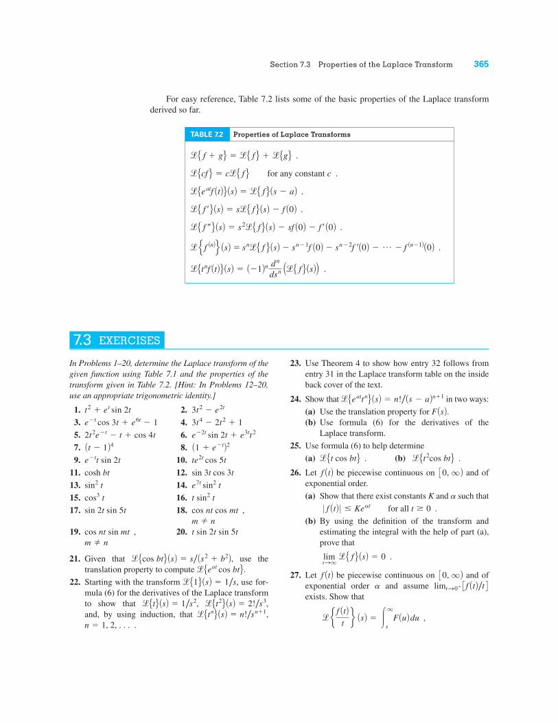
TABLE 7.2 Properties of Laplace Transforms
for any constant c .
!Etnf AtB F AsB ! A$1Bn dn
dsn A!E f F AsBB .! U f AnBV AsB ! sn!E f F AsB $ sn$1f A0B $ sn$2f ¿A0B $ p $ f An$1B A0B .!E f –F AsB ! s2!E f F AsB $ sf A0B $ f ¿ A0B .!E f ¿F AsB ! s!E f F AsB $ f A0B .!Eeatf AtB F AsB ! !E f F As $ aB .!Ecf F ! c!E f F!E f " gF ! !E f F " !EgF .For easy reference, Table 7.2 lists some of the basic properties of the Laplace transform
derived so far.
23. Use Theorem 4 to show how entry 32 follows fromentry 31 in the Laplace transform table on the insideback cover of the text.
24. Show that in two ways:(a) Use the translation property for (b) Use formula (6) for the derivatives of the
Laplace transform.25. Use formula (6) to help determine
(a) (b)
26. Let be piecewise continuous on and ofexponential order.(a) Show that there exist constants K and such that
for all (b) By using the definition of the transform and
estimating the integral with the help of part (a),prove that
27. Let be piecewise continuous on and ofexponential order and assume limexists. Show that
! e f AtBtf AsB ! !
q
sF AuB du ,
tS0" 3 f AtB / t 4a
3 0, q Bf AtBlimsSq
!E f F AsB ! 0 .
t % 0 .0 f AtB 0 & Keat
a
3 0, q Bf AtB !Et2cos btF .!Et cos btF .F AsB.!EeattnF AsB ! n! / As $ aBn"1
7.3 EXERCISES
where [Hint: First show thatand then use the result of
Problem 26.]28. Verify the identity in Problem 27 for the following
functions. (Use the table of Laplace transforms onthe inside back cover.)(a) (b)
29. The transfer function of a linear system is definedas the ratio of the Laplace transform of the outputfunction to the Laplace transform of the inputfunction when all initial conditions are zero. If alinear system is governed by the differential equation
use the linearity property of the Laplace transformand Theorem 5 on the Laplace transform of higher-order derivatives to determine the transfer function
for this system.30. Find the transfer function, as defined in Problem 29,
for the linear system governed by
31. Translation in t. Show that for c ' 0, the trans-lated function
has Laplace transform!EgF AsB ! e$cs!E f F AsB .g AtB ! e 0 , 0 6 t 6 c ,
f At $ cB , c 6 t
y– AtB " 5y¿ AtB " 6y AtB ! g AtB , t 7 0 .
H AsB ! Y AsB /G AsBy– AtB " 6y¿ AtB " 10y AtB ! g AtB , t 7 0 ,
g AtB,y AtBf AtB ! t3/ 2f AtB ! t5
dds !E f AtB / tF AsB ! $F AsBF AsB ! !E f F AsB.
366 Chapter 7 Laplace Transforms
In Problems 32–35, let be the given function translated to the right by c units. Sketch and andfind (See Problem 31.)32.33.34.35.
36. Use equation (5) to provide another derivation of theformula ! [Hint: Start with
and use induction.]
37. Initial Value Theorem. Apply the relation
(7)
to argue that for any function whose derivativeis piecewise continuous and of exponential order on
38. Verify the initial value theorem (Problem 37) for thefollowing functions. (Use the table of Laplace trans-forms on the inside back cover.)(a) 1 (b) (c) (d) cos t(e) sin t (f) (g) t cos tt2
e$te t
f A0B ! limsSq
s!E f F AsB .3 0, q B,f AtB
!E f ¿F AsB ! !q
0e$stf ¿AtB dt ! s!E f F AsB $ f A0B
!E1F AsB ! 1/sn! /sn"1.!EtnF AsB
c ! p/2f AtB ! sin t ,c ! pf AtB ! sin t ,c ! 1f AtB ! t ,c ! 2f AtB " 1 ,
!Eg AtB F AsB. g AtBf AtB f AtBg AtB
In Section 7.2 we defined the Laplace transform as an integral operator that maps a functioninto a function In this section we consider the problem of finding the function
when we are given the transform That is, we seek an inverse mapping for the Laplacetransform.
To see the usefulness of such an inverse, let’s consider the simple initial value problem
(1)
If we take the transform of both sides of equation (1) and use the linearity property of thetransform, we find
!Ey–F AsB $ Y AsB ! $ 1s2 ,
y– $ y ! $t ; y A0B ! 0 , y¿ A0B ! 1 .
F AsB. f AtBF AsB.f AtB7.4 INVERSE LAPLACE TRANSFORM
and, hence, With in (11), we obtain
and since the last equation becomes Thus Finally, settingin (11) and using and gives
Hence, and so that
With this partial fraction expansion in hand, we can immediately determine the inverseLaplace transform:
In Section 7.7, we discuss a different method (involving convolutions) for computinginverse transforms that does not require partial fraction decompositions. Moreover, the convo-lution method is convenient in the case of a rational function with a repeated quadratic factor inthe denominator. Other helpful tools are described in Problems 33–36 and 38–43.
! 3et cos 2t " 4et sin 2t # e#t .
! " 4!#1 e 2As # 1B2 " 22 f AtB # !#1 e 1s " 1
f AtB ! 3!#1 e s # 1As # 1B2 " 22 f AtB
!#1 e 2s2 " 10sAs2 # 2s " 5B As " 1B f AtB ! !#1 e 3 As # 1B " 2 A4BAs # 1B2 " 22 #1
s " 1f AtB
2s2 " 10sAs2 # 2s " 5B As " 1B !3 As # 1B " 2 A4BAs # 1B2 " 22 #
1
s " 1 .
C ! #1A ! 3, B ! 4,
A ! 3 .
0 ! #A " 8 # 5 ,
0 ! 3A A#1B " 2B 4 A1B " C A5B ,B ! 4C ! #1s ! 0B ! 4.12 ! 4B # 4.C ! #1,
2 " 10 ! 3A A0B " 2B 4 A2B " C A4B ,s ! 1C ! #1.
374 Chapter 7 Laplace Transforms
7.4 EXERCISES
In Problems 1–10, determine the inverse Laplace trans-form of the given function.
1. 2.
3. 4.
5. 6.
7. 8.
9. 10. s # 12s2 " s " 6
3s # 152s2 # 4s " 10
1s5
2s " 16s2 " 4s " 13
3A2s " 5B31s2 " 4s " 8
4s2 " 9
s " 1s2 " 2s " 10
2s2 " 4
6As # 1B4In Problems 11–20, determine the partial fraction expan-sions for the given rational function.
11. 12.
13.
14.
15. 16.
17. 18. 3s2 " 5s " 3s4 " s3
3s " 5s As2 " s # 6B
#5s # 36As " 2B As2 " 9B8s # 2s2 # 14As " 1B As2 # 2s " 5B#8s2 # 5s " 9As " 1B As2 # 3s " 2B
#2s2 # 3s # 2s As " 1B2
#s # 7As " 1B As # 2Bs2 # 26s # 47As # 1B As " 2B As " 5B
19. 20.
In Problems 21–30, determine
21.
22.
23.
24.
25.
26.
27.
28.
29.
30.
31. Determine the Laplace transform of each of thefollowing functions:
(a)
(b)
(c)Which of the preceding functions is the inverseLaplace transform of ?
32. Determine the Laplace transform of each of thefollowing functions:
(a)
(b) f2 AtB ! ! et , t $ 5, 8 ,
6 , t ! 5 ,
0 , t ! 8 .
f1 AtB ! e t , t ! 1, 2, 3, . . . ,
et , t $ 1, 2, 3, . . . .
1 /s2
f3 AtB ! t .
f2 AtB ! !5 , t ! 1 ,
2 , t ! 6 ,
t , t $ 1, 6 .
f1 AtB ! e0 , t ! 2 ,
t , t $ 2 .
sF AsB # F AsB !2s " 5
s2 " 2s " 1
sF AsB " 2F AsB !10s2 " 12s " 14
s2 # 2s " 2
s2F AsB " sF AsB # 6F AsB !s2 " 4s2 " s
s2F AsB # 4F AsB !5
s " 1
F AsB !7s3 # 2s2 # 3s " 6
s3 As # 2BF AsB !
7s2 " 23s " 30As # 2B As2 " 2s " 5BF AsB !
7s2 # 41s " 84As # 1B As2 # 4s " 13BF AsB !
5s2 " 34s " 53As " 3B2 As " 1BF AsB !
s " 11As # 1B As " 3BF AsB !
6s2 # 13s " 2s As # 1B As # 6B
!#1EFF .sAs # 1B As2 # 1B1As # 3B As2 " 2s " 2B
Section 7.4 Inverse Laplace Transform 375
(c)Which of the preceding functions is the inverseLaplace transform of ?
Theorem 6 in Section 7.3 can be expressed in terms of theinverse Laplace transform as
where . Use this equation in Problems33–36 to compute
33. 34.
35. 36.
37. Prove Theorem 7 on the linearity of the inversetransform. [Hint: Show that the right-hand side ofequation (3) is a continuous function on whose Laplace transform is
38. Residue Computation. Let be a rationalfunction with deg P % deg Q and suppose is anonrepeated linear factor of Prove that the por-tion of the partial fraction expansion of corresponding to is
where A (called the residue) is given by the formula
39. Use the residue computation formula derived inProblem 38 to determine quickly the partial fractionexpansion for
40. Heaviside’s Expansion Formula.† Let andbe polynomials with the degree of less
than the degree of Let
where the ’s are distinct real numbers. Show that
!#1 e P
Qf AtB !an
i!1
P AriBQ¿AriB erit .
ri
Q AsB ! As # r1B As # r2B p As # rnB ,Q AsB. P AsBQ AsB P AsBF AsB !2s " 1
s As # 1B As " 2B .
A ! limsSr
As " rBP AsBQ AsB .
As " r ,
s # rP AsB /Q AsBQ AsB. s # r
P AsB /Q AsBF1 AsB " F2 AsB. 4 3 0, q BF AsB ! arctan A1/sBF AsB ! ln as2 " 9
s2 " 1b
F AsB ! ln as # 4s # 3
bF AsB ! ln as " 2s # 5
b!#1EFF.f ! !#1EFF
!#1 e dnFdsn f AtB ! A#tBnf AtB ,
1 / As # 1Bf3 AtB ! et .
† Historical Footnote: This formula played an important role in the “operational solution” to ordinary differentialequations developed by Oliver Heaviside in the 1890s.
41. Use Heaviside’s expansion formula derived in Prob-lem 40 to determine the inverse Laplace transform of
42. Complex Residues. Let be a rationalfunction with deg P % deg Q and suppose
is a nonrepeated quadratic factor of Q.(That is, are complex conjugate zeros of Q.)Prove that the portion of the partial fraction expansionof corresponding to is
A As # aB " bBAs # aB2 " b2 ,
As # aB2 " b2P AsB /Q AsBa & ib
As # aB2 " b2
P AsB /Q AsBF AsB !
3s2 # 16s " 5As " 1B As # 3B As # 2B .
376 Chapter 7 Laplace Transforms
where the complex residue is given bythe formula
(Thus we can determine B and A by taking the realand imaginary parts of the limit and dividing themby
43. Use the residue formulas derived in Problems 38 and42 to determine the partial fraction expansion for
F AsB !6s2 " 28As2 # 2s " 5B As " 2B .
b.BbB " ibA ! lim
sSa"ib
3 As # aB2 " b2 4P AsBQ AsB .
bB " ibA
Our goal is to show how Laplace transforms can be used to solve initial value problems forlinear differential equations. Recall that we have already studied ways of solving such initialvalue problems in Chapter 4. These previous methods required that we first find a generalsolution of the differential equation and then use the initial conditions to determine the desiredsolution. As we will see, the method of Laplace transforms leads to the solution of the initialvalue problem without first finding a general solution.
Other advantages to the transform method are worth noting. For example, the techniquecan easily handle equations involving forcing functions having jump discontinuities, as illus-trated in Section 7.1. Further, the method can be used for certain linear differential equationswith variable coefficients, a special class of integral equations, systems of differential equa-tions, and partial differential equations.
7.5 SOLVING INITIAL VALUE PROBLEMS
Method of Laplace TransformsTo solve an initial value problem:
(a) Take the Laplace transform of both sides of the equation.(b) Use the properties of the Laplace transform and the initial conditions to obtain an
equation for the Laplace transform of the solution and then solve this equation forthe transform.
(c) Determine the inverse Laplace transform of the solution by looking it up in a table orby using a suitable method (such as partial fractions) in combination with the table.
In step (a) we are tacitly assuming the solution is piecewise continuous on and ofexponential order. Once we have obtained the inverse Laplace transform in step (c), we canverify that these tacit assumptions are satisfied.
Solve the initial value problem
(1) y– # 2y¿ " 5y ! #8e#t ; y A0B ! 2 , y¿ A0B ! 12 .
30, q BExample 1
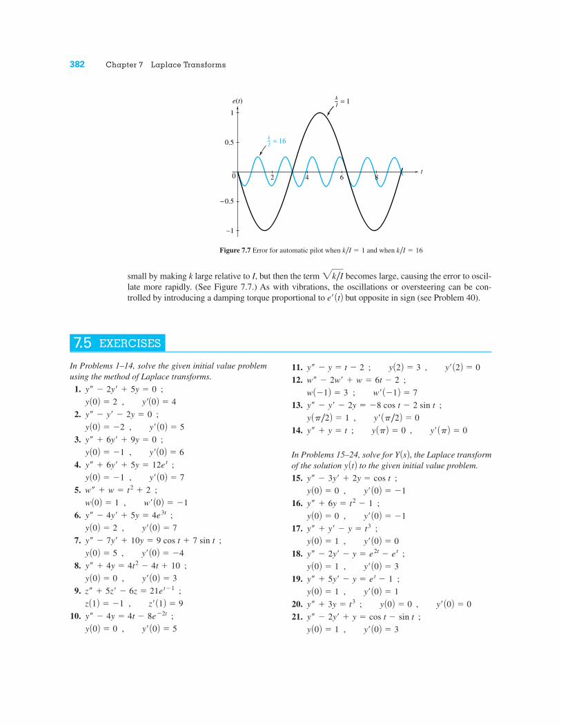
small by making k large relative to I, but then the term becomes large, causing the error to oscil-late more rapidly. (See Figure 7.7.) As with vibrations, the oscillations or oversteering can be con-trolled by introducing a damping torque proportional to but opposite in sign (see Problem 40).e¿ AtB2k/I
382 Chapter 7 Laplace Transforms
e(t)
8642
1
0.5k = 16I
I
0
−0.5
−1
t
k = 1
Figure 7.7 Error for automatic pilot when and when k/I ! 16k/I ! 1
7.5 EXERCISES
In Problems 1–14, solve the given initial value problemusing the method of Laplace transforms.
1.
2.
3.
4.
5.
6.
7.
8.
9.
10.y A0B ! 0 , y¿ A0B ! 5y– " 4y ! 4t " 8e"2t ;z A1B ! "1 , z¿ A1B ! 9z– # 5z¿ " 6z ! 21et"1 ;y A0B ! 0 , y¿ A0B ! 3y– # 4y ! 4t2 " 4t # 10 ;y A0B ! 5 , y¿ A0B ! "4y– " 7y¿ # 10y ! 9 cos t # 7 sin t ;y A0B ! 2 , y¿ A0B ! 7y– " 4y¿ # 5y ! 4e3t ;w A0B ! 1 , w¿ A0B ! "1w– # w ! t2 # 2 ;y A0B ! "1 , y¿ A0B ! 7y– # 6y¿ # 5y ! 12et ;y A0B ! "1 , y¿ A0B ! 6y– # 6y¿ # 9y ! 0 ;y A0B ! "2 , y¿ A0B ! 5y– " y¿ " 2y ! 0 ;y A0B ! 2 , y¿A0B ! 4y– " 2y¿ # 5y ! 0 ;
11.12.
13.
14.
In Problems 15–24, solve for the Laplace transformof the solution to the given initial value problem.15.
16.
17.
18.
19.
20.21.
y A0B ! 1 , y¿ A0B ! 3y– " 2y¿ # y ! cos t " sin t ;y– # 3y ! t3 ; y A0B ! 0 , y¿ A0B ! 0y A0B ! 1 , y¿ A0B ! 1y– # 5y¿ " y ! et " 1 ;y A0B ! 1 , y¿ A0B ! 3y– " 2y¿ " y ! e2t " et ;y A0B ! 1 , y¿ A0B ! 0y– # y¿ " y ! t3 ;y A0B ! 0 , y¿ A0B ! "1y– # 6y ! t2 " 1 ;y A0B ! 0 , y¿ A0B ! "1y– " 3y¿ # 2y ! cos t ;
y AtB Y AsB,y– # y ! t ; y ApB ! 0 , y¿ ApB ! 0y Ap/2B ! 1 , y¿ Ap/2B ! 0y– " y¿ " 2y ! "8 cos t " 2 sin t ;w A"1B ! 3 ; w¿ A"1B ! 7w– " 2w¿ # w ! 6t " 2 ;y– " y ! t " 2 ; y A2B ! 3 , y¿ A2B ! 0
22.
23.where
24.where
In Problems 25–28, solve the given third-order initialvalue problem for using the method of Laplacetransforms.25.
26.
27.
28.
In Problems 29–32, use the method of Laplace trans-forms to find a general solution to the given differentialequation by assuming and where aand b are arbitrary constants.29. 30.31.32.
33. Use Theorem 6 in Section 7.3 to show that
where Y AsB ! !EyF AsB .!Et2y¿ AtB F AsB ! sY–AsB # 2Y¿AsB ,y– " 5y¿ # 6y ! "6te2t
y– # 2y¿ # 2y ! 5y– # 6y¿ # 5y ! ty– " 4y¿ # 3y ! 0
y¿ A0B ! b,y A0B ! a
y A0B ! 0 , y¿ A0B ! 2 , y– A0B ! "4y‡ # y– # 3y¿ " 5y ! 16e"t ;y A0B ! "4 , y¿ A0B ! 4 , y– A0B ! "2y‡ # 3y– # 3y¿ # y ! 0 ;y A0B ! 1 , y¿ A0B ! 4 , y– A0B ! "2y‡ # 4y– # y¿ " 6y ! "12 ;y A0B ! 1 , y¿ A0B ! 1 , y– A0B ! 3y‡ " y– # y¿ " y ! 0 ;
y AtBg AtB ! e 1 , t 6 3 ,
t , t 7 3
y– " y ! g AtB ; y A0B ! 1 , y¿ A0B ! 2 ,
g AtB ! e t , t 6 2 ,
5 , t 7 2
y– # 4y ! g AtB ; y A0B ! "1 ; y¿ A0B ! 0 ,y A0B ! 2 , y¿ A0B ! "1y– " 6y¿ # 5y ! te t ;
Section 7.6 Transforms of Discontinuous and Periodic Functions 383
34. Use Theorem 6 in Section 7.3 to show that
where
In Problems 35–38, find solutions to the given initialvalue problem.35.
36.
37.
[Hint:38.
39. Determine the error for the automatic pilot inExample 5 if the shaft is initially at rest in the zerodirection and the desired direction is where a is a constant.
40. In Example 5 assume that in order to controloscillations a component of torque proportional to
but opposite in sign, is also fed back to thesteering shaft. Show that equation (17) is nowreplaced by
where is a positive constant. Determine the errorfor the automatic pilot with mild damping (i.e.,
if the steering shaft is initially at rest inthe zero direction and the desired direction is givenby where a is a constant.
41. In Problem 40 determine the error when thedesired direction is given by where a is aconstant.
g AtB ! at,e AtBg AtB ! a,
m 6 22IkBe AtB m
Iy– AtB ! "ke AtB " me¿ AtB ,e¿ AtB,
g AtB ! a,
e AtBy A0B ! 0 , y¿ A0B ! 3y– # ty¿ " y ! 0 ;
!"1E1 / As2 # 1B2F AtB ! Asin t " t cos tB /2. 4y A0B ! 1 , y¿ A0B ! 0ty– " 2y¿ # ty ! 0 ;y A0B ! 2 , y¿ A0B ! "1ty– " ty¿ # y ! 2 ;y A0B ! 0 , y¿ A0B ! 0y– # 3ty¿ " 6y ! 1 ;
Y AsB ! !EyF AsB .!Et2y– AtB F AsB ! s2Y– AsB # 4sY¿ AsB # 2Y AsB ,
7.6 TRANSFORMS OF DISCONTINUOUS AND PERIODIC FUNCTIONS
In this section we study special functions that often arise when the method of Laplace trans-forms is applied to physical problems. Of particular interest are methods for handling functionswith jump discontinuities. Jump discontinuities occur naturally in physical problems such aselectric circuits with on/off switches. To handle such behavior, Oliver Heaviside introduced thefollowing step function.
When t is a positive integer, say then the recursive relation (19) can be repeatedlyapplied to obtain
It follows from the definition (18) that so we find
Thus, the gamma function extends the notion of factorial!As an application of the gamma function, let’s return to the problem of determining the
Laplace transform of an arbitrary power of t. We will verify that the formula
(20)
holds for every constant By definition,
Let’s make the substitution Then and we find
Notice that when is a nonnegative integer, then and so formula (20) reduces to the familiar formula for !EtnF. ! An " 1B # n!,r # n
#1
sr" 1 !q
0e$ uur
du #! Ar " 1B
sr" 1 .
!EtrF AsB # !q
0e$ u au
sb r a1
sbdu
du # s dt,u # st.
!EtrF AsB # !q
0e$ sttr
dt .
r 7 $ 1 .
!EtrF AsB !" Ar # 1B
sr# 1
" An # 1B ! n! .
! A1B # 1,
# n An $ 1B An $ 2B p 2! A1B .! An " 1B # n! AnB # n An $ 1B! An $ 1B # p
t # n,
Section 7.6 Transforms of Discontinuous and Periodic Functions 393
7.6 EXERCISES
In Problems 1–4, sketch the graph of the given functionand determine its Laplace transform.
1.2.3.4.
In Problems 5–10, express the given function using windowand step functions and compute its Laplace transform.
5. g AtB # "0 , 0 6 t 6 1 ,
2 , 1 6 t 6 2 ,
1 , 2 6 t 6 3 ,
3 , 3 6 t
tu At $ 1Bt2u At $ 2Bu At $ 1B $ u At $ 4BAt $ 1B2u At $ 1B 6. g AtB # e 0 , 0 6 t 6 2 ,
t " 1 , 2 6 t
g(t)
t
2
1
01 2
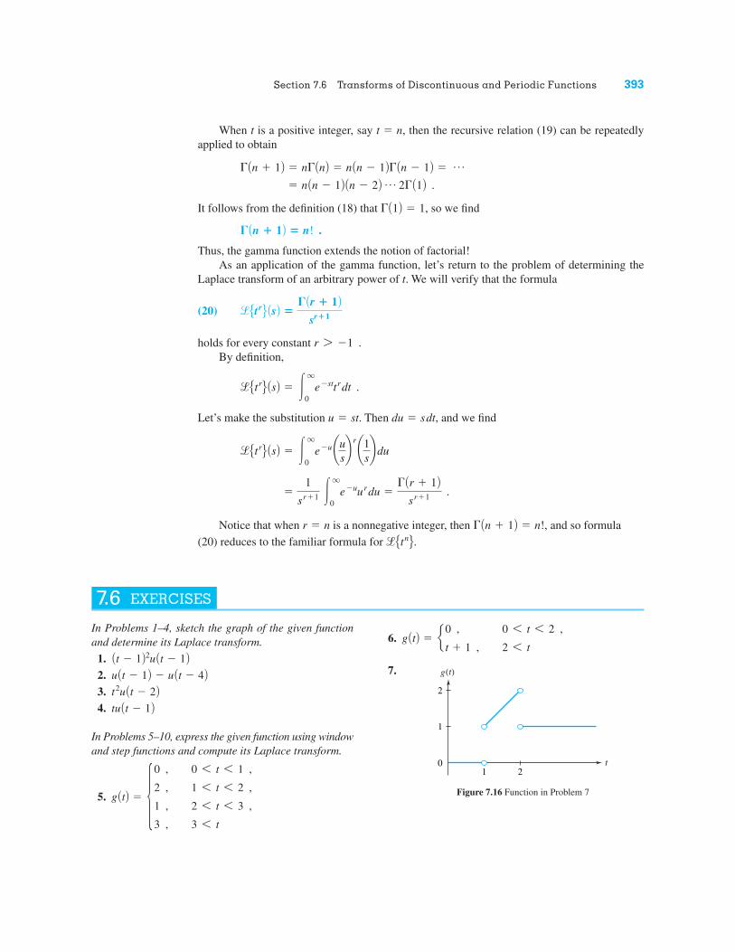
Figure 7.16 Function in Problem 7
7.
394 Chapter 7 Laplace Transforms
1
t
g(t)
−1
sin t
Figure 7.17 Function in Problem 8
g (t)
t
1
10 2 3 4
Figure 7.18 Function in Problem 9
t43
(t − 1)2
21
1
2
3
0
g(t)
Figure 7.19 Function in Problem 10
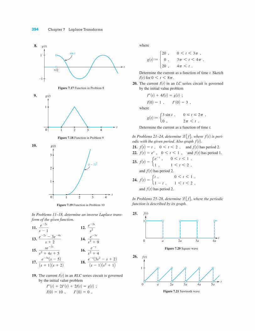
8.
9.
10.
In Problems 11–18, determine an inverse Laplace trans-form of the given function.
11. 12.
13. 14.
15. 16.
17. 18.
19. The current in an RLC series circuit is governedby the initial value problem
I A0B # 10 , I¿ A0B # 0 ,I– AtB " 2I¿ AtB " 2I AtB # g AtB ;
I AtBe$ s A3s2 $ s " 2BAs $ 1B As2 " 1Be$ 3s As $ 5BAs " 1B As " 2B
e$ s
s2 " 4se$ 3s
s2 " 4s " 5
e$ 3s
s2 " 9e$ 2s $ 3e$ 4s
s " 2
e$ 3s
s2e$ 2s
s $ 1
where
Determine the current as a function of time t. Sketchfor
20. The current in an LC series circuit is governedby the initial value problem
where
Determine the current as a function of time t.
In Problems 21–24, determine , where is peri-odic with the given period. Also graph 21. and has period 2.22. and has period 1.
23.
and has period 2.
24.
and has period 2.
In Problems 25–28, determine where the periodicfunction is described by its graph.
!E f F,f AtBf AtB # e t , 0 6 t 6 1 ,
1 $ t , 1 6 t 6 2 ,
f AtBf AtB # e e$ t , 0 6 t 6 1 ,
1 , 1 6 t 6 2 ,
f AtBf AtB # et , 0 6 t 6 1 , f AtBf AtB # t , 0 6 t 6 2 ,
f AtB. f AtB!E f Fg AtB J e 3 sin t , 0 % t % 2p ,
0 , 2p 6 t .
I¿ A0B # 3 ,I A0B # 1 ,
I– AtB " 4I AtB # g AtB ;
I AtB0 6 t 6 8p.I AtBg AtB J " 20 , 0 6 t 6 3p ,
0 , 3p 6 t 6 4p ,
20 , 4p 6 t .
2a
f (t)
ta 3a 4a0
1
Figure 7.20 Square wave
5a2a
f (t)
ta 3a 4a0
1
Figure 7.21 Sawtooth wave
25.
26.
Section 7.6 Transforms of Discontinuous and Periodic Functions 395
2a
f (t)
ta 3a 4a0
1
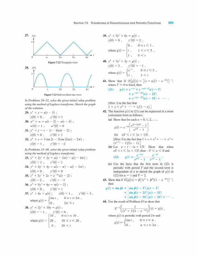
Figure 7.22 Triangular wave
f (t)
t0
1
Figure 7.23 Half-rectified sine wave
27.
28.
In Problems 29–32, solve the given initial value problemusing the method of Laplace transforms. Sketch the graphof the solution.29.
30.
31.
32.
In Problems 33–40, solve the given initial value problemusing the method of Laplace transforms.33.
34.
35.
36.
37.
where
38.
where g AtB # "10 , 0 % t % 10 ,
20 , 10 6 t 6 20 ,
0 , 20 6 t
y¿ A0B # 0 ,y A0B # $ 1 , y– " 2y¿ " 10y # g AtB ;
g AtB # e sin t , 0 % t % 2p ,
0 , 2p 6 t
y¿ A0B # 3 ,y– " 4y # g AtB ; y A0B # 1 , y A0B # 0 , y¿ A0B # 1y– " 5y¿ " 6y # tu At $ 2B ;z A0B # 2 , z¿ A0B # $ 3z– " 3z¿ " 2z # e$ 3t
u At $ 2B ;y A0B # 0 , y¿ A0B # 0y– " 4y¿ " 4y # u At $ pB $ u At $ 2pB ;y A0B # 1 , y¿ A0B # 1y– " 2y¿ " 2y # u At $ 2pB $ u At $ 4pB ;y A0B # 1 , y¿ A0B # $ 2y– " y # 3 sin 2t $ 3 Asin 2tBu At $ 2pB ;y A0B # 0 , y¿ A0B # 1y– " y # t $ At $ 4Bu At $ 2B ;w A0B # 1 , w¿ A0B # 0w– " w # u At $ 2B $ u At $ 4B ;y¿ A0B # 1y A0B # 0 , y– " y # u At $ 3B ;
39.
where
40.
where
41. Show that if where is fixed, then
(21)
[Hint: Use the fact that
42. The function in (21) can be expressed in a moreconvenient form as follows:(a) Show that for each n # 0, 1, 2, . . . ,
for[Hint: Use the fact that #
(b) Let Show that when & then and
(22)
(c) Use the facts that the first term in (22) isperiodic with period T and the second term isindependent of n to sketch the graph of in(22) for and
43. Show that if #then
44. Use the result of Problem 43 to show that
where is periodic with period and
g AtB J e sin t , 0 % t % p ,
0 , p % t % 2p .
2pg AtB!$ 1 e 1As2 " 1B A1 $ e$ psB f AtB # g AtB ,# 3 sin B At $ 3TB 4u At $ 3TB # p .# 3 sin B At $ 2TB 4u At $ 2TBg AtB ! sin Bt # 3 sin B At $ TB 4u At $ TB
b 3 As2 " b2B A1 $ e$ TsB 4 $ 1,!EgF AsB T # 2.a # 1g AtB
g AtB !e$AY
eAT $ 1$
e$At
eAT $ 1 .
$ T 6 y 6 0t 6 An " 1BT,nTy # t $ An " 1BT.
Axn" 1 $ 1B / Ax $ 1B. 4 1 " x " x2 " p " xn
nT 6 t 6 An " 1BT.
g AtB # e$ at ce An" 1BaT $ 1eaT $ 1
dg AtB1 " x " x2 " p # 1 / A1 $ xB. 4# e$AAt$ 3TBu At $ 3TB # p .
# e$AAt$ 2TBu At $ 2TBg AtB ! e$ at # e$AAt$ TBu At $ TBT 7 0!EgF AsB # 3 As " aB A1 $ e$ TsB 4 $ 1,
g AtB # e e$ t , 0 % t 6 3 ,
1 , 3 6 t
y¿ A0B # $ 1 ,y A0B # 2 , y– " 3y¿ " 2y # g AtB ;
g AtB # "0 , 0 % t 6 1 ,
t , 1 6 t 6 5 ,
1 , 5 6 t
y¿ A0B # 2 ,y A0B # 0 , y– " 5y¿ " 6y # g AtB ;
396 Chapter 7 Laplace Transforms
In Problems 45 and 46, use the method of Laplace trans-forms and the results of Problems 41 and 42 to solve theinitial value problem.
where is the periodic function defined in the statedproblem.45. Problem 22 46. Problem 25 with
In Problems 47–50, find a Taylor series for aboutAssuming the Laplace transform of can be
computed term by term, find an expansion for inpowers of . If possible, sum the series.47. 48.
49. 50.
51. Using the recursive relation (19) and the fact thatdetermine
(a) (b)52. Use the recursive relation (19) and the fact that
to show that
where n is a positive integer.
53. Verify (15) in Theorem 9 for the functiontaking the period as Repeat, taking
the period as
54. By replacing s by in the Maclaurin series expan-sion for arctan s, show that
55. Find an expansion for in powers of . Usethe expansion for to obtain an expansion for
in terms of Assuming theinverse Laplace transform can be computed term byterm, show that
[Hint: Use the result of Problem 52.]
56. Use the procedure discussed in Problem 55 to showthat
!$ 1Es$ 3/2e$ 1/sF AtB #11p
sin 21t .
!$ 1Es$ 1/2e$ 1/sF AtB #11pt
cos 21t .
1 /sn" 1/2.s$ 1/2e$ 1/se$ 1/s
1 /se$ 1/s
arctan 1s
#1s
$1
3s3 "1
5s5 $1
7s7 " p .
1 /s4p.
2p.ƒ AtB # sin t,
!$ 1 U s$ An" 1/2B V AtB #2ntn$ 1/2
1 # 3 # 5 p A2n $ 1B1p ,
! A1 /2B # 1p !Et7/2F .!Et$ 1/2F .! A1 /2B # 1p,
f AtB # e$ t2f AtB #
1 $ cos tt
f AtB # sin tf AtB # et
1 /s!E f F AsBf AtBt # 0.f AtB
a # 1
f AtBy A0B # 0 , y¿ A0B # 0 ,y– " 3y¿ " 2y # f AtB ;
57. Find an expansion for ln in powers of. Assuming the inverse Laplace transform can be
computed term by term, show that
58. The unit triangular pulse is defined by
(a) Sketch the graph of . Why is it so named?Why is its symbol appropriate?
(b) Show that .
(c) Find the Laplace transform of .
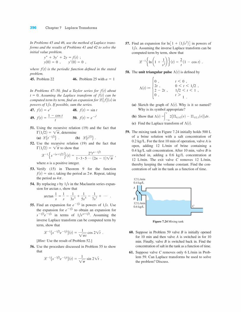
59. The mixing tank in Figure 7.24 initially holds 500 Lof a brine solution with a salt concentration of 0.2 kg/L. For the first 10 min of operation, valve A isopen, adding 12 L/min of brine containing a 0.4 kg/L salt concentration. After 10 min, valve B isswitched in, adding a 0.6 kg/L concentration at 12 L/min. The exit valve C removes 12 L/min,thereby keeping the volume constant. Find the con-centration of salt in the tank as a function of time.
¶ AtB¶ AtB #!t
$ q2Eß0,1/2 AtB $ ß1/2,1 AtB Fdt¶ AtB
¶ AtB J " 0 , t 6 0 ,2t , 0 6 t 6 1 /2 ,2 $ 2t , 1 /2 6 t 6 1 ,0 , t 7
1 .
¶ AtB!$ 1 e ln a1 "
1s2b f AtB #
2t
A1 $ cos tB .1 /s
3 1 " A1 /s2B 4
C
A
12 L/min0.4 kg/L
12 L/min0.6 kg/L
B
Figure 7.24 Mixing tank
60. Suppose in Problem 59 valve B is initially openedfor 10 min and then valve A is switched in for 10min. Finally, valve B is switched back in. Find theconcentration of salt in the tank as a function of time.
61. Suppose valve C removes only 6 L/min in Prob-lem 59. Can Laplace transforms be used to solvethe problem? Discuss.
The inverse Laplace transform of is the impulse response function
To solve the initial value problem, we need the solution to the corresponding homoge-neous problem. The auxiliary equation for the homogeneous equation is which has roots Thus a general solution is Choos-ing and so that the initial conditions in (21) are satisfied, we obtain
Hence, a formula for the solution to the initial value problem (21) is
Ah * gB AtB ! yk AtB "12 !
t
0e#At#yB sin 32 At # yB 4g AyBdy ! 2e#t cos 2t .
yk AtB " 2e#t cos 2t.C2C1
C1e#t cos 2t ! C2e
#t sin 2t.r " #1 $ 2i.r 2 ! 2r ! 5 " 0,
"12
e#t sin 2t .
h AtB " !#1EHF AtB "12
!#1 e 2As ! 1B2 ! 22 f AtBH AsB
Section 7.7 Convolution 403
7.7 EXERCISES
In Problems 1–4, use the convolution theorem to obtain aformula for the solution to the given initial value prob-lem, where is piecewise continuous on and ofexponential order.
1.
2.3.
4.
In Problems 5–12, use the convolution theorem to findthe inverse Laplace transform of the given function.
5. 6.
7. 8.
9. 10.
11.
12.
13. Find the Laplace transform of
f AtB J !t
0At # yBe3ydy .
s ! 1As2 ! 1B2cHint:
ss # 1
" 1 !1
s # 1 . dsAs # 1B As ! 2B
1s3 As2 ! 1BsAs2 ! 1B2
1As2 ! 4B214As ! 2B As # 5B1As ! 1B As ! 2B1
s As2 ! 1B
y¿ A0B " 1y– ! y " g AtB ; y A0B " 0 , y¿ A0B " 1y A0B " 1 ,
y– ! 4y¿ ! 5y " g AtB ; y¿ A0B " 0y– ! 9 y " g AtB ; y A0B " 1 ,
y¿ A0B " 1y A0B " #1 , y– # 2y¿ ! y " g AtB ;
3 0, q Bg AtB14. Find the Laplace transform of
In Problems 15–22, solve the given integral equation orintegro-differential equation for
15.
16.
17.
18.
19.
20.
21.
22.
In Problems 23–28, a linear system is governed by thegiven initial value problem. Find the transfer function
y¿ AtB # 2 !t
0et#yy AyB dy " t , y A0B " 2
y A0B " 1
y¿ AtB ! y AtB # !t
0y AyBsin At # yB dy " #sin t ,
y¿ AtB ! !t
0At # yBy AyB dy " t , y A0B " 0
y AtB ! !t
0At # yB2y AyB dy " t3 ! 3
y AtB ! !t
0At # yBy AyB dy " t2
y AtB ! !t
0At # yBy AyB dy " 1
y AtB ! !t
0et#yy AyB dy " sin t
y AtB ! 3 !t
0y AyBsin At # yB dy " t
y AtB.f AtB J !
t
0ey sin At # yB dy .
for the system and the impulse response functionand give a formula for the solution to the initial
value problem.23.
24.25.
26.
27.
28.
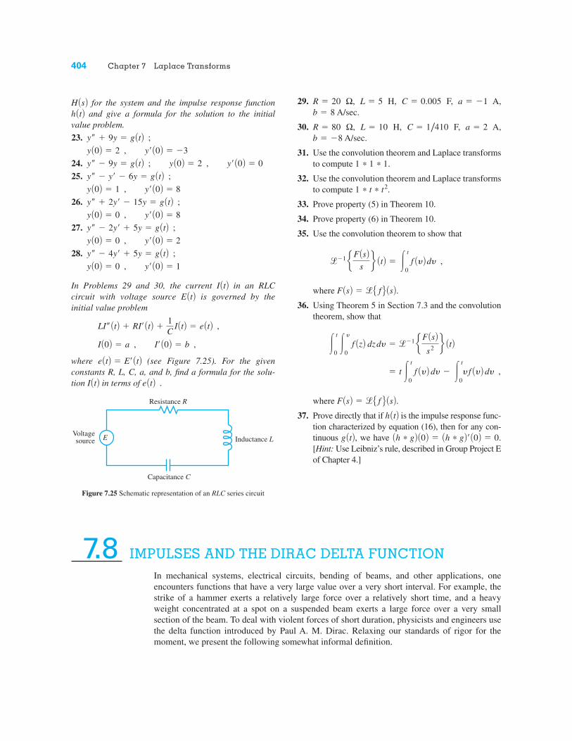
In Problems 29 and 30, the current in an RLCcircuit with voltage source is governed by theinitial value problem
where (see Figure 7.25). For the givenconstants R, L, C, a, and b, find a formula for the solu-tion in terms of e AtB .I AtB
e AtB " E¿ AtB I¿ A0B " b ,I A0B " a ,
LI– AtB ! RI¿ AtB !1C
I AtB " e AtB ,
E AtB I AtBy¿ A0B " 1y A0B " 0 , y– # 4y¿ ! 5y " g AtB ;
y¿ A0B " 2y A0B " 0 , y– # 2y¿ ! 5y " g AtB ;
y¿ A0B " 8y A0B " 0 , y– ! 2y¿ # 15y " g AtB ;
y¿ A0B " 8y A0B " 1 , y– # y¿ # 6y " g AtB ;
y¿ A0B " 0y A0B " 2 , y– # 9 y " g AtB ; y¿ A0B " #3y A0B " 2 ,
y– ! 9 y " g AtB ;
h AtBH AsB404 Chapter 7 Laplace Transforms
29. Ω, H, F, A,A/sec.
30. Ω, H, F, A,A/sec.
31. Use the convolution theorem and Laplace transformsto compute
32. Use the convolution theorem and Laplace transformsto compute
33. Prove property (5) in Theorem 10.
34. Prove property (6) in Theorem 10.
35. Use the convolution theorem to show that
where
36. Using Theorem 5 in Section 7.3 and the convolutiontheorem, show that
where
37. Prove directly that if is the impulse response func-tion characterized by equation (16), then for any con-tinuous we have "[Hint: Use Leibniz’s rule, described in Group Project Eof Chapter 4.]
Ah * gB ¿ A0B " 0.Ah * gB A0Bg AtB,h AtBF AsB " !E f F AsB. " t !
t
0 f AyB dy # !
t
0y f AyB dy ,
!t
0 !y
0 f AzB dz dy " !#1 e F AsB
s2 f AtBF AsB " !E f F AsB.
!#1 e F AsBsf AtB " !
t
0 f AyB dy ,
1 * t * t2.
1 * 1 * 1.
b " #8a " 2C " 1 /410L " 10R " 80
b " 8a " #1C " 0.005L " 5R " 20
E
Resistance R
Voltagesource
Capacitance C
Inductance L
Figure 7.25 Schematic representation of an RLC series circuit
7.8 IMPULSES AND THE DIRAC DELTA FUNCTIONIn mechanical systems, electrical circuits, bending of beams, and other applications, oneencounters functions that have a very large value over a very short interval. For example, thestrike of a hammer exerts a relatively large force over a relatively short time, and a heavyweight concentrated at a spot on a suspended beam exerts a large force over a very smallsection of the beam. To deal with violent forces of short duration, physicists and engineers usethe delta function introduced by Paul A. M. Dirac. Relaxing our standards of rigor for themoment, we present the following somewhat informal definition.
where is the Laplace transform of the solution to (12) with zero initial conditions and is the Laplace transform of It is important to note that and hence does notdepend on the choice of the function in (12) [see equation (15) in Section 7.7]. However, itis useful to think of the impulse response function as the solution of the symbolic initial valueproblem
(13)
Indeed, with we have and hence Consequently So we see that the function is the response to the impulse for a mechanical systemgoverned by the symbolic initial value problem (13).
d AtBh AtB h AtB ! y AtB.H AsB ! Y AsB.G AsB ! 1,g AtB ! d AtB,ay! " by# " cy $ D AtB ; y A0B $ 0 , y# A0B $ 0 .
g AtB h AtB,H AsB,g AtB. G AsBY AsB410 Chapter 7 Laplace Transforms
7.8 EXERCISES
In Problems 1–6, evaluate the given integral.
1.
2.
3.
4.
5.
6.
In Problems 7–12, determine the Laplace transform ofthe given generalized function.
7. 8.9. 10.
11. 12.
In Problems 13–20, solve the given symbolic initial valueproblem.13.
14.
15.y A0B ! 2 , y¿ A0B ! "2y– # 2y¿ " 3y ! d At " 1B " d At " 2B ;y A0B ! 1 , y¿ A0B ! 1y– # 2y¿ # 2y ! d At " pB ;w A0B ! 0 , w¿ A0B ! 0w– # w ! d At " pB ;
etd At " 3Bd At " pBsin tt3d At " 3Btd At " 1B 3d At " 1Bd At " 1B " d At " 3B
!1
"1Acos 2tBd AtB dt
!q
0e"2td At " 1B dt
!q
"qe"2td At # 1B dt
!q
"qAsin 3tBd at "
p
2bdt
!q
"qe3td AtB dt
!q
"qAt2 " 1Bd AtB dt
16.
17.
18.
19.
20.
In Problems 21–24, solve the given symbolic initial valueproblem and sketch a graph of the solution.21.
22.
23.
24.
In Problems 25–28, find the impulse response functionby using the fact that is the solution to the sym-
bolic initial value problem with and zero ini-tial conditions.25.26.27. 28. y– " y ! g AtBy– " 2y¿ # 5y ! g AtBy– " 6y¿ # 13y ! g AtBy– # 4y¿ # 8y ! g AtB
g AtB ! d AtBh AtBh AtBy A0B ! 0 , y¿ A0B ! 1y– # y ! d At " pB " d At " 2pB ;y A0B ! 0 , y¿ A0B ! 1y– # y ! "d At " pB # d At " 2pB ;y¿ A0B ! 1y A0B ! 0 , y– # y ! d At " p/2B ;
y¿ A0B ! 1y A0B ! 0 , y– # y ! d At " 2pB ;
y A0B ! 2 , y¿ A0B ! "5y– # 5y¿ # 6y ! e"td At " 2B ;w A0B ! 0 , w¿ A0B ! 4w– # 6w¿ # 5w ! etd At " 1B ;y¿ A0B ! 3y A0B ! 0 , y– " y¿ " 2y ! 3d At " 1B # et ;
y¿ A0B ! 2y A0B ! 0 , y– " y ! 4d At " 2B # t2 ; y A0B ! 2 , y¿ A0B ! 2y– " 2y¿ " 3y ! 2d At " 1B " d At " 3B ;
29. A mass attached to a spring is released from rest 1 mbelow the equilibrium position for the mass–springsystem and begins to vibrate. After sec, themass is struck by a hammer exerting an impulse onthe mass. The system is governed by the symbolicinitial value problem
where denotes the displacement from equilib-rium at time t. What happens to the mass after it isstruck?
30. You have probably heard that soldiers are told not tomarch in cadence when crossing a bridge. By solv-ing the symbolic initial value problem
explain why soldiers are so instructed. [Hint: SeeSection 4.10.]
31. A linear system is said to be stable if its impulseresponse function remains bounded as If the linear system is governed by
where b and c are not both zero, show that the systemis stable if and only if the real parts of the roots to
are less than or equal to zero.32. A linear system is said to be asymptotically stable
if its impulse response function satisfies asIf the linear system is governed by
show that the system is asymptotically stable if andonly if the real parts of the roots to
are strictly less than zero.33. The Dirac delta function may also be characterized
by the properties
and !q
"qd AtB dt ! 1 .
d AtB ! e 0 , t $ 0 ,
“infinite,” t ! 0 ,
ar 2 # br # c ! 0
ay– # by¿ # cy ! g AtB ,t S #q.h AtB S 0
ar 2 # br # c ! 0
ay– # by¿ # cy ! g AtB ,t S #q.h AtB
y¿ A0B ! 0 ,y A0B ! 0 ,
y– # y ! aq
k!1d At " 2kpB ;
x AtBdxdtA0B ! 0 ,x A0B ! 1 ,
d2xdt2 # 9x ! "3d at "
p
2b
p /2
Section 7.8 Impulses and the Dirac Delta Function 411
Formally using the mean value theorem for definiteintegrals, verify that if is continuous, then theabove properties imply
34. Formally using integration by parts, show that
Also show that, in general,
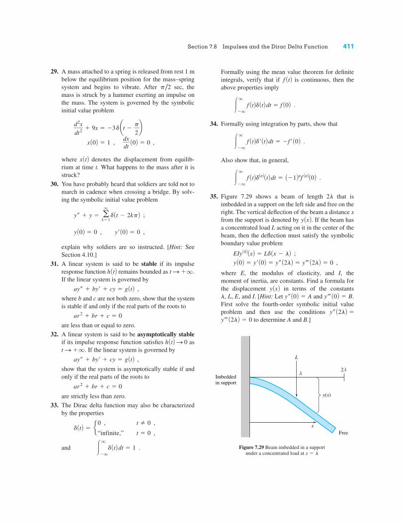
35. Figure 7.29 shows a beam of length that isimbedded in a support on the left side and free on theright. The vertical deflection of the beam a distance xfrom the support is denoted by If the beam hasa concentrated load L acting on it in the center of thebeam, then the deflection must satisfy the symbolicboundary value problem
where E, the modulus of elasticity, and I, themoment of inertia, are constants. Find a formula forthe displacement in terms of the constants
and I. [Hint: Let and First solve the fourth-order symbolic initial valueproblem and then use the conditions
to determine A and B.]y‡ A2lB ! 0y– A2lB !
y‡ A0B ! B.y– A0B ! Al, L, E,y AxB
y A0B ! y¿ A0B ! y– A2lB ! y‡ A2lB ! 0 ,EIy A4B AxB ! Ld Ax " lB ;
y AxB.2l
!q
"qf AtBdAnB AtB dt ! A"1Bnf AnB A0B .
!q
"qf AtBd¿ AtB dt ! "f ¿ A0B .
!q
"qf AtBd AtB dt ! f A0B .
f AtB
Imbeddedin support
L
2
y(x)
xFree
Figure 7.29 Beam imbedded in a support under a concentrated load at x ! l
To compute the inverse transform, we first write in the partial fraction form
Hence, from the Laplace transform table on the inside back cover, we find that
(4)
To determine we could solve system (3) for and then compute its inverse Laplacetransform. However, it is easier just to solve the first equation in system (1) for in terms of
Thus,
Substituting from equation (4), we find that
(5)
The solution to the initial value problem (1) consists of the pair of functions given byequations (4) and (5).
x AtB, y AtBy AtB ! "6e"4t # e2t " 2t .
x AtBy AtB !
12
x¿ AtB " 2t .
x AtB. y AtBY AsBy AtB,x AtB ! 3e"4t # e2t .
X AsB !3
s # 4#
1s " 2
.
X AsBSection 7.9 Solving Linear Systems with Laplace Transforms 413
7.9 EXERCISES
In Problems 1–19, use the method of Laplace transformsto solve the given initial value problem. Here etc.,denotes differentiation with respect to t; so does the sym-bol D.
1.
2.
3.
4.
5.
6.
7.
8. 4x # D 3 y 4 ! 3 ; y A0B ! 4
D 3 x 4 # y ! 0 ; x A0B ! 7 /4 ,
x " AD " 1B 3 y 4 ! 5e"3t ; y A0B ! 4
AD " 4B 3 x 4 # 6y ! 9e"3t ; x A0B ! "9 ,
"x # y¿ " y ! 0 ; y A0B ! "5 /2x¿ " x " y ! 1 ; x A0B ! 0 ,
y¿ ! x # 2 cos t ; y A0B ! 0x¿ ! y # sin t ; x A0B ! 2 ,
4x " y¿ " y ! cos t ; y A0B ! 0x¿ " 3x # 2y ! sin t ; x A0B ! 0 ,
z¿ " w¿ ! z " w ; w A0B ! 0z¿ # w¿ ! z " w ; z A0B ! 1 ,
y¿ ! 2x # 4y ; y A0B ! 0x¿ ! x " y ; x A0B ! "1 ,
y¿ ! 3y " 2x ; y A0B ! 1x¿ ! 3x " 2y ; x A0B ! 1 ,
x¿, y¿,9.
10.
11.
12.
13.
14.
15.
16.
17.x– " x¿ " 2y ! "et"2 ; x¿ A2B ! 1 , y A2B ! 1x¿ # x " y¿ ! 2 At " 2Bet"2 ; x A2B ! 0 ,
2x # y¿ # y ! sin t # 3 cos t ; y ApB ! 3
x¿ " 2x # y¿ ! " Acos t # 4 sin tB ; x ApB ! 0 ,
x¿ # x " y¿ ! t2 # 2t " 1 ; y A1B ! 0
x¿ " 2y ! 2 ; x A1B ! 1 ,
y¿ A0B ! 0
y– ! x # 1 " u At " 1B ; y A0B ! 0 ,
x¿ A0B ! 0 ,x– ! y # u At " 1B ; x A0B ! 1 ,
x # y¿ ! 0 ; y A0B ! 1
x¿ " y¿ ! Asin tBu At " pB ; x A0B ! 1 ,
2x¿ # y– ! u At " 3B ; y¿ A0B ! "1
x¿ # y ! x ; x A0B ! 0 , y A0B ! 1 ,
x # y¿ ! 0 ; y A0B ! 0
x¿ # y ! 1 " u At " 2B ; x A0B ! 0 ,
y¿ A0B ! "1x # y– ! "1 ; y A0B ! 1 , x¿ A0B ! 1 ,x– # y ! 1 ; x A0B ! 1 ,
"3x– # 2y– ! 3x " 4y ; y A0B ! 4 , y¿ A0B ! "9x– # 2y¿ ! "x ; x A0B ! 2 , x¿ A0B ! "7 ,
The use of the Laplace transform helps to simplify the process of solving initial value problemsfor certain differential and integral equations, especially when a forcing function with jumpdiscontinuities is involved. The Laplace transform of a function is defined by
for all values of s for which the improper integral exists. If is piecewise continuous onand of exponential order [that is, grows no faster than a constant times as
], then exists for all The Laplace transform can be interpreted as an integral operator that maps a function
to a function The transforms of commonly occurring functions appear in Table 7.1, page 359,F AsB. f AtBs 7 a.!E f F AsBt S qeat0 f AtB 0a30, q B f AtB
!E f F AsB J !q
0 e!stf AtB dt
f AtB!E f F
18.
19.
20. Use the method of Laplace transforms to solve
[Hint: Let and then solve for c.]21. For the interconnected tanks problem of Section 5.1,
page 242, suppose that the input to tank A is nowcontrolled by a valve which for the first 5 min deliv-ers 6 L/min of pure water, but thereafter delivers 6L/min of brine at a concentration of 2 kg/L. Assumingthat all other data remain the same (see Figure 5.1,page 242), determine the mass of salt in each tank for t $ 0 if and .
22. Recompute the coupled mass–spring oscillatormotion in Problem 1, Exercises 5.6 (page 289),using Laplace transforms.
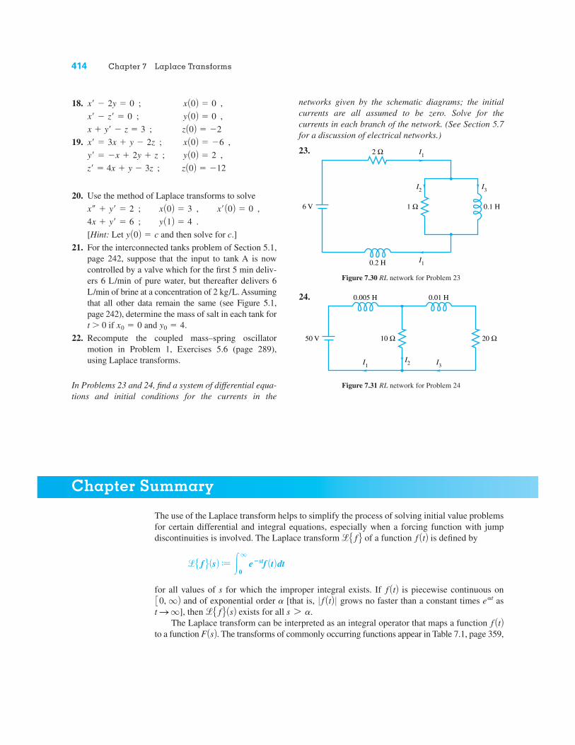
In Problems 23 and 24, find a system of differential equa-tions and initial conditions for the currents in the
y0 ! 4x0 ! 0
y A0B ! c 4x # y¿ ! 6 ; y A1B ! 4 . x– # y¿ ! 2 ; x A0B ! 3 , x¿ A0B ! 0 ,
z¿ ! 4x # y " 3z ; z A0B ! "12y¿ ! "x # 2y # z ; y A0B ! 2 ,x¿ ! 3x # y " 2z ; x A0B ! "6 ,x # y¿ " z ! 3 ; z A0B ! "2x¿ " z¿ ! 0 ; y A0B ! 0 ,x¿ " 2y ! 0 ; x A0B ! 0 ,
414 Chapter 7 Laplace Transforms
networks given by the schematic diagrams; the initialcurrents are all assumed to be zero. Solve for thecurrents in each branch of the network. (See Section 5.7for a discussion of electrical networks.)
6 V
2 Ω
I2 I3
I1
I1
1 Ω
0.2 H
0.1 H
Figure 7.30 RL network for Problem 23
23.
50 V
I1 I3I2
20 Ω10 Ω
0.005 H 0.01 H
Figure 7.31 RL network for Problem 24
24.
Chapter Summary
method. For this purpose, the rectangular window function isuseful. The transform of a periodic forcing function with period T is given by
The Dirac delta function is useful in modeling a system that is excited by a large forceapplied over a short time interval. It is not a function in the usual sense but can be roughlyinterpreted as the derivative of a unit step function. The transform of is
!Ed At ! aB F AsB " e!as , a # 0 .
d At ! aBd AtB!E f F AsB "
!T
0e!stf AtB dt
1 ! e!sT .
f AtB ßa,b AtB " u At ! aB ! u At ! bB416 Chapter 7 Laplace Transforms
REVIEW PROBLEMS
In Problems 1 and 2, use the definition of the Laplacetransform to determine .
1.
2.
In Problems 3–10, determine the Laplace transform ofthe given function.
3. 4.5.6.7.8. 9.
10. and has period p.
In Problems 11–17, determine the inverse Laplace trans-form of the given function.
11. 12.
13.
14.
15. 16.
17.e!2s A4s $ 2BAs ! 1B As $ 2B
1As2 $ 9B22s2 $ 3s ! 1As $ 1B2 As $ 2Bs2 $ 16s $ 9As $ 1B As $ 3B As ! 2B
4s2 $ 13s $ 19As ! 1B As2 $ 4s $ 13B2s ! 1
s2 ! 4s $ 67As $ 3B3
f AtBf AtB " cos t, !p/2 % t % p/2t2u At ! 4BAt $ 3B2 ! Aet $ 3B2t cos 6t
7e2t cos 3t ! 2e7t sin 5te2t ! t3 $ t2 ! sin 5t
e3t sin 4tt2e!9t
f AtB " e e!t , 0 % t % 5 ,
!1 , 5 6 t
f AtB " e 3 , 0 % t % 2 ,
6 ! t , 2 6 t
!E f F 18. Find the Taylor series for about t " 0.Then, assuming that the Laplace transform of can be computed term by term, find an expansion for
in powers of .
In Problems 19–24, solve the given initial value problemfor using the method of Laplace transforms.
19.
20.
21.
22.
23.
24.
In Problems 25 and 26, find solutions to the given initialvalue problem.
25.
26.
y A0B " 1 , y¿ A0B " !1
ty– $ 2 At ! 1By¿ $ At ! 2By " 0 ;
y¿ A0B " 0y A0B " 0 , ty– $ 2 At ! 1By¿ ! 2y " 0 ;
y¿ A0B " 0y A0B " 0 , y– ! 4y¿ $ 4y " t2et ;
y¿ A0B " 1y A0B " 0 , y– $ 3y¿ $ 4y " u At ! 1B ;
y¿ A0B " 5y A0B " !1 , y– $ 9y " 10e2t ; y A0B " 0 , y¿ A0B " !1
y– $ 2y¿ $ 2y " t2 $ 4t ;
y¿ A0B " 10y A0B " !3 , y– $ 6y¿ $ 9y " 0 ;
y¿ A0B " !3y A0B " 0 , y– ! 7y¿ $ 10y " 0 ;
y AtB1 /s!E f F AsB f AtBf AtB " e!t2
In Problems 27 and 28, solve the given equation for
27.
28.
29. A linear system is governed by
Find the transfer function and the impulse responsefunction.
y– ! 5y¿ $ 6y " g AtB .y A0B " !1
y¿ AtB ! 2 !t
0y AyBsin At ! yB dy " 1 ;
y AtB $ !t
0At ! yBy AyB dy " e!3t
y AtB.Technical Writing Exercises 417
TECHNICAL WRITING EXERCISES
30. Solve the symbolic initial value problem
In Problems 31 and 32, use Laplace transforms to solvethe given system.31.
32.y A0B " 0x $ y¿ " y ;
x– $ 2y¿ " u At ! 3B ; x A0B " 1 , x ¿A0B " !1 ,x $ y¿ " 1 ! u At ! 2B ; y A0B " 0x¿ $ y " 0 ; x A0B " 0 ,
y A0B " 0 , y¿ A0B " 1 .
y– $ 4y " d at !p2b ;
1. Compare the use of Laplace transforms in solvinglinear differential equations with constant coeffi-cients with the use of logarithms in solving algebraicequations of the form
2. Explain why the method of Laplace transformsworks so well for linear differential equations withconstant coefficients and integro-differential equa-tions involving a convolution.
3. Discuss several examples of initial value problemsin which the method of Laplace transforms cannotbe applied.
xr " a.
4. A linear system is said to be asymptotically stable ifits impulse response function as Assume the Laplace transform of is arational function in reduced form with the degree ofits numerator less than the degree of its denominator.Explain in detail how the asymptotic stability of thelinear system can be characterized in terms of thezeros of the denominator of Give examples.
5. Compare and contrast the solution of initial valueproblems by Laplace transforms versus the methodsof Chapter 4.
H AsB.
h AtB,H AsB, t S $q.h AtB S 0