Chapter 5 –Compilers - Maniramanathaenggnotebook.weebly.com/.../chapter_5compilersnew.pdf · Chapter 5 – Compilers ... grammar. This grammar specifies the form, ... z After the

System Software – An Introduction to Systems Programming, 3rd ed., Leland L. Beck

Chapter 5 – Compilers 5.1 Basic Compiler Functions

Fig 5.1 shows an example Pascal program for the following explanations.

For the purposes of compiler construction, a high-level

programming language is usually described in terms of grammar. This grammar specifies the form, or syntax, of legal statements in the language. The problem of compilation then becomes one of matching statements written by the programmer to structures defined by the grammar, and generating the

Written by WWF １


Written by WWF ２

appropriate object code for each statement. A source program statement can be regarded as a

sequence of tokens rather than simply as a string of characters. Tokens may be thought of as the fundamental building blocks of the language. For example, a token might be a keyword, a variable name, an integer, an arithmetic operator, etc.

The task of scanning the source statement, recognizing and classifying the various tokens, is known as lexical analysis. The part of the compiler that performs this analytic function is commonly called the scanner.

After the token scan, each statement in the program must be recognized as some language construct, such as a declaration or an assignment statement, described by the grammar. This process, called syntactic analysis or parsing, is performed by a part of the compiler that is usually called the parser.

The last step in the basic translation process is the generation of object code. Most compilers create machine-language programs directly instead of producing a symbolic program for later translation by an assembler.

Although we have mentioned three steps in the compilation process – scanning, parsing, and code generation – it is important to realize that a compiler does not necessarily make three passes over the program being translated. For some languages, it is quite possible to compile a program in a single pass.


Written by WWF ３

5.1.1 Grammars A grammar for a programming language is a formal

description of the syntax, or form, of programs and individual statements written in the language.

The grammar does not describe the semantics, or meaning, of the various statements; such knowledge must be supplied in the code-generation routines. Example: for the difference between syntax and semantics, consider the two statements (I := J + K) and (X := Y + I), where X and Y are REAL variables and I, J, K are INTEGER variables. These two statements have identical syntax. However, the semantics of the two statements are quite different. The first statement specifies that the variables in the expression are to be added using integer arithmetic operations. The second statement specifies a floating-point addition, with the integer operand I being converted to floating point before adding.

Obviously, these two statements would be compiled into very different sequences of machine instructions. However, they would be described in the same way by the grammar. The differences between the statements would be recognized during code generation.

A number of different notations can be used for writing grammars. The one we describe is called BNF (for Backus-Naur Form). Fig 5.2 gives one possible BNF grammar for a highly restricted subset of Pascal.


A BNF grammar consists of a set of rules, each of which

defines the syntax of some construct in the programming language. For example, Rule 13 in Fig 5.2: <read> ::= READ ( <id-list> ). This is a definition of the syntax of a Pascal READ statement that is denoted in the grammar as <read>. The symbol ::= can be read “is defined to be”. On the left of this symbol is the language construct being defined, <read>, and on the right is a description of the syntax being defined for it.

Character strings enclosed between the angle brackets < and > are called nonterminal symbols (such as ‘<read>’ and ‘<id-list>’). These are the names of constructs defined in the grammar. Entries not enclosed in angle brackets are terminal symbols of the grammar (i.e., tokens, such as ‘READ’, ‘(‘, and ‘)’). The blank spaces in the grammar rules are not significant.

Written by WWF ４


They have been included only to improve readability. To recognize a <read> (to resolve all nonterminal

symbols), we also need the definition of <id-list>. This is provided by Rule 6 in Fig 5.2. <id-list> ::= id | <id-list>, id This rule offers two possibilities, separated by the | symbol, for the syntax of an <id-list>. The first alternative specifies that an <id-list> may consist simply of a token id (the notation id denotes an identifier that is recognized by the scanner). The second alternative is an <id-list>, followed by the token “,” (comma), followed by a token id. Example: ALPHA is an <id-list> that consists of a single id ALPHA; ALPHA , BETA is an <id-list> that consists of another <id-list> ALPHA, followed by a comma, followed by an id BETA, and so forth.

It is often convenient to display the analysis of a source statement in terms of a grammar as a tree. This tree is usually called the parse tree, or syntax tree, for the statement. Fig 5.3(a) shows the parse tree for the statement READ ( VALUE ).

Written by WWF ５


Rule 9 of the grammar in Fig 5.2 provides a definition of the syntax of an assignment statement: <assign> ::= id := <exp> That is, an <assign> consists of an id, followed by the token :=, followed by an expression <exp>.

Rule 10 gives a definition of an <exp>: <exp> ::= <term> | <exp> + <term> | <exp> - <term>

Continuously, Rule 11 defines a <term> to be any sequence of <factor>s connected by * and DIV.

Again, Rule 12 specifies that a <factor> may consist of an identifier id or an integer int (which is also recognized by the scanner) or an <exp> enclosed in parentheses.

Fig 5.3(b) shows the parse tree for statement 14 from Fig 5.1 in terms of the rules just described.

Written by WWF ６


Note that the parse tree in Fig 5.3(b) implies that multiplication and division are done before addition and subtraction (that is, multiplication and division have higher precedence than addition and subtraction). The terms SUMSQ DIV 100 and MEAN * MEAN must be calculated first since these intermediate results are the operands (left and right subtrees) for the – operation.

The parse trees shown in Fig 5.3 represent the only possible ways to analyze these two statements in terms of the grammar of Fig 5.2. If there is more than one possible parse tree for a given statement, the grammar is said to be ambiguous.

Fig 5.4 shows the parse tree for the entire program in Fig 5.1.

Written by WWF ７


5.1.2 Lexical Analysis

Lexical analysis involves scanning the program to be compiled and recognizing the tokens that make up the source statements. Scanners are usually designed to recognize keywords, operators, and identifiers, as well as integers, floating-point numbers, character strings, and other similar items.

Items such as identifiers and integers are usually recognized directly as single tokens and might be defined as a part of the grammar. For example, <ident> ::= <letter> | <ident> <letter> | <ident> <digit> <letter> ::= A | B | C | … | Z <digit> ::= 0 | 1 | …| 9

The output of the scanner consists of a sequence of tokens. For efficiency of later use, each token is usually represented by some fixed-length code, such as an integer, rather than as a variable-length character string.

Written by WWF ８


In such a token coding scheme for the grammar of Fig 5.2 (shown in Fig 5.5), the token PROGRAM would be represented by the integer value 1, an identifier id would be represented by the value 22, and so on.

When the token being scanned is a keyword or an

operator, such a coding scheme gives sufficient information. However, in the case of identifier, it is also necessary to specify the particular identifier name that was scanned. The same is true for integers, floating-point values, character-string constants, etc. This can be accomplished by associating a token specifier with the type code for such tokens. The specifier gives the identifier name, integer value, etc., that was found by the scanner.

Written by WWF ９


Fig 5.6 shows the output from a scanner for the program in Fig 5.1, using the token coding scheme in Fig 5.5.

For token type 22 (identifier), the token specifier is a pointer to a symbol-table entry (denoted be ^SUM, ^SUMSQ, etc.). For token type 23 (integer), the specifier is the value of the integer (denoted by #0, #100, etc.).

The scanner usually is responsible for reading the lines of the source program as needed, and possibly for printing

Written by WWF １０


Written by WWF １１

the source listing. Comments are ignored by the scanner, except for printing on the output listing.

The process of lexical scanning is quite simple. However, many languages have special characteristics that must be considered when programming a scanner. For example, in FORTRAN, a number in columns 1-5 of a source statement should be interpreted as a statement number, not as an integer.

Languages that do not have reserved words create even more difficulties for the scanner. For example, in FORTRAN, any keyword may also be used as an identifier (See the case in the lower part of page 237). In such a case, the scanner might interact with the parser so that it could tell the proper interpretation of each word, or it might simply place identifiers and keywords in the same class, leaving the task of distinguishing between them to the parser.

Modeling Scanners as Finite Automata The tokens of most programming languages can be

recognized by a finite automaton. Finite automata are often represented graphically, as illustrated in Fig 5.7(a). States are represented by circles, and transitions by arrows from one state to another. Each arrow is labeled with a character or a set of characters that cause the specified transition to occur.

Consider, for example, the finite automaton shown in Fig 5.7(a) and the first input string in Fig 5.7(b).


The automaton starts in State 1 and examines the first character of the input string. The character α causes the automaton to move from State 1 to State 2. The b causes a transition from State 2 to State 3, etc.

The first two input strings in Fig 5.7(b) can be recognized by the finite automaton in Fig 5.7(a). Consider the third input string in Fig 5.7(b). The finite automaton beings in State 1, as before, and the α causes a transition from State 1 to State 2. Now the next character to be scanned is c. However, there is no transition from State 2 that is labeled with c. Therefore, the automaton must stop in State 2.

Fig 5.8 shows several finite automata that are designed to recognize typical programming language tokens.

Written by WWF １２


Fig 5.8(a) recognizes identifiers and keywords that begin with a letter and may continue with any sequence of letters and digits. Some languages allow identifiers such as NEXT_LINE, which contains the underscore character (_). Fig 5.8(b) shows a finite automaton that recognizes identifiers of this type.

Written by WWF １３


The finite automaton in Fig 5.8(c) recognizes integers that consist of a string of digits, including those that contain leading zeroes, such as 000025. Fig 5.8(d) shows an automaton that does not allow leading zeroes, except in the case of the integer 0.

Each of the finite automata we have seen so far was designed to recognize one particular type of token. Fig 5.9 shows a finite automaton that can recognize all of the tokens listed in Fig 5.5.

In Fig 5.9, a special case occurs in State 3. Suppose that the scanner encounters an erroneous token such as “VAR.”.

When the automaton stops in State 3, the scanner should perform a check to see whether the string being recognized is “END.”. If it is not, the scanner could back up to State 2 (recognizing the “VAR”). The period would then be

Written by WWF １４


rescanned as part of the following token the next time the scanner is called.

Finite automata provide an easy way to visualize the operation of a scanner. Fig 5.10(a) shows a typical algorithm to recognize such a token. Fig 5.10(b) shows the finite automaton from Fig 5.8(b) represented in a tabular form.

Written by WWF １５


Written by WWF １６

5.1.3 Syntactic Analysis During syntactic analysis, the source statements written

by the programmer are recognized as language constructs described by the grammar being used.

We may think of this process as building the parse tree for the statements. Parsing techniques are divided into two general classes – bottom-up and top-down – according to the way in which the parse tree is constructed. Top-down methods (ex. recursive-descent parsing) begin with the rule of the grammar that specifies the goal of the analysis (i.e., the root of the tree), and attempt to construct the tree so that the terminal nodes match the statements being analyzed. Bottom-up methods (ex. operator-precedence parsing) begin with the terminal nodes of the tree (the statements being analyzed), and attempt to combine these into successively higher-level nodes until the root is reached.

A large number of different parsing techniques have been devised, most of which are applicable only to grammars that satisfy certain condition.

Operator-Precedence Parsing The bottom-up parsing technique we consider is called

the operator precedence method. This method is based on examining pairs of consecutive operators in the source program, and making decisions about which operation should be performed first. For example, the arithmetic expression “A + B * C – D”. According to usual rules of arithmetic, * and / have higher precedence than + and –. If we examine the first two operators + and *, we find that + has lower precedence than *. This is often written as “+ < *”.


Written by WWF １７

Similarly, for the next part pair of operators * and –, we would find that * has higher precedence than –. We may write this as “* > –”.

A + B * C – D

< >

This implies that the subexpression B*C is to be computed before either of the other operations in the expression is performed.

The first step in constructing an operator-precedence parser is to determine the precedence relations between the operators of the grammar. In this context, operator is taken to mean any terminal symbol (i.e., any token), so we also have precedence relations involving tokens such as BEGIN, READ, id, etc. The matrix in Fig 5.11 shows these precedence relations for the grammar in Fig 5.2.


The relation ≐ indicates that the two tokens involved have equal precedence and should be recognized by the parser as part of the same language construct.

Note that the precedence relations do not follow the ordinary rules for comparisons. For example, we have “; > END” but “END > ;”. That is, when ; is followed by END, the ; has higher

precedence. But when END is followed by ;, the END has higher

Written by WWF １８


precedence. Also note that in many cases, there is no precedence

relation between a pair of tokens. This means that these two tokens cannot appear together in any legal statement. If such a combination occurs during parsing, it should be recognized as a syntax error.

There are algorithmic methods for constructing a precedence matrix like Fig 5.11 from a grammar [see, for example, Aho et al. (1998)]. For the operator-precedence parsing method to be applied, it is necessary that all the precedence relations be unique.

Fig 5.12 shows the application of the operator-precedence parsing method to the READ statement from line 9 of the program in Fig 5.1.

The statement is scanned from left to right, one token at a time. For each pair of operators, the precedence relation between them is determined. Part (ii) of Fig 5.12 shows the statement being analyzed

Written by WWF １９


Written by WWF ２０

with id replaced by <N1>.

Part (ii) of Fig 5.12 also shows the precedence relations that hold in the new version of the statement. An operator-precedence parser generally uses a stack to save tokens that have been scanned but yet parsed, so it can reexamine them in this way. Precedence relations hold only between terminal symbols, so <N1> is not involved in this process, and a relationship is determined between ( and ).

Fig 5.13 shows a similar step-by-step parsing of the assignment statement from line 14 of the program in Fig 5.1.


Written by WWF ２１


Note that the left-to-right scan is continued in each step only far enough to determine the next portion of the statement to be recognized, which is the first portion delimited by < and >. Once this portion has been determined, it is interpreted as a nonterminal according to some rule of the grammar.

This process continues until the complete statement is recognized. Note that (see Fig 5.13) each portion of the parse tree is constructed from the terminal nodes up toward the root, hence the term bottom-up parsing. Although we have illustrated operator-precedence

Written by WWF ２２


Written by WWF ２３

parsing only on single statements, the same techniques can be applied to an entire program.

Behind the operator precedence technique, a more general method known as shift-reduce parsing was developed. Shift-reduce parsers make use of a stack to store tokens that have not yet been recognized in terms of the grammar. The actions of the parser are controlled by entries in a table, somewhat similar to the precedence matrix discussed before. The two main actions are shift (push the current token onto the stack) and reduce (recognize symbols on top of the stack according to a rule of the grammar).

Fig 5.14 illustrates this shift-reduce process, using the same READ statement considered in Fig 5.12. The token currently being examined by the parser is indicated by ↑.


In Fig 5.14(a), the parser shifts (pushing the currently token onto the stack) when it encounters the token BEGIN.

Written by WWF ２４


Written by WWF ２５

In Fig 5.14 (b-d), similar to the action in Fig 5.14(a). In Fig 5.14(e), when parser examines the token ), the reduce action is invoked. A set of tokens from the top of the stack (in this case, the single token id) is reduced to a nonterminal symbol from the grammar (in this case, <id-list>). In Fig 5.14(f), the token ) is considered again. This time, it will be pushed onto the stack, to be reduced later as part of the READ statement.

For this simple type of grammar, shift roughly corresponds to the action taken by an operator-precedence parser when it encounters the relations < and ≐. Reduce roughly corresponds to the action taken when an operator-precedence parser encounters the relation >.

Recursive-Descent Parsing The other parsing technique is a top-down method known

as recursive descent. A recursive descent parser is made up of a procedure for each nonterminal symbol.

As an example for illustrating the parsing process of a recursive descent parser, consider Rule 13 of the grammar in Fig 5.2. The procedure for <read> in a recursive-decent parser first examines the next two input tokens, looking for READ and (. If these are found, the procedure for <read> then calls the procedure for <id-list>. If that procedure (for <id-list>) succeeds, the <read> procedure examines the next input token, looking for ). If all these tests are successful, the <read> procedure


Written by WWF ２６

returns an indication of success to its caller and advances to the next token following ). Otherwise, the <read> procedure returns an indication of

failure. When there are several alternatives defined by the

grammar for a nonterminal, the procedure is only slightly more complicated. For the recursive-descent technique, it must be possible to decide which alternative to use by examining the next input token. For example, the procedure for <stmt> looks at the next token to decide which of its four alternatives to try. If the token is READ, it calls the procedure for <read>; if the token is id, it calls the procedure for <assign> because this is the only alternative that can begin with the token id, and so on.

There is a problem. For example, the procedure for <id-list>, corresponding to Rule 6, would be unable to decide between its two alternatives since id and <id-list> can begin with id. If the procedure decided to try the 2nd alternative (<id-list>, id), it would immediately call itself recursively to find an <id-list>. This could result in another immediate recursive call, which leads to an unending chain. The reason for this is that one of the alternatives for <id-list> begins with <id-list>. Therefore, top-down parsers cannot be directly used with a grammar that contains this kind of immediate left recursion.

Fig 5.15 shows the grammar from Fig 5.2 with left recursion eliminated.


Top-down parsing using new grammar: Consider Rule 6a

in Fig 5.15. This notation specifies that the terms between {and} may be omitted, or repeated one or more times. Thus, Rule 6a defines <id-list> as being composed of an id followed by zero or more occurrences of “, id”. This is clearly equivalent to Rule 6 of Fig 5.2.

Fig 5.16 illustrates a recursive-descent parse of the READ statement on line 9 of Fig 5.1, using the grammar in Fig 5.15.

Written by WWF ２７


Written by WWF ２８


Written by WWF ２９

Fig 5.16(a) shows the procedures for the nonterminals <read> and <id-list>. Assume that the variable TOKEN contains the type of the next input token, using the coding scheme shown in Fig 5.5.

Fig 5.16(b) (corresponding to the algorithms in Fig 5.16(a)) gives a graphic representation of the recursive-descent parsing process for the statement being analyzed. In part (i), the READ procedure has been invoked and has examined the tokens READ and ( from the input stream (indicated by the dashed lines). In part (ii), READ has called IDLIST (indicated by the solid line), which has examined the token id. In part (iii), IDLIST has returned to READ, indicating success; READ has then examined the input token ). This completes the analysis of the source statement. The procedure READ will now return to its caller, indicating that a <read> was successfully found.

Fig 5.17 illustrates a recursive-descent parse of the assignment statement on line 14 of Fig 5.1.


Written by WWF ３０


Written by WWF ３１


Fig 5.17(a) shows the procedures (ASSIGN, EXP, TERM, FACTOR) for the nonterminal symbols that are involved in parsing this statement. You should carefully compare these procedures to the corresponding rules of the grammar. Fig 5.17(b) is a step-by-step representation of the procedure calls and token examinations similar to that shown in Fig 5.16(b).

Written by WWF ３２

Note that the same technique can be applied to an entire program.


Written by WWF ３３

5.1.4 Code Generation The code-generation technique we describe involves a

set of routines, one for each rule or alternative rule in the grammar. When the parser recognizes a portion of the source program according to the some rule of the grammar, the corresponding routine is executed. Such routines are often called semantic routines.

Note that code-generation techniques need not be associated with any particular parsing method.

Assume that our code-generation routines make use of two data structures for working storage: a list and a stack. Items inserted into the list are removed in the order of their insertion, first-in-first-out. Items pushed onto the stack are removed (popped from the stack) in the opposite order, last-in-first-out. In addition, LISTCOUNT is used to keep a count of the number of items currently in the list. The code-generation routines also make use of the token specifiers; these specifiers are denoted by S(token). For a token id, S(id) is the name of the identifier, or a pointer to the symbol-table entry for it.

Fig 5.18 illustrates the application of our code-generation process to the READ statement of line 9 of the program in Fig 5.1. The parse tree for this statement is repeated for convenience in Fig 5.18(a).


Fig 5.18(c) shows a symbolic representation of the object code to be generated for the READ statement. This code consists of a call to a subroutine XREAD, which would be part of a standard library associated with the compiler.

Written by WWF ３４


Written by WWF ３５

Since XREAD may be used to perform any READ operation, it must be passed parameters that specify the details of the READ. In this case, the parameter list for XREAD is defined immediately after the JSUB that call it. Thus, the 2nd line in Fig 5.18(c) specifies that one variable is to be read (WORD 1), and the 3rd line gives the address of this variable.

Fig 5.18(b) shows a set of routines that might be used to accomplish this code generation. The first two routines correspond to alternative structures for <id-list>, which are shown in Rule 6 of the grammar in Fig 5.2. In either case, the token specifier S(id) for a new identifier being added to the <id-list> is inserted into the list used by the code-generation routines, and LISTCOUNT is updated to reflect this insertion. After the entire <id-list> has been parsed, the list contains the token specifiers for all the identifiers that are part of the <id-list>. When the <read> statement is recognized, these token specifiers are removed from the list and used to generate the object code for the READ. (See code generation routine <read> in Fig 5.18(b) in page 262.)

Remember that, in generating the tree shown in Fig 5.18(a), recognizes first <id-list> and then <read>. At each step, the parser calls the appropriate code-generation routine.

Fig 5.19 shows the code-generation process for the assignment statement on line 14 of Fig 5.1.


Written by WWF ３６


Written by WWF ３７


Fig 5.19(a) displays the parse tree for this statement. Most of the work of parsing involves the analysis of the <exp> on the right-hand side of the :=.

Written by WWF ３８


Written by WWF ３９

The parser first recognizes the id SUMSQ as a <factor> and a <term>. Then it recognizes the int 100 as a <factor>. Then it recognizes SUMSQ DIV 100 as a <term>, and so

forth. Note that the order of parsing the statement is the same as the order of arithmetic evaluation.

As each portion of the statement is recognized, a code-generation routine is called to create the corresponds object code. For example, suppose we want generate code that corresponds to the rule <term>1 ::= <term>2 * <factor>.

Our code-generation routines perform all arithmetic operations using register A, so we clearly need to generate a MUL instruction in the object code. The result of this multiplication, <term>1, will be left in register A by the MUL. If either <term>2 or <factor> is already present in register A, perhaps as the result of a previous computation, the MUL instruction is all we need. Otherwise, we must generate a LDA instruction preceding the MUL. In this case, the previous value in register A must be saved (store somewhere) if it will be required for later use.

Obviously, we need to keep track of the result left in register A by each segment of code that is generated. In the example just discussed, the node specifier S(<term>1) would be set to rA, indicating that the result of this computation is in register A.


Written by WWF ４０

The variable REGA is used to indicate the highest-level node of the parse tree whose value is left in register A by the code generated so far (i.e., the node whose specifier is rA)

As an illustration of these ideas, consider again the code- generation routine in Fig 5.19(b) that corresponds to the rule <term>1 ::= <term>2 * <factor>

If the node specifier for either operand is rA, the corresponding value is already in register A, so the routine simply generates a MUL instruction. The operand address for this MUL is given by the node specifier for the other operand (the one not in the register). Otherwise, the procedure GETA (shown in Fig 5.19(c)) is called. This procedure generates a LDA instruction to load the value associated with <term>2 into register A.

However, before the LDA, the procedure generates a STA instruction to save the value currently in register A. After the necessary instructions are generated, the code- generation routine sets S(<term>1) and REGA to indicate that the value corresponding to <term>1 is now in register A. This completes the code-generation actions for the * operation.

The code-generation routine that corresponding to the “+” operation is almost identical to the one just discussed for *. The routines for DIV and – are similar, except that for these operations, it is necessary for the first operand to be in register A.

The code generation for <assign> consists of bringing the


Written by WWF ４１

value to be assigned into register A (using REGA) and then generating a STA instruction. Note that REGA is then set to null.

Fig 5.19(d) shows a symbolic representation of the object code generated for the assignment statement being translated.

Fig 5.20 shows the other code-generation routines for the grammar in Fig 5.2. The routine for <prog-name> generates header information in the object program that is similar to that created from the START and EXTREF assembler directives.


Written by WWF ４２


It also generates instructions to save the return address and jump to the first executable instruction in the compiled program.

Written by WWF ４３


The compiler also generates any Modification records required to describe external references to library subroutines.

For the complete code-generation process of the program in Fig 5.1, it is shown in Fig 5.21.

Written by WWF ４４


Written by WWF ４５

5.2 Machine-Dependent Compiler Features

The process of analyzing the syntax of programs written in high-level languages should be relatively machine-independent. The real machine dependencies of a compiler are related to the generation and optimization of the object code.

There are many complex issues involving the code generation such as the allocation of registers and the rearrangement of machine instructions to improve efficiency of execution. Such types of code optimization are normally done by considering an intermediate form of the program being compiled. In this intermediate form, the syntax and semantics of the source statements have been completely analyzed, but the actual translation into machine code has not yet been performed.

For the purposes of code optimization, the intermediate form of the program is much easier to analyze and manipulate than in either the source program or the machine code.

5.2.1 Intermediate Form of the Program There are many possible ways of representing a program

(in Aho et al., 1988) in an intermediate form for code analysis and optimization. The intermediate form used is a sequence of quadruples below. operation, op1, op2, result where operation is some function to be performed by the object code, op1 and op2 are the operands for this


Written by WWF ４６

operation, and result designates where the resulting value is to be placed.

Example 1: “SUM := SUM + VALUE“ could be represented with the quadruples

+ , SUM, VALUE, i1 := , i1 , , SUM

Example 2: “VARIANCE := SUMSQ DIV 100 – MEAN * MEAN” could be represented with the quadruples

DIV, SUMSQ, #100 , i1 * , MEAN , MEAN, i2 ﹣ , i1 , i2 , i3 := , i3 , , VARIANCE

The above quadruples would be created by intermediate code-generation routines similar to those discussed in Section 5.1.4.

Many types of analysis and manipulation can be performed on the quadruples for code-optimization purposes. For example, the quadruples can be rearranged to eliminate redundant load and store operations, and the intermediate results ij can be assigned to registers or to temporary variables to make their use as efficient as possible. After optimization has been performed, the modified quadruples are translated into machine code.

Fig 5.22 shows a sequence of quadruples corresponding to the source program in Fig 5.1.


5.2.2 Machine-Dependent Code Optimization

To perform machine-dependent code optimization, the first problem is the assignment and use of registers.

On many computers, there are a number of general-purpose registers that may be used to hold some useful data. Machine instructions that use registers as operands are usually faster than the corresponding instructions that refer to locations in memory. Therefore, we would prefer to keep in registers all variables and intermediate results that will be used later in the program. For example, consider the quadruples shown in Fig 5.22.

Written by WWF ４７


Written by WWF ４８

The variable VALUE is used once in quadruple 7 and twice in quadruple 9. If registers are enough and available, it would be possible to fetch this value only once.

Note that there are rarely as many registers available as we would like to use. The problem then becomes one of selecting which register value to replace when it is necessary to assign a register for some other purpose. One reason approach is to scan the program for the next point at which each register value would be used. The value that will not be needed for the longest time is the one that should be replaced.

In making and using register assignments, a compiler must also consider the control flow of the program. The existence of Jump instructions creates difficulty in keeping track of register contents. One way to deal with this problem is to divide the program into basic blocks. A basic block is a sequence of quadruples with one entry point, which is at the beginning of the block, one exit point, which at end of the block, and no jumps within the block.

Since procedure calls can have unpredictable effects on register contents, a CALL operation is also usually considered to begin a new basic block.

Fig 5.23 shows the division of the quadruples from Fig 5.22 into basic blocks. This figure also shows a representation of the control flow of the program. This kind of representation is called a flow graph for the program.


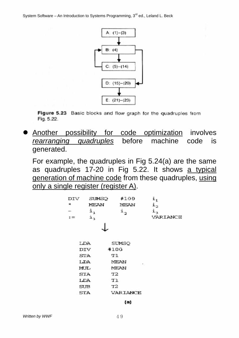
Another possibility for code optimization involves

rearranging quadruples before machine code is generated. For example, the quadruples in Fig 5.24(a) are the same as quadruples 17-20 in Fig 5.22. It shows a typical generation of machine code from these quadruples, using only a single register (register A).

Written by WWF ４９


In Fig 5.24(a), since i2 has just been computed, its value is available in register A; however, this does no good, since the first operand for a ‘–‘ operation must be in the register. It is necessary to store the value of i2 in another temporary variable, T2, and then load the value of i1 from T1 into register A before performing the subtraction.

With a little analysis, an optimizing compiler could recognize this situation and rearrange the quadruples so the 2nd operand of the subtraction is computed first. This rearrangement is illustrated in Fig 5.24(b).

The resulting machine code requires two fewer instructions and uses only one temporary variable instead of two.

Other possibilities for machine-dependent code optimization involve taking advantage of specific characteristics and instructions of target machine. For example, there may be special loop-control instructions or addressing modes that can be used to create more efficient object code.

Written by WWF ５０

Documents

Chapter 5 –Compilers - Maniramanathaenggnotebook.weebly.com/.../chapter_5compilersnew.pdf · Chapter 5 – Compilers ... grammar. This grammar specifies the form, ... z After the