Chapter 4: Probability Distributions

4.1 Random Variables

A random variable is a function X that assigns a numerical value x to each possible outcome in the sample space

An event can be associated with a single value of the random variable, or it can be associated with a range of values of the random variable. The probability of an event can then be described as: 𝑃 𝐴 = 𝑃(𝑋 = 𝑥𝑖) or 𝑃 𝐴 = 𝑃(𝑥𝑙 ≤ 𝑋 ≤ 𝑥𝑢) There could also be other topology for the random variable to describe the event. If 𝑥𝑖 , 𝑖 = 1,2,⋯ ,𝑁 are all the possible values of random variable associated with the sample space, then

𝑃(𝑋 = 𝑥𝑖)

𝑁

𝑖=1

= 1

𝑀1

𝑀2

𝑃1

𝑃2

𝑃1

𝐶1

𝐶2

𝐶3

𝐶1

𝐶2

𝐶3

𝐶1

𝐶2

𝐶3

probabilities 0.03

0.06

0.07

0.02

0.01

0.01

0.09

0.16

0.01 …

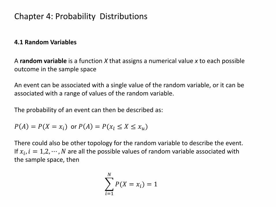
e.g. Each (composite) outcome consists of 3 ratings (M,P,C). Let 𝑀1 , 𝑃1 and 𝐶1 be preferred ratings. Let X be the function that assigns to each outcome the number of preferred ratings each outcome possesses.

Since each outcome has a probability, we can compute the probability of getting each value x = 0,1,2,3 of the function X

x 3

2

2

2

1

1

2

1

1 …

x | P(X = x) 3 | 0.03 2 | 0.29 1 | 0.50 0 | 0.18

Random variables X can be classified by the number of values x they can assume. The two common types are discrete random variables with a finite or countably infinite number of values continuous random variables having a continuum of values for x 1. A value of a random variable may correspond to several random events. 2. An event may correspond to a range of values (or ranges of values) of a

random variable. 3. But a given value (in its legal range) of a random variable corresponds to a

random event. 4. Different random values of the random variable correspond to mutually

exclusive random events. 5. Each value of a random variable has a corresponding probability. 6. All possible values of a random variable correspond to the entire sample

space. 7. The summation of probabilities corresponding to all values of a random

variable must equal to unity.

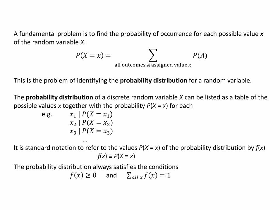
A fundamental problem is to find the probability of occurrence for each possible value x of the random variable X.

𝑃 𝑋 = 𝑥 = 𝑃(𝐴)

all outcomes 𝐴 assigned value 𝑥

This is the problem of identifying the probability distribution for a random variable. The probability distribution of a discrete random variable X can be listed as a table of the possible values x together with the probability P(X = x) for each e.g. 𝑥1 | 𝑃(𝑋 = 𝑥1) 𝑥2 | 𝑃(𝑋 = 𝑥2) 𝑥3 | 𝑃(𝑋 = 𝑥3) … It is standard notation to refer to the values P(X = x) of the probability distribution by f(x) f(x) ≡ P(X = x)

The probability distribution always satisfies the conditions 𝑓 𝑥 ≥ 0 and 𝑓 𝑥 = 1𝑎𝑙𝑙 𝑥

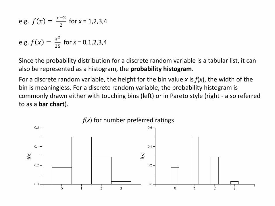
e.g. 𝑓 𝑥 = 𝑥−2

2 for x = 1,2,3,4

e.g. 𝑓 𝑥 = 𝑥2

25 for x = 0,1,2,3,4

Since the probability distribution for a discrete random variable is a tabular list, it can also be represented as a histogram, the probability histogram.

For a discrete random variable, the height for the bin value x is f(x), the width of the bin is meaningless. For a discrete random variable, the probability histogram is commonly drawn either with touching bins (left) or in Pareto style (right - also referred to as a bar chart).

f(x) for number preferred ratings

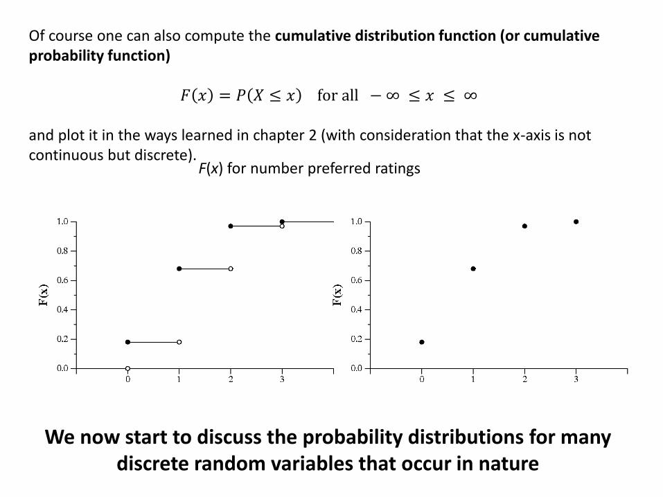
Of course one can also compute the cumulative distribution function (or cumulative probability function)

𝐹 𝑥 = 𝑃 𝑋 ≤ 𝑥 for all − ∞ ≤ 𝑥 ≤ ∞ and plot it in the ways learned in chapter 2 (with consideration that the x-axis is not continuous but discrete).

We now start to discuss the probability distributions for many discrete random variables that occur in nature

F(x) for number preferred ratings

4.2 Binomial Distribution

Bernoulli distribution: In probability theory and statistics, the Bernoulli distribution, named after Swiss scientist Jacob Bernoulli, is a discrete probability distribution, which takes value 1 with success probability 𝑝 and value 0 with failure probability 𝑞 = 1 − 𝑝 . So if X is a random variable with this distribution, we have:

𝑃 𝑋 = 1 = 𝑝; 𝑝 𝑋 = 0 = 𝑞 = 1 − 𝑝. Mean and variance of a random variable 𝑿: (1) Mean (mathematical expectation, expectation, average, etc):

𝜇 = 𝑥 = 𝐸 𝑋 = 𝑥𝑃(𝑋 = 𝑥)

𝑖

(2) Variance:

𝑉𝑎𝑟 𝑋 = 𝐸 𝑥 − 𝑥 2 = 𝜎2 = 𝑥 − 𝜇 2𝑃(𝑋 = 𝑥)𝑖

𝜎 is called the standard deviation. For random variable with Bernoulli distribution, we have

𝜇 = 𝐸 𝑋 = 𝑝 𝑉𝑎𝑟 𝑋 = 𝜎2 = 1 − 𝑝 2𝑝 + 𝑝2𝑞 = 𝑞2𝑝 + 𝑝2𝑞 = 𝑝𝑞 𝑝 + 𝑞 = 𝑝𝑞

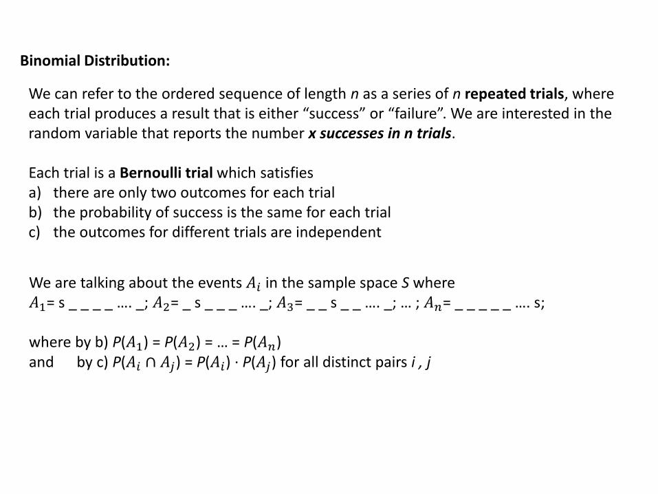
Binomial Distribution: We can refer to the ordered sequence of length n as a series of n repeated trials, where each trial produces a result that is either “success” or “failure”. We are interested in the random variable that reports the number x successes in n trials. Each trial is a Bernoulli trial which satisfies a) there are only two outcomes for each trial b) the probability of success is the same for each trial c) the outcomes for different trials are independent

We are talking about the events 𝐴𝑖 in the sample space S where 𝐴1= s _ _ _ _ …. _; 𝐴2= _ s _ _ _ …. _; 𝐴3= _ _ s _ _ …. _; … ; 𝐴𝑛= _ _ _ _ _ …. s; where by b) P(𝐴1) = P(𝐴2) = … = P(𝐴𝑛) and by c) P(𝐴𝑖 ∩ 𝐴𝑗) = P(𝐴𝑖) · P(𝐴𝑗) for all distinct pairs i , j

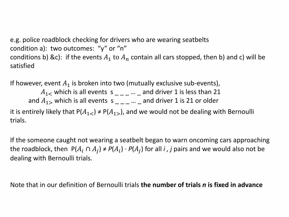
e.g. police roadblock checking for drivers who are wearing seatbelts condition a): two outcomes: “y” or “n” conditions b) &c): if the events 𝐴1 to 𝐴𝑛 contain all cars stopped, then b) and c) will be satisfied If however, event 𝐴1 is broken into two (mutually exclusive sub-events), 𝐴1< which is all events s _ _ _ … _ and driver 1 is less than 21 and 𝐴1> which is all events s _ _ _ … _ and driver 1 is 21 or older

it is entirely likely that P(𝐴1<) ≠ P(𝐴1>), and we would not be dealing with Bernoulli trials.

If the someone caught not wearing a seatbelt began to warn oncoming cars approaching the roadblock, then P(𝐴𝑖 ∩ 𝐴𝑗) ≠ P(𝐴𝑖) · P(𝐴𝑗) for all i , j pairs and we would also not be

dealing with Bernoulli trials.

Note that in our definition of Bernoulli trials the number of trials n is fixed in advance

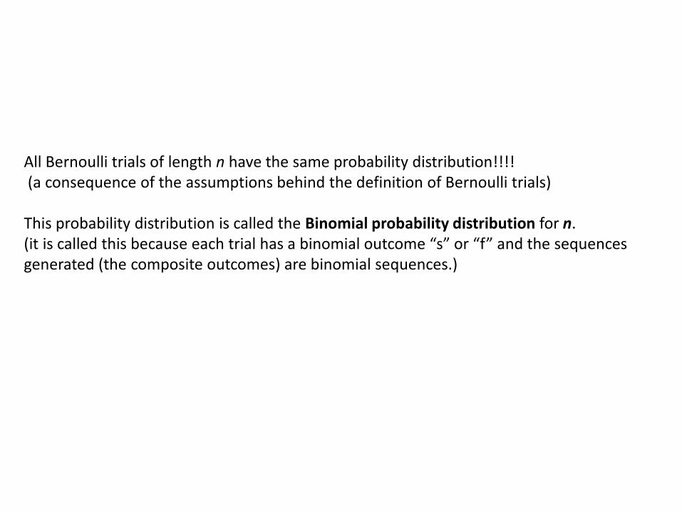
All Bernoulli trials of length n have the same probability distribution!!!! (a consequence of the assumptions behind the definition of Bernoulli trials) This probability distribution is called the Binomial probability distribution for n. (it is called this because each trial has a binomial outcome “s” or “f” and the sequences generated (the composite outcomes) are binomial sequences.)

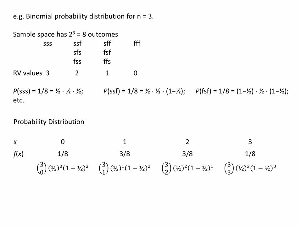
Probability Distribution

x 0 1 2 3

f(x) 1/8 3/8 3/8 1/8

30½ 0 1 −½ 3

31½ 1 1 −½ 2

32½ 2 1 −½ 1

33½ 3 1 −½ 0

e.g. Binomial probability distribution for n = 3. Sample space has 23 = 8 outcomes sss ssf sff fff sfs fsf fss ffs

RV values 3 2 1 0 P(sss) = 1/8 = ½ · ½ · ½; P(ssf) = 1/8 = ½ · ½ · (1−½); P(fsf) = 1/8 = (1−½) · ½ · (1−½); etc.

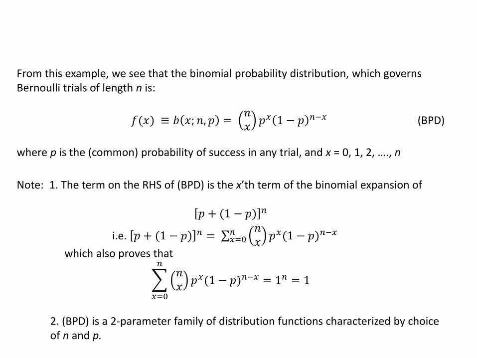
From this example, we see that the binomial probability distribution, which governs Bernoulli trials of length n is:

𝑓(𝑥) ≡ 𝑏 𝑥; 𝑛, 𝑝 = 𝑛𝑥𝑝𝑥 1 − 𝑝 𝑛−𝑥 (BPD)

where p is the (common) probability of success in any trial, and x = 0, 1, 2, …., n

Note: 1. The term on the RHS of (BPD) is the x’th term of the binomial expansion of

𝑝 + (1 − 𝑝) 𝑛

i.e. 𝑝 + (1 − 𝑝) 𝑛 = 𝑛𝑥𝑝𝑥(1 − 𝑝)𝑛−𝑥𝑛

𝑥=0

which also proves that

𝑛𝑥𝑝𝑥(1 − 𝑝)𝑛−𝑥

𝑛

𝑥=0

= 1𝑛 = 1

2. (BPD) is a 2-parameter family of distribution functions characterized by choice of n and p.

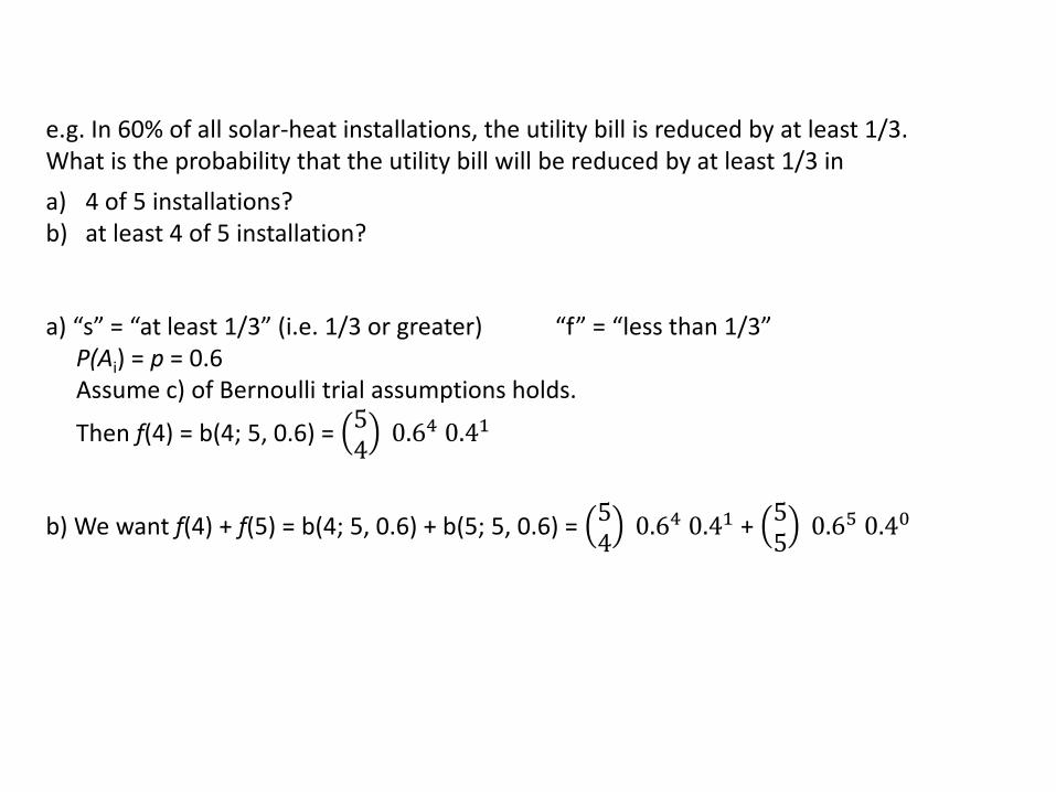
e.g. In 60% of all solar-heat installations, the utility bill is reduced by at least 1/3. What is the probability that the utility bill will be reduced by at least 1/3 in

a) 4 of 5 installations? b) at least 4 of 5 installation?

a) “s” = “at least 1/3” (i.e. 1/3 or greater) “f” = “less than 1/3” P(Ai) = p = 0.6 Assume c) of Bernoulli trial assumptions holds.

Then f(4) = b(4; 5, 0.6) = 54 0.64 0.41

b) We want f(4) + f(5) = b(4; 5, 0.6) + b(5; 5, 0.6) = 54 0.64 0.41 +

55 0.65 0.40

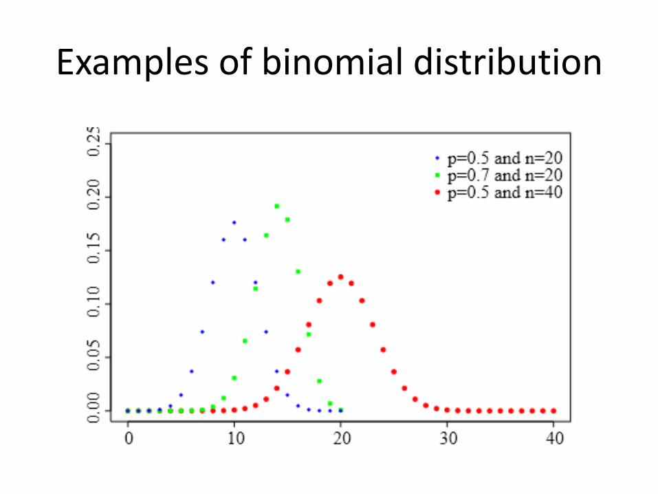
Examples of binomial distribution

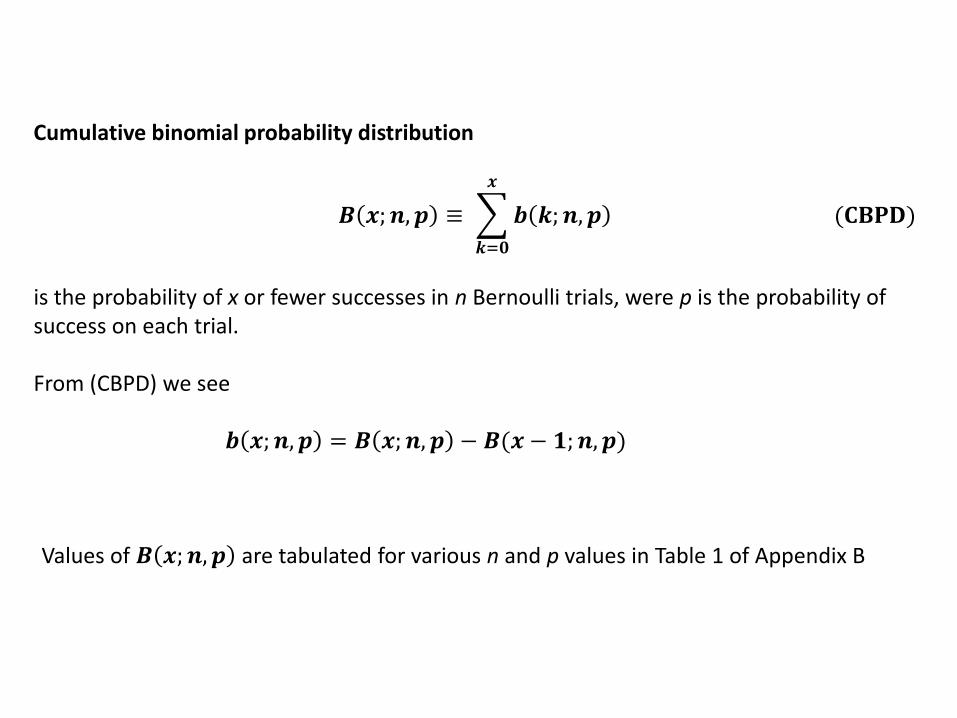
Cumulative binomial probability distribution

𝑩 𝒙;𝒏, 𝒑 ≡ 𝒃 𝒌;𝒏, 𝒑

𝒙

𝒌=𝟎

(𝐂𝐁𝐏𝐃)

is the probability of x or fewer successes in n Bernoulli trials, were p is the probability of success on each trial. From (CBPD) we see 𝒃 𝒙; 𝒏, 𝒑 = 𝑩 𝒙;𝒏, 𝒑 − 𝑩(𝒙 − 𝟏;𝒏, 𝒑)

Values of 𝑩 𝒙;𝒏, 𝒑 are tabulated for various n and p values in Table 1 of Appendix B

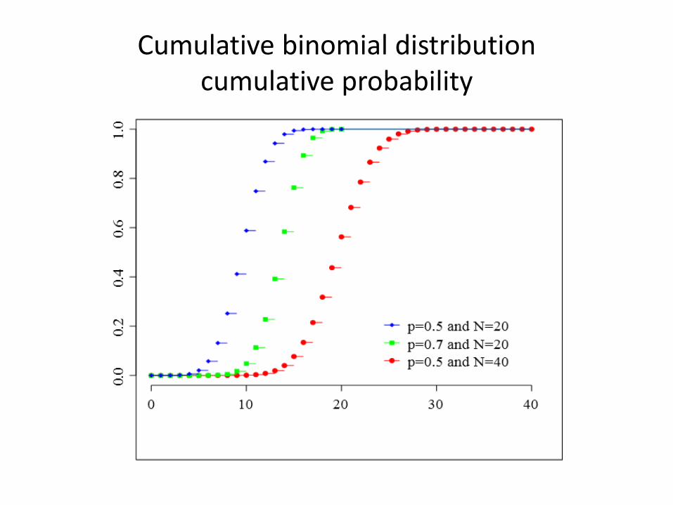
Cumulative binomial distribution cumulative probability

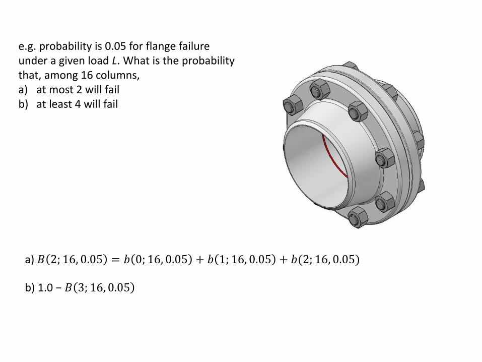
e.g. probability is 0.05 for flange failure under a given load L. What is the probability that, among 16 columns, a) at most 2 will fail b) at least 4 will fail

a) 𝐵 2; 16, 0.05 = 𝑏 0; 16, 0.05 + 𝑏 1; 16, 0.05 + 𝑏(2; 16, 0.05)

b) 1.0 − 𝐵 3; 16, 0.05

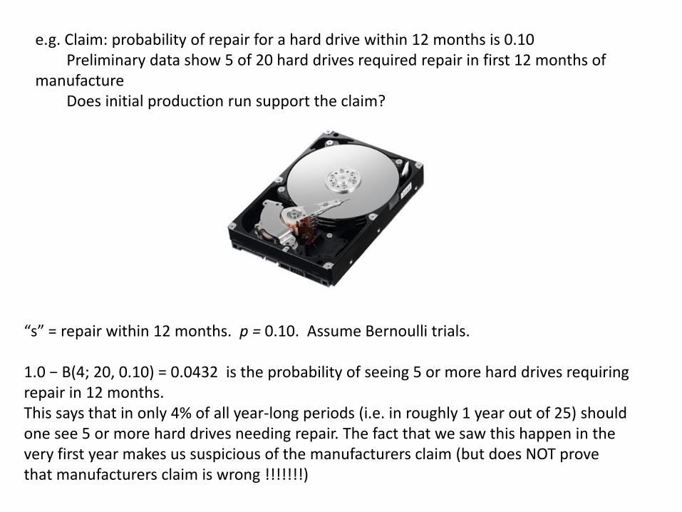
e.g. Claim: probability of repair for a hard drive within 12 months is 0.10 Preliminary data show 5 of 20 hard drives required repair in first 12 months of manufacture Does initial production run support the claim?

“s” = repair within 12 months. p = 0.10. Assume Bernoulli trials. 1.0 − B(4; 20, 0.10) = 0.0432 is the probability of seeing 5 or more hard drives requiring repair in 12 months. This says that in only 4% of all year-long periods (i.e. in roughly 1 year out of 25) should one see 5 or more hard drives needing repair. The fact that we saw this happen in the very first year makes us suspicious of the manufacturers claim (but does NOT prove that manufacturers claim is wrong !!!!!!!)

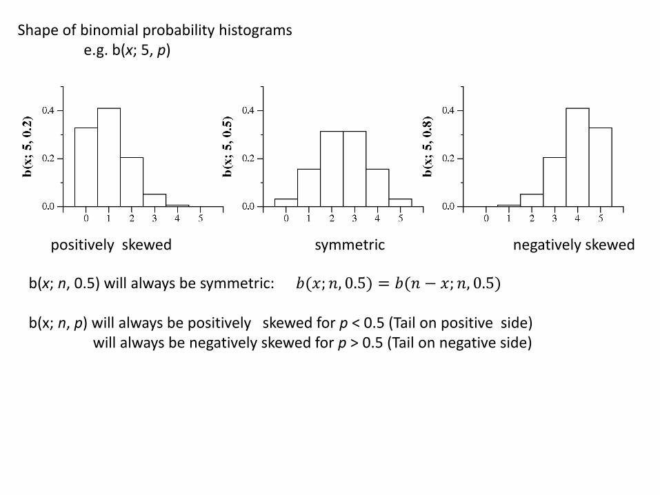
Shape of binomial probability histograms e.g. b(x; 5, p)

positively skewed symmetric negatively skewed

b(x; n, 0.5) will always be symmetric: b(x; n, p) will always be positively skewed for p < 0.5 (Tail on positive side) will always be negatively skewed for p > 0.5 (Tail on negative side)

𝑏(𝑥; 𝑛, 0.5) = 𝑏(𝑛 − 𝑥; 𝑛, 0.5)

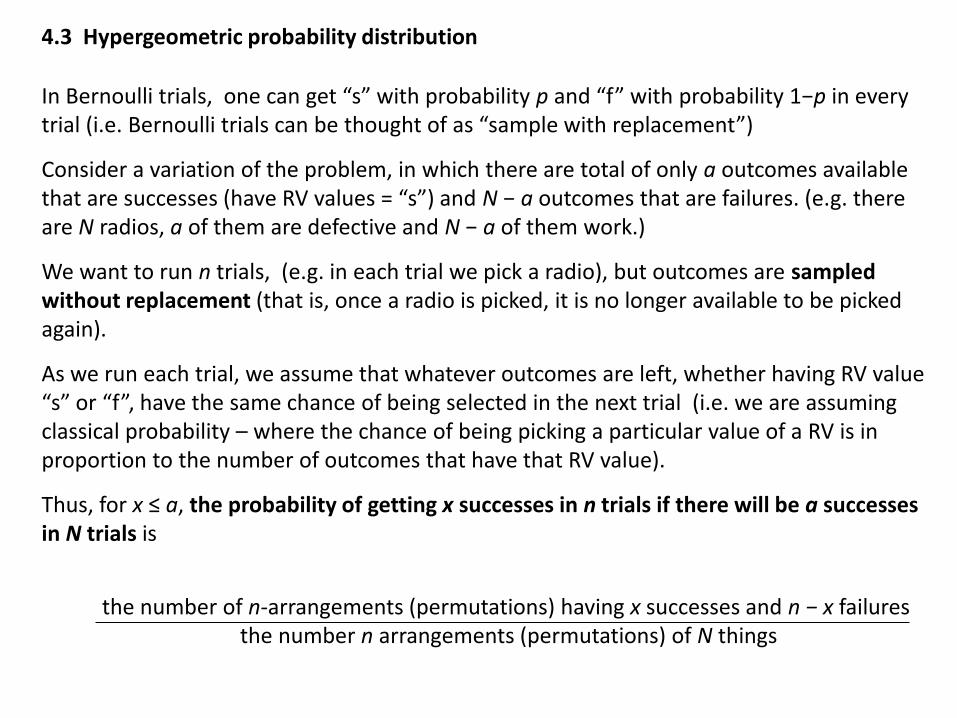
4.3 Hypergeometric probability distribution

In Bernoulli trials, one can get “s” with probability p and “f” with probability 1−p in every trial (i.e. Bernoulli trials can be thought of as “sample with replacement”)

Consider a variation of the problem, in which there are total of only a outcomes available that are successes (have RV values = “s”) and N − a outcomes that are failures. (e.g. there are N radios, a of them are defective and N − a of them work.)

We want to run n trials, (e.g. in each trial we pick a radio), but outcomes are sampled without replacement (that is, once a radio is picked, it is no longer available to be picked again).

As we run each trial, we assume that whatever outcomes are left, whether having RV value “s” or “f”, have the same chance of being selected in the next trial (i.e. we are assuming classical probability – where the chance of being picking a particular value of a RV is in proportion to the number of outcomes that have that RV value).

Thus, for x ≤ a, the probability of getting x successes in n trials if there will be a successes in N trials is

the number of n-arrangements (permutations) having x successes and n − x failures

the number n arrangements (permutations) of N things

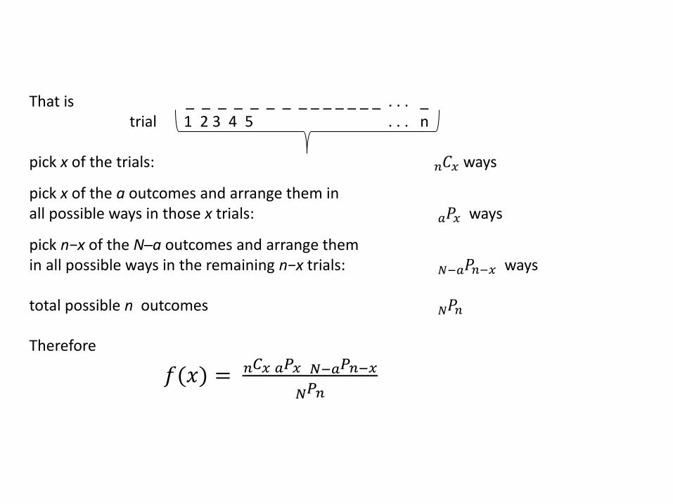
That is _ _ _ _ _ _ _ _ _ _ _ _ _ _ . . . _ trial 1 2 3 4 5 . . . n pick x of the trials: 𝐶𝑥𝑛 ways

pick x of the a outcomes and arrange them in all possible ways in those x trials: 𝑃𝑥𝑎 ways

pick n−x of the N─a outcomes and arrange them in all possible ways in the remaining n−x trials: 𝑃𝑛−𝑥𝑁−𝑎 ways total possible n outcomes 𝑃𝑛𝑁 Therefore

𝑓(𝑥) = 𝐶𝑥 𝑃𝑥 𝑃𝑛−𝑥𝑁−𝑎𝑎𝑛

𝑃𝑛𝑁

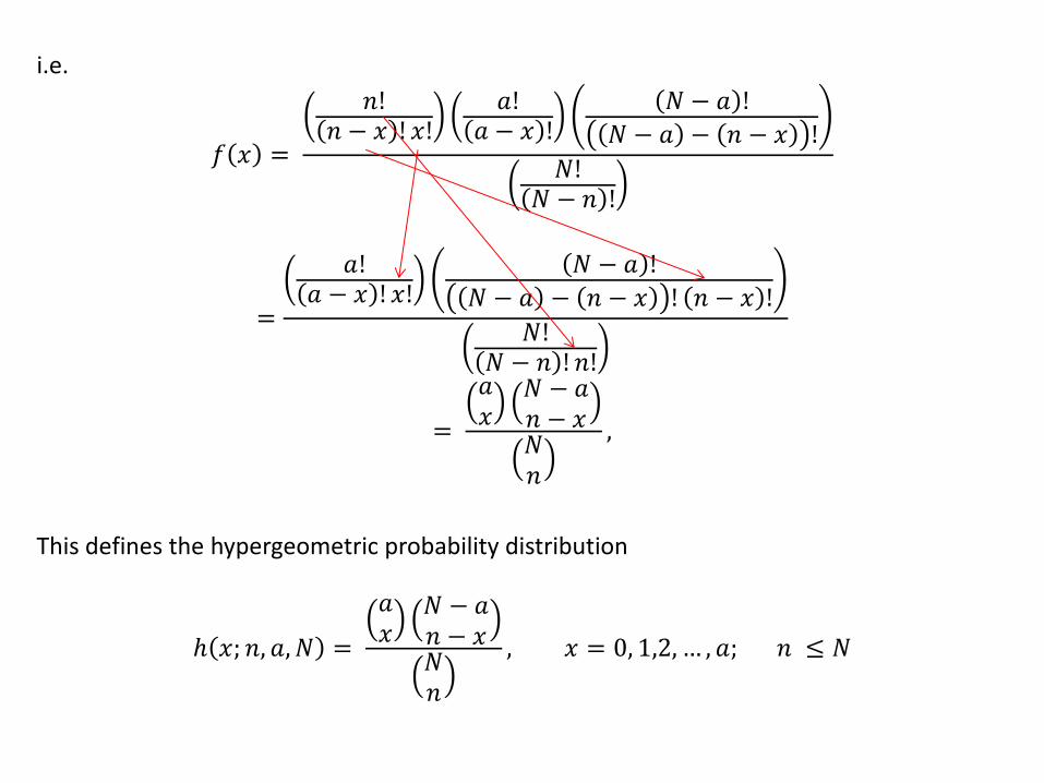
i.e.

𝑓 𝑥 =

𝑛!𝑛 − 𝑥 ! 𝑥!

𝑎!𝑎 − 𝑥 !

𝑁 − 𝑎 !

𝑁 − 𝑎 − 𝑛 − 𝑥 !

𝑁!𝑁 − 𝑛 !

=

𝑎!𝑎 − 𝑥 ! 𝑥!

𝑁 − 𝑎 !

𝑁 − 𝑎 − 𝑛 − 𝑥 ! 𝑛 − 𝑥 !

𝑁!𝑁 − 𝑛 ! 𝑛!

=

𝑎𝑥𝑁 − 𝑎𝑛 − 𝑥𝑁𝑛

,

This defines the hypergeometric probability distribution

ℎ 𝑥; 𝑛, 𝑎, 𝑁 =

𝑎𝑥𝑁 − 𝑎𝑛 − 𝑥𝑁𝑛

, 𝑥 = 0, 1,2, … , 𝑎; 𝑛 ≤ 𝑁

e.g. PC has 20 identical car chargers, 5 are defective. PC will randomly ship 10. What is the probability that 2 of those shipped will be defective?

ℎ 2; 10,5,20 =

521582010

=

5!3! 2!

15!7! 8!20!10! 10!

= 5! 15! 10! 10!

3! 2! 7! 8! 20!= 5!

3! 2!

15!

20!

10!

7!

10!

8!

= 5 4

2

1

20 19 18 17 16

10 9 8 10 9=5 4

2

10

20

9

18

8

16

10

19

9

17=5 4

2

1

2

1

2

1

2

10

19

9

17

= 5

2 5

19 9

17= 0.348

e.g. redo using 100 car chargers and 25 defective

ℎ 2; 10,25,100 =

252758

10010

= 0.292

e.g. approximate this using the binomial distribution

b 2; 10, 𝑝 ≈ 25/100 =102 0.252 0.758= 0.282

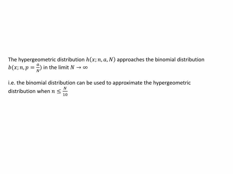
The hypergeometric distribution ℎ 𝑥; 𝑛, 𝑎, 𝑁 approaches the binomial distribution

𝑏(𝑥; 𝑛, 𝑝 =𝑎

𝑁) in the limit 𝑁 → ∞

i.e. the binomial distribution can be used to approximate the hypergeometric

distribution when 𝑛 ≤𝑁

10

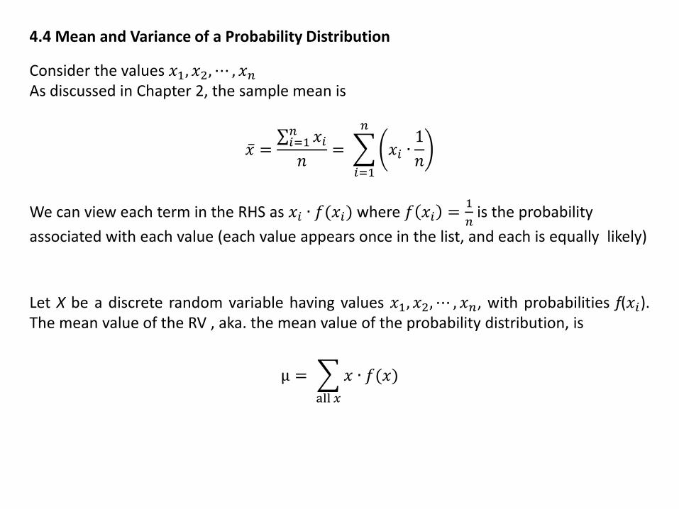
4.4 Mean and Variance of a Probability Distribution

Consider the values 𝑥1, 𝑥2, ⋯ , 𝑥𝑛 As discussed in Chapter 2, the sample mean is

𝑥 = 𝑥𝑖𝑛𝑖=1

𝑛= 𝑥𝑖 ∙

1

𝑛

𝑛

𝑖=1

We can view each term in the RHS as 𝑥𝑖 ∙ 𝑓(𝑥𝑖) where 𝑓 𝑥𝑖 =1

𝑛 is the probability

associated with each value (each value appears once in the list, and each is equally likely)

Let X be a discrete random variable having values 𝑥1, 𝑥2, ⋯ , 𝑥𝑛, with probabilities f(𝑥𝑖). The mean value of the RV , aka. the mean value of the probability distribution, is

μ = 𝑥 ∙ 𝑓(𝑥)

all 𝑥

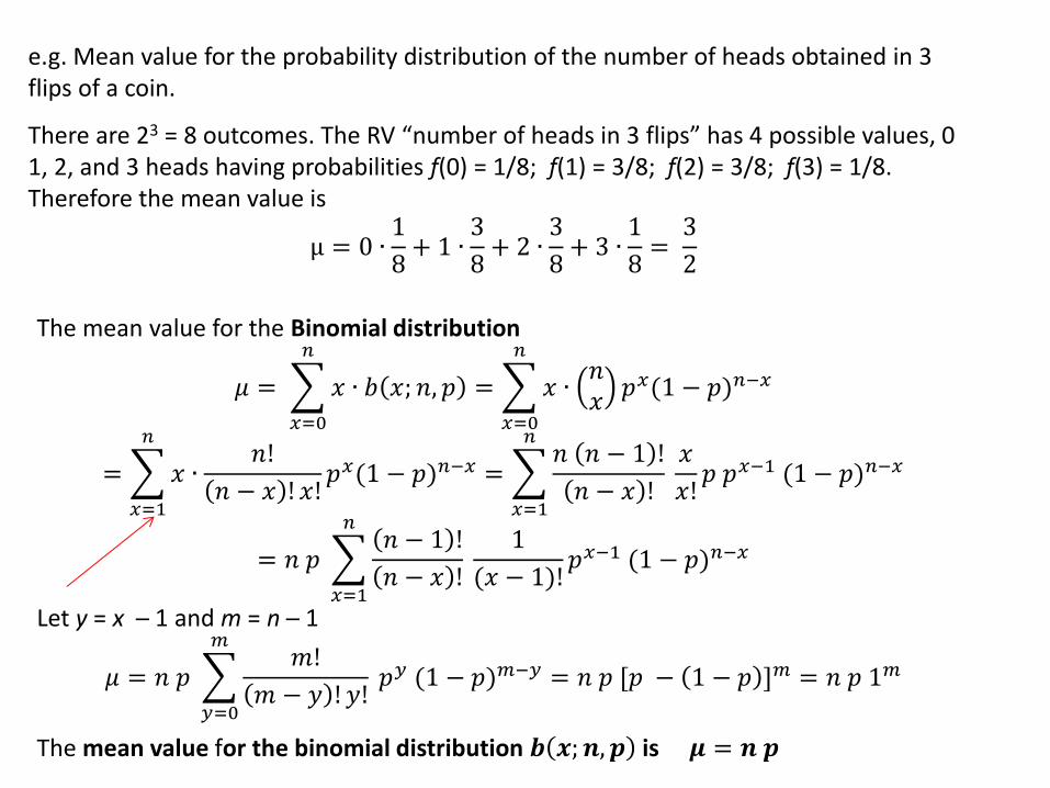
e.g. Mean value for the probability distribution of the number of heads obtained in 3 flips of a coin.

There are 23 = 8 outcomes. The RV “number of heads in 3 flips” has 4 possible values, 0 1, 2, and 3 heads having probabilities f(0) = 1/8; f(1) = 3/8; f(2) = 3/8; f(3) = 1/8. Therefore the mean value is

μ = 0 ∙1

8+ 1 ∙3

8+ 2 ∙3

8+ 3 ∙1

8= 3

2

The mean value for the Binomial distribution

𝜇 = 𝑥 ∙ 𝑏 𝑥; 𝑛, 𝑝 = 𝑥 ∙𝑛𝑥𝑝𝑥(1 − 𝑝)𝑛−𝑥

𝑛

𝑥=0

𝑛

𝑥=0

= 𝑥 ∙𝑛!

𝑛 − 𝑥 ! 𝑥!𝑝𝑥(1 − 𝑝)𝑛−𝑥

𝑛

𝑥=1

= 𝑛 𝑛 − 1 !

𝑛 − 𝑥 ! 𝑥

𝑥!𝑝 𝑝𝑥−1 (1 − 𝑝)𝑛−𝑥

𝑛

𝑥=1

= 𝑛 𝑝 𝑛 − 1 !

𝑛 − 𝑥 ! 1

(𝑥 − 1)!𝑝𝑥−1 (1 − 𝑝)𝑛−𝑥

𝑛

𝑥=1

Let y = x ─ 1 and m = n ─ 1

𝜇 = 𝑛 𝑝 𝑚!

𝑚 − 𝑦 ! 𝑦! 𝑝𝑦 (1 − 𝑝)𝑚−𝑦

𝑚

𝑦=0

= 𝑛 𝑝 [𝑝 − 1 − 𝑝 ]𝑚 = 𝑛 𝑝 1𝑚

The mean value for the binomial distribution 𝒃 𝒙; 𝒏, 𝒑 is 𝝁 = 𝒏 𝒑

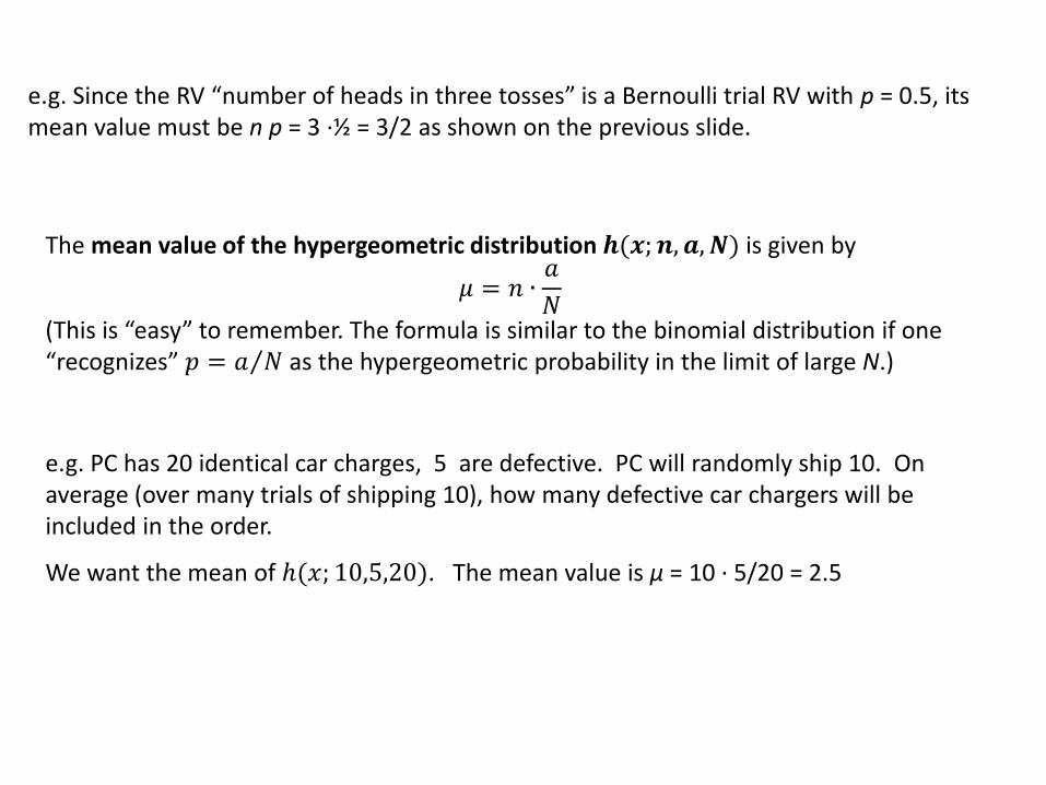
e.g. Since the RV “number of heads in three tosses” is a Bernoulli trial RV with p = 0.5, its mean value must be n p = 3 ·½ = 3/2 as shown on the previous slide.

The mean value of the hypergeometric distribution 𝒉(𝒙; 𝒏, 𝒂, 𝑵) is given by

𝜇 = 𝑛 ∙𝑎

𝑁

(This is “easy” to remember. The formula is similar to the binomial distribution if one “recognizes” 𝑝 = 𝑎 𝑁 as the hypergeometric probability in the limit of large N.)

e.g. PC has 20 identical car charges, 5 are defective. PC will randomly ship 10. On average (over many trials of shipping 10), how many defective car chargers will be included in the order.

We want the mean of ℎ(𝑥; 10,5,20). The mean value is μ = 10 · 5/20 = 2.5

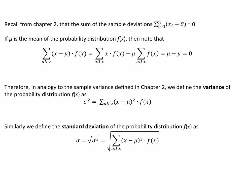
Recall from chapter 2, that the sum of the sample deviations 𝑥𝑖 − 𝑥 𝑛𝑖=1 = 0

If μ is the mean of the probability distribution f(x), then note that

𝑥 − 𝜇 ∙ 𝑓(𝑥)

𝑎𝑙𝑙 𝑥

= 𝑥 ∙ 𝑓 𝑥 − 𝜇 𝑓 𝑥

𝑎𝑙𝑙 𝑥𝑎𝑙𝑙 𝑥

= 𝜇 − 𝜇 = 0

Therefore, in analogy to the sample variance defined in Chapter 2, we define the variance of the probability distribution f(x) as

𝜎2 = 𝑥 − 𝜇 2 ∙ 𝑓(𝑥)𝑎𝑙𝑙 𝑥

Similarly we define the standard deviation of the probability distribution f(x) as

𝜎 = 𝜎2 = 𝑥 − 𝜇 2 ∙ 𝑓(𝑥)

𝑎𝑙𝑙 𝑥

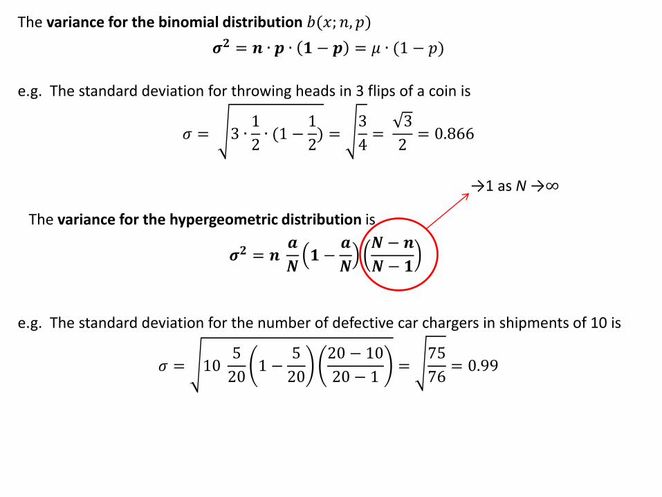
The variance for the binomial distribution 𝑏(𝑥; 𝑛, 𝑝)

𝝈𝟐 = 𝒏 ∙ 𝒑 ∙ 𝟏 − 𝒑 = 𝜇 ∙ (1 − 𝑝)

e.g. The standard deviation for throwing heads in 3 flips of a coin is

𝜎 = 3 ∙1

2∙ (1 −1

2) =3

4= 3

2= 0.866

The variance for the hypergeometric distribution is

𝝈𝟐 = 𝒏 𝒂

𝑵𝟏 −𝒂

𝑵

𝑵− 𝒏

𝑵− 𝟏

e.g. The standard deviation for the number of defective car chargers in shipments of 10 is

𝜎 = 10 5

201 −5

20

20 − 10

20 − 1=75

76= 0.99

→1 as N →∞

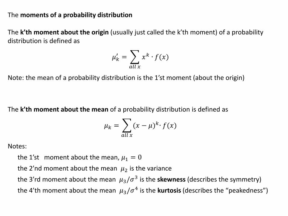
The moments of a probability distribution The k’th moment about the origin (usually just called the k’th moment) of a probability distribution is defined as

𝜇𝑘′ = 𝑥𝑘 ∙ 𝑓(𝑥)

𝑎𝑙𝑙 𝑥

Note: the mean of a probability distribution is the 1’st moment (about the origin)

The k’th moment about the mean of a probability distribution is defined as

𝜇𝑘 = (𝑥 − 𝜇)𝑘∙ 𝑓(𝑥)

𝑎𝑙𝑙 𝑥

Notes:

the 1’st moment about the mean, 𝜇1 = 0

the 2’nd moment about the mean 𝜇2 is the variance

the 3’rd moment about the mean 𝜇3/𝜎3 is the skewness (describes the symmetry)

the 4’th moment about the mean 𝜇3/𝜎4 is the kurtosis (describes the “peakedness”)

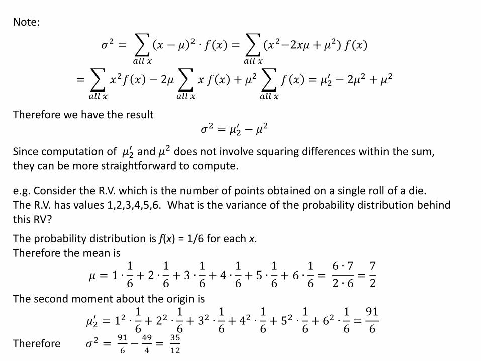
Note:

𝜎2 = 𝑥 − 𝜇 2 ∙ 𝑓(𝑥)

𝑎𝑙𝑙 𝑥

= (𝑥2−2𝑥𝜇 + 𝜇2) 𝑓(𝑥)

𝑎𝑙𝑙 𝑥

= 𝑥2𝑓 𝑥 − 2𝜇 𝑥 𝑓 𝑥

𝑎𝑙𝑙 𝑥

+ 𝜇2 𝑓 𝑥

𝑎𝑙𝑙 𝑥

= 𝜇2′ − 2𝜇2 + 𝜇2

𝑎𝑙𝑙 𝑥

Therefore we have the result 𝜎2 = 𝜇2

′ − 𝜇2

Since computation of 𝜇2′ and 𝜇2 does not involve squaring differences within the sum,

they can be more straightforward to compute.

e.g. Consider the R.V. which is the number of points obtained on a single roll of a die. The R.V. has values 1,2,3,4,5,6. What is the variance of the probability distribution behind this RV?

The probability distribution is f(x) = 1/6 for each x. Therefore the mean is

𝜇 = 1 ∙1

6+ 2 ∙1

6+ 3 ∙1

6+ 4 ∙1

6+ 5 ∙1

6+ 6 ∙1

6= 6 ∙ 7

2 ∙ 6=7

2

The second moment about the origin is

𝜇2′ = 12 ∙

1

6+ 22 ∙

1

6+ 32 ∙

1

6+ 42 ∙

1

6+ 52 ∙

1

6+ 62 ∙

1

6=91

6

Therefore 𝜎2 = 91

6−49

4= 35

12

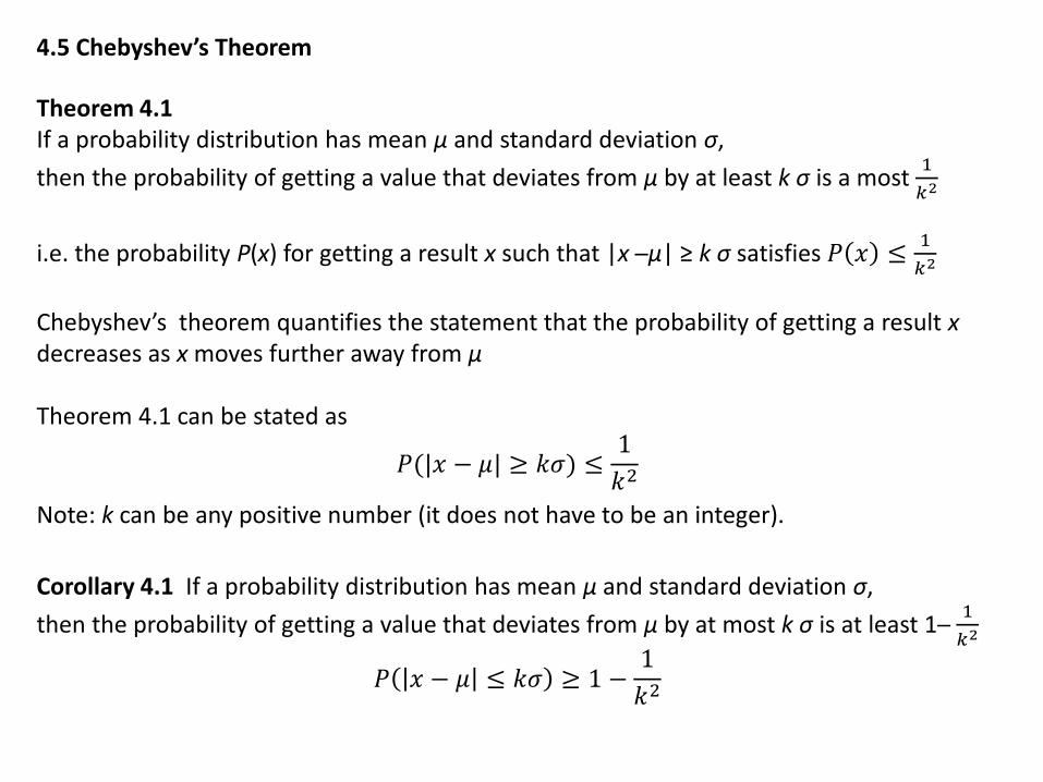
4.5 Chebyshev’s Theorem

Theorem 4.1 If a probability distribution has mean μ and standard deviation σ,

then the probability of getting a value that deviates from μ by at least k σ is a most 1

𝑘2

i.e. the probability P(x) for getting a result x such that |x ─μ| ≥ k σ satisfies 𝑃 𝑥 ≤1

𝑘2

Chebyshev’s theorem quantifies the statement that the probability of getting a result x decreases as x moves further away from μ Theorem 4.1 can be stated as

𝑃(|𝑥 − 𝜇| ≥ 𝑘𝜎) ≤1

𝑘2

Note: k can be any positive number (it does not have to be an integer).

Corollary 4.1 If a probability distribution has mean μ and standard deviation σ,

then the probability of getting a value that deviates from μ by at most k σ is at least 1─ 1

𝑘2

𝑃 𝑥 − 𝜇 ≤ 𝑘𝜎 ≥ 1 −1

𝑘2

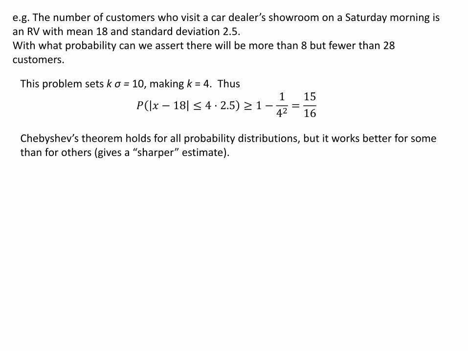
e.g. The number of customers who visit a car dealer’s showroom on a Saturday morning is an RV with mean 18 and standard deviation 2.5. With what probability can we assert there will be more than 8 but fewer than 28 customers.

This problem sets k σ = 10, making k = 4. Thus

𝑃 𝑥 − 18 ≤ 4 · 2.5 ≥ 1 −1

42=15

16

Chebyshev’s theorem holds for all probability distributions, but it works better for some than for others (gives a “sharper” estimate).

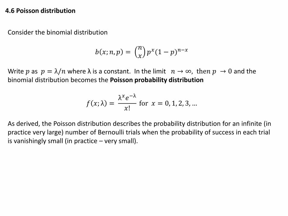
4.6 Poisson distribution

Consider the binomial distribution

𝑏 𝑥; 𝑛, 𝑝 = 𝑛𝑥𝑝𝑥(1 − 𝑝)𝑛−𝑥

Write 𝑝 as 𝑝 = λ/𝑛 where λ is a constant. In the limit 𝑛 → ∞, the𝑛 𝑝 → 0 and the binomial distribution becomes the Poisson probability distribution

𝑓 𝑥; λ = λ𝑥𝑒−λ

𝑥! for 𝑥 = 0, 1, 2, 3, …

As derived, the Poisson distribution describes the probability distribution for an infinite (in practice very large) number of Bernoulli trials when the probability of success in each trial is vanishingly small (in practice – very small).

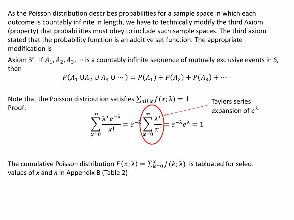
As the Poisson distribution describes probabilities for a sample space in which each outcome is countably infinite in length, we have to technically modify the third Axiom (property) that probabilities must obey to include such sample spaces. The third axiom stated that the probability function is an additive set function. The appropriate modification is

Axiom 3’ If 𝐴1, 𝐴2, 𝐴3, ⋯ is a countably infinite sequence of mutually exclusive events in S, then

𝑃 𝐴1 U𝐴2 ∪ 𝐴3 ∪⋯ = 𝑃 𝐴1 + 𝑃 𝐴2 + 𝑃 𝐴3 +⋯

Note that the Poisson distribution satisfies 𝑓(𝑥; λ)𝑎𝑙𝑙 𝑥 = 1 Proof:

λ𝑥𝑒−λ

𝑥!

∞

𝑥=0

= 𝑒−λ λ𝑥

𝑥!= 𝑒−λ𝑒λ

∞

𝑥=0

= 1

Taylors series

expansion of 𝑒λ

The cumulative Poisson distribution 𝐹 𝑥; λ = 𝑓(𝑘; λ) 𝑥𝑘=0 is tabluated for select

values of x and λ in Appendix B (Table 2)

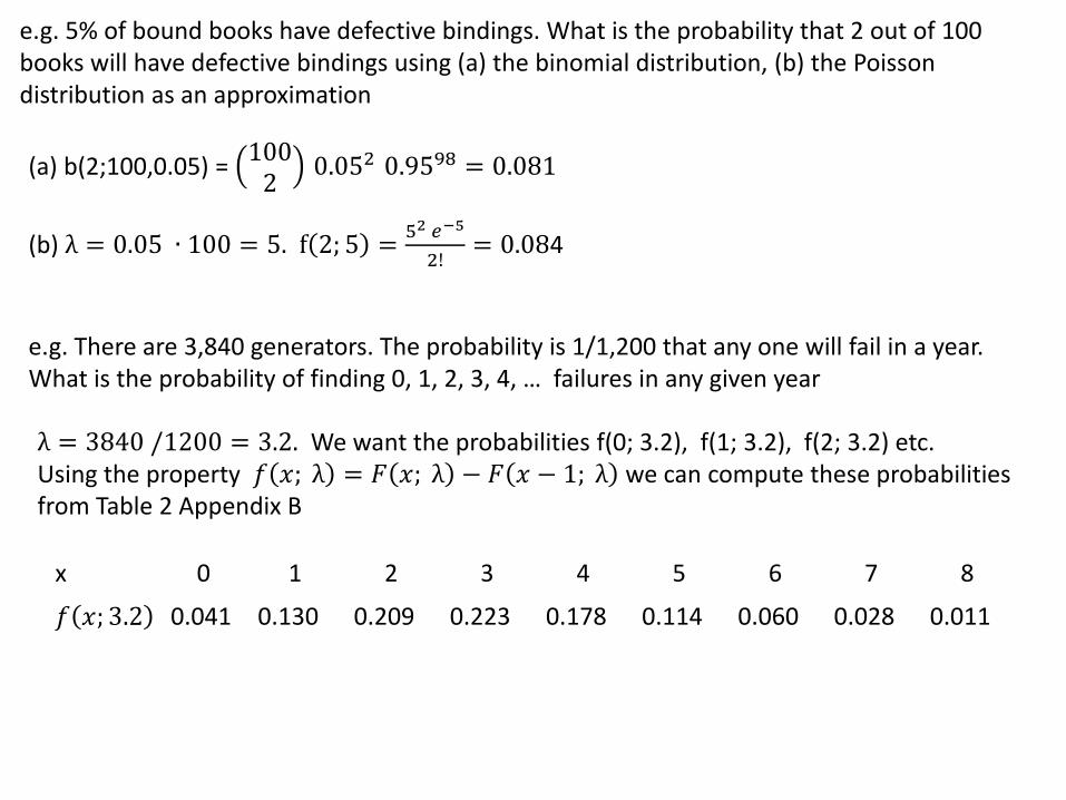
e.g. 5% of bound books have defective bindings. What is the probability that 2 out of 100 books will have defective bindings using (a) the binomial distribution, (b) the Poisson distribution as an approximation

(a) b(2;100,0.05) = 1002 0.052 0.9598 = 0.081

(b) λ = 0.05 ∙ 100 = 5. f 2; 5 =52 𝑒−5

2!= 0.084

e.g. There are 3,840 generators. The probability is 1/1,200 that any one will fail in a year. What is the probability of finding 0, 1, 2, 3, 4, … failures in any given year

λ = 3840 /1200 = 3.2. We want the probabilities f(0; 3.2), f(1; 3.2), f(2; 3.2) etc. Using the property 𝑓 𝑥; λ = 𝐹 𝑥; λ − 𝐹 𝑥 − 1; λ we can compute these probabilities from Table 2 Appendix B

x 0 1 2 3 4 5 6 7 8

𝑓 𝑥; 3.2 0.041 0.130 0.209 0.223 0.178 0.114 0.060 0.028 0.011

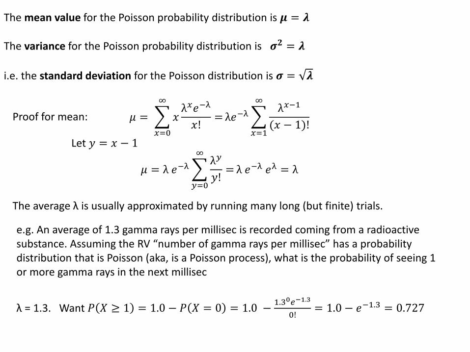
The mean value for the Poisson probability distribution is 𝝁 = 𝝀 The variance for the Poisson probability distribution is 𝝈𝟐 = 𝝀

i.e. the standard deviation for the Poisson distribution is 𝝈 = 𝝀

Proof for mean: 𝜇 = 𝑥λ𝑥𝑒−λ

𝑥!=

∞

𝑥=0

λ𝑒−λ λ𝑥−1

(𝑥 − 1)!

∞

𝑥=1

Let 𝑦 = 𝑥 − 1

𝜇 = λ 𝑒−λ λ𝑦

𝑦!=

∞

𝑦=0

λ 𝑒−λ 𝑒λ = λ

The average λ is usually approximated by running many long (but finite) trials.

e.g. An average of 1.3 gamma rays per millisec is recorded coming from a radioactive substance. Assuming the RV “number of gamma rays per millisec” has a probability distribution that is Poisson (aka, is a Poisson process), what is the probability of seeing 1 or more gamma rays in the next millisec

λ = 1.3. Want 𝑃 𝑋 ≥ 1 = 1.0 − 𝑃 𝑋 = 0 = 1.0 −1.30𝑒−1.3

0!= 1.0 − 𝑒−1.3 = 0.727

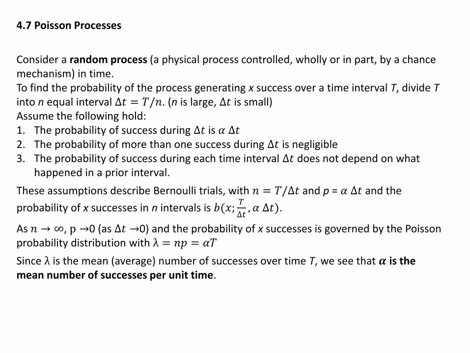
4.7 Poisson Processes

Consider a random process (a physical process controlled, wholly or in part, by a chance mechanism) in time. To find the probability of the process generating x success over a time interval T, divide T into n equal interval ∆𝑡 = 𝑇/𝑛. (n is large, ∆𝑡 is small) Assume the following hold: 1. The probability of success during ∆𝑡 is 𝛼 ∆𝑡 2. The probability of more than one success during ∆𝑡 is negligible 3. The probability of success during each time interval ∆𝑡 does not depend on what

happened in a prior interval.

These assumptions describe Bernoulli trials, with 𝑛 = 𝑇/∆𝑡 and p = 𝛼 ∆𝑡 and the

probability of x successes in n intervals is 𝑏(𝑥;𝑇

∆𝑡, 𝛼 ∆𝑡).

As 𝑛 → ∞, p →0 (as ∆𝑡 →0) and the probability of x successes is governed by the Poisson probability distribution with λ = 𝑛𝑝 = 𝛼𝑇

Since λ is the mean (average) number of successes over time T, we see that 𝜶 is the mean number of successes per unit time.

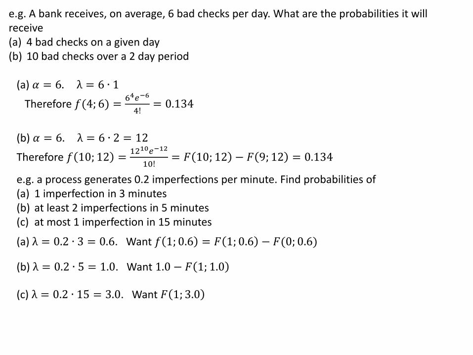
e.g. A bank receives, on average, 6 bad checks per day. What are the probabilities it will receive (a) 4 bad checks on a given day (b) 10 bad checks over a 2 day period

(a) 𝛼 = 6. λ = 6 ∙ 1

Therefore 𝑓(4; 6) =64𝑒−6

4!= 0.134

(b) 𝛼 = 6. λ = 6 ∙ 2 = 12

Therefore 𝑓 10; 12 =1210𝑒−12

10!= 𝐹 10; 12 − 𝐹 9; 12 = 0.134

e.g. a process generates 0.2 imperfections per minute. Find probabilities of (a) 1 imperfection in 3 minutes (b) at least 2 imperfections in 5 minutes (c) at most 1 imperfection in 15 minutes

(a) λ = 0.2 ∙ 3 = 0.6. Want 𝑓 1; 0.6 = 𝐹 1; 0.6 − 𝐹(0; 0.6)

(b) λ = 0.2 ∙ 5 = 1.0. Want 1.0 − 𝐹 1; 1.0

(c) λ = 0.2 ∙ 15 = 3.0. Want 𝐹 1; 3.0

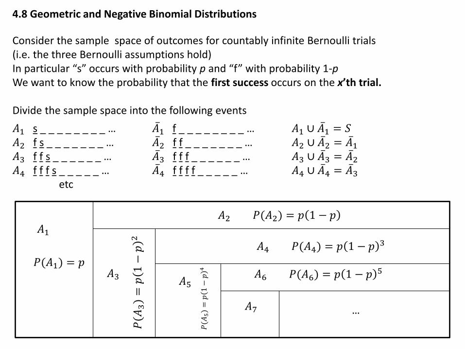
4.8 Geometric and Negative Binomial Distributions

Consider the sample space of outcomes for countably infinite Bernoulli trials (i.e. the three Bernoulli assumptions hold) In particular “s” occurs with probability p and “f” with probability 1-p We want to know the probability that the first success occurs on the x’th trial.

Divide the sample space into the following events

𝐴1 s _ _ _ _ _ _ _ _ … 𝐴 1 f _ _ _ _ _ _ _ _ … 𝐴1 ∪ 𝐴 1 = 𝑆 𝐴2 f s _ _ _ _ _ _ _ … 𝐴 2 f f _ _ _ _ _ _ _ … 𝐴2 ∪ 𝐴 2 = 𝐴 1 𝐴3 f f s _ _ _ _ _ _ … 𝐴 3 f f f _ _ _ _ _ _ … 𝐴3 ∪ 𝐴 3 = 𝐴 2 𝐴4 f f f s _ _ _ _ _ … 𝐴 4 f f f f _ _ _ _ _ … 𝐴4 ∪ 𝐴 4 = 𝐴 3 etc

𝐴1 𝐴2

𝐴3

𝐴4

𝑃(𝐴1) = 𝑝

𝑃(𝐴2) = 𝑝 1 − 𝑝

𝑃(𝐴3)=𝑝1−𝑝2

𝑃(𝐴4) = 𝑝 1 − 𝑝3

𝐴5 𝐴6 𝑃(𝐴6) = 𝑝 1 − 𝑝

5

𝑃(𝐴5)=𝑝1−𝑝4

𝐴7 …

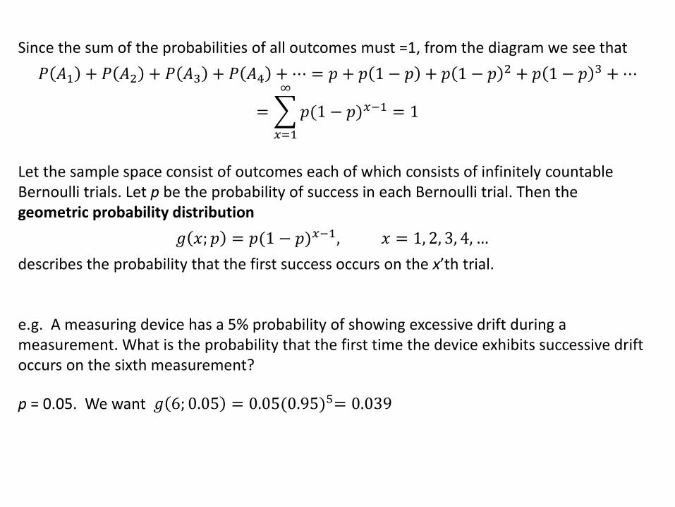
Since the sum of the probabilities of all outcomes must =1, from the diagram we see that

𝑃 𝐴1 + 𝑃 𝐴2 + 𝑃 𝐴3 + 𝑃 𝐴4 +⋯ = 𝑝 + 𝑝 1 − 𝑝 + 𝑝 1 − 𝑝2 + 𝑝 1 − 𝑝 3 +⋯

= 𝑝(1 − 𝑝)𝑥−1∞

𝑥=1

= 1

Let the sample space consist of outcomes each of which consists of infinitely countable Bernoulli trials. Let p be the probability of success in each Bernoulli trial. Then the geometric probability distribution

𝑔 𝑥; 𝑝 = 𝑝(1 − 𝑝)𝑥−1, 𝑥 = 1, 2, 3, 4, …

describes the probability that the first success occurs on the x’th trial.

e.g. A measuring device has a 5% probability of showing excessive drift during a measurement. What is the probability that the first time the device exhibits successive drift occurs on the sixth measurement?

p = 0.05. We want 𝑔 6; 0.05 = 0.05(0.95)5= 0.039

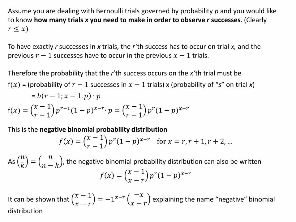
Assume you are dealing with Bernoulli trials governed by probability p and you would like to know how many trials x you need to make in order to observe r successes. (Clearly 𝑟 ≤ 𝑥) To have exactly r successes in x trials, the r’th success has to occur on trial x, and the previous 𝑟 − 1 successes have to occur in the previous 𝑥 − 1 trials. Therefore the probability that the r’th success occurs on the x’th trial must be

f(𝑥) = (probability of 𝑟 − 1 successes in 𝑥 − 1 trials) x (probability of “s” on trial x)

= 𝑏 𝑟 − 1; 𝑥 − 1, 𝑝 ∙ 𝑝

f(𝑥) =𝑥 − 1𝑟 − 1

𝑝𝑟−1(1 − 𝑝)𝑥−𝑟∙ 𝑝 =𝑥 − 1𝑟 − 1

𝑝𝑟(1 − 𝑝)𝑥−𝑟

This is the negative binomial probability distribution

𝑓 𝑥 =𝑥 − 1𝑟 − 1

𝑝𝑟 1 − 𝑝 𝑥−𝑟 for 𝑥 = 𝑟, 𝑟 + 1, 𝑟 + 2,…

As 𝑛𝑘=𝑛𝑛 − 𝑘

, the negative binomial probability distribution can also be written

𝑓 𝑥 =𝑥 − 1𝑥 − 𝑟

𝑝𝑟 1 − 𝑝 𝑥−𝑟

It can be shown that 𝑥 − 1𝑥 − 𝑟

= −1𝑥−𝑟−𝑥𝑥 − 𝑟

explaining the name “negative” binomial

distribution

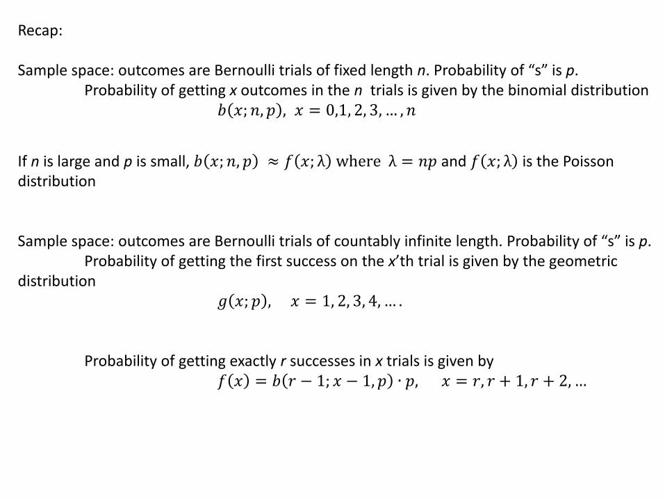
Recap: Sample space: outcomes are Bernoulli trials of fixed length n. Probability of “s” is p. Probability of getting x outcomes in the n trials is given by the binomial distribution 𝑏 𝑥; 𝑛, 𝑝 , 𝑥 = 0,1, 2, 3, … , 𝑛

If n is large and p is small, 𝑏 𝑥; 𝑛, 𝑝 ≈ 𝑓 𝑥; λ where λ = 𝑛𝑝 and 𝑓 𝑥; λ is the Poisson distribution Sample space: outcomes are Bernoulli trials of countably infinite length. Probability of “s” is p. Probability of getting the first success on the x’th trial is given by the geometric distribution 𝑔 𝑥; 𝑝 , 𝑥 = 1, 2, 3, 4, … . Probability of getting exactly r successes in x trials is given by 𝑓 𝑥 = 𝑏 𝑟 − 1; 𝑥 − 1, 𝑝 ∙ 𝑝, 𝑥 = 𝑟, 𝑟 + 1, 𝑟 + 2,…

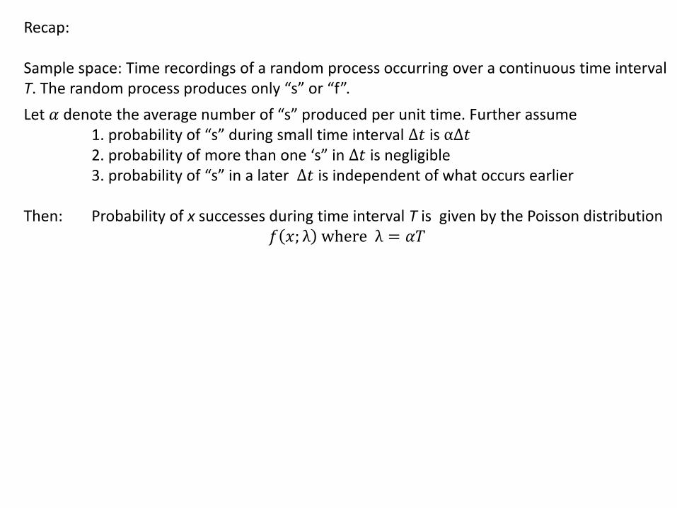
Recap: Sample space: Time recordings of a random process occurring over a continuous time interval T. The random process produces only “s” or “f”.

Let 𝛼 denote the average number of “s” produced per unit time. Further assume 1. probability of “s” during small time interval ∆𝑡 is α∆𝑡 2. probability of more than one ‘s” in ∆𝑡 is negligible 3. probability of “s” in a later ∆𝑡 is independent of what occurs earlier Then: Probability of x successes during time interval T is given by the Poisson distribution

𝑓 𝑥; λ where λ = 𝛼𝑇

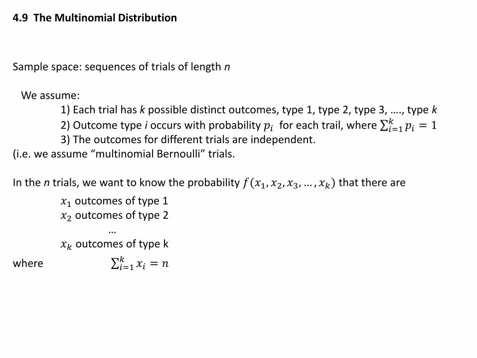
4.9 The Multinomial Distribution

Sample space: sequences of trials of length n We assume: 1) Each trial has k possible distinct outcomes, type 1, type 2, type 3, …., type k

2) Outcome type i occurs with probability 𝑝𝑖 for each trail, where 𝑝𝑖 = 1𝑘𝑖=1

3) The outcomes for different trials are independent. (i.e. we assume “multinomial Bernoulli” trials. In the n trials, we want to know the probability 𝑓(𝑥1, 𝑥2, 𝑥3, … , 𝑥𝑘) that there are

𝑥1 outcomes of type 1 𝑥2 outcomes of type 2 … 𝑥𝑘 outcomes of type k

where 𝑥𝑖 = 𝑛𝑘𝑖=1

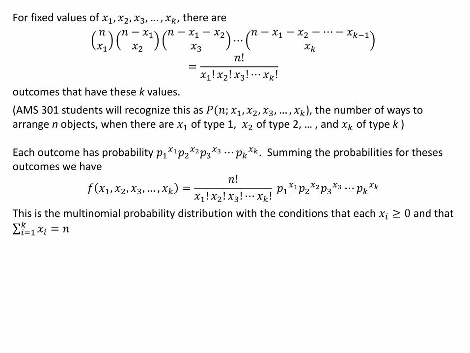
For fixed values of 𝑥1, 𝑥2, 𝑥3, … , 𝑥𝑘, there are 𝑛𝑥1

𝑛 − 𝑥1𝑥2

𝑛 − 𝑥1 − 𝑥2𝑥3

⋯𝑛 − 𝑥1 − 𝑥2 −⋯− 𝑥𝑘−1

𝑥𝑘

=𝑛!

𝑥1! 𝑥2! 𝑥3!⋯𝑥𝑘!

outcomes that have these k values.

(AMS 301 students will recognize this as 𝑃(𝑛; 𝑥1, 𝑥2, 𝑥3, … , 𝑥𝑘), the number of ways to arrange n objects, when there are 𝑥1 of type 1, 𝑥2 of type 2, … , and 𝑥𝑘 of type k ) Each outcome has probability 𝑝1

𝑥1𝑝2𝑥2𝑝3𝑥3⋯𝑝𝑘

𝑥𝑘. Summing the probabilities for theses outcomes we have

𝑓 𝑥1, 𝑥2, 𝑥3, … , 𝑥𝑘 =𝑛!

𝑥1! 𝑥2! 𝑥3!⋯𝑥𝑘! 𝑝1𝑥1𝑝2𝑥2𝑝3𝑥3⋯𝑝𝑘

𝑥𝑘

This is the multinomial probability distribution with the conditions that each 𝑥𝑖 ≥ 0 and that

𝑥𝑖 = 𝑛𝑘𝑖=1

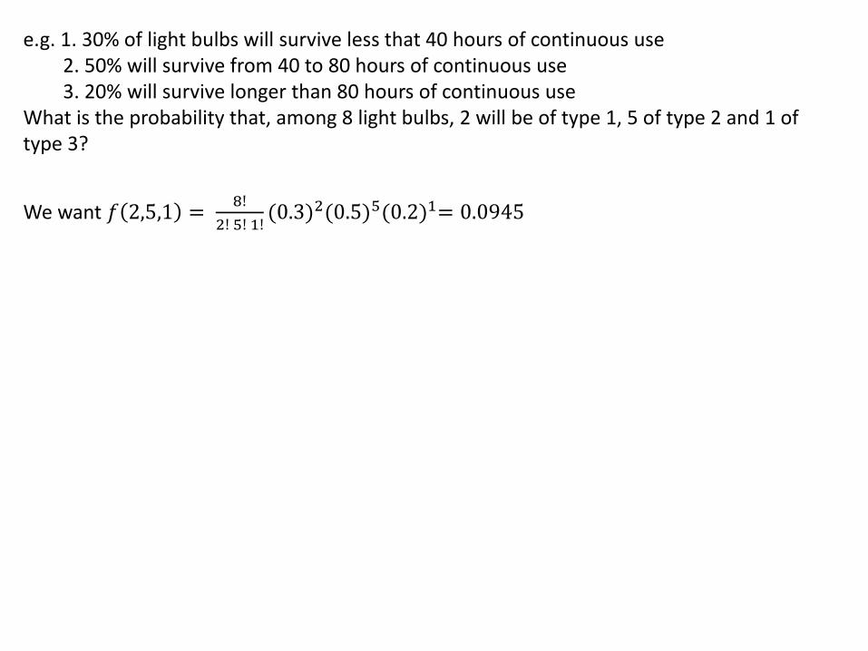
e.g. 1. 30% of light bulbs will survive less that 40 hours of continuous use 2. 50% will survive from 40 to 80 hours of continuous use 3. 20% will survive longer than 80 hours of continuous use What is the probability that, among 8 light bulbs, 2 will be of type 1, 5 of type 2 and 1 of type 3?

We want 𝑓 2,5,1 = 8!

2! 5! 1!(0.3)2(0.5)5(0.2)1= 0.0945

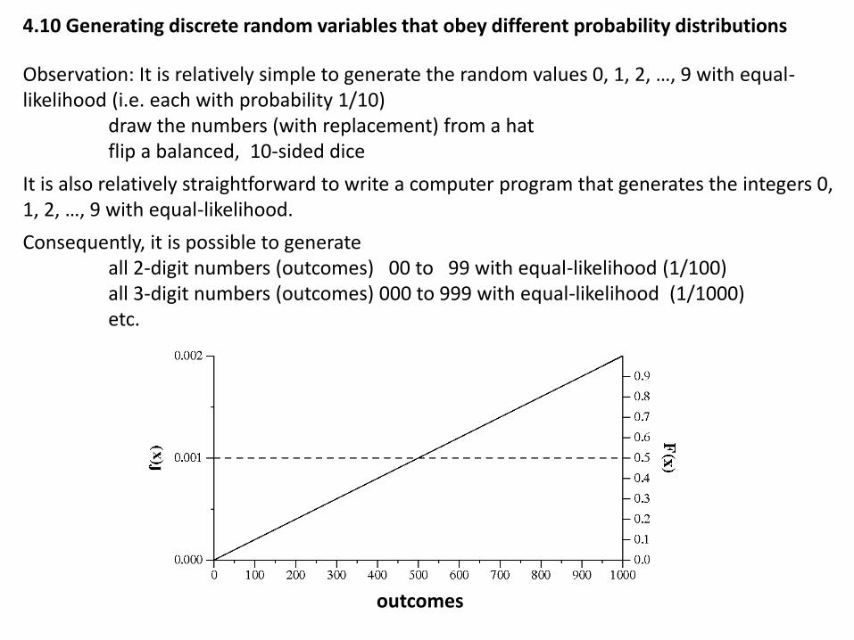
4.10 Generating discrete random variables that obey different probability distributions

Observation: It is relatively simple to generate the random values 0, 1, 2, …, 9 with equal-likelihood (i.e. each with probability 1/10) draw the numbers (with replacement) from a hat flip a balanced, 10-sided dice

It is also relatively straightforward to write a computer program that generates the integers 0, 1, 2, …, 9 with equal-likelihood.

Consequently, it is possible to generate all 2-digit numbers (outcomes) 00 to 99 with equal-likelihood (1/100) all 3-digit numbers (outcomes) 000 to 999 with equal-likelihood (1/1000) etc.

outcomes

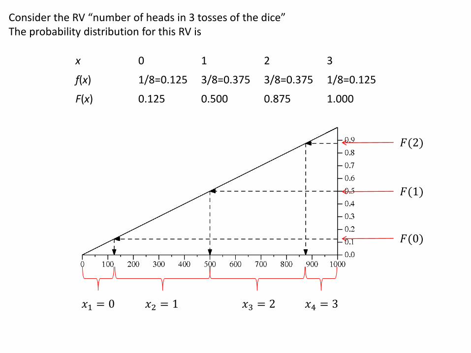
Consider the RV “number of heads in 3 tosses of the dice” The probability distribution for this RV is

x 0 1 2 3

f(x) 1/8=0.125 3/8=0.375 3/8=0.375 1/8=0.125

F(x) 0.125 0.500 0.875 1.000

𝐹(0)

𝐹(1)

𝐹(2)

𝑥1 = 0 𝑥2 = 1 𝑥3 = 2 𝑥4 = 3

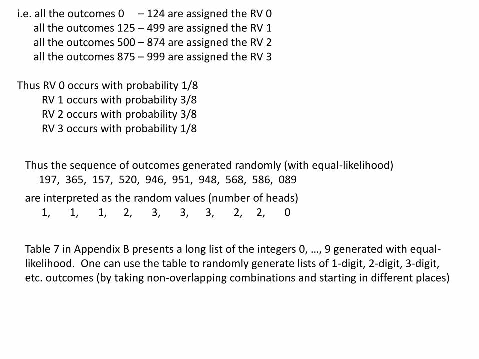
i.e. all the outcomes 0 – 124 are assigned the RV 0 all the outcomes 125 – 499 are assigned the RV 1 all the outcomes 500 – 874 are assigned the RV 2 all the outcomes 875 – 999 are assigned the RV 3 Thus RV 0 occurs with probability 1/8 RV 1 occurs with probability 3/8 RV 2 occurs with probability 3/8 RV 3 occurs with probability 1/8

Thus the sequence of outcomes generated randomly (with equal-likelihood) 197, 365, 157, 520, 946, 951, 948, 568, 586, 089

are interpreted as the random values (number of heads) 1, 1, 1, 2, 3, 3, 3, 2, 2, 0

Table 7 in Appendix B presents a long list of the integers 0, …, 9 generated with equal-likelihood. One can use the table to randomly generate lists of 1-digit, 2-digit, 3-digit, etc. outcomes (by taking non-overlapping combinations and starting in different places)

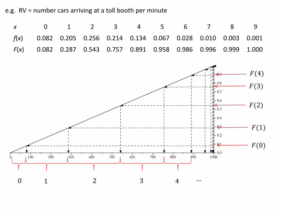
e.g. RV = number cars arriving at a toll booth per minute

x 0 1 2 3 4 5 6 7 8 9

f(x) 0.082 0.205 0.256 0.214 0.134 0.067 0.028 0.010 0.003 0.001

F(x) 0.082 0.287 0.543 0.757 0.891 0.958 0.986 0.996 0.999 1.000

𝐹(0)

𝐹(1)

𝐹(2)

0 1 2 3

𝐹(3)

𝐹(4)

4 …

Classical probability versus frequentist probability

Recall: classical probability counts outcomes and assumes all outcomes occur with equal likelihood. Frequentist probability measures the frequency of occurrence of outcomes from past “experiments”. So what do two dice really do when thrown at the same time? Classic probability: distinct (i.e. different colored) dice: There are 36 distinct outcomes, each appears with equal likelihood, therefore the (unordered) outcome 1,2 has probability 2/36

identical dice: There are 21 distinct outcomes, each appears with equal likelihood, therefore the (unordered) outcome 1,2 has probability 1/21 Frequentist probability: distinct dice: The (unordered) outcome 1,2 has measured probability 2/36 in agreement with classic probability

identical dice: The (unordered) outcome 1,2 has measured probability 2/36 (!!) in disagreement with classic probability

For identical dice, the classic view of probability for throwing two identical dice assumes all 21 outcomes occur with equal probability. This is not what occurs in practice. in practice, each of the (unordered) outcomes i, j where i ≠ j occurs more frequently than the outcomes i, i.

“Why” is the frequentist approach correct. Clearly the frequency of getting unordered outcomes cannot depend on the color of dice being thrown (i.e. the color of the dice cannot affect frequency of occurrence). Thus two identical dice must generate outcomes with the same frequency as two differently-colored dice. Note: That is not to say that the classic probability view is completely wrong. The classic view correctly counts the number of different outcomes in each case ( identical and different dice). However it computes probability incorrectly for the identical case. The frequentist view concentrates on assigning probabilities to each outcome. In the frequentist view, the number of outcomes for two identical dice is still 21, but the probabilities assigned to i,i and i,j outcomes are different.