Chapter: 4 · PDF fileDepartment of Mathematics University of Oslo Subdomain interior nodes Subdomain boundary nodes Subdomain boundaries Mek 4560 Torgeir Rusten Contents

Department ofMathematics

University of Oslo

Subdomain interior nodes

Subdomain boundary nodes Subdomain boundaries

Mek 4560Torgeir Rusten

Contents

// ..

/ .

Page 1 of 32

Go Back

Close

Quit

Chapter: 4

MEK4560The Finite Element Method in

Solid Mechanics II(February 6, 2008)

Torgeir Rusten

(E-post:[email protected])

E-post:[email protected]

E-post:[email protected]


University of Oslo




Contents

// ..

/ .

Page 2 of 32

Go Back

Close

Quit

Contents

4 Plates 34.1 Introduction to plates . . . . . . . . . . . . . . . . . . . . . . . . . . . . . . . . 54.2 Assumptions . . . . . . . . . . . . . . . . . . . . . . . . . . . . . . . . . . . . . 64.3 Kinematics . . . . . . . . . . . . . . . . . . . . . . . . . . . . . . . . . . . . . . 74.4 Moment-bending relations . . . . . . . . . . . . . . . . . . . . . . . . . . . . . . 94.5 Potential energy . . . . . . . . . . . . . . . . . . . . . . . . . . . . . . . . . . . 104.6 Equilibrium I . . . . . . . . . . . . . . . . . . . . . . . . . . . . . . . . . . . . . 114.7 Equilibrium II . . . . . . . . . . . . . . . . . . . . . . . . . . . . . . . . . . . . . 124.8 Field equations I . . . . . . . . . . . . . . . . . . . . . . . . . . . . . . . . . . . 154.9 Field equations II . . . . . . . . . . . . . . . . . . . . . . . . . . . . . . . . . . . 194.10 Boundary conditions . . . . . . . . . . . . . . . . . . . . . . . . . . . . . . . . . 214.11 Summary . . . . . . . . . . . . . . . . . . . . . . . . . . . . . . . . . . . . . . . 25

A References 32


University of Oslo




Contents

// ..

/ .

Page 3 of 32

Go Back

Close

Quit

4. Plates

The topic of the following Chapters are plate theory, both classical thin plate theory and theoryfor thick plates. While the membrane formulation is characterized by the fact that loads andresponses are in the plane, the plate models consider out of plane loads and responses.

Recall that the classical beam models are forth order differential equations, and that C1 conti-nuity is required for the finite element approximation. This is straightforward to achieve withcubic polynomials.

We will see below a model of thin plates, based on Kirchhoff theory, which also result in a forthorder differential equation. Thus, for a conforming element method C1 continuity is requiredacross inter element boundaries. In 2D this is more difficult to achieve, it turns out that fortriangular elements a quintic polynomial is required.

An alternative to thin plates are thick plates based on Mindlin-Reissner theory, similar to themodel of beams. Here C0 continuity is sufficient and the usual finite elements can be used,however the problem with shear locking is also present for plates.

In the sequel we discuss:

1. Kirchhoff plates, thin plates where transverse shear strains assumed to vanish.

2. Mindlin-Reissner plates, nonzero transverse shear strains.


University of Oslo




Contents

// ..

/ .

Page 4 of 32

Go Back

Close

Quit

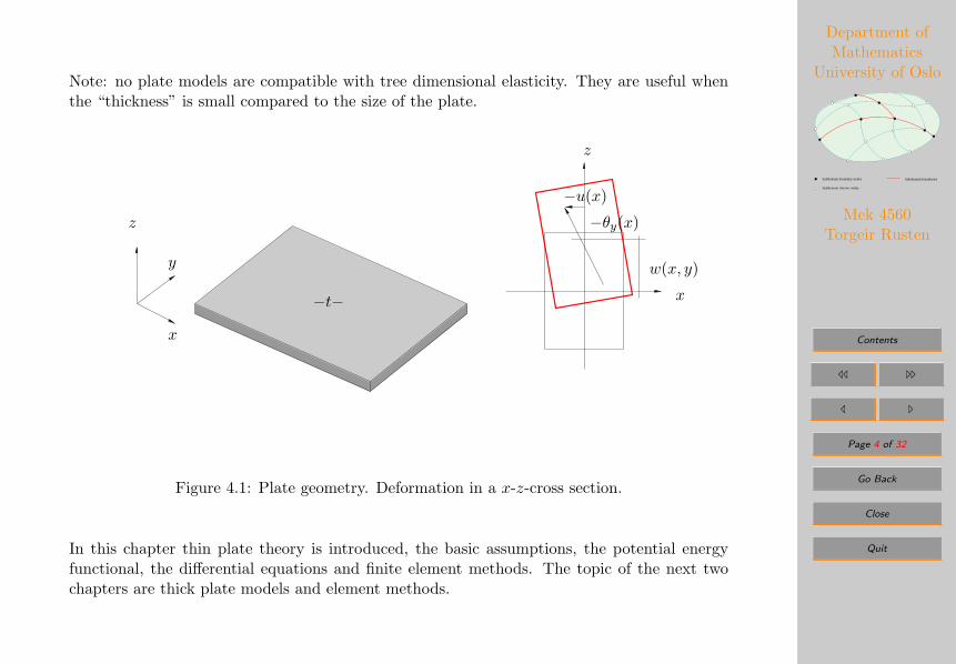
Note: no plate models are compatible with tree dimensional elasticity. They are useful whenthe “thickness” is small compared to the size of the plate.

x

y

z

−t− x

z

−u(x)

−θy(x)

w(x, y)

Figure 4.1: Plate geometry. Deformation in a x-z-cross section.

In this chapter thin plate theory is introduced, the basic assumptions, the potential energyfunctional, the differential equations and finite element methods. The topic of the next twochapters are thick plate models and element methods.


University of Oslo




Contents

// ..

/ .

Page 5 of 32

Go Back

Close

Quit

The relevant sections in the text book [Cook et al., 2002]Cook:01 are 15.1, 15.2, 15.3, 15.4 and15.5.

4.1. Introduction to plates

A plate is:

1. The geometry is plane and the “thickness” t is small compared to the “length” L.

tL > 1

3 thick plates, full three dimensional analysis.13 >

tL > 1

10 medium thick plates, analysis using thick plate theory.tL < 1

10 thin plates, thin plate theory.

2. The load is “out of plane”.

3. The response in bending; the stress throughout the thickness is not uniform.

Remark 4.1 In order to use a plate model, the thickness can not be to small, eg. kites andhot air balloons can not be analyzed using plate models.


University of Oslo




Contents

// ..

/ .

Page 6 of 32

Go Back

Close

Quit

4.2. Assumptions

The derivation of a model of thin plates are based on the following assumptions:

1. The geometry is given by:

V ={

(x, y, x) ∈ R3|(x, y) ∈ A ⊂ R2, z ∈(− t

2,t

2)}

where t is the plate thickness and A is the middle plane.

2. Transverse share strains are zero

γxz = γyz = 0

3. The stress normal to the plate midlplane are negligible

σzz = 0

4. Small rotations and small displacements:

w(x, y) << t, sinα = α =∂w

∂x

similarly for the rotations around the x-axis

5. No stress in the middle plane:

σxx = σyy = σxy = 0

The boundary conditions must be compatible to this assumption.


University of Oslo




Contents

// ..

/ .

Page 7 of 32

Go Back

Close

Quit

Remark 4.2 In general the thickness can be a function of x and y, t = t(x, y). However, thevariation must be “sufficiently” slow in order to avoid three dimensional effects.

Remark 4.3 The term inextensional bending is used when the middle-plane has zero stress.It is also called plate bending. If the the middle-plane has “sufficiently” large deformations itis called extensional bending and a shell model is appropriate.

4.3. Kinematics

Displacements: The in plane displacements are related to the normal displacements asfollows:

u(x, y, z) = −z ∂w∂x

, v(x, y, z) = −z ∂w∂y

and w(x, y, z) = w(x, y)

Thus, just as for the Euler-Bernoulli beam:

Plane cross sections remains plane and normal to the middle-plane during deformations.

Based on the above assumptions on the displacement field we can find:

• strain, stress, potential energy and equilibrium.


University of Oslo




Contents

// ..

/ .

Page 8 of 32

Go Back

Close

Quit

Strains: The strain vector is composed of in-plane strains:

ε =

εxx

εyy

γxy

=

∂∂x 0

0 ∂∂y

∂∂y

∂∂x

(u

v

)=

∂∂x 0

0 ∂∂y

∂∂y

∂∂x

(−z ∂w

∂x

−z ∂w∂y

)= −z

∂2w∂x2

∂2w∂y2

2 ∂2w∂x∂y

= −zκ(w)

where the bending vector, κ(w), is introduced:

κ(w) =

κxx(w)

κyy(w)

κxy(w)

=

∂2w∂x2

∂2w∂y2

2 ∂2w∂x∂y

Remark 4.4 Using the kinematic assumptions

εzz =∂w

∂z= 0, 2εxz = γxz =

∂u

∂z+∂w

∂x= −∂w

∂x+∂w

∂x= 0

and 2εyz = γyz =∂v

∂z+∂w

∂y= −∂w

∂y+∂w

∂y= 0

thus the requirement of vanishing transverse shear follows from the kinematic assumptions.

Remark 4.5 In the derivation of the beam theory a certain inconsistency existed. A similarinconsistency exist for plate theory.

Note that the plate theory also has certain inconsistencies, just as the beam models. Inparticular, the shear strains are zero. For an isotropic material this implies that the shear


University of Oslo




Contents

// ..

/ .

Page 9 of 32

Go Back

Close

Quit

stresses, σxz = σyz = 0, also vanish. As for the beam the shear forces are in the equilibriumequations.

The normal strains, εzz, are also zeros, i.e. we have a plane strain condition. On the otherhand, we also have σzz = 0, which more natural physical assumption. For an isotropic materialthe conditions of plane stress and plane strain implies that ν = 0.

4.4. Moment-bending relations

Stresses: The stress strain relations are found from the material law:

σ = Eε = −zEκ

In plate theory is is useful to introduce shear forces, stresses integrated across the plate thick-ness. They result in moments:

M =

Mxx

Myy

Mxy

=∫ − t

2

− t2

−σz dz =∫ − t

2

− t2

Ez2 dzκ = Dκ

E int the expression above can be a general material law, however in the following we makethe assumption of an isotropic material.

Remark 4.6 Note that the reference plane is the middle plane, thus bending is not coupledto axial deformations in the middle plane.


University of Oslo




Contents

// ..

/ .

Page 10 of 32

Go Back

Close

Quit

4.5. Potential energy

Using the above in the potential energy functional for for three dimensional elasticity, we obtainthe potential energy functional for plate bending.

The strain energy becomes:

U(w) =12

∫VσTε dV =

12

∫VεTEε dV =

12

∫A

∫ t2

− t2

z2κTEκ dz dA =12

∫Aκ(w)TDκ(w) dA

or U(w) =12

∫AMTκ(w) dA

For an isotropic and homogeneous material the internal energy becomes:

U(w) =Et3

24(1− ν2)

∫A

[(∂2w

∂x2

)2

+ 2ν(∂2w

∂x2

)(∂2w

∂y2

)

+(∂2w

∂y2

)2

+ 2(1− ν)(∂2w

∂x∂y

)2]dA (4.1)

In case the loading consist of transversal loads the load potential becomes

W (w) =∫

VF Tu dV =

∫Aqw dA


University of Oslo




Contents

// ..

/ .

Page 11 of 32

Go Back

Close

Quit

4.6. Equilibrium I

The equilibrium conditions can be derived by minimizing the potential energy functional.The minimum, or stationary value, is taken for a function w satisfying the Euler-Lagrangeequations. The functional above is of the form:

Π =∫

VF (x, y, w,w,x, w,y, w,xx, w,xy, w,yy) dV

The Euler-Lagrange equations, see [Gelfand and Fomin, 1963][2], are:

∂F

∂w− ∂

∂x

∂F

∂w,x− ∂

∂y

∂F

∂w,y+

∂2

∂x2

∂F

∂w,xx+

∂2

∂x∂y

∂F

∂w,xy+

∂2

∂y2

∂F

∂w,yy= 0

For a isotropic and homogeneous material the associated differential equations becomes

q +Et3

24(1− ν)

[∂2

∂x2(2w,xx + 2νw,yy) +

∂2

∂x∂y(4(1− ν)w,xy) +

∂2

∂y2(2w,yy + 2νw,xx)

]= q +

Et3

24(1− ν)[2w,xxxx + 2νwxxyy + 4(1− ν)w,xxyy + 2w,yyyy + 2νwxxyy]

= q +D [w,xxxx + 2w,xxyy + w,yyyy] = 0

Thus the thin plate equation is:

∂4w

∂x4+ 2

∂4w

∂x2∂y2+∂4w

∂y4= − q

D

[2] I. M. Gelfand and S. V. Fomin. Calculus of Variations. Prentice-Hall, Inc., Englewood Cliffs, New Jersey,1963.


University of Oslo




Contents

// ..

/ .

Page 12 of 32

Go Back

Close

Quit

∆∆w = − q

Dor ∆2w = − q

D

or, with a slight abuse of notation since ∇2 is taken to mean ∇ · ∇ = ∇T∇,

∇2∇2w = − q

Dor ∇4w = − q

D(4.2)

where

D =Et3

12(1− ν2)

4.7. Equilibrium II

Above we used a result from calculus of variations to derive the Euler-Lagrange equationsfor the thin plate model. Here we show how to find the minimum of the potential energyfunctionals arising in linearized elasticity.

First, consider the function

Π(V ) =12V TKV − V TF (4.3)

where V and F are vectors of dimension n and K is an n by n matrix. Think of K as thestiffness matrix, F as a load vector and V the degrees of freedom of a finite element model.Thus (4.3) is a finite element approximation of the potential energy functional.


University of Oslo




Contents

// ..

/ .

Page 13 of 32

Go Back

Close

Quit

In order to find the minimum one could compute the gradient and find the vector U where thegradient is zero. I.e. set all the partial derivatives to zeros, or

∂Π∂Vi

= 0 (4.4)

for i = 1, . . . , n.

Note that∂Π∂Vi

=[Π′(V + tei)

]t=0

(4.5)

where ei is an n vector with 1 in location i and zeroes elsewhere. Consequently, if[Π′(U + tV )

]t=0

= 0 (4.6)

for all vectors V it follows that at the point U all the partial derivatives are zero.

ButΠ(U + tV ) =

12

(UTKU + 2tV TKU + t2V TKV )− (UTF + tUTF ) (4.7)

ThusΠ′(U + tV ) = V TKU + tV TKV − V TF (4.8)

and evaluating this at t = 0 we have shown that

V T (KU − F ) = 0 for all V (4.9)

Since it holds for all V , it holds for all the unit vectors ei, thus the vector U satisfies

KU = F (4.10)


University of Oslo




Contents

// ..

/ .

Page 14 of 32

Go Back

Close

Quit

Then, we consider the continuous plate problem. In order to simplify the writing

K(w, v) =∫

Aκ(w)Dκ(v) dA and F (v) =

∫Aqv dA (4.11)

Note that K(w, v) = K(v, w) and that K(v, v) ≥ 0

Then the potential energy functional for the thin plate formulation can be written

Π(v) =12K(v, v)− F (v) (4.12)

As above the function w that minimize the potential energy functional satisfy

Π′(w + tv) = 0 (4.13)

for all v and t = 0.

Note thatF (w + tv) = F (w) + tF (v) (4.14)

andK(w + tv, w + tv) = K(w,w) + 2tK(w, v) + t2K(v, v) (4.15)

ThusΠ′(w + tv) = K(w, v) + tK(v, v)− F (v) (4.16)

and the function w minimizing Π(v) satisfies

K(w, v) = F (v) for all v (4.17)


University of Oslo




Contents

// ..

/ .

Page 15 of 32

Go Back

Close

Quit

It is beyond the scope this course to discuss the existence of a function w.

Note that (4.17) correspond to the principle of virtual work, and is called a weak formulation.

Note that the derivation is general and with suitable definition of K(w, v) and F (v) all formu-lations of linearized elasticity, e.g. three dimensional, membrane, beam, etc. is covered.

4.8. Field equations I

In order to derive the differential equation, note that the weak form of the thin plate problemis: Find w satisfying∫

AMxx(w)v,xx +Myy(w)v,yy + 2Mxy(w)v,xy dA =

∫Aq v dA for all v (4.18)

Now, the Greens formula is used to move derivatives from the test function v to the momentsM.

First∫AMxxv,xx dA =

∫∂AMxxv,xnx dS −

∫AMxx,xv,x dA

=∫

∂AMxxv,xnx dS −

∫∂AMxx,xvnx dS +

∫AMxx,xxv dA (4.19)


University of Oslo




Contents

// ..

/ .

Page 16 of 32

Go Back

Close

Quit

where nx is the x component of the unit outward normal vector. Then∫AMyyv,yy dA =

∫∂AMyyv,yny dS −

∫AMyy,yv,y dA

=∫

∂AMyyv,yny dS −

∫∂AMyy,yvny dS +

∫AMyy,yyv dA (4.20)

where ny is the y component of the unit outward normal vector.

The 2Mxyv,xy is handled similarly, for one term the Green formula is used for x first and thenfor y, for the other term it is used for y first and then for x.

Collecting the terms we obtain: Find w satisfying∫A(Mxx,xx + 2Mxy,xy +Myy,yy

)v dA+

∫∂Av,xMxxnx + v,yMyyny + v,xMxyny + v,yMxynx dS

−∫

∂Av(Mxx,xnx +Myy,yny +Mxy,ynx +Mxy,xny) dS =


In order to discuss the boundary conditions the boundary integrals is rewritten. The outwardnormal on the boundary is n and the unit tangent vector is s. Since we are in two dimensionss = (−ny, nx). First

v,xMxxnx + v,yMyyny + v,xMxyny + v,yMxynx = (∇v)T

(Mxxnx +Mxyny

Mxynx +Myyny

)(4.22)


University of Oslo




Contents

// ..

/ .

Page 17 of 32

Go Back

Close

Quit

The gradient can be decomposed into

∇v = (∇v)Tnn+ (∇v)T s s =∂v

∂nn+

∂v

∂ss (4.23)

We also introduce the notation

Mnn = nT

(Mxxnx +Mxyny

Mxynx +Myyny

)and Mns = sT

(Mxxnx +Mxyny

Mxynx +Myyny

)(4.24)

Thusv,xMxxnx + v,yMyyny + v,xMxyny + v,yMxynx =

∂v

∂nMnn +

∂v

∂sMns (4.25)

For the second term we introduce the shear forces Qx and Qy and obtain

Mxx,xnx +Myy,yny +Mxy,ynx +Mxy,xny = Qxnx +Qyny = Qn (4.26)

The weak form takes the form: Find w satisfying∫A(Mxx,xx + 2Mxy,xy +Myy,yy

)v dA

+∫

∂A

∂v

∂nMnn +

∂v

∂sMns dS −

∫∂Av Qn dS =


Now, use test functions v such that v = ∂v∂n = 0, then

Mxx,xx + 2Mxy,xy +Myy,yy = q (4.28)


University of Oslo




Contents

// ..

/ .

Page 18 of 32

Go Back

Close

Quit

Otherwise it would be possible to find a basis function that violates the equality in the weakform.

Then, assume that v = 0 on the boundary, but the normal derivative is nonzero. Since v = 0,∂v∂s = 0 and

Mnn = 0 (4.29)

To treat the final terms on the boundary we assume that the boundary is smooth and useintegration by parts ∫

∂A

∂v

∂sMns dS = −

∫∂Av∂Mns

∂sdS (4.30)

Combining this with the shear force term∫∂Av(Qn −

∂Mns

∂s

)dS = 0 (4.31)

ThusVn = Qn −

∂Mns

∂s= 0 (4.32)

The combinations of boundary conditions are summarized below. If the boundary is notsmooth corner forces enters at the corner points, see below.


University of Oslo




Contents

// ..

/ .

Page 19 of 32

Go Back

Close

Quit

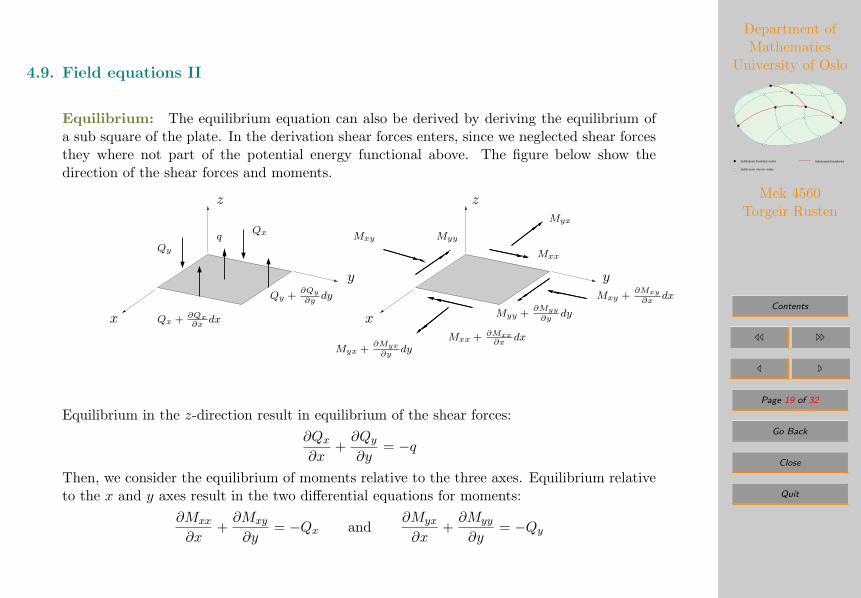
4.9. Field equations II

Equilibrium: The equilibrium equation can also be derived by deriving the equilibrium ofa sub square of the plate. In the derivation shear forces enters, since we neglected shear forcesthey where not part of the potential energy functional above. The figure below show thedirection of the shear forces and moments.

x

y

z

x

y

z

qQy

Qy +∂Qy

∂ydy

Qx

Qx + ∂Qx∂x

dx

Mxy Myy

Myx

Mxx

Myx +∂Myx

∂ydy

Mxx + ∂Mxx∂x

dx

Myy +∂Myy

∂ydy

Mxy +∂Mxy

∂xdx

Equilibrium in the z-direction result in equilibrium of the shear forces:∂Qx

∂x+∂Qy

∂y= −q

Then, we consider the equilibrium of moments relative to the three axes. Equilibrium relativeto the x and y axes result in the two differential equations for moments:

∂Mxx

∂x+∂Mxy

∂y= −Qx and

∂Myx

∂x+∂Myy

∂y= −Qy


University of Oslo




Contents

// ..

/ .

Page 20 of 32

Go Back

Close

Quit

while equilibrium relative to the z-axis result in

Mxy = Myx

This can be derived from the stresses.

Eliminating Qx, Qy and Myx result in

∂2Mxx

∂x2+ 2

∂2Mxy

∂x∂y+∂2Myy

∂y2= q

Using the material law for an isotropic material, and eliminating eliminate the moments andcurvatures, the biharmonic plate equation, Equation 4.2, can be established.


University of Oslo




Contents

// ..

/ .

Page 21 of 32

Go Back

Close

Quit

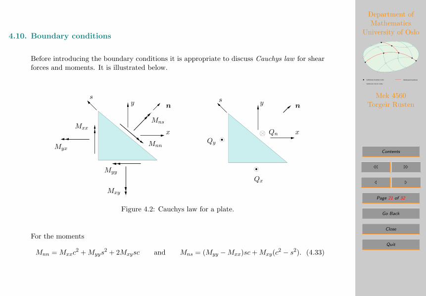
4.10. Boundary conditions

Before introducing the boundary conditions it is appropriate to discuss Cauchys law for shearforces and moments. It is illustrated below.

x

nys

x

nys

Qn

Qx

QyMyx

Mxx

Mxy

Myy

Mnn

Mns

Figure 4.2: Cauchys law for a plate.

For the moments

Mnn = Mxxc2 +Myys

2 + 2Mxysc and Mns = (Myy −Mxx)sc+Mxy(c2 − s2). (4.33)


University of Oslo




Contents

// ..

/ .

Page 22 of 32

Go Back

Close

Quit

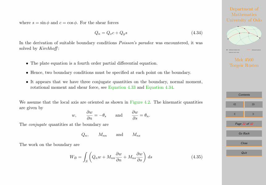
where s = sinφ and c = cosφ. For the shear forces

Qn = Qxc+Qys (4.34)

In the derivation of suitable boundary conditions Poisson’s paradox was encountered, it wassolved by Kirchhoff :

• The plate equation is a fourth order partial differential equation.

• Hence, two boundary conditions must be specified at each point on the boundary.

• It appears that we have three conjugate quantities on the boundary, normal moment,rotational moment and shear force, see Equation 4.33 and Equation 4.34.

We assume that the local axis are oriented as shown in Figure 4.2. The kinematic quantitiesare given by

w,∂w

∂n= −θs and

∂w

∂s= θn.

The conjugate quantities at the boundary are

Qn, Mnn and Mns

The work on the boundary are

WB =∫

S

(Qnw +Mnn

∂w

∂n+Mns

∂w

∂s

)ds (4.35)


University of Oslo




Contents

// ..

/ .

Page 23 of 32

Go Back

Close

Quit

It seem like we should specify three values at each point of the boundary:

Simply supported: w = 0,∂w

∂s= 0 and Mnn = 0.

Free: Qn = 0, Mnn = 0 and Mns = 0.

However, if w = 0 it follows that ∂w∂s = 0, thus only two quantities are relevant in the first case.

The reduction to two independent variables on the boundary is based on integration by partsof the middle term of Equation 4.35 along a line segment AB

WB|BA =∫

[A,B]

[(Qn −

∂Mns

∂s

)w +Mnn

∂w

∂n

]ds+Mnsw|BA

Upon introducing the modified shear force

Vn = Qn −∂Mns

∂s

the load potential can be written

WB|BA =∫

S

(Vnw +Mnn

∂w

∂n

)ds+Mnsw|BA (4.36)

This result in the correct number of conjugated quantities at the boundary:

w, Vn and∂w

∂n= −θs, Mnn


University of Oslo




Contents

// ..

/ .

Page 24 of 32

Go Back

Close

Quit

Homogeneous boundary conditions: The homogeneous boundary conditions for a thinplate is:

Clamped: w = 0 and∂w

∂n= 0.

Simply supported: w = 0 and Mnn = 0.Free: Vn = 0 and Mnn = 0.

Symmetric about s: Vn = 0 and∂w

∂n= 0.

Corner forces: The last term in Equation 4.36 needs to be explained.

If the boundary is smooth, Mns is continuous on the boundary S and that the boundary issmooth such that A = B

Mnsw|BA = 0.

In case the plate has corners, the integration is done “edge by edge”. In an corder C themoment Mns has a jump, say from M+

ns to M−ns. At the corners the jump term becomes

Mnsw|BA = Rcw = (M+ns −M−ns)w

since w is continuous. This jump is called corner forces.


University of Oslo




Contents

// ..

/ .

Page 25 of 32

Go Back

Close

Quit

4.11. Summary

In summary:

The highest derivative m in the PMPE 2

Highest derivative 2m (in the differential equation) 4

Kinematic boundary conditions (0, 1) (w,w,n = −θs)

Natural boundary condition (2, 3) (Mnn, Vn)

Continuity requirement m− 1 1 (w,w,x, w,y)

The load potential can be added to the potential energy functional:

Π(w) =12

∫AκTDκ dA−

∫Aqw dA−

∫S

(Vnw +Mnn

∂w

∂n

)ds−Mnsw|BA

Thus, distributed loads, boundary moments and boundary shear forces can be specified.

Since second derivatives are present in the formulation, C1 continuity is required for conformingfinite element methods. Unfortunately, this i more difficult in two dimensions, for a triangularelement quintic polynomials are required.

Kinematic boundary conditions are prescribed for displacements and rotations. Natural bound-ary conditions for moments and shear forces.

Before discussing finite elements for thin plates we will derive equations for thick plates.


University of Oslo




Contents

// ..

/ .

Page 26 of 32

Go Back

Close

Quit

Remark 4.7 Other sources for information on plate theory is Professor Carlos Felippa, Uni-versity of Colorado, Boulder. The notes to Advanced Finite Element Method has two chapterson plates.

A classical reference to plates is [Timoshenko and Woinowsky-Krieger, 1970][3].

[3] Stephen P. Timoshenko and S. Woinowsky-Krieger. Theory of plates and shells. Mc Graw Hill, secondedition, 1970.

http://www.colorado.edu/engineering/CAS/courses.d/AFEM.d/Home.html


University of Oslo




Contents

// ..

/ .

Page 27 of 32

Go Back

Close

Quit

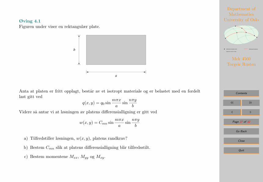
Øving 4.1Figuren under viser en rektangulær plate.

b

a

Anta at platen er fritt opplagt, bestar av et isotropt materiale og er belastet med en fordeltlast gitt ved

q(x, y) = q0 sinmπx

asin

nπy

b

Videre sa antar vi at løsningen av platens differensialligning er gitt ved

w(x, y) = Cmn sinmπx

asin

nπy

b

a) Tilfredstiller løsningen, w(x, y), platens randkrav?

b) Bestem Cmn slik at platens differensialligning blir tilfredsstilt.

c) Bestem momentene Mxx, Myy og Mxy.


University of Oslo




Contents

// ..

/ .

Page 28 of 32

Go Back

Close

Quit

d) Plot Mxy f.eks. i MATLAB. Kan du ut i fra figuren og definisjonen av Mns avgjøre om vifar hjørnekrefter i platen?

Anta at lasten na kan beskrives ved

q(x, y) =∞∑

m=1

∞∑n=1

qmn sinmπx

asin

nπy

b

For en jevnt fordelt last, q0, sa har vi at

qmn =16q0π2mn

.

Pa samme mate sa antar vi at forskyvningen er bestemt ved

w(x, y) =∞∑

m=1

∞∑n=1

Cmn sinmπx

asin

nπy

b

e) Benytt løsningen funnet for Cmn i b) over til a bestemme hver av koeffisientene Cmn.

f) Bestem hvor mange ledd i summen en trenger for a fa fire siffers nøyaktighet.

g) Gjør det samme for momentene. Konvergerer disse like fort som forskyvningen?

Øving 4.2I denne oppgaven skal vi modellere platen i oppgave 4.1 i ANSYS. Benytt q0 = 1, a = b = 10,E = 10.92, ν = 0.3 og t = 0.1.


University of Oslo




Contents

// ..

/ .

Page 29 of 32

Go Back

Close

Quit

• Modeller hele platen ved a benytte SHELL63 (KEYOPT(1) = 2, slar av membran effekter).

• Sammenlign resultatene for wmidt for elementinndelingene 2× 2, 4× 4, 8× 8 og 16× 16med eksakt løsning.

• Se pa reaksjonskreftene for 16×16 elementnettet. Kan vi se om vi har hjørnekrefter (sliksom teorien sier).

• Benytt samme element men lag et elementnett bestaende av trekanter. Sammenligntrekant- og firkantløsningen.

• Benytt symmetriegenskapene til a modeller en kvart modell. Sammenlign trekantløsningenmed trekantløsningen fra en full modell.

Øving 4.3Tynne plater er ikke tilgjengelig i COMSOL Multiphysics Structural Module. Vi kan benytteMindlin-Reissner formuleringen og sørge for at platen er tynn og sa se om vi far resultater somsamsvarer med tynnplateløsningen.


University of Oslo




Contents

// ..

/ .

Page 30 of 32

Go Back

Close

Quit

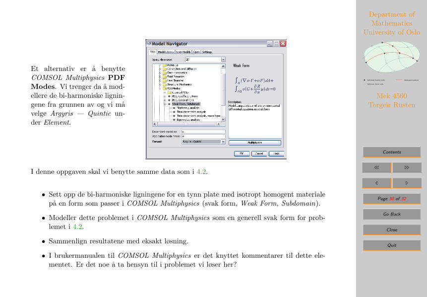
Et alternativ er a benytteCOMSOL Multiphysics PDFModes. Vi trenger da a mod-ellere de bi-harmoniske lignin-gene fra grunnen av og vi mavelge Argyris — Quintic un-der Element.

I denne oppgaven skal vi benytte samme data som i 4.2.

• Sett opp de bi-harmoniske ligningene for en tynn plate med isotropt homogent materialepa en form som passer i COMSOL Multiphysics (svak form, Weak Form, Subdomain).

• Modeller dette problemet i COMSOL Multiphysics som en generell svak form for prob-lemet i 4.2.

• Sammenlign resultatene med eksakt løsning.

• I brukermanualen til COMSOL Multiphysics er det knyttet kommentarer til dette ele-mentet. Er det noe a ta hensyn til i problemet vi løser her?


University of Oslo




Contents

// ..

/ .

Page 31 of 32

Go Back

Close

Quit

• Sammenlign med resultatene fra ANSYS 10.0.

• Benytt ogsa svak formulering for de kinematiske randkravene (Lagrange — Linear inter-polasjon for de kontinuerlige Lagrange multpilikatorene). Hvordan ser disse Lagrange-multiplikatorene ut i hjørene? Tegn randverdiene.


University of Oslo




Contents

// ..

/ .

Page 32 of 32

Go Back

Close

Quit

A. References

[Cook et al., 2002] Cook, R. D., Malkus, D. S., Plesha, M. E., and Witt, R. J. (2002). Conceptsand Applications of Finite Element Analysis. Number ISBN: 0-471-35605-0. John Wiley &Sons, Inc., 4th edition.

[Gelfand and Fomin, 1963] Gelfand, I. M. and Fomin, S. V. (1963). Calculus of Variations.Prentice-Hall, Inc., Englewood Cliffs, New Jersey.

[Timoshenko and Woinowsky-Krieger, 1970] Timoshenko, S. P. and Woinowsky-Krieger, S.(1970). Theory of plates and shells. Mc Graw Hill, second edition.

Documents

Chapter: 4 · PDF fileDepartment of Mathematics University of Oslo Subdomain interior nodes Subdomain boundary nodes Subdomain boundaries Mek 4560 Torgeir Rusten Contents