123

Chapter 4

BUILDING ON THE COUNTERCYCLICAL CAPITAL BUFFERCONSENSUS: ASIAN EMPIRICAL TEST

ByChuah Lay Lian 1,2

1. Introduction

Basel III introduced a countercyclical capital buffer (CCCB) in 2010 to thebanking sector regulatory framework and it is aimed at strengthening the banks’defences against the build-up of systemic risks. Specifically, the countercyclicalcapital buffer is meant to protect the banks from periods of excessive creditgrowth, which have often been associated with systemic risks. It works assuch that a buffer of regulatory capital will be built up during a credit up cycleperiod and will be released thereby easing the constraints on the flow of creditin the economy during a credit down cycle. In doing so, the CCCB reducesthe procyclicality of credit that can amplify the credit cycle though periods ofboom and bust and in turn, reduces the build-up of financial vulnerabilities.

While periods of rapid credit expansions tend to be associated with a build-up in financial and macroeconomics instability, credit can grow rapidly for threereasons: (i) financial deepening, which is seen to support economic growth; (ii)driven by factors of demand and supply of the credit market and; (iii) excessivecyclical fluctuations such as credit booms. Therefore, the question arising fromthese reasons is that, is rapid credit growth necessarily a strong signal for growingfinancial imbalances that will typically lead to a financial crisis. Although, evidencefrom Elekdag and Wu (2011) show that Asian credit booms have beencharacterised by a higher incidences of crisis, the link between rapid creditexpansion and crisis need to be further examined before deciding the threshold

________________1. Senior Economist, Economics Department, Bank Negara Malaysia, Email:

llchuah@bnm.gov.my. This paper is still work in progress by the author and is circulatedto elicit comments and further debate. Any views expressed are solely those of the authorand so cannot be taken to represent those of Bank Negara Malaysia. This paper shouldtherefore not be reported as representing the views of Bank Negara Malaysia.

2. The author is grateful to Michael Zamorski (Financial Stability and Supervision Advisorto Bank Negara Malaysia), Zach Thor, Karen Lee, Nik Ahmad Rusydan Nik Hafizi (FinancialSurveillance Department), Roy Lim and Mohammad Aidil Mat Aris (Prudential FinancialPolicy Department) for their comments.

124

for too much or too little credit. As Edge and Meisenzahl (2011) and Buncicand Melecky (2013) point out the credit-to GDP gap, the measure recommendedby Basel III may not necessarily reflect the equilibrium level of credit for aneconomy.

The aim of this paper is to examine the reliability of the credit-to-GDP gapin signalling financial imbalances for Malaysia. The motivation of this analysisis to determine the suitability of Basel III’s recommendation in using the Hodrick-Prescott (HP) filter to derive the credit-to-GDP gap which is then used as abenchmark to determine excessive credit levels in the economy. The HP methodmay not be ideal as it is sensitive to the choice of the smoothening parameter(ë), susceptible to end point bias and lacks economic fundamentals. Given theweakness in this approach and in using the credit-to-GDP as an indicator forfinancial distress, the Basel Committee allows regulators to exercise discretionand specify different methods for setting the benchmark and appropriate thresholdsfor countercyclical capital buffers (CCCB). Therefore, this paper will also assessthe feasibility of using other key macroprudential indicators as anchors for theCCCB.

The structure of the paper is as follows. Section 2 provides the backdropfor the paper by examining the rationale behind Basel III’s recommendationwith regards to CCCB and the risks associated with excessive credit expansion.This section also discusses the phase-in schedule of Basel III for Malaysia, andthe credit trends as well as the financial soundness of the banking system ofthe country vis-a-vis other regional countries. Section 3 examines the literatureon the risks of excessive credit expansion and the role of credit-to-GDP as aforward-looking indicator for financial imbalances. Section 4 takes a closerlook at using the HP method to decompose the credit-to-GDP series into trendand cycle; and examine the usefulness of the credit-to GDP gap in identifyingperiods of a build-up in financial imbalances. This section will also examineother possible macro indicators that meet the information requirement for CCCBsetting decisions and the two methodologies in identifying appropriate thresholdsfor buffer decisions, namely (i) Sarel’s (1996) approach and; (ii) the noise-to-signal ratio approach. Section 5 discusses the empirical results of the two mainapproaches in the identification of suitable thresholds. Finally, Section 6 includespolicy recommendations and conclusions.

125

2. Comparative Evidence

2.1 The Rationale behind Basel III

The main cause of the Global Financial Crisis (GFC) in 2007-2009 can betraced back to the build-up of excessive optimism, resulting from a period ofworld-wide high economic growth, low real interest rates and subdued volatilityof financial prices as well as the flood of liquidity (Morgan and Pontines, 2013).The International Monetary Policy highlighted that macroeconomic policies didnot take into account the build-up in systemic risks as they failed to detect thethreat of a growing asset price bubble. In this context, the US Federal Reserveunderestimated the build-up of financial imbalances that emerged from housingprice bubbles, the proliferation of unsound credit practices, in particular subprimeloans to borrowers and the highly leveraged financial institutions which wasfurther aggravated by the interconnections of financial markets3.

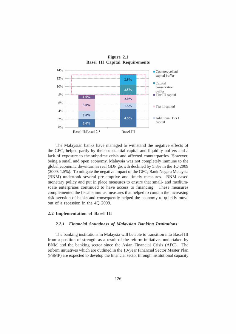
As a result of the GFC, certain shortcomings of the Basel II regulatoryframework were identified. Most banks that failed, or nearly failed were typically“well-capitalised” at that time. However, the systemic contagion highlighted theneed for global capital standards to be harmonised. Also, the events which ledto losses in the banking sector evoked debates on role of excessive credit indestabilising the banking sector and exacerbating the downturn in the realeconomy4. The debates are premised on observations that a financial crisis isusually preceded by periods of excess credit growth. The vicious cycle ofexcessive credit growth is further reinforced when the financial crisis spills overto the real economic, causes a recession which later feedbacks into the bankingsector. The interconnectedness of financial markets and institutions acrosscountries and the global macroeconomic financial links increases the systemicrisk and therefore, underscores the importance of the banking sector in buildingup its capital defences during periods when credit has grown to excessive levels.As capital is more expensive than other forms of funding, the building up ofthese defences is expected have the additional benefit of helping to dampenpro-cyclical credit growth (Figure 2.1).

________________3. The Fed was inclined not to lean against emerging asset bubbles, as it believed that such

bubbles were difficult to identify, and that it could move swiftly to clean up the damageafterward (Morgan and Pontines, 2013).

4. BCBS (2010), Elekdag and Wu (2011) and Reinhart and Rogoff (2009).

126

The Malaysian banks have managed to withstand the negative effects ofthe GFC, helped partly by their substantial capital and liquidity buffers and alack of exposure to the subprime crisis and affected counterparties. However,being a small and open economy, Malaysia was not completely immune to theglobal economic downturn as real GDP growth declined by 5.8% in the 1Q 2009(2009: 1.5%). To mitigate the negative impact of the GFC, Bank Negara Malaysia(BNM) undertook several pre-emptive and timely measures. BNM easedmonetary policy and put in place measures to ensure that small- and medium-scale enterprises continued to have access to financing. These measurescomplemented the fiscal stimulus measures that helped to contain the increasingrisk aversion of banks and consequently helped the economy to quickly moveout of a recession in the 4Q 2009.

2.2 Implementation of Basel III

2.2.1 Financial Soundness of Malaysian Banking Institutions

The banking institutions in Malaysia will be able to transition into Basel IIIfrom a position of strength as a result of the reform initiatives undertaken byBNM and the banking sector since the Asian Financial Crisis (AFC). Thereform initiatives which are outlined in the 10-year Financial Sector Master Plan(FSMP) are expected to develop the financial sector through institutional capacity

Figure 2.1Basel III Capital Requirements

127

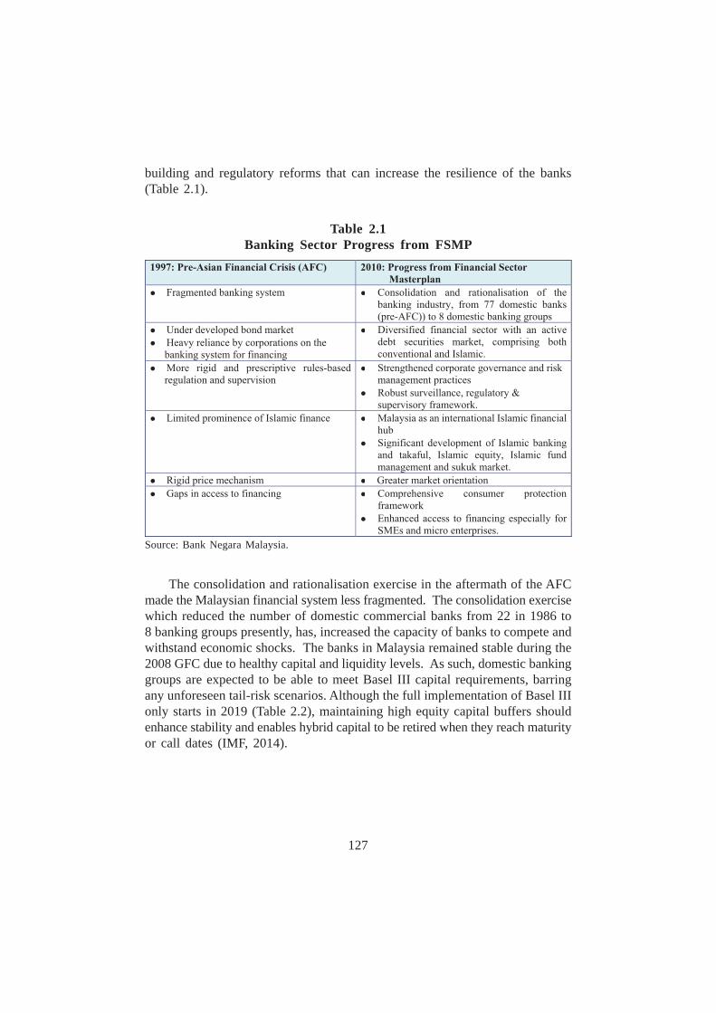
building and regulatory reforms that can increase the resilience of the banks(Table 2.1).

The consolidation and rationalisation exercise in the aftermath of the AFCmade the Malaysian financial system less fragmented. The consolidation exercisewhich reduced the number of domestic commercial banks from 22 in 1986 to8 banking groups presently, has, increased the capacity of banks to compete andwithstand economic shocks. The banks in Malaysia remained stable during the2008 GFC due to healthy capital and liquidity levels. As such, domestic bankinggroups are expected to be able to meet Basel III capital requirements, barringany unforeseen tail-risk scenarios. Although the full implementation of Basel IIIonly starts in 2019 (Table 2.2), maintaining high equity capital buffers shouldenhance stability and enables hybrid capital to be retired when they reach maturityor call dates (IMF, 2014).

Table 2.1Banking Sector Progress from FSMP

Source: Bank Negara Malaysia.

128

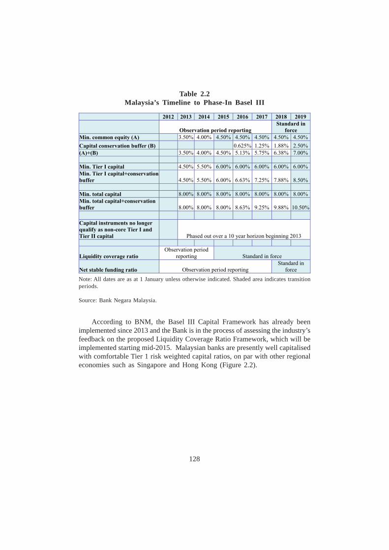
According to BNM, the Basel III Capital Framework has already beenimplemented since 2013 and the Bank is in the process of assessing the industry’sfeedback on the proposed Liquidity Coverage Ratio Framework, which will beimplemented starting mid-2015. Malaysian banks are presently well capitalisedwith comfortable Tier 1 risk weighted capital ratios, on par with other regionaleconomies such as Singapore and Hong Kong (Figure 2.2).

Note: All dates are as at 1 January unless otherwise indicated. Shaded area indicates transitionperiods.

Source: Bank Negara Malaysia.

Table 2.2Malaysia’s Timeline to Phase-In Basel III

129

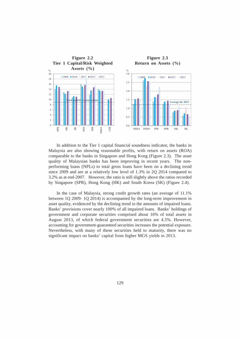
Figure 2.2Tier 1 Capital/Risk Weighted

Assets (%)

Figure 2.3Return on Assets (%)

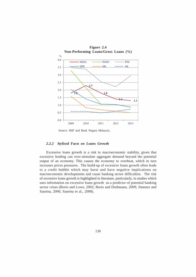
In addition to the Tier 1 capital financial soundness indicator, the banks inMalaysia are also showing reasonable profits, with return on assets (ROA)comparable to the banks in Singapore and Hong Kong (Figure 2.3). The assetquality of Malaysian banks has been improving in recent years. The non-performing loans (NPLs) to total gross loans have been on a declining trendsince 2009 and are at a relatively low level of 1.3% in 2Q 2014 compared to3.2% as at end-2007. However, the ratio is still slightly above the ratios recordedby Singapore (SPR), Hong Kong (HK) and South Korea (SK) (Figure 2.4).

In the case of Malaysia, strong credit growth rates (an average of 11.1%between 1Q 2009- 1Q 2014) is accompanied by the long-term improvement inasset quality, evidenced by the declining trend in the amounts of impaired loans.Banks’ provisions cover nearly 100% of all impaired loans. Banks’ holdings ofgovernment and corporate securities comprised about 16% of total assets inAugust 2013, of which federal government securities are 4.5%. However,accounting for government-guaranteed securities increases the potential exposure.Nevertheless, with many of these securities held to maturity, there was nosignificant impact on banks’ capital from higher MGS yields in 2013.

130

2.2.2 Stylised Facts on Loans Growth

Excessive loans growth is a risk to macroeconomic stability, given thatexcessive lending can over-stimulate aggregate demand beyond the potentialoutput of an economy. This causes the economy to overheat, which in turnincreases prices pressures. The build-up of excessive loans growth often leadsto a credit bubble which may burst and have negative implications onmacroeconomic developments and cause banking sector difficulties. The riskof excessive loans growth is highlighted in literature, particularly, in studies whichuses information on excessive loans growth as a predictor of potential bankingsector crises (Borio and Lowe, 2002; Borio and Drehmann, 2009; Jimenez andSaurina, 2006; Saurina et al., 2008).

%

Figure 2.4Non-Performing Loans/Gross Loans (%)

Source: IMF and Bank Negara Malaysia.

131

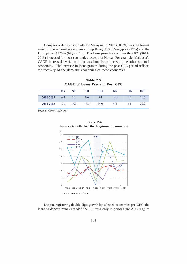
Comparatively, loans growth for Malaysia in 2013 (10.6%) was the lowestamongst the regional economies - Hong Kong (16%), Singapore (17%) and thePhilippines (15.7%) (Figure 2.4). The loans growth rates after the GFC (2011-2013) increased for most economies, except for Korea. For example, Malaysia’sCAGR increased by 4.1 ppt, but was broadly in line with the other regionaleconomies. The increase in loans growth during the post-GFC period reflectsthe recovery of the domestic economies of these economies.

Table 2.3CAGR of Loans Pre- and Post GFC

Source: Haver Analytics.

Figure 2.4Loans Growth for the Regional Economies

Source: Haver Analytics.

Despite registering double digit growth by selected economies pre-GFC, theloans-to-deposit ratio exceeded the 1.0 ratio only in periods pre-AFC (Figure

132

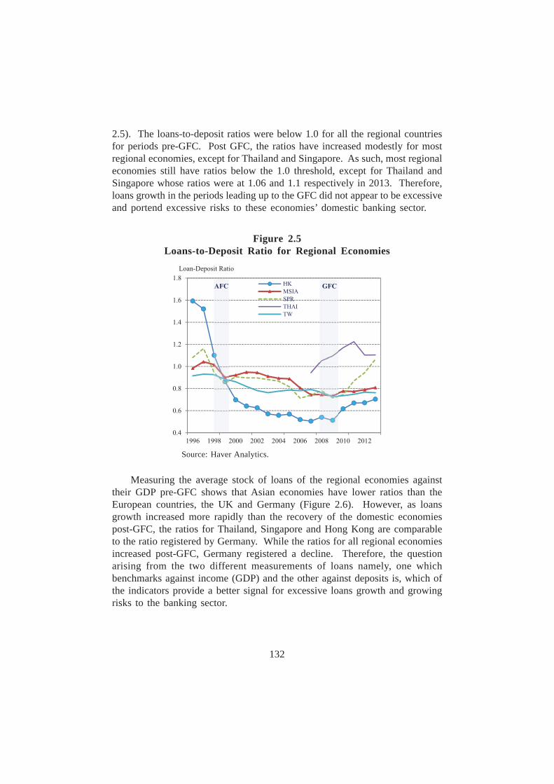
2.5). The loans-to-deposit ratios were below 1.0 for all the regional countriesfor periods pre-GFC. Post GFC, the ratios have increased modestly for mostregional economies, except for Thailand and Singapore. As such, most regionaleconomies still have ratios below the 1.0 threshold, except for Thailand andSingapore whose ratios were at 1.06 and 1.1 respectively in 2013. Therefore,loans growth in the periods leading up to the GFC did not appear to be excessiveand portend excessive risks to these economies’ domestic banking sector.

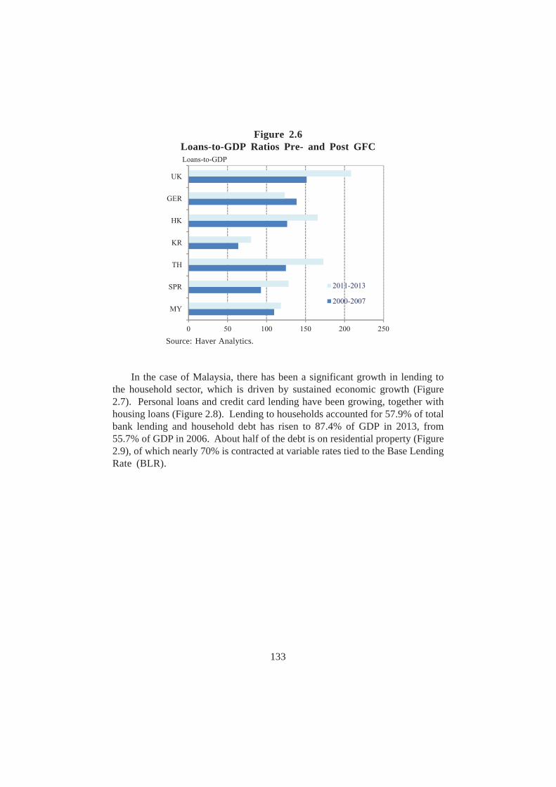
Measuring the average stock of loans of the regional economies againsttheir GDP pre-GFC shows that Asian economies have lower ratios than theEuropean countries, the UK and Germany (Figure 2.6). However, as loansgrowth increased more rapidly than the recovery of the domestic economiespost-GFC, the ratios for Thailand, Singapore and Hong Kong are comparableto the ratio registered by Germany. While the ratios for all regional economiesincreased post-GFC, Germany registered a decline. Therefore, the questionarising from the two different measurements of loans namely, one whichbenchmarks against income (GDP) and the other against deposits is, which ofthe indicators provide a better signal for excessive loans growth and growingrisks to the banking sector.

Figure 2.5Loans-to-Deposit Ratio for Regional Economies

Source: Haver Analytics.

133

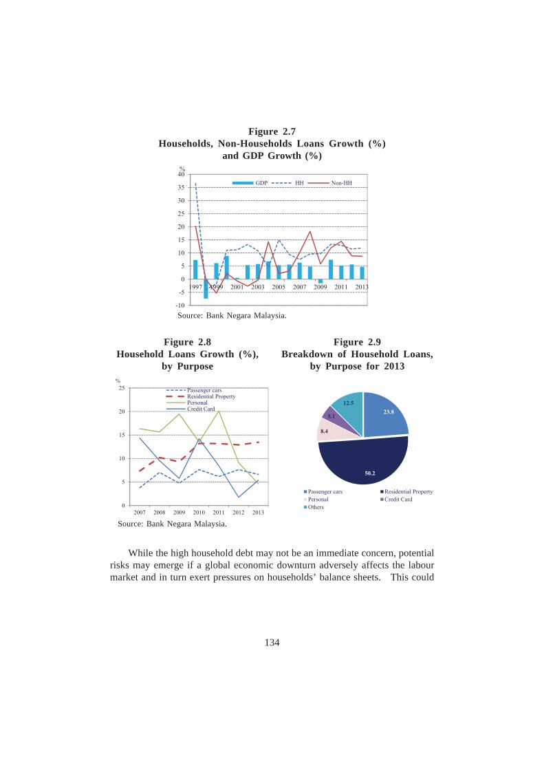
In the case of Malaysia, there has been a significant growth in lending tothe household sector, which is driven by sustained economic growth (Figure2.7). Personal loans and credit card lending have been growing, together withhousing loans (Figure 2.8). Lending to households accounted for 57.9% of totalbank lending and household debt has risen to 87.4% of GDP in 2013, from55.7% of GDP in 2006. About half of the debt is on residential property (Figure2.9), of which nearly 70% is contracted at variable rates tied to the Base LendingRate (BLR).

Figure 2.6Loans-to-GDP Ratios Pre- and Post GFC

Source: Haver Analytics.

134

While the high household debt may not be an immediate concern, potentialrisks may emerge if a global economic downturn adversely affects the labourmarket and in turn exert pressures on households’ balance sheets. This could

Figure 2.7Households, Non-Households Loans Growth (%)

and GDP Growth (%)

Figure 2.8Household Loans Growth (%),

by Purpose

Figure 2.9Breakdown of Household Loans,

by Purpose for 2013

Source: Bank Negara Malaysia.

Source: Bank Negara Malaysia.

135

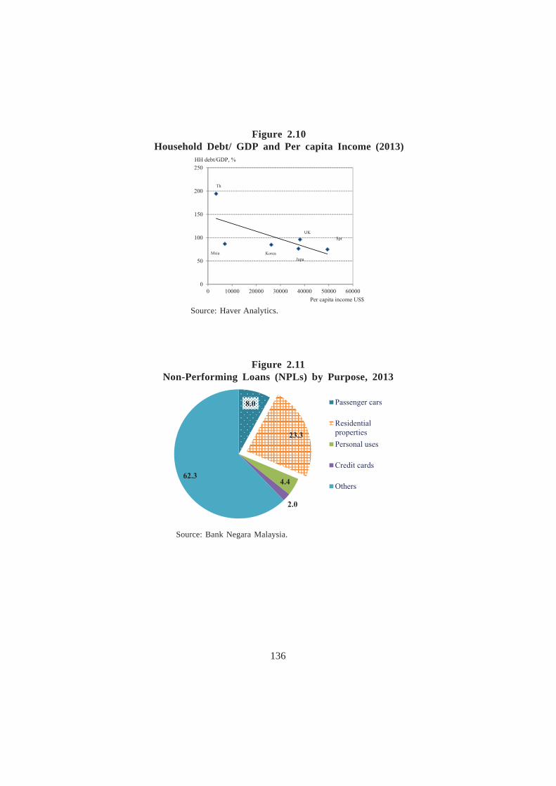
weaken household’s ability to service their loans and in turn deteriorate the assetquality of financial institutions5. Over the past 10 years, the ratio of householddebt-to-GDP has been on an increasing trend. Household debt-to-GDP in 2013appears to be at similar levels to that of advanced countries with higher percapita income (Figure 2.10). However, the rising trend in household debt coincidedwith a growing economy, stable employment conditions and rising income levels.According to Bank Negara Malaysia6, household financial buffers are atcomfortable levels as the growth in household debt has generally beenaccompanied by a corresponding expansion in households’ financial assets.Households’ financial assets as at 2013 was about 2.2 times of their debts andabout 60% of these debts were backed by deposits.

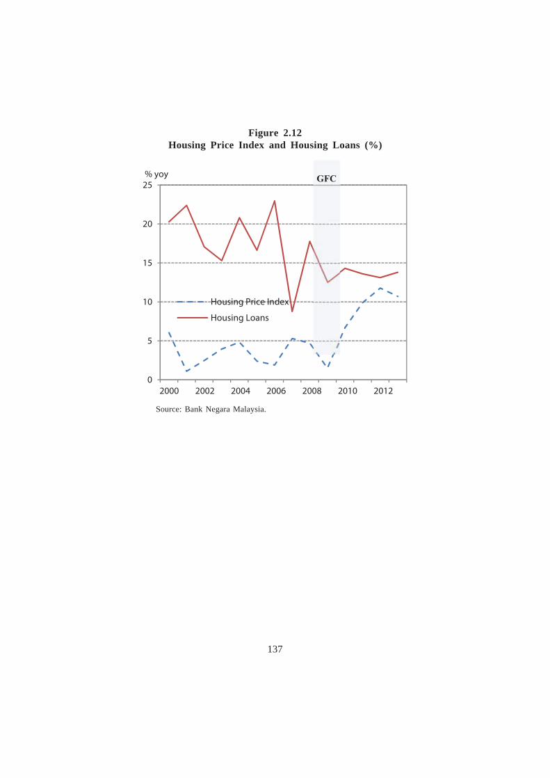
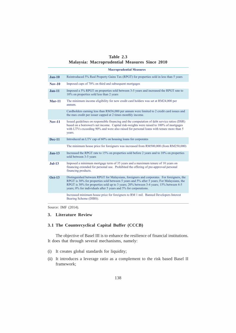
The non-performing loans (NPLs) to households accounted for 39.2% oftotal NPLs in 2013 and the rest was from lending to the business sector. Withinthe household sector, borrowings is concentrated in the residential properties(23%) followed by passenger cars (8%) (Figure 2.11). As about half of thehousehold debts are tied to the housing market, the potential risks of thespeculative purchases of residential properties was pre-empted by a series ofmacroprudential policies. Beginning November 2010 and in the 2014 budget,the authorities have imposed a series of targeted and gradual macroprudentialpolicies directed at speculative purchases of homes and unsecured credit (Table2.3). There appears to be some signs that the more recent measures haveslowed down the approval of new loans and begun to cool the housing market(Figure 2.12). If credit growth remains strong, additional macroprudential policiesmay be needed, and the scope and stringency would depend on the evolvingstance of monetary policy.

________________5. Evidence from the studies by the IMF show that economic downturns tend to be more

severe when they are preceded by significant build-ups in household debts.

6. Bank Negara indicated that further efforts have been made to enhance data collection onhouseholds. This will enable the Bank to conduct a more granular and robust assessmenton households’ debt position by income category.

136

Figure 2.11Non-Performing Loans (NPLs) by Purpose, 2013

Figure 2.10Household Debt/ GDP and Per capita Income (2013)

Source: Haver Analytics.

Source: Bank Negara Malaysia.

137

Figure 2.12Housing Price Index and Housing Loans (%)

Source: Bank Negara Malaysia.

138

Table 2.3Malaysia: Macroprudential Measures Since 2010

Source: IMF (2014).

3. Literature Review

3.1 The Countercyclical Capital Buffer (CCCB)

The objective of Basel III is to enhance the resilience of financial institutions.It does that through several mechanisms, namely:

(i) It creates global standards for liquidity;

(ii) It introduces a leverage ratio as a complement to the risk based Basel IIframework;

139

(iii) It raises the quantity, quality, consistency and transparency of Tier I capitalbase;

(iv) It introduces capital conservation buffer of 2.5% of risk-weighted assets,which is above the minimum capital requirement; and

(v) It introduces countercyclical capital buffer, ranging from 0-2.5% of risk-weighted assets.

The countercyclical capital buffer (CCCB) extends the newly introducedcapital conservation buffer by up to 2.5% of risk-weighted assets during periodsof excess credit growth associated with an increase in system wide risk. TheCCCB and the conservation buffer share the same objective which is, to buildup adequate buffers above the minimum so that it can be drawn down duringperiods of stress. For the CCCB, Basel III requires the authorities to monitorcredit growth and other indicators that may signal a build-up in systematic widerisk. The idea behind CCCB is that it wants to ensure that the banks haveadequate capital to maintain the flow of credit in the economy during thecorrection period of financial imbalances caused by excessive credit growth.

The CCCB helps to offset the frequency and the extent of credit boomsby requiring banks to build-up capital buffers during periods of excessive creditgrowth. The opposite action is required from the banks during periods of creditbust, consequently easing the constraints on the flow of credit in the economyduring periods of economic difficulties. The countercyclical action of capitalbuffer decisions moderates the inherent pro-cyclicality of the financial systemand, hence, reduces the likelihood of a bust by arresting the build-up of a system-wide risk.

The Basel III framework allows the authorities to use their discretion onwhen to activate the CCCB and the size of the buffer during the period ofexcessive credit and increasing system-wide risk. Decisions on the buffer add-on would be announced a year in advance to give banks time to react butreductions in the buffer could take place immediately. The consequences of abank’s capital falling below the level set by the countercyclical capital bufferwill be similar to the conservation buffer, where the constraints on distributiveearnings for the banks will become binding.

The Basel III framework proposes a methodology to calculate aninternationally consistent buffer guide that serves as a common reference pointfor making buffer decisions. The framework suggests the use of the credit-to-GDP gap as an indicator to guide the authorities on whether to increase or

140

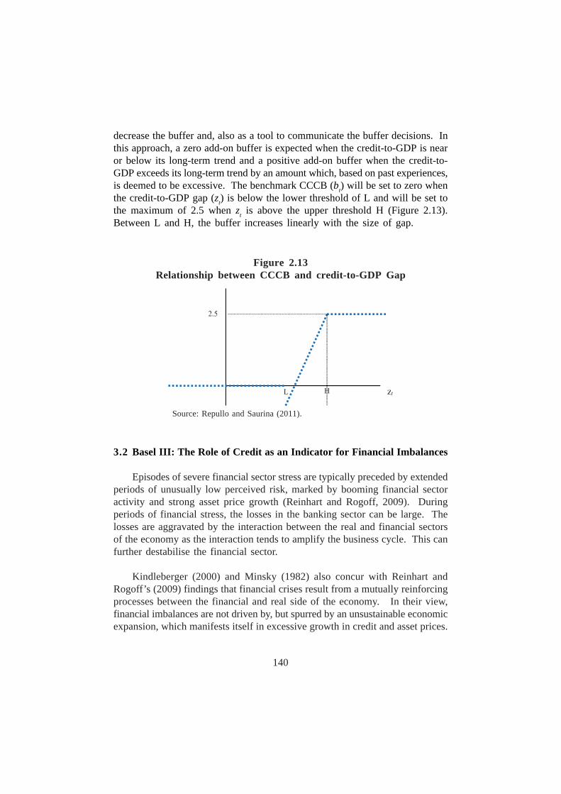
decrease the buffer and, also as a tool to communicate the buffer decisions. Inthis approach, a zero add-on buffer is expected when the credit-to-GDP is nearor below its long-term trend and a positive add-on buffer when the credit-to-GDP exceeds its long-term trend by an amount which, based on past experiences,is deemed to be excessive. The benchmark CCCB (bt) will be set to zero whenthe credit-to-GDP gap (zt) is below the lower threshold of L and will be set tothe maximum of 2.5 when zt is above the upper threshold H (Figure 2.13).Between L and H, the buffer increases linearly with the size of gap.

3.2 Basel III: The Role of Credit as an Indicator for Financial Imbalances

Episodes of severe financial sector stress are typically preceded by extendedperiods of unusually low perceived risk, marked by booming financial sectoractivity and strong asset price growth (Reinhart and Rogoff, 2009). Duringperiods of financial stress, the losses in the banking sector can be large. Thelosses are aggravated by the interaction between the real and financial sectorsof the economy as the interaction tends to amplify the business cycle. This canfurther destabilise the financial sector.

Kindleberger (2000) and Minsky (1982) also concur with Reinhart andRogoff’s (2009) findings that financial crises result from a mutually reinforcingprocesses between the financial and real side of the economy. In their view,financial imbalances are not driven by, but spurred by an unsustainable economicexpansion, which manifests itself in excessive growth in credit and asset prices.

Figure 2.13Relationship between CCCB and credit-to-GDP Gap

Source: Repullo and Saurina (2011).

141

When the economy expands, cash flows, incomes, asset prices and risk appetiteincrease in tandem with weakened funding constraints. This, further facilitatesrisk-taking activities. During this period, the financial system which has notbuild up sufficient capital and liquidity buffers to safeguard against the emergingrisks, may eventually cause a downturn in the economy. Therefore, the unwindingof the financial imbalances can potentially lead to a crisis, characterised by lossesand credit crunch in the financial sector. The close link between the real andfinancial sector provides justification for safeguarding the banks from financialpro-cyclicality and for banks to build-up capital in periods when there is excessivecredit growth.

While studies (Reinhart and Rogoff, 2009; Kindleberger, 2000 and Minsky,1982) show that credit is an important indicator for financial imbalances, others(Repullo and Saurina, 2011; Edger and Meisenzahl, 2011) argue that the credit-to-GDP is an unsuitable guide for the buffer because it does not meet the buffer’sobjectives. In particular, the credit-to-GDP gap guide may trigger pro-cyclicalchanges in the buffer. Repullo and Saurina (2011) show that the correlationbetween the credit-to-GDP gap and GDP growth is generally negative, whichmeans that the credit-to-GDP gap tends to signal a reduction of capitalrequirements when the GDP growth is high and an increase of capitalrequirements when the GDP is low. Consequently, the credit-to-GDP gap guideexacerbates the fluctuations in GDP. However, their analysis and findings focuseson advanced countries such as France, Germany, Italy, Japan, Spain and theUnited States7.

In addition to the pro-cyclicality argument, Edger and Meisenzahl (2011)argue that the credit-to-GDP gap measure is unreliable in real time since it issubjected to significant data revision. As such, it provides a poor foundation forpolicymaking as there is a tendency for the measure of the gap to give a falsesignal. For example, signalling excessive credit conditions which later may notappear to be so, when a longer time series of data is used. The false signalcan result in an increase in CCCB which in turn results in capital shortfalls inthe banking sector. Edger and Meisenzahl (2011) investigate and find instancesof which the credit-to-GDP gap produces a false positive, and in such episodes,the impact on loan volumes can be significant.

________________7. But the negative correlation is also found by Drehmann et al. (2012) for a panel of 53

countries. For Malaysia, the correlation between credit-to-GDP gap and seasonally adjustedGDP is negative. See section 5.3 for details.

142

From a practical perspective, there are issues with the measurementapproach for the credit-to-GDP gap. Critics highlighted that this measure issusceptible to the length of the time series and structural breaks in the data. Inthis regard, Geršl and Seidler (2011) point out that the Hodrick-Prescott (HP)filter technique which is recommended in Basel III, is a statistical filter whichdoes not take into account the economic fundamentals which affect the equilibriumof stock of loans. In this sense, the statistical approach does not rigorouslyestablish the relationship between the credit-to-GDP and the economicdevelopment of a country. An alternative method which estimates the equilibriumof loan levels in relation to the economy’s fundamentals may show that countriesat different stages of development will have different levels of loan equilibrium.While the HP filter approach is simple to adopt in calculating excessive credit,Geršl and Seidler (2011) suggest that the better approach would be the onewhich reflects the evolution of a country’s economic fundamentals. They alsoargued that a broader set of indicators and methods should be employed todetermine a country’s position in the credit cycle. Chen and Christensen (2010)in their study highlights the need to base the buffer decision on a broader rangeof indicators and to cross check these indicators with the credit-to-GDP gapguide. The reason is that they find that, in the case of Canada, an increase incredit-to-GDP ratio in late 2006, pre-GFC, was in line with the economic activity.This implies that the gaps do not signal excessive credit. However, the otherindicators such as house prices and equity prices were already steadily increasing,signalling a build-up in imbalances in the asset markets.

While the main arguments against the use of credit-to-GDP gap as a guidefor CCCB decisions are valid, Drehmann and Tsatsaronis (2014) point out thatthe critics have misinterpreted the objectives of the role of credit-to-GDP as abuffer guide. They argue that the CCCB framework provides the authoritieswith an instrument to base their decisions on, but not as an instrument to managethe credit cycle. Based on this viewpoint, the usefulness of the credit-to-GDPmust be judged exclusively on whether it provides policymakers with reliablesignals on when to raise the buffer. After reviewing the evidence, they foundthat the credit-to-GDP gap is on average (across many countries includingemerging economies and for several decades) the best single indicator.Furthermore, there are caveats in the Basel III framework with respect to themechanical usage of the credit-to-GDP gap. In particular, the Basel Committeeacknowledged that the gap may not be a good indicator of stress in downturnsand proposed to authorities to use judgement in making decisions to release thebuffer. This is a central feature of the CCCB framework which combines rulesand discretion.

143

Nevertheless, Drehmann et al. (2011) point out that the choice of the anchorvariable should meet four criteria namely: (i) It is able provide signals of goodand bad times; (ii) It should ensure that the size of the buffer build-up in goodtimes is sufficient to absorb subsequent losses when they materialise; (iii) Itshould be robust to regulatory arbitrage. The implementation of the guide isdifficult to be manipulated by individual institutions as well as being applicableto banking organisations that operate across borders and; (iv) It should betransparent and cost-effective.8

4. Methodology and Data

4.1 Choosing the Anchor Variable

The Basel Committee9 recommends the credit-to-GDP ratio as the anchorvariable in determining the countercyclical capital buffer but this has be disputedby Repullo and Saurina10 (2011) and Edger and Meisenzahl11 (2011). While theBasel Committee recommends the use of the credit-to GDP as an anchor forbuffer decisions, there are also a number of other research papers on the subjectthat recognises that the usefulness of other macro indicators12. This is becausethe credit-to-GDP ratio may not always be able to fully capture the informationon the financial cycles. There are several other indicators suggested in theliterature that could indicate a build-up of system-wide risk, such as house priceand equity price indices. Therefore, the paper analyses other macro variableswhich are related to the real economic and financial activities. The behaviourof these variables is assessed during the episodes of financial stress. Themacroeconomic variables examined are:

(i) Output gap, an indicator of the business cycle. The business and the financialcycles, although is closely linked, may not synchronise. However, in most

________________8. However, the Basel Committee allows the use of discretion by authorities. But, buffer

decisions must be communicated clearly to the public.

9. However, the Basel Committee recognises the fact that the credit-to-GDP gap may notalways work in all jurisdictions at all times. Nonetheless, for evolving the CCCB framework,it is expected that the national authorities would be transparent.

10. Repullo and Saurina (2011) argue that credit usually lags the business cycle. During periodsof downturns, the credit-to-GDP ratio continues to be high due to greater credit demandby households and firms which need credit o finance inventory accumulation.

11. Edge and Meisenzahl (2011) as well as Buncic and Melecky (2013) point out that thecredit-to-GDP gap is not necessarily an equilibrium notion of credit for the economy. Theydoubt that the credit gap can correctly identify periods of “excessive” credit growth.

12. See Chen and Christensen (2010) and Reserve Bank of India (2013).

144

cases, the spill overs of an overheating economy are evidenced in the assetmarkets and rapid credit growth;

(ii) Credit-to-GDP gap and credit growth. The credit-to-GDP gap benchmarkscredit growth with the overall economic activity and assess if credit isgrowing too fast compared with GDP; and

(iii) Asset prices. In general, property prices tend to show excessive increasesprior to a financial crisis and sharp declines during periods of financial stress(Drehmann et al., 2011). This paper examines equity and property pricegaps. The deviations from their long-term trends namely, the equity andproperty price gaps have proven useful in predicting banking crises (Borioand Drehmann, 2009).

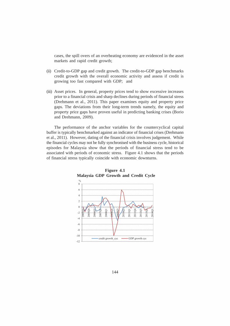
The performance of the anchor variables for the countercyclical capitalbuffer is typically benchmarked against an indicator of financial crises (Drehmannet al., 2011). However, dating of the financial crisis involves judgement. Whilethe financial cycles may not be fully synchronised with the business cycle, historicalepisodes for Malaysia show that the periods of financial stress tend to beassociated with periods of economic stress. Figure 4.1 shows that the periodsof financial stress typically coincide with economic downturns.

Figure 4.1 Malaysia GDP Growth and Credit Cycle

145

4.2 Estimating the Gaps of Macro Variables Using the Hodrick-Prescott(HP) Filter

This paper derives the gaps for all the macro variables, namely the output,the credit-to-GDP, the house price and equity prices by using the two-sidedHodrick-Prescott (HP) filter. Although, the one-sided Hodrick-Prescott filter isrecommended by the Basel Committee to address the bias end point problem13,the results from the two-sided HP filter tend to produce a more precise estimateof the trend as it uses all available information (Gerdrup, Bakke Kvinlog andSchaanning, 2013). The paper analyses the performance of the gap estimatesfrom the one-sided and two-sided HP filter and finds that the two-sided filterproduces gap estimates that are more indicative of the financial stress periods14.Furthermore, to derive a reasonable trend using the one-sided HP filter wouldrequire a long time series (Reserve Bank of India, 2013). Given the limitationsof data availability, in particular, the quarterly property prices (sample startsfrom 1Q 1999), using the one-sided filter may not feasible. Furthermore, thetwo-sided filter is found to provide a more precise estimate of the trend (Gerdrupet al., 2013).

Ravn and Uhlig (2002) show that for cycles with longer durations, such asthe credit cycle, a higher λ value is considered appropriate as the smoothingparameter for the HP filter. Their findings were adopted and used asrecommendation by the Basel Committee15, where long-term trends in creditare extracted using the smoothing parameter of λ = 400,000. Drehmann et al.(2011) also set λ at 400,000 as crises occur on average in 20-25 years in theirsample. However, the paper sets the smoothing parameter λ to 1600, aconventional value for quarterly data since the average length of Malaysiafinancial cycles is almost similar to its business cycle (Figure 4.1). The decisionis also based on the ad-hoc tests conducted on various values of lambda. Thestudy finds that λ = 400,000 produces a higher noise-to-signal ratio comparedto λ = 1600 (see Table 5.3).

________________13. The end point bias from the two-sided HP filter results from unavailability of observed

values towards the end of the sample. When the future observations of the series areunavailable, the last point of the series will have an exaggerated impact on the trend.Another drawback of the HP filter is in its inability to account for structural breaks(Sarmento, 1998). To address the end-point bias, literature suggests an extension of thesample period (Mohr, 2005).

14. See Section 5.5.15. Ibid.

146

4.3 Identification of an Appropriate Threshold Level

The lower and upper thresholds, L and H set for the benchmark variable(credit-to-GDP gap) determines the timing and the speed of adjustment for thecapital buffer add on. Based on historical banking crisis, the Basel Committeehas found the lower threshold of L=2 and upper threshold of H=10 to providea reasonable and robust specification. The Basel Committee recommends amaximum buffer add-on of 2.5% of risk weighted assets when the credit-to-GDP ratio exceeds its long-term trend by 10 percentage points or more. Whenthe credit-to-GDP gap is between 2 to 10 percentage points, the buffer add-onwill increase linearly between 0% to 2.5%.

While the thresholds for credit-to-GDP gaps are prescribed by the Committee,it can be calibrated to suit the domestic economic conditions. The calibrationis to ensure that the implementation of capital buffers does not stifle economicgrowth. Therefore, in this study, the Basel framework is tested and if required,suitable modifications to the thresholds will been made.

In this context, various thresholds for the benchmark macro variables aretested and the appropriate level of threshold is identified based on two approaches:(i) Sarel’s (1996) approach or; (ii) Kaminsky and Reinhart’s (1999) approach.

In Sarel’s (1996) approach, a regression with different thresholds is testediteratively. The threshold is determined based on the explanatory power ofequation (1) and the significance of the coefficient.

nplt = α0 + α1bigapt-i + α2tht-i * (bigapt-i) + ysat-i + nplt-i (1)i = 1,2,,3 ... . .,8 ; t = 1,2 ... . .,92

where npl is non-performing loans of banking system (based on 3 monthsclassification), ysa is seasonally adjusted gross domestic product (GDP) growth,the benchmark indicator gap which includes credit-to-GDP, house price, equityprice and output gaps, th value is value which the threshold is set.

th is a dummy, th = 1 if benchmark indicator gap > threshold value, and,th = 0 otherwise.

The second approach is a “signalling” approach which evaluates discretethresholds by measuring the noise-to-signal ratios. The threshold for the

147

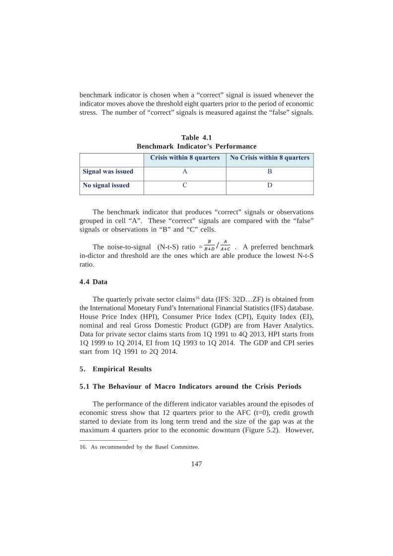
benchmark indicator is chosen when a “correct” signal is issued whenever theindicator moves above the threshold eight quarters prior to the period of economicstress. The number of “correct” signals is measured against the “false” signals.

The benchmark indicator that produces “correct” signals or observationsgrouped in cell “A”. These “correct” signals are compared with the “false”signals or observations in “B” and “C” cells.

The noise-to-signal (N-t-S) ratio = . A preferred benchmarkin-dictor and threshold are the ones which are able produce the lowest N-t-Sratio.

4.4 Data

The quarterly private sector claims16 data (IFS: 32D…ZF) is obtained fromthe International Monetary Fund’s International Financial Statistics (IFS) database.House Price Index (HPI), Consumer Price Index (CPI), Equity Index (EI),nominal and real Gross Domestic Product (GDP) are from Haver Analytics.Data for private sector claims starts from 1Q 1991 to 4Q 2013, HPI starts from1Q 1999 to 1Q 2014, EI from 1Q 1993 to 1Q 2014. The GDP and CPI seriesstart from 1Q 1991 to 2Q 2014.

5. Empirical Results

5.1 The Behaviour of Macro Indicators around the Crisis Periods

The performance of the different indicator variables around the episodes ofeconomic stress show that 12 quarters prior to the AFC (t=0), credit growthstarted to deviate from its long term trend and the size of the gap was at themaximum 4 quarters prior to the economic downturn (Figure 5.2). However,

Table 4.1Benchmark Indicator’s Performance

________________16. As recommended by the Basel Committee.

/

148

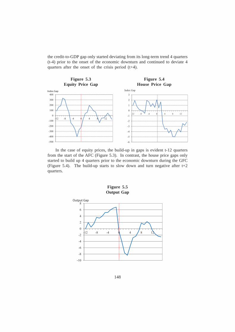
the credit-to-GDP gap only started deviating from its long-term trend 4 quarters(t-4) prior to the onset of the economic downturn and continued to deviate 4quarters after the onset of the crisis period (t+4).

In the case of equity prices, the build-up in gaps is evident t-12 quartersfrom the start of the AFC (Figure 5.3). In contrast, the house price gaps onlystarted to build up 4 quarters prior to the economic downturn during the GFC(Figure 5.4). The build-up starts to slow down and turn negative after t+2quarters.

Figure 5.3Equity Price Gap

Figure 5.4House Price Gap

Figure 5.5Output Gap

149

The output gap show signs of a build-up as early as 12 quarters leading upto AFC. The output gap peaked at around 6%, one quarter prior to the economiccrisis and it turned negative at t=0.

5.2 Correlation between Indicator Variables and GDP

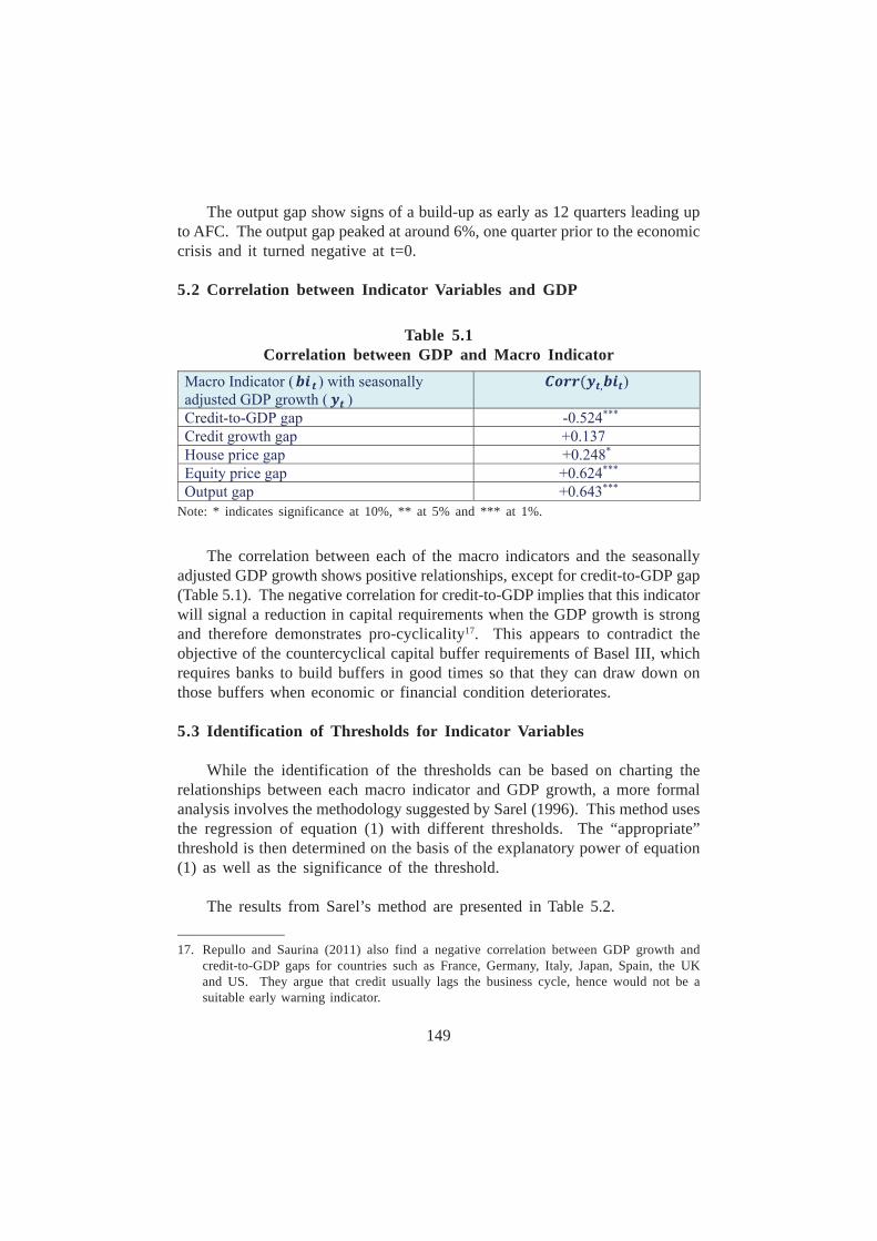
Table 5.1Correlation between GDP and Macro Indicator

Note: * indicates significance at 10%, ** at 5% and *** at 1%.

The correlation between each of the macro indicators and the seasonallyadjusted GDP growth shows positive relationships, except for credit-to-GDP gap(Table 5.1). The negative correlation for credit-to-GDP implies that this indicatorwill signal a reduction in capital requirements when the GDP growth is strongand therefore demonstrates pro-cyclicality17. This appears to contradict theobjective of the countercyclical capital buffer requirements of Basel III, whichrequires banks to build buffers in good times so that they can draw down onthose buffers when economic or financial condition deteriorates.

5.3 Identification of Thresholds for Indicator Variables

While the identification of the thresholds can be based on charting therelationships between each macro indicator and GDP growth, a more formalanalysis involves the methodology suggested by Sarel (1996). This method usesthe regression of equation (1) with different thresholds. The “appropriate”threshold is then determined on the basis of the explanatory power of equation(1) as well as the significance of the threshold.

The results from Sarel’s method are presented in Table 5.2.________________17. Repullo and Saurina (2011) also find a negative correlation between GDP growth and

credit-to-GDP gaps for countries such as France, Germany, Italy, Japan, Spain, the UKand US. They argue that credit usually lags the business cycle, hence would not be asuitable early warning indicator.

150

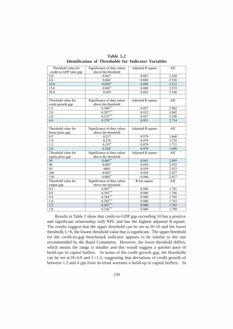
Table 5.2Identification of Thresholds for Indicator Variables

Results in Table 2 show that credit-to-GDP gap exceeding 10 has a positiveand significant relationship with NPL and has the highest adjusted R-square.The results suggest that the upper threshold can be set as H=10 and the lowerthreshold, L=6, the lowest threshold value that is significant. The upper thresholdfor the credit-to-gap benchmark indicator appears to be similar to the onerecommended by the Basel Committee. However, the lower threshold differs,which means the range is smaller and this would suggest a quicker pace ofbuild-ups in capital buffers. In terms of the credit growth gap, the thresholdscan be set at H=4.0 and L=1.5, suggesting that deviations of credit growth ofbetween 1.5 and 4 ppt from its trend warrants a build-up in capital buffers. In

151

the case of equity price gaps and output gaps, the upper and lower thresholdscan be set at H=130 and L=50 and H=1.5 and L=0.5 respectively.

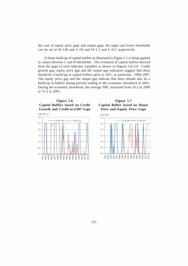
A linear build-up of capital buffers as illustrated in Figure 2.1 is being appliedto values between L and H thresholds. The evolution of capital buffers derivedfrom the gaps of each indicator variables is shown in Figures 5.6-5.9. Creditgrowth gap, equity price gap and the output gap indicators suggest that thereshould be a build-up in capital buffers prior to AFC, in particular, 1996-1997.The equity price gap and the output gap indicate that there should also be abuild-up in buffers during periods leading to the economic slowdown in 2001.During the economic slowdown, the average NPL increased from 10.2 in 2000to 11.3 in 2001.

Figure 5.6Capital Buffers based on CreditGrowth and Credit-to-GDP Gaps

Figure 5.7Capital Buffer based on House

Price and Equity Price Gaps

152

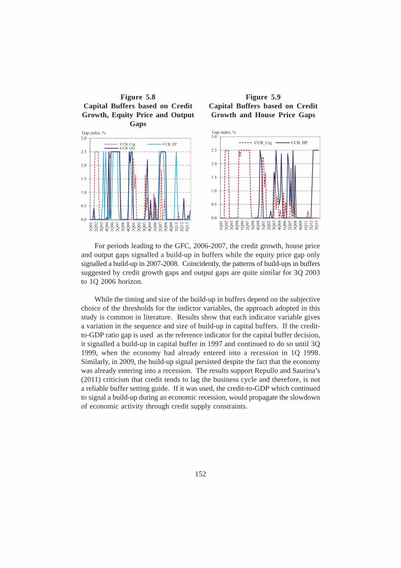
Figure 5.8Capital Buffers based on CreditGrowth, Equity Price and Output

Gaps

Figure 5.9Capital Buffers based on CreditGrowth and House Price Gaps

For periods leading to the GFC, 2006-2007, the credit growth, house priceand output gaps signalled a build-up in buffers while the equity price gap onlysignalled a build-up in 2007-2008. Coincidently, the patterns of build-ups in bufferssuggested by credit growth gaps and output gaps are quite similar for 3Q 2003to 1Q 2006 horizon.

While the timing and size of the build-up in buffers depend on the subjectivechoice of the thresholds for the indictor variables, the approach adopted in thisstudy is common in literature. Results show that each indicator variable givesa variation in the sequence and size of build-up in capital buffers. If the credit-to-GDP ratio gap is used as the reference indicator for the capital buffer decision,it signalled a build-up in capital buffer in 1997 and continued to do so until 3Q1999, when the economy had already entered into a recession in 1Q 1998.Similarly, in 2009, the build-up signal persisted despite the fact that the economywas already entering into a recession. The results support Repullo and Saurina’s(2011) criticism that credit tends to lag the business cycle and therefore, is nota reliable buffer setting guide. If it was used, the credit-to-GDP which continuedto signal a build-up during an economic recession, would propagate the slowdownof economic activity through credit supply constraints.

153

5.4 Evaluation of Gaps and Thresholds based on the Noise-to-SignalApproach

Another approach in selecting appropriate thresholds is the “noise” and“signal” approach. The threshold is determined in such a way that the indicatorvariable is able to exhibit an excessive build-up and hence, crosses the thresholdeight quarters prior to a financial distress18. Three major economic events areused in the dating of the financial cycle, namely, the Asian Financial Crisis (AFC)1998/99, the Burst Tech Bubble 2000/01 and the Global Financial Crisis (GFC)2008/09. The dating process is based on Malaysia’s past episodes of economicdistress when financial distress was also evident.

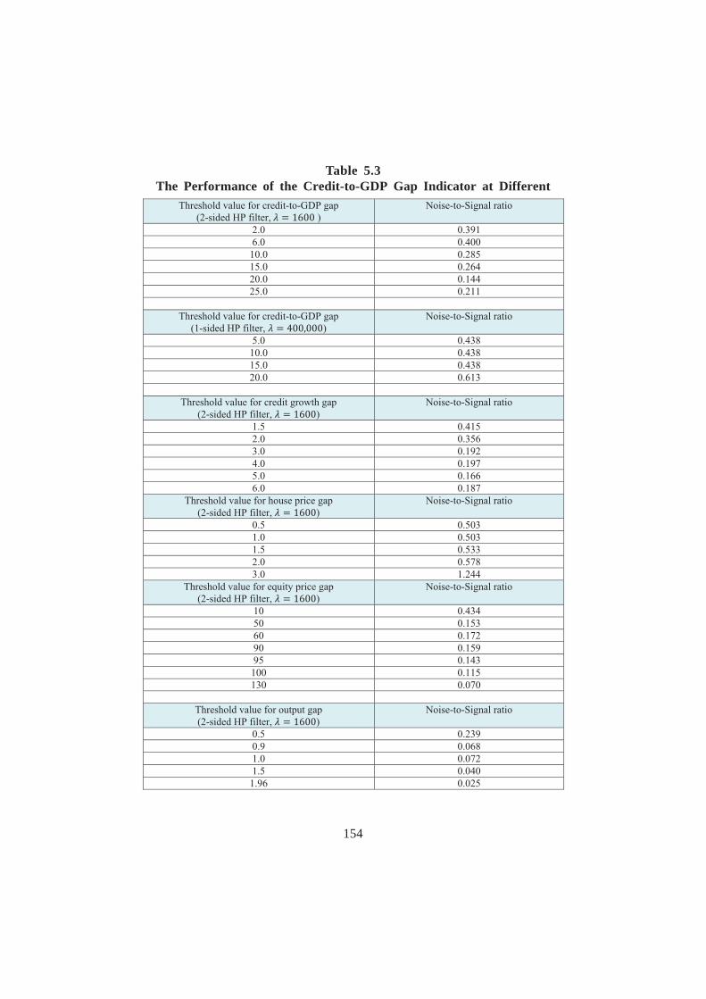
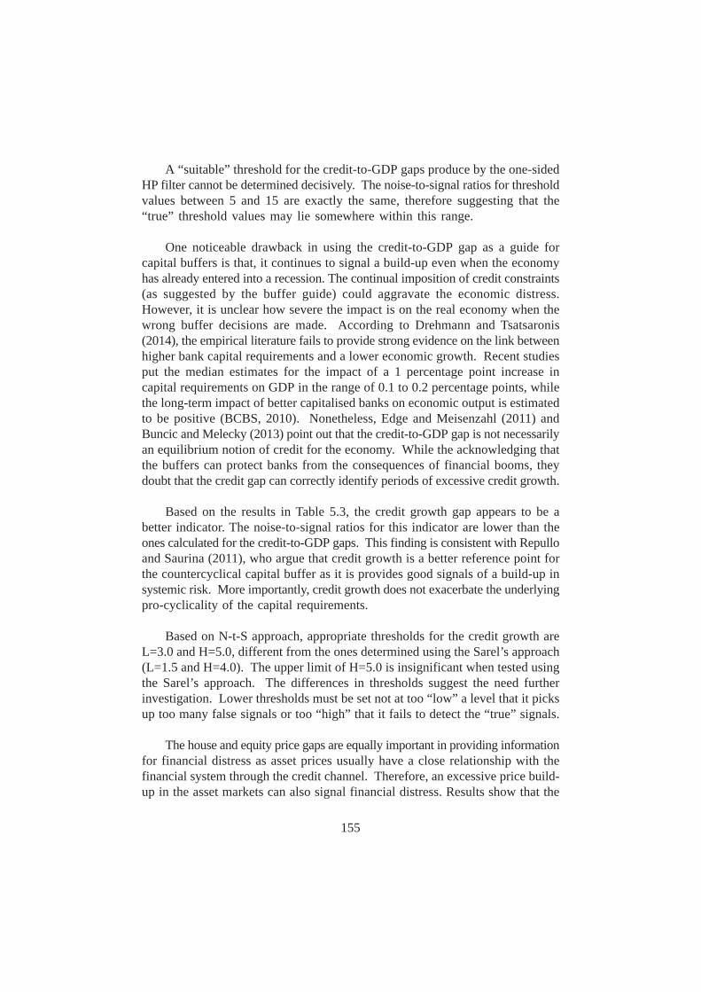
Since the Basel Committee recommends the use of the one-sided HP filterwith =400,000, the results of the credit-to-GDP gap derived from both the one-sided and two-sided HP filters with different thresholds are compared and shownin Table 5.3. From the results, the two-sided HP filter consistently produceslower noise-to-signal ratios at each of the thresholds compared to the one-sidedHP filter. From the results, appropriate thresholds for the credit-to-GDP gapderived from the two-sided HP filter L=2 and H=20, instead of L=6 and H=10as suggested from Sarel’s approach. A wider range for capital build-ups (L=2,H=20) suggests that the pace of the build-up of capital buffers will be slightlyslower during periods of excessive credit-to-GDP gaps.

________________18. For details of the methodology, see Section 4.3.

154

Table 5.3The Performance of the Credit-to-GDP Gap Indicator at Different

155

A “suitable” threshold for the credit-to-GDP gaps produce by the one-sidedHP filter cannot be determined decisively. The noise-to-signal ratios for thresholdvalues between 5 and 15 are exactly the same, therefore suggesting that the“true” threshold values may lie somewhere within this range.

One noticeable drawback in using the credit-to-GDP gap as a guide forcapital buffers is that, it continues to signal a build-up even when the economyhas already entered into a recession. The continual imposition of credit constraints(as suggested by the buffer guide) could aggravate the economic distress.However, it is unclear how severe the impact is on the real economy when thewrong buffer decisions are made. According to Drehmann and Tsatsaronis(2014), the empirical literature fails to provide strong evidence on the link betweenhigher bank capital requirements and a lower economic growth. Recent studiesput the median estimates for the impact of a 1 percentage point increase incapital requirements on GDP in the range of 0.1 to 0.2 percentage points, whilethe long-term impact of better capitalised banks on economic output is estimatedto be positive (BCBS, 2010). Nonetheless, Edge and Meisenzahl (2011) andBuncic and Melecky (2013) point out that the credit-to-GDP gap is not necessarilyan equilibrium notion of credit for the economy. While the acknowledging thatthe buffers can protect banks from the consequences of financial booms, theydoubt that the credit gap can correctly identify periods of excessive credit growth.

Based on the results in Table 5.3, the credit growth gap appears to be abetter indicator. The noise-to-signal ratios for this indicator are lower than theones calculated for the credit-to-GDP gaps. This finding is consistent with Repulloand Saurina (2011), who argue that credit growth is a better reference point forthe countercyclical capital buffer as it is provides good signals of a build-up insystemic risk. More importantly, credit growth does not exacerbate the underlyingpro-cyclicality of the capital requirements.

Based on N-t-S approach, appropriate thresholds for the credit growth areL=3.0 and H=5.0, different from the ones determined using the Sarel’s approach(L=1.5 and H=4.0). The upper limit of H=5.0 is insignificant when tested usingthe Sarel’s approach. The differences in thresholds suggest the need furtherinvestigation. Lower thresholds must be set not at too “low” a level that it picksup too many false signals or too “high” that it fails to detect the “true” signals.

The house and equity price gaps are equally important in providing informationfor financial distress as asset prices usually have a close relationship with thefinancial system through the credit channel. Therefore, an excessive price build-up in the asset markets can also signal financial distress. Results show that the

156

noise-to-signal ratios for equity price gaps perform better than the house pricegaps. The thresholds for both indicators are found to be at L=50, H=130 and;L=0.5, H=1.5 respectively. The appropriate lower and upper thresholds forequity price are similar to the ones identified from Sarel’s approach. However,the range for the house price is narrower compared with the Sarel’s approach.The narrower range suggests that the pace of the build-up in capital would needto be much quicker. These indicators do not only provide information on thedevelopments of the asset markets at different business cycles, but they arealso quicker in signally a release in buffers when the economic condition worsens.For example, during the economic downturns in 1998, 2001 and 2009, the gapsfor these indicators, in particular the equity price indicator turned negative,therefore signalling a stop in the build-up of buffers. This is not evident fromthe credit-to-GDP gap indicator.

The output gap appears to contain important information on the build-up offinancial risks. Given that credit supports consumption and investment, excessivegrowth in private sector loans can over stimulate aggregate demand beyondpotential output. A build-up in output gaps signals an overheating of the economywith potentially rising price pressures and current account imbalances. Therefore,the link between the financial and the real sectors through the credit channelsuggests that an overheating economy tend to be associated with a strong creditdemand and a weak economy with a low credit demand19. From the findings,the output gap indicator registers the lowest noise-to-signal ratios among allindicators. The upper and lower threshold is found to be at L=0.9 and H=1.96,slightly different from the thresholds identified from Sarel’s approach (L=0.5and H=2.0).

6. Conclusion

The financial crisis in 2008 has amplified the weaknesses in the globalregulatory framework and in the banks’ risk management practices. Thisweakness propagated a vicious cycle where problems in the financial systemspill over into the real economy which, in turn worsens the banking sector throughthe feedback loop. Consequently, the new Basel III framework which includesthe introduction of countercyclical capital buffers (CCCB), aimed at increasingthe resilience of the banking system and its capacity to absorb financial andeconomic shocks during crises. In particular, the CCCB is expected to mitigatethe tendency of bank capital regulation which amplifies the pro-cyclicality inlending conditions. As such, buffers are expected to increase during periods of________________19. VAR Granger Causality test shows that the output gap granger causes NPLs.

157

excessive credit growth which tends to be associated with increasing financialrisks. They will be released during financial stress in order to help banks absorblosses.

The paper assesses the conceptual and practical criticisms of the credit-to-GDP gap as the recommended anchor for the implementation of thecountercyclical capital buffers under Basel III. The credit-to-GDP indicatorhas two limitations: (i) While both nominal credit and GDP are falling, the ratioactually increases because the GDP (denominator) falls more rapidly - whichwill result in misleading buffer guides, and (ii) The credit-to-GDP ratio does notallow for the possibility of differing credit and output trends, which is importantif countries are undergoing a process of financial deepening (Elekdag and Wu,2011). The findings in the paper show that credit-to-GDP may trigger pro-cyclical changes in the buffers, in particular, it signals a continual build-up incapital buffers during periods of recessions. This concurs with the first limitationhighlighted by Elekdag and Wu (2011). Other critics such as Buncic and Melecky(2013) argue that the one-sided filtered credit-to-GDP fails to adequately capturethe shifts in equilibrium credit in line with the changing phases of developmentof a country.

The practical implementation of the one-sided filter with the recommendedsmoothing parameter of λ = 400,000, is also subjected to measurement issues.The length of the underlying credit-to-GDP cycle which is reflected in the choiceof λ is subjective. Furthermore, the HP filter is a statistical approach that doesnot treat structural breaks in the data series adequately20. The HP filter accountfor varying levels of optimal of credit needed for countries at different stagesof development. This statistical approach does not allow calibration of equilibriumcredit to account for the development goals set by the policy makers (Buncicand Melecky, 2013).

The empirical findings show that thresholds identified for the credit-to-GDPindicator differ slightly from the thresholds suggested by the Basel Committee.However, as highlighted in the results, the signal for a build-up in capital continueseven after the economy enters a recession. The empirical evidence in the papershows that other indicators such as credit growth and asset price indicators tendto perform better in terms of giving “correct” signals prior to an economic distress.All the other indicators except for the house price indicator tend to producelower noise-to-signal ratios. This suggests that composite indicators may provide

________________20. Drehmann and Tsatsaronis (2014) found from their simulation that it takes at least 10 years

for impact of the structural break on the credit-to-GDP to normalise.

158

a more broad-based view of the financial conditions rather than a single indicatorat any given point in time21. Including the output gap expands the understandingof the conditions of the financial and real sectors, which are mutually dependent.Lowe (2002) as well as Behn et al. (2013) found that combinations of the creditgap and a similarly calculated asset price gap produce a more precise signal.

The findings in this paper highlight the challenges in using a single indicatorand an identified threshold as the countercyclical capital buffer guide across allcyclical phases. Some indicators that perform better during certain periods maycease to be useful after a certain phase of economic development22. Sincethere is no perfect model that can deliver the decision for an effective rule-based countercyclical instrument, the policymakers are expected to use judgmentas well as quantitative analysis within the parameters of the framework. Thisis supported by the empirical findings of the paper which requires some judgmentin the interpretation of gaps and the thresholds and in turn, this would have animplication on the timing, the size and pace of build ups in capital buffers.

In addition, Malaysia is still a developing economy and therefore, theinteraction between the real and financial sectors of the economy is changingover time. The strict application of the credit gap rule may impede financialdeepening. As highlighted by the World Bank (2010) and the Reserve Bank ofIndia (2013), economies that go through the process of financial developmentcan experience prolonged periods of credit growth. Therefore, limiting creditgrowth could potentially affect financial deepening and slow the process ofcatching up with financially more advanced economies.

In summary, there is still no clear consensus on the best indicator to usefor countercyclical capital buffer decisions. The lack of convincing evidence inusing the credit-to-GDP gap as a sole indicator for countercyclical capital bufferdecisions is highlighted in the findings of this paper. As such, the paper exploresthe information contained in a range of macro indicators in order to obtain amore balanced view about the build-up of financial risks in the economy. Whileempirical analysis does not provide a clear guidance for the countercyclical bufferdecisions, it provides useful references for policy debates. The analysis suggests

________________21. While Drehmann and Tsatsaronis (2014) found the credit-to-GDP gap to be on average the

best single indicator even for emerging market economies, they cannot discount the fact thatcomposite indicators may perform better at any particular point in time.

22. Future work may be required to investigate the relationship between the macro indicatorsand the sources of financial vulnerability and the changing relationship during the differentphases of economic development.

159

that the practical application of model-based results needs to be balanced withsome elements of judgement and discretion. At this point, it may be prematureto conclude from the findings that any rule-based decision can be formulated forMalaysia and would be sufficiently robust across time. The policymaker wouldstill need to exercise judgement in assessing whether the credit-to-GDP gap orany macro indicator that crosses a pre-determined threshold is unsustainableand a source of financial vulnerability to the economy.

160

References

Bank Negara Malaysia, (2001), Financial Sector Masterplan (FSMP).

Bank Negara Malaysia, (2011), Financial Sector Blueprint 2011-2020.

Basel Committee on Banking Supervision, (2010), Guidance for NationalAuthorities Operating the Countercyclical Capital Buffer, December.

Borio, C. and M. Drehmann, (2009), “Assessing the Risk of Banking Crises –Revisited,” BIS Quarterly Review, March, pp. 29–46.

Borio, C. and P. Lowe, (2002), “Assessing the Risk of Banking Crises,” BISQuarterly Review, December, pp. 43–54.

Buncic, D. and M. Melecky, (2013), “Equilibrium Credit: The Reference Pointfor Macroprudential Supervision,” Policy Research Working Paper, No.6358, World Bank, February.

Chen, X. D. and I. Christensen, (2010), “The Countercyclical Bank Capital Buffer:Insights for Canada,” Financial System Review, December, pp. 29-34.

Drehmann, M. and K. Tsatsaronis, (2014), “The Credit-to-GDP Gap andCountercyclical Capital Buffers: Questions and Answers,” BIS QuarterlyReview, March, pp. 55-73.

Drehmann, M., (2013), “Total Credit as an Early Warning Indicator for SystemicBanking Crises,” BIS Quarterly Review, June, pp. 41–5.

Drehmann, M.; C. Borio and K. Tsatsaronis, ( 2011), “Anchoring CountercyclicalCapital Buffers: The Role of Credit Aggregates,” BIS Working Papers,No. 355.

Drehmann, M.; C. Borio and K. Tsatsaronis, (2012), Characterising the FinancialCycle: Don’t Lose Sight of the Medium Term!” BIS Working Papers,No. 380.

Drehmann, M. and M. Juselius, (2012), “Do Debt Service Costs AffectMacroeconomic and Financial Stability?” BIS Quarterly Review, September,pp. 21–34.

161

Edge, R. and R. Meisenzahl, (2011), “The Unreliability of Credit-To-GDP RatioGaps in Real-Time: Implications for Countercyclical Capital Buffers,”International Journal of Central Banking, December, pp. 261–98.

Elekdag, S. and Y. Wu, (2011), “Rapid Credit Growth: Boon or Boom-Bust?”IMF Working Paper, WP/11/241, International Monetary Fund.

Gerdrup, K.; A. Kvinlog and E. Schaanning, (2013), “Key Indicators for aCountercyclical Capital Buffer in Norway – Trends and Uncertainty,” StaffMemo, No. 13/2013, Financial Stability, Central Bank of Norway (NorgesBank).

Geršl, A. and J. Seidler, (2012), “Excessive Credit Growth and CountercyclicalCapital Buffers in Basel III: An Empirical Evidence from Central and EastEuropean Countries,” Economic Studies and Analyses, No. 6(2).

International Monetary Fund, (2014), “Malaysia: Financial Sector AssessmentProgram Stress Testing The Malaysia and Labuan IBFC Banking Sector- Technical Note,” IMF Country Report, No. 14/97.

Jiménez, G. and J. Saurina, (2006), “Credit Cycles, Credit Risk and PrudentialRegulation,” International Journal of Central Banking, No. 2, pp. 65-98.

Kaminsky, G. L. and C. M. Reinhart, (1999), “The Twin Crises: The Causesof Banking and Balance of Payments Problems,” The American EconomicReview, Vol. 89(3), pp. 473-500.

Kindleberger, C., (2000), Maniacs, Panics and Crashes, Cambridge UniversityPress, Cambridge.

Minsky, H., (982), Can “It” Happen Again? Essays on Instability and Finance,M. E. Sharpe, Armonk.

Mohr, M., (2005), “A Trend-cycle (-season) Filter,” ECB Working Paper Series,No. 499.

Morgan, P. J. and V. Pontines, (2013), “An Asian Perspective on GlobalFinancial Reforms,” ADBI Working Paper Series, No. 433, August, AsianDevelopment Bank Institute (ADBI).

162

Ravn, M. O. and H. Uhlig, (2002), “On Adjusting the Hodrick-Prescott Filterfor the Frequency of Observations,” Review of Economics and Statistics,Vol. 84(2), pp. 371-6.

Repullo, R. and J. Saurina, (2011), “The Countercyclical Capital Buffer of BaselIII: A Critical Assessment,” CEPR Discussion Paper, No. 8304, Centreof European Policy Research.

Reinhart, C.M. and K. S. Rogoff, (2009), “The Aftermath of Financial Crisis,”NBER Working Paper Series, W14656, The National Bureau of EconomicResearch, Cambridge.

Reserve Bank of India, (2013), Report of the Internal Working Group onImplementation of Countercyclical Capital Buffer, Draft, December.

Sarel, M., (1996), “Nonlinear Effects of Inflation on Growth,” IMF Staff Papers,Vol. 43, No. 1. International Monetary Fund.

Sarmento, L., (1998), “The Use of Cyclically Adjusted Balances at Banco DoPortugal,” Bank of Italy – Indicators of Structural Budget BalancesConference, pp. 273.

Saurina, J.; J. Gabriel; S. Ongena and J. Peydro, (2008), “Hazardous Times forMonetary Policy: What Do 23 Million Bank Loans Say About the Effectsof Monetary Policy on Credit Risk?” Discussion Paper, No. 75, Centerof Economic Research, Tilburg University.

Van Norden, S., (2011), “Discussion of the Unreliability of Credit-to-GDP RatioGaps in Real-time: Implications for Countercyclical Capital Buffers,”International Journal of Central Banking, December, pp. 300–3.