Chapter 3 Vector Spaces and Linear Transformationskilyos.ee.bilkent.edu.tr/~sezer/EEE501/Chapter3.pdf · Chapter 3 Vector Spaces and Linear Transformations 3.1 Vector Spaces Recall

Chapter 3

Vector Spaces and Linear

Transformations

3.1 Vector Spaces

Recall that a vector in the xy plane is a line segment directed from the origin to apoint in the plane as shown in Figure 3.1. Recall also that the sum of two vectors v1

and v2 is a vector obtained by the parallelogram rule. Also, for a real number c, cvis a vector whose magnitude is |c| times the magnitude of v and whose direction isthe same as the direction of v if c > 0, and opposite to the direction of v if c < 0.

A convenient way to represent a vector in the xy plane is to consider it as anordered pair of two real numbers as v = (α, β) where α and β are the componentsof v along the x and y axes. This representation allows us to define the sum of twovectors v1 = (α1, β1) and v2 = (α2, β2) in terms of their components as

v1 + v2 = (α1 + α2, β1 + β2)

and a scalar multiple of a vector v = (α, β) as

cv = (cα, cβ)

The representation of a vector in the xy plane by a pair also allows us to derivesome desirable properties of vector addition and scalar multiplication. For example,

v1 + v2 = (α1 + α2, β1 + β2) = (α2 + α1, β2 + β1) = v2 + v1

and

(c + d)v = ((c + d)α, (c + d)β) = (cα, cβ) + (dα, dβ) = cv + dv

Finally, such a representation is useful in expressing a given vector in terms ofsome special vectors. For example, defining i = (1, 0) and j = (0, 1) to be the unitvectors along the x and y axes, we have

v = (α, β) = α (1, 0) + β (0, 1) = α i + β j

The idea of representing a vector in a plane by an ordered pair can be generalizedto vectors in three dimensional xyz space, where we represent a vector v by a triple(α, β, γ), with α, β, and γ corresponding to the components of v along the x, y,and z axes. What about a quadruple (α, β, γ, δ)? Although we cannot visualize itas an arrow in a four dimensional space, we can still define the sum of two such

85

86 Vector Spaces and Linear Transformations

0

0

y

x

v1

v1+v

2

v1−v

2

v2

−v2

2v1

Figure 3.1: Representation of vectors in a plane

quadruples as well as a scalar multiple of a quadruple in terms of their components.This motivates the need for a more general and abstract definition of a vector.1

3.1.1 Definitions

A vector space X over a field F is a non-empty set, elements of which are calledvectors, together with two operations called addition and scalar multiplication

that have the following properties.Addition operation associates with any two vectors x,y ∈ X a unique vector

denoted x + y ∈ X, and satisfies the following conditions.

A1. x + y = y + x for all x,y ∈ X.

A2. x + (y + z) = (x + y) + z for all x,y, z ∈ X.

A3. There exists an element of X, denoted 0, such that x + 0 = x for all x ∈ X.0 is called the zero vector or the null vector.

A4. For any x ∈ X there is a vector −x ∈ X such that x + (−x) = 0.

Scalar multiplication operation associates with any vector x ∈ X and any scalarc ∈ F a unique vector denoted cx ∈ X, and satisfies the following conditions.

S1. (cd)x = c(dx) for all x ∈ X and c, d ∈ F.

S2. 1x = x for all x ∈ X, where 1 is the multiplicative identity of F.

S3. (c + d)x = cx + dx for all x ∈ X and c, d ∈ F.

S4. c(x + y) = cx + cy for all x,y ∈ X and c ∈ F.

If the field over which a vector space is defined is clear from the context, we omitthe phrase “over F” when referring to a vector space.

The following properties of a vector space follow directly from the definition.

1The reader may be accustomed to defining any directed line segment in the plane, such as anarrow directed from the tip of v1 to the tip of v1 + v2 in Figure 3.1, as a vector. However, thisis just a visual aid, and as far as the addition and scalar multiplication operations just defined areconcerned, that arrow is no different from v2. In this sense, v2 represents all arrows that have thesame orientation and the same length as v2, which form an equivalence class.

3.1 Vector Spaces 87

a) 0 is unique

b) −0 = 0

c) 0x = 0 for all x ∈ X

d) c0 = 0 for all c ∈ F

e) −x is unique for any x ∈ X

f) (−1)x = −x for any x ∈ X

To prove (a), assume that there are two different vectors 01 6= 02 satisfying con-dition A3. Then 02 + 01 = 02 (A3 with x = 02 and 0 = 01), and also 01 + 02 = 01

(A3 with x = 01 and 0 = 02). Then, by A1 we have 02 = 01, contradicting theassumption. Therefore, there can be no two distinct 0’s. Other properties can beproved similarly, and are left to the reader as an exercise.

Example 3.1

Consider the set of all ordered n-tuples2 of the form

x = (x1, x2, . . . , xn)

where x1, x2, . . . , xn ∈ F. Defining addition and scalar multiplication operations element-by-element as

(x1, x2, . . . , xn) + (y1, y2, . . . , yn) = (x1 + y1, x2 + y2, . . . , xn + yn)

c (x1, x2, . . . , xn) = (cx1, cx2, . . . , cxn)

and letting

0 = (0, 0, . . . , 0)

−(x1, x2, . . . , xn) = (−x1,−x2, . . . ,−xn)

all the properties of the vector addition and scalar multiplication are satisfied. Thus theset of all n-tuples of F is a vector space over F, called the n-space and denoted F

n. Areal n-tuple is (x1, x2, . . . , xn) is an obvious generalization of the familiar concept of avector in the plane.

In particular, R1, R

2 and R3 can be identified with the real line, the xy plane and

the xyz space, respectively.3

Example 3.2

The set of m×n matrices, Fm×n, together with the matrix addition and scalar multipli-

cation operations defined in Section 1.2 is a vector space.4

In particular, F1×n and F

n×1 are vector spaces. This is why we call a row matrixalso a row vector, and a column matrix a column vector. In fact, both F

1×n and Fn×1

can be identified with Fn in Example 3.1. In other words, an n-tuple can be viewed as an

2From now on, we will distinguish an ordered set from an unordered set by enclosing its elementswith parantheses rather than curly brackets

3Note that the set of real numbers is both a field and also a vector space. We distinguish the twoby denoting the real field by R and the vector space of real numbers by R

1.4The reader might ask: “When we multiply two n × n matrices, are we multiplying two vectors

in Fm×n? Can we similarly multiply two vectors in R

n”? The answer is that when we multiplytwo matrices, we do not view them as vectors, but as something else that we will consider later.Multiplication of vectors is not defined, nor is it needed to construct a vector space.


element of either of the vector spaces Fn, F

1×n or Fn×1, in which case it is represented

respectively as

(x1, x2, . . . , xn) , [x1 x2 · · · xn ] , or col [x1, x2, . . . , xn ]

* Example 3.3

An ordered real n-tuple (x1, x2, . . . , xn) is a special case of a semi-infinite sequence

(xk)∞1 = (x1, x2, . . .)

of real numbers. Defining, by analogy to Rn,

(x1, x2, . . .) + (y1, y2, . . .) = (x1 + y1, x2 + y2, . . .)

c (x1, x2, . . .) = (cx1, cx2, . . .)

0 = (0, 0, . . .)

−(x1, x2, . . .) = (−x1,−x2, . . .)

we observe that the set of all such semi-infinite sequences is a vector space over R.

Similarly, we can extend n-tuples in both directions and consider infinite sequencesof the form

(xk)∞−∞ = (. . . , x−1, x0, x1, . . .)

which form yet another vector space.

* Example 3.4

An ordered real n-tuple (x1, x2, . . . , xn) in Example 3.1 can be viewed as a functionf : n → R, whose domain n = ( 1, 2, . . . , n ) is the ordered set of integers from 1 to n, and

f [k] = xk , k ∈ n

Similarly, a semi-infinite sequence (xk)∞1 can be viewed as a function whose domain isthe set of positive integers N = ( 1, 2, . . . ), and an infinite sequence (xk)∞−∞ as a functionwhose domain is the set of all integers Z = ( . . . ,−1, 0, 1, . . . ).

Consider the set F (D,R) of all functions f : D → R, where D is any finite or infinitediscrete set like n, or N, or Z. For f, g ∈ F (D,R), we define their sum to be the functionf + g : D → R such that

(f + g)[k] = f [k] + g[k] , k ∈ D

Likewise, the scalar multiple of f with a scalar c is defined to be the function cf : D → R

such that

(cf)[k] = cf [k] , k ∈ D

Note that we do nothing new here, but just rephrase the definition of addition and

scalar multiplication of n-tuples or sequences using an alternative formulation. We thus

reach the conclusion that F (D,R) is a vector space.

F (D,R) in Example 3.4 is a typical example of a function space, a vector spacewhose elements are functions. Other examples of a function space are consideredbelow.

3.1 Vector Spaces 89

* Example 3.5

Consider the set F (I,R) of all real-valued functions f : I → R defined on a real intervalI. For f, g ∈ F (I,R) and c ∈ R, we define the functions f + g and cf pointwise just likewe did for f, g ∈ F (D,R):

(f + g)(t) = f(t) + g(t) , t ∈ I

(cf)(t) = cf(t) , t ∈ I

The zero function is one with

0(t) = 0 , t ∈ I

and for any f ∈ F (I,R), −f is defined pointwise as

(−f)(t) = −f(t) , t ∈ I

With these definitions, F (I,R) becomes a vector space over R.The set of all real vector-valued functions f : I → R

n×1 is also a vector space over R,denoted F (I,Rn×1). A vector-valued function f can also be viewed as a stack of scalarfunctions as

f = col [ f1, f2, . . . , fn ]

Note that a function f and its value f(t) at a fixed t are different things. f is a vector,an element of F (I,R), but f(t) is a scalar, an element of R. This distinction is moreapparent in the case of vector-valued functions: If f ∈ F (I,Rn×1) then f(t) ∈ R

n×1 forevery t ∈ I. Thus, although f and f(t) are both vectors, they are elements of differentvector spaces.5

Similarly, the set F (I,C) of all complex-valued functions f : I → C and the set

F (I,Cn×1) of all complex-vector-valued functions f : I → Cn×1 defined on a real interval

I are vector spaces over C.

3.1.2 Subspaces

A subset U ⊂ X of a vector space is called a subspace of X if it is itself a vectorspace with the same addition and scalar multiplication operations defined on X. Tocheck if a subset is a subspace we need not check all the conditions of a vector space.If U is a subspace then it must be closed under addition and scalar multiplication.That is, for all u,v ∈ U, and c ∈ F, we must have

u + v ∈ U , cu ∈ U

Usually these two conditions are combined into a single condition as

c1u1 + c2u2 ∈ U

for all u1,u2 ∈ U, and c1, c2 ∈ F. Conversely, if U is closed under vector additionand scalar multiplication, then −u = (−1)u ∈ U for all u ∈ U, which in turn impliesthat u + (−u) = 0 ∈ U. Since all other properties of vector addition and scalarmultiplication are inherited from X, we conclude that U ⊂ X is a subspace if andonly if it is closed under vector addition and scalar multiplication.

5Unfortunately, for the lack of an alternative we sometimes use the same notation to denote afunction and its value. For example, et is used to denote both the exponential function and its valueat t.


Example 3.6

Consider the following subset of R3.

U = { (x, y, x− y) | x, y ∈ R }

For x1 = (x1, y1, x1 − y1),x2 = (x2, y2, x2 − y2), and c1, c2 ∈ R, we have

c1x1 + c2x2

= (c1x1, c1y1, c1x1 − c1y1) + (c2x2, c2y2, c2x2 − c2y2)

= ((c1x1 + c2x2), (c1y1 + c2y2), (c1x1 + c2x2) − (c1y1 + c2y2)) ∈ U

Thus U is a subspace of R3. It is the set of all points (x, y, z) ∈ R

3 that satisfy

x− y − z = 0

This is the equation of a plane through the origin 0 = (0, 0, 0). In R3, a plane through

the origin is represented as the set of all points that satisfy

px+ qy + rz = 0

for some p, q, r, not all zero. It is left to the reader to show that any such plane definesa subspace of R

3. In particular, the equation x = 0 defines the yz plane, y = 0 the xzplane, and z = 0 the xy plane.

Now, consider the set of all points (x, y, z) that satisfy

[

p1 q1 r1p2 q2 r2

]

[

xyz

]

=

[

00

]

Since each equation above defines a plane through the origin, the points satisfying theabove system are on the intersection of these two planes. If (p1, q1, r1) and (p2, q2, r2) arenot proportional, then the two equations define distinct planes, and so their intersectionis a straight line through the origin. Since the set of solutions of the above systemis closed under addition and scalar multiplication, we conclude that any straight linethrough the origin is also a subspace of R

3.

As an illustration, the first of the equations

[

1 −1 −11 0 1

]

[

xyz

]

=

[

00

]

describes the subspace U considered above, and the second describes the subspace

V = { (x, y,−x) | x, y ∈ R }

Their intersection, which is the common solution of these equations, is the straight linedescribed as

U ∩ V = { (x, 2x,−x) | x ∈ R }

Clearly, a plane or a line not passing through the origin is not a subspace, simply

because it does not include the zero vector of R3.

3.2 Span and Linear Independence 91

* Example 3.7

The set of polynomials of a complex variable s with complex coefficients is a vector spaceover C, denoted C[s]. The subset Cn[s], consisting of all polynomials with degree lessthan or equal to n, is a subspace of C[s]. However, the set of polynomials with degreeequal exactly to n is not a vector space. (Why?)

The set of polynomials in a real variable t with real coefficients is also a vector space,

denoted R[t]. Clearly, R[t] is a vector space over R.

* Example 3.8

Let Cm(I,R) denote the set of all real-valued functions defined on some real interval Isuch that f, f ′, . . . , f (m) all exist and are continuous on I. That is, C0(I,R) is the setof continuous functions, C1(I,R) is the set of differentiable functions with a continuousderivative, etc. Also, let C∞(I,R) denote the set of functions that have continuousderivatives of every order. By definition

F (I,R) ⊃ C0(I,R) ⊃ C1(I,R) ⊃ · · · ⊃ C∞(I,R)

Each of these sets is closed under the addition and scalar multiplication operations definedfor the function space F (I,R) in Example 3.4, and therefore, is a subspace of F (I,R).The subspaces Cm(I,Rn×1) ⊂ F (I,Rn×1) can be defined similarly as

Cm(I,Rn×1) = { f = col [ f1, f2, . . . , fn ] | fi ∈ Cm(I,R), i = 1, . . . , n }

3.2 Span and Linear Independence

3.2.1 Span

Let R = {r1, r2, . . . , rk} be a finite subset of a vector space X. An expression of theform

c1r1 + c2r2 + · · · + ckrk

where c1, c2, . . . , ck ∈ F, is called a linear combination of r1, r2, . . . , rk. Because ofproperty A2 of vector addition, a linear combination unambiguously defines a vectorin X. The set of all linear combinations of r1, r2, . . . , rk is called the span of R,denoted span (R) or span (r1, . . . , rk). Thus

span (R) = { c1r1 + c2r2 + · · · + ckrk | c1, c2, . . . , ck ∈ F }

If span (R) = X, then R is called a spanning set.The definition of span can be extended to infinite sets. The span of an infinite

set of vectors is defined to be the set of all finite linear combinations of vectors of R.More precisely,

span (R) = {∑

i∈I

ciri | I is a finite index set, ci ∈ F, ri ∈ R }

If u,v ∈ span (R), then u =∑

airi and v =∑

biri for some ai, bi ∈ F. Then

cu + dv =∑

(cai + dbi)ri ∈ span (R)

for any c, d ∈ F. This shows that span (R) is a subspace of X. In fact, it is thesmallest subspace that contains all the vectors in R.


Example 3.9

Let i = (1, 0) and j = (0, 1) denote the unit vectors along the x and y axes of the xyplane (R2). Then

span ( i ) = { (α, 0) |α ∈ R}

and

span ( j ) = { (0, β) | β ∈ R}

are the x and y axes, and

span ( i, j ) = { (α, β) |α, β ∈ R}

is the whole xy plane.

Example 3.10

In R3, let

r1 = (0, 0, 1) , r2 = (0, 1,−1) , r3 = (1, 0, 1) , r4 = (1,−1, 2)

Then

a) Span of each of the vectors is a straight line through the origin on which thatvector lies. For example, span (r1) = { (0, 0, c) | c ∈ R }, which is the z axis. Sincethe given vectors are different, each spans a different lines.

b) Any two of the given vectors span a plane through the origin that contain thosetwo vectors. For example,

span (r2, r3) = { (a, b, a− b) | a, b ∈ R }

which is the subspace U in Example 3.6.

c) span (r1, r2, r3) = R3, because by definition span (r1, r2, r3) ⊂ R

3, and for anyx = (a, b, c) ∈ R

3

x = (b+ c− a) r1 + b r2 + a r3 ∈ span (r1, r2, r3)

so that R3 ⊂ span (r1, r2, r3) also. Similarly, span (r1, r2, r4) = span (r1, r3, r4) =

R3.

d) However, span (r2, r3, r4) = span (r2, r3) = span (r2, r4) = span (r3, r4) = U.

e) Finally, span (r1, r2, r3, r4) = R3, simply because

span (r1, r2, r3, r4) ⊃ span (r1, r2, r3)

3.2.2 Linear Independence

A finite set of vectors R = {r1, r2, . . . , rk} is said to be linearly independent if

c1r1 + c2r2 + · · · + ckrk = 0 (3.1)

holds only when c1 = c2 = · · · = ck = 0.A set is said to be linearly dependent if it is not linearly independent. Alterna-

tively, a finite set R = {r1, r2, . . . , rk} is linearly dependent if there exist c1, . . . , ck,not all 0, that satisfy (3.1).6

6We also say that the vectors r1, r2, . . . , rk are linearly independent (dependent) to mean thatthe set consisting of these vectors is linearly independent (dependent).


By definition, a set containing only a single vector r is linearly independent if andonly if r 6= 0.

We have the following results concerning linear independence.

a) If 0 ∈ R then R is linearly dependent.

b) If R is linearly independent and S ⊂ R, then S is also linearly independent.Equivalently, if R is linearly dependent and S ⊃ R, then S is also linearlydependent.

c) R is linearly dependent if and only if at least one vector in R can be writtenas a linear combination of some other vectors in R (assuming, of course, thatR contains at least two vectors).

The rest being direct consequences of the definitions, only the necessity part ofthe last result requires a proof. If R is linearly dependent then there exist c1, . . . , ck,not all 0, such that

c1r1 + c2r2 + · · · + ckrk = 0

Suppose cp 6= 0. Then

rp =∑

q 6=p

(−cq/cp)rq

Property (b) above can be used to define linear dependence and independence ofinfinite sets. An infinite set is said to be linearly independent if every finite subset ofit is linearly independent, and linearly dependent if it has a linearly dependent finitesubset.

Example 3.11

The vectors i and j in Example 3.9 are linearly independent, because

0 = αi + βj = (α, β) =⇒ α = β = 0

Example 3.12

Consider the vectors in Example 3.10. The set R1 = {r1, r2, r3} is linearly independent,because

0 = c1r1 + c2r2 + c3r3 = (c3, c2, c1 − c2 + c3)

implies

c1 = c2 = c3 = 0

Similarly, the sets R2 = {r1, r2, r4} and R3 = {r1, r3, r4} are linearly independent.Therefore, all subsets of these three sets, which include all singletons and pairs of r1, r2, r3

and r4, are also linearly independent.However, the set R4 = {r2, r3, r4} is linearly dependent, because

r2 − r3 + r4 = (0, 0, 0) = 0

Therefore, R = {r1, r2, r3, r4} is also linearly dependent.


Example 3.13

In C3, let

x1 = (1, i, 0) , x2 = (i, 0, 1) , x3 = (0, 1, 1)

Then {x1,x2} is linearly independent, because for c1 = a1 + ib1 and c2 = a2 + ib2,

0 = c1x1 + c2x2

= (a1 + ib1,−b1 + ia1, 0) + (−b2 + ia2, 0, a2 + ib2)

= ((a1 − b2) + i(b1 + a2),−b1 + ia1, a2 + ib2))

implies a1 = b1 = a2 = b2 = 0, or equivalently, c1 = c2 = 0.Similarly, the sets {x1,x3} and {x2,x3} are linearly independent. On the other hand,

{x1,x2,x3} is linearly dependent, because

ix1 − x2 + x3 = 0

* Example 3.14

A set of functions f1, . . . , fk ∈ F (I,F) is linearly dependent if

c1f1 + · · · + ckfk = 0

for some scalars c1, . . . , ck ∈ F, not all 0. This is a functional equality, which is equivalentto

c1f1(t) + · · · + ckfk(t) = 0 for all t ∈ I (3.2)

Consider the real-valued functions φ1(t) = eσ1t and φ2(t) = eσ2t, where σ1 6= σ2 ∈ R.Unless c1 = c2 = 0, the equality

c1eσ1t + c2e

σ2t = 0

can be satisfied for at most a single value of t (the graphs of c1eσ1t and −c2e

σ2t either donot intersect, or intersect at a single point). Therefore, φ1 and φ2 are linearly independenton any interval I.

Now consider two complex-valued functions ψ1(t) = eλ1t and ψ2(t) = eλ2t, whereλ1 6= λ2 ∈ C. The graphical argument above is of no use for we cannot plot graphs ofcomplex-valued functions, and we need an algebraic method to test linear independenceof ψ1(t) and ψ2(t). Such a method is based on the observation that if

c1ψ1(t) + c2ψ2(t) = 0 for all t ∈ I

then

c1ψ′1(t) + c2ψ

′2(t) = 0 for all t ∈ I

provided ψ1 and ψ2 are differentiable on I. For the given ψ1 and ψ2, which are differen-tiable everywhere, these two equations can be written in matrix form as

[

eλ1t eλ2t

λ1eλ1t λ2e

λ2t

] [

c1c2

]

=

[

00

]

A simple elementary operation reduces the system to[

eλ1t eλ2t

0 (λ2 − λ1)eλ2t

] [

c1c2

]

=

[

00

]


Since λ2 − λ1 6= 0 and eλ2t 6= 0 for all t, the second equation gives c2 = 0. Similarly,since eλ1t 6= 0 for all t, the first equation gives c1 = 0. Hence ψ1 and ψ2 too are linearlyindependent on any interval I.

Using the same technique we can show that the real-valued functions ξ1(t) = eσt andξ2(t) = teσt are also linearly independent.

Note that the function pairs in the above three cases are solutions of a second order

linear differential equation with constant coefficients whose characteristic polynomial has

either the real roots s1,2 = σ1,2 or the complex conjugate roots s1,2 = λ1,2 = σ∓ iω or a

double real root s = σ. In each case, the corresponding solutions are linearly independent

either as elements of F (I,R) or as elements of F (I,C).

* Example 3.15

If fj = gj + ihj , f∗j = gj − ihj , j = 1, . . . , k, are 2k linearly independent functions in

F (I,C), then their real and imaginary parts, gj , hj , j = 1, . . . , k, are linearly independentin F (I,R). To show this, suppose that

k∑

j=1

(ajgj + bjhj) = 0

Noting that

gj =1

2(fj + f∗

j ) and hj =1

2i(fj − f∗

j )

the above expression becomes

1

2

k∑

j=1

(cjfj + c∗jf∗j ) = 0

where cj = aj − ibj . Linear independence of {fj , f∗j | j = 1, . . . , k} implies cj = 0, j =

1, . . . , k, and therefore, aj = bj = 0, j = 1, . . . , k.

Observe that this example explains why the real and imaginary parts of complex

solutions of second order linear differential equation with constant coefficients, whose

characteristic polynomial has a pair of complex-conjugate roots, are linearly independent

real solutions.

3.2.3 Elementary Operations

Consider an m × n matrix A partitioned into its rows

A =

α1

α2

...αm

∈ Fm×n

Since the rows of A are vectors in F1×n (as noted in Example 3.2), the elementary

row operations on A discussed in Section 1.4 can be viewed as operations involvingthe elements of the ordered set R = (α1, . . . , αm) ⊂ F

1×n. This observation suggeststhat similar operations can be defined for any ordered subset of a vector space.

The following operations on a finite ordered set of vectors R = (r1, r2, . . . , rk) arecalled elementary operations.


I: Interchange any two vectors

II: Multiply any vector by a nonzero scalar

III: Add a scalar multiple of a vector to another one

As we discussed in connection with elementary row operations, to every elementaryoperation there corresponds an inverse operation of the same type such that if R′ isobtained from R by a single elementary operation, then R can be recovered from R′

by performing the inverse operation.Let R′ be obtained from R = (r1, r2, . . . , rk) by a single elementary operation.

If it is a Type I or Type II operation, then it is clear that span (R′) = span (R).Suppose it is a Type III operation that consists of adding α times rp to rq for somep 6= q. That is,

r′i =

{

ri, i 6= qrq + αrp, i = q

(3.3)

For an arbitrary x ∈ span (R′)

x = c1r′1 + · · · + cpr

′p + · · · + cqr

′q + · · · + ckr

′k

= c1r1 + · · · + cprp + · · · + cq(rq + αrp) + · · · + ckrk

= c1r1 + · · · + (cp + αcq)rp + · · · + cqrq + · · · + ckrk (3.4)

so that x ∈ span (R). Hence, span (R′) ⊂ span (R). Considering the inverse el-ementary operation, it can similarly be shown that span (R) ⊂ span (R′). Hencespan (R′) = span (R). Obviously, this property also holds if R′ is obtained from R

by a finite sequence of elementary operations.Another property of elementary operations is the preservation of linear indepen-

dence: If R′ is obtained from R by a finite sequence of elementary operations, thenR′ is linearly independent if and only if R is linearly independent. Again, the proofis trivial if R′ is obtained from R by a single Type I or Type II elementary opera-tion. Suppose that R′ is obtained from R by a single Type III elementary operationas described in (3.3), and consider a linear combination as in (3.4) with x = 0. IfR is linearly independent then all the coefficients in the last linear combination in(3.4) must be zero, which implies that all ci’s are zero, so that R′ is also linearlyindependent. By considering the inverse elementary operation the converse can alsobe shown to be true.

These properties of elementary operations can be used to characterize the span ofa set or to check its linear independence as illustrated by the following example.

Example 3.16

Consider the set R1 = (r1, r2, r3) in Example 3.12. Identifying r1, r2 and r3 with therows of the matrix

R1 =

[

0 0 10 1 −11 0 1

]

and performing elementary row operations on R1, we observe that

R1 −→ I

3.3 Bases and Representations 97

Thus

R1 −→ E = (e1, e2, e3)

where

e1 = (1, 0, 0) , e2 = (0, 1, 0) , e3 = (0, 0, 1)

correspond to rows of I . Since E is linearly independent then so is R1. Also

span (R1) = span (E) = { (x, y, z) |x, y, z ∈ R } = R3

Now consider the set R4 = (r2, r3, r4). Performing elementary operations on R4 asabove, we obtain

R4 −→ S = (r2, r3,0)

Then

span (R4) = span (S) = span (r2, r3) = U

Also, since S is linearly dependent then so is R4.

Note that these results have already been obtained in Examples 3.10 and 3.12.

3.3 Bases and Representations

If R is a spanning set then any x ∈ X can be expressed as a linear combinationof vectors in R. A significant question is whether we need all the vectors in R tobe able to do that for every x ∈ X. For example, the set R = {r1, r2, r3, r4} inExample 3.10 spans R

3, but so also do R1 = {r1, r2, r3}, R2 = {r1, r2, r4}, andR3 = {r1, r3, r4}. That is, any one of r2, r3, or r4 can be removed from R withoutlosing the spanning property. On the other hand, if r1 is removed from R, then theresulting set R4 = {r2, r3, r4} no longer spans R

3. Apparently, the sets R1, R2 andR3 have a property that R4 does not have. Referring to Example 3.12 we find outthat the first three sets are linearly independent while the last is not, and this maybe a clue.

Lets take another look at one of those linearly independent spanning sets, say R1.If we remove one more vector from R1, then the resulting set of two vectors will onlyspan a plane (a subspace), not the whole space. Thus R1 is a minimal spanning set.On the other hand, if we add any vector r different from r1, r2, and r3 to R1, thenthe resulting set {r1, r2, r3, r} will no longer be linearly independent, because r can beexpressed as a linear combination of the others. Hence R1 is also a maximal linearlyindependent set. The same are true also for R2 and R3.

These observations motivate a need to investigate the link between the conceptsof span and linear independence.

3.3.1 Basis

The following theorem, which is one of the fundamental results of linear algebra,characterizes a linearly independent spanning set.


Theorem 3.1 Let R be a subset of a vector space X. Then the following are equiv-alent.

a) R is linearly independent and spans X.

b) R spans X, and no proper subset of R spans X. (That is, R is a minimalspanning set.)

c) R is linearly independent, and no proper superset of R is linearly independent.(That is, R is a maximal linearly independent set.)

d) Every vector x ∈ X can be expressed as a linear combination of the vectors ofR in a unique way. That is,

x =

k∑

i=1

αiri

for some r1, . . . , rk ∈ R and α1, . . . , αk ∈ F, all of which are uniquely deter-mined by x.

Proof We will show that (a) ⇒ (b) ⇒ (c) ⇒ (d) ⇒ (a).

(a) ⇒ (b):

By the second part of the hypothesis R spans X. If a proper subset S ⊂ R spans X,then there exists a vector r ∈ R − S that can be written as a linear combination ofsome vectors in S. This implies that R is linearly dependent, contradicting the firstpart of the hypothesis. Hence no proper subset of R can span X.

(b) ⇒ (c):

If R is linearly dependent, then there exists r ∈ R which can be written as a linearcombination of some other vectors in R. This implies that R − {r} also spans X,contradicting the second part of the hypothesis. Hence R is linearly independent.On the other hand, since every vector x /∈ R can be written as a linear combina-tion of vectors of R (because R spans X), no proper superset of R can be linearlyindependent.

(c) ⇒ (d):

If there exists a nonzero vector x which cannot be expressed as a linear combinationof vectors in R, then R∪{x} is linearly independent (see Exercise 3.13), contradictingthe second part of the hypothesis. Hence every vector can be expressed in terms of thevectors of R. Now if a vector x can be expressed as two different linear combinationsof the vectors of R as

x =

k∑

i=1

αiri =

k∑

i=1

βiri

then

k∑

i=1

(αi − βi)ri = 0

where at least one coefficient αi − βi is nonzero. This means that R is linearlydependent, contradicting the first part of the hypothesis. Hence the expression for x

in terms of the vectors of R is unique.


(d) ⇒ (a):

By hypothesis R spans X. If R is linearly dependent, then there exists a vectorr ∈ R which can be expressed as

r =

k∑

i=1

ciri

for some r1, . . . , rk ∈ R, which means that r has two different expressions in terms ofr, r1, . . . , rk ∈ R, contradicting the hypothesis. Hence R is also linearly independent.

A set R having the properties in Theorem 3.1 is called a basis for X. A basis isa generalization of the concept of a coordinate system in a plane to abstract vectorspaces. Consider the vectors i = (1, 0) and j = (0, 1) along the x and y axes of the xyplane (R2). Since any vector x = (α, β) has a unique representation as x = αi + βj,the vectors i and j form a basis for the xy plane. The basis vectors of a vector spaceplay exactly the same role as do the vectors i and j in the xy plane.

Example 3.17

Let e1, e2, e3 denote columns of I3. The set E = {e1, e2, e3} spans R3×1, because any

x = col [x1, x2, x3 ] can be expressed as

x =

[

x1

x2

x3

]

= x1e1 + x2e2 + x3e3 (3.5)

E is also linearly independent, because a linear combination of e1, e2, e3 as above is 0

only if all the coefficients x1, x2 and x3 are zero. Hence E is a basis for R3×1, called the

canonical basis. Canonical bases for Fn,F1×n and F

n×1 can be defined similarly. Forexample, the set E in Example 3.16 is the canonical basis for R

3.

We now claim that the set R = {r1, r2, r3}, where

r1 =

[

100

]

, r2 =

[

110

]

, r3 =

[

111

]

is also a basis for R3×1. To check if an arbitrary vector x = col [x1, x2, x3 ] can be

expressed in terms of the vectors in R we try to solve

[

x1

x2

x3

]

= α1

[

100

]

+ α2

[

110

]

+ α3

[

111

]

=

[

1 1 10 1 10 0 1

][

α1

α2

α3

]

for α1, α2 and α3. Since the coefficient matrix of the above equation in already in a rowechelon form, we obtain a unique solution by back substitution as

[

α1

α2

α3

]

=

[

x1 − x2

x2 − x3

x3

]

Thus

x = (x1 − x2)r1 + (x2 − x3)r2 + x3r3 (3.6)


which shows that R spans R3×1. Moreover, since the coefficients of r1, r2 and r3 in the

above expression are uniquely determined by x, R must also be linearly independent.Indeed,

c1r1 + c2r2 + c3r3 =

[

c1 + c2 + c3c2 + c3c3

]

= 0

implies c1 = c2 = c3 = 0. This proves our claim that R is also a basis for R3×1.

* Example 3.18

In the vector space C[s] of polynomials, let Q = {q0, q1, . . .}, where the polynomials qi

are defined as

qi(s) = si , i = 0, 1, . . .

Since any polynomial p(s) = c0 + c1s+ · · · + cnsn can be expressed as

p = c0q0 + c1q1 + · · · + cnqn

Q spans C[s].Consider the finite subset Qn = {q0, q1, . . . , qn} of Q, and let p be a linear combination

of q0, q1, . . . , qn expressed as above. If p = 0 then p(s) = p′(s) = p′′(s) = · · · = 0 for alls. Evaluating at s = 0, we get c1 = c2 = · · · = cn = 0, which shows that Qn is linearlyindependent. Since any finite subset of Q is a subset of Qn for some n, it follows thatevery finite subset of Q is linearly independent. Hence Q is linearly independent, andtherefore, it is a basis for C[s].

The reader can show that the set R = {r0, r1, . . .}, where

ri(s) = 1 + s+ · · · + si , i = 0, 1, . . .

is also a basis for C[s]. In fact, R can be obtained from Q by a sequence of elementary

operations.7

From the two examples above we observe that a vector space may have a finite oran infinite basis. A vector space with a finite basis is said to be finite dimensional,otherwise, infinite dimensional. Thus R

3×1 in Example 3.17 is finite dimensional,and C[s] in Example 3.18 is infinite dimensional. These examples also illustrate thatbasis for a vector space is not unique.

The following corollary of Theorem 3.1 characterizes bases of a finite dimensionalvector space.

Corollary 3.1.1 Let X have a finite basis R = {r1, r2, . . . , rn}. Then

a) No subset of X containing more than n vectors is linearly independent.

b) No subset of X containing less than n vectors spans X.

c) Any basis of X contains exactly n vectors.

d) Any linearly independent set that contains exactly n vectors is a basis.

e) Any spanning set that contains exactly n vectors is a basis.

7Although we defined elementary operations on a finite set only, the definition can easily beextended to infinite sets.


Proof

a) Consider a set of of vector S = {s1, s2, . . . , sm}, where m > n. Since R is a basis,each sj can be expressed in terms of r1, r2, . . . , rn as

sj =

n∑

i=1

aijri , j = 1, 2, . . . ,m

Let A = [ aij ]n×m. Since n < m, the linear system Ac = 0 has a nontrivial solution,that is, there exist c1, c2, . . . , cm, not all zero, such that

m∑

j=1

aijcj = 0 , i = 1, 2, . . . , n

Thenm

∑

j=1

cjsj =

m∑

j=1

cj(

n∑

i=1

aijri ) =

n∑

i=1

(

m∑

j=1

aijcj )ri = 0

which shows that S is linearly dependent.

b) Suppose that a set of vectors S = {s1, s2, . . . , sm}, where m < n, spans X. Theneach rj can be expressed as

rj =

m∑

i=1

bijsi , j = 1, 2, . . . , n

Let B = [ bij ]m×n. Since m < n, we can show by following the same argument as inpart (a) that there exist c1, c2, . . . , cn, not all zero, such that

n∑

j=1

cjrj =

n∑

j=1

cj(

m∑

i=1

bijsi ) =

m∑

i=1

(

n∑

j=1

bijcj )si = 0

Since this contradicts the assumption that R is linearly dependent S cannot span X.

c) If S is a basis containing m vectors, then by (a) m ≤ n, and by (b) m ≥ n, that is,m = n.

d) Let S = {s1, s2, . . . , sn} be a linearly independent set. Then, by (a) no propersuperset of S is linearly independent, and by Theorem 3.1, S is a basis.

e) Let S = {s1, s2, . . . , sn} be a spanning set. Then, by (b) no proper subset of S spansX, and by Theorem 3.1, S is a basis.

By Corollary 3.1(c), all bases of a finite dimensional vector space contain the samenumber of basis vectors. This fixed number is called the dimension of X, denoteddim (X). If X is a trivial vector space containing only the zero vector, then it has nobasis and dim (X) = 0.

From Example 3.17 we conclude that

dim (Fn) = dim (F1×n) = dim (Fn×1) = n

Example 3.19

From Examples 3.10 and 3.12 we conclude that the sets R1, R2 and R3 are all basesfor R

3. Since dim (R3) = 3, the set R, which contains four vectors, must be linearlydependent. Although the set R4 also contains three vectors, it is not a basis, becauseit is not linearly independent. Then it cannot span R

3. These results had already beenobtained in Example 3.12.


Referring to the same example, we also observe that the set {r2, r3} is a basis forthe subspace U in Example 3.6. Hence dim (U) = 2. This is completely expected as U

is essentially the same as the two-dimensional xy plane (or the yz or xz planes) exceptthat it is tilted about the origin. The linearly independent vectors

s1 = (1, 1, 0) and s2 = (2, 1, 1)

form another basis for U.

Example 3.20

Any two vectors not lying on the same straight line are linearly independent in R2.

Since dim (R2) = 2, any two such vectors form a basis for R2. For example, the vectors

u1 = (2.0, 1.0) and u2 = (1.0, 2.0) shown in Figure 3.2 are linearly independent and forma basis for R

2. The vectors v1 = (1.1, 1.0) and v2 = (1.0, 1.1) shown in the same figureare also linearly independent and form another basis for R

2.

0 1 2 3 40

1

2

3

4

u1

v1

v2

u2

x

x’

Figure 3.2: Two different bases for R2

Although U = {u1,u2} and V = {v1,v2} are both bases, they are quite differentfrom a computational point of view. Consider two vectors x = (3.2, 3.1) and x′ =(3.1, 3.2) which represent two close points in R

2. We expect that when we express themin terms of a basis, then their corresponding coefficients multiplying the basis vectorsshould also be close. This is indeed the case for U, where

x = 1.1u1 + 1.0u2

x′ = 1.0u1 + 1.1u2

On the other hand, when x and x′ are expressed in terms of V as

x = 2.0v1 + 1.0v2

x′ = 1.0v1 + 2.0v2

their corresponding coefficients differ greatly.To explain the situation we observe that finding the coefficients c1 and c2 of a given

vector x = (x, y) = c1v1 + c2v2 is equivalent to solving the linear system[

1.1 1.01.0 1.1

][

c1c2

]

=

[

xy

]


Since this system is ill-conditioned, its solution (the coefficients c1 and c2) are very

sensitive to small changes in x and y. The ill-conditioning of the system results from

v1 and v2 being very much aligned with each other. We can say that they are closer to

being linearly dependent than u1 and u2 are.8

Example 3.21

Any A ∈ R2×2 can be expressed as

A =

[

a11 a12

a21 a22

]

= a11

[

1 00 0

]

+ a12

[

0 10 0

]

+ a21

[

0 01 0

]

+ a22

[

0 00 1

]

= a11M11 + a12M12 + a21M21 + a22M22

Hence the set M = {M11,M12,M21,M22} spans R2×2. Since it is also linearly indepen-

dent, it is a basis for R2×2. (The same conclusion can also be reached by observing that

the coefficients of Mij in the above expression are uniquely determined by A.) Therefore,dim (R2×2) = 4.

The set

R2×2s = {S ∈ R

2×2 |S is symmetric }

is a subspace of R2×2. The matrices

S1 =

[

1 00 0

]

, S2 =

[

0 11 0

]

, S3 =

[

0 00 1

]

form a basis for R2×2s . Hence dim (R2×2

s ) = 3.In general, dim (Fm×n) = mn, and the set

{Mij | 1 ≤ i ≤ m, 1 ≤ j ≤ n }

where Mij ∈ Fm×n consists of all 0’s except a single 1 in the (i, j)th position, is a basis

for Fm×n.

The following corollary is useful in constructing a basis for a vector space.

Corollary 3.1.2 Let dim (X) = n.

a) Any spanning set containing m > n vectors can be reduced to a basis by deletingm − n vectors from the set.

b) Any linearly independent set containing k < n vectors can be completed to abasis by including n − k more vectors into the set.

Proof

a) Let R = {r1, . . . , rm},m > n, be a spanning set. By Corollary 3.1(a), it must belinearly dependent, and therefore, one of its vectors can be expressed in terms of theothers. Deleting that vector from R reduces the number of vectors by one withoutdestroying the spanning property. Continuing this process we finally obtain a subsetof R which contains exactly n vectors and spans X. By Corollary 3.1(e), it is a basis.

8We will mention about a measure of linear independence in Chapter 7.


The process of reducing R to a basis can be summarized by an algorithm:

R = {r1, . . . , rm}For i = m : 1

If span (R − {ri}) = X, R = R − {ri}End

b) Let R1 = {r1, . . . , rk}, k < n, be a linearly independent set, and let {rk+1, . . . , rk+n}be any basis for X. Then R = {r1, . . . , rk, rk+1, . . . , rk+n} is a spanning set withm = k + n elements. Application of the algorithm in part (a) to R reduces it to abasis which includes the first k vectors. Details are worked out in Exercise 3.14.

Example 3.22

Consider Example 3.10 again. The linearly independent set {r1, r2} can be completed

to a basis by adding r3 or r4. The spanning set {r1, r2, r3, r4} can be reduced to a basis

by deleting r2, or r3, or r4.

3.3.2 Representation of Vectors With Respect to A Basis

Let dim (X) = n, and let R = (r1, . . . , rn) be an ordered basis for X. Then any vectorx ∈ X can be expressed in terms of the basis vectors as

x = α1r1 + · · · + αnrn

for some unique scalars αi, i = 1, . . . , n. The column vector

α = col [ α1, α2, . . . , αn ] ∈ Fn×1

is called the representation of x with respect to the basis R. This way we establisha one-to-one correspondence between the vectors of X and the n×1 vectors of F

n×1.9

Example 3.23

Consider the basis E of R3×1 in Example 3.17. From (3.5) we observe that the represen-

tation of a vector x = col [x1, x2, x3 ] with respect to E is itself. That is why E is calledthe canonical basis for R

3×1.Now consider the basis R in the same example. From (3.6), the representation of

x = col [x1, x2, x3 ] with respect to R is obtained as

α =

[

x1 − x2

x2 − x3

x3

]

Example 3.24

The set (r2, r3) in Example 3.10 is a basis for the subspace U in Example 3.6. Therepresentation of u = (x, y, x−y) ∈ U with respect to this basis is obtained by expressingu in terms of r2 and r3 as

u = x r2 + y r3

9Note that although αi are unique, their locations in α depend on the ordering of the basisvectors. To guarantee that every vector has a unique column representation and that every columrepresents a unique vector, it is necessary to associate an order with a basis. For this reson, fromnow on, whenever we deal with representations of vectors with respect to a basis, we will assumethat the basis is ordered.


which gives

α =

[

xy

]

The set S = (s1, s2) in Example 3.19 is also a basis for U. The representation ofu = (x, y, x− y) with respect to S is obtained by expressing u in terms of s1 and s2 as

u = 2y s1 + (x− y) s2

to be

β =

[

2yx− y

]

Note that dim (U) = 2, and therefore, α,β ∈ R2×1.

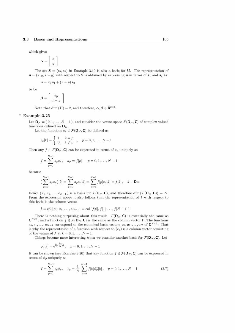
* Example 3.25

Let DN = ( 0, 1, . . . , N − 1 ), and consider the vector space F(DN ,C) of complex-valuedfunctions defined on DN .

Let the functions ep ∈ F(DN ,C) be defined as

ep[k] =

{

1, k = p0, k 6= p

, p = 0, 1, . . . , N − 1

Then any f ∈ F(DN ,C) can be expressed in terms of ep uniquely as

f =

N−1∑

p=0

apep , ap = f [p] , p = 0, 1, . . . , N − 1

because

(

N−1∑

p=0

apep )[k] =

N−1∑

p=0

apep[k] =

N−1∑

p=0

f [p]ep[k] = f [k] , k ∈ DN

Hence ( e0, e1, . . . , eN−1 ) is a basis for F(DN ,C), and therefore dim (F(DN ,C)) = N .From the expression above it also follows that the representation of f with respect tothis basis is the column vector

f = col [ a0, a1, . . . , aN−1 ] = col [ f [0], f [1], . . . , f [N − 1] ]

There is nothing surprising about this result. F(DN ,C) is essentially the same asC

N×1, and a function f ∈ F(DN ,C) is the same as the column vector f . The functionse0, e1, . . . , eN−1 correspond to the canonical basis vectors e1, e2, . . . , eN of C

N×1. Thatis why the representation of a function with respect to (ep) is a column vector consistingof the values of f at k = 0, 1, . . . , N − 1.

Things become more interesting when we consider another basis for F(DN ,C). Let

φp[k] = eip2π

Nk , p = 0, 1, . . . , N − 1

It can be shown (see Exercise 3.20) that any function f ∈ F(DN ,C) can be expressed interms of φp uniquely as

f =

N−1∑

p=0

cpφp , cp =1

N

N−1∑

k=0

f [k]φ∗p[k] , p = 0, 1, . . . , N − 1 (3.7)


Hence (φ0, φ1, . . . , φN−1 ) is also a basis for F(DN ,C), and the representation of f withrespect to (φp) is

F = col [ c0, c1, . . . , cN−1 ]

The representation of f as a linear combination of φp is known as the discrete Fourier

series of f , and the coefficients cp as the discrete Fourier coefficients of f .

As a specific example, suppose N = 4. Then the basis functions φp have the valuestabulated below.

φ0[k] φ1[k] φ2[k] φ3[k]

k = 0 1 1 1 1k = 1 1 i −1 −ik = 2 1 −1 1 −1k = 3 1 −i −1 i

Let

f [k] =

2, k = 04, k = 1

−2, k = 20, k = 3

Then the discrete Fourier coefficients of f are computed as

c0 = 14

(2 + 4 − 2 + 0) = 1

c1 = 14

(2 − 4i+ 2 + 0) = 1 − i

c2 = 14

(2 − 4 − 2 + 0) = −1

c3 = 14

(2 + 4i+ 2 + 0) = 1 + i

Hence the discrete Fourier series of f is

f = φ0 + (1 − i)φ1 − φ2 + (1 + i)φ3

and the representation of f with respect to (φp) is

F =

11 − i−11 + i

From the examples above we observe that although the representation of a vector isunique with respect to a given basis, it has a different (but still unique) representationwith respect to another basis. We now investigate how different representations ofthe same vector with respect to different bases are related.

Let R = (r1, r2, . . . , rn) and R′ = (r′1, r′2, . . . , r

′n) be two ordered bases for X.10

Suppose that a vector x has the representations

α = col [ α1, . . . , αn ] and α′ = col [ α′1, . . . , α

′n ]

10Keep in mind that even when R and R′ contain exactly the same vectors, if their orderings aredifferent then R and R′ are different.


with respect to R and R′. That is,

x =

n∑

j=1

αjrj =

n∑

i=1

α′ir

′i

Let the jth basis vector rj be expressed in terms of the vectors of R′ as

rj =

n∑

i=1

qijr′i , j = 1, . . . , n

so that it has a representation

qj = col [ q1j , . . . , qnj ] , j = 1, . . . , n

with respect to R′. Then

x =

n∑

j=1

αjrj =

n∑

j=1

αj (

n∑

i=1

qijr′i ) =

n∑

i=1

(

n∑

j=1

qijαj ) r′i =

n∑

i=1

α′ir

′i

By uniqueness of the representation of x with respect to R′, we have

α′i =

n∑

j=1

qijαj , i = 1, . . . , n

By expressing these equalities in matrix form, we observe that the representations α′

and α are related as

α′ = Q α

The matrix

Q = [q1 q2 · · · qn ] = [ qij ]n×n

which is defined uniquely by R and R′, is called the matrix of change–of–basis

from R to R′.Now interchange the roles of the bases R and R′. Let the jth basis vector r′j be

expressed in terms of the vectors of R as

r′j =

n∑

i=1

pijri , j = 1, . . . , n

so that it has a representation

pj = col [ p1j , . . . , pnj ] , j = 1, . . . , n

with respect to R. Defining

P = [p1 p2 · · · pn ] = [ pij ]n×n

to be the matrix of change–of–basis from R′ to R, we get

α = P α′

The reader might suspect that the matrices Q and P are related. Indeed, sinceα = Pα′ = PQα and α′ = Qα = QPα′ for all pairs α, α′ ∈ R

n×1, we must have

PQ = QP = In

We will investigate such matrices in Chapter 4.


Example 3.26

Consider Example 3.17. Expressing the vectors of the canonical basis E in terms of R

as

e1 = r1

e2 = −r1 + r2

e3 = −r2 + r3

we obtain the matrix of change–of–basis from E to R as

Q =

[

1 −1 00 1 −10 0 1

]

Hence the representation of a vector x = col [x1, x2, x3 ] with respect to R is related toits canonical representation x as

α = Qx =

[

1 −1 00 1 −10 0 1

][

x1

x2

x3

]

=

[

x1 − x2

x2 − x3

x3

]

which is the same as in Example 3.23.Since the representations of rj with respect to E are themselves, the matrix of change–

of–basis from R to E is easily obtained as

P = [ r1 r2 r3 ] =

[

1 1 10 1 10 0 1

]

If x has a representation

α = col [ a, b, c ]

with respect to R, then

x = ar1 + br2 + cr3 =

[

a+ b+ cb+ cc

]

= Pα

The reader should verify that QP = PQ = I .

3.4 Linear Transformations

Let X and Y be vector spaces over the same field F. A mapping A : X → Y is calleda linear transformation if for all x1,x2 ∈ X and for all c1, c2 ∈ F

A(c1x1 + c2x2) = c1A(x1) + c2A(x2) (3.8)

(3.8) is equivalent to

A(x1 + x2) = A(x1) + A(x2) (3.9)

and

A(cx) = cA(x) (3.10)

3.4 Linear Transformations 109

which are known as superposition and homogeneity, respectively. (3.9) followsfrom (3.8) on choosing c1 = c2 = 1, and (3.10) on choosing c1 = 1, c2 = 0 and x1 = x.Conversely, (3.9) and (3.10) imply that

A(c1x1 + c2x2) = A(c1x1) + A(c2x2) = c1A(x1) + c2A(x2)

X and Y are the domain and the codomain of A. A linear transformation froma vector space X into itself is called a linear operator on X.

If A : X → Y is a linear transformation then

A(0x) = 0y

which follows from (3.8) on taking c1 = c2 = 0.

Example 3.27

The zero mapping O : X → Y defined as

O(x) = 0y for all x ∈ X

is a linear transformation that satisfies (3.8) trivially.

The identity mapping I : X → X defined as

I(x) = x for all x ∈ X

is also a linear transformation, because

I(c1x1 + c2x2) = c1x1 + c2x2 = c1I(x1) + c2I(x2)

Hence I is a linear operator on X .

Example 3.28

The mapping A : R3 → R

2 defined as

A(x1, x2, x3) = (x1 + x2, x2 − x3)

is a linear transformation. For u = (u1, u2, u3), v = (v1, v2, v3) and c, d ∈ F

A(cu + dv) = A(cu1 + dv1, cu2 + dv2, cu3 + dv3)

= (cu1 + dv1 + cu2 + dv2, cu2 + dv2 − cu3 − dv3)

= c(u1 + u2, u2 − u3) + d(v1 + v2, v2 − v3)

= cA(u) + dA(v)

However, none of the mappings

B(x1, x2, x3) = (x1 + x3, x2 + 1)

C(x1, x2, x3) = (x1 + x3, x22)

D(x1, x2, x3) = (x1x3, x2)

is a linear transformation. B is not linear simply because B(0) 6= 0. The reader is urged

to explain why C and D are not linear.


Example 3.29

Let A : Fn×1 → F

m×1 be defined as A(x) = Ax, where A is an m × n matrix withelements from F. Since

A(ax + by) = aAx + bAy

A is a linear transformation. This example shows that every matrix defines a linear

transformation. Thus a linear transformation defined by an n× n matrix with elements

from F is a linear operator on Fn×1.

Example 3.30

Let X, Y, and Z be vector spaces over the same field, and let A : X → Y and B : Y → Z

be linear transformations. Then the compound mapping C : X → Z defined as

C(x) = (B ◦ A)(x) = B(A(x))

is also a linear transformation, because

C(c1x1 + c2x2) = B(A(c1x1 + c2x2))

= B(c1A(x1) + c2A(x2))

= c1B(A(x1)) + c2B(A(x2))

= c1C(x1) + c2C(x2)

* Example 3.31

In Section 2.5 we defined the differential operator D as a mapping from a set of functionsinto itself such that D(f) = f ′. We now take a closer look at D.

Recall from Example 3.8 that

C0(I,R) ⊃ C1(I,R) ⊃ · · · ⊃ C∞(I,R)

are subspaces of F (I,R). Also, if f ∈ Cm(I,R) then

f ′ ∈ Cm−1(I,R) , f ′′ ∈ Cm−2(I,R) , . . . , f (m) ∈ C0(I,R)

Hence, for any m > 1, the differential operator D is a mapping from Cm(I,R) intoCm−1(I,R), and therefore, into C0(I,R). The property in (2.34) implies that D is alinear transformation. Then, as discussed in Example 3.30, the operator D2 that isdefined in terms of D as

D2(f) = (D ◦D)(f) = D(D(f)) = D(f ′) = f ′′

is also a linear transformation. Consequently, each Dk, k = 1, . . . , n ≤ m, which can bedefined recursively as

Dk(f) = (D ◦Dk−1)(f) = D(Dk−1(f)) = D(f (k−1)) = f (k)

is a linear transformations from Cm(I,R) into Cm−k(I,R), and therefore, into C0(I,R).

Finally, an nth order linear differential operator L(D) is a linear transformation

from Cn(I,R) into C0(I,R) (see Exercise 3.31). In fact, this is precisely the reason for

calling L(D) a linear operator.


* Example 3.32

Recall that a vector x ∈ Rn×1 can also be viewed as a function f ∈ F(n,R). The linear

operator A : Rn×1 → R

n×1 defined by a matrix A ∈ Rn×n can similarly be interpreted

as a a linear operator A : F(n,R) → F(n,R) such that the image g = A(f) of a functionf is defined pointwise as

g[p] =

n∑

q=1

apqf [q] , p ∈ n

Now consider the vector space F(Z,R) of infinite sequences. We can define a linearoperator H on F(Z,R) such that if g = H(f) then

g[p] =

∞∑

q=−∞

h[p, q]f [q] , p ∈ Z (3.11)

where h[p, q] ∈ R.11 We can think of H as defined by an infinitely large matrix H withelements h[p, q] such that

...

g[−1]

g[ 0 ]

g[ 1 ]...

=

......

...

· · · h[−1,−1] h[−1, 0] h[−1, 1] · · ·

· · · h[ 0,−1] h[ 0, 0] h[ 0, 1] · · ·

· · · h[ 1,−1] h[ 1, 0] h[ 1, 1] · · ·...

......

=

...

f [−1]

f [ 0 ]

f [ 1 ]...

Let us go one step further, and consider the vector space F(R,R) of real-valuedfunctions defined on R. Now the domain of the functions is a continuum, and the infinitesummation in (3.11) must be replaced with an integral: We can then define a linearoperator H on F(R,R) such that g = H(f) is characterized by

g(t) =

∫ ∞

−∞

h(t, τ )f(τ )dτ , t ∈ R (3.12)

In the special cases when h[p, q] = h[p − q] and h(t, τ ) = h(t − τ ), the operators

defined by (3.11) and (3.12) are known as convolution, and are widely used in system

analysis.

3.4.1 Matrix Representation of Linear Transformations

Let dim (X) = n, let dim (Y) = m, let R = ( r1, . . . , rn ) and S = ( s1, . . . , sm ) beordered bases for X and Y, and let A : X → Y be a linear transformation.

Consider A(rj). Since it is a vector in Y, it has a unique representation aj ∈ Fm×1

with respect to the basis S. That is,

A(rj) =

m∑

i=1

aijsi , j = 1, . . . , n

11Of course, this definition requires that the infinite series in (3.11) converges for all p ∈ Z, whichputs some restrictions not only on h[p, q] but also on f . These technical difficulties can be workedout by restricting f to a subspace of F(Z, R) and by choosing h[p, q] suitably.


and

aj = col [ a1j , a2j , . . . , amj ] , j = 1, . . . , n

The m × n matrix

A = [a1 a2 · · · an ] = [ aij ]

which is uniquely defined by A, R and S, is called the matrix representation of a

linear transformation of A with respect to the basis pair (R,S).The significance of the matrix representation of A is that if x ∈ X has a represen-

tation α ∈ Fn×1 with respect to R and y = A(x) ∈ Y has a representation β ∈ F

m×1

with respect to S, then the two representations are related as β = Aα. To show this,suppose

x =

n∑

j=1

αjrj , y = A(x) =

m∑

i=1

βisi

Then

y =

n∑

j=1

αjA(rj) =

n∑

j=1

αj (

m∑

i=1

aijsi ) =

m∑

i=1

(

n∑

j=1

aijαj )si =

m∑

i=1

βisi

Since the representation of y in terms of si is unique, we must have

βi =n

∑

j=1

aijαj , i = 1, . . . , m

or in matrix form

β = Aα

In conclusion, not only does an m× n matrix define a linear transformation fromF

n×1 into Fm×1, but also a linear transformation from an n-dimensional vector space

X into an m-dimensional vector space Y can be represented by an m×n matrix oncea pair of bases for X and Y are fixed.12

Like the column representation of a vector with respect to basis, a linear transfor-mation has different representations with respect to different bases. If A has a repre-sentation A with respect to (R,S) and a representation A′ with respect to (R′,S′),then

A′ = QyAPx

where Qy is the matrix of change–of–basis from S to S′ in Y, and Px is the matrix ofchange–of–basis from R′ to R in X. This follows from the fact that if α and α′ arerepresentations of x with respect to R and R′, and β and β′ are representations ofy = A(x) with respect to S and S′, then

A′α′ = β′ = Qyβ = QyAα = QyAPxα′

12The question of whether a similar result can be derived for linear transformations between infinitedimensional vector spaces is beyond the scope of this book.


The relations between the vectors of X and Y and their representations are sum-marized by the diagram in Figure 3.3. From the diagram it is clear that A, QyA,APx and QyAPx all represent the same linear transformation, each with respect to adifferent pair of bases. QyA represents A with respect to (R,S′), and APx representsA with respect to (R′,S).

-

-

-�

�-

� �

�

6

6

6

6

?

?

?

?

α ∈ Fn×1

x ∈ X

α′ ∈ Fn×1

β ∈ Fm×1

y ∈ Y

β′ ∈ Fm×1

Px Qy

R′

R

S′

S

A′

A

A

Figure 3.3: Matrix representation of a linear transformation

Example 3.33

Consider the linear transformation A : Fn×1 → F

m×1 defined by a matrix Am×n ∈ Fm×n.

Let En = (en1 , . . . , e

nn ) and Em = ( em

1 , . . . , emm ) denote the canonical bases for F

n×1 and

Fm×1, respectively. Then since Aen

j = aj (the jth column of A), and since the column

representation of aj with respect to Em is itself, it follows that the matrix representation

of A with respect to the canonical bases of Fn×1 and F

m×1 is the matrix A itself.

Example 3.34

Consider the linear transformation in Example 3.28. If we choose the canonical basesE3 = ( e3

1, e32, e

33 ) and E2 = ( e2

1, e22 ) for F

3 and F2, then

A(e31) = A(1, 0, 0) = (1, 0) = e2

1

A(e32) = A(0, 1, 0) = (1, 1) = e2

1 + e22

A(e33) = A(0, 0, 1) = (0,−1) = −e2

2

and the matrix representation of A is

A =

[

1 1 00 1 −1

]

Now suppose we choose

r1 = (1, 0, 0) , r2 = (0, 1, 0) , r3 = (−1, 1, 1)

as a basis for F3, and

s1 = (1, 0) , s2 = (1, 1)


as a basis for F2. Then, since

A(r1) = A( 1, 0, 0) = (1, 0) = s1

A(r2) = A( 0, 1, 0) = (1, 1) = s2

A(r3) = A(−1, 1, 1) = (0, 0) = 0

A has the matrix representation

A′ =

[

1 0 00 1 0

]

with respect to (R,S).

Let us form the change–of–basis matrices Qy and Px. Since

e21 = s1

e22 = −s1 + s2

the matrix of change–of–basis from E2 to S in F2 is

Qy =

[

1 −10 1

]

The matrix of change–of–basis from R to E3 in F3 is readily obtained as

Px =

[

1 0 −10 1 10 0 1

]

The reader can easily verify that A′ = QyAPx.

In Example 3.30 we have seen that if A : X → Y and B : Y → Z are lineartransformations, then the mapping C : X → Z defined as

C(x) = (B ◦ A)(x) = B(A(x))

is also a linear transformation. In particular, if A : Fn×1 → F

m×1 and B : Fm×1 → F

p×1

are linear transformations defined as

A(x) = Ax , B(y) = By

where A and B are m × n and p × m matrices then C is defined as

C(x) = B(A(x)) = B(Ax) = BAx

Conversely, if X,Y and Z are finite dimensional and A and B are represented bymatrices A and B with respect to some fixed bases of X,Y and Z, then C = B ◦A isrepresented by the matrix C = BA with respect to the same bases (see Exercise 3.29).Thus a matrix product can be viewed as the representation of a linear transformationfollowed by another as illustrated in Figure 3.4.


-

-

-

-

6 6 6

? ? ?

� �

� �

6

?x ∈ X y ∈ Y z ∈ Z

α ∈ Fn×1 β ∈ F

m×1 γ ∈ Fp×1

A B

A B

R S T

C = BA

C = B ◦ A

Figure 3.4: An interpretation matrix multiplication

3.4.2 Kernel and Image of a Linear Transformation

Let A : X → Y be a linear transformation. The set

ker (A) = {x ∈ X | A(x) = 0 } ⊂ X

is called the kernel of A. Clearly, 0 ∈ ker (A). Furthermore, if x1,x2 ∈ ker (A) thenfor any c1, c2 ∈ F

A(c1x1 + c2x2) = c1A(x1) + c2A(x2) = c10 + c20 = 0

so that c1x1 + c2x2 ∈ ker (A). That is, ker (A) is closed under vector addition andscalar multiplication. Hence it is a subspace of X, which is also called the null space

of A and denoted by N (A). If it is finite dimensional, we define ν(A) = dim (ker (A))to be the nullity of A.

The set

im (A) = {y ∈ Y | y = A(x) for some x ∈ X } ⊂ Y

is called the image of A. The reader can easily show that im (A) is a subspace ofY, which is also called the range space of A and denoted as R (A). If it is finitedimensional, then we define ρ(A) = dim (im (A)) to be the rank of A.

If A : Fn×1 → F

m×1 is a linear transformation defined by an m×n matrix A, thenwe also use the notation ker (A) and im (A) to denote ker (A) and im (A).

Example 3.35

Consider the linear transformation A : R4×1 → R

3×1 defined by the matrix

A =

[

1 0 −2 −21 −1 −1 10 −1 1 3

]

= [a1 a2 a3 a4 ]

Then

ker (A) = {x ∈ R4×1 |Ax = 0 }


that is, ker (A) is precisely the set of solutions of the homogeneous system Ax = 0. Fromthe reduced row echelon form of A

A −→

[

1 0 −2 −20 1 −1 −30 0 0 0

]

we obtain two linearly independent solutions

φ1 =

2110

, φ2 =

2301

Hence ker (A) = span (φ1,φ2), and therefore, ν(A) = 2.

Clearly,

im (A) = span (a1,a2,a3,a4)

Performing elementary operations on the columns of A as

A2C1 + C3 → C3

2C1 + C4 → R+

−→

[

1 0 0 01 −1 1 30 −1 1 3

]

C2 + C3 → C3

3C2 + C4 → C4

−→

[

1 0 0 01 −1 0 00 −1 0 0

]

= [a1 a2 0 0 ]

we determine that im (A) = span (a1, a2), and hence ρ(A) = 2.

Example 3.36

Let A : R2×2 → R

2×2 be defined as

A(M) = M +M t

It is easy to see that A is a linear transformation.Since M +M t = O if and only if M is skew-symmetric,

ker (A) = span (

[

0 −11 0

]

)

and hence ν(A) = 1.Since M +M t is symmetric for any M ,

im (A) = R2×2s

where R2×2s is the subspace in Example 3.21. Hence ρ(A) = 3.

* 3.4.3 Inverse Transformations

If ker (A) = { 0 } then to every y ∈ im (A) there corresponds a unique x ∈ X suchthat A(x) = y, that is, A is one-to-one (see Exercise 3.38). It is then natural toexpect that there exists a linear transformation AL : Y → X that maps the image of


every x ∈ X back to x as illustrated in Figure 3.5. Such a linear transformation, if itexists, is called a left inverse of A.13

In general, AL is not unique because of the arbitrariness in defining AL(y) wheny /∈ im (A). However, by the very definition, it has the property that

AL(A(x)) = x for all x ∈ X

- -

-

u u u

u u

� �?

x1 x1y1 ∈ im (A)

y2 /∈ im (A) x2 (arbitrary)

A AL

AL

AL ◦ A

Figure 3.5: Left inverse of a linear transformation

Example 3.37

Let A : R2×1 → R

3×1 be defined by the matrix

A =

[

1 12 30 1

]

It can easily be verified that the only solution of Ax = 0 is the trivial solution x = 0,that is, ker (A) = { 0 }. Let

AL =

[

1 0 −10 0 1

]

Then the mapping AL : R3×1 → R

2×1 defined by AL is a left inverse of A, becauseALA = I so that

AL(A(x)) = ALAx = x for all x ∈ R2×1

The reader can verify that the matrix

A′L =

[

−1 1 −22 −1 2

]

also defines a left inverse of A.

13The proof of existence of AL in the general case is beyond the scope of this book. Left inverseof a linear transformation defined by a matrix is studied in Chepter 4.


Now suppose that im (A) = Y. Then for every y ∈ Y there exists an x ∈ X, notnecessarily unique, such that A(x) = y, that is, A is onto. We can then define a lineartransformation AR : Y → X such that AR(y) = x, where x is any fixed vector thatsatisfies A(x) = y. Because of the arbitrariness in choosing x (if there are more thanone x that satisfy A(x) = y), AR is not unique either. However, it has the propertythat

A(AR(y)) = y

for all y ∈ Y. Thus AR maps every y ∈ Y to a vector whose image is y as illustratedin Figure 3.6, and is called a right inverse of A.14

- - -

��

��

��3u u u u

u

� �?

x1

x2

y1 x1 y1

A

A

AR A

A ◦ AR

Figure 3.6: Right inverse of a linear transformation

Example 3.38

Let B : R3×1 → R

2×1 be defined by the matrix

B =

[

1 2 10 1 2

]

Since r(B) = 2, the equation Bx = y is consistent for all y, that is, im (B) = R2×1.

Let

BR =

[

1 10 −10 1

]

Then the mapping BR : R2×1 → R

3×1 defined by BR is a right inverse of B, becauseBBR = I , so that

B(BR(y)) = BBRy = y for all y ∈ R2×1

As an exercise the reader may try to find a different right inverse of B.

14Right inverse of a linear transformation defined by a matrix is also studied in Chepter 4.

3.5 Linear Equations 119

Finally, suppose that ker (A) = { 0 } and also im (A) = Y. Then A has both aleft inverse AL and a right inverse AR. Moreover, AL and AR are unique.15 SinceA(AR(y)) = y for all y ∈ Y, from the definition of left inverse it follows that

AL(y) = AL(A(AR(y))) = AR(y) for all y ∈ Y

that is, AL = AR. The unique common left and right inverse of A is simply calledthe inverse of A, denoted A−1.

In summary, if ker (A) = { 0 } and im (A) = Y for a linear transformation A :X → Y, then there exists a unique inverse transformation A−1 : Y → X such that

A−1(A(x)) = x for all x ∈ X

and

A(A−1(y)) = y for all y ∈ Y

This is somewhat an expected result, because if ker (A) = { 0 } and im (A) = Y thenA establishes a one-to-one correspondence between the elements of X and Y. Such alinear transformation is called an isomorphism, and any two vector spaces related byan isomorphism are called isomorphic. It is left to the reader to show that two finitedimensional vector spaces X and Y are isomorphic if and only if dim (X) = dim (Y)(Exercise 3.39).

Example 3.39

Let dim (X) = n, and let R be a basis for X. Let the unique representation of a vectorx ∈ X with respect to the basis R be αx ∈ F

n×1. Then the mapping A : X → Fn×1

defined as

A(x) = αx

is a linear transformation as can easily be shown using the definition of the columnrepresentation of a vector.

Since αx is uniquely defined by x, x = 0 is the only vector whose representation

is 0n×1. Hence ker (A) = {0 }. Also since every α ∈ Fn×1 is the representation of

some x ∈ X, im (A) = Fn×1. Thus A is a one-to-one mapping from X onto F

n×1 (an

isomorphism). The inverse of A is defined as A−1(αx) = x.

3.5 Linear Equations

In Chapter 1 we considered linear systems of the form

Ax = b

where A is an m × n matrix. We have seen that a general solution is of the form

x = φp + φc

15A rigorous proof of this statement is beyond the scope of this book. However, we can argue thatsince there exists no y /∈ im (A), there is no arbitrariness in AL. Also, since for any y ∈ Y, the

vector x that satisfies A(x) = y is unique, there is no arbitrariness in AR either.


where x = φp is a particular solution, and x = φc is a complementary solution thatcontains arbitrary constants and satisfies the associated homogeneous equation.

In Chapter 2 we considered first and second order linear differential equations ofthe form

L(D)(y) = u(t)

where L(D) is a linear differential operator with constant coefficients. Again, thesolution is of the form

y = φp(t) + φc(t)

where y = φp is a particular solution, and y = φc is a complementary solution.The similarities between the nature of solutions of linear differential equations and

linear systems are striking but not surprising. Both a matrix and a linear differentialoperator are linear transformations, and both a linear system and a linear differentialequation can be viewed as an equation

A(x) = y (3.13)

where A : X → Y is a linear transformation and y ∈ Y is a given vector. In the caseof linear systems X and Y are F

n×1 and Fm×1, and in the case of linear differen-

tial equations, the set of real-valued piece-wise continuous functions defined on someinterval. We now recall some definitions of Chapter 1 and Chapter 2.

An equation of the form (3.13), where A is a linear transformation, is called alinear equation. If y = 0 then the equation is homogeneous. A vector x = φ

is called a solution of (3.13) if A(φ) = y. If (3.13) has no solution, it is said to beinconsistent. Clearly, (3.13) is consistent if and only if y ∈ im (A).

Consider the homogeneous linear equation

A(x) = 0 (3.14)

which is consistent as x = 0 is a trivial solution. Clearly, the set of all solutions of(3.14) is ker (A). Suppose that dim (ker (A)) = ν(A) = ν, and let {φ1, . . . , φν } be abasis for ker (A). Then any solution of (3.14) can be expressed in terms of the basisvectors as

x = c1φ1 + · · · + cνφν (3.15)

for some choice of the constants c1, . . . , cν .Now consider the non-homogeneous linear equation (3.13). Assume that y ∈

im (A), so that it has at least one particular solution x = φp. Then for arbitraryc1, . . . , cν

x = φp + c1φ1 + · · · + cνφν (3.16)

is also a solution, because

A(φp + c1φ1 + · · · + cνφν) = A(φp) +ν

∑

i=1

ciA(φi) = y +ν

∑

i=1

ci0 = y

Conversely, if x = φ is any solution of (3.13), then since

A(φ − φp) = A(φ) −A(φp) = y − y = 0


φ − φp is a solution of the associated homogeneous equation (3.14), and therefore,can be expressed as in (3.15). This, in turn, implies that φ is of the form (3.16). Thus(3.16) characterizes the solution set of (3.13), and is called a general solution.

Note that neither φp nor φi, i = 1, . . . , ν, are unique. If φ′p is another particular

solution, and φ′i, i = 1, . . . , ν, form another basis for ker (A), then

x = φ′p + c′1φ

′1 + · · · + c′νφ

′ν (3.17)

is also a general solution. Although the expressions in (3.16) and (3.17) are different,they nevertheless define the same family of solutions (see Exercise 3.41).

Example 3.40

Consider the linear system

[ 1 2 3 ]

[

x1

x2

x3

]

= 2

whose coefficient matrix is already in reduced row echelon form.Following the standard procedure of Chapter 1, a general solution is obtained as

x =

[

200

]

+ c1

[

−210

]

+ c2

[

−301

]

where φp = col [ 2, 0, 0 ] is a particular solution, and φ1 = col [−2, 1, 0 ] and φ2 =col [−3, 0, 1 ] form a basis for the kernel of the coefficient matrix.

On the other hand, φ′p = col [ 0, 1, 0 ] is also a particular solution (obtained from

the general solution above by choosing c1 = 1 and c2 = 0), and φ′1 = col [−2, 1, 0 ] and

φ′2 = col [ 0,−3, 2 ] form another basis for the kernel of the coefficient matrix. Thus

x =

[

010

]

+ c′1

[

−210

]

+ c′2

[

0−3

2

]

is also a general solution.

The reader can verify that any solution obtained from the second expression by

choosing arbitrary values for c′1 and c′2 can also be obtained from the first expression by

choosing c1 = 1 + c′1 − c′2 and c2 = 2c′2, and vice versa.

Linear equations of the form (3.13) are not limited to linear differential equationsand linear systems. In the following two examples, we consider different types oflinear equations.

Example 3.41

Consider the linear equation

A(M) = M +M t = N =

[

6 22 −4

]

where A is the linear transformation considered in Example 3.36. Since the matrix onthe right-hand side of the above equation is symmetric, it is in im (A), and hence, theequation is consistent.


A particular solution can be obtained by inspection to be

Mp =1

2N =

[

3 11 −2

]

(Since N is symmetric, then so is Mp, and hence Mp +M tp = 2Mp = N .)

The general solution can then be obtained by complementing Mp with ker (A), whichhas already been characterized in Example 3.36, as

M =

[

3 11 −2

]

+ c

[

0 −11 0

]

Thus

M =

[

3 02 −2

]

is also a solution obtained from the general solution with c = 1. Indeed

M +M t =

[

3 02 −2

]

+

[

3 20 −2

]

=

[

6 22 −4

]

= N

Example 3.42

Suppose that we are interested in finding a sequence f ∈ F(N,C) which satisfies anequation of the form

f [k + 2] + a1f [k + 1] + a2f [k] = u[k] , k ≥ 1 (3.18)

where a1, a2 are fixed (complex) coefficients, and u ∈ F(N,C) is a given sequence. Suchan equation is called a (second order) difference equation.16

Obtaining a solution to a difference equation is easy: Choose f [1] and f [2] arbitrarily,and calculate f [3], f [4], etc., recursively from (3.18). Thus

f [1] = c1

f [2] = c2

f [3] = −a2f [1] − a1f [2] + u[1] = −a2c1 − a1c2 + u[1]

f [4] = −a2f [2] − a1f [3] + u[2] = (a1a2)c1 + (a21 − a2)c2 + u[2] − a1u[1]

and so on. Certainly, any term of a solution sequence can be obtained after sufficientnumber of substitutions. However, it would be useful to have a formula for the kth term,which could be evaluated without working out all the intermediate terms.

Let us try to formulate the problem as a linear equation. For this purpose we definea shift operator ∆ : F(N,C) → F(N,C) as

(∆f)[k] = f [k + 1] , k ∈ N

Defining ∆2,∆3, etc., similar to the powers of the differential operator D, the differenceequation in (3.18) can be expressed as

L(∆)(f) = u[k] (3.19)

where

L(∆) = ∆2 + a1∆ + a2I

16Note that the recursion relations we considered in Section 2.8 in connection with numericalsolution of differential equations are difference equations with specified initial conditions.


is a polynomial shift operator on F(N,C).

It is left to the reader to show that L(∆) is a linear operator on F(N,C). Hencethe linear difference equation (3.18) is a linear equation. Then it must have a generalsolution of the form

f = φp[k] + φc[k]

where φp is any particular solution sequence, and φc is a complementary solution sequenceexpressed as a linear combination of the basis vectors of ker (L(∆)).

To be more specific, let us consider the difference equation

f [k + 2] −5

6f [k + 1] +

1

6f [k] = 1 , k ∈ N

or in operator notation

(∆2 −5

6∆ +

1

6I)(f) = 1 , k ∈ N

Since the right-hand side of the given equation is a constant, we suspect that aconstant sequence f [k] = C might be a solution. Substituting the assumed solution intothe equation, and noting that ∆2(C) = ∆(C) = C, we get

C − (5/6)C + (1/6)C = (1/3)C = 1

giving C = 3. A particular solution is thus obtained as φp[k] = 3.

To find the complementary solution, we try a sequence of the form f [k] = zk. Sub-stituting the trial solution into the homogeneous equation, we get

L(∆)(zk) = (zk+2 − (5/6)zk+1 + (1/6)zk) = 0

or equating the corresponding terms

zk+2 − (5/6)zk+1 + (1/6)zk = zk(z2 − (5/6)z + (1/6)) = 0

From the last equation, we observe that φ[k] = zk is a solution if and only if z is a rootof the characteristic equation

z2 − (5/6)z + (1/6) = 0

Since the characteristic equation has two real roots, µ1 = 1/2 and µ2 = 1/3, each of thesequences

φ1[k] = (1/2k) and φ2[k] = (1/3k)

is a solution of the homogeneous equation. It can be shown that φ1 and φ2 are linearlyindependent sequences, and thus form a basis for ker (L(∆)). The general solution of thenon-homogeneous difference equation is thus obtained as

f = φ[k] = 3 + c1/2k + c2/3

k , c1, c2 ∈ C


* 3.6 Direct Sum and Projections

Consider an arbitrary vector x = (x1, x2, x3) ∈ R3. In terms of the canonical basis

vectors e1 = (1, 0, 0), e2 = (0, 1, 0) and e3 = (0, 0, 1), x can be expressed uniquely as

x = x1e1 + x2e2 + x3e3 (3.20)

Let Ui = span (ei), i = 1, 2, 3, be the one-dimensional subspaces of R3 defined by

the canonical basis vectors. (They represent the x, y and z axes in the the xyz space).Then we can interpret (3.20) as

x = u1 + u2 + u3

which is a decomposition of x into three components u1 = x1e1,u2 = x2e2,u3 = x3e3

in the subspaces U1,U2,U3.Now let V1 = span (e1, e2) and V2 = span (e3), where V1 is a two-dimensional

subspace (the xy plane) and V2 is a one-dimensional subspace (the z axis). Then(3.20) can also be written as

x = v1 + v2

which gives a decomposition of x into two components v1 = x1e1+x2e2 and v2 = x3e3

in the subspaces V1 and V2. Obviously, these components are uniquely determinedby x and the subspaces V1 and V2.

This example suggests that the idea of decomposing a vector into componentsalong the one-dimensional subspaces defined by a given basis can be generalized to adecomposition into components in higher dimensional subspaces.

Let U1,U2, . . . ,Uk be subspaces of a vector space X. Their algebraic sum isdefined as

k∑

i=1

Ui = {x |x =

k∑

i=1

ui,ui ∈ Ui, i = 1, . . . , k }

It is easy to show that the algebraic sum is also a subspace of X.The subspaces U1,U2, . . . ,Uk are said to be linearly independent if for ui ∈

Ui, i = 1, . . . , k

k∑

i=1

ui = 0

is satisfied only when ui = 0, i = 1, . . . , k.If U1,U2, . . . ,Uk are said to be linearly independent their algebraic sum is called

a direct sum, denoted⊕k

i=1Ui.

Note that algebraic sum of a family of subspaces is a generalization of the conceptof span of a set of vectors. Similarly, linear independence of a family of subspacesis a generalization of the concept of linear independence of a set of vectors. Thefollowing theorem characterizes two linearly independent subspaces. The extensionof the theorem to more than two subspaces is left to the reader as an exercise (seeExercise 3.43).

3.6 Direct Sum and Projections 125

Theorem 3.2 Let R = { r1, r2, . . . } and S = { s1, s2, . . . } be bases for the subspacesU and V. Then the following are equivalent.

a) U and V are linearly independent.

b) U ∩V = { 0 }.

c) T = { r1, r2, . . . , s1, s2, . . . } is a basis for U + V.

Proof We will show that (a) ⇒ (b) ⇒ (c) ⇒ (a).

(a) ⇒ (b):

By contradiction. Suppose that there exists 0 6= x ∈ U ∩ V. Let u = x ∈ U,v =−x ∈ V. Then u 6= 0 6= v and u + v = x − x = 0.

(b) ⇒ (c):

By contradiction. Since span (T) = U + V, if T is not a basis for U + V then itmust be linearly dependent, in which case there exist scalars αi and βj , not all zero,such that

∑

i

αiri +∑

j

βjsj = 0

Let

x =∑

i

αiri = −∑

j

βjsj

Then x ∈ U ∩ V, and x 6= 0 as R and S are linearly independent.

(c) ⇒ (a):

Suppose u + v = 0 for some

u =∑

i

αiri and v =∑

j

βjsj

that is,∑

i

αiri +∑

j

βjsj = 0

Since T is a basis, we must have αi = 0 for all i implying u = 0, and also βj = 0 forall j implying v = 0.

Example 3.43

In R3, let

U1 = span (e1, e2) , U2 = span (e2, e3) , U3 = span (e3)

where e1, e2, e3 are the canonical basis vectors. Then

U1 + U2 = U1 + U3 = span (e1, e2, e3) = R3

U1 and U2 are not linearly independent, because e2 ∈ U1 ∩ U2. However, U1 andU3 are linearly independent, because {e1, e2, e3} is a basis for U1 + U3. Hence

R3 = U1 ⊕U3

The reader can interpret these findings by identifying R3 with the xyz space, and

U1,U2 and U3 with the xy plane, yz plane, and the z axis respectively.


From Theorem 3.2 it is clear that if T = { t1, t2, . . . , tn } is a basis for X, parti-tioned arbitrarily into two disjoint sets, say

R = { t1, t2, . . . , tk } and S = { tk+1, tk+2, . . . , tn }

then

X = span (R) ⊕ span (S)

On the other hand, if R = { r1, r2, . . . , rk } is a basis for a k-dimensional subspace U,then by Corollary 3.2, it can be completed to a basis by including n−k more vectors.Let these additional vectors form a set S, and let V = span (S). Then X = U ⊕ V.The subspace V thus constructed is called a complement of U. Since S can bechosen in many different ways, complement of U is not unique. For example, for anyvector v = (a, b, c) with c 6= 0, V = span (v) is a complement of U1 in Example 3.43,and in particular, so is U3. However, all complements of U must have the samedimension.

We also observe that if X is finite dimensional and is decomposed into a directsum as X = U ⊕ V then

dim (X) = dim (U) + dim (V)

Let X = U ⊕ V, and let R = ( r1, . . . , rk ) and S = ( s1, . . . , sn−k ) be orderedbases for U and V. Since T = R ∪ S is a basis for X, any vector x ∈ X can beexpressed as

x =

k∑

i=1

αiri +

n−k∑

j=1

βjsj = u + v (3.21)

The vectors u ∈ U and v ∈ V, which are uniquely defined by x, are called thecomponents of x in U and V.

Let P : X → X be a mapping which maps every vector in X to its component inU, that is,

P(x) = u

P is called a projection on U along V. It is left to the reader to show that

a) P is a linear transformation

b) im (P) = U

c) ker (P) = V

The reader should note that the mapping Q : X → X defined as Q(x) = v is also aprojection (on V along U).

The matrix P that represents P with respect to the basis T is called a projection

matrix. Since

P(P(x)) = P(u) = u = P(x)

for any x ∈ X, it follows that P 2α = Pα for any α ∈ Fn×1 that stands for the column

representation of some vector. Thus if P is a projection matrix then P 2 = P . Such amatrix is called idempotent. Conversely, if P is an n× n idempotent matrix, then

Fn×1 = im (P ) ⊕ ker (P )

and P defines a projection in Fn×1 on im (P ) along ker (P ) (see Exercise 3.51).

3.6 Direct Sum and Projections 127

Example 3.44

In Example 3.43, the projection on U1 along U3 is defined by the matrix

P =

[

1 0 00 1 00 0 0

]

and the projection on U3 along U1 is defined by the matrix

Q =

[

0 0 00 0 00 0 1

]

Note that P 2 = P and Q2 = Q.Now consider the matrix

R =1

3

[

2 1 −11 2 1

−1 1 2

]

Since R is idempotent, it defines a projection in R3×1 on

im (R) = span (

[

110

]

,

[

011

]

) = span (u1,u2 )

along

ker (R) = span (

[

1−1

1

]

) = span (u3 )

The components of an arbitrary vector x = col [ a, b, c ] in im (R) and ker (R) are

u = Rx =1

3

[

2a + b− ca+ 2b+ c

−a+ b+ 2c

]

=2a+ b− c

3u1 +

−a+ b+ 2c

3u2

and

v = (I −R)x =1

3

[

a− b+ c−a+ b− ca− b+ c

]

=a− b+ c

3u3

Example 3.45

In C[s], let

Ce[s] = { p(s) = p0 + p1s2 + · · · + pms

2m | m = 0, 1, . . . }

Co[s] = { q(s) = q0s+ q1s3 + · · · + qms

2m+1 | m = 0, 1, . . . }

Then C[s] = Ce[s] ⊕ Co[s].If

r(s) = r0 + r1s+ r2s2 + · · · + r2n+1s

2n+1

then

re(s) = r0 + r2s2 + · · · + r2ns

2n

is the projection of r on Ce[s] along Co[s].

This example illustrates that direct sum decomposition and projections are not lim-

ited to finite dimensional vector spaces.


3.7 Exercises

1. Prove properties (a-f) on p.87 of a vector space.

2. Show that a plane through the origin is a subspace of R3.

3. Write down the equation of a line passing through two given points p,q ∈ Rn. Under

what conditions on p,q does the line represent a subspace?

4. Discuss how an m× n real matrix A can be interpreted as a function f : n → Rm×1.

5. Show that if U and V are subspaces of X, then so is U∩V. Is U∪V also a subspace?

6. Show that span (span (R)) = span (R) for any subset R ⊂ X.

7. Prove facts (a-c) on p.93 concerning linear independence.

8. Let R be a finite set of vectors and let R′ be obtained from R by a single Type I orType II elementary operation.

(a) Explain why span (R′) = span (R).

(b) Explain why R′ is linearly independent if and only if R is.

9. Show that C is a vector space over R, and find a basis for it.

10. Show that the set of all 3× 3 real skew-symmetric matrices is a subspace of R3×3, and

find a basis for it.

11. Show that the set R = { r0, r1, . . . } in Example 3.18 is a basis for R[s].

12. An n× n matrix N is said to be nilpotent of index k if Nk = O but Nk−1 6= O.

(a) Let v be such that Nk−1v 6= 0. Show that the vectors v, Nv, . . . , Nk−1v arelinearly independent.

(b) Show that the index of nilpotency cannot exceed n.

13. Suppose R is linearly independent, and x /∈ span (R). Show that R ∪ {x } is alsolinearly independent. Hint: Consider a finite subset S ⊂ R ∪ {x }. If x /∈ S then S ⊂R, and therefore S must be linearly independent. If x ∈ S then S = { r1, . . . , rk,x }for some r1, . . . , rk ∈ R.

14. Since the set R = { r1, . . . , rk, rk+1, . . . , rk+n } in the proof of Corollary 3.2(b) islinearly dependent, there exist some c1, . . . , cn+k, not all zero, such that

n+k∑

i=1

ciri = 0

Show that at least one of ck+1, . . . , cn+k must be nonzero. Explain why this impliesthat the set obtained by deleting the corresponding vector from R includes the firstk vectors and still spans X. On the basis of this reasoning, explain also why thealgorithm in the proof of Corollary 3.2(a) reduces R to a basis that includes R1.

15. Let U = span (u1,u2, ..., up) and V = span (v1,v2, ...,vq) be subspaces of Rn×1. Give

an algorithm to obtain a basis for U ∩ V.

16. In a two-dimensional vector space X, a vector x has the representation α = col [ 1,−1 ]with respect to some ordered basis R = ( r1, r2 ). Let

r′1 = r1 + r2 and r

′2 = r1 + 2r2

(a) Show that R′ = ( r′1, r′2 ) is also a basis for X.

(b) Find the matrix of change–of–basis Q from R to R′, and the matrix of change–of–basis P from R′ to R. Verify that QP = PQ = I .

3.7 Exercises 129

(c) Obtain the representation α′ of x with respect to R′.

17. Refer to Example 3.25. Let N = 4.

(a) Find the matrix of change–of–basis Q from (ep) to (φp).

(b) Verify that F = Q f for the sequence f considered in the example.

18. Let f = (3,−1,−3, 5, 3, 5) ∈ F(D6,C).

(a) Compute the discrete Fourier coefficients of f .

(b) Verify your result by using the MATLAB commands

f=[3 -1 -3 5 3 5];

c=fft(f)

19. Refer to Example 3.25.

(a) Show that

ψp[k] =

1, p = 0

cos π2 k p = 1

sin π2 k p = 2

cos πk p = 3

is also a basis for F(D4,C).

(b) Find the representation of f with respect to (ψp).

20. Show (3.7) for f ∈ F(DN ,C). Hint: Each of the complex numbers

sp = eip

2π

N , p = 0, 1, . . . , N − 1

satisfies

sNp = 1

Use this fact to show that

N−1∑

p=0

eip

2π

Nq

=

{

N, q = 00, q 6= 0

21. Consider F(D,R) with D = { 1, 2, 3 }.

(a) Show that (g1, g2, g3), where

g1[k] = 1 , k = 1, 2, 3

g2[k] =

{

1, k = 1, 20, k = 3

g3[k] =

{

0, k = 11, k = 2, 3

is a basis for F(D,R).

(b) Find the column representation of

f [k] = k , k = 1, 2, 3

with respect to (g1, g2, g3).


22. Prove that F(N,R) is infinite dimensional. Hint: Assume that it has a finite dimension,say, M , and try to find a subspace of F(N,R) with dimension larger than M .

23. Let A : R2×1 → R

2×1 be a linear transformation defined by the matrix

A =

[

2 11 2

]

Can you find a basis for R2×1 with respect to which A is represented by a diagonal

matrix?

24. Let A : R3 → R

2 be defined as A(x, y, z) = (x+ y, y− 2z). Choose arbitrary bases forR

3 and R2 (other than the canonical bases) and obtain the matrix representation of

A with respect to these bases.

25. Let

R3[s] = { p(s) = p0 + p1s+ p2s2 + p3s

3 | p0, p1, p2, p3 ∈ R }

(a) Find a basis R for R3[s].

(b) Find the column representation of q(s) = 1 + s2 − 2s3 with respect to R.

(c) Let A : R3[s] → R3[s] be defined as A(p) = p′, where p′ denotes the derivativeof p. Show that A is a linear transformation, and find its matrix representationwith respect to R.

26. Let A : R2×2 → R

2×2 be defined as A(X) = CX, where

C =

[

0 1−2 3

]

Find the matrix representation of A with respect to the basis in Example 3.21.

27. (a) Show that the matrices

M1 =

[

1 00 0

]

, M2 =

[

0 00 1

]

, M3 =

[

0 11 0

]

, M4 =

[

0 1−1 0

]

form an ordered basis M = (M1,M2,M3,M4) for R2×2.

(b) Let A : R2×2 → R

2×2 be defined as in Example 3.36. Find Y = A(X) for

X =

[

1 02 −3

]

(c) Find the column representations α and β of X and Y with respect to M.

(d) Find the matrix representation A of A with respect to M, and show that β = Aα.

28. In special theory of relativity, the space and time coordinates of an object measuredin two coordinate systems moving in the x direction at a constant relative speed arerelated by the Lorentz transformation

L(v) : x′ = kv(x− vt)

t′ = kv(−v

c2x+ t)

where c is the speed of light, v < c is the relative speed of the coordinate systems, andkv = 1/

√

1 − (v/c)2.

(a) Show that the Lorentz transformation is a linear transformation from R2 into

itself, mapping (x, t) to (x′, t′).

3.7 Exercises 131

(b) Find the matrix representation L(v) of the Lorentz transformation with respectto the canonical basis in R

2.

(c) Show that L(u)L(v) = L(w) for some w, and find w in terms of u and v.

29. Let R = ( r1, . . . , rn ),S = ( s1, . . . , sm ) and T = ( t1, . . . , tp ) be bases for the vec-tor spaces X,Y and Z, respectively, and let A : X → Y and B : Y → Z be lineartransformations. Show that if A and B are represented by the matrices A and B withrespect to the given bases, then C : X → Z defined as C(x) = B(A(x)) is representedby the matrix C = BA. Hint: By definition

A(rj) =

m∑

k=1

akjsk , B(sk) =

p∑

i=1

bikti , C(rj) =

p∑

i=1

cijti

Find an expression for cij in terms of bik and akj .

30. Let X and Y be vector spaces over the same field F.

(a) Show that the set of all linear transformations from X into Y is also vector spaceover F. This vector space is denoted by L(X,Y). Define clearly the additionand scalar multiplication operations on L(X,Y), as well as the null vector andthe additive inverse.

(b) Find dim (L(X,Y)) if dim (X) = n and dim (Y) = m.

31. In the light of the previous exercise, explain why L(D) is a linear transformation fromCn(I,R) into C0(I,R).

32. Let

f [k] =

{

1 + (−1)k, k ≥ 00, k < 0

(a) Find the sequence g defined by (3.11) for

h[p, q] =

{

1/2, q = p or q = p− 10, q 6= p, p− 1

Plot f and g pointwise for −2 ≤ k ≤ 5.

(b) Repeat part(a) for

h[p, q] =

{

1/2, q = p−1/2, q = p− 1

0, q 6= p, p− 1

33. Let

h(t, τ ) =

{

1, t− 1 < τ < t0, τ < t− 1 or τ > t

and

f(t) =

{

e−t, t > 00, t < 0

Find the function g defined by (3.12). Plot f and g for −1 ≤ t ≤ 5.

34. Show that if A : X → Y is a linear transformation, then im (A) is a subspace of Y.

35. Let A : R3 → R

3 be defined as A(x, y, z) = (x+ y, x+ 2z, 2x+ y+ 2z). Find bases forim (A) and ker (A).


36. Let A be the LT defined in Exercise 3.25. Find bases for for im (A) and ker (A).

37. Find a 3 × 3 real matrix A such that 0 6= ker (A) ⊂ im (A) 6= R3×1.

38. Let A : X → Y be a linear transformation.

(a) Show that if {A(x1), . . . ,A(xk) } is linearly independent, then so is {x1, . . . ,xk }.

(b) Show that A is one-to-one if and only if ker (A) = {0}. Hint: Suppose thatcorresponding to some y ∈ im (A) there exist x1 6= x2 such that A(x1) =A(x2) = y. Let x = x1 − x2 6= 0, and consider A(x).

(c) Show that if A is a one-to-one LT, and {x1, . . . ,xk } is linearly independent,then {A(x1), . . . ,A(xk) } is also linearly independent.

39. (a) Let dim (X) = n and let A : X → Y be an isomorphism. Prove that dim (Y) = n.Hint: Let ( r1, . . . , rn ) be a basis for X. Show that (A(r1), . . . ,A(rn) ) is a basisfor Y.

(b) Let X and Y be vector spaces over F, and let ( r1, . . . , rn ) and ( s1, . . . , sn ) bebases for X and Y. Define A : X → Y such that

x =

n∑

i=1

ciri =⇒ A(x) =

n∑

i=1

cisi

Show that A is an isomorphism.

40. Let A : X → Y, where X,Y are finite dimensional. Show that there exist bases forX,Y with respect to which A has a matrix representation

A =

[

I 00 0

]

41. Let φp and φ′p be any two particular solutions of (3.13), and let ( φ1, . . . ,φν ) and

( φ′1, . . . ,φ

′ν ) be any two bases for ker (A). Show that

x = φp + c1φ1 + c2φ2 + · · · + cνφν

and

x = φ′p + c′1φ

′1 + c′2φ

′2 + · · · + c′νφ

′ν

define the same family of solutions, and therefore, are both general solutions. Hint:Since φ′

p is a solution, it is a member of the first family. Also, each φ′j can be expressed

in terms of φi , i = 1, . . . , ν.

42. Show that the polynomial shift operator L(∆) in Example 3.42 is a linear operator onthe vector space of F(N,C).

43. State and prove Theorem 3.2 for more than two subspaces Ui, i = 1, . . . , k. Hint: Part(b) will be

(b)Ui ∩∑

j 6=iUj = {0 } , i = 1, . . . , k

44. (a) Show that the set U = { col [ x, x, y ] | x, y ∈ R } is a subspace of R3×1.

(b) Find a basis for U. What is the dimension of U?

(c) Obtain the representation of the vector u = col [ 1, 1, 2 ] ∈ U with respect to thebasis chosen in (b).

(d) Characterize another subspace V such that R3×1 = U ⊕ V

3.7 Exercises 133

45. Let U = span (u1,u2), where

u1 =

[

120

]

, u2 =

[

101

]

(a) Characterize a subspace V such that U ⊕ V = R3×1.

(b) Find the projection of x = col [ 0, 2, 1 ] on U along V.

(c) Find a matrix P such that for any x ∈ R3×1, Px is the projection of x on U.

46. Let U = span (u1,u2), V = span (v1,v2), where

u1 =

1111

, u2 =

0011

, v1 =

0111

, v2 =

0001

(a) Show that U ⊕ V = R4×1.

(b) Find the projection of x = col [x1, x2, x3, x4 ] on U along V.

(c) Construct a matrix P such that for any x ∈ R4×1, the projection of x on U along

V is Px.

47. Let X be the set of all semi-infinite sequences f ∈ F(N,R) such that

f [k + 2] = f [k] + f [k + 1] , k ∈ N

Such a sequence is known as a Fibonacci sequence.

(a) Show that X is a vector space over R.

(b) Show that the sequences

s1 = (1, 1, 2, 3, 5, 8, 13, ...) and s2 = (−1, 1, 0, 1, 1, 2, 3, ...)

form a basis for X.

(c) Find the projection of the sequence f = (1, 2, 3, 5, 8, 13, ...) on span (s2) alongspan (s1).

(d) Let A : X → R2 be defined as A(f) = (f [3], f [4]). Find the matrix representation

of A with respect to the basis of X in part (b) and the canonical basis of R2.

48. Let X = U ⊕ V, and let R = ( r1, . . . , rk ) and S = ( s1, . . . , sn−k ) be bases for U

and V so that T = ( r1, . . . , rk, s1, . . . , sn−k ) is a basis for X. Let P be a projectionon U along V.

(a) Find the matrix representation of P with respect to T if P is interpreted as aLT from X into itself.

(b) Find the matrix representation of P with respect to (T,R) if P is interpreted asa LT from X into U.

49. Show that P : R2 → R

2 defined as

P(α, β) = (α− β

2,β − α

2)

is a projection. Characterize im (P) and ker (P). Illustrate the decomposition of avector into components in im (P) and ker (P) with the help of a picture.

50. Prove facts (a-c) on p.126 concerning a projection.


51. Show that if P ∈ Fn×n is idempotent, then it defines a projection on im (P ) along

ker (P ). Hint: For any x ∈ Fn×1, let u = Px ∈ im (P ) and v = (I − P )x, and show

that v ∈ ker (P ).

52. A projection in the xyz space projects every point onto the plane described by

x+ y + z = 0

along its normal n = col [ 1, 1, 1 ].

(a) Find the projection u of the point x = col [ a, b, c ] on the plane.

(b) Find a matrix P such that u = Px.

(c) Verify that P 2 = P .

Documents

Chapter 3 Vector Spaces and Linear Transformationskilyos.ee.bilkent.edu.tr/~sezer/EEE501/Chapter3.pdf · Chapter 3 Vector Spaces and Linear Transformations 3.1 Vector Spaces Recall