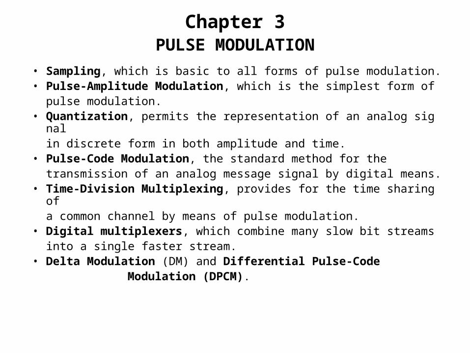
Chapter 3PULSE MODULATION

• Sampling, which is basic to all forms of pulse modulation.• Pulse-Amplitude Modulation, which is the simplest form of

pulse modulation.• Quantization, permits the representation of an analog signal

in discrete form in both amplitude and time.• Pulse-Code Modulation, the standard method for the

transmission of an analog message signal by digital means.• Time-Division Multiplexing, provides for the time sharing of

a common channel by means of pulse modulation.• Digital multiplexers, which combine many slow bit streams

into a single faster stream.• Delta Modulation (DM) and Differential Pulse-Code Modulation (DPCM).

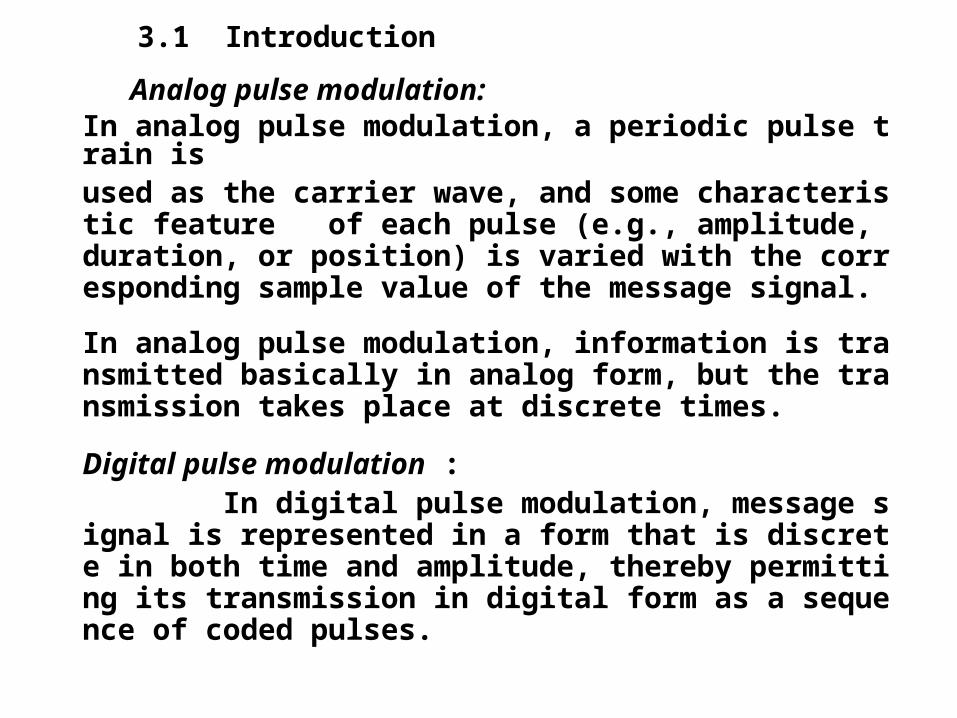
3.1 Introduction

Analog pulse modulation:

In analog pulse modulation, a periodic pulse train is used as the carrier wave, and some characteristic feature of each pulse (e.g., amplitude, duration, or position) is varied with the corresponding sample value of the message signal.

In analog pulse modulation, information is transmitted basically in analog form, but the transmission takes place at discrete times.

Digital pulse modulation : In digital pulse modulation, message signal is represented in a form that is discrete in both time and amplitude, thereby permitting its transmission in digital form as a sequence of coded pulses.

3.2 Sampling Process

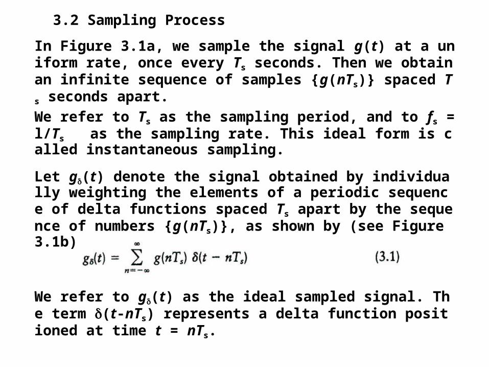
In Figure 3.1a, we sample the signal g(t) at a uniform rate, once every Ts seconds. Then we obtain an infinite sequence of samples {g(nTs)} spaced Ts seconds apart.

We refer to Ts as the sampling period, and to fs = l/Ts as the sampling rate. This ideal form is called instantaneous sampling.

Let g(t) denote the signal obtained by individually weighting the elements of a periodic sequence of delta functions spaced Ts apart by the sequence of numbers {g(nTs)}, as shown by (see Figure 3.1b)

We refer to g(t) as the ideal sampled signal. The term (t-nTs) represents a delta function positioned at time t = nTs.

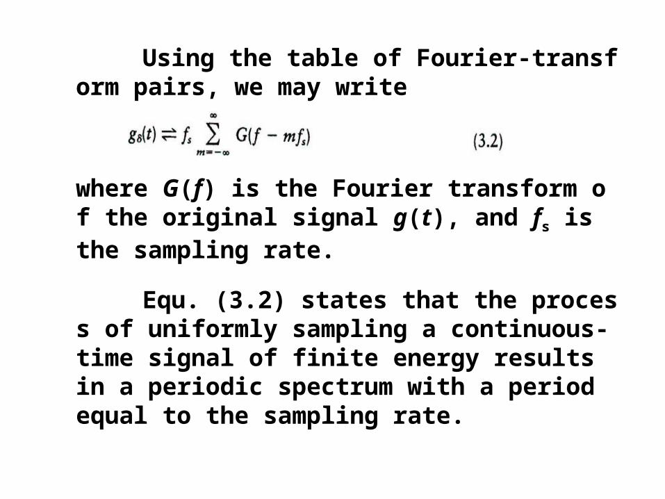
Using the table of Fourier-transform pairs, we may write

where G(f) is the Fourier transform of the original signal g(t), and fs is the sampling rate.

Equ. (3.2) states that the process of uniformly sampling a continuous-time signal of finite energy results in a periodic spectrum with a period equal to the sampling rate.

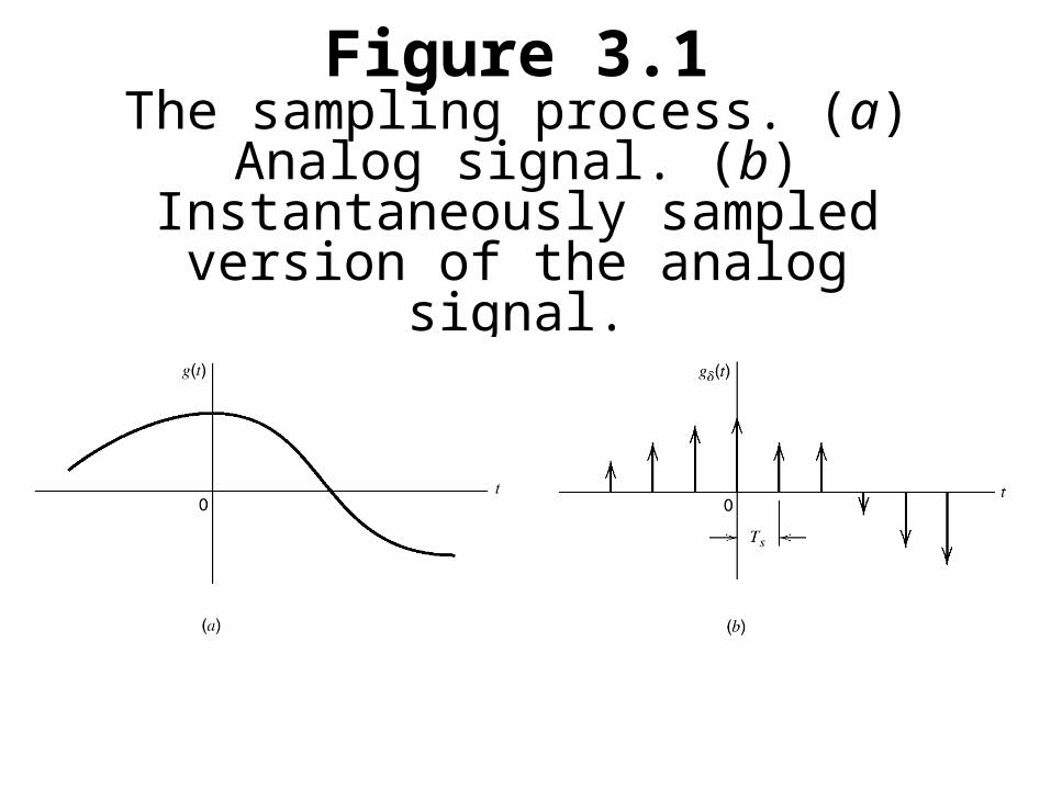
Figure 3.1The sampling process. (a) Analog

signal. (b) Instantaneously sampled version of the analog signal.

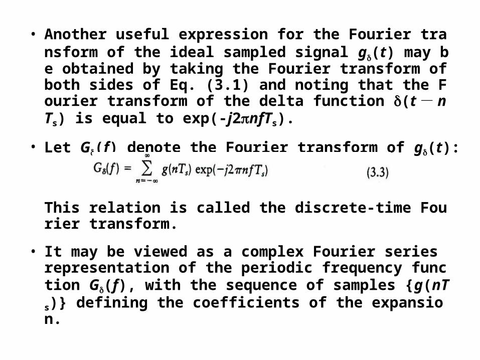
• Another useful expression for the Fourier transform of the ideal sampled signal g(t) may be obtained by taking the Fourier transform of both sides of Eq. (3.1) and noting that the Fourier transform of the delta function (t－ nTs) is equal to exp(-j2nfTs).

• Let G(f) denote the Fourier transform of g(t):

This relation is called the discrete-time Fourier transform.

• It may be viewed as a complex Fourier series representation of the periodic frequency function G(f), with the sequence of samples {g(nTs)} defining the coefficients of the expansion.

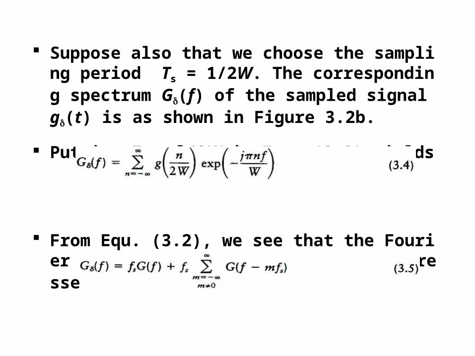
Suppose also that we choose the sampling period Ts = 1/2W. The corresponding spectrum G(f) of the sampled signal g(t) is as shown in Figure 3.2b.

Putting Ts = l/2W in Equ. (3.3) yields

From Equ. (3.2), we see that the Fourier transform of g(t) may also be expressed as

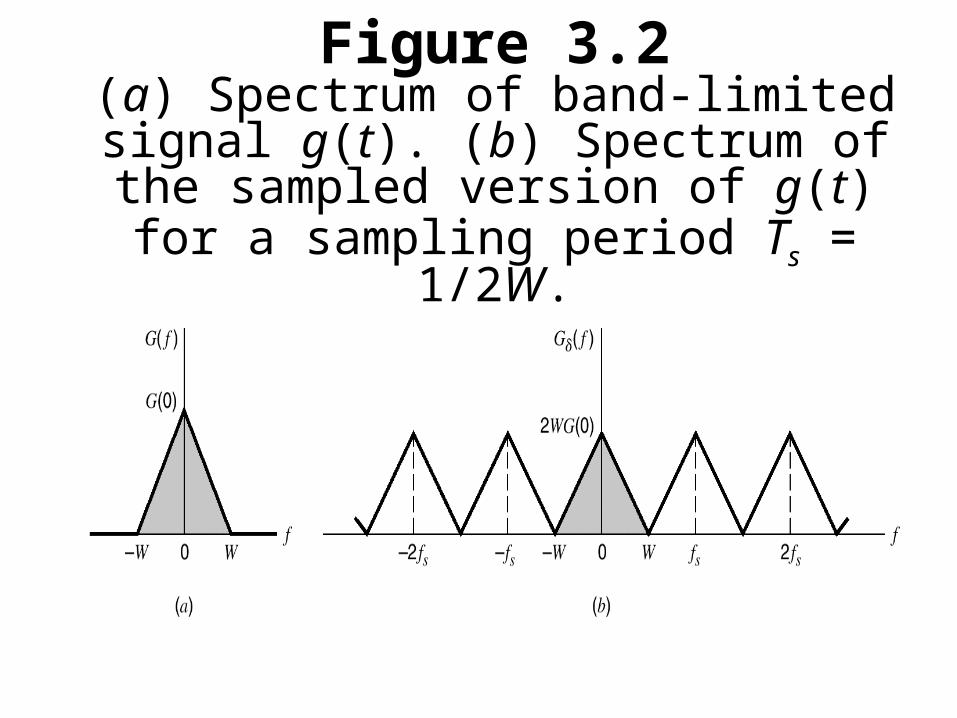
Figure 3.2(a) Spectrum of band-limited signal g(t). (b) Spectrum of the sampled version of g(t) for a sampling period Ts = 1/2W.

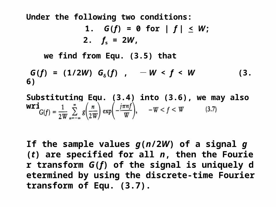
Under the following two conditions:

1. G(f) = 0 for | f | < W;

2. fs = 2W,

we find from Equ. (3.5) that

G(f) = (1/2W) Gδ(f) , －W < f < W (3.6)

Substituting Equ. (3.4) into (3.6), we may also write

If the sample values g(n/2W) of a signal g(t) are specified for all n, then the Fourier transform G(f) of the signal is uniquely determined by using the discrete-time Fourier transform of Equ. (3.7).

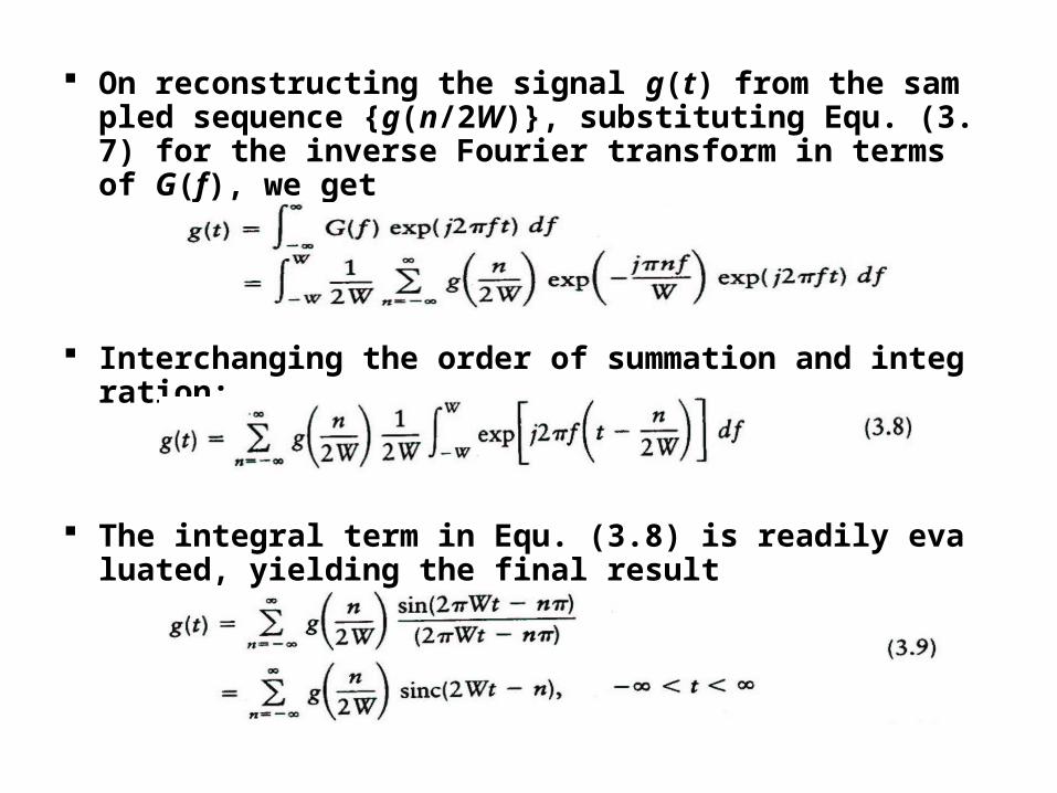
On reconstructing the signal g(t) from the sampled sequence {g(n/2W)}, substituting Equ. (3.7) for the inverse Fourier transform in terms of G(f), we get

Interchanging the order of summation and integration:

The integral term in Equ. (3.8) is readily evaluated, yielding the final result

Sampling theorem for band-limited signals of finite energy:

1). A band-limited signal of finite energy, which has no frequency components > W Hz, is completely described by the samples taken at instants of time separated by 1/2W seconds.

2). A band-limited signal of finite energy, which has no frequency components > W Hz, may be completely recovered from its samples taken at the rate of 2W samples/second.

The sampling rate of 2W samples/second, for a signal bandwidth of W Hertz, is called the Nyquist rate, and its reciprocal 1/2W seconds is called the Nyquist interval.

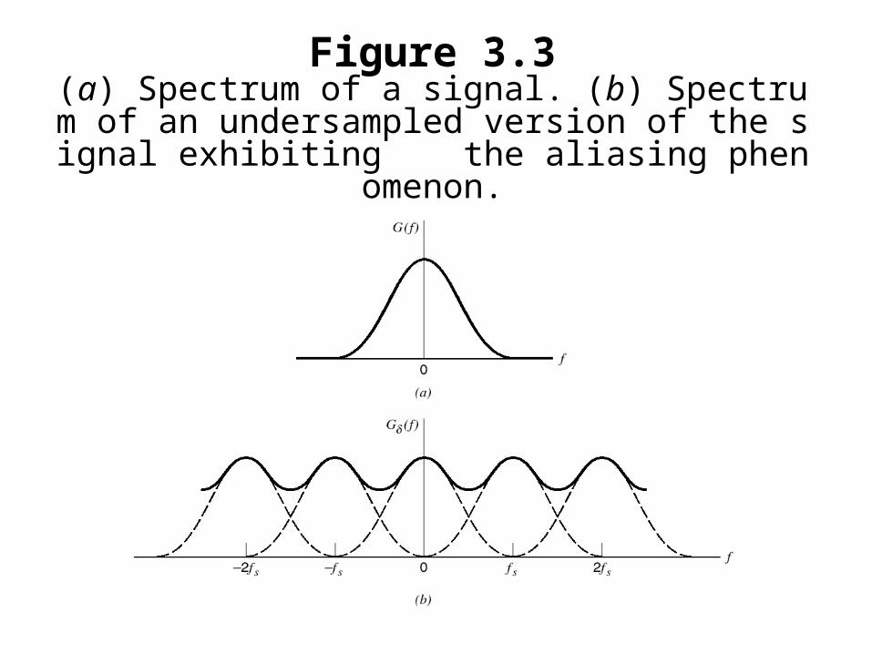
Figure 3.3(a) Spectrum of a signal. (b) Spectrum of an undersampled version of the signal exhibiting the alias

ing phenomenon.

The derivation of the sampling theorem is based on the

assumption that the signal g(t) is strictly band limited. In practice, an information-bearing signal is not strictly b

and limited, with some degree of under-sampling. Consequently, some aliasing is produced by the sampling process.

Two corrective measures for combating the aliasing effects :

1). Prior to sampling, an anti-aliasing LPF is used to attenuate those high-frequency components of the signal that are not essential to the information being conveyed by the signal.

2). The filtered signal is sampled at a rate slightly higher than the Nyquist rate.

Consider a message signal that has been anti-alias filtered,

resulting in the spectrum shown in Figure 3.4a.

The corresponding spectrum of the instantaneously sampled signal is shown in Figure 3.4b, assuming a sampling rate greater than the Nyquist rate.

The reconstruction filter may be specified (Figure 3.4c):

The reconstruction filter is LPF with a passband extending from -W to W, which is itself determined by the anti-aliasing filter.

The filter has a transition band extending from W to fs-W,

where fs is the sampling rate.

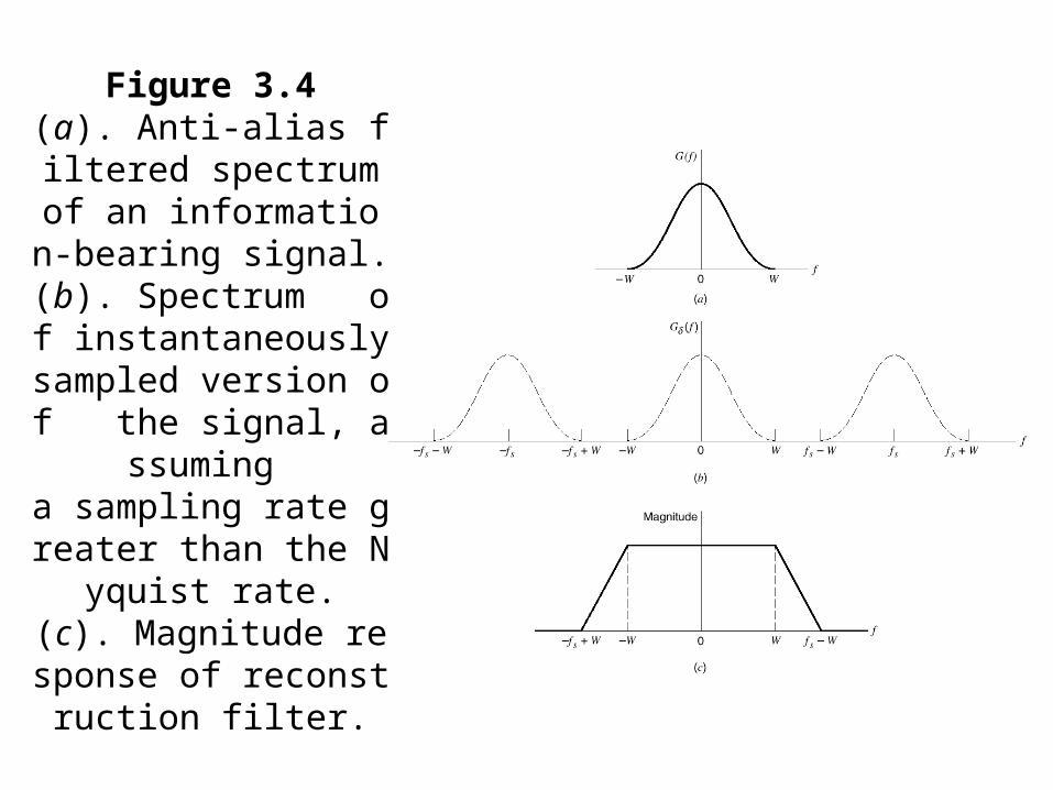
Figure 3.4(a). Anti-alias filtered spectrum of an information-bearing signal. (b).

Spectrum of instantaneously sampled version of the signal, assum

ing a sampling rate greater than the Nyquist rate.

(c). Magnitude response of reconstruction filter.

3.3 Pulse-Amplitude Modulation

The waveform of a PAM signal is illustrated in Figure 3.5.

The dashed curve depicts the waveform of a message signal m(t),

and the sequence of amplitude-modulated rectangular pulses shown

as solid lines represents the corresponding PAM signal s(t).

Two operations are involved in the generation of the PAM signal, these are jointly referred to as “sample and hold” :

1. Instantaneous sampling of the message signal m(t) every Ts sec,

where the sampling rate fs = 1/Ts is chosen with the sampling

theorem.

2. Lengthening the duration of each sample so obtained to some

constant value T.

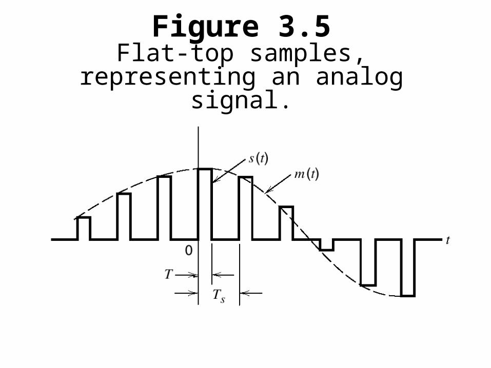
Figure 3.5Flat-top samples, representing an

analog signal.

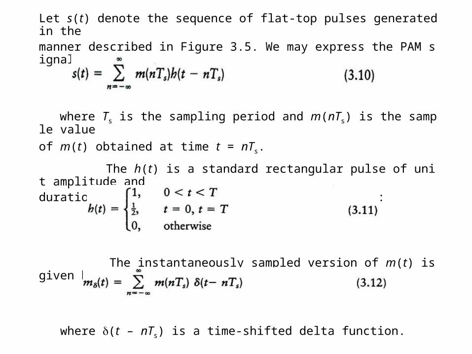
Let s(t) denote the sequence of flat-top pulses generated in themanner described in Figure 3.5. We may express the PAM signal as

where Ts is the sampling period and m(nTs) is the sample value

of m(t) obtained at time t = nTs.

The h(t) is a standard rectangular pulse of unit amplitude and duration T, defined as follows (see Figure 3.6a):

The instantaneously sampled version of m(t) is given by

where (t – nTs) is a time-shifted delta function.

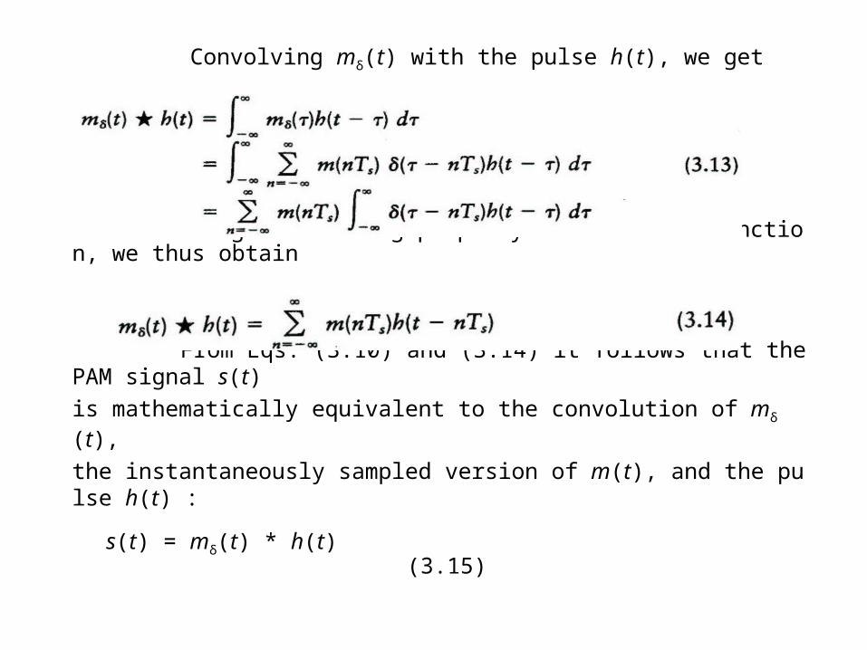
Convolving mδ(t) with the pulse h(t), we get

Using the sifting property of the delta function, we thus obtain

From Eqs. (3.10) and (3.14) it follows that the PAM signal s(t)

is mathematically equivalent to the convolution of mδ(t),

the instantaneously sampled version of m(t), and the pulse h(t) :

s(t) = mδ(t) * h(t) (3.15)

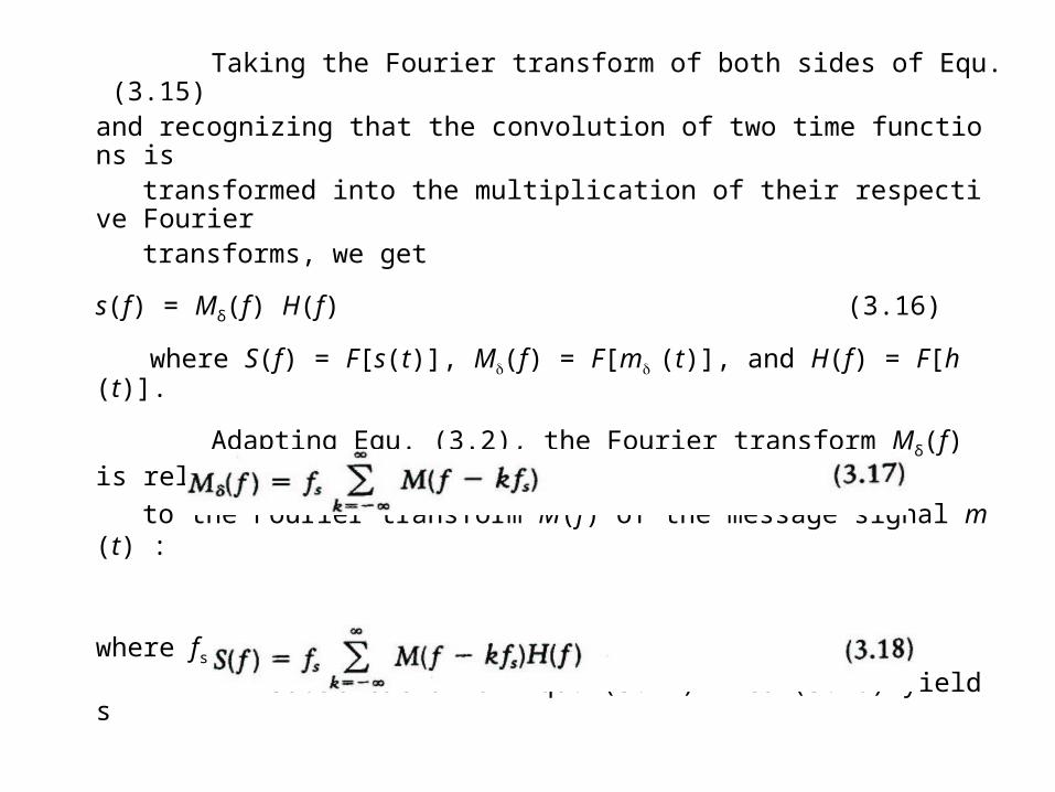
Taking the Fourier transform of both sides of Equ. (3.15) and recognizing that the convolution of two time functions is

transformed into the multiplication of their respective Fourier transforms, we get

s(f) = Mδ(f) H(f) (3.16)

where S(f) = F[s(t)], M(f) = F[m (t)], and H(f) = F[h(t)].

Adapting Equ. (3.2), the Fourier transform Mδ(f) is related

to the Fourier transform M(f) of the message signal m(t) :

where fs is the sampling rate. Substitution of Equ. (3.17) into (3.16) yields

To recover the original message m(t) from a PAM signal s(t),

we pass s(t) through a LPF with frequency response of Figure 3.4c;

here it is assumed that the message is limited to bandwidth W and

the sampling rate fs is > the Nyquist rate 2W.

From Equ. (3.18), the filter output spectrum is M(f)H(f).

This output is equivalent to passing the message signal m(t)

through another LPF of frequency response H(f).

From Equ. (3.11), the Fourier transform of the rectangular

pulse h(t) is as that plotted in Figure 3.6b:

H(f) = T sinc(fT) exp( － jfT) (3.19)

By using flat-top samples to generate a PAM signal,

we have introduced amplitude distortion as well as a delay of T/2.

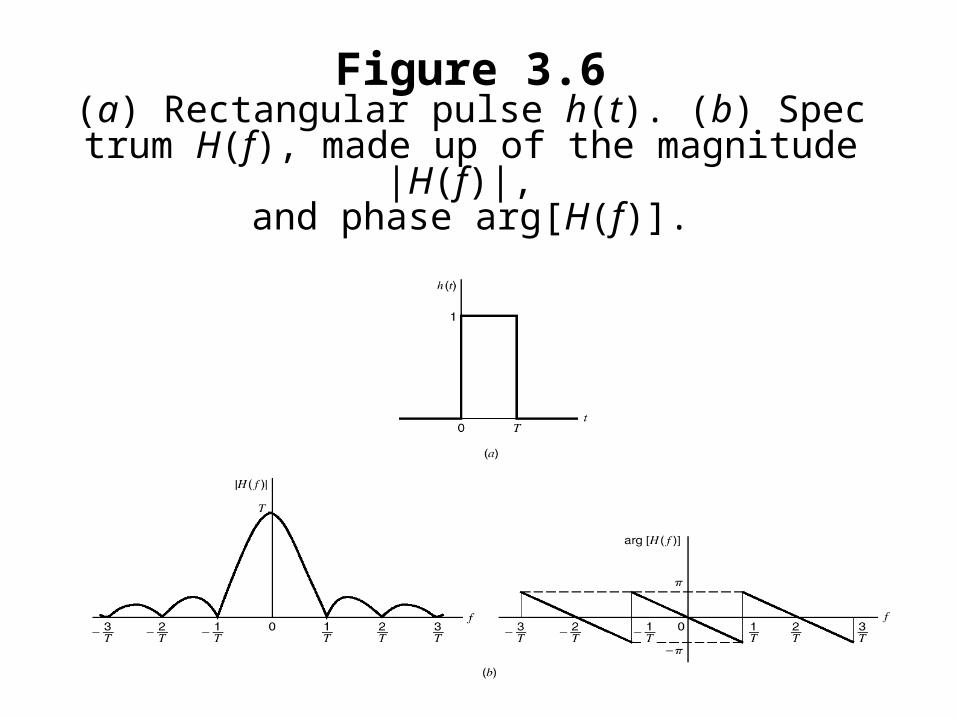
Figure 3.6(a) Rectangular pulse h(t). (b) Spectrum H(f), m

ade up of the magnitude |H(f)|, and phase arg[H(f)].

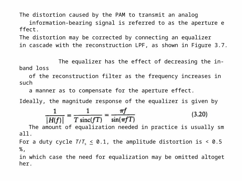
The distortion caused by the PAM to transmit an analog

information-bearing signal is referred to as the aperture effect.

The distortion may be corrected by connecting an equalizer

in cascade with the reconstruction LPF, as shown in Figure 3.7.

The equalizer has the effect of decreasing the in-band loss

of the reconstruction filter as the frequency increases in such

a manner as to compensate for the aperture effect.

Ideally, the magnitude response of the equalizer is given by

The amount of equalization needed in practice is usually small.

For a duty cycle T/Ts < 0.1, the amplitude distortion is < 0.5 %,

in which case the need for equalization may be omitted altogether.

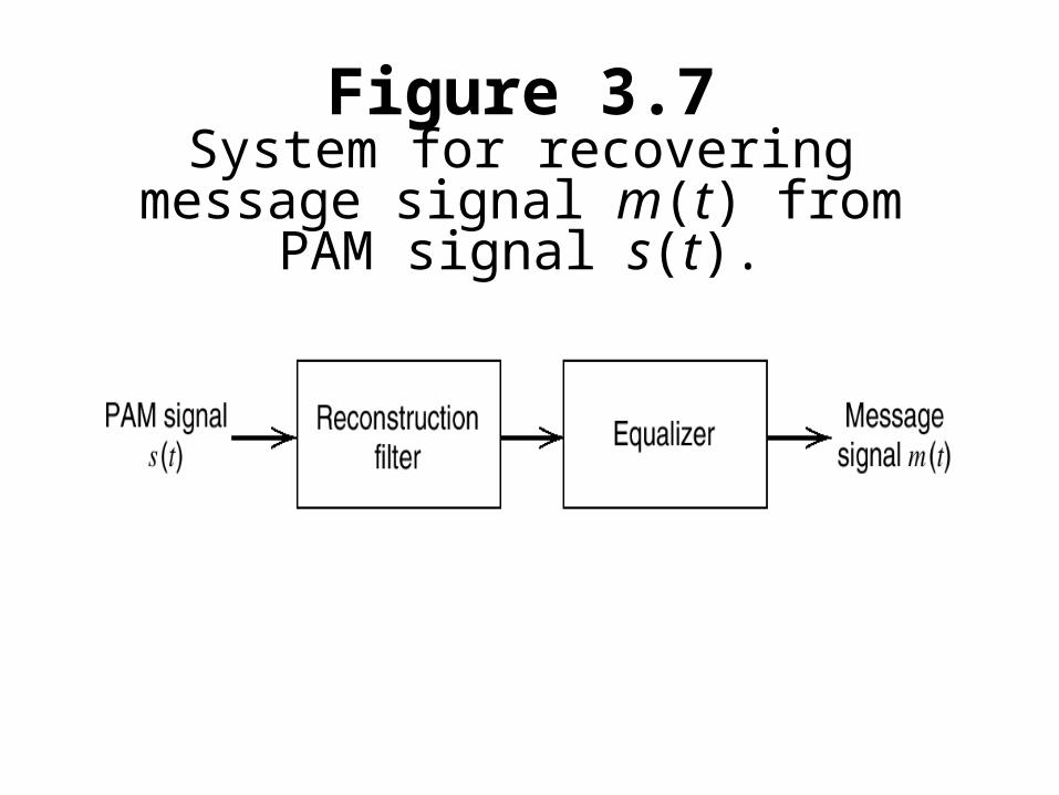
Figure 3.7System for recovering message signal m(t) from PAM signal s(t).

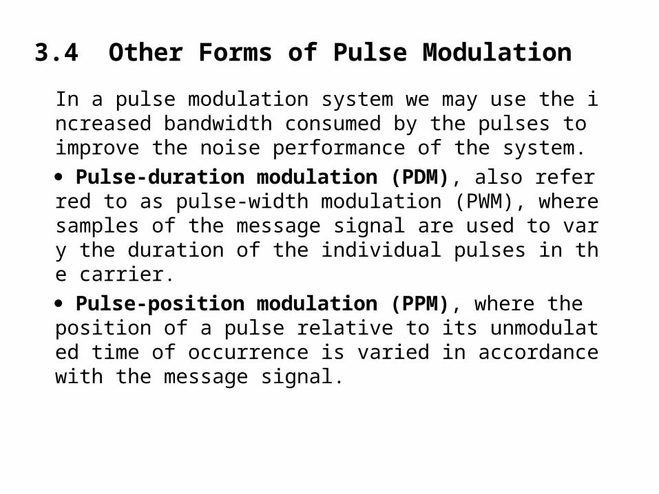
3.4 Other Forms of Pulse Modulation

In a pulse modulation system we may use the increased bandwidth consumed by the pulses to improve the noise performance of the system.

Pulse-duration modulation (PDM), also referred to as pulse-width modulation (PWM), where samples of the message signal are used to vary the duration of the individual pulses in the carrier.

Pulse-position modulation (PPM), where the position of a pulse relative to its unmodulated time of occurrence is varied in accordance with the message signal.

In PDM, long pulses expend considerable power while bearing no additional information. If this unused power is subtracted from PDM so that only time transitions are preserved, we obtain PPM.

Accordingly, PPM is a more efficient form of pulse modulation than PDM.

In a PPM system the transmitted information is contained in the relative positions of the modulated pulses, the presence of additive noise affects the performance of such a system by falsifying the time at which the modulated pulses are judged to occur.

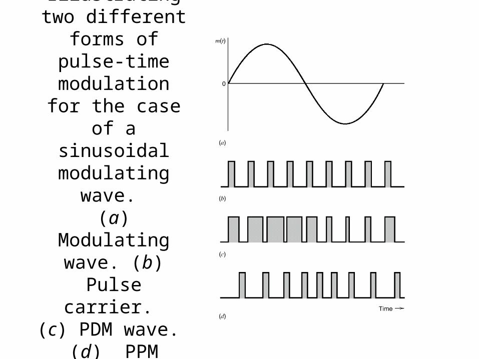
Figure 3.8Illustrating two

different forms of pulse-time

modulation for the case of a sinusoidal

modulating wave. (a) Modulating wave. (b) Pulse

carrier. (c) PDM wave. (d) PPM wave.

3.5 Bandwidth-Noise Trade-Off

PPM system is the optimum form of analog pulse modulation. Noise analysis of a PPM system reveals that PPM and FM systems exhibit a similar noise performance:

1. Both systems have a figure of merit proportional to the square of the transmission bandwidth normalized with respect to the message bandwidth.

2. Both systems exhibit a threshold effect as the SNR is reduced.

The practical implication of point 1 is that, in terms of a trade-off of increased transmission bandwidth for improved noise performance, the best way with CW modulation and analog pulse modulation systems is to follow a square law.

Two fundamental processes are involved in the generation of a binary PCM wave: sampling and quantization.

The sampling process takes care of the discrete-time representation of the message signal.

The quantization process takes care of the discrete-amplitude representation of the message signal.

The combined use of sampling and quantization permits the transmission of a message signal in coded form.

3.6 Quantization Process

Amplitude quantization is defined as the process of transforming

the sample amplitude m(nTs) of a message signal m(t) at time t = nTs into discrete amplitude v(nTs) taken from a finite set of possible amplitudes.

Assume the quantization process is memoryless and instantaneous,

which means that the transformation at time t = nTs is not affected by earlier or later samples of the message signal.

When dealing with a memoryless quantizer, we may use

the symbol m in place of m(nTs), as indicated in Figure 3.9a. As shown in Figure 3.9b, the signal amplitude m is specified by the index k if it lies inside the partition cell

k : {mk < m < mk+1}, k = 1, 2,..., L (3.21)

where L is the total number of amplitude levels used in the quantizer.

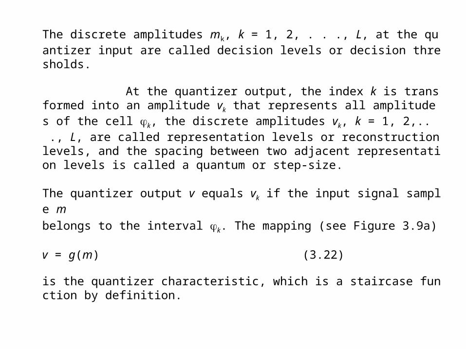
The discrete amplitudes mk, k = 1, 2, . . ., L, at the quantizer input are called decision levels or decision thresholds.

At the quantizer output, the index k is transformed into an amplitude vk that represents all amplitudes of the cell k, the discrete amplitudes vk, k = 1, 2,.. ., L, are called representation levels or reconstruction levels, and the spacing between two adjacent representation levels is called a quantum or step-size.

The quantizer output v equals vk if the input signal sample m

belongs to the interval k. The mapping (see Figure 3.9a)

v = g(m) (3.22)

is the quantizer characteristic, which is a staircase function by definition.

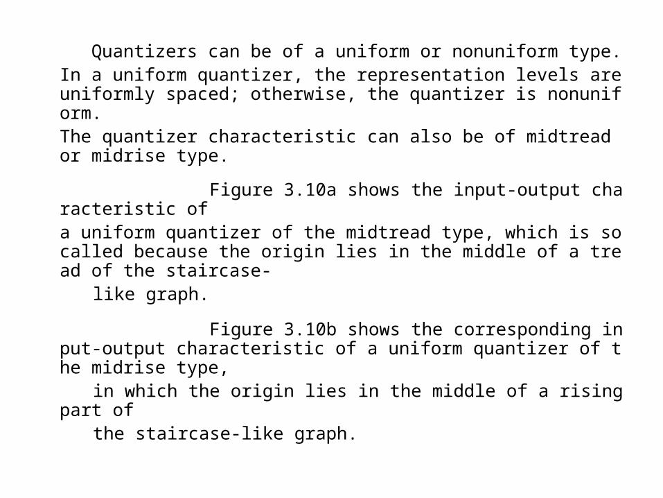
Quantizers can be of a uniform or nonuniform type. In a uniform quantizer, the representation levels are uniformly spaced; otherwise, the quantizer is nonuniform. The quantizer characteristic can also be of midtread or midrise type.

Figure 3.10a shows the input-output characteristic of a uniform quantizer of the midtread type, which is so called because the origin lies in the middle of a tread of the staircase-

like graph.

Figure 3.10b shows the corresponding input-output characteristic of a uniform quantizer of the midrise type,

in which the origin lies in the middle of a rising part of the staircase-like graph.

Figure 3.9Description of a memoryless quantizer.

Figure 3.10Two types of quantization: (a) midtread and (b)

midrise.

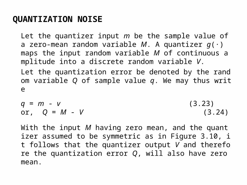
QUANTIZATION NOISE

Let the quantizer input m be the sample value of a zero-mean random variable M. A quantizer g(·) maps the input random variable M of continuous amplitude into a discrete random variable V.

Let the quantization error be denoted by the random variable Q of sample value q. We may thus write

q = m - v (3.23)or, Q = M - V (3.24)

With the input M having zero mean, and the quantizer assumed to be symmetric as in Figure 3.10, it follows that the quantizer output V and therefore the quantization error Q, will also have zero mean.

Consider an input m of continuous amplitude in the range (-mmax, mmax).

Assuming a uniform quantizer of the midrise type illustrated in Figure 3.10b, the step-size of the quantizer is given by

= 2mmax /L (3.25)

where L is the total number of representation levels.

For a uniform quantizer, the quantization error Q will have its sample values bounded by － /2 < q < /2.

If the step-size is sufficiently small (i.e., the number of representation levels L is sufficiently large), it is reasonable to assume that the quantization error Q is a uniformly distributed random variable.

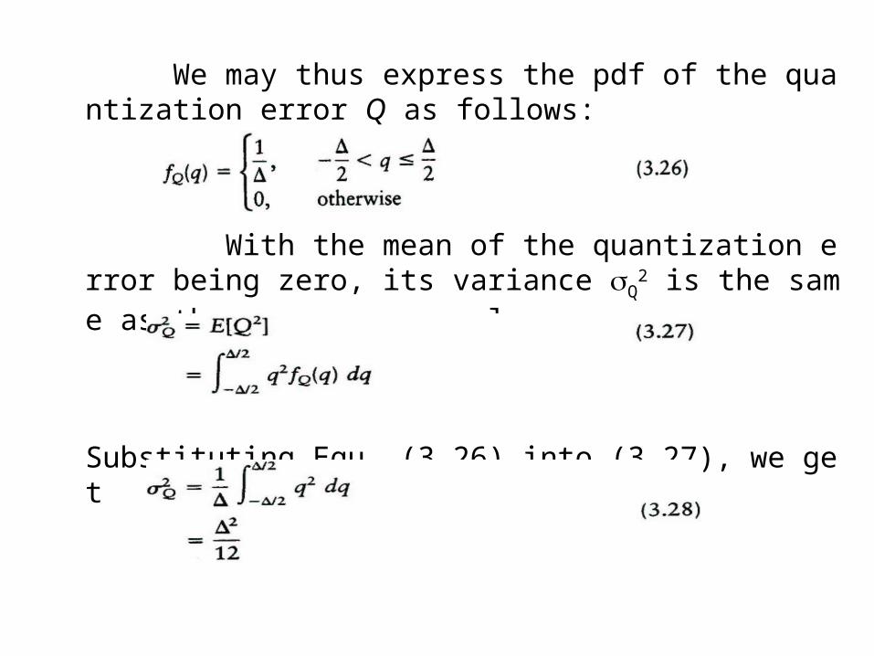
We may thus express the pdf of the quantization error Q as follows:

With the mean of the quantization error being zero, its variance Q

2 is the same as the mean-square value:

Substituting Equ. (3.26) into (3.27), we get

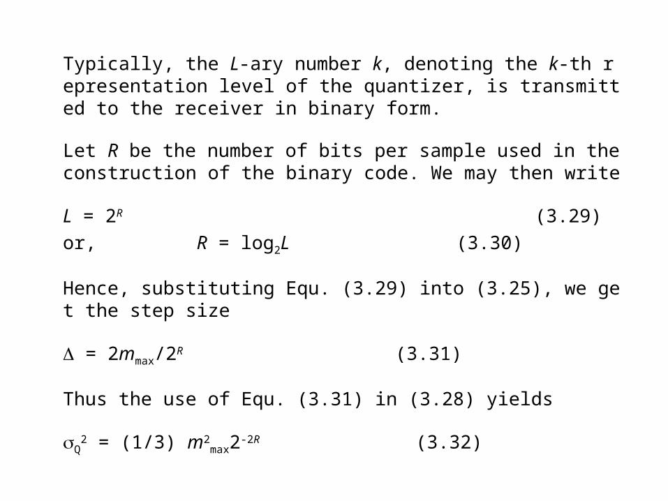
Typically, the L-ary number k, denoting the k-th representation level of the quantizer, is transmitted to the receiver in binary form.

Let R be the number of bits per sample used in the construction of the binary code. We may then write

L = 2R (3.29)

or, R = log2L (3.30)

Hence, substituting Equ. (3.29) into (3.25), we get the step size

= 2mmax/2R (3.31)

Thus the use of Equ. (3.31) in (3.28) yields

Q2 = (1/3) m2

max2-2R (3.32)

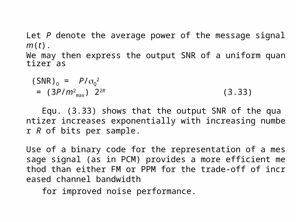
Let P denote the average power of the message signal m(t). We may then express the output SNR of a uniform quantizer as

(SNR)O = P/Q2

= (3P/m2max) 22R (3.33)

Equ. (3.33) shows that the output SNR of the quantizer increases exponentially with increasing number R of bits per sample.

Use of a binary code for the representation of a message signal (as in PCM) provides a more efficient method than either FM or PPM for the trade-off of increased channel bandwidth

for improved noise performance.

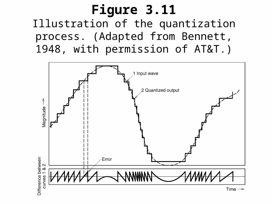
Figure 3.11Illustration of the quantization process.

(Adapted from Bennett, 1948, with permission of AT&T.)

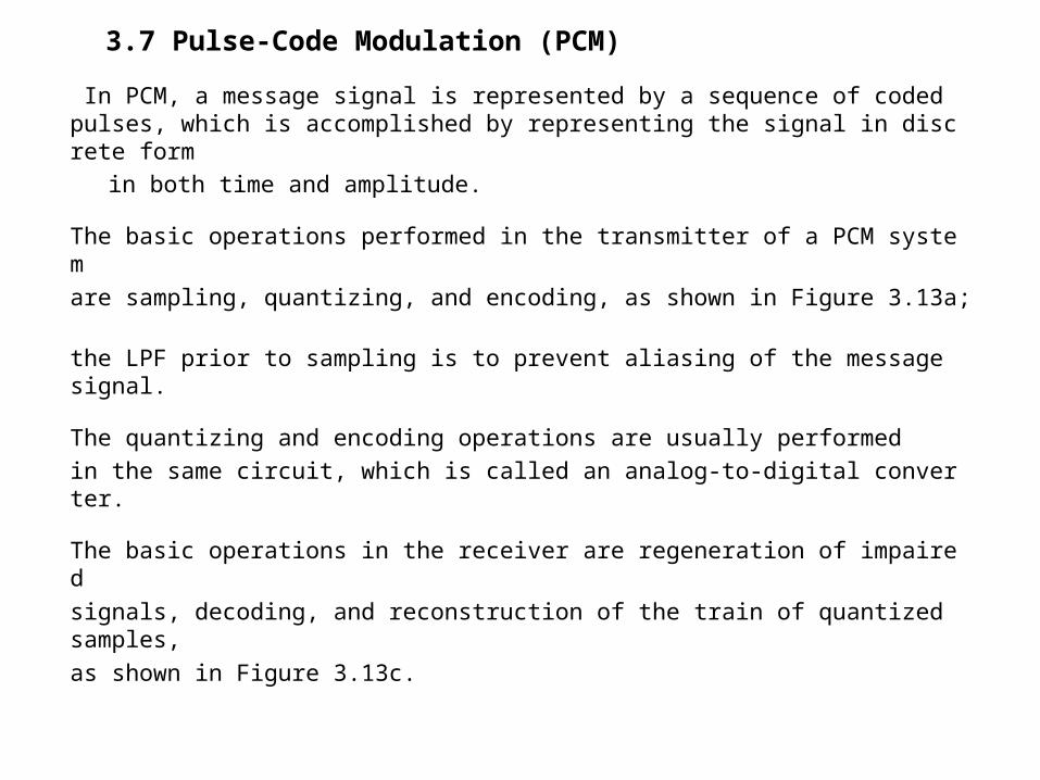
3.7 Pulse-Code Modulation (PCM)

In PCM, a message signal is represented by a sequence of coded pulses, which is accomplished by representing the signal in discrete form

in both time and amplitude.

The basic operations performed in the transmitter of a PCM system

are sampling, quantizing, and encoding, as shown in Figure 3.13a;

the LPF prior to sampling is to prevent aliasing of the message signal.

The quantizing and encoding operations are usually performed

in the same circuit, which is called an analog-to-digital converter.

The basic operations in the receiver are regeneration of impaired

signals, decoding, and reconstruction of the train of quantized samples,

as shown in Figure 3.13c.

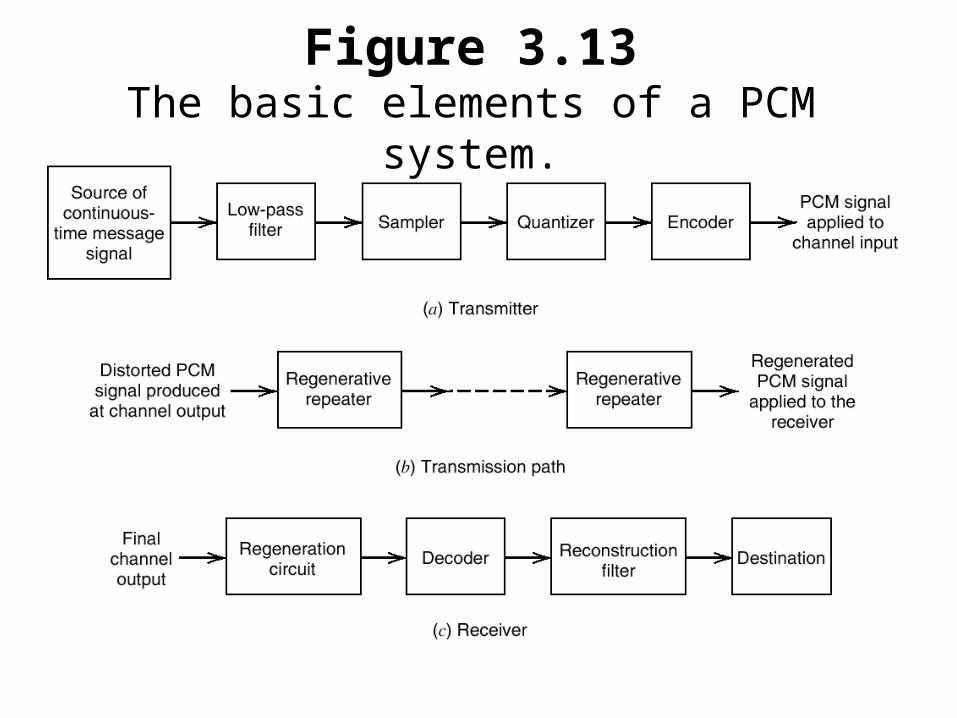
Figure 3.13The basic elements of a PCM system.

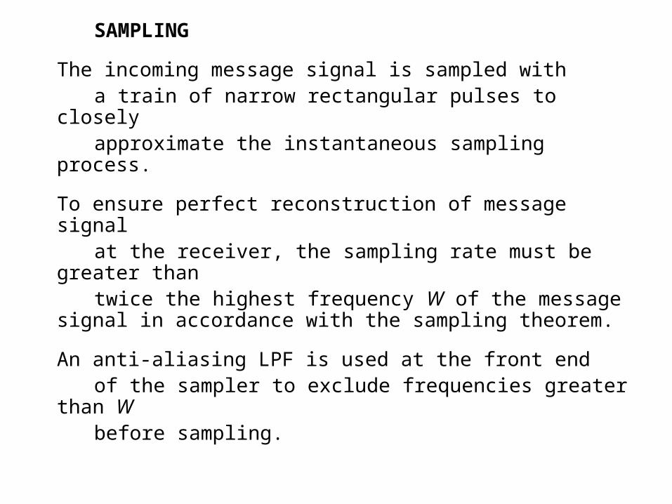
SAMPLING

The incoming message signal is sampled with a train of narrow rectangular pulses to closely approximate the instantaneous sampling process.

To ensure perfect reconstruction of message signal at the receiver, the sampling rate must be greater than twice the highest frequency W of the message signal in

accordance with the sampling theorem.

An anti-aliasing LPF is used at the front end of the sampler to exclude frequencies greater than W before sampling.

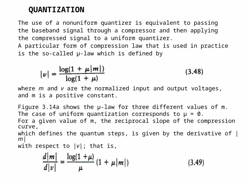
QUANTIZATION

The use of a nonuniform quantizer is equivalent to passing the baseband signal through a compressor and then applying the compressed signal to a uniform quantizer.

A particular form of compression law that is used in practice is the so-called μ-law which is defined by

where m and v are the normalized input and output voltages, and m is a positive constant.

Figure 3.14a shows the μ-law for three different values of m. The case of uniform quantization corresponds to μ = 0. For a given value of m, the reciprocal slope of the compression curve, which defines the quantum steps, is given by the derivative of |m| with respect to |v|; that is,

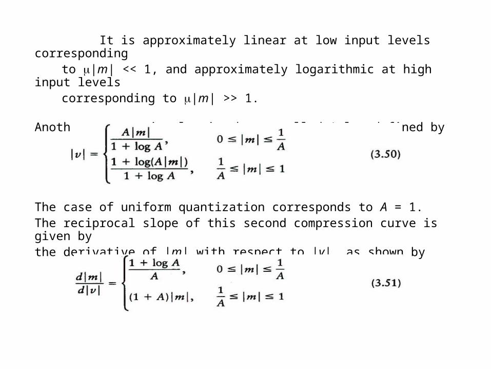
It is approximately linear at low input levels corresponding to |m| << 1, and approximately logarithmic at high input levels corresponding to |m| >> 1.

Another compression law is the so-called A-law defined by

The case of uniform quantization corresponds to A = 1. The reciprocal slope of this second compression curve is given by the derivative of |m| with respect to |v|, as shown by

To restore the signal samples to their correct relative level,

we must use a device in the receiver with a characteristic complementary

to the compressor. Such a device is called an expander.

The compression and expansion laws are ideally inverse

so that the expander output is equal to the compressor input.

The combination of a compressor and an expander is called

a compander.

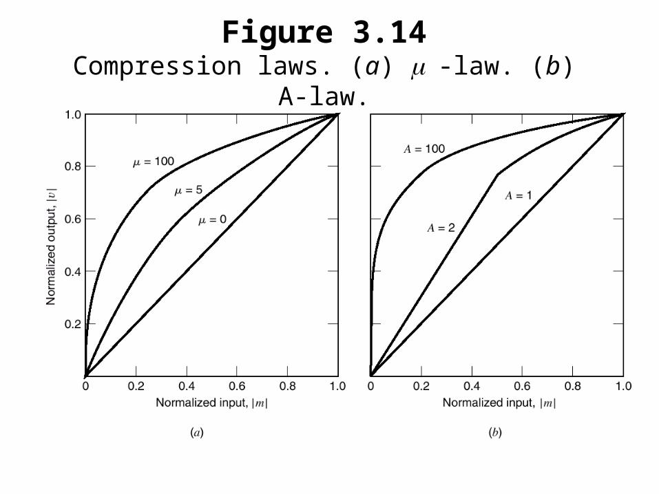
Figure 3.14Compression laws. (a) -law. (b) A-law.

ENCODINGTo exploit the advantages of sampling and quantizing for making

the transmitted signal more robust to noise, interference and other

channel impairments, an encoding process is required to translate

the discrete set of sample values to a more appropriate form of signal.

Any plan for representing each of this discrete set of values

as a particular arrangement of discrete events is called a code.

One of the discrete events in a code is called a code element or symbol.

A particular arrangement of symbols used in a code to represent

a single value of the discrete set is called a code word or character.

The maximum advantage over the effects of noise in a transmission medium is obtained by using a binary code, because a binary symbol withstands a relatively high level of noise and is easy to regenerate.

Suppose that, in a binary code, each code word consists of R bits,

thus R denotes the number of bits per sample. Using such a code,

we may represent a total of 2R distinct numbers.

3.8 Noise Consideration in PCM Systems

PCM system performance is influenced by two major noise sources:

1). Channel noise, which is introduced anywhere between

the transmitter output and the receiver input.

2). Quantization noise, which is introduced in the transmitter and

is carried all the way along to the receiver output.

The main effect of channel noise is to introduce bit errors into

the received signal. In the case of a binary PCM system, the presence

of a bit error causes symbol 1 to be mistaken for symbol 0, or vice versa.

The fidelity of information transmission by PCM in the presence

of channel noise may be measured in terms of the average probability of

symbol error, which is defined as the probability that the reconstructed symbol at the receiver output differs from the transmitted binary symbol,

on the average.

The average probability of symbol error, also referred to as the bit error rate (BER), assumes that all the bits in the original binary wave are of equal importance.

To optimize system performance in the presence of channel noise, we need to minimize the average probability of symbol error.

For this evaluation, it is customary to model the channel noise as additive, white, and Gaussian.

The effect of channel noise can be made practically negligible by ensuring an adequate signal-energy to noise-density ratio through the provision of short-enough spacing between regenerative repeaters in the PCM system.

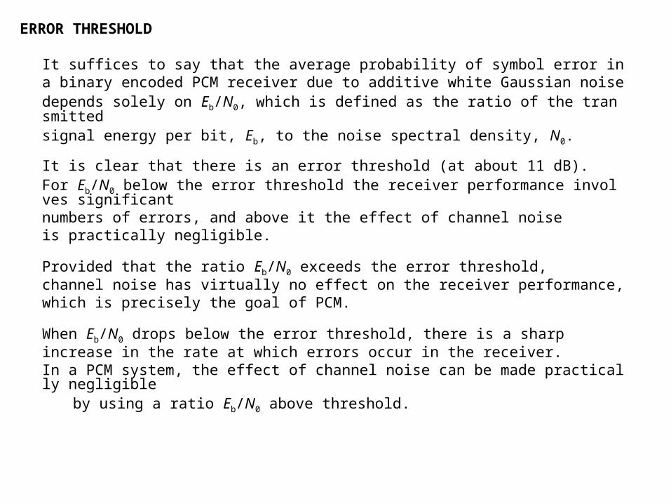
ERROR THRESHOLD

It suffices to say that the average probability of symbol error in a binary encoded PCM receiver due to additive white Gaussian noise depends solely on Eb/N0, which is defined as the ratio of the transmitted signal energy per bit, Eb, to the noise spectral density, N0.

It is clear that there is an error threshold (at about 11 dB). For Eb/N0 below the error threshold the receiver performance involves significantnumbers of errors, and above it the effect of channel noise is practically negligible.

Provided that the ratio Eb/N0 exceeds the error threshold, channel noise has virtually no effect on the receiver performance, which is precisely the goal of PCM.

When Eb/N0 drops below the error threshold, there is a sharp increase in the rate at which errors occur in the receiver. In a PCM system, the effect of channel noise can be made practically negligible

by using a ratio Eb/N0 above threshold.

3.9 Time-Division Multiplexing The sampling theorem provides the basis for transmitting

the information contained in a band-limited message signal m(t) as a sequence of samples of m(t) taken uniformly at a rate that is usually slightly higher than the Nyquist rate.

A time-division multiplex (TDM) system enables the joint utilizationof a common communication channel by a plurality of independent message

sources without mutual interference among them. Each input message signal is first restricted in bandwidth by an

anti-aliasing LPF to remove the frequencies that are nonessential to an adequate signal representation.

The LPF outputs are then applied to a commutator, which is usually implemented using electronic switching circuitry.

The function of the commutator is twofold: (1) To take a narrow sample of each of the N input messages at a rate fs that is slightly > 2W, where W is the cutoff frequency of the anti-aliasing filter; (2) To sequentially interleave these N samples inside the sampling interval Ts.

It is clear that the use of TDM introduces a bandwidth expansion factor N, because the scheme must squeeze N samples derived from N independentmessage sources into a time slot equal to one sampling interval.

At the receiving end of the system, the received signal is applied to a pulse demodulator, which performs the reverse operation of the pulse modulator.

The narrow samples produced at the pulse demodulator output are distributed to the appropriate low-pass reconstruction filters by means of a decommutator, which operates in synchronism with the commutator in the transmitter.

The TDM system is highly sensitive to dispersion in the common channel, that is, to variations of amplitude with frequency or lack of proportionality of phase with frequency.

Accordingly, accurate equalization of both magnitude and phase responses of the channel is necessary to ensure a satisfactory operation of the system.

Unlike FDM, to a first-order approximation TDM is immune to nonlinearities in the channel as a source of cross-talk.

The reason for this behavior is that different message signals are not simultaneously applied to the channel.

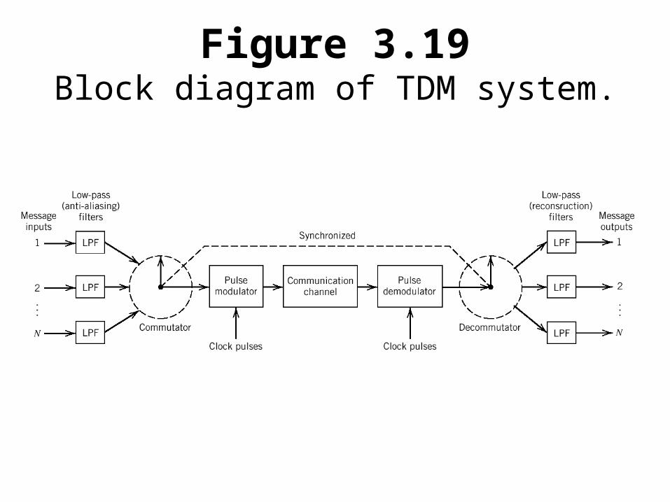
Figure 3.19Block diagram of TDM system.

3.10 Digital Multiplexers

The multiplexing of digital signals is accomplished by using a bit-by-bit interleaving procedure with a selector switch that sequentially takesa bit from each incoming line and then applies it to the high-speed common line.

At the receiving end of the system the output of this common line is separated out into its low-speed individual components and then delivered to their respective destinations.

Digital multiplexers are categorized into two major groups. One group of multiplexers is used to take relatively low bit-rate data streams

originating from digital computers and multiplex them for TDM transmission over the public switched telephone network.

The second group of digital multiplexers forms part of the data transmission service provided by telecommunication carriers such as AT&T.

A worldwide feature of the hierarchy is that it starts at 64 kb/s, which corresponds to the standard PCM representation of a voice signal. An incoming bit stream at this rate, is called a digital signal zero (DS0).

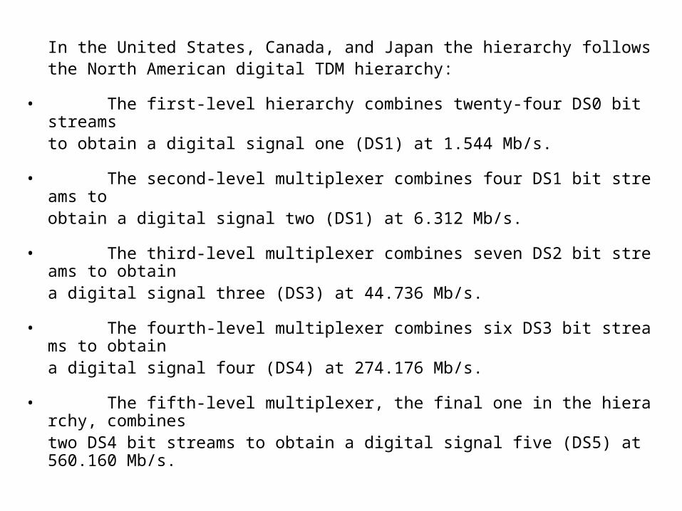
In the United States, Canada, and Japan the hierarchy follows the North American digital TDM hierarchy:

• The first-level hierarchy combines twenty-four DS0 bit streams to obtain a digital signal one (DS1) at 1.544 Mb/s.

• The second-level multiplexer combines four DS1 bit streams to obtain a digital signal two (DS1) at 6.312 Mb/s.

• The third-level multiplexer combines seven DS2 bit streams to obtain a digital signal three (DS3) at 44.736 Mb/s.

• The fourth-level multiplexer combines six DS3 bit streams to obtain a digital signal four (DS4) at 274.176 Mb/s.

• The fifth-level multiplexer, the final one in the hierarchy, combines two DS4 bit streams to obtain a digital signal five (DS5) at 560.160 M

b/s.

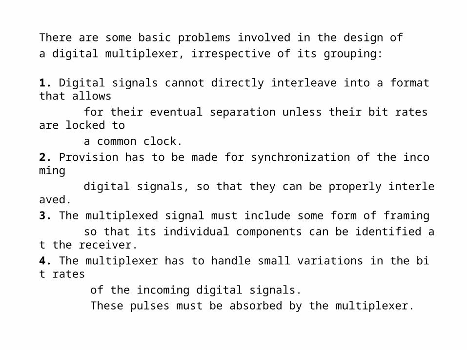
There are some basic problems involved in the design of

a digital multiplexer, irrespective of its grouping:

1. Digital signals cannot directly interleave into a format that allows

for their eventual separation unless their bit rates are locked to

a common clock.

2. Provision has to be made for synchronization of the incoming

digital signals, so that they can be properly interleaved.

3. The multiplexed signal must include some form of framing

so that its individual components can be identified at the receiver.

4. The multiplexer has to handle small variations in the bit rates

of the incoming digital signals.

These pulses must be absorbed by the multiplexer.

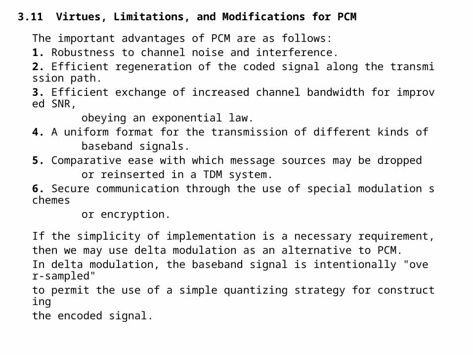
3.11 Virtues, Limitations, and Modifications for PCM

The important advantages of PCM are as follows: 1. Robustness to channel noise and interference. 2. Efficient regeneration of the coded signal along the transmission path. 3. Efficient exchange of increased channel bandwidth for improved SNR,

obeying an exponential law. 4. A uniform format for the transmission of different kinds of

baseband signals. 5. Comparative ease with which message sources may be dropped

or reinserted in a TDM system. 6. Secure communication through the use of special modulation schemes

or encryption.

If the simplicity of implementation is a necessary requirement, then we may use delta modulation as an alternative to PCM. In delta modulation, the baseband signal is intentionally "over-sampled" to permit the use of a simple quantizing strategy for constructing the encoded signal.

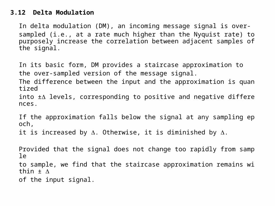
3.12 Delta Modulation

In delta modulation (DM), an incoming message signal is over-sampled (i.e., at a rate much higher than the Nyquist rate) to purposely increase the correlation between adjacent samples of the signal.

In its basic form, DM provides a staircase approximation to the over-sampled version of the message signal. The difference between the input and the approximation is quantized into ± levels, corresponding to positive and negative differences.

If the approximation falls below the signal at any sampling epoch, it is increased by . Otherwise, it is diminished by .

Provided that the signal does not change too rapidly from sample to sample, we find that the staircase approximation remains within ± of the input signal.

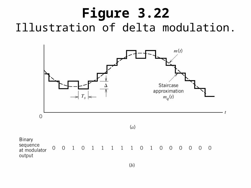
Figure 3.22Illustration of delta modulation.

Let m(t) denote the input (message) signal, and mq(t) denote its staircase approximation. We adopt the following notation that is commonly used in the digital signal processing literature:

m[n] = m(nTs), n = 0, ±l, ±2, . . .

where Ts is the sampling period and m(nTs) is a sample of the signal m(t) taken at t = nTs and likewise for the samples of other continuous-time signals.

We may then formalize the basic principles of delta modulation in the following set of discrete-time relations:

e[n] = m[n] － mq[n – 1] (3.52)eq = Δ sgn(e[n]) (3.53)mq[n] = mq[n – 1] + eq[n] (3.54)

where e[n] is an error signal representing the difference between the present sample m[n] of the input signal and the latest approximation mq[n – 1] to it, eq[n] is the quantized version of e[n], and sgn(·) is the signum function. The quantizer output mq[n] is coded to produce the DM signal.

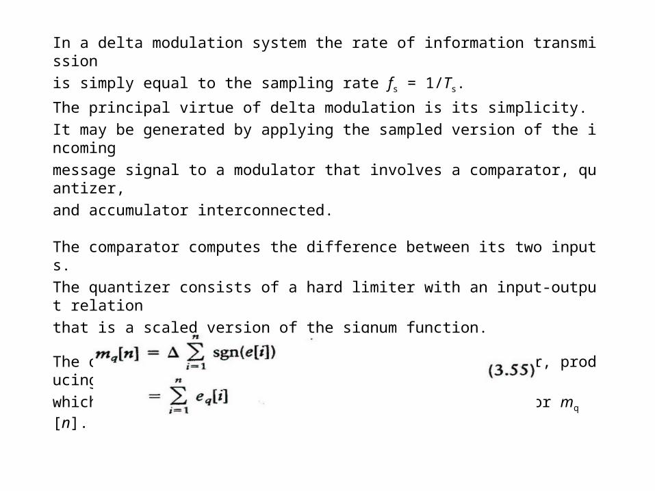
In a delta modulation system the rate of information transmission

is simply equal to the sampling rate fs = 1/Ts.

The principal virtue of delta modulation is its simplicity.

It may be generated by applying the sampled version of the incoming

message signal to a modulator that involves a comparator, quantizer,

and accumulator interconnected.

The comparator computes the difference between its two inputs.

The quantizer consists of a hard limiter with an input-output relation

that is a scaled version of the signum function.

The quantizer output is then applied to an accumulator, producing

which is obtained by solving Eqs. (3.53) and (3.54) for mq[n].

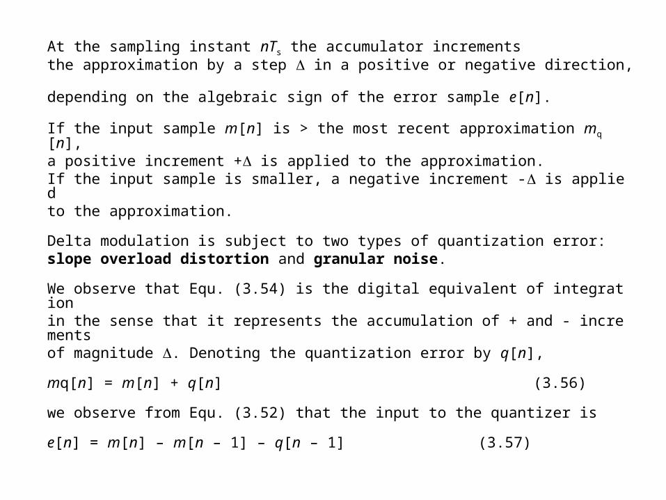
At the sampling instant nTs the accumulator increments the approximation by a step in a positive or negative direction, depending on the algebraic sign of the error sample e[n].

If the input sample m[n] is > the most recent approximation mq[n], a positive increment + is applied to the approximation.

If the input sample is smaller, a negative increment - is applied to the approximation.

Delta modulation is subject to two types of quantization error: slope overload distortion and granular noise.

We observe that Equ. (3.54) is the digital equivalent of integration in the sense that it represents the accumulation of + and - increments of magnitude . Denoting the quantization error by q[n],

mq[n] = m[n] + q[n] (3.56)

we observe from Equ. (3.52) that the input to the quantizer is

e[n] = m[n] – m[n – 1] – q[n – 1] (3.57)

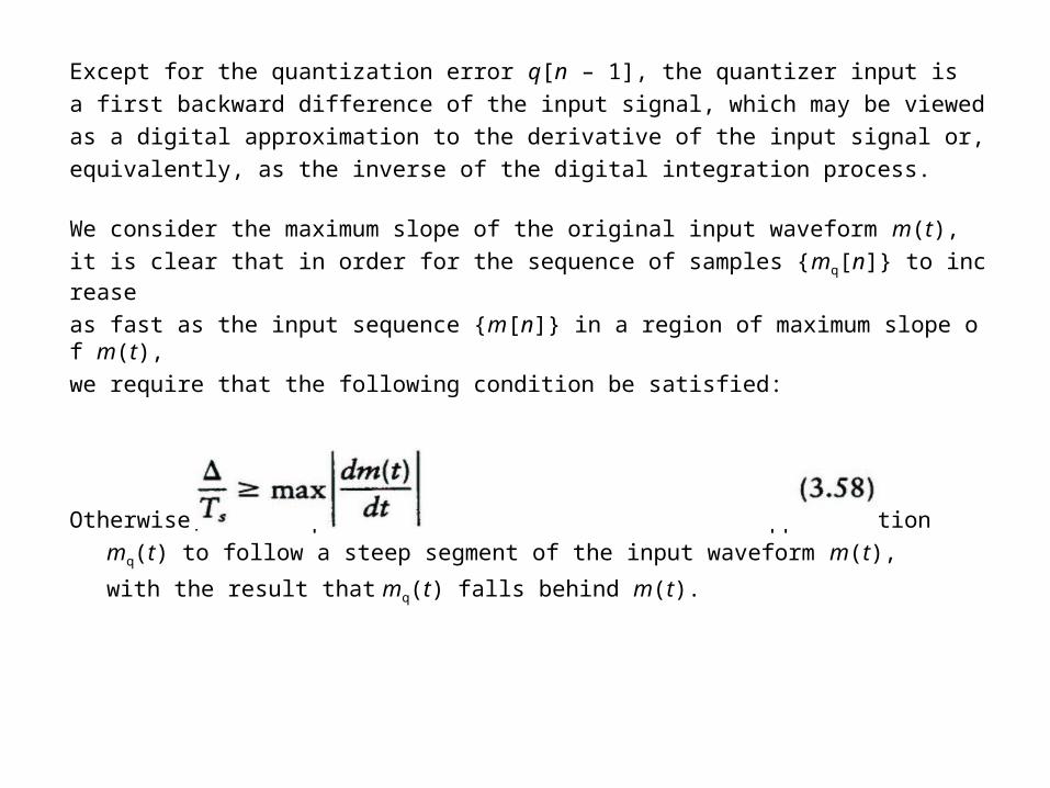
Except for the quantization error q[n – 1], the quantizer input is

a first backward difference of the input signal, which may be viewed

as a digital approximation to the derivative of the input signal or,

equivalently, as the inverse of the digital integration process.

We consider the maximum slope of the original input waveform m(t),

it is clear that in order for the sequence of samples {mq[n]} to increase

as fast as the input sequence {m[n]} in a region of maximum slope of m(t),

we require that the following condition be satisfied:

Otherwise, the step is too small for the staircase approximation

mq(t) to follow a steep segment of the input waveform m(t),

with the result that mq(t) falls behind m(t).

This condition is called slope overload, and the resulting quantization error is called slope-overload distortion (noise). A delta modulator using a fixed step size is often referred to as a linear delta modulator.

In contrast to slope-overload distortion, granular

noise occurs when the step size is too large relative to

the local slope characteristics of the input waveform m(t),

thereby causing the staircase approximation mq(t) to

hunt around a relatively flat segment of the input waveform.

Granular noise is analogous to quantization noise in

a PCM system.

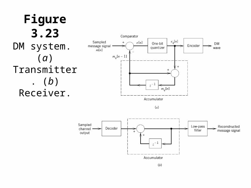
Figure 3.23DM system.

(a) Transmitter. (b) Receiver.

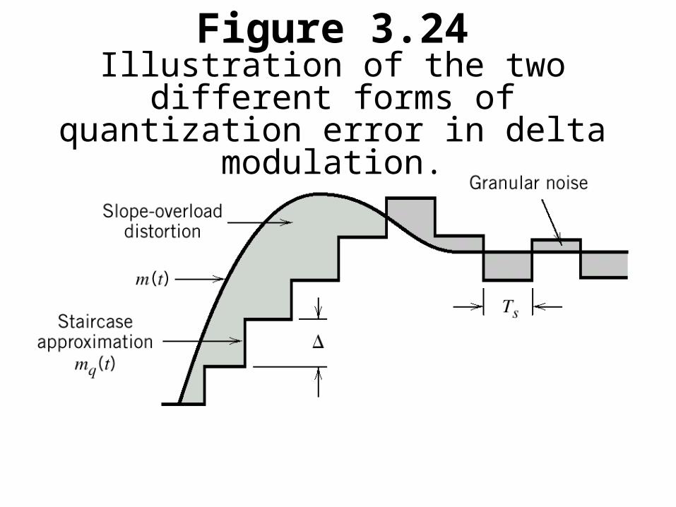
Figure 3.24Illustration of the two different forms

of quantization error in delta modulation.

3.13 Differential Pulse-Code Modulation

When a voice or video signal is sampled at a rate slightly higher than the Nyquist rate, the resulting sampled signal exhibits a high degree of correlation between adjacent samples.

When these highly correlated samples are encoded, as in PCM, the resulting encoded signal contains redundant information. By removing this redundancy before encoding, we obtain a more efficient coded signal, which is the basic idea behind DPCM.

Suppose then a baseband signal m(t) is sampled at the rate fs = 1/Ts

to produce the sequence {m[n]} whose samples are Ts seconds apart. In this scheme, the input signal to the quantizer is defined by

e[n] = m[n] – m^[n] (3.74)

which is the difference between the unquantized input sample m[n] and a prediction of it, denoted by m^[n].

The difference signal e[n] is the prediction error, since it is the amount by which the prediction filter fails to predict the input exactly. By encoding the quantizer output, we obtain a variant of PCM known as differential pulse-code modulation (DPCM).

The quantizer output may be expressed as

eq[n] = e[n] + q[n] (3.75)

where q[n] is the quantization error. The quantizer output eq[n] is added to the predicted value m^[n] to produce the prediction-filter input

mq[n] = m^[n] + eq[n] (3.76)

Substituting Equ. (3.75) into (3.76), we get

mq[n] = m^[n] + e[n] + q[n] (3.77)

From Equ. (3.74) we observe that the sum term m^[n] + e[n] is equal to the input sample m[n].

We may simplify Equ. (3.77) as

mq[n] = m[n] + q[n] (3.78)

which represents a quantized version of the input sample m[n].

If the prediction is good, the variance of the prediction error e[n]

will be smaller than the variance of m[n], so that a quantizer with

a given number of levels can be adjusted to produce a quantization error

with a smaller variance than would be possible if the input sample m[n]

were quantized directly as in a standard PCM system.

The receiver for reconstructing the quantized version of the input.

It consists of a decoder to reconstruct the quantized error signal.

The quantized version of the original input is reconstructed from

the decoder output using the same prediction filter used in the transmitter

of Figure 3.28a.

In the absence of channel noise, the encoded signal

at the receiver input is identical to the encoded signal

at the transmitter output.

Accordingly, the corresponding receiver output is equal to mq

[n], which differs from the original input m[n] only by

the quantization error q[n] incurred as a result of quantizing the prediction error e[n].

DPCM, like DM, is subject to slope-overload distortion whenever the input signal changes too rapidly

for the prediction filter to track it.

Also, like PCM, DPCM suffers from quantization noise.

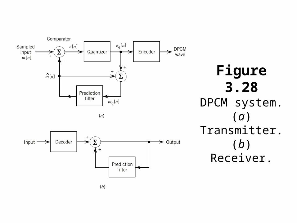
Figure 3.28DPCM system. (a) Transmitter.

(b) Receiver.