Chapter 22 Equilibrium Asset Pricing © 2014 OnCourse Learning. All Rights Reserved.1

© 2014 OnCourse Learning. All Rights Reserved. 1

Chapter 22

Equilibrium Asset Pricing


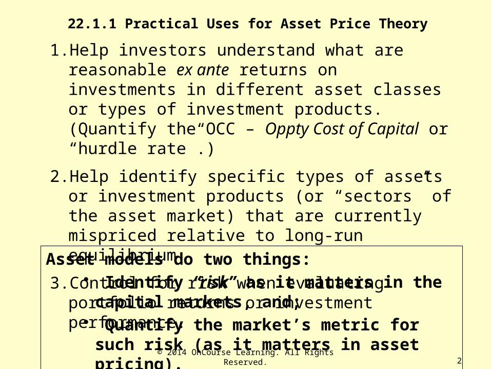
1. Help investors understand what are reasonable ex ante returns on investments in different asset classes or types of investment products. (Quantify the OCC – Oppty Cost of Capital or “hurdle rate”.)

2. Help identify specific types of assets or investment products (or “sectors” of the asset market) that are currently mispriced relative to long-run equilibrium.

3. Control for risk when evaluating portfolio returns or investment performance.

22.1.1 Practical Uses for Asset Price Theory

Asset models do two things:• Identify “risk” as it matters in the capital markets,

and;• Quantify the market’s metric for such risk (as it

matters in asset pricing).


The relationship between equilibrium asset price models and investment policy…

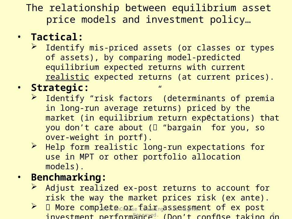
The relationship between equilibrium asset price models and investment policy…

• Tactical: Identify mis-priced assets (or classes or types of assets), by comparing

model-predicted equilibrium expected returns with current realistic expected returns (at current prices).

• Strategic: Identify “risk factors” (determinants of premia in long-run average

returns) priced by the market (in equilibrium return expectations) that you don’t care about ( “bargain” for you, so over-weight in portf).

Help form realistic long-run expectations for use in MPT or other portfolio allocation models).

• Benchmarking: Adjust realized ex-post returns to account for risk the way the market

prices risk (ex ante). More complete or fair assessment of ex post investment performance.

(Don’t confuse taking on more risk for “beating the market.”)



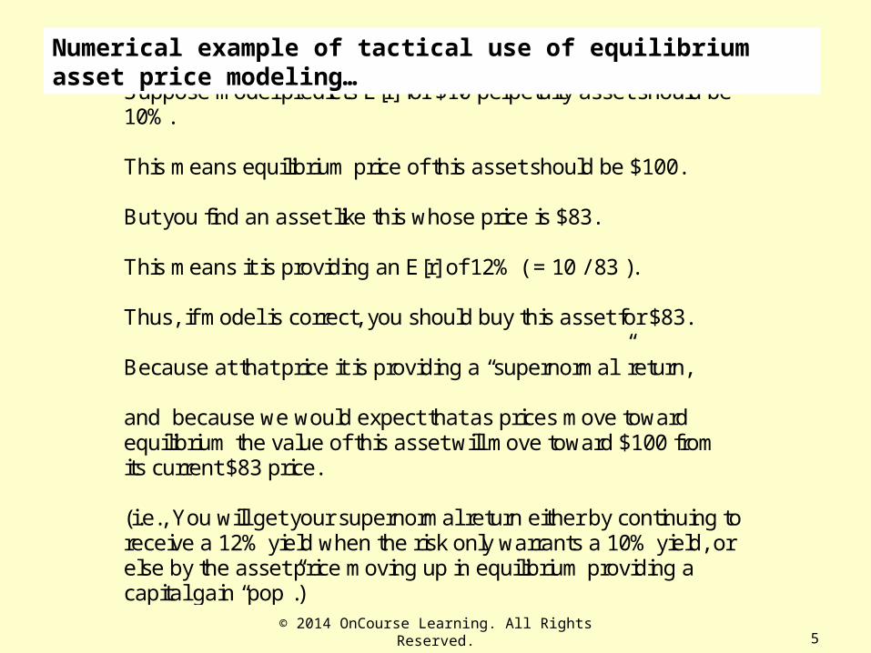
Quick & simple example… Suppose model predicts E[r] for $10 perpetuity asset should be 10%. This means equilibrium price of this asset should be $100. But you find an asset like this whose price is $83. This means it is providing an E[r] of 12% ( = 10 / 83 ). Thus, if model is correct, you should buy this asset for $83. Because at that price it is providing a “supernormal” return, and because we would expect that as prices move toward equilibrium the value of this asset will move toward $100 from its current $83 price. (i.e., You will get your supernormal return either by continuing to receive a 12% yield when the risk only warrants a 10% yield, or else by the asset price moving up in equilibrium providing a capital gain “pop”.)

Numerical example of tactical use of equilibrium asset price modeling…


22.1.2 A Threshold Point: What Underlies Asset Risk?

Most of the volatility in asset prices does not derive from rational changes in future cash flow expectations

Simulated Historical Present Values

Using VAR-Forecasted Cash Flows (CF) & Returns (R) in Present Value Model

0.8

0.9

1.0

1.1

1.2

1.3

1.4

1.5

1.6

1.7

1.8

1975 1976 1977 1978 1979 1980 1981 1982 1983 1984 1985 1986 1987 1988 1989 1990 1991 1992

Source: Geltner & Mei (1995)

Both CF & R Variable CF Constant, R Variable CF Variable, R Constant

Source: Geltner and Mei (1995).

7

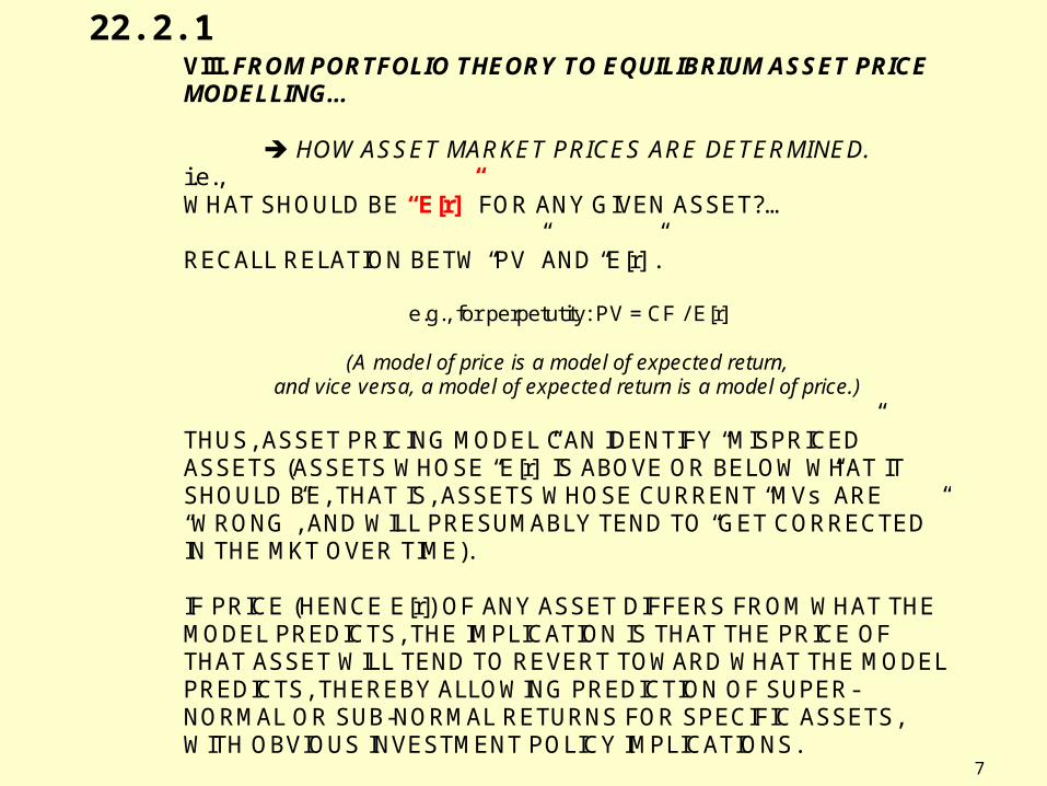
VIII. FROM PORTFOLIO THEORY TO EQUILIBRIUM ASSET PRICE MODELLING...

HOW ASSET MARKET PRICES ARE DETERMINED. i.e., WHAT SHOULD BE “E[r]” FOR ANY GIVEN ASSET?… RECALL RELATION BETW “PV” AND “E[r]”.

e.g., for perpetutity: PV = CF / E[r]

(A model of price is a model of expected return, and vice versa, a model of expected return is a model of price.)

THUS, ASSET PRICING MODEL CAN IDENTIFY “MISPRICED” ASSETS (ASSETS WHOSE “E[r]” IS ABOVE OR BELOW WHAT IT SHOULD BE, THAT IS, ASSETS WHOSE CURRENT “MVs” ARE “WRONG”, AND WILL PRESUMABLY TEND TO “GET CORRECTED” IN THE MKT OVER TIME). IF PRICE (HENCE E[r]) OF ANY ASSET DIFFERS FROM WHAT THE MODEL PREDICTS, THE IMPLICATION IS THAT THE PRICE OF THAT ASSET WILL TEND TO REVERT TOWARD WHAT THE MODEL PREDICTS, THEREBY ALLOWING PREDICTION OF SUPER-NORMAL OR SUB-NORMAL RETURNS FOR SPECIFIC ASSETS, WITH OBVIOUS INVESTMENT POLICY IMPLICATIONS.

22.2.1


THE "SHARPE-LINTNER CAPM" (in 4 easy steps!)… (Nobel prize-winning stuff here – Show some respect!) 1ST) 2-FUND THEOREM SUGGESTS THERE IS A SINGLE COMBINATION OF RISKY ASSETS THAT YOU SHOULD HOLD, NO MATTER WHAT YOUR RISK PREFERENCES. THUS, ANY INVESTORS WITH THE SAME EXPECTATIONS ABOUT ASSET RETURNS WILL WANT TO HOLD THE SAME RISKY PORTFOLIO (SAME COMBINATION OR RELATIVE WEIGHTS).

Recall: The “2-Fund Theorem” (from Portfolio Theory) says that IF there exists a riskless asset, THEN the optimal (or “efficient”) portfolio of RISKY assets will be the SAME no matter what is the investor’s target return, and it will be the portfolio that maximizes its Sharpe Ratio.


2ND) GIVEN INFORMATIONAL EFFICIENCY IN SECURITIES MARKET, IT IS UNLIKELY ANY ONE INVESTOR CAN HAVE BETTER INFORMATION THAN THE MARKET AS A WHOLE, SO IT IS UNLIKELY THAT YOUR OWN PRIVATE EXPECTATIONS CAN BE SUPERIOR TO EVERY ONE ELSE'S. THUS, EVERYONE WILL CONVERGE TO HAVING THE SAME EXPECTATIONS, LEADING EVERYONE TO WANT TO HOLD THE SAME PORTFOLIO. THAT PORTFOLIO WILL THEREFORE BE OBSERVABLE AS THE "MARKET PORTFOLIO", THE COMBINATION OF ALL THE ASSETS IN THE MARKET, IN VALUE WEIGHTS PROPORTIONAL TO THEIR CURRENT CAPITALIZED VALUES IN THE MARKET.

Alternative perspective (equivalent result):Asset prices in the capital market will be determined by the “representative investor”, defined as the value-weighted average investor, i.e., the aggregate of all investors, i.e., the investor who holds the capital market as a whole (the “Market Portfolio”, or more specifically the “National Wealth Portfolio” - NWP, or a pro rata share of it).


3RD) SINCE EVERYBODY HOLDS THIS SAME PORTFOLIO, THE ONLY RISK THAT MATTERS TO INVESTORS, AND THEREFORE THE ONLY RISK THAT GETS REFLECTED IN EQUILIBRIUM MARKET PRICES, IS THE COVARIANCE WITH THE MARKET PORTFOLIO. (Recall that the contribution of an asset to the risk of a portfolio is the covariance betw that asset & the portf.) THIS COVARIANCE, NORMALIZED SO IT IS EXPRESSED PER UNIT OF VARIANCE IN THE MARKET PORTFOLIO, IS CALLED "BETA".

N

I

N

JijjiP COVwwVAR

1 1

Recall that variance of the portfolio (P) is:

So, the component of that portf variance attributable to a unit-weight’s worth of any given one Asset Class i is:

iP

N

JijjiP COVCOVwwVAR

1

≡ Covariance of i with P.


4TH) THEREFORE, IN EQUILIBRIUM, ASSETS WILL REQUIRE AN EXPECTED RETURN EQUAL TO THE RISKFREE RATE PLUS THE MARKET'S RISK PREMIUM TIMES THE ASSET'S BETA:

E[ri] = rf + RPi = rf + i(ErM - rf)

BETA = Asset i’s covariance with market (marginal unit contribution to mkt portf’s variance), divided by market’s variance (market portf’s risk)

= Asset i’s risk (that matters to investors) as a fraction of the market portfolio’s (all investors’ wealth’s) risk (that matters to investors).

Mulitply it times the mkt portf’s risk premium (market “price of risk” – what mkt requires in extra return expectation over riskless investment, per “unit” of risk defined as the amt of risk in the mkt portf), to get the risk premium (RP) that Asset i must provide ex ante.

12

iP

N

JijjiP COVCOVwwVAR

1

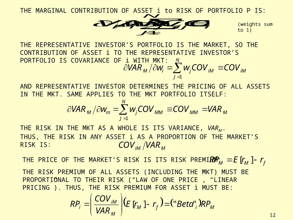
THE MARGINAL CONTRIBUTION OF ASSET i to RISK OF PORTFOLIO P IS:

THE REPRESENTATIVE INVESTOR’S PORTFOLIO IS THE MARKET, SO THE CONTRIBUTION OF ASSET i TO THE REPRESENTATIVE INVESTOR’S PORTFOLIO IS COVARIANCE OF i WITH MKT:

iM

N

JiMjiM COVCOVwwVAR

1

AND REPRESENTATIVE INVESTOR DETERMINES THE PRICING OF ALL ASSETS IN THE MKT. SAME APPLIES TO THE MKT PORTFOLIO ITSELF:

MMM

N

JMMjmM VARCOVCOVwwVAR

1

THE RISK IN THE MKT AS A WHOLE IS ITS VARIANCE, VARM .THUS, THE RISK IN ANY ASSET i AS A PROPORTION OF THE MARKET’S RISK IS:

MiM VARCOV

THE PRICE OF THE MARKET’S RISK IS ITS RISK PREMIUM: fMM rrERP ][THE RISK PREMIUM OF ALL ASSETS (INCLUDING THE MKT) MUST BE PROPORTIONAL TO THEIR RISK (“LAW OF ONE PRICE”, “LINEAR PRICING”). THUS, THE RISK PREMIUM FOR ASSET i MUST BE:

MifMM

iMi RPBetarrE

VAR

COVRP ""][

(weights sum to 1)


rf

b

E[r]

Beta of Portfolio i

Expected return of Portfolio i

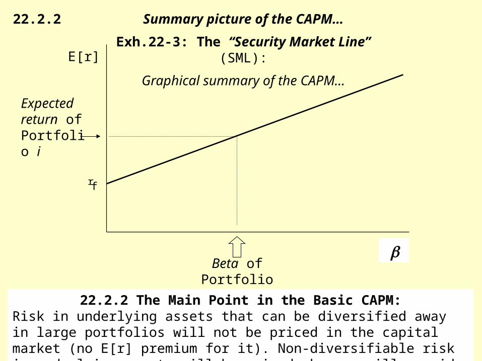
Summary picture of the CAPM…

Exh.22-3: The “Security Market Line” (SML):

Graphical summary of the CAPM…

22.2.2

22.2.2 The Main Point in the Basic CAPM:Risk in underlying assets that can be diversified away in large portfolios will not be priced in the capital market (no E[r] premium for it). Non-diversifiable risk in underlying assets will be priced, hence, will provide return premium in LR.


THE CAPM IS OBVIOUSLY A SIMPLIFICATION (of reality)… (Yes, I know that markets are not really perfectly efficient. I know we don’t all have the same expectations. I know we do not all really hold the same portfolios.) BUT IT IS A POWERFUL AND WIDELY-USED MODEL. IT CAPTURES AN IMPORTANT PART OF THE ESSENCE OF REALITY ABOUT ASSET MARKET PRICING…


22.2.4 Strengths and Weaknesses in the Basic CAPM

Strengths:• Useful as normative (what should be) prescription (it makes

sense).• As positive (what is) description the classical (original) single-

factor CAPM has some value (especially at broad-brush level, as we’ll see later).

• Provides basic and elegant intuition that may at least partly explain why more complex models work better (e.g., maybe “Fama-French factors” proxy for types of systematic risk not quantified by traditional market beta).

Weaknesses:• Without “enhancements” (e.g., Fama-French factors), the

basic single-factor CAPM is a pretty incomplete model of the expected returns of specific portfolios within an asset class.


Section 22.3

Applying the CAPM at the Asset Class Level

The basic single-factor CAPM does a pretty decent job of explaining the expected return to the real estate asset class as a whole, provided you:

• Correct the real estate returns for appraisal smoothing and lagging, and;

• Define the “market portfolio” to include all investible wealth, including real estate.

For the former purpose, you can accumulate the contemporaneous plus lagged covariances between the real estate index and the market portfolio. Or you can use “unsmoothed” or transactions-based real estate indexes.

For the latter, you can define the market portfolio as a stylized “National Wealth Portfolio” (NWP) consisting of one-third shares each of stocks, bonds, and real estate.

17

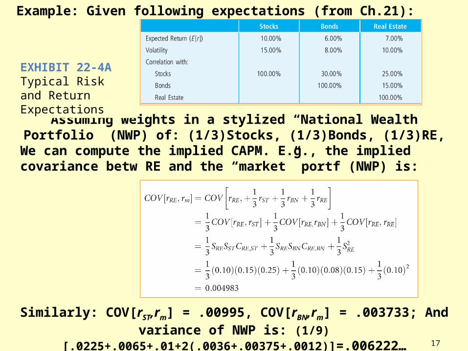
Example: Given following expectations (from Ch.21):

Assuming weights in a stylized “National Wealth Portfolio” (NWP) of: (1/3)Stocks, (1/3)Bonds, (1/3)RE,

We can compute the implied CAPM. E.g., the implied covariance betw RE and the “market” portf (NWP) is:

Similarly: COV[rST,rm] = .00995, COV[rBN,rm] = .003733; And variance of NWP is: (1/9)[.0225+.0065+.01+2(.0036+.00375+.0012)]=.006222…

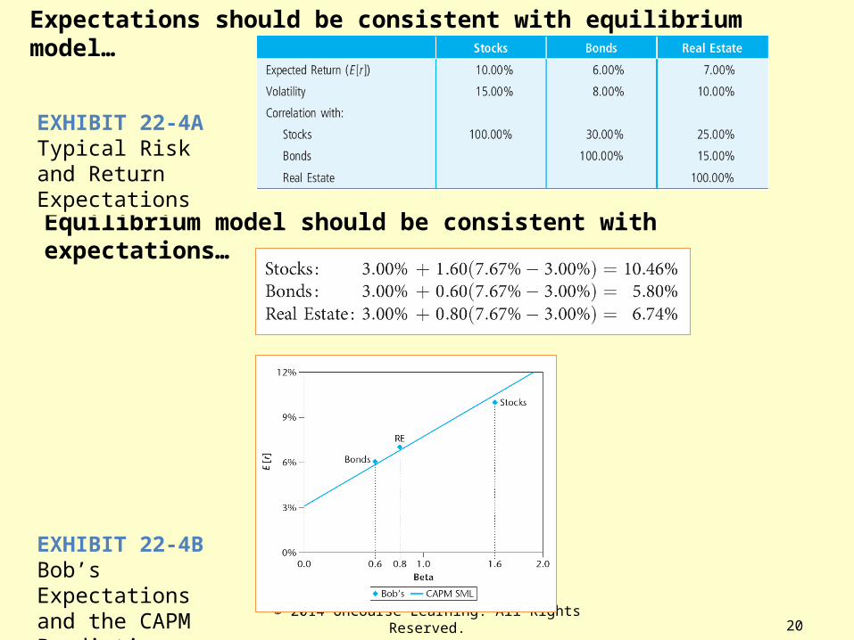
EXHIBIT 22-4ATypical Risk and ReturnExpectations


Example: Given following expectations (from Ch.21):

NWP = (1/3 each ST, BN, RE) VAR[NWP]=.006222, and: COV[rST,rm]=.004983, COV[rST,rm]=.00995, COV[rBN,rm]=.003733.

We can compute betas wrt NWP as follows:

Which, with the above betas implies CAPM expected returns as follows (assuming riskfree rate = 3%):

NWP expected return is: E[rm] = (1/3)(10%+6%+7%) = 7.67%



CAPM prediction plots on diagonal line (SML), Exh.22-4A expectations shown as diamonds.

EXHIBIT 22-4BBob’s Expectations and the CAPM Prediction


Expectations should be consistent with equilibrium model…

Equilibrium model should be consistent with expectations…


EXHIBIT 22-4BBob’s Expectations and the CAPM Prediction


22.3: Applying the Basic CAPM ACROSS asset classes

Correcting for smoothing, and defining beta wrt National Wealth…

“CAPM works.”

CAPM-predicted NCREIF E[RP] ≈ 0.75%/qtr ≈ 3%/yr.


Fama-French: CAPM by itself doesn’t work very well within the stock market:

22.4The simple 1-factor CAPM has trouble empirically within asset classes.

Enhance the basic model with additional factors that are more “tangible” than beta: (i) Stock’s Size (mkt cap), & (ii) Stock’s Book/Market Value Ratio. The market apparently associates these with “risk”.

Exh.22-5

Source: Reproduced from Fama and French (2004), Figure 3.


Size - Total Return vs Beta (NCREIF)

R&D S

R&D M

R&D L

Apt S

Apt M

Apt L

Whr S

Whr M

Whr L

CBD S

CBD M

CBD L

Sub S

Sub M

Sub L

Ret S

Ret MRet L

0.00%

2.00%

4.00%

6.00%

8.00%

10.00%

12.00%

14.00%

0.00 0.20 0.40 0.60 0.80 1.00 1.20 1.40 1.60 1.80 2.00

Beta (NCREIF)

To

tal

Ret

urn

Apts

Retail

Warehouses

R&D Space

Office

NCREIF portfolio avg returns and beta wrt NPI (1984-2003) by property size and type

The market pays more attention to tangible aspects of properties, most notably property size and quality (whether a property is “institutional” or not), and property usage type (e.g., office bldgs are “lower risk”?)

Source: Pai & Geltner, JPM (2007)


CBD-Big

CBD-Med

CBD-Sm

Sub-Big

Sub-Med

Sub-SmInd-Big

Ind-MedInd-Sm

Apt-Big

Apt-Med

Apt-Sm

Ret-Big

Ret-Med

Ret-Sm

0.5%

1.0%

1.5%

2.0%

2.5%

3.0%

0.6 0.8 1 1.2 1.4

Ex P

ost R

isk

Prem

ium

(/Q

tr, 2

000-

2011

)

Beta wrt NPI, 2000-2011

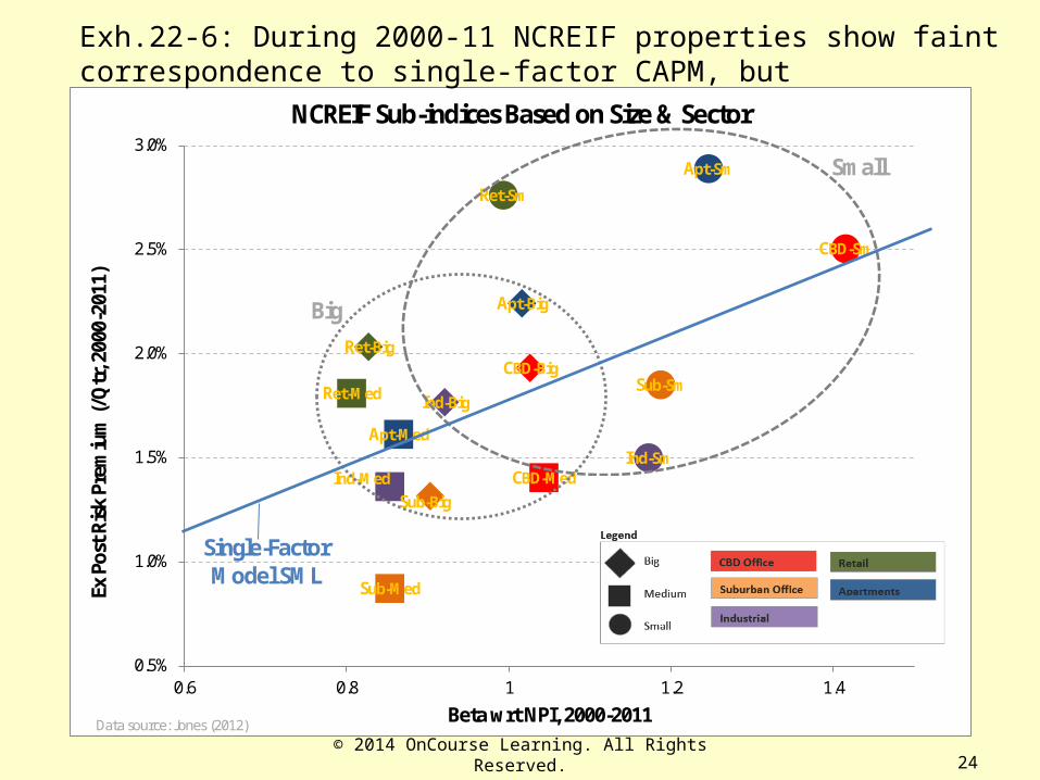
NCREIF Sub-indices Based on Size & Sector

Data source: Jones (2012)

Small

Big

Single-Factor Model SML

Exh.22-6: During 2000-11 NCREIF properties show faint correspondence to single-factor CAPM, but


11.2.6 Variation in Return Expectations Across Property Types

0%

2%

4%

6%

8%

10%

12%

14%

Mal

ls

Str

ip C

trs

Ind

ust.

Ap

ts

Sub

urb.

Off

Ch

icag

o O

ff.

Man

h O

ff

*Source: PwC Real Estate Investor Survey,2ndt quarter 2011

Malls Strip Ctrs Indust. Apts Suburb.OffChicago Off. Manh Off

Institutional 9.69% 8.97% 8.76% 8.78% 9.11% 9.55% 7.81%

Non-institutional 11.61% 11.32% 11.59% 10.98% 10.40% 12.43% 9.44%

Exh.11-8a: Investor Total Return Expectations (IRR) for Various Property Types*

Greater E[r] spread between “Instl” vs “Non-Instl” than among differ prop mkt sectors.

Recall from Ch.11…


0%

2%

4%

6%

8%

10%

12%

Mal

ls

Str

ip C

trs

Ind

ust.

Ap

ts

Sub

urb.

Off

Ch

icag

o O

ff.

Man

h O

ff

*Source: PwC Rea Estate Investor Survey, 2nd quarter 2011

Malls Strip Ctrs Indust. Apts Suburb.OffChicago

Off. Manh Off

Institutional 7.50% 7.40% 7.76% 6.29% 8.04% 8.33% 6.00%

Non-institutional 10.29% 9.90% 10.18% 7.99% 9.58% 10.50% 8.13%

Exh.11-8b: Investor Cap Rate Expectations for Various Property Types*

“Non-Instl” props have higher cap rates (income yields)…

Recall from Ch.11…


“Institutional” (aka “Investment Grade”) properties (larger, in primary mkts) exhibit different price behavior than smaller (“mom & pop”) properties, as seen in CCRSI…

Reflects different sources of financing (non-bank vs bank), different owner/investor clienteles (natl/intl instns vs local/users), different asset mkt segments.

100

110

120

130

140

150

160

170

180

190

200

210

22012

/1/1

999

6/1/

2000

12/1

/200

0

6/1/

2001

12/1

/200

1

6/1/

2002

12/1

/200

2

6/1/

2003

12/1

/200

3

6/1/

2004

12/1

/200

4

6/1/

2005

12/1

/200

5

6/1/

2006

12/1

/200

6

6/1/

2007

12/1

/200

7

6/1/

2008

12/1

/200

8

6/1/

2009

12/1

/200

9

6/1/

2010

12/1

/201

0

6/1/

2011

12/1

/201

1

1999

Val

ue =

100

CoStar CCRSI, Investment vs General Commercial Properties: Same-property (repeat-sales) Prices, 2000-2012

CCRSI General Property

CCRSI Investment Property

Data source: CoStar Group Inc. Index values as of June 2012.

2001-10: RS obs RS $volGeneral 70% 21%Investment 30% 79%All 100% 100%

“Non-Instl” props also have higher same-property price appreciation…


Simple Classical CAPM “Beta” β

Exp

ecte

d R

etu

rn E

[r]

E[r]

β

E[r]

E[r]

β

β

Bonds

Real Est

Stocks

1-Factor CAPM Across & Within Asset Classes…


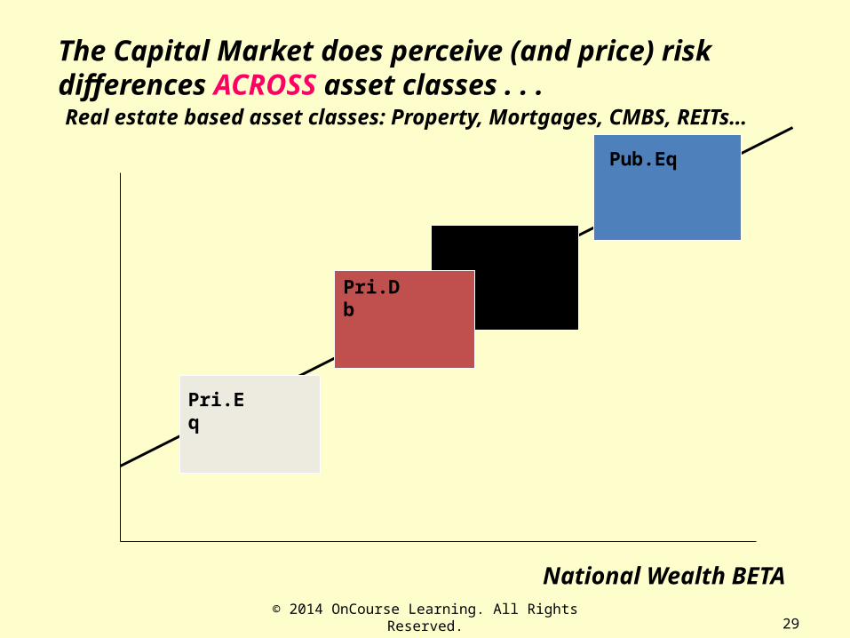
The Capital Market does perceive (and price) risk differences ACROSS asset classes . . .

National Wealth BETA

Pub.Eq

Pub.Db

Pri.Db

Pri.Eq

Real estate based asset classes: Property, Mortgages, CMBS, REITs…


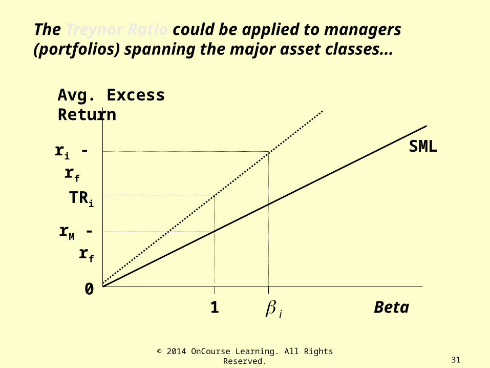
A CAPM-based method to adjust investment performance for risk: The Treynor Ratio...

Avg. Excess Return

Beta

SML

1

rM - rf

0

ri - rf

i

TRi

Based on “Risk Benchmark”

TRi = (ri - rf) / βi = slope of dashed line


The Treynor Ratio could be applied to managers (portfolios) spanning the major asset classes...

Avg. Excess Return

Beta

SML

1

rM - rf

0

ri - rf

i

TRi


The Beta can be estimated based on the “National Wealth Portfolio” ( = (1/3)Stocks + (1/3)Bonds + (1/3)RE ) as the mixed-asset “Risk Benchmark”. . .

Beta

SML

1

rM - rf

0

ri - rf

i

TRi

Based on “National Wealth Portfolio”

33

Summarizing Chapter 22: Equilibrium Asset Price Modeling & Real Estate• Like the MPT on which it is based, equilibrium asset price modeling (the CAPM

in particular) has substantial relevance and applicability to real estate when applied at the broad-brush level ( across asset classes ).

• At the fundamental property level (unlevered), real estate in general tends to be a low-beta, low-return asset class in equilibrium, but certainly not riskless, requiring (and providing) some positive risk premium (ex ante).

• CAPM type models can provide some guidance regarding the relative pricing of real estate as compared to other asset classes (“Should it currently be over-weighted or under-weighted?”), and…

• CAPM-based risk-adjusted return measures (such as the Treynor Ratio) may provide a basis for helping to judge the performance of multi-asset-class investment managers (who can allocate across asset classes).*

• Within the private real estate asset class, the CAPM is less effective at distinguishing between the relative levels of risk among real estate market segments, implying (within the state of current knowledge) a generally flat security market line across prop asset mkt segments. (not across derivatives w different leverage)

• This holds implications for tactical portfolio investment research & policy within the private real estate asset class: Search for market segments with a combination of high asset yields and high rental growth opportunities: Such apparent “bargains” present favorable risk-adjusted ex ante returns.

* Treynor Ratio requires a single-risk-factor asset pricing model.

Documents

Chapter 22 Equilibrium Asset Pricing © 2014 OnCourse Learning. All Rights Reserved.1