Chapter 15

Extended Applications

15.1. Introduction

In this chapter we will illustrate how the techniques developed in Parts II and III can be used to model systems and subsystems whose charac- teristics are significantly different from those of the centralized systems previously used as examples. Our objective is twofold: to convey the range of applicability of these techniques, and to indicate the sorts of “creative approaches” that have proven successful.

Our presentation will consist of five example application areas: com- puter communication networks (IBM’S SNA), local area networks (Ether- net>, software resources, database concurrency control, and operating sys- tem algorithms (the SRM in IBM’s MVS system). Each application is discussed in a separate section. The sections are brief; further details can be obtained from the papers cited in Section 15.8.

15.2. Computer Communication Networks

Computer communication networks use a variety of flow control policies to achieve high throughput, low delay, and stability. Here, we model the flow control policy of IBM’s System Network Architecture (SNA).

SNA routes messages from sources to destinations by way of intermedi- ate nodes which temporarily buffer the messages. Message buffers are a scarce resource. The flow control policy regulates the flow of messages between source/destination pairs in an effort to avoid problems such as deadlock and starvation, which could result from poor buffer management.

SNA has a window flow control policy. The key control parameter is the window size, W. When a source starts sending messages to a particu- lar destination, a pacing count at the source is initialized to the value of W. This pacing count is decremented every time a message is sent. If the pacing count reaches zero, the transmission of messages is halted. When the first message of a window reaches the destination, a pacing

336

15.2. Computer Communication Networks 331

response is returned to the source. Upon receipt, the source increments the current value of the pacing count by W. Another pacing response is sent to the source by the destination each time an additional W messages have been received. Thus, the maximum number of messages that can be en route from source to destination at any time is 2 W- 1.

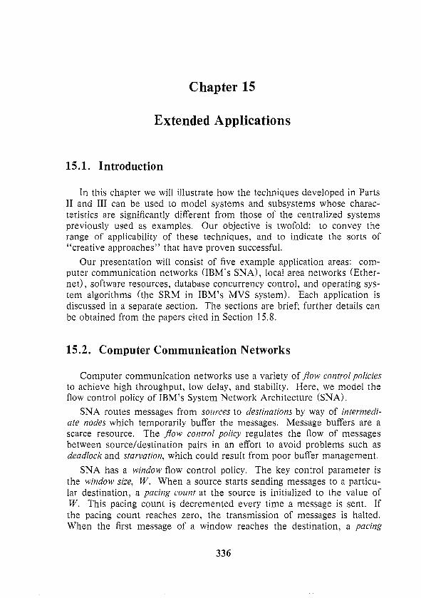
Our objective is to model the “response time” of messages between a single source/destination pair - the average time required for messages to flow from source to destination. The most convenient model, in terms of simplicity and ease of evaluation, is an open queueing network. There are M centers, representing the source node, the destination node, and M-2 intermediate nodes. (Obviously, M is determined by adding two to the number of intermediate nodes.) Customers, which represent mes- sages, arrive at the source node at rate X. They flow from node to node, requiring D units of service at each node. This model is shown in Figure 15.1.

Arrival

L%c+qJ-D-..*-D- Source Source (Service demand D at each center) (Service demand D at each center) Destination Destination

Figure 15.1 - Open Model of SNA Flow Control ( @ 1982 IEEE)

Response times can be calculated easily for this model. Unfortunately, the model makes a significant simplifying assumption which impacts the applicability of the results: there is no representation of the flow control policy! The source continues to transmit, regardless of the number of outstanding messages.

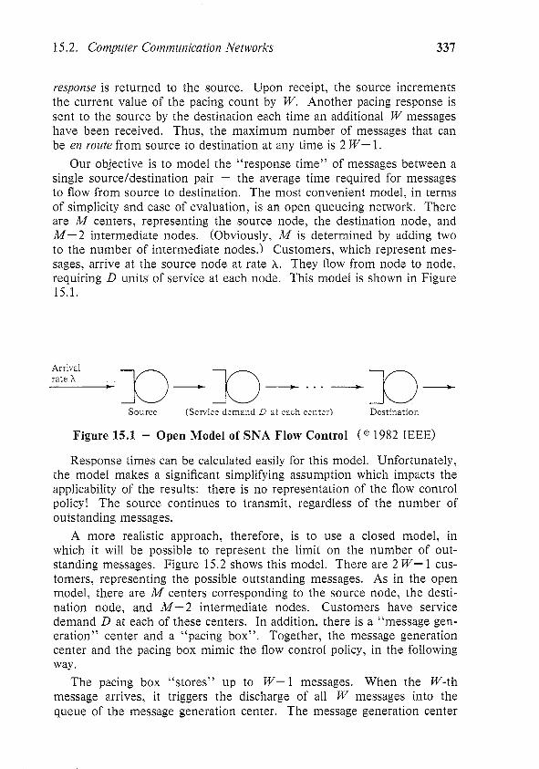
A more realistic approach, therefore, is to use a closed model, in which it will be possible to represent the limit on the number of out- standing messages, Figure 15.2 shows this model. There are 2 W- 1 cus- tomers, representing the possible outstanding messages. As in the open model, there are M centers corresponding to the source node, the desti- nation node, and M-2 intermediate nodes. Customers have service demand D at each of these centers. In addition, there is a “message gen- eration” center and a “pacing box”. Together, the message generation center and the pacing box mimic the flow control policy, in the following way.

The pacing box “stores” up to W-l messages. When the W-th message arrives, it triggers the discharge of all W messages into the queue of the message generation center. The message generation center

338 Perspective: Extended Applications

has service rate X; as long as its queue is non-empty, it will generate mes- sage traffic at this rate. A bit of thought will reveal that the arrival of the W-th message to the pacing box corresponds to the source’s receipt of a pacing response from the destination; such receipt carries with it the right to initiate W additional messages.

Source (Service demand D at each center) Destination

Message generation center

I I Pacing box

Figure 15.2 - Closed Model of SNA Flow Control (@ 1982 IEEE)

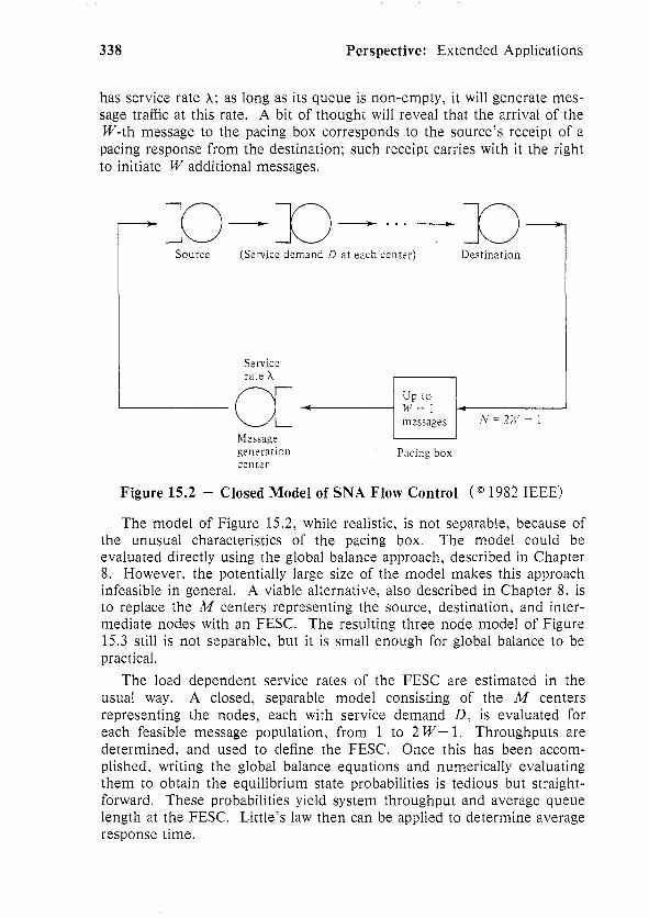
The model of Figure 15.2, while realistic, is not separable, because of the unusual characteristics of the pacing box. The model could be evaluated directly using the global balance approach, described in Chapter 8. However, the potentially large size of the model makes this approach infeasible in general. A viable alternative, also described in Chapter 8, is to replace the A4 centers representing the source, destination, and inter- mediate nodes with an FESC. The resulting three node model of Figure 15.3 still is not separable, but it is small enough for global balance to be practical.

The load dependent service rates of the FESC are estimated in the usual way. A closed, separable model consisting of the M centers representing the nodes, each with service demand D, is evaluated for each feasible message population, from 1 to 2 W- 1. Throughputs are determined, and used to define the FESC. Once this has been accom- plished, writing the global balance equations and numerically evaluating them to obtain the equilibrium state probabilities is tedious but straight- forward. These probabilities yield system throughput and average queue length at the FESC. Little’s law then can be applied to determine average response time.

15.3. Local Area Networks 339

FESC

~~.-ij--q+

Message generation Pacing box center

Figure 15.3 - FESC Representing the Message Path (@ 1982 IEEE)

One assumption made by this modelling approach is that the only traffic passing through a node is due to the source/destination pair of interest. This unrealistic assumption can be eliminated by modifying the separable model used to estimate the load dependent service rates of the FESC. As one approach, if the traffic at each node due to other source/destination pairs is known, it can be represented as an open class whose presence will impede the progress of messages associated with the source/destination pair of interest, with a resulting decrease in FESC rates.

Comparisons with detailed simulations indicate that this simple model- ling approach yields good accuracy.

15.3. Local Area Networks

Computer communication networks such as SNA are designed to per- form well over long distances at moderate bandwidths. Local area net- works, on the other hand, are optimized for use over moderate distances (say, 1 km.) at high bandwidths (10 MHz. or greater). Ethernet is perhaps the most widely known and used local area network. In this sec- tion we will describe how to incorporate a representation of Ethernet into a queueing network model of a locally distributed system.

Ethernet uses a single coaxial cable to interconnect stations (comput- ers>. A station wishing to communicate with another station broadcasts a

340 Perspective: Extended Applications

packet on this channel. (Long messages are decomposed into multiple packets prior to transmission.) The packet contains the address of the destination station, plus the desired data. All stations will “see” the packet, but only the station to which the packet is addressed will copy the packet into its local memory.

Since the channel is shared by all stations, the key to Ethernet is the way in which access to the channel is controlled. Ethernet uses carrier sense multiple access with collision detection (CSMA-CD) . Multiple access means that all stations share the same channel. Carrier sense means that no station will begin to transmit a packet if it hears data from another sta- tion on the channel. Of course, a collision still can occur, because two sta- tions can begin transmitting simultaneously (or, in fact, at times that differ by as much as the propagation delay of the channel). Collision detection means that stations “listen” while they are transmitting, stop if they detect such a collision, and retly at some point in the future. In Eth- ernet, the average amount of time that a station delays before such a retry increases with the load on the channel, with the result that stability is achieved.

The implementation of Ethernet is complex, and an attempt to incor- porate a detailed representation in a queueing network model would be ill-advised. However, Ethernet is based on a simple underlying policy. It is possible to represent the behavior of this policy in a queueing network model. Further, simulation results and measurements indicate that such a model yields accurate results. The approach that we will use is a two- level hierarchical model. At the low level we will determine the eficiency of Ethernet (the proportion of its bandwidth devoted to useful work) as a function of the instantaneous load (the number of stations simultaneously desiring to transmit packets). The results of this analysis will be used to define an FESC, which will be used to represent the channel in a system- level model.

Imagine time to be divided into slots whose duration, S, is equal to the round-trip propagation time of the channel. (This is the time required for a collision to be detected by all stations.) Consider a slot during which some number of stations n > 0 desire to transmit packets. If no station transmits, the slot is wasted. If exactly one station transmits, that station acquires the channel and continues transmitting until it has finished sending its packet. If more than one station transmits, a collision occurs and the slot is wasted. The Ethernet control policy attempts to maximize the probability that exactly one station transmits during a slot by allowing each station to transmit with probabil- ity l/n when n stations desire to use the channel. (The actual imple- mentation differs from this policy because the value of n is not known, and must be estimated by each station.)

15.3. Local Area Networks 341

If n stations desire to use the channel and each transmits indepen- dently with probability l/n, then the probability that any of the stations successfully acquires the channel during a particular slot is equal to the probability that exactly one station transmits, or:

i I

n-1 A = 1-L

n

The average number of slots devoted to contention (collisions) before a successful acquisition by some station is:

c = z i A (1-A)’ = y

i=l

For n > 0 the channel has, by definition, no idle periods; time consists of contention intervals interleaved with transmission intervals. The efficiency of the channel at instantaneous load n can be expressed as:

E(n) = length of a transmission interval length of a transmission interval -I- length of a contention interval

The length of a transmission interval equals the average packet length in bits, P, divided by the network bandwidth in bits per second, B. The length of a contention interval equals the expected number of slots devoted to contention, C, multiplied by the slot duration, S (a parameter of the configuration, related to the length of the network). In other words:

E(n) = PIB P/B + CxS

Given P, B, and S, efficiencies are calculated algebraically for each feasi- ble value of n. An FESC then is defined as follows:

p(n) = B/P x E(n)

In other words, the rate at which the Ethernet delivers packets is equal to its maximum theoretical capacity in packets per second (B/P) multiplied by the proportion of that capacity that is devoted to useful work when there are n stations desiring to transmit packets (E(n)). This FESC is used to represent the Ethernet in a system-level model.

As noted earlier, comparisons with simulation results and with meas- urements indicate that this simple modelling approach yields good accu- racy. The analysis can be extended to represent the (non-negligible) effect of packet size variability on performance. The same two-level hierarchical approach can be used to represent other local area networks. For example, a corresponding analysis has been done for the Cambridge ring.

342 Perspective: Extended Applications

15.4. Software Resources

The usual viewpoint in constructing queueing network models is that service centers correspond to hardware resources. It also is the case, though, that queueing delays in computer systems can arise from conten- tion for software resources: operating system critical sections, non- reentrant software modules, etc. In this section we consider the use of queueing network models to evaluate software system structures.

Our approach will be to define a software-level queueing network model in which customers, as usual, correspond to users, but in which service centers correspond to software modules. The service demand at each center will be equal to the time the customer spends executing the corresponding software module. The queueing delay at each center, cal- culated when the model is evaluated, will be an estimate of the time the customer is blocked awaiting access to the corresponding software module. A reentrant software module will be represented as a delay center, since a customer is never blocked awaiting access. A non- reentrant module will be represented as a queueing center, since only one customer can be executing it at a time.

Obviously, the service demand at each center in the software-level model includes various service requirements and queueing delays incurred in executing the corresponding software module on the underly- ing computer system. This service demand can be thought of as the “response time” of the user once access to the software module has been granted. This service demand will be estimated using a more conven- tional hardware-level queueing network model, in which customers correspond to users executing software modules, and centers correspond to hardware resources. The service demands are easily obtained for this hardware-level model, but the customer population is not known, because the degree of concurrency at the hardware level depends upon the extent to which users are blocked awaiting access to modules at the software level. Thus, an iterative solution is required, in which the hardware-level model provides service demand estimates for the software-level model, which in turn provides customer population estimates for the hardware- level model.

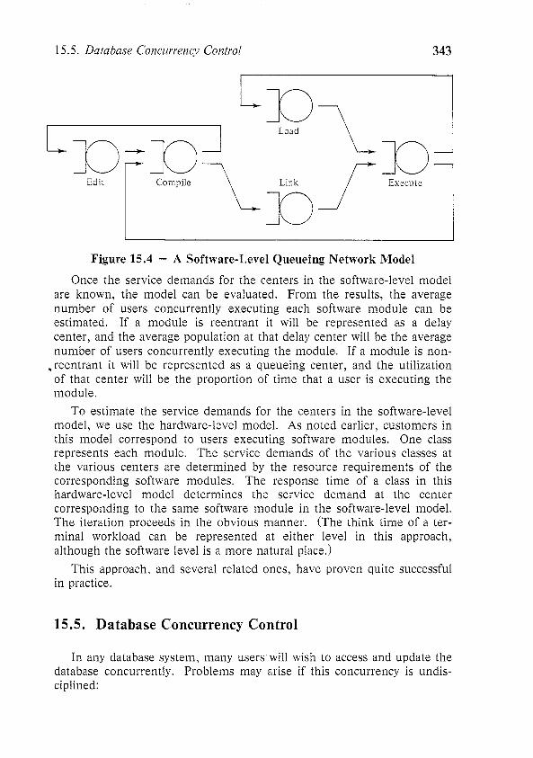
A simple example of a software-level model is shown in Figure 15.4. There are centers corresponding to various software activities: editing, compilation, linking, loading, and execution. There are various possible “execution sequences”: edit and compile; compile, link, and execute; load and execute; etc. Each execution sequence is represented as a separate customer class. The number of customers in each class is the number of users performing the corresponding execution sequence.

15.5. Database Concurrency Control 343

Figure 15.4 - A Software-Level Queueing Network Model

Once the service demands for the centers in the software-level model are known, the model can be evaluated. From the results, the average number of users concurrently executing each software module can be estimated. If a module is reentrant it will be represented as a delay center, and the average population at that delay center will be the average number of users concurrently executing the module. If a module is non-

-reentrant it will be represented as a queueing center, and the utilization of that center will be the proportion of time that a user is executing the module.

To estimate the service demands for the centers in the software-level model, we use the hardware-level model. As noted earlier, customers in this model correspond to users executing software modules. One class represents each module. The service demands of the various classes at the various centers are determined by the resource requirements of the corresponding software modules. The response time of a class in this hardware-level model determines the service demand at the center corresponding to the same software module in the software-level model. The iteration proceeds in the obvious manner. (The think time of a ter- minal workload can be represented at either level in this approach, although the software level is a more natural place.)

This approach, and several related ones, have proven quite successful in practice.

15.5. Database Concurrency Control

In any database system, many users will wish to access and update the database concurrently. Problems may arise if this concurrency is undis- ciplined:

344 Perspective: Extended Applications

0 The database may become inconsistent because of an unfortunate inter- leaving of reads and writes by various users.

0 Even if the database remains consistent, individual users may “see” inconsistent views, again because of an unfortunate interleaving of activity.

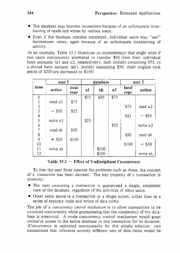
As an example, Table 15.1 illustrates an inconsistency that might arise if two users concurrently attempted to transfer $50 from their individual bank accounts (ul and u2, respectively), each initially containing $75, to a shared bank account (sh), initially containing $50: their original total assets of $200 are decreased to $150!

user 1 database user 2 time

action local ul sh u2 local action COPY COPY

0 $75 $50 $75 1 read ul $75 2 $75 read u2 3 - $50 $25 4 $25 - $50 5 write ul $25 6 $25 write u2 7 read sh $50 8 $50 read sh 9 + $50 $100 10 $100 + $50 11 write sh $100 12 $100 write sh

Table 15.1 - Effect of Undisciplined Concurrency

To free the user from concern for problems such as these, the concept of a transaction has been devised. The key property of a transaction is atomicity :

l The user executing a transaction is guaranteed a single, consistent view of the database, regardless of the activities of other users.

* Orher users perceive a transaction as a single action, rather than as a series of separate reads and writes of data items.

The job of a concurrency control mechanism is to allow transactions to be executed concurrently while guaranteeing that the consistency of the data- base is preserved. A crude concurrency control mechanism would grant exclusive access to the entire database to one transaction for its duration. (Concurrency is restricted unnecessarily by this simple solution: two transactions that reference entirely different sets of data items would be

15.5. Database Concurrency Control 345

unable to proceed concurrently.) A more reasonable mechanism would grant exclusive access to various data items to one transaction for its duration. Other possibilities exist. Clearly, the presence of a concurrency control mechanism can have a significant effect on system performance - an effect somewhat analogous to that of a memory constraint. Equally clearly, a queueing network model that represents the concurrency con- trol mechanism directly will be non-separable: customers may be blocked when data items they require are held by other customers. Techniques comparable to those developed in Part III and in the other sections of this chapter are required.

In this section we consider the evaluation of a database system employing a particular, simple concurrency control mechanism. The pro- cessing of a transaction under this concurrency control mechanism is described in Table 15.2. Consider the banking example in Table 15.1. Under the concurrency control mechanism, the activities of user 1 and user 2 would constitute separate transactions. User 1 would obtain locks on data items ul and sh, and would proceed without concern for interfer- ence from others. User 2 would be granted a lock on u2 but denied a lock on sh, and would abort, releasing the lock on u2. Subsequently, user 2’s transaction would be re-submitted. (We assume that aborted transactions are re-submitted after some delay.) User 1 would be finished, so the lock on sh would be granted to user 2, who would find the value of sh equal to $100.

The effect of the concurrency control mechanism on performance is evident from this example and from Table 15.2. Some transactions abort because they are unable to obtain a lock on a required data item. From the point of view of the system, a transaction that aborts consumes resources (although not to the extent of a successful transaction). From the point of view of a user, several attempts may be required to complete a transaction successfully.

Estimating the proportion of transactions that abort and the service demands of these transactions are the keys to modelling the system. Ini- tially, though, let us assume that conflicts never occur, so all transactions complete successfully. In this case, a traditional separable queueing net- work model is suitable. Users at terminals submit transactions. The ser- vice demands of transactions can be calculated by considering their com- plexity: number of items read, number of items written, processing requirements, overhead of lock manipulation required for concurrency control, etc. Evaluating this model yields the average transaction response time and other performance measures of interest.

How can this model be extended to represent the effect of conflicts between transactions? As noted, we must estimate the proportion of transactions that abort, PLabortl, and the service demands of these

346 Perspective: Extended Applications

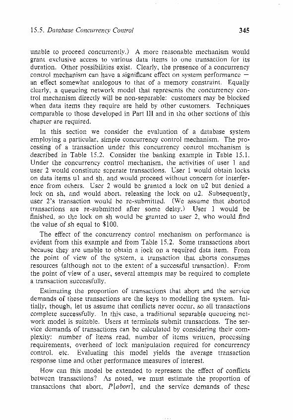
locking phase

- Request a read lock on each data item whose value is required. A read lock will be granted if no other transaction currently holds a write lock on the item.

- Request a write lock on each data item that is to be written. A write lock will be granted if no other transaction currently holds either a read lock or a write lock on the item.

- If any lock is refused, abort, releasing all locks previously granted to the transaction.

processing phase

- Read the values of the required data items. - Based on these values, compute the values of the data items

to be written. - Update the values of the data items to be written. termination phase

- Release all read and write locks held by the transaction.

Table 15.2 - Steps in Processing a Transaction

transactions. Given this information, we could adjust the service demands of transactions in the model to be:

(1 - PLabortl) X (service demands of a successful transaction) +

PIabort X (service demands of an aborted transaction)

The model could be evaluated using this parameterization to yield response times for each submission of a transaction. To compute the effective response time to successfully complete a transaction we would multiply the response time of each submission by the average number of submissions required. (Obviously, a homogeneity assumption is employed here.) The average number of submissions required is:

1 X (1 - PIabort]) -I-

2 X (1 - Piabort]) X P[abort] -I-

3 X (1 - Plabortl) X P[abort]’ +

1 = 1 - P[abort]

15.6. Operating System Algorithms 341

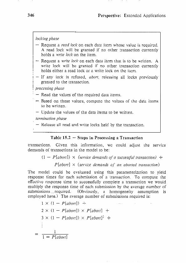
The proportion of transactions that abort depends on many factors, including the average number of active transactions (if few transactions are active simultaneously, then the probability of conflict is low) and the average number of data items read and written by each transaction, rela- tive to the total number of items in the database (if each transaction locks a very small proportion of the items in the database, then the probability of conflict is low). As an example, one particularly simple approach is to assume that each transaction requires read locks on r of the I items in the database, chosen at random, and write locks on w of these I items, also chosen independently and at random. A probabilistic analysis then yields PIabort]. This analysis is based on reasoning such as the follow- ing: If N transactions are active, they hold N X PV write locks. An arriving transaction will be able to acquire all of its r required read locks with probability:

(More accurate estimates of P[abortl can be obtained from more detailed submodels, evaluated either probabilistically or using simulation.)

The service demands of an aborted transaction can be estimated roughly as one half of the lock manipulation overhead of a successful transaction. (We expect half the required locks to be obtained before one is denied; these must be released when the transaction aborts.) In addi- tion, by assumption aborted transactions are re-submitted after some delay. This can be represented by adding a delay center to the model, or by adjusting the “think time” downwards in a manner analogous to that used for service demands.

The average number of active transactions, which is a key parameter required to estimate P[abortl, is an output of the model. This suggests the iterative evaluation scheme outlined in Algorithm 15.1. We have left many details unspecified, and have made a number of simplifying assumptions concerning the nature of the system and of the concurrency control mechanism. The basic iterative approach of Algorithm 15.1 is relatively general, however.

15.6. Operating System Algorithms

During the design of an operating system, extremely subtle perfor- mance questions may arise that require certain subsystems to be modelled at a level of detail greater than we have considered thus far. Examples of such questions include the design of complex resource allocation

348 Perspective: Extended Applications

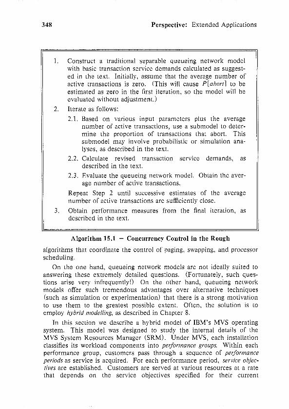
1. Construct a traditional separable queueing network model with basic transaction service demands calculated as suggest- ed in the text. Initially, assume that the average number of active transactions is zero. (This will cause PLabortl to be estimated as zero in the first iteration, so the model will be evaluated without adjustment.)

2. Iterate as follows: 2.1, Based on various input parameters plus the average

number of active transactions, use a submodel to deter- mine the proportion of transactions that abort. This submodel may involve probabilistic or simulation ana- lyses, as described in the text.

2.2. Calculate revised transaction service demands, as described in the text.

2.3. Evaluate the queueing network model. Obtain the aver- age number of active transactions.

Repeat Step 2 until successive estimates of the average number of active transactions are sufficiently close.

3. Obtain performance measures from the final iteration, as described in the text.

Algorithm 15.1 - Concurrency Control in the Rough

algorithms that coordinate the control of paging, swapping, and processor scheduling.

On the one hand, queueing network models are not ideally suited to answering these extremely detailed questions. (Fortunately, such ques- tions arise very infrequently!) On the other hand, queueing network models offer such tremendous advantages over alternative techniques (such as simulation or experimentation) that there is a strong motivation to use them to the greatest possible extent. Often, the solution is to employ hybrid modeling, as described in Chapter 8.

In this section we describe a hybrid model of IBM’s MVS operating system. This model was designed to study the internal details of the MVS System Resources Manager (SRM). Under MVS, each installation classifies its workload components into performance groups. Within each performance group, customers pass through a sequence of performance periods as service is acquired. For each performance period, service objec- tives are established. Customers are served at various resources at a rate that depends on the service objectives specified for their current

15.7. Summary 349

performance period. (For example, a customer’s susceptibility to swap- ping will depend on that customer’s current performance period.) In addition, goals are established for the utilizations of various resources. These goals impose additional constraints on scheduling decisions. It is the job of the SRM to reconcile these many objectives by making appropriate long-term and short-term resource allocation decisions.

Figure 15.5 illustrates the structure of the two-level hierarchical hybrid model that allowed the internal algorithms of the SRM to be represented. There are two workload components: TSO (timesharing) and batch. In the high-level model, customer arrivals and the operation of the SRM are represented. Two principal SRM modules are represented explicitly. Swap Analysis keeps track of the attained service of each customer and determines if a swap is to be performed. Resource Monitor calculates tar- get multiprogramming levels, invokes Swap Analysis if necessary, and collects various statistics. These statistics are used in an overhead sub- model to determine the overhead service demands of the operating sys- tem. The high-level model is evaluated using simulation.

In the low-level model, the central subsystem is represented. Paging activity is determined by a submodel that has knowledge of the particular paging policy of interest. The low-level model is evaluated using tech- niques from Parts II and III.

The hybrid solution of this model proceeds iteratively. The high-level model determines the multiprogramming mix and the overhead service demands, and supplies these to the low-level model. The low-level model determines throughputs and utilizations, which allow the high- level model to calculate the time of the next completion and to make resource allocation decisions.

Of course, representing the internal algorithms of the SRM is a level of detail far beyond that which is appropriate for capacity planning and performance projection applications. Still, this hybrid model was success- ful at answering detailed questions concerning SRM behavior. Evaluation of the model was estimated to be 30 to 100 times faster than would have been possible using a pure simulation approach. The modelling approach led to greater flexibility than would have been possible in direct experi- mentation on an MVS system.

15.7. Summary

This chapter has used five examples to illustrate that the applicability of queueing network models extends well beyond the confines of central- ized systems with simple characteristics. We have studied models of computer communication networks, local area networks, software

Perspective: Extended Applications

SIMULATION

BATCH WORKLOAD

Arrival - JOB

Departure ENTRY SUBSYSTEM

A

T

SYSTEhl RESOURCES MANAGER

TSO WORKLOAD

t RESOURCE SWAP MONITOR ANALYSIS

r

r

STATISTICAL MODEL FOR OVERHEAD

I

Y

ANALYSIS

L

Figure 15.5 - A Detailed Hybrid Model of the MVS SRM

15.8. References 351

resources, database concurrency control, and operating system.algorithms. These models have employed techniques such as FESCs with global bal- ance, FESCs whose service rates are determined through probabilistic analysis, two-level hierarchical iteration, and hybrid modelling. These techniques, combined with good knowledge of the system being modelled and a modicum of inventiveness, can solve a wide variety of computer system analysis problems.

15.8. References

Queueing theory has been used widely in the detailed analysis of com- puter communication network protocols. The use of queueing network models to evaluate networks and to represent them in system-level models is more recent. A useful genera1 discussion of this area is the book by Schwartz 119771. The SNA flow control model in Section 15.2 was constructed by Schwartz 119821; this paper is the source of Figures 15.1, 15.2, and 15.3.

Local area networks have received widespread attention recently. Eth- ernet was described originally by Metcalfe and Boggs [19761. The Ether- net mode1 in Section 15.3 was developed by Almes and Lazowska [19791. King and Mitrani [19821 discuss a similar model of the Cambridge ring.

The technique for modelling software resources described in Section 15.4 is similar to one described by Agre and Tripathi [19821. Other approaches are described by Smith and Browne [19801, Agrawal and Buzen [19831, and Jacobson and Lazowska [19831.

The modelling of database concurrency control mechanisms is the sub- ject of much recent research activity. Sevcik [19831 provides a survey of various approaches. An excellent discussion of the issues involved, including a framework for classifying mechanisms, is provided by Bern- stein and Goodman [19811.

An overview of an early version of the MVS SRM is given by Lynch and Page [19741. The hybrid hierarchical mode1 in Section 15.6 was developed by Chiu and Chow 119781; their paper is the source of Figure 15.5. Buzen [1978] describes a queueing network model of MVS that is better suited to capacity planning applications.

[Agrawal & Buzen 19831 Subhash C. Agrawal and Jeffrey P. Buzen. The Aggregate Server Method for Analyzing Serialization Delays in Computer Systems. Transactions on Computer Systems 1,2 (March 19831, 116-143.

352 Perspective: Extended Applications

[Agre & Tripathi 19821 Jon R. Agre and Satish K. Tripathi. Modelling Reentrant and Non- Reentrant Software. Proc. ACM SIGMETRICS Conference on Meas- urement and Modeling of Computer Systems (19821, 163-178.

[Almes & Lazowska 19791 Guy T. Almes and Edward D. Lazowska. The Behavior of Ethernet- Like Computer Communication Networks. Proc. 7th Symposium on Operating Systems Principles (19791, 66-81. Copyright @ 1979 by the Association for Computing Machinery.

[Bernstein & Goodman 19811 Philip A. Bernstein and N. Goodman. Concurrency Control in Distri- buted Database Systems. Computing Surveys 13,2 (June 19811, 185- 221.

[Buzen 19781 Jeffrey P. Buzen. A Queueing Network Model of MVS. Computing Surveys 10,3 (September 19781, 319-331.

[Chiu and Chow 19781 Willy W. Chiu and We-Min Chow. A Performance Model of MVS. IBMSystems Journal 17,4 (19781, 444-462.

[Jacobson & Lazowska 19831 Patricia A. Jacobson and Edward D. Lazowska. A Reduction Tech- nique for Evaluating Queueing Networks with Serialization Delays. Proc. IFIP W.G. 7.3 International Symposium on Computer Performance Modeling, Measurement, and Evaluation (1983), 45-59.

[King & Mitrani 19821 Peter J.B. King and Israel Mitrani. Modelling the Cambridge Ring. Proc. ACM SIGMETRICS Conference on Measurement and Modeling of Computer Systems (19821, 250-258.

[Lynch & Page 19741 H.W. Lynch and J.B. Page. The OS/V’S2 Release 2 System Resources Manager. IBM Systems Journal 13,4 (19741, 274-291.

[Metcalfe & Boggs 19761 Robert M. Metcalfe and David R. Boggs. Ethernet: Distributed Packet Switching for Local Computer Networks. CACM 19,7 (July 1976), 395-404.

[Schwartz 19771 Mischa Schwartz. Computer Communication Network Design and Analysis. Prentice-Hall, 1977.

15.8. References 353

[Schwartz 19821 Mischa Schwartz. Performance Analysis of the SNA Virtual Route Pacing Control. IEEE Transactions on Communications COM-30,l (January 19821, 172-184. Copyright @ 1982 IEEE.

[Sevcik 19831 Kenneth C. Sevcik. Comparison of Concurrency Control Algorithms Using Analytic Models. Proc. IFIP Congress ‘83 (1983).

[Smith and Browne 19801 Connie Smith and J.C. Browne. Aspects of Software Design Analysis: Concurrency and Blocking. Proc. IFIP W. G. 7.3 International Sympo- sium on Computer Performance Modeling, Measurement, and Evaluation (19801, 245-253.