Embed Size (px)
Citation preview

543
Chapter 10
Spectroscopic MethodsChapter OverviewSection 10A Overview of SpectroscopySection 10B Spectroscopy Based on AbsorptionSection 10C UV/Vis and IR SpectroscopySection 10D Atomic Absorption SpectroscopySection 10E Emission SpectroscopySection 10F Photoluminescent SpectroscopySection 10G Atomic Emission SpectroscopySection 10H Spectroscopy Based on ScatteringSection 10I Key TermsSection 10J Chapter SummarySection 10K ProblemsSection 10L Solutions to Practice Exercises
An early example of a colorimetric analysis is Nessler’s method for ammonia, which was introduced in 1856. Nessler found that adding an alkaline solution of HgI2 and KI to a dilute solution of ammonia produces a yellow to reddish brown colloid, with the colloid’s color depending on the concentration of ammonia. By visually comparing the color of a sample to the colors of a series of standards, Nessler was able to determine the concentration of ammonia.
Colorimetry, in which a sample absorbs visible light, is one example of a spectroscopic method of analysis. At the end of the nineteenth century, spectroscopy was limited to the absorption, emission, and scattering of visible, ultraviolet, and infrared electromagnetic radiation. Since its introduction, spectroscopy has expanded to include other forms of electromagnetic radiation—such as X-rays, microwaves, and radio waves—and other energetic particles—such as electrons and ions.
Source URL: http://www.asdlib.org/onlineArticles/ecourseware/Analytical%20Chemistry%202.0/Text_Files.html Saylor URL: http://www.saylor.org/courses/chem108 Attributed to [David Harvey]
Saylor.org Page 1 of 124

544 Analytical Chemistry 2.0
10A Overview of Spectroscopy
The focus of this chapter is on the interaction of ultraviolet, visible, and infrared radiation with matter. Because these techniques use optical materi-als to disperse and focus the radiation, they often are identified as optical spectroscopies. For convenience we will use the simpler term spectroscopy in place of optical spectroscopy; however, you should understand that we are considering only a limited part of a much broader area of analytical techniques.
Despite the difference in instrumentation, all spectroscopic techniques share several common features. Before we consider individual examples in greater detail, let’s take a moment to consider some of these similarities. As you work through the chapter, this overview will help you focus on similarities between different spectroscopic methods of analysis. You will find it easier to understand a new analytical method when you can see its relationship to other similar methods.
10A.1 What is Electromagnetic Radiation
Electromagnetic radiation—light—is a form of energy whose behavior is described by the properties of both waves and particles. Some properties of electromagnetic radiation, such as its refraction when it passes from one medium to another (Figure 10.1), are explained best by describing light as a wave. Other properties, such as absorption and emission, are better de-scribed by treating light as a particle. The exact nature of electromagnetic radiation remains unclear, as it has since the development of quantum mechanics in the first quarter of the 20th century.1 Nevertheless, the dual models of wave and particle behavior provide a useful description for elec-tromagnetic radiation.
WAVE PROPERTIES OF ELECTROMAGNETIC RADIATION
Electromagnetic radiation consists of oscillating electric and magnetic fields that propagate through space along a linear path and with a constant ve-locity. In a vacuum electromagnetic radiation travels at the speed of light, c, which is 2.997 92 × 108 m/s. When electromagnetic radiation moves through a medium other than a vacuum its velocity, v, is less than the speed of light in a vacuum. The difference between v and c is sufficiently small (<0.1%) that the speed of light to three significant figures, 3.00 × 10⁸ m/s, is accurate enough for most purposes.
The oscillations in the electric and magnetic fields are perpendicular to each other, and to the direction of the wave’s propagation. Figure 10.2 shows an example of plane-polarized electromagnetic radiation, consisting of a single oscillating electric field and a single oscillating magnetic field.
An electromagnetic wave is characterized by several fundamental prop-erties, including its velocity, amplitude, frequency, phase angle, polariza-1 Home, D.; Gribbin, J. New Scientist 1991, 2 Nov. 30–33.
Figure 10.1 The Golden Gate bridge as seen through rain drops. Refraction of light by the rain drops produces the distorted images. Source: Mila Zinkova (commons.wikipedia.org).
Source URL: http://www.asdlib.org/onlineArticles/ecourseware/Analytical%20Chemistry%202.0/Text_Files.html Saylor URL: http://www.saylor.org/courses/chem108 Attributed to [David Harvey]
Saylor.org Page 2 of 124

545Chapter 10 Spectroscopic Methods
tion, and direction of propagation.2 For example, the amplitude of the oscillating electric field at any point along the propagating wave is
A A tt e= +sin( )2πν Φ
where At is the magnitude of the electric field at time t, Ae is the electric field’s maximum amplitude, ν is the wave’s frequency—the number of oscillations in the electric field per unit time—and Φ is a phase angle, which accounts for the fact that At need not have a value of zero at t = 0. The identical equation for the magnetic field is
A A tt m= +sin( )2πν Φ
where Am is the magnetic field’s maximum amplitude.Other properties also are useful for characterizing the wave behavior of
electromagnetic radiation. The wavelength, λ, is defined as the distance between successive maxima (see Figure 10.2). For ultraviolet and visible electromagnetic radiation the wavelength is usually expressed in nanome-ters (1 nm = 10–9 m), and for infrared radiation it is given in microns (1 μm = 10–6 m). The relationship between wavelength and frequency is
λν
=c
Another unit useful unit is the wavenumber, ν , which is the reciprocal of wavelength
νλ
=1
Wavenumbers are frequently used to characterize infrared radiation, with the units given in cm–1.2 Ball, D. W. Spectroscopy 1994, 9(5), 24–25.
Figure 10.2 Plane-polarized electromagnetic radiation showing the oscillating electric field in red and the oscil-lating magnetic field in blue. The radiation’s amplitude, A, and its wavelength, λ, are shown. Normally, elec-tromagnetic radiation is unpolarized, with oscillating electric and magnetic fields present in all possible planes perpendicular to the direction of propagation.
When electromagnetic radiation moves between different media—for example, when it moves from air into water—its frequency, ν, remains constant. Because its velocity depends upon the medium in which it is traveling, the electromagnetic radiation’s wavelength, λ, changes. If we replace the speed of light in a vacuum, c, with its speed in the medium, v, then the wavelength is
λν
=v
This change in wavelength as light passes between two media explains the refrac-tion of electromagnetic radiation shown in Figure 10.1.
directionof
propagation
elec
tric
fiel
d
mag
netic field
λ
A
Source URL: http://www.asdlib.org/onlineArticles/ecourseware/Analytical%20Chemistry%202.0/Text_Files.html Saylor URL: http://www.saylor.org/courses/chem108 Attributed to [David Harvey]
Saylor.org Page 3 of 124

546 Analytical Chemistry 2.0
Example 10.1
In 1817, Josef Fraunhofer studied the spectrum of solar radiation, observ-ing a continuous spectrum with numerous dark lines. Fraunhofer labeled the most prominent of the dark lines with letters. In 1859, Gustav Kirch-hoff showed that the D line in the sun’s spectrum was due to the absorption of solar radiation by sodium atoms. The wavelength of the sodium D line is 589 nm. What are the frequency and the wavenumber for this line?
SOLUTION
The frequency and wavenumber of the sodium D line are
νλ
= =××
= ×−
−c 3 00 1010
5 09 108
914 1.
.m/s
589 ms
νλ
= =×
× = ×−
−1 1589 10
11 70 10
94 1
mm
100 cmcm.
Practice Exercise 10.1Another historically important series of spectral lines is the Balmer series of emission lines form hydrogen. One of the lines has a wavelength of 656.3 nm. What are the frequency and the wavenumber for this line?
Click here to review your answer to this exercise.
PARTICLE PROPERTIES OF ELECTROMAGNETIC RADIATION
When matter absorbs electromagnetic radiation it undergoes a change in energy. The interaction between matter and electromagnetic radiation is easiest to understand if we assume that radiation consists of a beam of en-ergetic particles called photons. When a photon is absorbed by a sample it is “destroyed,” and its energy acquired by the sample.3 The energy of a photon, in joules, is related to its frequency, wavelength, and wavenumber by the following equalities
E hhc
hc= = =νλ
ν
where h is Planck’s constant, which has a value of 6.626 × 10⁻³⁴ J . s.
Example 10.2
What is the energy of a photon from the sodium D line at 589 nm?
SOLUTION
The photon’s energy is
3 Ball, D. W. Spectroscopy 1994, 9(6) 20–21.
Source URL: http://www.asdlib.org/onlineArticles/ecourseware/Analytical%20Chemistry%202.0/Text_Files.html Saylor URL: http://www.saylor.org/courses/chem108 Attributed to [David Harvey]
Saylor.org Page 4 of 124

547Chapter 10 Spectroscopic Methods
Ehc
= =× ⋅ ×
×
−
λ( .6 626 10 10
589 10
34 8J s)(3.00 m/s)−−
−= ×9
193 37 10m
J.
Figure 10.3 The electromagnetic spectrum showing the boundaries between different regions and the type of atomic or molecular transition responsible for the change in energy. The colored inset shows the visible spectrum. Source: modified from Zedh (www.commons.wikipedia.org).
Practice Exercise 10.2What is the energy of a photon for the Balmer line at a wavelength of 656.3 nm?
Click here to review your answer to this exercise.
THE ELECTROMAGNETIC SPECTRUM
The frequency and wavelength of electromagnetic radiation vary over many orders of magnitude. For convenience, we divide electromagnetic radiation into different regions—the electromagnetic spectrum—based on the type of atomic or molecular transition that gives rise to the absorption or emission of photons (Figure 10.3). The boundaries between the regions of the electromagnetic spectrum are not rigid, and overlap between spectral regions is possible.
10A.2 Photons as a Signal Source
In the previous section we defined several characteristic properties of elec-tromagnetic radiation, including its energy, velocity, amplitude, frequency, phase angle, polarization, and direction of propagation. A spectroscopic measurement is possible only if the photon’s interaction with the sample leads to a change in one or more of these characteristic properties.
Types of Atomic & Molecular Transitionsγ-rays: nuclearX-rays: core-level electronsUltraviolet (UV): valence electronsVisible (Vis): valence electronsInfrared (IR): molecular vibrationsMicrowave: molecular roations; electron spinRadio waves: nuclear spin
γ-rays X-rays UV IR Microwave FM AM Long radio waves
Radio waves
Increasing Frequency (ν)
Increasing Wavelength (λ)
Visible Spectrum
Increasing Wavelength (λ) in nm
1024 1022 1020 1018 1016 1014 1012 1010 108 106 104 102 100
10-16 10-14 10-12 10-10 10-8 10-6 10-4 10-2 100 102 104 106 108
ν (s-1)
λ (nm)
400 500400 600 700
Source URL: http://www.asdlib.org/onlineArticles/ecourseware/Analytical%20Chemistry%202.0/Text_Files.html Saylor URL: http://www.saylor.org/courses/chem108 Attributed to [David Harvey]
Saylor.org Page 5 of 124

548 Analytical Chemistry 2.0
We can divide spectroscopy into two broad classes of techniques. In one class of techniques there is a transfer of energy between the photon and the sample. Table 10.1 provides a list of several representative examples.
In absorption spectroscopy a photon is absorbed by an atom or mol-ecule, which undergoes a transition from a lower-energy state to a higher-energy, or excited state (Figure 10.4). The type of transition depends on the photon’s energy. The electromagnetic spectrum in Figure 10.3, for example, shows that absorbing a photon of visible light promotes one of the atom’s or molecule’s valence electrons to a higher-energy level. When an molecule absorbs infrared radiation, on the other hand, one of its chemical bonds experiences a change in vibrational energy.
Table 10.1 Examples of Spectroscopic Techniques Involving an Exchange of Energy Between a Photon and the Sample
Type of Energy TransferRegion of
Electromagnetic Spectrum Spectroscopic Techniquea
absorption γ-ray Mossbauer spectroscopyX-ray X-ray absorption spectroscopyUV/Vis UV/Vis spectroscopy
atomic absorption spectroscopyIR infrared spectroscopy
raman spectroscopyMicrowave microwave spectroscopyRadio wave electron spin resonance spectroscopy
nuclear magnetic resonance spectroscopyemission (thermal excitation) UV/Vis atomic emission spectroscopyphotoluminescence X-ray X-ray fluorescence
UV/Vis fluorescence spectroscopyphosphorescence spectroscopyatomic fluorescence spectroscopy
chemiluminescence UV/Vis chemiluminescence spectroscopya Techniques discussed in this text are shown in italics.
Figure 10.4 Simplified energy diagram showing the absorption and emission of a photon by an atom or a molecule. When a photon of energy hν strikes the atom or molecule, absorption may occur if the differ-ence in energy, ΔE, between the ground state and the excited state is equal to the photon’s energy. An atom or molecule in an excited state may emit a photon and return to the ground state. The photon’s energy, hν, equals the difference in energy, ΔE, between the two states. ground state
exicted states
Ener
gy
hν ΔE = hν ΔE = hνhν
absorption emission
Source URL: http://www.asdlib.org/onlineArticles/ecourseware/Analytical%20Chemistry%202.0/Text_Files.html Saylor URL: http://www.saylor.org/courses/chem108 Attributed to [David Harvey]
Saylor.org Page 6 of 124

549Chapter 10 Spectroscopic Methods
When it absorbs electromagnetic radiation the number of photons pass-ing through a sample decreases. The measurement of this decrease in pho-tons, which we call absorbance, is a useful analytical signal. Note that the each of the energy levels in Figure 10.4 has a well-defined value because they are quantized. Absorption occurs only when the photon’s energy, hν, matches the difference in energy, ΔE, between two energy levels. A plot of absorbance as a function of the photon’s energy is called an absorbance spectrum. Figure 10.5, for example, shows the absorbance spectrum of cranberry juice.
When an atom or molecule in an excited state returns to a lower energy state, the excess energy often is released as a photon, a process we call emis-sion (Figure 10.4). There are several ways in which an atom or molecule may end up in an excited state, including thermal energy, absorption of a photon, or by a chemical reaction. Emission following the absorption of a photon is also called photoluminescence, and that following a chemi-cal reaction is called chemiluminescence. A typical emission spectrum is shown in Figure 10.6.
Figure 10.5 Visible absorbance spectrum for cranberry juice. The anthocyanin dyes in cranberry juice absorb visible light with blue, green, and yellow wavelengths (see Figure 10.3). As a result, the juice appears red.
Molecules also can release energy in the form of heat. We will return to this point later in the chapter.
Figure 10.6 Photoluminescence spectrum of the dye coumarin 343, which is incorporated in a reverse micelle suspended in cy-clohexanol. The dye’s absorbance spectrum (not shown) has a broad peak around 400 nm. The sharp peak at 409 nm is from the laser source used to excite coumarin 343. The broad band centered at approximately 500 nm is the dye’s emission band. Because the dye absorbs blue light, a solution of coumarin 343 appears yellow in the absence of photoluminescence. Its photo-luminescent emission is blue-green. Source: data from Bridget Gourley, Department of Chemistry & Biochemistry, DePauw University).
400 450 500 550 600 650 700 750
0.0
0.2
0.4
0.6
0.8
wavelength (nm)
abso
rban
ce
400 450 500 550 600 650wavelength (nm)
emis
sion
inte
nsity
(arb
itrar
y un
its)
Source URL: http://www.asdlib.org/onlineArticles/ecourseware/Analytical%20Chemistry%202.0/Text_Files.html Saylor URL: http://www.saylor.org/courses/chem108 Attributed to [David Harvey]
Saylor.org Page 7 of 124

550 Analytical Chemistry 2.0
In the second broad class of spectroscopic techniques, the electromag-netic radiation undergoes a change in amplitude, phase angle, polarization, or direction of propagation as a result of its refraction, reflection, scatter-ing, diffraction, or dispersion by the sample. Several representative spectro-scopic techniques are listed in Table 10.2.
10A.3 Basic Components of Spectroscopic Instruments
The spectroscopic techniques in Table 10.1 and Table 10.2 use instruments that share several common basic components, including a source of energy, a means for isolating a narrow range of wavelengths, a detector for measur-ing the signal, and a signal processor that displays the signal in a form con-venient for the analyst. In this section we introduce these basic components. Specific instrument designs are considered in later sections.
SOURCES OF ENERGY
All forms of spectroscopy require a source of energy. In absorption and scattering spectroscopy this energy is supplied by photons. Emission and photoluminescence spectroscopy use thermal, radiant (photon), or chemi-cal energy to promote the analyte to a suitable excited state.Sources of Electromagnetic Radiation. A source of electromagnetic radia-tion must provide an output that is both intense and stable. Sources of electromagnetic radiation are classified as either continuum or line sources. A continuum source emits radiation over a broad range of wavelengths, with a relatively smooth variation in intensity (Figure 10.7). A line source, on the other hand, emits radiation at selected wavelengths (Figure 10.8). Table 10.3 provides a list of the most common sources of electromagnetic radiation.Sources of Thermal Energy. The most common sources of thermal energy are flames and plasmas. Flames sources use the combustion of a fuel and an oxidant to achieve temperatures of 2000–3400 K. Plasmas, which are hot, ionized gases, provide temperatures of 6000–10 000 K.
Table 10.2 Examples of Spectroscopic Techniques That Do Not Involve an Exchange of Energy Between a Photon and the Sample
Region of Electromagnetic Spectrum Type of Interaction Spectroscopic Techniquea
X-ray diffraction X-ray diffractionUV/Vis refraction refractometry
scattering nephelometryturbidimetry
dispersion optical rotary dispersiona Techniques discussed in this text are shown in italics.
You will find a more detailed treatment of these components in the additional re-sources for this chapter.
Figure 10.7 Spectrum showing the emis-sion from a green LED, which provides continuous emission over a wavelength range of approximately 530–640 nm.
500 550 600 650wavelength (nm)
Emis
sion
Inte
nsity
(arb
itrar
y un
its)
Source URL: http://www.asdlib.org/onlineArticles/ecourseware/Analytical%20Chemistry%202.0/Text_Files.html Saylor URL: http://www.saylor.org/courses/chem108 Attributed to [David Harvey]
Saylor.org Page 8 of 124

551Chapter 10 Spectroscopic Methods
Chemical Sources of Energy Exothermic reactions also may serve as a source of energy. In chemiluminescence the analyte is raised to a higher-energy state by means of a chemical reaction, emitting characteristic radia-tion when it returns to a lower-energy state. When the chemical reaction results from a biological or enzymatic reaction, the emission of radiation is called bioluminescence. Commercially available “light sticks” and the flash of light from a firefly are examples of chemiluminescence and biolu-minescence.
WAVELENGTH SELECTION
In Nessler’s original colorimetric method for ammonia, described at the beginning of the chapter, the sample and several standard solutions of am-monia are placed in separate tall, flat-bottomed tubes. As shown in Figure 10.9, after adding the reagents and allowing the color to develop, the analyst evaluates the color by passing natural, ambient light through the bottom of the tubes and looking down through the solutions. By matching the sample’s color to that of a standard, the analyst is able to determine the concentration of ammonia in the sample.
In Figure 10.9 every wavelength of light from the source passes through the sample. If there is only one absorbing species, this is not a problem. If two components in the sample absorbs different wavelengths of light, then a quantitative analysis using Nessler’s original method becomes impos-sible. Ideally we want to select a wavelength that only the analyte absorbs. Unfortunately, we can not isolate a single wavelength of radiation from a continuum source. As shown in Figure 10.10, a wavelength selector passes a narrow band of radiation characterized by a nominal wavelength, an effective bandwidth and a maximum throughput of radiation. The ef-fective bandwidth is defined as the width of the radiation at half of its maximum throughput.
Figure 10.8 Emission spectrum from a Cu hollow cathode lamp. This spectrum con-sists of seven distinct emission lines (the first two differ by only 0.4 nm and are not resolved in this spectrum). Each emission line has a width of approximately 0.01 nm at ½ of its maximum intensity.
Table 10.3 Common Sources of Electromagnetic RadiationSource Wavelength Region Useful for...H2 and D2 lamp continuum source from 160–380 nm molecular absorptiontungsten lamp continuum source from 320–2400 nm molecular absorptionXe arc lamp continuum source from 200–1000 nm molecular fluorescencenernst glower continuum source from 0.4–20 μm molecular absorptionglobar continuum source from 1–40 μm molecular absorptionnichrome wire continuum source from 0.75–20 μm molecular absorptionhollow cathode lamp line source in UV/Visible atomic absorptionHg vapor lamp line source in UV/Visible molecular fluorescencelaser line source in UV/Visible/IR atomic and molecular absorp-
tion, fluorescence, and scattering
200 250 300 350 400wavelength (nm)
Emis
sion
Inte
nsity
(arb
itrar
y un
its)
Source URL: http://www.asdlib.org/onlineArticles/ecourseware/Analytical%20Chemistry%202.0/Text_Files.html Saylor URL: http://www.saylor.org/courses/chem108 Attributed to [David Harvey]
Saylor.org Page 9 of 124

552 Analytical Chemistry 2.0
The ideal wavelength selector has a high throughput of radiation and a narrow effective bandwidth. A high throughput is desirable because more photons pass through the wavelength selector, giving a stronger signal with less background noise. A narrow effective bandwidth provides a higher res-olution, with spectral features separated by more than twice the effective bandwidth being resolved. As shown in Figure 10.11, these two features of a wavelength selector generally are in opposition. Conditions favoring a higher throughput of radiation usually provide less resolution. Decreasing the effective bandwidth improves resolution, but at the cost of a noisier signal.4 For a qualitative analysis, resolution is usually more important than noise, and a smaller effective bandwidth is desirable. In a quantitative analy-sis less noise is usually desirable.Wavelength Selection Using Filters. The simplest method for isolating a narrow band of radiation is to use an absorption or interference filter. Absorption filters work by selectively absorbing radiation from a narrow region of the electromagnetic spectrum. Interference filters use construc-tive and destructive interference to isolate a narrow range of wavelengths. A simple example of an absorption filter is a piece of colored glass. A purple filter, for example, removes the complementary color green from 500–560 nm. Commercially available absorption filters provide effective bandwidths of 30–250 nm, although the throughput may be only 10% of the source’s emission intensity at the low end of this range. Interference filters are more expensive than absorption filters, but have narrower effective bandwidths, typically 10–20 nm, with maximum throughputs of at least 40%.Wavelength Selection Using Monochromators. A filter has one significant limitation—because a filter has a fixed nominal wavelength, if you need to make measurements at two different wavelengths, then you need to use two
4 Jiang, S.; Parker, G. A. Am. Lab. 1981, October, 38–43.
Figure 10.9 Nessler’s original method for comparing the color of two solutions. Natural light passes upwards through the samples and stan-dards and the analyst views the solutions by looking down toward the light source. The top view, shown on the right, is what the analyst sees. To determine the analyte’s concentration, the analyst exchanges stan-dards until the two colors match.
Figure 10.10 Radiation exiting a wave-length selector showing the band’s nominal wavelength and its effective bandwidth.
side view
top view
wavelength
radi
ant p
ower
effective bandwidth
nominal wavelength
maximum throughput
Source URL: http://www.asdlib.org/onlineArticles/ecourseware/Analytical%20Chemistry%202.0/Text_Files.html Saylor URL: http://www.saylor.org/courses/chem108 Attributed to [David Harvey]
Saylor.org Page 10 of 124
553Chapter 10 Spectroscopic Methods
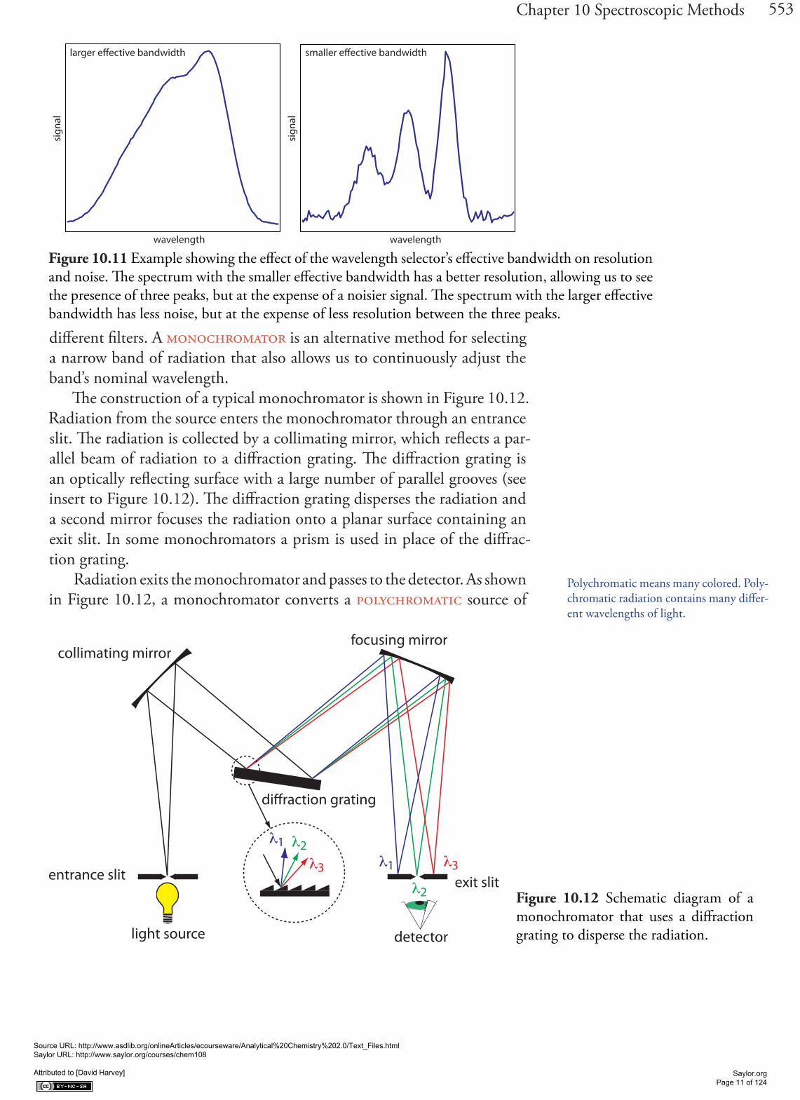
different filters. A monochromator is an alternative method for selecting a narrow band of radiation that also allows us to continuously adjust the band’s nominal wavelength.
The construction of a typical monochromator is shown in Figure 10.12. Radiation from the source enters the monochromator through an entrance slit. The radiation is collected by a collimating mirror, which reflects a par-allel beam of radiation to a diffraction grating. The diffraction grating is an optically reflecting surface with a large number of parallel grooves (see insert to Figure 10.12). The diffraction grating disperses the radiation and a second mirror focuses the radiation onto a planar surface containing an exit slit. In some monochromators a prism is used in place of the diffrac-tion grating.
Radiation exits the monochromator and passes to the detector. As shown in Figure 10.12, a monochromator converts a polychromatic source of
Figure 10.11 Example showing the effect of the wavelength selector’s effective bandwidth on resolution and noise. The spectrum with the smaller effective bandwidth has a better resolution, allowing us to see the presence of three peaks, but at the expense of a noisier signal. The spectrum with the larger effective bandwidth has less noise, but at the expense of less resolution between the three peaks.
Figure 10.12 Schematic diagram of a monochromator that uses a diffraction grating to disperse the radiation.
Polychromatic means many colored. Poly-chromatic radiation contains many differ-ent wavelengths of light.
wavelength
sign
al
wavelength
sign
al
larger effective bandwidth smaller effective bandwidth
λ1 λ3
λ2
λ1 λ2λ3entrance slit exit slit
collimating mirror
diffraction grating
focusing mirror
light source detector
Source URL: http://www.asdlib.org/onlineArticles/ecourseware/Analytical%20Chemistry%202.0/Text_Files.html Saylor URL: http://www.saylor.org/courses/chem108 Attributed to [David Harvey]
Saylor.org Page 11 of 124

554 Analytical Chemistry 2.0
radiation at the entrance slit to a monochromatic source of finite effective bandwidth at the exit slit. The choice of which wavelength exits the mono-chromator is determined by rotating the diffraction grating. A narrower exit slit provides a smaller effective bandwidth and better resolution, but allows a smaller throughput of radiation.
Monochromators are classified as either fixed-wavelength or scanning. In a fixed-wavelength monochromator we select the wavelength by manu-ally rotating the grating. Normally a fixed-wavelength monochromator is used for a quantitative analysis where measurements are made at one or two wavelengths. A scanning monochromator includes a drive mechanism that continuously rotates the grating, allowing successive wavelengths to exit from the monochromator. Scanning monochromators are used to acquire spectra, and, when operated in a fixed-wavelength mode, for a quantitative analysis.Interferometers. An interferometer provides an alternative approach for wavelength selection. Instead of filtering or dispersing the electromag-netic radiation, an interferometer allows source radiation of all wavelengths to reach the detector simultaneously (Figure 10.13). Radiation from the source is focused on a beam splitter that reflects half of the radiation to a fixed mirror and transmits the other half to a movable mirror. The radiation recombines at the beam splitter, where constructive and destructive inter-ference determines, for each wavelength, the intensity of light reaching the detector. As the moving mirror changes position, the wavelengths of light experiencing maximum constructive interference and maximum destruc-tive interference also changes. The signal at the detector shows intensity as a function of the moving mirror’s position, expressed in units of distance or time. The result is called an interferogram, or a time domain spectrum.
Monochromatic means one color, or one wavelength. Although the light exiting a monochromator is not strictly of a single wavelength, its narrow effective band-width allows us to think of it as mono-chromatic.
Figure 10.13 Schematic diagram of an inter-ferometers.
light source
detector
fixed mirror
moving mirrorbeam splitter
collimating mirror
focusing mirror
Source URL: http://www.asdlib.org/onlineArticles/ecourseware/Analytical%20Chemistry%202.0/Text_Files.html Saylor URL: http://www.saylor.org/courses/chem108 Attributed to [David Harvey]
Saylor.org Page 12 of 124

555Chapter 10 Spectroscopic Methods
The time domain spectrum is converted mathematically, by a process called a Fourier transform, to a spectrum (also called a frequency domain spec-trum) showing intensity as a function of the radiation’s energy.
In comparison to a monochromator, an interferometer has two sig-nificant advantages. The first advantage, which is termed jacquinot’s ad-vantage, is the higher throughput of source radiation. Because an inter-ferometer does not use slits and has fewer optical components from which radiation can be scattered and lost, the throughput of radiation reaching the detector is 80–200× greater than that for a monochromator. The result is less noise. The second advantage, which is called fellgett’s advantage, is a savings in the time needed to obtain a spectrum. Because the detector monitors all frequencies simultaneously, an entire spectrum takes approxi-mately one second to record, as compared to 10–15 minutes with a scan-ning monochromator.
DETECTORS
In Nessler’s original method for determining ammonia (Figure 10.9) the analyst’s eye serves as the detector, matching the sample’s color to that of a standard. The human eye, of course, has a poor range—responding only to visible light—nor is it particularly sensitive or accurate. Modern detectors use a sensitive transducer to convert a signal consisting of photons into an easily measured electrical signal. Ideally the detector’s signal, S, is a linear function of the electromagnetic radiation’s power, P,
S kP D= +
where k is the detector’s sensitivity, and D is the detector’s dark current, or the background current when we prevent the source’s radiation from reaching the detector.
There are two broad classes of spectroscopic transducers: thermal trans-ducers and photon transducers. Table 10.4 provides several representative examples of each class of transducers.
The mathematical details of the Fourier transform are beyond the level of this textbook. You can consult the chapter’s additional resources for additional infor-mation.
Transducer is a general term that refers to any device that converts a chemical or physical property into an easily measured electrical signal. The retina in your eye, for example, is a transducer that converts photons into an electrical nerve impulse.
Table 10.4 Examples of Transducers for SpectroscopyTransducer Class Wavelength Range Output Signalphototube photon 200–1000 nm currentphotomultiplier photon 110–1000 nm currentSi photodiode photon 250–1100 nm currentphotoconductor photon 750–6000 nm change in resistancephotovoltaic cell photon 400–5000 nm current or voltagethermocouple thermal 0.8–40 μm voltagethermistor thermal 0.8–40 μm change in resistancepneumatic thermal 0.8–1000 μm membrane displacementpyroelectric thermal 0.3–1000 μm current
Source URL: http://www.asdlib.org/onlineArticles/ecourseware/Analytical%20Chemistry%202.0/Text_Files.html Saylor URL: http://www.saylor.org/courses/chem108 Attributed to [David Harvey]
Saylor.org Page 13 of 124

556 Analytical Chemistry 2.0
Photon Transducers. Phototubes and photomultipliers contain a photo-sensitive surface that absorbs radiation in the ultraviolet, visible, or near IR, producing an electrical current proportional to the number of photons reaching the transducer (Figure 10.14). Other photon detectors use a semi-conductor as the photosensitive surface. When the semiconductor absorbs photons, valence electrons move to the semiconductor’s conduction band, producing a measurable current. One advantage of the Si photodiode is that it is easy to miniaturize. Groups of photodiodes may be gathered to-gether in a linear array containing from 64–4096 individual photodiodes. With a width of 25 μm per diode, for example, a linear array of 2048 pho-todiodes requires only 51.2 mm of linear space. By placing a photodiode array along the monochromator’s focal plane, it is possible to monitor simultaneously an entire range of wavelengths.Thermal Transducers. Infrared photons do not have enough energy to pro-duce a measurable current with a photon transducer. A thermal transducer, therefore, is used for infrared spectroscopy. The absorption of infrared pho-tons by a thermal transducer increases its temperature, changing one or more of its characteristic properties. A pneumatic transducer, for example, is a small tube of xenon gas with an IR transparent window at one end and a flexible membrane at the other end. Photons enter the tube and are absorbed by a blackened surface, increasing the temperature of the gas. As the temperature inside the tube fluctuates, the gas expands and contracts and the flexible membrane moves in and out. Monitoring the membrane’s displacement produces an electrical signal.
Signal Processors
A transducer’s electrical signal is sent to a signal processor where it is displayed in a form that is more convenient for the analyst. Examples of signal processors include analog or digital meters, recorders, and comput-ers equipped with digital acquisition boards. A signal processor also is used to calibrate the detector’s response, to amplify the transducer’s signal, to remove noise by filtering, or to mathematically transform the signal.
10B Spectroscopy Based on Absorption
In absorption spectroscopy a beam of electromagnetic radiation passes through a sample. Much of the radiation passes through the sample without a loss in intensity. At selected wavelengths, however, the radiation’s intensity is attenuated. This process of attenuation is called absorption.
10B.1 Absorbance Spectra
There are two general requirements for an analyte’s absorption of electro-magnetic radiation. First, there must be a mechanism by which the radia-tion’s electric field or magnetic field interacts with the analyte. For ultra-
Figure 10.14 Schematic of a photomulti-plier. A photon strikes the photoemissive cathode producing electrons, which ac-celerate toward a positively charged dyn-ode. Collision of these electrons with the dynode generates additional electrons, which accelerate toward the next dynode. A total of 106–107 electrons per photon eventually reach the anode, generating an electrical current.
If the retina in your eye is a transducer, then your brain is a signal processor.
hν
photoemissive cathode
dynode
anode
optical window
electrons
Source URL: http://www.asdlib.org/onlineArticles/ecourseware/Analytical%20Chemistry%202.0/Text_Files.html Saylor URL: http://www.saylor.org/courses/chem108 Attributed to [David Harvey]
Saylor.org Page 14 of 124

557Chapter 10 Spectroscopic Methods
violet and visible radiation, absorption of a photon changes the energy of the analyte’s valence electrons. A bond’s vibrational energy is altered by the absorption of infrared radiation.
The second requirement is that the photon’s energy, hν, must exactly equal the difference in energy, ΔE, between two of the analyte’s quantized energy states. Figure 10.4 shows a simplified view of a photon’s absorption, which is useful because it emphasizes that the photon’s energy must match the difference in energy between a lower-energy state and a higher-energy state. What is missing, however, is information about what types of energy states are involved, which transitions between energy states are likely to occur, and the appearance of the resulting spectrum.
We can use the energy level diagram in Figure 10.15 to explain an absor-bance spectrum. The lines labeled E0 and E1 represent the analyte’s ground (lowest) electronic state and its first electronic excited state. Superimposed on each electronic energy level is a series of lines representing vibrational energy levels.
INFRARED SPECTRA FOR MOLECULES AND POLYATOMIC IONS
The energy of infrared radiation produces a change in a molecule’s or a polyatomic ion’s vibrational energy, but is not sufficient to effect a change in its electronic energy. As shown in Figure 10.15, vibrational energy levels are quantized; that is, a molecule may have only certain, discrete vibrational energies. The energy for an allowed vibrational mode, Eν, is
E v hν ν= +12 0
Figure 10.3 provides a list of the types of atomic and molecular transitions associ-ated with different types of electromag-netic radiation.
Figure 10.15 Diagram showing two electronic energy levels (E0 and E1), each with five vibrational energy levels (ν0–ν4). Absorption of ultraviolet and visible radiation leads to a change in the analyte’s electronic energy levels and, possibly, a change in vibrational energy as well. A change in vibrational energy without a change in electronic energy levels occurs with the absorption of infrared radiation.
E0
E1
ν0
ν1
ν2
ν3
ν4
ν0
ν1
ν2
ν3
ν4
UV/Vis IR
ener
gy
Source URL: http://www.asdlib.org/onlineArticles/ecourseware/Analytical%20Chemistry%202.0/Text_Files.html Saylor URL: http://www.saylor.org/courses/chem108 Attributed to [David Harvey]
Saylor.org Page 15 of 124

558 Analytical Chemistry 2.0
where ν is the vibrational quantum number, which has values of 0, 1, 2, …, and ν0 is the bond’s fundamental vibrational frequency. The value of ν0, which is determined by the bond’s strength and by the mass at each end of the bond, is a characteristic property of a bond. For example, a carbon-carbon single bond (C–C) absorbs infrared radiation at a lower energy than a carbon-carbon double bond (C=C) because a single bond is weaker than a double bond.
At room temperature most molecules are in their ground vibrational state (ν = 0). A transition from the ground vibrational state to the first vibrational excited state (ν = 1) requires absorption of a photon with an energy of hν0. Transitions in which Δν is ±1 give rise to the fundamental absorption lines. Weaker absorption lines, called overtones, result from transitions in which Δν is ±2 or ±3. The number of possible normal vibra-tional modes for a linear molecule is 3N – 5, and for a non-linear molecule is 3N – 6, where N is the number of atoms in the molecule. Not surprisingly, infrared spectra often show a considerable number of absorption bands. Even a relatively simple molecule, such as ethanol (C2H6O), for example, has 3 × 9 – 6, or 21 possible normal modes of vibration, although not all of these vibrational modes give rise to an absorption. The IR spectrum for ethanol is shown in Figure 10.16.
UV/VIS SPECTRA FOR MOLECULES AND IONS
The valence electrons in organic molecules and polyatomic ions, such as CO3
2–, occupy quantized sigma bonding, σ, pi bonding, π, and non-bond-ing, n, molecular orbitals (MOs). Unoccupied sigma antibonding, σ*, and pi antibonding, π*, molecular orbitals are slightly higher in energy. Because the difference in energy between the highest-energy occupied MOs and
Figure 10.16 Infrared spectrum of ethanol.
Why does a non-linear molecule have 3N – 6 vibrational modes? Consider a molecule of methane, CH4. Each of the five atoms in methane can move in one of three directions (x, y, and z) for a total of 5 × 3 = 15 different ways in which the molecule can move. A molecule can move in three ways: it can move from one place to another, what we call translational mo-tion; it can rotate around an axis; and its bonds can stretch and bend, what we call vibrational motion.
Because the entire molecule can move in the x, y, and z directions, three of methane’s 15 different motions are translational. In addition, the molecule can rotate about its x, y, and z axes, accounting for three additional forms of motion. This leaves 15 – 3 – 3 = 9 vibrational modes.
A linear molecule, such as CO2, has 3N – 5 vibrational modes because it can rotate around only two axes.
4000 3000 2000 1000
0
20
40
60
80
100
wavenumber (cm-1)
perc
ent t
rans
mitt
ance
Source URL: http://www.asdlib.org/onlineArticles/ecourseware/Analytical%20Chemistry%202.0/Text_Files.html Saylor URL: http://www.saylor.org/courses/chem108 Attributed to [David Harvey]
Saylor.org Page 16 of 124

559Chapter 10 Spectroscopic Methods
the lowest-energy unoccupied MOs corresponds to ultraviolet and visible radiation, absorption of a photon is possible.
Four types of transitions between quantized energy levels account for most molecular UV/Vis spectra. Table 10.5 lists the approximate wave-length ranges for these transitions, as well as a partial list of bonds, func-tional groups, or molecules responsible for these transitions. Of these tran-sitions, the most important are n→ ∗π and π π→ ∗ because they involve important functional groups that are characteristic of many analytes and because the wavelengths are easily accessible. The bonds and functional groups that give rise to the absorption of ultraviolet and visible radiation are called chromophores.
Many transition metal ions, such as Cu2+ and Co2+, form colorful solu-tions because the metal ion absorbs visible light. The transitions giving rise to this absorption are valence electrons in the metal ion’s d-orbitals. For a free metal ion, the five d-orbitals are of equal energy. In the presence of a complexing ligand or solvent molecule, however, the d-orbitals split into two or more groups that differ in energy. For example, in an octahedral complex of Cu(H2O)6
2+ the six water molecules perturb the d-orbitals into two groups, as shown in Figure 10.17. The resulting d–d transitions for transition metal ions are relatively weak.
A more important source of UV/Vis absorption for inorganic metal–ligand complexes is charge transfer, in which absorption of a photon pro-duces an excited state in which there is transfer of an electron from the metal, M, to the ligand, L.
M—L + hν é (M+—L–)*
Charge-transfer absorption is important because it produces very large ab-sorbances. One important example of a charge-transfer complex is that of o-phenanthroline with Fe2+, the UV/Vis spectrum for which is shown in Figure 10.18. Charge-transfer absorption in which an electron moves from the ligand to the metal also is possible.
Comparing the IR spectrum in Figure 10.16 to the UV/Vis spectrum in Figure 10.18 shows us that UV/Vis absorption bands are often significantly broader than those for IR absorption. We can use Figure 10.15 to explain
Table 10.5 Electronic Transitions Involving n, σ, and π Molecular Orbitals
Transition Wavelength Range Examples
σ σ→ ∗ <200 nm C–C, C–H
n→ ∗σ 160–260 nm H2O, CH3OH, CH3Cl
π π→ ∗ 200–500 nm C=C, C=O, C=N, C≡C
n→ ∗π 250–600 nm C=O, C=N, N=N, N=O
Figure 10.17 Splitting of the d-orbitals in an octahedral field.
Why is a larger absorbance desirable? An analytical method is more sensitive if a smaller concentration of analyte gives a larger signal.
dx2–y2dz2
dxy dxz dyz
hν
Source URL: http://www.asdlib.org/onlineArticles/ecourseware/Analytical%20Chemistry%202.0/Text_Files.html Saylor URL: http://www.saylor.org/courses/chem108 Attributed to [David Harvey]
Saylor.org Page 17 of 124

560 Analytical Chemistry 2.0
why this is true. When a species absorbs UV/Vis radiation, the transition between electronic energy levels may also include a transition between vi-brational energy levels. The result is a number of closely spaced absorption bands that merge together to form a single broad absorption band.
UV/VIS SPECTRA FOR ATOMS
The energy of ultraviolet and visible electromagnetic radiation is sufficient to cause a change in an atom’s valence electron configuration. Sodium, for example, has a single valence electron in its 3s atomic orbital. As shown in Figure 10.19, unoccupied, higher energy atomic orbitals also exist.
Absorption of a photon is accompanied by the excitation of an electron from a lower-energy atomic orbital to an orbital of higher energy. Not all possible transitions between atomic orbitals are allowed. For sodium the only allowed transitions are those in which there is a change of ±1 in the orbital quantum number (l); thus transitions from s é p orbitals are allowed, and transitions from s é d orbitals are forbidden.
Figure 10.18 UV/Vis spectrum for the metal–ligand complex Fe(phen)3
2+, where phen is the ligand o-phenanthroline.
Figure 10.19 Valence shell energy level diagram for so-dium. The wavelengths (in wavenumbers) correspond-ing to several transitions are shown.
The valence shell energy level diagram in Figure 10.19 might strike you as odd because it shows that the 3p orbitals are split into two groups of slightly different energy. The reasons for this splitting are unimportant in the context of our treat-ment of atomic absorption. For further information about the reasons for this splitting, consult the chapter’s additional resources.
400 450 500 550 600 650 700
0.0
0.2
0.4
0.6
0.8
1.0
1.2
wavelength (nm)
abso
rban
ce
1138.3
589.6 589.0
819.5
818.3330.2
330.3
1140.4
3s
3p
3d
4s
4p
4d
5s
5p
Ener
gy
Source URL: http://www.asdlib.org/onlineArticles/ecourseware/Analytical%20Chemistry%202.0/Text_Files.html Saylor URL: http://www.saylor.org/courses/chem108 Attributed to [David Harvey]
Saylor.org Page 18 of 124

561Chapter 10 Spectroscopic Methods
The atomic absorption spectrum for Na is shown in Figure 10.20, and is typical of that found for most atoms. The most obvious feature of this spectrum is that it consists of a small number of discrete absorption lines corresponding to transitions between the ground state (the 3s atomic or-bital) and the 3p and 4p atomic orbitals. Absorption from excited states, such as the 3p é 4s and the 3p é 3d transitions included in Figure 10.19, are too weak to detect. Because an excited state’s lifetime is short—typically an excited state atom takes 10–7 to 10–8 s to return to a lower energy state—an atom in the exited state is likely to return to the ground state before it has an opportunity to absorb a photon.
Another feature of the atomic absorption spectrum in Figure 10.20 is the narrow width of the absorption lines, which is a consequence of the fixed difference in energy between the ground and excited states. Natural line widths for atomic absorption, which are governed by the uncertainty principle, are approximately 10–5 nm. Other contributions to broadening increase this line width to approximately 10–3 nm.
10B.2 Transmittance and Absorbance
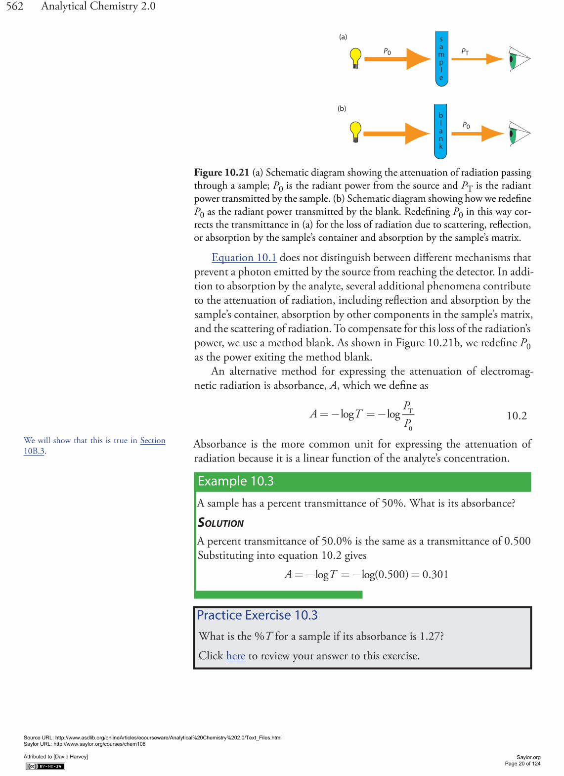
As light passes through a sample, its power decreases as some of it is ab-sorbed. This attenuation of radiation is described quantitatively by two separate, but related terms: transmittance and absorbance. As shown in Figure 10.21a, transmittance is the ratio of the source radiation’s power exiting the sample, PT, to that incident on the sample, P0.
TPP
= T
0
10.1
Multiplying the transmittance by 100 gives the percent transmittance, %T, which varies between 100% (no absorption) and 0% (complete absorp-tion). All methods of detecting photons—including the human eye and modern photoelectric transducers—measure the transmittance of electro-magnetic radiation.
Figure 10.20 Atomic absorption spectrum for sodium. Note that the scale on the x-axis includes a break.
588.5 589.0 589.5330.0 330.2 330.4
wavelength (nm)
590.0
1.0
0.8
0.6
0.4
0.2
0
abso
rban
ce
3s 4p
3s 3p
Source URL: http://www.asdlib.org/onlineArticles/ecourseware/Analytical%20Chemistry%202.0/Text_Files.html Saylor URL: http://www.saylor.org/courses/chem108 Attributed to [David Harvey]
Saylor.org Page 19 of 124
562 Analytical Chemistry 2.0
Equation 10.1 does not distinguish between different mechanisms that prevent a photon emitted by the source from reaching the detector. In addi-tion to absorption by the analyte, several additional phenomena contribute to the attenuation of radiation, including reflection and absorption by the sample’s container, absorption by other components in the sample’s matrix, and the scattering of radiation. To compensate for this loss of the radiation’s power, we use a method blank. As shown in Figure 10.21b, we redefine P0 as the power exiting the method blank.
An alternative method for expressing the attenuation of electromag-netic radiation is absorbance, A, which we define as
A TPP
=− =−log log T
0
10.2
Absorbance is the more common unit for expressing the attenuation of radiation because it is a linear function of the analyte’s concentration.
Example 10.3
A sample has a percent transmittance of 50%. What is its absorbance?
SOLUTION
A percent transmittance of 50.0% is the same as a transmittance of 0.500 Substituting into equation 10.2 gives
A T=− =− =log log( . ) .0 500 0 301
Figure 10.21 (a) Schematic diagram showing the attenuation of radiation passing through a sample; P0 is the radiant power from the source and PT is the radiant power transmitted by the sample. (b) Schematic diagram showing how we redefine P0 as the radiant power transmitted by the blank. Redefining P0 in this way cor-rects the transmittance in (a) for the loss of radiation due to scattering, reflection, or absorption by the sample’s container and absorption by the sample’s matrix.
We will show that this is true in Section 10B.3.
Practice Exercise 10.3What is the %T for a sample if its absorbance is 1.27?
Click here to review your answer to this exercise.
P0
(b)
P0 PT
(a)
Source URL: http://www.asdlib.org/onlineArticles/ecourseware/Analytical%20Chemistry%202.0/Text_Files.html Saylor URL: http://www.saylor.org/courses/chem108 Attributed to [David Harvey]
Saylor.org Page 20 of 124

563Chapter 10 Spectroscopic Methods
Equation 10.1 has an important consequence for atomic absorption. As we saw in Figure 10.20, atomic absorption lines are very narrow. Even with a high quality monochromator, the effective bandwidth for a continuum source is 100–1000× greater than the width of an atomic absorption line. As a result, little of the radiation from a continuum source is absorbed (P0 ≈ PT), and the measured absorbance is effectively zero. For this reason, atomic absorption requires a line source instead of a continuum source.
10B.3 Absorbance and Concentration: Beer’s Law
When monochromatic electromagnetic radiation passes through an infini-tesimally thin layer of sample of thickness dx, it experiences a decrease in its power of dP (Figure 10.22). The fractional decrease in power is propor-tional to the sample’s thickness and the analyte’s concentration, C; thus
− =dPP
Cdxα 10.3
where P is the power incident on the thin layer of sample, and α is a pro-portionality constant. Integrating the left side of equation 10.3 over the entire sample
− =∫ ∫dPP
C dxP
P
o
b
0
Tα
lnPP
bC0
T
=α
converting from ln to log, and substituting in equation 10.2, givesA abC= 10.4
where a is the analyte’s absorptivity with units of cm–1 conc–1. If we ex-press the concentration using molarity, then we replace a with the molar absorptivity, ε, which has units of cm–1 M–1.
A bC= ε 10.5The absorptivity and molar absorptivity are proportional to the probability that the analyte absorbs a photon of a given energy. As a result, values for both a and ε depend on the wavelength of the absorbed photon.
Figure 10.22 Factors used in deriving the Beer-Lambert law.dxx = 0 x = b
P0 P P – dP PT
Source URL: http://www.asdlib.org/onlineArticles/ecourseware/Analytical%20Chemistry%202.0/Text_Files.html Saylor URL: http://www.saylor.org/courses/chem108 Attributed to [David Harvey]
Saylor.org Page 21 of 124

564 Analytical Chemistry 2.0
Example 10.4
A 5.00 × 10⁻⁴ M solution of an analyte is placed in a sample cell with a pathlength of 1.00 cm. When measured at a wavelength of 490 nm, the solution’s absorbance is 0.338. What is the analyte’s molar absorptivity at this wavelength?
SOLUTION
Solving equation 10.5 for ε and making appropriate substitutions gives
ε= =×
=−
−AbC
0 3381 00 10
6764
1.( . cm)(5.00 M)
cm MM−1
Practice Exercise 10.4A solution of the analyte from Example 10.4 has an absorbance of 0.228 in a 1.00-cm sample cell. What is the analyte’s concentration?
Click here to review your answer to this exercise.
Equation 10.4 and equation 10.5, which establish the linear relation-ship between absorbance and concentration, are known as the Beer-Lam-bert law, or more commonly, as beer’s law. Calibration curves based on Beer’s law are common in quantitative analyses.
10B.4 Beer’s Law and Multicomponent Samples
We can extend Beer’s law to a sample containing several absorbing compo-nents. If there are no interactions between the components, the individual absorbances, Ai, are additive. For a two-component mixture of analyte’s X and Y, the total absorbance, Atot, is
A A A bC bCtot X Y X X Y Y= + = +ε ε
Generalizing, the absorbance for a mixture of n components, Amix, is
A A bCii
n
i ii
n
mix = == =∑ ∑
1 1
ε 10.6
10B.5 Limitations to Beer’s Law
Beer’s law suggests that a calibration curve is a straight line with a y-inter-cept of zero and a slope of ab or εb. In many cases a calibration curve devi-ates from this ideal behavior (Figure 10.23). Deviations from linearity are divided into three categories: fundamental, chemical, and instrumental.
FUNDAMENTAL LIMITATIONS TO BEER’S LAW
Beer’s law is a limiting law that is valid only for low concentrations of analyte. There are two contributions to this fundamental limitation to Beer’s law. At
Figure 10.23 Calibration curves show-ing positive and negative deviations from the ideal Beer’s law calibration curve, which is a straight line.
ideal
negativedeviation
positivedeviation
concentration
abso
rban
ce
Source URL: http://www.asdlib.org/onlineArticles/ecourseware/Analytical%20Chemistry%202.0/Text_Files.html Saylor URL: http://www.saylor.org/courses/chem108 Attributed to [David Harvey]
Saylor.org Page 22 of 124

565Chapter 10 Spectroscopic Methods
higher concentrations the individual particles of analyte no longer behave independently of each other. The resulting interaction between particles of analyte may change the analyte’s absorptivity. A second contribution is that the analyte’s absorptivity depends on the sample’s refractive index. Because the refractive index varies with the analyte’s concentration, the values of a and ε may change. For sufficiently low concentrations of analyte, the refrac-tive index is essentially constant and the calibration curve is linear.
CHEMICAL LIMITATIONS TO BEER’S LAW
A chemical deviation from Beer’s law may occur if the analyte is involved in an equilibrium reaction. Consider, as an example, an analysis for the weak acid, HA. To construct a Beer’s law calibration curve we prepare a series of standards—each containing a known total concentration of HA—and measure each standard’s absorbance at the same wavelength. Because HA is a weak acid, it is in equilibrium with its conjugate weak base, A–.
HA H O H O A2 3( ) ( ) ( ) ( )aq l aq aq+ ++ −É
If both HA and A– absorb at the chosen wavelength, then Beer’s law is
A bC bC= +ε εHA HA A A 10.7
where CHA and CA are the equilibrium concentrations of HA and A–. Be-cause the weak acid’s total concentration, Ctotal, is
C C Ctotal HA A= +
the concentrations of HA and A– can be written as
C CHA HA total=α 10.8
C CA HA total= −( )1 α 10.9
where αHA is the fraction of weak acid present as HA. Substituting equation 10.8 and equation 10.9 into equation 10.7 and rearranging, gives
A bC= + −( )ε α ε ε αHA HA A A HA total 10.10
To obtain a linear Beer’s law calibration curve, one of two conditions must be met. If αHA and αA have the same value at the chosen wavelength, then equation 10.10 simplifies to
A bC= εA total
Alternatively, if αHA has the same value for all standards, then each term within the parentheses of equation 10.10 is constant—which we replace with k—and a linear calibration curve is obtained at any wavelength.
A kbC= total
Source URL: http://www.asdlib.org/onlineArticles/ecourseware/Analytical%20Chemistry%202.0/Text_Files.html Saylor URL: http://www.saylor.org/courses/chem108 Attributed to [David Harvey]
Saylor.org Page 23 of 124

566 Analytical Chemistry 2.0
Because HA is a weak acid, the value of αHA varies with pH. To hold αHA constant we buffer each standard to the same pH. Depending on the relative values of αHA and αA, the calibration curve has a positive or a negative deviation from Beer’s law if we do not buffer the standards to the same pH.
INSTRUMENTAL LIMITATIONS TO BEER’S LAW
There are two principal instrumental limitations to Beer’s law. The first limi-tation is that Beer’s law assumes that the radiation reaching the sample is of a single wavelength—that is, that the radiation is purely monochromatic. As shown in Figure 10.10, however, even the best wavelength selector passes radiation with a small, but finite effective bandwidth. Polychromatic ra-diation always gives a negative deviation from Beer’s law, but the effect is smaller if the value of ε is essentially constant over the wavelength range passed by the wavelength selector. For this reason, as shown in Figure 10.24, it is better to make absorbance measurements at the top of a broad absorp-tion peak. In addition, the deviation from Beer’s law is less serious if the source’s effective bandwidth is less than one-tenth of the natural bandwidth of the absorbing species.5 When measurements must be made on a slope, linearity is improved by using a narrower effective bandwidth.
Stray radiation is the second contribution to instrumental deviations from Beer’s law. Stray radiation arises from imperfections in the wavelength selector that allow light to enter the instrument and reach the detector without passing through the sample. Stray radiation adds an additional contribution, Pstray, to the radiant power reaching the detector; thus
AP P
P P=−
+
+log T stray
0 stray
For a small concentration of analyte, Pstray is significantly smaller than P0 and PT, and the absorbance is unaffected by the stray radiation. At a higher concentration of analyte, however, less light passes through the sample and
5 (a) Strong, F. C., III Anal. Chem. 1984, 56, 16A–34A; Gilbert, D. D. J. Chem. Educ. 1991, 68, A278–A281.
For a monoprotic weak acid, the equation for αHA is
αHA3
3 a
H O
H O=
+
+
+
[ ]
[ ] K
Problem 10.6 in the end of chapter prob-lems asks you to explore this chemical limitation to Beer’s law.
Figure 10.24 Effect of the choice of wavelength on the linearity of a Beer’s law calibration curve.
Another reason for measuring absorbance at the top of an absorbance peak is that it provides for a more sensitive analysis. Note that the green calibration curve in Figure 10.24 has a steeper slope—a greater sensitivity—than the red calibra-tion curve.
Problem 10.7 in the end of chapter prob-lems ask you to explore the effect of poly-chromatic radiation on the linearity of Beer’s law.
400 450 500 550 600 650 700
0.0
0.2
0.4
0.6
0.8
1.0
1.2
wavelength (nm)
abso
rban
ce
concentration
abso
rban
ce
Source URL: http://www.asdlib.org/onlineArticles/ecourseware/Analytical%20Chemistry%202.0/Text_Files.html Saylor URL: http://www.saylor.org/courses/chem108 Attributed to [David Harvey]
Saylor.org Page 24 of 124

567Chapter 10 Spectroscopic Methods
PT and Pstray may be similar in magnitude. This results is an absorbance that is smaller than expected, and a negative deviation from Beer’s law.
10C UV/Vis and IR Spectroscopy
In Figure 10.9 we examined Nessler’s original method for matching the color of a sample to the color of a standard. Matching the colors was a labor intensive process for the analyst. Not surprisingly, spectroscopic methods of analysis were slow to develop. The 1930s and 1940s saw the introduction of photoelectric transducers for ultraviolet and visible radiation, and ther-mocouples for infrared radiation. As a result, modern instrumentation for absorption spectroscopy became routinely available in the 1940s—progress has been rapid ever since.
10C.1 Instrumentation
Frequently an analyst must select—from among several instruments of dif-ferent design—the one instrument best suited for a particular analysis. In this section we examine several different instruments for molecular absorp-tion spectroscopy, emphasizing their advantages and limitations. Methods of sample introduction are also covered in this section.
INSTRUMENT DESIGNS FOR MOLECULAR UV/VIS ABSORPTION
Filter Photometer. The simplest instrument for molecular UV/Vis absorp-tion is a filter photometer (Figure 10.25), which uses an absorption or interference filter to isolate a band of radiation. The filter is placed between the source and the sample to prevent the sample from decomposing when exposed to higher energy radiation. A filter photometer has a single optical path between the source and detector, and is called a single-beam instru-ment. The instrument is calibrated to 0% T while using a shutter to block the source radiation from the detector. After opening the shutter, the in-
Problem 10.8 in the end of chapter prob-lems ask you to explore the effect of stray radiation on the linearity of Beer’s law.
Figure 10.25 Schematic diagram of a filter photom-eter. The analyst either inserts a removable filter or the filters are placed in a carousel, an example of which is shown in the photographic inset. The analyst selects a filter by rotating it into place.
The percent transmittance varies between 0% and 100%. As we learned in Figure 10.21, we use a blank to determine P0, which corresponds to 100% T. Even in the absence of light the detector records a sig-nal. Closing the shutter allows us to assign 0% T to this signal. Together, setting 0% T and 100% T calibrates the instrument. The amount of light passing through a sample produces a signal that is greater than or equal to that for 0% T and smaller than or equal to that for 100%T.
open
closedsource
detectorfilter shutter
signalprocessor
Source URL: http://www.asdlib.org/onlineArticles/ecourseware/Analytical%20Chemistry%202.0/Text_Files.html Saylor URL: http://www.saylor.org/courses/chem108 Attributed to [David Harvey]
Saylor.org Page 25 of 124

568 Analytical Chemistry 2.0
strument is calibrated to 100% T using an appropriate blank. The blank is then replaced with the sample and its transmittance measured. Because the source’s incident power and the sensitivity of the detector vary with wave-length, the photometer must be recalibrated whenever the filter is changed. Photometers have the advantage of being relatively inexpensive, rugged, and easy to maintain. Another advantage of a photometer is its portability, making it easy to take into the field. Disadvantages of a photometer include the inability to record an absorption spectrum and the source’s relatively large effective bandwidth, which limits the calibration curve’s linearity. Single-Beam Spectrophotometer. An instrument that uses a monochro-mator for wavelength selection is called a spectrophotometer. The simplest spectrophotometer is a single-beam instrument equipped with a fixed-wavelength monochromator (Figure 10.26). Single-beam spectro-photometers are calibrated and used in the same manner as a photometer. One example of a single-beam spectrophotometer is Thermo Scientific’s Spectronic 20D+, which is shown in the photographic insert to Figure 10.26. The Spectronic 20D+ has a range of 340–625 nm (950 nm when using a red-sensitive detector), and a fixed effective bandwidth of 20 nm. Battery-operated, hand-held single-beam spectrophotometers are available, which are easy to transport into the field. Other single-beam spectropho-tometers also are available with effective bandwidths of 2–8 nm. Fixed wavelength single-beam spectrophotometers are not practical for recording spectra because manually adjusting the wavelength and recalibrating the spectrophotometer is awkward and time-consuming. The accuracy of a single-beam spectrophotometer is limited by the stability of its source and detector over time.Double-Beam Spectrophotometer. The limitations of fixed-wavelength, single-beam spectrophotometers are minimized by using a double-beam spectrophotometer (Figure 10.27). A chopper controls the radiation’s path,
Figure 10.26 Schematic diagram of a fixed-wavelength single-beam spectrophotometer. The photographic in-set shows a typical instrument. The shutter remains closed until the sample or blank is placed in the sample compartment. The analyst manually selects the wave-length by adjusting the wavelength dial. Inset photo modified from: Adi (www.commons.wikipedia.org).
λ1 λ2λ3
open
closed
shuttersource
monochromator
detector
signalprocessor
wavelengthdial
samplecompartment
0% T and 100% Tadjustment
P0
PT
Source URL: http://www.asdlib.org/onlineArticles/ecourseware/Analytical%20Chemistry%202.0/Text_Files.html Saylor URL: http://www.saylor.org/courses/chem108 Attributed to [David Harvey]
Saylor.org Page 26 of 124

569Chapter 10 Spectroscopic Methods
alternating it between the sample, the blank, and a shutter. The signal processor uses the chopper’s known speed of rotation to resolve the signal reaching the detector into the transmission of the blank, P0, and the sample, PT. By including an opaque surface as a shutter, it is possible to continu-ously adjust 0% T. The effective bandwidth of a double-beam spectropho-tometer is controlled by adjusting the monochromator’s entrance and exit slits. Effective bandwidths of 0.2–3.0 nm are common. A scanning mono-chromator allows for the automated recording of spectra. Double-beam instruments are more versatile than single-beam instruments, being useful for both quantitative and qualitative analyses, but also are more expensive.Diode Array Spectrometer. An instrument with a single detector can monitor only one wavelength at a time. If we replace a single photomul-tiplier with many photodiodes, we can use the resulting array of detectors to record an entire spectrum simultaneously in as little as 0.1 s. In a diode array spectrometer the source radiation passes through the sample and is dispersed by a grating (Figure 10.28). The photodiode array is situated at the grating’s focal plane, with each diode recording the radiant power over a narrow range of wavelengths. Because we replace a full monochromator with just a grating, a diode array spectrometer is small and compact.
Figure 10.27 Schematic diagram of a scanning, double-beam spectrophotometer. A chopper directs the source’s radiation, using a transparent window to pass radiation to the sample and a mirror to reflect radiation to the blank. The chopper’s opaque surface serves as a shutter, which allows for a constant adjustment of the spectro-photometer’s 0% T. The photographic insert shows a typical instrument. The unit in the middle of the photo is a temperature control unit that allows the sample to be heated or cooled.
λ1 λ2λ3
source
monochromator
detector
signalprocessor
chopper
mirror
mirror
semitransparentmirror
sample
blank
shutter
samplecompartment
temperaturecontrol
P0
PT
Source URL: http://www.asdlib.org/onlineArticles/ecourseware/Analytical%20Chemistry%202.0/Text_Files.html Saylor URL: http://www.saylor.org/courses/chem108 Attributed to [David Harvey]
Saylor.org Page 27 of 124

570 Analytical Chemistry 2.0
One advantage of a diode array spectrometer is the speed of data acqui-sition, which allows to collect several spectra for a single sample. Individual spectra are added and averaged to obtain the final spectrum. This signal averaging improves a spectrum’s signal-to-noise ratio. If we add together n spectra, the sum of the signal at any point, x, increases as nSx, where Sx is the signal. The noise at any point, Nx, is a random event, which increases as
nN x when we add together n spectra. The signal-to-noise ratio (S/N) after n scans is
SN
nS
nNn
SN
x
x
x
x
= =
where Sx/Nx is the signal-to-noise ratio for a single scan. The impact of sig-nal averaging is shown in Figure 10.29. The first spectrum shows the signal for a single scan, which consists of a single, noisy peak. Signal averaging using 4 scans and 16 scans decreases the noise and improves the signal-to-noise ratio. One disadvantage of a photodiode array is that the effective bandwidth per diode is roughly an order of magnitude larger than that for a high quality monochromator.Sample Cells. The sample compartment provides a light-tight environment that limits the addition of stray radiation. Samples are normally in the liquid or solution state, and are placed in cells constructed with UV/Vis transparent materials, such as quartz, glass, and plastic (Figure 10.30). A quartz or fused-silica cell is required when working at a wavelength <300 nm where other materials show a significant absorption. The most common pathlength is 1 cm (10 mm), although cells with shorter (as little as 0.1 cm) and longer pathlengths (up to 10 cm) are available. Longer pathlength cells
Figure 10.29 Effect of signal averaging on a spectrum’s signal-to-noise ratio. From top to bottom: spectrum for a single scan; average spectrum after four scans; and average spectrum after adding 16 scans.
λ1 λ2λ3
open
closed
shuttersource
grating
detectors
signalprocessorsample
compartment
P0
PTFigure 10.28 Schematic diagram of a diode array spectrophotometer. The photographic in-sert shows a typical instrument. Note that the 50-mL beaker provides a sense of scale.
500 550 600 650 700
wavelength
1.0
0.8
0.6
0.4
0.2
0
abso
rban
ce
1 scan
500 550 600 650 700
wavelength
1.0
0.8
0.6
0.4
0.2
0
abso
rban
ce
4 scans
500 550 600 650 700
wavelength
1.0
0.8
0.6
0.4
0.2
0
abso
rban
ce
16 scans
Source URL: http://www.asdlib.org/onlineArticles/ecourseware/Analytical%20Chemistry%202.0/Text_Files.html Saylor URL: http://www.saylor.org/courses/chem108 Attributed to [David Harvey]
Saylor.org Page 28 of 124

571Chapter 10 Spectroscopic Methods
are useful when analyzing a very dilute solution, or for gas samples. The highest quality cells allow the radiation to strike a flat surface at a 90o angle, minimizing the loss of radiation to reflection. A test tube is often used as a sample cell with simple, single-beam instruments, although differences in the cell’s pathlength and optical properties add an additional source of error to the analysis.
If we need to monitor an analyte’s concentration over time, it may not be possible to physically remove samples for analysis. This is often the case, for example, when monitoring industrial production lines or waste lines, when monitoring a patient’s blood, or when monitoring environmental systems. With a fiber-optic probe we can analyze samples in situ. An ex-ample of a remote sensing fiber-optic probe is shown in Figure 10.31. The probe consists of two bundles of fiber-optic cable. One bundle transmits radiation from the source to the probe’s tip, which is designed to allow the sample to flow through the sample cell. Radiation from the source passes through the solution and is reflected back by a mirror. The second bundle
Figure 10.30 Examples of sample cells for UV/Vis spectroscopy. From left to right (with path lengths in pa-rentheses): rectangular plastic cuvette (10.0 mm), rectangular quartz cuvette (5.000 mm), rectangular quartz cuvette (1.000 mm), cylindrical quartz cuvette (10.00 mm), cylindrical quartz cuvette (100.0 mm). Cells often are available as a matched pair, which is important when using a double-beam instrument.
Figure 10.31 Example of a fiber-optic probe. The inset photographs provide a close-up look at the probe’s flow cell and the reflecting mirror
light in light out
probe’s tip
reflectingmirror
flow cell
Source URL: http://www.asdlib.org/onlineArticles/ecourseware/Analytical%20Chemistry%202.0/Text_Files.html Saylor URL: http://www.saylor.org/courses/chem108 Attributed to [David Harvey]
Saylor.org Page 29 of 124

572 Analytical Chemistry 2.0
of fiber-optic cable transmits the nonabsorbed radiation to the wavelength selector. Another design replaces the flow cell shown in Figure 10.31 with a membrane containing a reagent that reacts with the analyte. When the analyte diffuses across the membrane it reacts with the reagent, producing a product that absorbs UV or visible radiation. The nonabsorbed radiation from the source is reflected or scattered back to the detector. Fiber optic probes that show chemical selectivity are called optrodes.6
INSTRUMENT DESIGNS FOR INFRARED ABSORPTION
Filter Photometer. The simplest instrument for IR absorption spectroscopy is a filter photometer similar to that shown in Figure 10.25 for UV/Vis ab-sorption. These instruments have the advantage of portability, and typically are used as dedicated analyzers for gases such as HCN and CO.Double-beam spectrophotometer. Infrared instruments using a mono-chromator for wavelength selection use double-beam optics similar to that shown in Figure 10.27. Double-beam optics are preferred over single-beam optics because the sources and detectors for infrared radiation are less stable than those for UV/Vis radiation. In addition, it is easier to correct for the absorption of infrared radiation by atmospheric CO2 and H2O vapor when using double-beam optics. Resolutions of 1–3 cm–1 are typical for most instruments.Fourier transform spectrometer. In a Fourier transform infrared spectrom-eter, or FT–IR, the monochromator is replaced with an interferometer (Figure 10.13). Because an FT-IR includes only a single optical path, it is necessary to collect a separate spectrum to compensate for the absor-bance of atmospheric CO2 and H2O vapor. This is done by collecting a background spectrum without the sample and storing the result in the in-strument’s computer memory. The background spectrum is removed from the sample’s spectrum by ratioing the two signals. In comparison to other instrument designs, an FT–IR provides for rapid data acquisition, allowing an enhancement in signal-to-noise ratio through signal-averaging. Sample Cells. Infrared spectroscopy is routinely used to analyze gas, liquid, and solid samples. Sample cells are made from materials, such as NaCl and KBr, that are transparent to infrared radiation. Gases are analyzed using a cell with a pathlength of approximately 10 cm. Longer pathlengths are obtained by using mirrors to pass the beam of radiation through the sample several times.
A liquid samples may be analyzed using a variety of different sample cells (Figure 10.32). For non-volatile liquids a suitable sample can be pre-pared by placing a drop of the liquid between two NaCl plates, forming a thin film that typically is less than 0.01 mm thick. Volatile liquids must be placed in a sealed cell to prevent their evaporation.
6 (a) Seitz, W. R. Anal. Chem. 1984, 56, 16A–34A; (b) Angel, S. M. Spectroscopy 1987, 2(2), 38–48.
Source URL: http://www.asdlib.org/onlineArticles/ecourseware/Analytical%20Chemistry%202.0/Text_Files.html Saylor URL: http://www.saylor.org/courses/chem108 Attributed to [David Harvey]
Saylor.org Page 30 of 124

573Chapter 10 Spectroscopic Methods
The analysis of solution samples is limited by the solvent’s IR absorbing properties, with CCl4, CS2, and CHCl3 being the most common solvents. Solutions are placed in cells containing two NaCl windows separated by a Teflon spacer. By changing the Teflon spacer, pathlengths from 0.015–1.0 mm can be obtained.
Transparent solid samples can be analyzed directly by placing them in the IR beam. Most solid samples, however, are opaque, and must be dis-persed in a more transparent medium before recording the IR spectrum. If a suitable solvent is available, then the solid can be analyzed by preparing a solution and analyzing as described above. When a suitable solvent is not available, solid samples may be analyzed by preparing a mull of the finely powdered sample with a suitable oil. Alternatively, the powdered sample can be mixed with KBr and pressed into an optically transparent pellet.
The analysis of an aqueous sample is complicated by the solubility of the NaCl cell window in water. One approach to obtaining infrared spectra on aqueous solutions is to use attenuated total reflectance instead of transmission. Figure 10.33 shows a diagram of a typical attenuated total reflectance (ATR) FT–IR instrument. The ATR cell consists of a high re-fractive index material, such as ZnSe or diamond, sandwiched between a low refractive index substrate and a lower refractive index sample. Radia-tion from the source enters the ATR crystal where it undergoes a series of total internal reflections before exiting the crystal. During each reflection the radiation penetrates into the sample to a depth of a few microns. The result is a selective attenuation of the radiation at those wavelengths where
Figure 10.32 Three examples of IR sample cells: (a) NaCl salts plates; (b) fixed pathlength (0.5 mm) sample cell with NaCl windows; (c) disposable card with a polyethylene window that is IR transparent with the exception of strong ab-sorption bands at 2918 cm–1 and 2849 cm–1.
(a) (b) (c)
Source URL: http://www.asdlib.org/onlineArticles/ecourseware/Analytical%20Chemistry%202.0/Text_Files.html Saylor URL: http://www.saylor.org/courses/chem108 Attributed to [David Harvey]
Saylor.org Page 31 of 124

574 Analytical Chemistry 2.0
the sample absorbs. ATR spectra are similar, but not identical, to those obtained by measuring the transmission of radiation.
Solid samples also can be analyzed using an ATR sample cell. After placing the solid in the sample slot, a compression tip ensures that it is in contact with the ATR crystal. Examples of solids that have been analyzed by ATR include polymers, fibers, fabrics, powders, and biological tissue samples. Another reflectance method is diffuse reflectance, in which radia-tion is reflected from a rough surface, such as a powder. Powdered samples are mixed with a non-absorbing material, such as powdered KBr, and the reflected light is collected and analyzed. As with ATR, the resulting spec-trum is similar to that obtained by conventional transmission methods.
10C.2 Quantitative Applications
The determination of an analyte’s concentration based on its absorption of ultraviolet or visible radiation is one of the most frequently encountered quantitative analytical methods. One reason for its popularity is that many organic and inorganic compounds have strong absorption bands in the UV/Vis region of the electromagnetic spectrum. In addition, if an analyte does not absorb UV/Vis radiation—or if its absorbance is too weak—we often can react it with another species that is strongly absorbing. For example, a dilute solution of Fe2+ does not absorb visible light. Reacting Fe2+ with o-phenanthroline, however, forms an orange–red complex of Fe(phen)3
2+ that has a strong, broad absorbance band near 500 nm. An additional advantage to UV/Vis absorption is that in most cases it is relatively easy to adjust ex-perimental and instrumental conditions so that Beer’s law is obeyed.
Figure 10.33 FT-IR spectrometer equipped with a diamond ATR sample cell. The inserts show a close-up photo of the sample platform, a sketch of the ATR’s sample slot, and a schematic showing how the source’s radiation interacts with the sample. The pressure tower is used to ensure the contact of solid samples with the ATR crystal.
Further details about these, and other methods for preparing solids for infrared analysis can be found in this chapter’s ad-ditional resources.
Figure 10.18 shows the visible spectrum for Fe(phen)3
2+.
from source to
detectorsample
sampleslot
ATR crystal
pressuretower and
compression tip
sampleplatform
glass substrate
sampleslot
Source URL: http://www.asdlib.org/onlineArticles/ecourseware/Analytical%20Chemistry%202.0/Text_Files.html Saylor URL: http://www.saylor.org/courses/chem108 Attributed to [David Harvey]
Saylor.org Page 32 of 124

575Chapter 10 Spectroscopic Methods
A quantitative analysis based on the absorption of infrared radiation, although important, is less frequently encountered than those for UV/Vis absorption. One reason is the greater tendency for instrumental deviations from Beer’s law when using infrared radiation. Because an infrared absorp-tion band is relatively narrow, any deviation due to the lack of monochro-matic radiation is more pronounced. In addition, infrared sources are less intense than UV/Vis sources, making stray radiation more of a problem. Differences in pathlength for samples and standards when using thin liq-uid films or KBr pellets are a problem, although an internal standard can be used to correct for any difference in pathlength. Finally, establishing a 100% T (A = 0) baseline is often difficult because the optical properties of NaCl sample cells may change significantly with wavelength due to con-tamination and degradation. We can minimize this problem by measuring absorbance relative to a baseline established for the absorption band. Figure 10.34 shows how this is accomplished.
ENVIRONMENTAL APPLICATIONS
The analysis of waters and wastewaters often relies on the absorption of ul-traviolet and visible radiation. Many of these methods are outlined in Table 10.6. Several of these methods are described here in more detail.
Although the quantitative analysis of metals in waters and wastewa-ters is accomplished primarily by atomic absorption or atomic emission spectroscopy, many metals also can be analyzed following the formation of a colored metal–ligand complex. One advantage to these spectroscopic methods is that they are easily adapted to the analysis of samples in the field using a filter photometer. One ligand that is used in the analysis of several metals is diphenylthiocarbazone, also known as dithizone. Dithizone is not soluble in water, but when a solution of dithizone in CHCl3 is shaken
Figure 10.34 Method for determining absorbance from an IR spectrum.
Atomic absorption is the subject of Sec-tion 10D and atomic emission is the sub-ject of Section 10G.
Another approach is to use a cell with a fixed pathlength, such as that shown in Figure 10.32b.
S
NH
HN
N
N
The structure of dithizone is shown to the right. See Chapter 7 for a discussion of extracting metal ions using dithizone.
800 850 900 950 1000
0
20
40
60
80
100
wavenumber
PT
P0
% tr
ansm
ittan
ce
A = –logPTP0
Source URL: http://www.asdlib.org/onlineArticles/ecourseware/Analytical%20Chemistry%202.0/Text_Files.html Saylor URL: http://www.saylor.org/courses/chem108 Attributed to [David Harvey]
Saylor.org Page 33 of 124

576 Analytical Chemistry 2.0
Table 10.6 Examples of the Molecular UV/Vis Analysis of Waters and Wastewaters
Analyte Method λ (nm)Trace Metals
aluminum react with Eriochrome cyanide R dye at pH 6; forms red to pink complex 535
arsenic reduce to AsH3 using Zn and react with silver diethyldi-thiocarbamate; forms red complex 535
cadmium extract into CHCl3 containing dithizone from a sample made basic with NaOH; forms pink to red complex 518
chromium oxidize to Cr(VI) and react with diphenylcarbazide; forms red-violet product 540
copper react with neocuprine in neutral to slightly acid solution and extract into CHCl3/CH3OH; forms yellow complex 457
iron reduce to Fe2+ and react with o-phenanthroline; forms orange-red complex 510
leadextract into CHCl3 containing dithizone from sample made basic with NH3/NH4
+ buffer; forms cherry red complex
510
manganese oxidize to MnO4– with persulfate; forms purple solution 525
mercury extract into CHCl3 containing dithizone from acidic sample; forms orange complex 492
zinc react with zincon at pH 9; forms blue complex 620Inorganic Nonmetals
ammonia reaction with hypochlorite and phenol using a manganous salt catalyst; forms blue indophenol as product 630
cyanide react with chloroamine-T to form CNCl and then with a pyridine-barbituric acid; forms a red-blue dye 578
fluoride react with red Zr-SPADNS lake; formation of ZrF62– de-
creases color of the red lake 570
chlorine (residual) react with leuco crystal violet; forms blue product 592
nitratereact with Cd to form NO2
– and then react with sulfanil-amide and N-(1-napthyl)-ethylenediamine; forms red azo dye
543
phosphate react with ammonium molybdate and then reduce with SnCl2; forms molybdenum blue 690
Organics
phenol react with 4-aminoantipyrine and K3Fe(CN)6; forms yel-low antipyrine dye 460
anionic surfactant react with cationic methylene blue dye and extract into CHCl3; forms blue ion pair 652
Source URL: http://www.asdlib.org/onlineArticles/ecourseware/Analytical%20Chemistry%202.0/Text_Files.html Saylor URL: http://www.saylor.org/courses/chem108 Attributed to [David Harvey]
Saylor.org Page 34 of 124

577Chapter 10 Spectroscopic Methods
with an aqueous solution containing an appropriate metal ion, a colored metal–dithizonate complex forms that is soluble in CHCl3. The selectivity of dithizone is controlled by adjusting the sample’s pH. For example, Cd2+ is extracted from solutions that are made strongly basic with NaOH, Pb2+ from solutions that are made basic with an NH3/NH4
+ buffer, and Hg2+ from solutions that are slightly acidic.
When chlorine is added to water the portion available for disinfection is called the chlorine residual. There are two forms of chlorine residual. The free chlorine residual includes Cl2, HOCl, and OCl–. The combined chlo-rine residual, which forms from the reaction of NH3 with HOCl, consists of monochloramine, NH2Cl, dichloramine, NHCl2, and trichloramine, NCl3. Because the free chlorine residual is more efficient at disinfection, there is an interest in methods that can distinguish between the differ-ent forms of the total chlorine residual. One such method is the leuco crystal violet method. The free residual chlorine is determined by adding leuco crystal violet to the sample, which instantaneously oxidizes to give a blue colored compound that is monitored at 592 nm. Completing the analysis in less than five minutes prevents a possible interference from the combined chlorine residual. The total chlorine residual (free + combined) is determined by reacting a separate sample with iodide, which reacts with both chlorine residuals to form HOI. When the reaction is complete, leuco crystal violet is added and oxidized by HOI, giving the same blue colored product. The combined chlorine residual is determined by difference.
The concentration of fluoride in drinking water may be determined indirectly by its ability to form a complex with zirconium. In the presence of the dye SPADNS, solutions of zirconium form a red colored compound, called a lake, that absorbs at 570 nm. When fluoride is added, the forma-tion of the stable ZrF6
2– complex causes a portion of the lake to dissociate, decreasing the absorbance. A plot of absorbance versus the concentration of fluoride, therefore, has a negative slope.
Spectroscopic methods also are used to determine organic constituents in water. For example, the combined concentrations of phenol, and ortho- and meta- substituted phenols are determined by using steam distillation to separate the phenols from nonvolatile impurities. The distillate reacts with 4-aminoantipyrine at pH 7.9 ± 0.1 in the presence of K3Fe(CN)6, forming a yellow colored antipyrine dye. After extracting the dye into CHCl3, its absorbance is monitored at 460 nm. A calibration curve is prepared using only the unsubstituted phenol, C6H5OH. Because the molar absorptiv-ity of substituted phenols are generally less than that for phenol, the re-ported concentration represents the minimum concentration of phenolic compounds.
Molecular absorption also can be used for the analysis of environmen-tally significant airborne pollutants. In many cases the analysis is carried out by collecting the sample in water, converting the analyte to an aqueous form that can be analyzed by methods such as those described in Table
In Chapter 9 we explored how the total chlorine residual can be determined by a redox titration; see Representative Meth-od 9.3 for further details. The method described here allows us to divide the to-tal chlorine residual into its component parts.
SPADNS, which is shown below, is an abbreviation for the sodium salt of 2-(4-sulfophenylazo)-1,8-dihydroxy-3,6-napthalenedisulfonic acid, which is a mouthful to say.
SO3NaNaOO3S
OH OHSO3Na
NNH2
O
4-aminoantipyrene
Source URL: http://www.asdlib.org/onlineArticles/ecourseware/Analytical%20Chemistry%202.0/Text_Files.html Saylor URL: http://www.saylor.org/courses/chem108 Attributed to [David Harvey]
Saylor.org Page 35 of 124

578 Analytical Chemistry 2.0
10.6. For example, the concentration of NO2 can be determined by oxidiz-ing NO2 to NO3
–. The concentration of NO3– is then determined by first
reducing it to NO2– with Cd, and then reacting NO2
– with sulfanilamide and N-(1-naphthyl)-ethylenediamine to form a red azo dye. Another im-portant application is the analysis for SO2, which is determined by collect-ing the sample in an aqueous solution of HgCl4
2– where it reacts to form Hg(SO3)2
2–. Addition of p-rosaniline and formaldehyde produces a purple complex that is monitored at 569 nm. Infrared absorption is useful for the analysis of organic vapors, including HCN, SO2, nitrobenzene, methyl mercaptan, and vinyl chloride. Frequently, these analyses are accomplished using portable, dedicated infrared photometers.
CLINICAL APPLICATIONS
The analysis of clinical samples is often complicated by the complexity of the sample matrix, which may contribute a significant background absorp-tion at the desired wavelength. The determination of serum barbiturates provides one example of how this problem is overcome. The barbiturates are first extracted from a sample of serum with CHCl3 and then extracted from the CHCl3 into 0.45 M NaOH (pH ≈ 13). The absorbance of the aqueous extract is measured at 260 nm, and includes contributions from the barbiturates as well as other components extracted from the serum sample. The pH of the sample is then lowered to approximately 10 by adding NH4Cl and the absorbance remeasured. Because the barbiturates do not absorb at this pH, we can use the absorbance at pH 10, ApH 10, to correct the absorbance at pH 13, ApH 13
A AV V
VAbarb pH 13
samp NH Cl
samppH 10
4= −+
×
where Abarb is the absorbance due to the serum barbiturates, and Vsamp and VNH4Cl are the volumes of sample and NH4Cl, respectively. Table 10.7 pro-vides a summary of several other methods for analyzing clinical samples.
INDUSTRIAL ANALYSIS
UV/Vis molecular absorption is used for the analysis of a diverse array of industrial samples including pharmaceuticals, food, paint, glass, and metals. In many cases the methods are similar to those described in Table 10.6 and Table 10.7. For example, the amount of iron in food can be determined by bringing the iron into solution and analyzing using the o-phenanthroline method listed in Table 10.6.
Many pharmaceutical compounds contain chromophores that make them suitable for analysis by UV/Vis absorption. Products that have been analyzed in this fashion include antibiotics, hormones, vitamins, and an-algesics. One example of the use of UV absorption is in determining the
N NH2NO3S
NH2C2H4NH3
red azo dye
Source URL: http://www.asdlib.org/onlineArticles/ecourseware/Analytical%20Chemistry%202.0/Text_Files.html Saylor URL: http://www.saylor.org/courses/chem108 Attributed to [David Harvey]
Saylor.org Page 36 of 124

579Chapter 10 Spectroscopic Methods
purity of aspirin tablets, for which the active ingredient is acetylsalicylic acid. Salicylic acid, which is produced by the hydrolysis of acetylsalicylic acid, is an undesirable impurity in aspirin tablets, and should not be present at more than 0.01% w/w. Samples can be screened for unacceptable levels of salicylic acid by monitoring the absorbance at a wavelength of 312 nm. Acetylsalicylic acid absorbs at 280 nm, but absorbs poorly at 312 nm. Con-ditions for preparing the sample are chosen such that an absorbance of greater than 0.02 signifies an unacceptable level of salicylic acid.
FORENSIC APPLICATIONS
UV/Vis molecular absorption is routinely used for the analysis of narcotics and for drug testing. One interesting forensic application is the determi-nation of blood alcohol using the Breathalyzer test. In this test a 52.5-mL breath sample is bubbled through an acidified solution of K2Cr2O7, which oxidizes ethanol to acetic acid. The concentration of ethanol in the breath sample is determined by the decrease in absorbance at 440 nm where the dichromate ion absorbs. A blood alcohol content of 0.10%, which is above the legal limit, corresponds to 0.025 mg of ethanol in the breath sample.
DEVELOPING A QUANTITATIVE METHOD FOR A SINGLE COMPONENT
In developing a quantitative analytical method, the conditions under which Beer’s law is obeyed must be established. First, the most appropriate wave-length for the analysis is determined from an absorption spectrum. In most cases the best wavelength corresponds to an absorption maximum because it provides greater sensitivity and is less susceptible to instrumental limita-tions. Second, if an instrument with adjustable slits is being used, then an appropriate slit width needs to be chosen. The absorption spectrum also aids in selecting a slit width. Usually we set the slits to be as wide as possible because this increases the throughput of source radiation, while also being narrow enough to avoid instrumental limitations to Beer’s law. Finally, a calibration curve is constructed to determine the range of concentrations for which Beer’s law is valid. Additional considerations that are important
Table 10.7 Examples of the Molecular UV/Vis Analysis of Clinical SamplesAnalyte Method λ (nm)
total serum protein react with NaOH and Cu2+; forms blue-violet complex 540
serum cholesterol react with Fe3+ in presence of isopropanol, acetic acid, and H2SO4; forms blue-violet complex 540
uric acid react with phosphotungstic acid; forms tungsten blue 710
serum barbiturates extract into CHCl3 to isolate from interferents and then extract into 0.45 M NaOH 260
glucose react with o-toludine at 100 oC; forms blue-green complex 630
protein-bound iodine decompose protein to release iodide, which catalyzes redox reaction between Ce3+ and As3+; forms yellow colored Ce4+ 420
Source URL: http://www.asdlib.org/onlineArticles/ecourseware/Analytical%20Chemistry%202.0/Text_Files.html Saylor URL: http://www.saylor.org/courses/chem108 Attributed to [David Harvey]
Saylor.org Page 37 of 124

580 Analytical Chemistry 2.0
in any quantitative method are the effect of potential interferents and es-tablishing an appropriate blank.
The best way to appreciate the theoretical and practical details discussed in this sec-tion is to carefully examine a typical ana-lytical method. Although each method is unique, the following description of the determination of iron in water and waste-water provides an instructive example of a typical procedure. The description here is based on Method 3500- Fe B as published in Standard Methods for the Examination of Water and Wastewater, 20th Ed., Ameri-can Public Health Association: Washing-ton, D. C., 1998.
Representative Method 10.1Determination of Iron in Water and Wastewater
DESCRIPTION OF METHOD
Iron in the +2 oxidation state reacts with o-phenanthroline to form the orange-red Fe(phen)3
2+ complex. The intensity of the complex’s color is independent of solution acidity between a pH of 3 and 9. Because the complex forms more rapidly at lower pH levels, the reaction is usually carried out within a pH range of 3.0–3.5. Any iron present in the +3 oxidation state is reduced with hydroxylamine before adding o-phenan-throline. The most important interferents are strong oxidizing agents, polyphosphates, and metal ions such as Cu2+, Zn2+, Ni2+, and Cd2+. An interference from oxidizing agents is minimized by adding an excess of hydroxylamine, and an interference from polyphosphate is minimized by boiling the sample in the presence of acid. The absorbance of samples and standards are measured at a wavelength of 510 nm using a 1-cm cell (longer pathlength cells also may be used). Beer’s law is obeyed for con-centrations of within the range of 0.2–4.0 mg Fe/L
N No-phenanthroline
PROCEDURE
For samples containing less than 2 mg Fe/L, directly transfer a 50-mL portion to a 125-mL Erlenmeyer flask. Samples containing more than 2 mg Fe/L must be diluted before acquiring the 50-mL portion. Add 2 mL of concentrated HCl and 1 mL of hydroxylamine to the sample. Heat the solution to boiling and continue boiling until the solution’s volume is reduced to between 15 and 20 mL. After cooling to room temperature, transfer the solution to a 50-mL volumetric flask, add 10 mL of an ammo-nium acetate buffer, 2 mL of a 1000 ppm solution of o-phenanthroline, and dilute to volume. Allow 10–15 minutes for color development before measuring the absorbance, using distilled water to set 100% T. Calibra-tion standards, including a blank, are prepared by the same procedure using a stock solution containing a known concentration of Fe2+.
QUESTIONS
1. Explain why strong oxidizing agents are interferents, and why an excess of hydroxylamine prevents the interference.
Figure 10.18 shows the visible spectrum for Fe(phen)3
2+.
Source URL: http://www.asdlib.org/onlineArticles/ecourseware/Analytical%20Chemistry%202.0/Text_Files.html Saylor URL: http://www.saylor.org/courses/chem108 Attributed to [David Harvey]
Saylor.org Page 38 of 124

581Chapter 10 Spectroscopic Methods
QUANTITATIVE ANALYSIS FOR A SINGLE ANALYTE
To determine the concentration of a an analyte we measure its absorbance and apply Beer’s law using any of the standardization methods described in Chapter 5. The most common methods are a normal calibration curve us-ing external standards and the method of standard additions. A single point standardization is also possible, although we must first verify that Beer’s law holds for the concentration of analyte in the samples and the standard.
Example 10.5
The determination of Fe in an industrial waste stream was carried out by the o-phenanthroline described in Representative Method 10.1. Using the data in the following table, determine the mg Fe/L in the waste stream.
A strong oxidizing agent oxidizes some Fe2+ to Fe3+. Because Fe(phen)3
3+ does not absorb as strongly as Fe(phen)32+, the absor-
bance decreases, producing a negative determinate error. The excess hydroxylamine reacts with the oxidizing agents, removing them from the solution.
2. The color of the complex is stable between pH levels of 3 and 9. What are some possible complications at more acidic or more basic pH’s?
Because o-phenanthroline is a weak base, its conditional formation constant for Fe(phen)3
2+ is less favorable at more acidic pH levels, where o-phenanthroline is protonated. The result is a decrease in absorbance and a less sensitive analytical method. When the pH is greater than 9, competition between OH– and o-phenanthroline for Fe2+ also decreased the absorbance. In addition, if the pH is suffi-ciently basic there is a risk that the iron will precipitate as Fe(OH)2.
3. Cadmium is an interferent because it forms a precipitate with o-phenanthroline. What effect would the formation of precipitate have on the determination of iron?
Because o-phenanthroline is present in large excess (2000 μg of o-phenanthroline for 100 μg of Fe2+), it is not likely that the interfer-ence is due to an insufficient amount of o-phenanthroline being avail-able to react with the Fe2+. The presence of a precipitate in the sample cell results in the scattering of radiation, which causes an apparent increase in absorbance. Because the measured absorbance increases, the reported concentration is too high.
4. Even high quality ammonium acetate contains a significant amount of iron. Why is this source of iron not a problem?
Because all samples and standards are prepared using the same vol-ume of ammonium acetate buffer, the contribution of this source of iron is accounted for by the calibration curve’s reagent blank.
In Chapter 9 we saw the same effect of pH on the complexation reactions between EDTA and metal ions.
Although scattering is a problem here, it can serve as the basis of a useful analyti-cal method. See Section 10H for further details.
Source URL: http://www.asdlib.org/onlineArticles/ecourseware/Analytical%20Chemistry%202.0/Text_Files.html Saylor URL: http://www.saylor.org/courses/chem108 Attributed to [David Harvey]
Saylor.org Page 39 of 124

582 Analytical Chemistry 2.0
mg Fe/L absorbance0.00 0.0001.00 0.1832.00 0.3643.00 0.5464.00 0.727
sample 0.269
SOLUTION
Linear regression of absorbance versus the concentration of Fe in the stan-dards gives a calibration curve with the following equation.
A = + ×0 0006 0 1817. . (mg Fe/L)
Substituting the sample’s absorbance into the calibration expression gives the concentration of Fe in the waste stream as 1.48 mg Fe/L
Practice Exercise 10.5The concentration of Cu2+ in a sample can be determined by reacting it with the ligand cuprizone and measuring its absorbance at 606 nm in a 1.00-cm cell. When a 5.00-mL sample is treated with cuprizone and diluted to 10.00 mL, the resulting solution has an absorbance of 0.118. A second 5.00-mL sample is mixed with 1.00 mL of a 20.00 mg/L stan-dard of Cu2+, treated with cuprizone and diluted to 10.00 mL, giving an absorbance of 0.162. Report the mg Cu2+/L in the sample.
Click here to review your answer to this exercise.
QUANTITATIVE ANALYSIS OF MIXTURES
Suppose we need to determine the concentration of two analytes, X and Y, in a sample. If each analyte has a wavelength where the other analyte does not absorb, then we can proceed using the approach in Example 10.5. Unfortunately, UV/Vis absorption bands are so broad that it frequently is not possible to find suitable wavelengths. Because Beer’s law is additive the mixture’s absorbance, Amix, is
( ) ( ) ( )A bC bCmix X X Y Yλ λ λε ε1 1 1= + 10.11
where λ1 is the wavelength at which we measure the absorbance. Because equation 10.11 includes terms for the concentration of both X and Y, the absorbance at one wavelength does not provide enough information to determine either CX or CY. If we measure the absorbance at a second wave-length
0 1 2 3 4
0.0
0.2
0.4
0.6
0.8
abso
rban
ce
mg Fe/L
Source URL: http://www.asdlib.org/onlineArticles/ecourseware/Analytical%20Chemistry%202.0/Text_Files.html Saylor URL: http://www.saylor.org/courses/chem108 Attributed to [David Harvey]
Saylor.org Page 40 of 124

583Chapter 10 Spectroscopic Methods
( ) ( ) ( )A bC bCmix X X Y Yλ λ λε ε2 2 2= + 10.12
then CX and CY can be determined by solving simultaneously equation10.11 and equation 10.12. Of course, we also must determine the value for εX and εY at each wavelength. For a mixture of n components, we must measure the absorbance at n different wavelengths.
Example 10.6
The concentrations of Fe3+ and Cu2+ in a mixture can be determined fol-lowing their reaction with hexacyanoruthenate (II), Ru(CN)6
4–, which forms a purple-blue complex with Fe3+ (λmax = 550 nm) and a pale-green complex with Cu2+ (λmax = 396 nm).7 The molar absorptivities (M–1 cm–1) for the metal complexes at the two wavelengths are summarized in the following table.
ε550 ε396Fe3+ 9970 84
Cu2+ 34 856
When a sample containing Fe3+ and Cu2+ is analyzed in a cell with a path-length of 1.00 cm, the absorbance at 550 nm is 0.183 and the absorbance at 396 nm is 0.109. What are the molar concentrations of Fe3+ and Cu2+ in the sample?
SOLUTION
Substituting known values into equations 10.11 and 10.12 gives
A C C550 0 183 9970 34= = +. Fe Cu
A C C396 0 109 84 856= = +. Fe Cu
To determine CFe and CCu we solve the first equation for CCu
CC
CuFe=
−0 183 997034
.
and substitute the result into the second equation.
0 109 84 8560 183 9970
344 607 2 51.
.. ( .= + ×
−= −C
CFe
Fe ××105 )CFe
Solving for CFe gives the concentration of Fe3+ as 1.79 × 10⁻⁵ M. Substi-tuting this concentration back into the equation for the mixture’s absor-bance at 396 nm gives the concentration of Cu2+ as 1.26 × 10⁻⁴ M.
7 DiTusa, M. R.; Schlit, A. A. J. Chem. Educ. 1985, 62, 541–542.
Another approach is to multiply the first equation by 856/34 giving
4 607 251009 856. = +C CFe Cu
Subtracting the second equation from this equation
Fe Cu
Fe Cu
4 607 251009 856
0 109 84 856
.
.
= +
− = +
C C
C C
Fe4 498 250925. = C
we find that CFe is 1.79×10⁻⁵. Having determined CFe we can substitute back into one of the other equations to solve for CCu, which is 1.26×10⁻⁵.
Source URL: http://www.asdlib.org/onlineArticles/ecourseware/Analytical%20Chemistry%202.0/Text_Files.html Saylor URL: http://www.saylor.org/courses/chem108 Attributed to [David Harvey]
Saylor.org Page 41 of 124

584 Analytical Chemistry 2.0
To obtain results with good accuracy and precision the two wavelengths should be selected so that εX > εY at one wavelength and εX < εY at the other wavelength. It is easy to appreciate why this is true. Because the ab-sorbance at each wavelength is dominated by one analyte, any uncertainty in the concentration of the other analyte has less of an impact. Figure 10.35 shows that the choice of wavelengths for Practice Exercise 10.6 are reasonable. When the choice of wavelengths is not obvious, one method for locating the optimum wavelengths is to plot εX/εY as function of wave-length, and determine the wavelengths where εX/εY reaches maximum and minimum values.8
When the analyte’s spectra overlap severely, such that εX ≈ εY at all wavelength, other computational methods may provide better accuracy and precision. In a multiwavelength linear regression analysis, for example, a mixture’s absorbance is compared to that for a set of standard solutions at several wavelengths.9 If ASX and ASY are the absorbance values for standard solutions of components X and Y at any wavelength, then8 Mehra, M. C.; Rioux, J. J. Chem. Educ. 1982, 59, 688–689.9 Blanco, M.; Iturriaga, H.; Maspoch, S.; Tarin, P. J. Chem. Educ. 1989, 66, 178–180.
Practice Exercise 10.6The absorbance spectra for Cr3+ and Co2+ overlap significantly. To deter-mine the concentration of these analytes in a mixture, its absorbance was measured at 400 nm and at 505 nm, yielding values of 0.336 and 0.187, respectively. The individual molar absorptivities (M–1 cm–1) are
ε400 ε505Cr3+ 15.2 0.533Co2+ 5.60 5.07
Click here to review your answer to this exercise.
Figure 10.35 Visible absorption spectra for 0.0250 M Cr3+, 0.0750 M Co2+, and for a mixture of Cr3+ and Co2+. The two wavelengths used for analyzing the mix-ture of Cr3+ and Co2+ are shown by the dashed lines. The data for the two standard solutions are from reference 7.
For example, in Example 10.6 the molar absorptivity for Fe3+ at 550 nm is 119× that for Cu2+, and the molar absorptiv-ity for Cu2+ at 396 nm is 10.2× that for Fe3+.
0.0
0.2
0.4
0.6
0.8
1.0
400 450 500 550 600wavelength
Co2+
Cr3+
mixture
abso
rban
ce
Source URL: http://www.asdlib.org/onlineArticles/ecourseware/Analytical%20Chemistry%202.0/Text_Files.html Saylor URL: http://www.saylor.org/courses/chem108 Attributed to [David Harvey]
Saylor.org Page 42 of 124

585Chapter 10 Spectroscopic Methods
A bCSX X SX= ε 10.13
A bCSY Y SY= ε 10.14
where CSX and CSY are the known concentrations of X and Y in the stan-dard solutions. Solving equation 10.13 and equation 10.14 for εX and εY, substituting into equation 10.11, and rearranging, gives
AA
CC
CC
AA
mix
SX
X
SX
Y
SY
SY
SX
= + ×
To determine CX and CY the mixture’s absorbance and the absorbances of the standard solutions are measured at several wavelengths. Graphing Amix/ASX versus ASY/ASX gives a straight line with a slope of CY/CSY and a y-intercept of CX/CSX. This approach is particularly helpful when it is not possible to find wavelengths where εX > εY and εX < εY.
Example 10.7
Figure 10.35 shows visible absorbance spectra for a standard solution of 0.0250 M Cr3+, a standard solution of 0.0750 M Co2+, and a mixture containing unknown concentrations of each ion. The data for these spectra are shown here.10
λ (nm) ACr ACo Amix λ (nm) ACr ACo Amix375 0.26 0.01 0.53 520 0.19 0.38 0.63400 0.43 0.03 0.88 530 0.24 0.33 0.70425 0.39 0.07 0.83 540 0.28 0.26 0.73440 0.29 0.13 0.67 550 0.32 0.18 0.76455 0.20 0.21 0.54 570 0.38 0.08 0.81470 0.14 0.28 0.47 575 0.39 0.06 0.82480 0.12 0.30 0.44 580 0.38 0.05 0.79490 0.11 0.34 0.45 600 0.34 0.03 0.70500 0.13 0.38 0.51 625 0.24 0.02 0.49
Use a multiwavelength regression analysis to determine the composition of the unknown.
SOLUTION
First we need to calculate values for Amix/ASX and for ASY/ASX. Let’s de-fine X as Co2+ and Y as Cr3+. For example, at a wavelength of 375 nm Amix/ASX is 0.53/0.01, or 53 and ASY/ASX is 0.26/0.01, or 26. Completing the calculation for all wavelengths and graphing Amix/ASX versus ASY/ASX
10 The data for the two standards are from Brewer, S. Solving Problems in Analytical Chemistry, John Wiley & Sons: New York, 1980.
The approach outlined here for a multi-wavelength linear regression uses a single standard solution for each analyte. A more rigorous approach uses multiple stan-dards for each analyte. The math behind the analysis of this data—what we call a multiple linear regression—is beyond the level of this text. For more details about multiple linear regression see Brereton, R. G. Chemometrics: Data Analysis for the Laboratory and Chemical Plant, Wiley: Chichester, England, 2003.
Source URL: http://www.asdlib.org/onlineArticles/ecourseware/Analytical%20Chemistry%202.0/Text_Files.html Saylor URL: http://www.saylor.org/courses/chem108 Attributed to [David Harvey]
Saylor.org Page 43 of 124

586 Analytical Chemistry 2.0
gives the result shown in Figure 10.36. Fitting a straight-line to the data gives a regression model of
AA
AA
mix
SX
SY
SX
= + ×0 636 2 01. .
Using the y-intercept, the concentration of Co2+ is
CC
CX
SX
Co
M= =
0 07500 636
..
or CCo = 0.048 M, and using the slope the concentration of Cr3+ is
CC
CY
SY
Cr
M= =
0 02502 01
..
or CCr = 0.050 M.
Practice Exercise 10.7A mixture of MnO4
– and Cr2O72–, and standards of 0.10 mM KMnO4
and of 0.10 mM K2Cr2O7 gives the results shown in the following table. Determine the composition of the mixture. The data for this problem is from Blanco, M. C.; Iturriaga, H.; Maspoch, S.; Tarin, P. J. Chem. Educ. 1989, 66, 178–180.
λ (nm) AMn ACr Amix266 0.042 0.410 0.766288 0.082 0.283 0.571320 0.168 0.158 0.422350 0.125 0.318 0.672360 0.056 0.181 0.366
Click here to review your answer to this exercise.
10C.3 Qualitative Applications
As discussed earlier in Section 10B.1, ultraviolet, visible, and infrared ab-sorption bands result from the absorption of electromagnetic radiation by specific valence electrons or bonds. The energy at which the absorption occurs, and its intensity is determined by the chemical environment of the absorbing moiety. For example, benzene has several ultraviolet absorption bands due to π é π* transitions. The position and intensity of two of these bands, 203.5 nm (ε = 7400 M–1 cm–1) and 254 nm (ε = 204 M–1 cm–1), are sensitive to substitution. For benzoic acid, in which a carboxylic acid group replaces one of the aromatic hydrogens, the two bands shift to 230 nm (ε = 11 600 M–1 cm–1) and 273 nm (ε = 970 M–1 cm–1). A variety of
Figure 10.36 Multiwavelength linear re-gression analysis for the data in Example 10.7.
There are many additional ways to ana-lyze mixtures spectrophotometrically, in-cluding generalized standard additions, H-point standard additions, principal component regression to name a few. Consult the chapter’s additional resources for further information.
0 5 10 15 20 250
10
20
30
40
50
A mix
/ASX
ASY/ASX
Source URL: http://www.asdlib.org/onlineArticles/ecourseware/Analytical%20Chemistry%202.0/Text_Files.html Saylor URL: http://www.saylor.org/courses/chem108 Attributed to [David Harvey]
Saylor.org Page 44 of 124

587Chapter 10 Spectroscopic Methods
rules have been developed to aid in correlating UV/Vis absorption bands to chemical structure. Similar correlations have been developed for infrared absorption bands. For example a carbonyl’s C=O stretch is sensitive to adjacent functional groups, occurring at 1650 cm–1 for acids, 1700 cm–1 for ketones, and 1800 cm–1 for acid chlorides. The interpretation of UV/Vis and IR spectra receives adequate coverage elsewhere in the chemistry curriculum, notably in organic chemistry, and is not considered further in this text.
With the availability of computerized data acquisition and storage it is possible to build digital libraries of standard reference spectra. The identity of an a unknown compound can often be determined by comparing its spectrum against a library of reference spectra, a process is known as spec-tral searching. Comparisons are made using an algorithm that calculates the cumulative difference between the sample’s spectrum and a reference spectrum. For example, one simple algorithm uses the following equation
D A Asample i reference ii
n
= −=∑ ( ) ( )
1
where D is the cumulative difference, Asample is the sample’s absorbance at wavelength or wavenumber i, Areference is the absorbance of the reference compound at the same wavelength or wavenumber, and n is the number of digitized points in the spectra. The cumulative difference is calculated for each reference spectrum. The reference compound with the smallest value of D provides the closest match to the unknown compound. The accuracy of spectral searching is limited by the number and type of compounds included in the library, and by the effect of the sample’s matrix on the spectrum.
Another advantage of computerized data acquisition is the ability to subtract one spectrum from another. When coupled with spectral searching it may be possible, by repeatedly searching and subtracting reference spec-tra, to determine the identity of several components in a sample without the need of a prior separation step. An example is shown in Figure 10.37 in which the composition of a two-component mixture is determined by successive searching and subtraction. Figure 10.37a shows the spectrum of the mixture. A search of the spectral library selects cocaine . HCl (Fig-ure 10.37b) as a likely component of the mixture. Subtracting the refer-ence spectrum for cocaine . HCl from the mixture’s spectrum leaves a result (Figure 10.37c) that closely matches mannitol’s reference spectrum (Figure 10.37d). Subtracting the reference spectrum for leaves only a small residual signal (Figure 10.37e).
10C.4 Characterization Applications
Molecular absorption, particularly in the UV/Vis range, has been used for a variety of different characterization studies, including determining the
Source URL: http://www.asdlib.org/onlineArticles/ecourseware/Analytical%20Chemistry%202.0/Text_Files.html Saylor URL: http://www.saylor.org/courses/chem108 Attributed to [David Harvey]
Saylor.org Page 45 of 124

588 Analytical Chemistry 2.0
stoichiometry of metal–ligand complexes and determining equilibrium constants. Both of these examples are examined in this section.
STOICHIOMETRY OF A METAL-LIGAND COMPLEX
We can determine the stoichiometry of a metal–ligand complexation reac-tion
M L ML+ y yÉ
using one of three methods: the method of continuous variations, the mole-ratio method, and the slope-ratio method. Of these approaches, the
Figure 10.37 Identifying the compo-nents of a mixture by spectral searching and subtracting. (a) IR spectrum of the mixture; (b) Reference IR spectrum of cocaine . HCl; (c) Result of subtracting the spectrum of cocaine . HCl from the mixture’s spectrum; (d) Reference IR spectrum of mannitol; and (e) The re-sidual spectrum after removing man-nitol’s contribution to the mixture’s spectrum.
4000 3500 3000 2500 2000 1500 1000 500wavenumber (cm-1)
4000 3500 3000 2500 2000 1500 1000 500wavenumber (cm-1)
4000 3500 3000 2500 2000 1500 1000 500wavenumber (cm-1)
4000 3500 3000 2500 2000 1500 1000 500wavenumber (cm-1)
4000 3500 3000 2500 2000 1500 1000 500wavenumber (cm-1)
0.0
0.4
0.8
1.2
abso
rban
ce
0.0
0.4
0.8
1.2
abso
rban
ce
0.0
0.4
0.8
1.2
abso
rban
ce
0.0
0.4
0.8
1.2
abso
rban
ce
0.0
0.4
0.8
1.2
abso
rban
ce
A: mixture
B: cocaine hydrochloride
C: first subtraction (A–B)
D: mannitol
E: second subtraction (C–D)
IR spectra traditionally are displayed us-ing percent transmittance, %T, along the y-axis ( for example, see Figure 10.16). Because absorbance—not percent trans-mittance—is a linear function of concen-tration, spectral searching and spectral subtraction, is easier to do when display-ing absorbance on the y-axis.
Source URL: http://www.asdlib.org/onlineArticles/ecourseware/Analytical%20Chemistry%202.0/Text_Files.html Saylor URL: http://www.saylor.org/courses/chem108 Attributed to [David Harvey]
Saylor.org Page 46 of 124

589Chapter 10 Spectroscopic Methods
method of continuous variations, also called Job’s method, is the most popular. In this method a series of solutions is prepared such that the total moles of metal and ligand, ntotal, in each solution is the same. If (nM)i and (nL)i are, respectively, the moles of metal and ligand in solution i, then
n n ni itotal M L= +( ) ( )
The relative amount of ligand and metal in each solution is expressed as the mole fraction of ligand, (XL)i, and the mole fraction of metal, (XM)i,
( )( )
Xnni
iL
L
total
=
( )( ) ( )
Xnn
nni
i iM
L
total
M
total
= − =1
The concentration of the metal–ligand complex in any solution is deter-mined by the limiting reagent, with the greatest concentration occurring when the metal and the ligand are mixed stoichiometrically. If we monitor the complexation reaction at a wavelength where only the metal–ligand complex absorbs, a graph of absorbance versus the mole fraction of ligand will have two linear branches—one when the ligand is the limiting reagent and a second when the metal is the limiting reagent. The intersection of these two branches represents a stoichiometric mixing of the metal and the ligand. We can use the mole fraction of ligand at the intersection to deter-mine the value of y for the metal–ligand complex MLy.
ynn
XX
XX
= = =−
L
M
L
M
L
L1
Example 10.8
To determine the formula for the complex between Fe2+ and o-phenan-throline, a series of solutions is prepared in which the total concentration of metal and ligand is held constant at 3.15 × 10⁻⁴ M. The absorbance of each solution is measured at a wavelength of 510 nm. Using the following data, determine the formula for the complex.
XL absorbance XL absorbance0.000 0.000 0.600 0.6930.100 0.116 0.700 0.8090.200 0.231 0.800 0.6930.300 0.347 0.900 0.3470.400 0.462 1.000 0.0000.500 0.578
You also can plot the data as absorbance versus the mole fraction of metal. In this case, y is equal to (1–XM)/XM.
To prepare the solutions for this example I first prepared a solution of 3.15 × 10⁻⁴ M Fe2+ and a solution of 3.15 × 10⁻⁴ M o-phenanthroline. Because the two stock solutions are of equal concentra-tion, diluting a portion of one solution with the other solution gives a mixture in which the combined concentration of o-phenanthroline and Fe2+ is 3.15 × 10⁻⁴ M. If each solution has the same volume, then each solution contains the same total moles of metal and ligand.
Source URL: http://www.asdlib.org/onlineArticles/ecourseware/Analytical%20Chemistry%202.0/Text_Files.html Saylor URL: http://www.saylor.org/courses/chem108 Attributed to [David Harvey]
Saylor.org Page 47 of 124

590 Analytical Chemistry 2.0
SOLUTION
A plot of absorbance versus the mole fraction of ligand is shown in Figure 10.38. To find the maximum absorbance, we extrapolate the two linear portions of the plot. The two lines intersect at a mole fraction of ligand of 0.75. Solving for y gives
yX
X=−
=−
=L
L10 75
1 0 753
..
The formula for the metal–ligand complex is Fe(o-phenanthroline)32+.
Figure 10.38 Continuous variations plot for Example 10.8. The photo shows the solutions used in gathering the data. Each solution is displayed directly below its cor-responding point on the continuous varia-tions plot.
Practice Exercise 10.8Use the continuous variations data in the following table to determine the formula for the complex between Fe2+ and SCN–. The data for this problem is adapted from Meloun, M.; Havel, J.; Högfeldt, E. Computation of Solution Equilibria, Ellis Horwood: Chichester, England, 1988, p. 236.
XL absorbance XL absorbance XL absorbance XL absorbance0.0200 0.068 0.2951 0.670 0.5811 0.790 0.8923 0.3250.0870 0.262 0.3887 0.767 0.6860 0.701 0.9787 0.0710.1792 0.471 0.4964 0.807 0.7885 0.540
Click here to review your answer to this exercise.
0.0 0.2 0.4 0.6 0.8 1.0
0.0
0.2
0.4
0.6
0.8
1.0
metal in excess
ligand in excess
moles metal moles ligand
XL
abso
rban
ce
Source URL: http://www.asdlib.org/onlineArticles/ecourseware/Analytical%20Chemistry%202.0/Text_Files.html Saylor URL: http://www.saylor.org/courses/chem108 Attributed to [David Harvey]
Saylor.org Page 48 of 124

591Chapter 10 Spectroscopic Methods
Several precautions are necessary when using the method of continuous variations. First, the metal and the ligand must form only one metal–ligand complex. To determine if this condition is true, plots of absorbance versus XL are constructed at several different wavelengths and for several different values of ntotal. If the maximum absorbance does not occur at the same value of XL for each set of conditions, then more than one metal–ligand complex must be present. A second precaution is that the metal–ligand complex’s absorbance must obey Beer’s law. Third, if the metal–ligand com-plex’s formation constant is relatively small, a plot of absorbance versus XL may show significant curvature. In this case it is often difficult to determine the stoichiometry by extrapolation. Finally, because the stability of a metal–ligand complex may be influenced by solution conditions, the composition of the solutions must be carefully controlled. When the ligand is a weak base, for example, the solutions must be buffered to the same pH.
In the mole-ratio method the amount of one reactant, usually the moles of metal, is held constant, while the amount of the other reactant is varied. The absorbance is monitored at a wavelength where the metal–ligand complex absorbs. A plot of absorbance as a function of the ligand-to-metal mole ratio, nL/nM, has two linear branches, which intersect at a mole–ratio corresponding to the complex’s formula. Figure 10.39a shows a mole-ratio plot for the formation of a 1:1 complex in which the absorbance is moni-tored at a wavelength where only the complex absorbs. Figure 10.39b shows a mole-ratio plot for a 1:2 complex in which all three species—the metal, the ligand, and the complex—absorb at the selected wavelength. Unlike the method of continuous variations, the mole-ratio method can be used for complexation reactions that occur in a stepwise fashion if there is a differ-ence in the molar absorptivities of the metal–ligand complexes, and if the formation constants are sufficiently different. A typical mole-ratio plot for the step-wise formation of ML and ML2 is shown in Figure 10.39c.
In both the method of continuous variations and the mole-ratio method we determine the complex’s stoichiometry by extrapolating absorbance data
Figure 10.39 Mole-ratio plots for: (a) a 1:1 metal–ligand complex in which only the complex absorbs; (b) a 1:2 metal–ligand complex in which the metal, the ligand, and the complex absorb; and (c) the stepwise formation of a 1:1 and a 1:2 metal–ligand complex.
nL/nM
abso
rban
ce
0 1 2 3
ML
nL/nM
abso
rban
ce
0 1 2 3
initial absorbance of metal
increasing absorbance due to excess ligand
ML2
nL/nM
abso
rban
ce
0 1 2 3
ML
ML2(a) (b) (c)
Source URL: http://www.asdlib.org/onlineArticles/ecourseware/Analytical%20Chemistry%202.0/Text_Files.html Saylor URL: http://www.saylor.org/courses/chem108 Attributed to [David Harvey]
Saylor.org Page 49 of 124

592 Analytical Chemistry 2.0
from conditions in which there is a linear relationship between absorbance and the relative amounts of metal and ligand. If a metal–ligand complex is very weak, a plot of absorbance versus XL or nL/nM may be so curved that it is impossible to determine the stoichiometry by extrapolation. In this case the slope-ratio may be used.
In the slope-ratio method two sets of solutions are prepared. The first set of solutions contains a constant amount of metal and a variable amount of ligand, chosen such that the total concentration of metal, CM, is much larger than the total concentration of ligand, CL. Under these conditions we may assume that essentially all the ligand reacts in forming the metal–ligand complex. The concentration of the complex, which has the general form MxLy, is
[ ]M LCyx yL=
If we monitor the absorbance at a wavelength where only MxLy absorbs, then
A b M LbCy
= =εε
[ ]x yL
and a plot of absorbance versus CL is linear with a slope, sL, of
sbyL =ε
A second set of solutions is prepared with a fixed concentration of ligand that is much greater than a variable concentration of metal; thus
[ ]M LCxx yM=
A b M LbCx
= =εε
[ ]x yM
sbxM =ε
A ratio of the slopes provides the relative values of x and y.
ss
b xb y
yx
M
L
= =εε
//
An important assumption in the slope-ratio method is that the complex-ation reaction continues to completion in the presence of a sufficiently large excess of metal or ligand. The slope-ratio method also is limited to
Source URL: http://www.asdlib.org/onlineArticles/ecourseware/Analytical%20Chemistry%202.0/Text_Files.html Saylor URL: http://www.saylor.org/courses/chem108 Attributed to [David Harvey]
Saylor.org Page 50 of 124

593Chapter 10 Spectroscopic Methods
systems in which only a single complex is formed and for which Beer’s law is obeyed.
DETERMINATION OF EQUILIBRIUM CONSTANTS
Another important application of molecular absorption spectroscopy is the determination of equilibrium constants. Let’s consider, as a simple example, an acid–base reaction of the general form
HIn H O H O In2 3( ) ( ) ( ) ( )aq l aq aq+ ++ −É
where HIn and In– are the conjugate weak acid and weak base forms of an acid–base indicator. The equilibrium constant for this reaction is
K a3H O In
HIn=
+ −[ ][ ][ ]
To determine the equilibrium constant’s value, we prepare a solution in which the reaction is in a state of equilibrium and determine the equilib-rium concentration of H3O+, HIn, and In–. The concentration of H3O+ is easy to determine by simply measuring the solution’s pH. To determine the concentration of HIn and In– we can measure the solution’s absorbance.
If both HIn and In– absorb at the selected wavelength, then, from equa-tion 10.6, we know that
A b b= + −ε εHIn InHIn In[ ] [ ] 10.15
where εHIn and εIn are the molar absorptivities for HIn and In–. The total concentration of indicator, C, is given by a mass balance equation
C = + −[ ] [ ]HIn In 10.16Solving equation 10.16 for [HIn] and substituting into equation 10.15 gives
A b C b= − +− −ε εHIn InIn In( [ ]) [ ]
which we simplify to
A bC b b= − +− −ε ε εHIn HIn InIn In[ ] [ ]
A A b= + −−HIn In HInIn[ ]( )ε ε 10.17
where AHIn, which is equal to εHInbC, is the absorbance when the pH is acidic enough that essentially all the indicator is present as HIn. Solving equation 10.17 for the concentration of In– gives
[ ]( )
In HIn
In HIn
− =−−
A Ab ε ε 10.18
Source URL: http://www.asdlib.org/onlineArticles/ecourseware/Analytical%20Chemistry%202.0/Text_Files.html Saylor URL: http://www.saylor.org/courses/chem108 Attributed to [David Harvey]
Saylor.org Page 51 of 124

594 Analytical Chemistry 2.0
Proceeding in the same fashion, we can derive a similar equation for the concentration of HIn
[ ]( )
HIn In
In HIn
=−−
A Ab ε ε
10.19
where AIn, which is equal to εInbC, is the absorbance when the pH is basic enough that only In– contributes to the absorbance. Substituting equation 10.18 and equation 10.19 into the equilibrium constant expression for HIn gives
KA AA Aa =−−
+[ ]H O3HIn
In
10.20
We can use equation 10.20 to determine the value of Ka in one of two ways. The simplest approach is to prepare three solutions, each of which contains the same amount, C, of indicator. The pH of one solution is made sufficiently acidic such that [HIn] >> [In–]. The absorbance of this solution gives AHIn. The value of AIn is determined by adjusting the pH of the second solution such that [In-] >> [HIn]. Finally, the pH of the third solution is adjusted to an intermediate value, and the pH and absorbance, A, recorded. The value of Ka is calculated using equation 10.20.
Example 10.9
The acidity constant for an acid–base indicator is determined by prepar-ing three solutions, each of which has a total indicator concentration of 5.00 × 10⁻⁵ M. The first solution is made strongly acidic with HCl and has an absorbance of 0.250. The second solution was made strongly basic and has an absorbance of 1.40. The pH of the third solution is 2.91 and has an absorbance of 0.662. What is the value of Ka for the indicator?
SOLUTION
The value of Ka is determined by making appropriate substitutions into 10.20; thus
K a = × ×−−
= ×− −( . ). .. .
.1 23 100 662 0 2501 40 0 662
6 87 103 4
Practice Exercise 10.9To determine the Ka of a merocyanine dye, the absorbance of a solution of 3.5×10⁻⁴ M dye was measured at a pH of 2.00, a pH of 6.00, and a pH of 12.00, yielding absorbances of 0.000, 0.225, and 0.680, respectively. What is the value of Ka for this dye? The data for this problem is adapted from Lu, H.; Rutan, S. C. Anal. Chem., 1996, 68, 1381–1386.
Click here to review your answer to this exercise.
Source URL: http://www.asdlib.org/onlineArticles/ecourseware/Analytical%20Chemistry%202.0/Text_Files.html Saylor URL: http://www.saylor.org/courses/chem108 Attributed to [David Harvey]
Saylor.org Page 52 of 124

595Chapter 10 Spectroscopic Methods
A second approach for determining Ka is to prepare a series of solutions, each containing the same amount of indicator. Two solutions are used to determine values for AHIn and AIn. Taking the log of both sides of equation 10.20 and rearranging leave us with the following equation.
logA AA A
K−−
= −HIn
InapH p 10.21
A plot of log[(A – AHIn)/(AIn – A)] versus pH is a straight-line with a slope of +1 and a y-intercept of –pKa.
Practice Exercise 10.10To determine the Ka of the indicator bromothymol blue, the absorbance of a series of solutions containing the same concentration of the indicator was measured at pH levels of 3.35, 3.65, 3.94, 4.30, and 4.64, yield-ing absorbances of 0.170, 0.287, 0.411, 0.562, and 0.670, respectively. Acidifying the first solution to a pH of 2 changes its absorbance to 0.006, and adjusting the pH of the last solution to 12 changes its absorbance to 0.818. What is the value of Ka for this day? The data for this problem is from Patterson, G. S. J. Chem. Educ., 1999, 76, 395–398.
Click here to review your answer to this exercise.
In developing these approaches for determining Ka we considered a relatively simple system in which the absorbance of HIn and In– are easy to measure and for which it is easy to determine the concentration of H3O+. In addition to acid–base reactions, we can adapt these approaches to any reaction of the general form
X Y Z( ) ( ) ( )aq aq aq+ É
including metal–ligand complexation reactions and redox reactions, pro-vided that we can determine spectrophotometrically the concentration of the product, Z, and one of the reactants, and that the concentration of the other reactant can be measured by another method. With appropriate modifications, more complicated systems, in which one or more of these parameters can not be measured, also can be treated.11
10C.5 Evaluation of UV/Vis and IR Spectroscopy
SCALE OF OPERATION
Molecular UV/Vis absorption is routinely used for the analysis of trace ana-lytes in macro and meso samples. Major and minor analytes can be deter-mined by diluting the sample before analysis, while concentrating a sample may allow for the analysis of ultratrace analytes. The scale of operations for infrared absorption is generally poorer than that for UV/Vis absorption.11 Ramette, R. W. Chemical Equilibrium and Analysis, Addison-Wesley: Reading, MA, 1981,
Chapter 13.
See Figure 3.5 to review the meaning of macro and meso for describing samples, and the meaning of major, minor, and ul-tratrace for describing analytes.
Source URL: http://www.asdlib.org/onlineArticles/ecourseware/Analytical%20Chemistry%202.0/Text_Files.html Saylor URL: http://www.saylor.org/courses/chem108 Attributed to [David Harvey]
Saylor.org Page 53 of 124

596 Analytical Chemistry 2.0
ACCURACY
Under normal conditions a relative error of 1–5% is easy to obtained with UV/Vis absorption. Accuracy is usually limited by the quality of the blank. Examples of the type of problems that may be encountered include the presence of particulates in a sample that scatter radiation and interferents that react with analytical reagents. In the latter case the interferent may react to form an absorbing species, giving rise to a positive determinate error. Interferents also may prevent the analyte from reacting, leading to a negative determinate error. With care, it may be possible to improve the accuracy of an analysis by as much as an order of magnitude.
PRECISION
In absorption spectroscopy, precision is limited by indeterminate errors—primarily instrumental noise—introduced when measuring absorbance. Precision is generally worse for low absorbances where P0≈ PT, and for high absorbances when PT approaches 0. We might expect, therefore, that precision will vary with transmittance.
We can derive an expression between precision and transmittance by applying the propagation of uncertainty as described in Chapter 4. To do so we rewrite Beer’s law as
Cb
T=−1ε
log 10.22
Table 4.10 in Chapter 4 helps us in completing the propagation of uncer-tainty for equation 10.22, giving the absolute uncertainty in the concentra-tion, sC, as
sb
sTC
T=− ×0 4343.ε
10.23
where sT is the absolute uncertainty in the transmittance. Dividing equa-tion 10.23 by equation 10.22 gives the relative uncertainty in concentra-tion, sC/C, as
sC
sT T
C T=0 4343.
log
If we know the absolute uncertainty in transmittance, we can determine the relative uncertainty in concentration for any transmittance.
Determining the relative uncertainty in concentration is complicated because sT may be a function of the transmittance. As shown in Table 10.8, three categories of indeterminate instrumental error have been observed.12 A constant sT is observed for the uncertainty associated with reading %T on a meter’s analog or digital scale. Typical values are ±0.2–0.3% (a k1 of ±0.002–0.003) for an analog scale, and ±0.001% a (k1 of ±0.000 01) for
12 Rothman, L. D.; Crouch, S. R.; Ingle, J. D. Jr. Anal. Chem. 1975, 47, 1226–1233.
Source URL: http://www.asdlib.org/onlineArticles/ecourseware/Analytical%20Chemistry%202.0/Text_Files.html Saylor URL: http://www.saylor.org/courses/chem108 Attributed to [David Harvey]
Saylor.org Page 54 of 124

597Chapter 10 Spectroscopic Methods
a digital scale. A constant sT also is observed for the thermal transducers used in infrared spectrophotometers. The effect of a constant sT on the relative uncertainty in concentration is shown by curve A in Figure 10.40. Note that the relative uncertainty is very large for both high and low absor-bances, reaching a minimum when the absorbance is 0.4343. This source of indeterminate error is important for infrared spectrophotometers and for inexpensive UV/Vis spectrophotometers. To obtain a relative uncertainty in concentration of ±1–2%, the absorbance must be kept within the range 0.1–1.
Values of sT are a complex function of transmittance when indetermi-nate errors are dominated by the noise associated with photon detectors. Curve B in Figure 10.40 shows that the relative uncertainty in concentra-tion is very large for low absorbances, but is less at higher absorbances. Although the relative uncertainty reaches a minimum when the absorbance is 0.963, there is little change in the relative uncertainty for absorbances within the range 0.5–2. This source of indeterminate error generally limits
Table 10.8 Effect of Indeterminate Errors on Relative Uncertainty in ConcentrationCategory Sources of Indeterminate Error Relative Uncertainty in Concentration
s kT = 1%T readout resolutionnoise in thermal detectors
sC
kT T
C =0 4343 1.
log
s k T TT = +22 noise in photon detectors s
Ck
T TC = +
0 43431
12.log
s k TT = 3positioning of sample cellfluctuations in source intensity
sC
kT
C =0 4343 3.
log
Figure 10.40 Percent relative uncertainty in concentration as a function of absorbance for the categories of indeterminate errors in Table 10.8. A: k1 = ±0.0030; B: k2 = ±0.0030; C: k3 = ±0.0130. The dashed lines correspond to the minimum uncertainty for curve A (absorbance of 0.4343) and for curve B (absorbance of 0.963).
0.0 0.5 1.0 1.5 2.0
0
1
2
3
4
5A
B
C
absorbance
s C/C
100
Source URL: http://www.asdlib.org/onlineArticles/ecourseware/Analytical%20Chemistry%202.0/Text_Files.html Saylor URL: http://www.saylor.org/courses/chem108 Attributed to [David Harvey]
Saylor.org Page 55 of 124

598 Analytical Chemistry 2.0
the precision of high quality UV/Vis spectrophotometers for mid-to-high absorbances.
Finally, the value of sT is directly proportional to transmittance for in-determinate errors resulting from fluctuations in the source’s intensity and from uncertainty in positioning the sample within the spectrometer. The latter is particularly important because the optical properties of any sample cell are not uniform. As a result, repositioning the sample cell may lead to a change in the intensity of transmitted radiation. As shown by curve C in Figure 10.40, the effect is only important at low absorbances. This source of indeterminate errors is usually the limiting factor for high quality UV/Vis spectrophotometers when the absorbance is relatively small.
When the relative uncertainty in concentration is limited by the %T readout resolution, the precision of the analysis can be improved by redefin-ing 100% T and 0% T. Normally 100% T is established using a blank and 0% T is established while preventing the source’s radiation from reaching the detector. If the absorbance is too high, precision can be improved by resetting 100% T using a standard solution of the analyte whose concen-tration is less than that of the sample (Figure 10.41a). For a sample whose absorbance is too low, precision can be improved by redefining 0% T using a standard solution of the analyte whose concentration is greater than that of the analyte (Figure 10.41b). In this case a calibration curve is required because a linear relationship between absorbance and concentration no longer exists. Precision can be further increased by combining these two methods (Figure 10.41c). Again, a calibration curve is necessary since the relationship between absorbance and concentration is no longer linear.
SENSITIVITY
The sensitivity of a molecular absorption method, which is the slope of a Beer’s law calibration curve, is the product of the analyte’s absorptivity and the pathlength of the sample cell (εb). You can improve a method’s sensi-tivity by selecting a wavelength where absorbance is at a maximum or by increasing the pathlength.
SELECTIVITY
Selectivity is rarely a problem in molecular absorption spectrophotometry. In many cases it is possible to find a wavelength where only the analyte ab-sorbs. When two or more species do contribute to the measured absorbance, a multicomponent analysis is still possible, as shown in Example 10.6 and Example 10.7.
TIME, COST, AND EQUIPMENT
The analysis of a sample by molecular absorption spectroscopy is relatively rapid, although additional time may be required if we need to chemically convert a nonabsorbing analyte into an absorbing form. The cost of UV/
Figure 10.41 Methods for improving the precision of absorption methods: (a) high-absorbance method; (b) low-absorbance method; (c) maximum precision method.
See Figure 10.24 for an example of how the choice of wavelength affects a calibra-tion curve’s sensitivity.
0% T 100% T
0% T 100% T
sample standard
0% T 100% T
0% T 100% T
standard
0% T 100% T
0% T 100% T
samplestandard standard
(a)
(b)
(c)
sample
Source URL: http://www.asdlib.org/onlineArticles/ecourseware/Analytical%20Chemistry%202.0/Text_Files.html Saylor URL: http://www.saylor.org/courses/chem108 Attributed to [David Harvey]
Saylor.org Page 56 of 124

599Chapter 10 Spectroscopic Methods
Vis instrumentation ranges from several hundred dollars for a simple filter photometer, to more than $50,000 for a computer controlled high resolu-tion, double-beam instrument equipped with variable slits, and operating over an extended range of wavelengths. Fourier transform infrared spec-trometers can be obtained for as little as $15,000–$20,000, although more expensive models are available.
10D Atomic Absorption Spectroscopy
Guystav Kirchoff and Robert Bunsen first used atomic absorption spec-troscopy—along with atomic emission—in 1859 and 1860 as a means for identify atoms in flames and hot gases. Although atomic emission contin-ued to develop as an analytical technique, progress in atomic absorption languished for almost a century. Modern atomic absorption spectroscopy has its beginnings in 1955 as a result of the independent work of A. C. Walsh and C. T. J. Alkemade.13 Commercial instruments were in place by the early 1960s, and the importance of atomic absorption as an analytical technique was soon evident.
10D.1 Instrumentation
Atomic absorption spectrophotometers use the same single-beam or dou-ble-beam optics described earlier for molecular absorption spectrophotom-eters (see Figure 10.26 and Figure 10.27). There is, however, an important additional need in atomic absorption spectroscopy—we must covert the analyte into free atoms. In most cases our analyte is in solution form. If our sample is a solid, then we must bring it into solution before the analysis. When analyzing a lake sediment for Cu, Zn, and Fe, for example, we bring the analytes into solution as Cu2+, Zn2+, and Fe3+ by extracting them with a suitable reagent. For this reason, only the introduction of solution samples is considered in this text.
ATOMIZATION
The process of converting an analyte to a free gaseous atom is called atomi-zation. Converting an aqueous analyte into a free atom requires that we strip away the solvent, volatilize the analytes, and, if necessary, dissociate the analyte into free atoms. Desolvating an aqueous solution of CuCl2, for example, leaves us with solid particulates of CuCl2. Converting the particu-late CuCl2 to gas phases atoms of Cu and Cl requires thermal energy.
CuCl CuCl Cu Cl2( ) ( ) ( ) ( )aq s g g→ → +2 2
There are two common atomization methods: flame atomization and elec-trothermal atomization, although a few elements are atomized using other methods.13 (a) Walsh, A. Anal. Chem. 1991, 63, 933A–941A; (b) Koirtyohann, S. R. Anal. Chem. 1991, 63,
1024A–1031A; (c) Slavin, W. Anal. Chem. 1991, 63, 1033A–1038A.
What reagent we choose to use depends on our research goals. If we need to know the total amount of metal in the sediment, then we might use a microwave digestion using a mixture of concentrated acids, such as HNO3, HCl, and HF. This de-stroys the sediment’s matrix and brings everything into solution. On the other hand, if our interest is biologically avail-able metals, we might extract the sample under milder conditions, such as a dilute solution of HCl or CH3COOH at room temperature.
Source URL: http://www.asdlib.org/onlineArticles/ecourseware/Analytical%20Chemistry%202.0/Text_Files.html Saylor URL: http://www.saylor.org/courses/chem108 Attributed to [David Harvey]
Saylor.org Page 57 of 124

600 Analytical Chemistry 2.0
FLAME ATOMIZER
Figure 10.42 shows a typical flame atomization assembly with close-up views of several key components. In the unit shown here, the aqueous sample is drawn into the assembly by passing a high-pressure stream of compressed air past the end of a capillary tube immersed in the sample. When the sample exits the nebulizer it strikes a glass impact bead, convert-ing it into a fine aerosol mist within the spray chamber. The aerosol mist is swept through the spray chamber by the combustion gases—compressed air and acetylene in this case—to the burner head where the flame’s thermal energy desolvates the aerosol mist to a dry aerosol of small, solid particles. The flame’s thermal energy then volatilizes the particles, producing a vapor consisting of molecular species, ionic species, and free atoms. Burner. The slot burner in Figure 10.42a provides a long optical path-length and a stable flame. Because absorbance increases linearly with the path length, a long path length provides greater sensitivity. A stable flame minimizes uncertainty due to fluctuations in the flame.
The burner is mounted on an adjustable stage that allows the entire assembly to move horizontally and vertically. Horizontal adjustments en-sure that the flame is aligned with the instrument’s optical path. Vertical
Figure 10.42 Flame atomization assem-bly with expanded views of (a) the burner head showing the burner slot where the flame is located; (b) the nebulizer’s im-pact bead; and (c) the interior of the spray chamber. Although the unit shown here is from an older instrument, the basic com-ponents of a modern flame AA spectrom-eter are the same.
Compressed air is one of the two gases whose combustion produces the flame.
burner head
air inlet
acetylene inlet
waste line
nebulizer
capillary tube
spray chamber
burner slot
impact bead
interior of spray chamber
(a)
(b) (c)
Source URL: http://www.asdlib.org/onlineArticles/ecourseware/Analytical%20Chemistry%202.0/Text_Files.html Saylor URL: http://www.saylor.org/courses/chem108 Attributed to [David Harvey]
Saylor.org Page 58 of 124

601Chapter 10 Spectroscopic Methods
adjustments adjust the height within the flame from which absorbance is monitored. This is important because two competing processes affect the concentration of free atoms in the flame. The more time the analyte spends in the flame the greater the atomization efficiency; thus, the production of free atoms increases with height. On the other hand, a longer residence time allows more opportunity for the free atoms to combine with oxygen to form a molecular oxide. For an easily oxidized metal, such as Cr, the con-centration of free atoms is greatest just above the burner head. For metals, such as Ag, which are difficult to oxidize, the concentration of free atoms increases steadily with height (Figure 10.43). Other atoms show concentra-tion profiles that maximize at a characteristic height.Flame. The flame’s temperature, which affects the efficiency of atomization, depends on the fuel–oxidant mixture, several examples of which are listed in Table 10.9. Of these, the air–acetylene and the nitrous oxide–acetylene flames are the most popular. Normally the fuel and oxidant are mixed in an approximately stoichiometric ratio; however, a fuel-rich mixture may be necessary for easily oxidized analytes.
Figure 10.44 shows a cross-section through the flame, looking down the source radiation’s optical path. The primary combustion zone is usually rich in gas combustion products that emit radiation, limiting is usefulness for atomic absorption. The interzonal region generally is rich in free atoms and provides the best location for measuring atomic absorption. The hottest part of the flame is typically 2–3 cm above the primary combustion zone. As atoms approach the flame’s secondary combustion zone, the decrease in temperature allows for formation of stable molecular species.Sample Introduction. The most common means for introducing samples into a flame atomizer is a continuous aspiration in which the sample flows through the burner while we monitor the absorbance. Continuous aspira-tion is sample intensive, typically requiring from 2–5 mL of sample.
Flame microsampling allows us to introduce a discrete sample of fixed volume, and is useful when we have a limited amount of sample or when the sample’s matrix is incompatible with the flame atomizer. For example, continuously aspirating a sample that has a high concentration of dissolved solids—sea water, for example, comes to mind—may build-up a solid de-posit on the burner head that obstructs the flame and that lowers the absor-bance. Flame microsampling is accomplished using a micropipet to place
Table 10.9 Fuels and Oxidants Used for Flame Combustionfuel oxidant temperature range (oC)natural gas air 1700–1900hydrogen air 2000–2100acetylene air 2100–2400acetylene nitrous oxide 2600–2800acetylene oxygen 3050–3150
Figure 10.43 Absorbance versus height profiles for Ag and Cr in flame atomic absorption spectroscopy.
Figure 10.44 Profile of typical flame using a slot burner. The relative size of each zone depends on many factors, including the choice of fuel and oxi-dant, and their relative proportions.
abso
rban
ce
height above burner head
Ag
Cr
burner head
primary combustion zone
secondary combustion zone interzonal
region
typicaloptical path
Source URL: http://www.asdlib.org/onlineArticles/ecourseware/Analytical%20Chemistry%202.0/Text_Files.html Saylor URL: http://www.saylor.org/courses/chem108 Attributed to [David Harvey]
Saylor.org Page 59 of 124

602 Analytical Chemistry 2.0
50–250 μL of sample in a Teflon funnel connected to the nebulizer, or by dipping the nebulizer tubing into the sample for a short time. Dip sampling is usually accomplished with an automatic sampler. The signal for flame microsampling is a transitory peak whose height or area is proportional to the amount of analyte that is injected.Advantages and Disadvantages of Flame Atomization. The principal ad-vantage of flame atomization is the reproducibility with which the sample is introduced into the spectrophotometer. A significant disadvantage to flame atomizers is that the efficiency of atomization may be quite poor. There are two reasons for poor atomization efficiency. First, the majority of the aerosol droplets produced during nebulization are too large to be carried to the flame by the combustion gases. Consequently, as much as 95% of the sample never reaches the flame. A second reason for poor atomization efficiency is that the large volume of combustion gases significantly dilutes the sample. Together, these contributions to the efficiency of atomization reduce sensitivity because the analyte’s concentration in the flame may be a factor of 2.5 × 10⁻⁶ less than that in solution.14
ELECTROTHERMAL ATOMIZERS
A significant improvement in sensitivity is achieved by using the resistive heating of a graphite tube in place of a flame. A typical electrothermal atom-izer, also known as a graphite furnace, consists of a cylindrical graphite tube approximately 1–3 cm in length and 3–8 mm in diameter. As shown in Figure 10.45, the graphite tube is housed in an sealed assembly that has optically transparent windows at each end. A continuous stream of an inert gas is passed through the furnace, protecting the graphite tube from oxida-tion and removing the gaseous products produced during atomization. A power supply is used to pass a current through the graphite tube, resulting in resistive heating.
Samples of between 5–50 μL are injected into the graphite tube through a small hole at the top of the tube. Atomization is achieved in three stages. In the first stage the sample is dried to a solid residue using a current that raises the temperature of the graphite tube to about 110 oC. In the sec-ond stage, which is called ashing, the temperature is increased to between 14 Ingle, J. D.; Crouch, S. R. Spectrochemical Analysis, Prentice-Hall: Englewood Cliffs, NJ, 1988;
p. 275.
This is the reason for the waste line shown at the bottom of the spray chamber in Fig-ure 10.42.
Figure 10.45 Diagram showing a cross-section of an electrothermal analyzer.
sampleopticalwindow
optical path optical path
inert gas inletsgraphite tube
opticalwindow
Source URL: http://www.asdlib.org/onlineArticles/ecourseware/Analytical%20Chemistry%202.0/Text_Files.html Saylor URL: http://www.saylor.org/courses/chem108 Attributed to [David Harvey]
Saylor.org Page 60 of 124

603Chapter 10 Spectroscopic Methods
350–1200 oC. At these temperatures any organic material in the sample is converted to CO2 and H2O, and volatile inorganic materials are vaporized. These gases are removed by the inert gas flow. In the final stage the sample is atomized by rapidly increasing the temperature to between 2000–3000 oC. The result is a transient absorbance peak whose height or area is propor-tional to the absolute amount of analyte injected into the graphite tube. Together, the three stages take approximately 45–90 s, with most of this time used for drying and ashing the sample.
Electrothermal atomization provides a significant improvement in sen-sitivity by trapping the gaseous analyte in the small volume within the graphite tube. The analyte’s concentration in the resulting vapor phase may be as much as 1000× greater than in a flame atomization.15 This improve-ment in sensitivity—and the resulting improvement in detection limits—is offset by a significant decrease in precision. Atomization efficiency is strongly influenced by the sample’s contact with the graphite tube, which is difficult to control reproducibly.
MISCELLANEOUS ATOMIZATION METHODS
A few elements may be atomized by a chemical reaction that produces a volatile product. Elements such as As, Se, Sb, Bi, Ge, Sn, Te, and Pb, for example, form volatile hydrides when reacted with NaBH4 in acid. An inert gas carries the volatile hydrides to either a flame or to a heated quartz observation tube situated in the optical path. Mercury is determined by the cold-vapor method in which it is reduced to elemental mercury with SnCl2. The volatile Hg is carried by an inert gas to an unheated observation tube situated in the instrument’s optical path.
10D.2 Quantitative Applications
Atomic absorption is widely used for the analysis of trace metals in a variety of sample matrices. Using Zn as an example, atomic absorption methods have been developed for its determination in samples as diverse as water and wastewater, air, blood, urine, muscle tissue, hair, milk, breakfast cere-als, shampoos, alloys, industrial plating baths, gasoline, oil, sediments, and rocks.
Developing a quantitative atomic absorption method requires several considerations, including choosing a method of atomization, selecting the wavelength and slit width, preparing the sample for analysis, minimizing spectral and chemical interferences, and selecting a method of standardiza-tion. Each of these topics is considered in this section.
DEVELOPING A QUANTITATIVE METHOD
Flame or Electrothermal Atomization? The most important factor in choosing a method of atomization is the analyte’s concentration. Because
15 Parsons, M. L.; Major, S.; Forster, A. R. Appl. Spectrosc. 1983, 37, 411–418.
Source URL: http://www.asdlib.org/onlineArticles/ecourseware/Analytical%20Chemistry%202.0/Text_Files.html Saylor URL: http://www.saylor.org/courses/chem108 Attributed to [David Harvey]
Saylor.org Page 61 of 124

604 Analytical Chemistry 2.0
of its greater sensitivity, it takes less analyte to achieve a given absorbance when using electrothermal atomization. Table 10.10, which compares the amount of analyte needed to achieve an absorbance of 0.20 when using flame atomization and electrothermal atomization, is useful when selecting an atomization method. For example, flame atomization is the method of choice if our samples contain 1–10 mg Zn2+/L, but electrothermal atomiza-tion is the best choice for samples containing 1–10 μg Zn2+/L.Selecting the Wavelength and Slit Width. The source for atomic absorp-tion is a hollow cathode lamp consisting of a cathode and anode enclosed within a glass tube filled with a low pressure of Ne or Ar (Figure 10.46). Ap-plying a potential across the electrodes ionizes the filler gas. The positively charged gas ions collide with the negatively charged cathode, sputtering atoms from the cathode’s surface. Some of the sputtered atoms are in the excited state and emit radiation characteristic of the metal(s) from which the cathode was manufactured. By fashioning the cathode from the metal-lic analyte, a hollow cathode lamp provides emission lines that correspond to the analyte’s absorption spectrum.
Table 10.10 Concentration of Analyte Yielding an Absorbance of 0.20Concentration (mg/L)a
element flame atomization electrothermal atomizationAg 1.5 0.0035Al 40 0.015As 40b 0.050Ca 0.8 0.003Cd 0.6 0.001Co 2.5 0.021Cr 2.5 0.0075Cu 1.5 0.012Fe 2.5 0.006Hg 70b 0.52Mg 0.15 0.00075Mn 1 0.003Na 0.3 0.00023Ni 2 0.024Pb 5 0.080Pt 70 0.29Sn 50b 0.023Zn 0.3 0.00071
a Source: Varian Cookbook, SpectraAA Software Version 4.00 Pro.b As: 10 mg/L by hydride vaporization; Hg: 11.5 mg/L by cold-vapor; and Sn:18 mg/L by hydride vaporization
Because atomic absorption lines are nar-row, we need to use a line source instead of a continuum source (compare, for exam-ple, Figure 10.18 with Figure 10.20). The effective bandwidth when using a contin-uum source is roughly 1000× larger than an atomic absorption line; thus, PT ≈ P0, %T ≈ 100, and A ≈ 0. Because a hollow cathode lamp is a line source, PT and P0 have different values giving a %T < 100 and A > 0.
Source URL: http://www.asdlib.org/onlineArticles/ecourseware/Analytical%20Chemistry%202.0/Text_Files.html Saylor URL: http://www.saylor.org/courses/chem108 Attributed to [David Harvey]
Saylor.org Page 62 of 124

605Chapter 10 Spectroscopic Methods
Each element in a hollow cathode lamp provides several atomic emis-sion lines that we can use for atomic absorption. Usually the wavelength that provides the best sensitivity is the one we choose to use, although a less sensitive wavelength may be more appropriate for a larger concentration of analyte. For the Cr hollow cathode lamp in Table 10.11, for example, the best sensitivity is obtained using a wavelength of 357.9 nm.
Another consideration is the intensity of the emission line. If several emission lines meet our need for sensitivity, we may wish to use the emis-sion line with the largest relative P0 because there is less uncertainty in mea-suring P0 and PT. When analyzing samples containing ≈10 mg Cr/L, for example, the first three wavelengths in Table 10.11 provide an appropriate sensitivity. The wavelengths of 425.5 nm and 429.0 nm, however, have a greater P0 and will provide less uncertainty in the measured absorbance.
The emission spectrum from a hollow cathode lamp includes, besides emission lines for the analyte, additional emission lines for impurities pres-ent in the metallic cathode and from the filler gas. These additional lines
Figure 10.46 Photo of a typical multielemental hollow cathode lamp. The cathode in this lamp is fashioned from an alloy containing Co, Cr, Cu, Fe, Mn, and Ni, and is surrounded by a glass shield to isolate it from the anode. The lamp is filled with Ne gas. Also shown is the process leading to atomic emission. See the text for an explanation.
Table 10.11 Atomic Emission Lines for a Cr Hollow Cathode Lampwavelength (nm) slit width (nm) mg Cr/L giving A = 0.20 P0 (relative)
357.9 0.2 2.5 40425.4 0.2 12 85429.0 0.5 20 100520.5 0.2 1500 15520.8 0.2 500 20
anode
cathode
opticalwindow
Ne+
M
M*
hν + M
Source URL: http://www.asdlib.org/onlineArticles/ecourseware/Analytical%20Chemistry%202.0/Text_Files.html Saylor URL: http://www.saylor.org/courses/chem108 Attributed to [David Harvey]
Saylor.org Page 63 of 124

606 Analytical Chemistry 2.0
are a source of stray radiation that leads to an instrumental deviation from Beer’s law. The monochromator’s slit width is set as wide as possible, im-proving the throughput of radiation, while, at the same time, being narrow enough to eliminate the stray radiation. Preparing the Sample. Flame and electrothermal atomization require that the sample be in solution. Solid samples are brought into solution by dis-solving in an appropriate solvent. If the sample is not soluble it may be digested, either on a hot-plate or by microwave, using HNO3, H2SO4, or HClO4. Alternatively, we can extract the analyte using a Soxhlet extractor. Liquid samples may be analyzed directly or extracted if the matrix is incom-patible with the method of atomization. A serum sample, for instance, is difficult to aspirate when using flame atomization and may produce an un-acceptably high background absorbance when using electrothermal atomi-zation. A liquid–liquid extraction using an organic solvent and a chelating agent is frequently used to concentrate analytes. Dilute solutions of Cd2+, Co2+, Cu2+, Fe3+, Pb2+, Ni2+, and Zn2+, for example, can be concentrated by extracting with a solution of ammonium pyrrolidine dithiocarbamate in methyl isobutyl ketone.Minimizing Spectral Interference. A spectral interference occurs when an analyte’s absorption line overlaps with an interferent’s absorption line or band. Because they are so narrow, the overlap of two atomic absorption lines is seldom a problem. On the other hand, a molecule’s broad absorp-tion band or the scattering of source radiation is a potentially serious spec-tral interference.
An important consideration when using a flame as an atomization source is its effect on the measured absorbance. Among the products of combustion are molecular species that exhibit broad absorption bands and particulates that scatter radiation from the source. If we fail to compensate for these spectral interference, then the intensity of transmitted radiation decreases. The result is an apparent increase in the sample’s absorbance. For-tunately, absorption and scattering of radiation by the flame are corrected by analyzing a blank.
Spectral interferences also occur when components of the sample’s ma-trix other than the analyte react to form molecular species, such as oxides and hydroxides. The resulting absorption and scattering constitutes the sample’s background and may present a significant problem, particularly at wavelengths below 300 nm where the scattering of radiation becomes more important. If we know the composition of the sample’s matrix, then we can prepare our samples using an identical matrix. In this case the background absorption is the same for both the samples and standards. Alternatively, if the background is due to a known matrix component, then we can add that component in excess to all samples and standards so that the contri-bution of the naturally occurring interferent is insignificant. Finally, many interferences due to the sample’s matrix can be eliminated by increasing the
See Chapter 7 to review different methods for preparing samples for analysis.
Source URL: http://www.asdlib.org/onlineArticles/ecourseware/Analytical%20Chemistry%202.0/Text_Files.html Saylor URL: http://www.saylor.org/courses/chem108 Attributed to [David Harvey]
Saylor.org Page 64 of 124

607Chapter 10 Spectroscopic Methods
atomization temperature. For example, by switching to a higher tempera-ture flame it may be possible to prevent the formation of interfering oxides and hydroxides.
If the identity of the matrix interference is unknown, or if it is not pos-sible to adjust the flame or furnace conditions to eliminate the interference, then we must find another method to compensate for the background in-terference. Several methods have been developed to compensate for matrix interferences, and most atomic absorption spectrophotometers include one or more of these methods.
One of the most common methods for background correction is to use a continuum source, such as a D2 lamp. Because a D2 lamp is a contin-uum source, absorbance of its radiation by the analyte’s narrow absorption line is negligible. Only the background, therefore, absorbs radiation from the D2 lamp. Both the analyte and the background, on the other hand, ab-sorb the hollow cathode’s radiation. Subtracting the absorbance for the D2 lamp from that for the hollow cathode lamp gives a corrected absorbance that compensates for the background interference. Although this method of background correction may be quite effective, it does assume that the background absorbance is constant over the range of wavelengths passed by the monochromator. If this is not true, subtracting the two absorbances may underestimate or overestimate the background.Minimizing Chemical Interferences. The quantitative analysis of some elements is complicated by chemical interferences occurring during atomi-zation. The two most common chemical interferences are the formation of nonvolatile compounds containing the analyte and ionization of the analyte.
One example of the formation of nonvolatile compounds is the effect of PO4
3– or Al3+ on the flame atomic absorption analysis of Ca2+. In one study, for example, adding 100 ppm Al3+ to a solution of 5 ppm Ca2+ decreased the calcium ion’s absorbance from 0.50 to 0.14, while adding 500 ppm PO4
3– to a similar solution of Ca2+ decreased the absorbance from 0.50 to 0.38. These interferences were attributed to the formation of nonvolatile particles of Ca3(PO4)2 and an Al–Ca–O oxide.16
When using flame atomization, we can minimize the formation of nonvolatile compounds by increasing the flame’s temperature, either by changing the fuel-to-oxidant ratio or by switching to a different combi-nation of fuel and oxidant. Another approach is to add a releasing agent or a protecting agent to the samples. A releasing agent is a species that reacts with the interferent, releasing the analyte during atomization. Add-ing Sr2+ or La3+ to solutions of Ca2+, for example, minimizes the effect of PO4
3– and Al3+ by reacting in place of the analyte. Thus, adding 2000 ppm SrCl2 to the Ca2+/PO4
3– and Ca2+/Al3+ mixtures described in the previous paragraph increased the absorbance to 0.48. A protecting agent reacts with the analyte to form a stable volatile complex. Adding 1% w/w EDTA 16 Hosking, J. W.; Snell, N. B.; Sturman, B. T. J. Chem. Educ. 1977, 54, 128–130.
Other methods of background correction have been developed, including Zeeman effect background correction and Smith–Hieftje background correction, both of which are included in some commercially available atomic absorption spectropho-tometers. Consult the chapter’s additional resources for additional information.
Source URL: http://www.asdlib.org/onlineArticles/ecourseware/Analytical%20Chemistry%202.0/Text_Files.html Saylor URL: http://www.saylor.org/courses/chem108 Attributed to [David Harvey]
Saylor.org Page 65 of 124

608 Analytical Chemistry 2.0
to the Ca2+/PO43– solution described in the previous paragraph increased
the absorbance to 0.52. Ionization interferences occur when thermal energy from the flame or
the electrothermal atomizer is sufficient to ionize the analyte
M M( ) ( )g g eÉ + −+ 10.24
where M is the analyte. Because the absorption spectra for M and M+ are different, the position of the equilibrium in reaction 10.24 affects absor-bance at wavelengths where M absorbs. To limit ionization we add a high concentration of an ionization suppressor, which is simply a species that ionizes more easily than the analyte. If the concentration of the ionization suppressor is sufficient, then the increased concentration of electrons in the flame pushes reaction 10.24 to the left, preventing the analyte’s ioniza-tion. Potassium and cesium are frequently used as an ionization suppressor because of their low ionization energy.Standardizing the Method. Because Beer’s law also applies to atomic ab-sorption, we might expect atomic absorption calibration curves to be linear. In practice, however, most atomic absorption calibration curves are non-linear, or linear for only a limited range of concentrations. Nonlinearity in atomic absorption is a consequence of instrumental limitations, including stray radiation from the hollow cathode lamp and the variation in molar absorptivity across the absorption line. Accurate quantitative work, there-fore, often requires a suitable means for computing the calibration curve from a set of standards.
When possible, a quantitative analysis is best conducted using exter-nal standards. Unfortunately, matrix interferences are a frequent problem, particularly when using electrothermal atomization. For this reason the method of standard additions is often used. One limitation to this method of standardization, however, is the requirement that there be a linear rela-tionship between absorbance and concentration.
Most instruments include several differ-ent algorithms for computing the calibra-tion curve. The instrument in my lab, for example, includes five algorithms. Three of the algorithms fit absorbance data us-ing linear, quadratic, or cubic polynomial functions of the analyte’s concentration. It also includes two algorithms that fit the concentrations of the standards to qua-dratic functions of the absorbance.
Representative Method 10.2Determination of Cu and Zn in Tissue Samples
DESCRIPTION OF METHOD
Copper and zinc are isolated from tissue samples by digesting the sample with HNO3 after first removing any fatty tissue. The concentration of copper and zinc in the supernatant are determined by atomic absorption using an air-acetylene flame.
PROCEDURE
Tissue samples are obtained by a muscle needle biopsy and dried for 24–30 h at 105 oC to remove all traces of moisture. The fatty tissue in the dried samples is removed by extracting overnight with anhydrous ether. After removing the ether, the sample is dried to obtain the fat-free dry
The best way to appreciate the theoretical and practical details discussed in this sec-tion is to carefully examine a typical ana-lytical method. Although each method is unique, the following description of the determination of Cu and Zn in biological tissues provides an instructive example of a typical procedure. The description here is based on Bhattacharya, S. K.; Goodwin, T. G.; Crawford, A. J. Anal. Lett. 1984, 17, 1567–1593, and Crawford, A. J.; Bhattacharya, S. K. Varian Instruments at Work, Number AA–46, April 1985.
Source URL: http://www.asdlib.org/onlineArticles/ecourseware/Analytical%20Chemistry%202.0/Text_Files.html Saylor URL: http://www.saylor.org/courses/chem108 Attributed to [David Harvey]
Saylor.org Page 66 of 124

609Chapter 10 Spectroscopic Methods
tissue weight (FFDT). The sample is digested at 68 oC for 20–24 h using 3 mL of 0.75 M HNO3. After centrifuging at 2500 rpm for 10 minutes, the supernatant is transferred to a 5-mL volumetric flask. The digestion is repeated two more times, for 2–4 hours each, using 0.9-mL aliquots of 0.75 M HNO3. These supernatants are added to the 5-mL volumetric flask, which is diluted to volume with 0.75 M HNO3. The concentrations of Cu and Zn in the diluted supernatant are determined by flame atomic absorption spectroscopy using an air-acetylene flame and external stan-dards. Copper is analyzed at a wavelength of 324.8 nm with a slit width of 0.5 nm, and zinc is analyzed at 213.9 nm with a slit width of 1.0 nm. Background correction using a D2 lamp is necessary for zinc. Results are reported as μg of Cu or Zn per gram of FFDT.
QUESTIONS
1. Describe the appropriate matrix for the external standards and for the blank?
The matrix for the standards and the blank should match the matrix of the samples; thus, an appropriate matrix is 0.75 M HNO3. Any interferences from other components of the sample matrix are mini-mized by background correction.
2. Why is a background correction necessary for the analysis of Zn, but not for the analysis of Cu?
Background correction compensates for background absorption and scattering due to interferents in the sample. Such interferences are most severe when using a wavelength less than 300 nm. This is the case for Zn, but not for Cu.
3. A Cu hollow cathode lamp has several emission lines. Explain why this method uses the line at 324.8 nm.
wavelength (nm)
slit width (nm)
mg Cu/L for A = 0.20 P0 (relative)
217.9 0.2 15 3218.2 0.2 15 3222.6 0.2 60 5244.2 0.2 400 15249.2 0.5 200 24324.8 0.5 1.5 100327.4 0.5 3 87
With 1.5 mg Cu/L giving an absorbance of 0.20, the emission line at 324.8 nm has the best sensitivity. In addition, it is the most intense emission line, which decreases the uncertainty in the measured absorbance.
Source URL: http://www.asdlib.org/onlineArticles/ecourseware/Analytical%20Chemistry%202.0/Text_Files.html Saylor URL: http://www.saylor.org/courses/chem108 Attributed to [David Harvey]
Saylor.org Page 67 of 124

610 Analytical Chemistry 2.0
Example 10.10
To evaluate the method described in Representative Method 10.2, a series of external standard is prepared and analyzed, providing the results shown here.17
μg Cu/mL absorbance μg Cu/mL absorbance0.000 0.000 0.500 0.0330.100 0.006 0.600 0.0390.200 0.013 0.700 0.0460.300 0.020 1.000 0.0660.400 0.026
A bovine liver standard reference material was used to evaluate the meth-od’s accuracy. After drying and extracting the sample, a 11.23-mg FFDT tissue sample gives an absorbance of 0.023. Report the amount of copper in the sample as μg Cu/g FFDT.
SOLUTION
Linear regression of absorbance versus the concentration of Cu in the stan-dards gives a calibration curve with the following equation.
A =− + ×0 0002 0 0661. .g CumL
Substituting the sample’s absorbance into the calibration equation gives the concentration of copper as 0.351 μg/mL. The concentration of copper in the tissue sample, therefore, is
0 351 5 000
0 01123156
. .
.
g CumL
mL
g sample
×= g Cu/g FFDT
10D.3 - Evaluation of Atomic Absorption Spectroscopy
SCALE OF OPERATION
Atomic absorption spectroscopy is ideally suited for the analysis of trace and ultratrace analytes, particularly when using electrothermal atomization. For minor and major analyte, sample can be diluted before the analysis. Most analyses use a macro or a meso sample. The small volume requirement for electrothermal atomization or flame microsampling, however, makes prac-tical the analysis micro and ultramicro samples.
17 Crawford, A. J.; Bhattacharya, S. K. “Microanalysis of Copper and Zinc in Biopsy-Sized Tissue Specimens by Atomic Absorption Spectroscopy Using a Stoichiometric Air-Acetylene Flame,” Varian Instruments at Work, Number AA–46, April 1985.
See Figure 3.5 to review the meaning of macro and meso for describing samples, and the meaning of major, minor, and ul-tratrace for describing analytes.
0.0 0.2 0.4 0.6 0.8 1.0
0.00
0.02
0.04
0.06
0.08
μg Cu/mL
abso
rban
ce
Source URL: http://www.asdlib.org/onlineArticles/ecourseware/Analytical%20Chemistry%202.0/Text_Files.html Saylor URL: http://www.saylor.org/courses/chem108 Attributed to [David Harvey]
Saylor.org Page 68 of 124

611Chapter 10 Spectroscopic Methods
ACCURACY
If spectral and chemical interferences are minimized, an accuracy of 0.5–5% is routinely attainable. When the calibration curve is nonlinear, accuracy may be improved by using a pair of standards whose absorbances closely bracket the sample’s absorbance and assuming that the change in absor-bance is linear over this limited concentration range. Determinate errors for electrothermal atomization are often greater than that obtained with flame atomization due to more serious matrix interferences.
PRECISION
For absorbance values greater than 0.1–0.2, the relative standard devia-tion for atomic absorption is 0.3–1% for flame atomization and 1–5% for electrothermal atomization. The principle limitation is the variation in the concentration of free analyte atoms resulting from variations in the rate of aspiration, nebulization, and atomization when using a flame atom-izer, and the consistency of injecting samples when using electrothermal atomization.
SENSITIVITY
The sensitivity of a flame atomic absorption analysis is influenced strongly by the flame’s composition and by the position in the flame from which we monitor the absorbance. Normally the sensitivity of an analysis is opti-mized by aspirating a standard solution of the analyte and adjusting oper-ating conditions, such as the fuel-to-oxidant ratio, the nebulizer flow rate, and the height of the burner, to give the greatest absorbance. With elec-trothermal atomization, sensitivity is influenced by the drying and ashing stages that precede atomization. The temperature and time used for each stage must be optimized for each type of sample.
Sensitivity is also influenced by the sample’s matrix. We have already noted, for example, that sensitivity can be decreased by chemical interfer-ences. An increase in sensitivity may be realized by adding a low molecular weight alcohol, ester, or ketone to the solution, or by using an organic solvent.
SELECTIVITY
Due to the narrow width of absorption lines, atomic absorption provides excellent selectivity. Atomic absorption can be used for the analysis of over 60 elements at concentrations at or below the level of μg/L.
TIME, COST, AND EQUIPMENT
The analysis time when using flame atomization is short, with sample throughputs of 250–350 determinations per hour when using a fully auto-mated system. Electrothermal atomization requires substantially more time
See Chapter 14 for several strategies for optimizing experiments.
Source URL: http://www.asdlib.org/onlineArticles/ecourseware/Analytical%20Chemistry%202.0/Text_Files.html Saylor URL: http://www.saylor.org/courses/chem108 Attributed to [David Harvey]
Saylor.org Page 69 of 124

612 Analytical Chemistry 2.0
per analysis, with maximum sample throughputs of 20–30 determinations per hour. The cost of a new instrument ranges from between $10,000–$50,000 for flame atomization, and from $18,000–$70,000 for electro-thermal atomization. The more expensive instruments in each price range include double-beam optics, automatic samplers, and can be programmed for multielemental analysis by allowing the wavelength and hollow cathode lamp to be changed automatically.
10E Emission Spectroscopy
An analyte in an excited state possesses an energy, E2, that is greater than its energy when it is in a lower energy state, E1. When the analyte returns to its lower energy state—a process we call relaxation—the excess energy, ΔE
Δ E E E= −2 1
must be released. Figure 10.4 shows a simplified picture of this process.The amount of time the analyte spends in the excited state—its life-
time—is short, typically 10–5–10–9 s for electronic excited states and 10–15 s for vibrational excited states. Relaxation of an analyte’s excited-state, A*, oc-curs through several mechanisms, including collisions with other species in the sample, by photochemical reactions, and by the emission of photons. In the first process, which is called vibrational relaxation, or nonradiative relaxation, the excess energy is released as heat.
A A heat*→ +
Relaxation by a photochemical reaction may involve a decomposition reac-tion
A X Y*→ +
or a reaction between A* and another species
A Z X Y* + → +
In both cases the excess energy is used up in the chemical reaction or re-leased as heat.
In the third mechanism, the excess energy is released as a photon of electromagnetic radiation.
A A*→ + hν
The release of a photon following thermal excitation is called emission and that following the absorption of a photon is called photoluminescence. In chemiluminescence and bioluminescence, excitation results from a chemi-cal or biochemical reaction, respectively. Spectroscopic methods based on photoluminescence are the subject of the next section and atomic emission is covered in Section 10G.
Source URL: http://www.asdlib.org/onlineArticles/ecourseware/Analytical%20Chemistry%202.0/Text_Files.html Saylor URL: http://www.saylor.org/courses/chem108 Attributed to [David Harvey]
Saylor.org Page 70 of 124

613Chapter 10 Spectroscopic Methods
10F Photoluminescence Spectroscopy
Photoluminescence is divided into two categories: fluorescence and phos-phorescence. A pair of electrons occupying the same electronic ground state have opposite spins and are said to be in a singlet spin state (Figure 10.47a). When an analyte absorbs an ultraviolet or visible photon, one of its valence electrons moves from the ground state to an excited state with a conserva-tion of the electron’s spin (Figure 10.47b). Emission of a photon from the singlet excited state to the singlet ground state—or between any two energy levels with the same spin—is called fluorescence. The probability of fluorescence is very high and the average lifetime of an electron in the excited state is only 10–5–10–8 s. Fluorescence, therefore, decays rapidly once the source of excitation is removed.
In some cases an electron in a singlet excited state is transformed to a triplet excited state (Figure 10.47c) in which its spin is no longer paired with the ground state. Emission between a triplet excited state and a singlet ground state—or between any two energy levels that differ in their respec-tive spin states–is called phosphorescence. Because the average lifetime for phosphorescence ranges from 10–4–104 s, phosphorescence may con-tinue for some time after removing the excitation source.
The use of molecular fluorescence for qualitative analysis and semi-quantitative analysis can be traced to the early to mid 1800s, with more accurate quantitative methods appearing in the 1920s. Instrumentation for fluorescence spectroscopy using a filter or a monochromator for wave-length selection appeared in, respectively, the 1930s and 1950s. Although the discovery of phosphorescence preceded that of fluorescence by almost 200 years, qualitative and quantitative applications of molecular phospho-rescence did not receive much attention until after the development of fluorescence instrumentation.
10F.1 Fluorescence and Phosphorescence Spectra
To appreciate the origin of fluorescence and phosphorescence we must con-sider what happens to a molecule following the absorption of a photon. Let’s assume that the molecule initially occupies the lowest vibrational en-ergy level of its electronic ground state, which is a singlet state labeled S0 in
Figure 10.47 Electron configurations for (a) a singlet ground state; (b) a singlet ex-cited state; and (c) a triplet excited state.
(a) (b) (c)
singletground state
singletexcited state
tripletexcited state
Source URL: http://www.asdlib.org/onlineArticles/ecourseware/Analytical%20Chemistry%202.0/Text_Files.html Saylor URL: http://www.saylor.org/courses/chem108 Attributed to [David Harvey]
Saylor.org Page 71 of 124

614 Analytical Chemistry 2.0
Figure 10.48. Absorption of a photon excites the molecule to one of several vibrational energy levels in the first excited electronic state, S1, or the sec-ond electronic excited state, S2, both of which are singlet states. Relaxation to the ground state occurs by a number of mechanisms, some involving the emission of photons and others occurring without emitting photons. These relaxation mechanisms are shown in Figure 10.48. The most likely relax-ation pathway is the one with the shortest lifetime for the excited state.
RADIATIONLESS DEACTIVATION
When a molecule relaxes without emitting a photon we call the process radiationless deactivation. One example of radiationless deactivation is vibrational relaxation, in which a molecule in an excited vibrational energy level loses energy by moving to a lower vibrational energy level in the same electronic state. Vibrational relaxation is very rapid, with an av-erage lifetime of <10–12 s. Because vibrational relaxation is so efficient, a molecule in one of its excited state’s higher vibrational energy levels quickly returns to the excited state’s lowest vibrational energy level.
Another form of radiationless deactivation is an internal conversion in which a molecule in the ground vibrational level of an excited state passes directly into a higher vibrational energy level of a lower energy electronic state of the same spin state. By a combination of internal conversions and vibrational relaxations, a molecule in an excited electronic state may return
Figure 10.48 Energy level diagram for a molecule showing pathways for the deactivation of an excited state: vr is vi-brational relaxation; ic is internal conversion; ec is external conversion; and isc is an intersystem crossing. The lowest vibrational energy for each electronic state is indicated by the thicker line. The electronic ground state is shown in black and the three electronic excited states are shown in green. The absorption, fluorescence, and phosphorescence of photons also are shown.
S0
S2
S1
T1
vr
ic
ec
isc
vrvr
vr vrvr
vrvr
ic
ic
isc
ec
ec
vrvr
vrvr
vrvr
vrvr
vrvr
vrvr
vrvr
vrvr
vr
vrvr
vrvr
vrvr
vrvr
vrvr
vrvr
vr
abso
rptio
n
abso
rptio
n
fluor
esce
nce
fluor
esce
nce
phos
phor
esce
nce
Source URL: http://www.asdlib.org/onlineArticles/ecourseware/Analytical%20Chemistry%202.0/Text_Files.html Saylor URL: http://www.saylor.org/courses/chem108 Attributed to [David Harvey]
Saylor.org Page 72 of 124

615Chapter 10 Spectroscopic Methods
to the ground electronic state without emitting a photon. A related form of radiationless deactivation is an external conversion in which excess energy is transferred to the solvent or to another component of the sample’s matrix.
A final form of radiationless deactivation is an intersystem crossing in which a molecule in the ground vibrational energy level of an excited electronic state passes into a higher vibrational energy level of a lower en-ergy electronic state with a different spin state. For example, an intersystem crossing is shown in Figure 10.48 between a singlet excited state, S1, and a triplet excited state, T1.
RELAXATION BY FLUORESCENCE
Fluorescence occurs when a molecule in an excited state’s lowest vibrational energy level returns to a lower energy electronic state by emitting a photon. Because molecules return to their ground state by the fastest mechanism, fluorescence is observed only if it is a more efficient means of relaxation than a combination of internal conversions and vibrational relaxations.
A quantitative expression of fluorescence efficiency is the fluorescent quantum yield, Φf, which is the fraction of excited state molecules return-ing to the ground state by fluorescence. Fluorescent quantum yields range from 1, when every molecule in an excited state undergoes fluorescence, to 0 when fluorescence does not occur.
The intensity of fluorescence, If, is proportional to the amount of radia-tion absorbed by the sample, P0 – PT, and the fluorescent quantum yield
I k P Pf f 0 T= −Φ ( ) 10.25
where k is a constant accounting for the efficiency of collecting and detect-ing the fluorescent emission. From Beer’s law we know that
PP
bCT
0
10= −ε 10.26
where C is the concentration of the fluorescing species. Solving equation 10.26 for PT and substituting into equation 10.25 gives, after simplifying
I k P bCf f= − −Φ 0 1 10( )ε 10.27
When εbC < 0.01, which often is the case when concentration is small, equation 10.27 simplifies to
I k bCP k Pf f= = ′2 303 0 0. Φ ε 10.28
where k′ is a collection of constants. The intensity of fluorescent emission, therefore, increases with an increase in the quantum efficiency, the source’s incident power, and the molar absorptivity and the concentration of the fluorescing species.
Fluorescence is generally observed when the molecule’s lowest energy absorption is a π é π* transition, although some n é π* transitions show
Let’s use Figure 10.48 to illustrate how a molecule can relax back to its ground state without emitting a photon. Suppose our molecule is in the highest vibrational energy level of the second electronic ex-cited state. After a series of vibrational relaxations brings the molecule to the lowest vibrational energy level of S2, it undergoes an internal conversion into a higher vibrational energy level of the first excited electronic state. Vibrational relax-ations bring the molecule to the lowest vibrational energy level of S1. Following an internal conversion into a higher vi-brational energy level of the ground state, the molecule continues to undergo vibra-tional relaxation until it reaches the lowest vibrational energy level of S0.
Source URL: http://www.asdlib.org/onlineArticles/ecourseware/Analytical%20Chemistry%202.0/Text_Files.html Saylor URL: http://www.saylor.org/courses/chem108 Attributed to [David Harvey]
Saylor.org Page 73 of 124

616 Analytical Chemistry 2.0
weak fluorescence. Most unsubstituted, nonheterocyclic aromatic com-pounds have favorable fluorescence quantum yields, although substitutions on the aromatic ring can significantly effect Φf. For example, the presence of an electron-withdrawing group, such as –NO2, decreases Φf, while add-ing an electron-donating group, such as –OH, increases Φf. Fluorescence also increases for aromatic ring systems and for aromatic molecules with rigid planar structures. Figure 10.49 shows the fluorescence of quinine under a UV lamp.
A molecule’s fluorescent quantum yield is also influenced by external variables, such as temperature and solvent. Increasing the temperature gen-erally decreases Φf because more frequent collisions between the molecule and the solvent increases external conversion. A decrease in the solvent’s viscosity decreases Φf for similar reasons. For an analyte with acidic or basic functional groups, a change in pH may change the analyte’s structure and its fluorescent properties.
As shown in Figure 10.48, fluorescence may return the molecule to any of several vibrational energy levels in the ground electronic state. Fluores-cence, therefore, occurs over a range of wavelengths. Because the change in energy for fluorescent emission is generally less than that for absorption, a molecule’s fluorescence spectrum is shifted to higher wavelengths than its absorption spectrum.
RELAXATION BY PHOSPHORESCENCE
A molecule in a triplet electronic excited state’s lowest vibrational energy level normally relaxes to the ground state by an intersystem crossing to a sin-glet state or by an external conversion. Phosphorescence occurs when the molecule relaxes by emitting a photon. As shown in Figure 10.48, phospho-rescence occurs over a range of wavelengths, all of which are at lower ener-gies than the molecule’s absorption band. The intensity of phosphorescence, Ip, is given by an equation similar to equation 10.28 for fluorescence
I k bCP k Pp p= = ′2 303 0 0. Φ ε 10.29
where Φp is the phosphorescent quantum yield.Phosphorescence is most favorable for molecules with n é π* transi-
tions, which have a higher probability for an intersystem crossing than π é π* transitions. For example, phosphorescence is observed with aro-matic molecules containing carbonyl groups or heteroatoms. Aromatic compounds containing halide atoms also have a higher efficiency for phos-phorescence. In general, an increase in phosphorescence corresponds to a decrease in fluorescence.
Because the average lifetime for phosphorescence is very long, ranging from 10–4–104 s, the phosphorescent quantum yield is usually quite small. An improvement in Φp is realized by decreasing the efficiency of external conversion. This may be accomplished in several ways, including lowering the temperature, using a more viscous solvent, depositing the sample on a
Figure 10.49 Tonic water, which con-tains quinine, is fluorescent when placed under a UV lamp. Source: Splarka (com-mons.wikipedia.org).
N
O
NHO
quinine
Source URL: http://www.asdlib.org/onlineArticles/ecourseware/Analytical%20Chemistry%202.0/Text_Files.html Saylor URL: http://www.saylor.org/courses/chem108 Attributed to [David Harvey]
Saylor.org Page 74 of 124
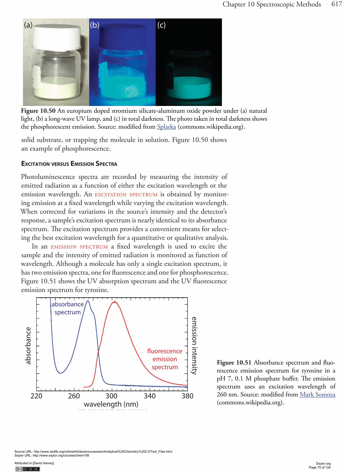
617Chapter 10 Spectroscopic Methods
solid substrate, or trapping the molecule in solution. Figure 10.50 shows an example of phosphorescence.
EXCITATION VERSUS EMISSION SPECTRA
Photoluminescence spectra are recorded by measuring the intensity of emitted radiation as a function of either the excitation wavelength or the emission wavelength. An excitation spectrum is obtained by monitor-ing emission at a fixed wavelength while varying the excitation wavelength. When corrected for variations in the source’s intensity and the detector’s response, a sample’s excitation spectrum is nearly identical to its absorbance spectrum. The excitation spectrum provides a convenient means for select-ing the best excitation wavelength for a quantitative or qualitative analysis.
In an emission spectrum a fixed wavelength is used to excite the sample and the intensity of emitted radiation is monitored as function of wavelength. Although a molecule has only a single excitation spectrum, it has two emission spectra, one for fluorescence and one for phosphorescence. Figure 10.51 shows the UV absorption spectrum and the UV fluorescence emission spectrum for tyrosine.
Figure 10.50 An europium doped strontium silicate-aluminum oxide powder under (a) natural light, (b) a long-wave UV lamp, and (c) in total darkness. The photo taken in total darkness shows the phosphorescent emission. Source: modified from Splarka (commons.wikipedia.org).
Figure 10.51 Absorbance spectrum and fluo-rescence emission spectrum for tyrosine in a pH 7, 0.1 M phosphate buffer. The emission spectrum uses an excitation wavelength of 260 nm. Source: modified from Mark Somoza (commons.wikipedia.org).
(a) (b) (c)
220 380260 300 340wavelength (nm)
abso
rban
ce
absorbancespectrum
fluorescenceemissionspectrum
emission intensity
Source URL: http://www.asdlib.org/onlineArticles/ecourseware/Analytical%20Chemistry%202.0/Text_Files.html Saylor URL: http://www.saylor.org/courses/chem108 Attributed to [David Harvey]
Saylor.org Page 75 of 124

618 Analytical Chemistry 2.0
10F.2 Instrumentation
The basic instrumental needs for monitoring fluorescence and phospho-rescence—a source of radiation, a means of selecting a narrow band of radiation, and a detector—are the same as those for absorption spectros-copy. The unique demands of both techniques, however, require some modifications to the instrument designs seen earlier in Figure 10.25 (filter photometer), Figure 10.26 (single-beam spectrophotometer), Figure 10.27 (double-beam spectrophotometer), and Figure 10.28 (diode array spec-trometer). The most important difference is the detector cannot be placed directly across from the source. Figure 10.52 shows why this is the case. If we place the detector along the source’s axis it will receive both the trans-mitted source radiation, PT, and the fluorescent, If, or phosphorescent, Ip, radiation. Instead, we rotate the director and place it at 90o to the source.
INSTRUMENTS FOR MEASURING FLUORESCENCE
Figure 10.53 shows the basic design of an instrument for measuring fluo-rescence, which includes two wavelength selectors, one for selecting an excitation wavelength from the source and one for selecting the emission wavelength from the sample. In a fluorimeter the excitation and emis-sion wavelengths are selected using absorption or interference filters. The excitation source for a fluorimeter is usually a low-pressure Hg vapor lamp that provides intense emission lines distributed throughout the ultravio-let and visible region (254, 312, 365, 405, 436, 546, 577, 691, and 773 nm). When a monochromator is used to select the excitation and emis-sion wavelengths, the instrument is called a spectrofluorimeter. With a monochromator the excitation source is usually high-pressure Xe arc lamp, which has a continuous emission spectrum. Either instrumental design is
Figure 10.52 Schematic diagram showing the orientation of the source and the detec-tor when measuring fluorescence and phos-phorescence. Contrast this to Figure 10.21, which shows the orientation for absorption spectroscopy.
P0
If or Ip
PT
z-axis
x-axis
y-axis
Source URL: http://www.asdlib.org/onlineArticles/ecourseware/Analytical%20Chemistry%202.0/Text_Files.html Saylor URL: http://www.saylor.org/courses/chem108 Attributed to [David Harvey]
Saylor.org Page 76 of 124

619Chapter 10 Spectroscopic Methods
appropriate for quantitative work, although only a spectrofluorimeter can be used to record an excitation or emission spectrum.
The sample cells for molecular fluorescence are similar to those for molecular absorption. Remote sensing with fiber optic probes also can be adapted for use with either a fluorimeter or spectrofluorimeter. An analyte that is fluorescent can be monitored directly. For analytes that are not fluo-rescent, a suitable fluorescent probe molecule can be incorporated into the tip of the fiber optic probe. The analyte’s reaction with the probe molecule leads to an increase or decrease in fluorescence.
INSTRUMENTS FOR MEASURING PHOSPHORESCENCE
Instrumentation for molecular phosphorescence must discriminate between phosphorescence and fluorescence. Because the lifetime for fluorescence is shorter than that for phosphorescence, discrimination is easily achieved by incorporating a delay between exciting the sample and measuring phos-phorescent emission. Figure 10.54 shows how two out-of-phase choppers can be use to block emission from reaching the detector when the sample is being excited, and to prevent source radiation from reaching the sample while we are measuring the phosphorescent emission.
Because phosphorescence is such a slow process, we must prevent the excited state from relaxing by external conversion. Traditionally, this has been accomplished by dissolving the sample in a suitable organic solvent, usually a mixture of ethanol, isopentane, and diethylether. The resulting solution is frozen at liquid-N2 temperatures, forming an optically clear solid. The solid matrix minimizes external conversion due to collisions be-tween the analyte and the solvent. External conversion also is minimized
Figure 10.53 Schematic diagram for measuring fluores-cence showing the placement of the wavelength selectors for excitation and emission. When a filter is used the instru-ment is called a fluorimeter, and when a monochromator is used the instrument is called a spectrofluorimeter.
Figure 10.54 Schematic diagram showing how choppers are used to prevent fluores-cent emission from interfering with the measurement of phosphorescent emission.
λ1 λ2λ3
λ1 λ2λ3
or
or
source
excitation wavelength selector
monochromator filter
monochrom
atorfilter
emission w
avelength selector
detectorsignal processor
fromsource
todetector
fromsource
todetector
openblocked
Excitating Sample Measuring Emission
choppers
open
openblocked
blocked
Source URL: http://www.asdlib.org/onlineArticles/ecourseware/Analytical%20Chemistry%202.0/Text_Files.html Saylor URL: http://www.saylor.org/courses/chem108 Attributed to [David Harvey]
Saylor.org Page 77 of 124

620 Analytical Chemistry 2.0
by immobilizing the sample on a solid substrate, making possible room temperature measurements. One approach is to place a drop of the solu-tion containing the analyte on a small disc of filter paper. After drying the sample under a heat lamp, the sample is placed in the spectrofluorimeter for analysis. Other solid surfaces that have been used include silica gel, alumina, sodium acetate, and sucrose. This approach is particularly useful for the analysis of thin layer chromatography plates.
10F.3 Quantitative Applications
Molecular fluorescence and, to a lesser extent, phosphorescence have been used for the direct or indirect quantitative analysis of analytes in a variety of matrices. A direct quantitative analysis is possible when the analyte’s fluo-rescent or phosphorescent quantum yield is favorable. When the analyte is not fluorescent or phosphorescent, or if the quantum yield is unfavorable, then an indirect analysis may be feasible. One approach is to react the analyte with a reagent to form a product with fluorescent or phosphores-cent properties. Another approach is to measure a decrease in fluorescence or phosphorescence when the analyte is added to a solution containing a fluorescent or phosphorescent probe molecule. A decrease in emission is observed when the reaction between the analyte and the probe molecule en-hances radiationless deactivation, or produces a nonemittng product. The application of fluorescence and phosphorescence to inorganic and organic analytes are considered in this section.
INORGANIC ANALYTES
Except for a few metal ions, most notably UO2+, most inorganic ions are
not sufficiently fluorescent for a direct analysis. Many metal ions may be de-termined indirectly by reacting with an organic ligand to form a fluorescent, or less commonly, a phosphorescent metal–ligand complex. One example is the reaction of Al3+ with the sodium salt of 2, 4, 3′-trihydroxyazobenzene-5′-sulfonic acid—also known as alizarin garnet R—which forms a fluo-rescent metal–ligand complex (Figure 10.55). The analysis is carried out using an excitation wavelength of 470 nm, monitoring fluorescence at 500 nm. Table 10.12 provides additional examples of chelating reagents that form fluorescent metal–ligand complexes with metal ions. A few inorganic nonmetals are determined by their ability to decrease, or quench, the fluo-rescence of another species. One example is the analysis for F– based on its ability to quench the fluorescence of the Al3+–alizarin garnet R complex.
ORGANIC ANALYTES
As noted earlier, organic compounds containing aromatic rings generally are fluorescent and aromatic heterocycles are often phosphorescent. As shown in Table 10.13, several important biochemical, pharmaceutical, and envi-ronmental compounds may be analyzed quantitatively by fluorimetry or
Figure 10.55 Structure of alizarin gar-net R and its metal–ligand complex with Al3+.
N N
HOOH
OHHO
N
N OH
HO
O
O
Al3+
alizarin garnet R
fluorescent complex
Source URL: http://www.asdlib.org/onlineArticles/ecourseware/Analytical%20Chemistry%202.0/Text_Files.html Saylor URL: http://www.saylor.org/courses/chem108 Attributed to [David Harvey]
Saylor.org Page 78 of 124

621Chapter 10 Spectroscopic Methods
phosphorimetry. If an organic analyte is not naturally fluorescent or phos-phorescent, it may be possible to incorporate it into a chemical reaction that produces a fluorescent or phosphorescent product. For example, the enzyme creatine phosphokinase can be determined by using it to catalyze the formation of creatine from phosphocreatine. Reacting the creatine with ninhydrin produces a fluorescent product of unknown structure.
Table 10.12 Chelating Agents for the Fluorescence Analysis of Metal Ionschelating agent metal ions8-hydroxyquinoline Al3+, Be2+, Zn2+, Li+, Mg2+ (and others)flavonal Zr2+, Sn4+
benzoin B4O72–, Zn2+
2′, 3, 4′, 5, 7-pentahydroxyflavone Be2+
2-(o-hydroxyphenyl) benzoxazole Cd2+
Table 10.13 Examples of Naturally Photoluminescent Organic Analytesclass compounds (F = fluorescence; P = phosphorescence)aromatic amino acids phenylalanine (F)
tyrosine (F)tryptophan (F, P)
vitamins vitamin A (F)vitamin B2 (F)vitamin B6 (F)vitamin B12 (F)vitamin E (F)folic acid (F)
catecholamines dopamine (F)norepinephrine (F)
pharmaceuticals and drugs quinine (F)salicylic acid (F, P)morphine (F)barbiturates (F)LSD (F)codeine (P)caffeine (P)sulfanilamide (P)
environmental pollutants pyrene (F)benzo[a]pyrene (F)organothiophosphorous pesticides (F)carbamate insecticides (F)DDT (P)
Source URL: http://www.asdlib.org/onlineArticles/ecourseware/Analytical%20Chemistry%202.0/Text_Files.html Saylor URL: http://www.saylor.org/courses/chem108 Attributed to [David Harvey]
Saylor.org Page 79 of 124

622 Analytical Chemistry 2.0
STANDARDIZING THE METHOD
From equation 10.28 and equation 10.29 we know that the intensity of fluorescent or phosphorescent emission is a linear function of the analyte’s concentration provided that the sample’s absorbance of source radiation (A = εbC) is less than approximately 0.01. Calibration curves often are linear over four to six orders of magnitude for fluorescence and over two to four orders of magnitude for phosphorescence. For higher concentrations of analyte the calibration curve becomes nonlinear because the assumptions leading to equation 10.28 and equation 10.29 no longer apply. Nonlinear-ity may be observed for small concentrations of analyte due to the presence of fluorescent or phosphorescent contaminants. As discussed earlier, quan-tum efficiency is sensitive to temperature and sample matrix, both of which must be controlled when using external standards. In addition, emission intensity depends on the molar absorptivity of the photoluminescent spe-cies, which is sensitive to the sample matrix.
Representative Method 10.3Determination of Quinine in Urine
DESCRIPTION OF METHOD
Quinine is an alkaloid used in treating malaria. It is a strongly fluorescent compound in dilute solutions of H2SO4 (Φf = 0.55). Quinine’s excitation spectrum has absorption bands at 250 nm and 350 nm and its emission spectrum has a single emission band at 450 nm. Quinine is rapidly ex-creted from the body in urine and is easily determined by measuring its fluorescence following its extraction from the urine sample.
PROCEDURE
Transfer a 2.00-mL sample of urine to a 15-mL test tube and adjust its pH to between 9 and 10 using 3.7 M NaOH. Add 4 mL of a 3:1 (v/v) mixture of chloroform and isopropanol and shake the contents of the test tube for one minute. Allow the organic and the aqueous (urine) layers to separate and transfer the organic phase to a clean test tube. Add 2.00 mL of 0.05 M H2SO4 to the organic phase and shake the contents for one minute. Allow the organic and the aqueous layers to separate and transfer the aque-ous phase to the sample cell. Measure the fluorescent emission at 450 nm using an excitation wavelength of 350 nm. Determine the concentration of quinine in the urine sample using a calibration curve prepared with a set of external standards in 0.05 M H2SO4, prepared from a 100.0 ppm solution of quinine in 0.05 M H2SO4. Use distilled water as a blank.
QUESTIONS
1. Chloride ion quenches the intensity of quinine’s fluorescent emission. For example, in the presence of 100 ppm NaCl (61 ppm Cl–) qui-nine’s emission intensity is only 83% of its emission intensity in the
The best way to appreciate the theoretical and practical details discussed in this sec-tion is to carefully examine a typical ana-lytical method. Although each method is unique, the following description of the determination of quinine in urine pro-vides an instructive example of a typical procedure. The description here is based on Mule, S. J.; Hushin, P. L. Anal. Chem. 1971, 43, 708–711, and O’Reilly, J. E.; J. Chem. Educ. 1975, 52, 610–612.
Figure 10.49 shows the fluorescence of the quinine in tonic water.
Source URL: http://www.asdlib.org/onlineArticles/ecourseware/Analytical%20Chemistry%202.0/Text_Files.html Saylor URL: http://www.saylor.org/courses/chem108 Attributed to [David Harvey]
Saylor.org Page 80 of 124

623Chapter 10 Spectroscopic Methods
Example 10.11
To evaluate the method described in Representative Method 10.3, a se-ries of external standard was prepared and analyzed, providing the results shown in the following table. All fluorescent intensities were corrected using a blank prepared from a quinine-free sample of urine. The fluores-cent intensities are normalized by setting If for the highest concentration standard to 100.
absence of chloride. The presence of 1000 ppm NaCl (610 ppm Cl–) further reduces quinine’s fluorescent emission to less than 30% of its emission intensity in the absence of chloride. The concentration of chloride in urine typically ranges from 4600–6700 ppm Cl–. Explain how this procedure prevents an interference from chloride.
The procedure uses two extractions. In the first of these extractions, quinine is separated from urine by extracting it into a mixture of chlo-roform and isopropanol, leaving the chloride behind in the original sample.
2. Samples of urine may contain small amounts of other fluorescent compounds, which interfere with the analysis if they are carried through the two extractions. Explain how you can modify the proce-dure to take this into account?
One approach is to prepare a blank using a sample of urine known to be free of quinine. Subtracting the blank’s fluorescent signal from the measured fluorescence from urine samples corrects for the interfering compounds.
3. The fluorescent emission for quinine at 450 nm can be induced using an excitation frequency of either 250 nm or 350 nm. The fluorescent quantum efficiency is the same for either excitation wavelength. Qui-nine’s absorption spectrum shows that ε250 is greater than ε350. Given that quinine has a stronger absorbance at 250 nm, explain why its fluorescent emission intensity is greater when using 350 nm as the excitation wavelength.
From equation 10.28 we know that If is a function of the following terms: k, Φf, P0, ε, b, and C. We know that Φf, b, and C are the same for both excitation wavelengths and that ε is larger for a wavelength of 250 nm; we can, therefore, ignore these terms. The greater emis-sion intensity when using an excitation wavelength of 350 nm must be due to a larger value for P0 or k . In fact, P0 at 350 nm for a high-pressure Xe arc lamp is about 170% of that at 250 nm. In addition, the sensitivity of a typical photomultiplier detector (which contrib-utes to the value of k) at 350 nm is about 140% of that at 250 nm.
Source URL: http://www.asdlib.org/onlineArticles/ecourseware/Analytical%20Chemistry%202.0/Text_Files.html Saylor URL: http://www.saylor.org/courses/chem108 Attributed to [David Harvey]
Saylor.org Page 81 of 124

624 Analytical Chemistry 2.0
[quinine] (μg/mL) If1.00 10.113.00 30.205.00 49.847.00 69.89
10.00 100.0
After ingesting 10.0 mg of quinine, a volunteer provided a urine sample 24-h later. Analysis of the urine sample gives an relative emission intensity of 28.16. Report the concentration of quinine in the sample in mg/L and the percent recovery for the ingested quinine.
SOLUTION
Linear regression of the relative emission intensity versus the concentration of quinine in the standards gives a calibration curve with the following equation.
I f
g quininemL
= + ×0 124 9 978. .
Substituting the sample’s relative emission intensity into the calibration equation gives the concentration of quinine as 2.81 μg/mL. Because the volume of urine taken, 2.00 mL, is the same as the volume of 0.05 M H2SO4 used in extracting quinine, the concentration of quinine in the urine also is 2.81 μg/mL. The recovery of the ingested quinine is
2 81 2 00 1
10
. .gml urine
mL urine mg1000 g
× ×
... %
0100 0 0562
mg quinine ingested× =
10F.4 Evaluation of Photoluminescence Spectroscopy
SCALE OF OPERATION
Photoluminescence spectroscopy is used for the routine analysis of trace and ultratrace analytes in macro and meso samples. Detection limits for fluorescence spectroscopy are strongly influenced by the analyte’s quantum yield. For an analyte with Φf > 0.5, a picomolar detection limit is possible when using a high quality spectrofluorimeter. For example, the detection limit for quinine sulfate, for which Φf is 0.55, is generally between 1 part per billion and 1 part per trillion. Detection limits for phosphorescence are somewhat higher, with typical values in the nanomolar range for low-temperature phosphorimetry, and in the micromolar range for room-tem-perature phosphorimetry using a solid substrate.
It can take up 10–11 days for the body to completely excrete quinine.
See Figure 3.5 to review the meaning of macro and meso for describing samples, and the meaning of major, minor, and ul-tratrace for describing analytes.
0 2 4 6 8 10
0
20
40
60
80
100
rela
tive
emis
sion
inte
nsity
μg quinine/mL
Source URL: http://www.asdlib.org/onlineArticles/ecourseware/Analytical%20Chemistry%202.0/Text_Files.html Saylor URL: http://www.saylor.org/courses/chem108 Attributed to [David Harvey]
Saylor.org Page 82 of 124

625Chapter 10 Spectroscopic Methods
ACCURACY
The accuracy of a fluorescence method is generally between 1–5% when spectral and chemical interferences are insignificant. Accuracy is limited by the same types of problems affecting other optical spectroscopic methods. In addition, accuracy is affected by interferences influencing the fluorescent quantum yield. The accuracy of phosphorescence is somewhat greater than that for fluorescence.
PRECISION
The relative standard deviation for fluorescence is usually between 0.5–2% when the analyte’s concentration is well above its detection limit. Precision is usually limited by the stability of the excitation source. The precision for phosphorescence is often limited by reproducibility in preparing samples for analysis, with relative standard deviations of 5–10% being common.
SENSITIVITY
From equation 10.28 and equation 10.29 we know that the sensitivity of a fluorescent or phosphorescent method is influenced by a number of pa-rameters. The importance of quantum yield and the effect of temperature and solution composition on Φf and Φp already have been considered. Besides quantum yield, the sensitivity of an analysis can be improved by using an excitation source that has a greater emission intensity, P0, at the desired wavelength, and by selecting an excitation wavelength that has a greater absorbance. Another approach for improving sensitivity is to in-crease the volume in the sample from which emission is monitored. Figure 10.56 shows how rotating a monochromator’s slits from their usual vertical orientation to a horizontal orientation increases the sampling volume. The result can increase the emission from the sample by 5–30×.
Figure 10.56 Use of slit orientation to change the volume from which fluorescence is measured: (a) vertical slit orientation; (b) horizontal slit orientation. Suppose the slit’s dimensions are 0.1 mm × 3 mm. In (a) the dimensions of the sampling volume are 0.1 mm × 0.1mm × 3 mm, or 0.03 mm3. For (b) the dimensions of the sampling volume are 0.1 mm × 3 mm × 3 mm, or 0.9 mm3, a 30-fold increase in the sampling volume.
(a) (b)
fromsource
fromsource
todetector
todetector
Source URL: http://www.asdlib.org/onlineArticles/ecourseware/Analytical%20Chemistry%202.0/Text_Files.html Saylor URL: http://www.saylor.org/courses/chem108 Attributed to [David Harvey]
Saylor.org Page 83 of 124

626 Analytical Chemistry 2.0
SELECTIVITY
The selectivity of fluorescence and phosphorescence is superior to that of absorption spectrophotometry for two reasons: first, not every compound that absorbs radiation is fluorescent or phosphorescent; and, second, selec-tivity between an analyte and an interferent is possible if there is a difference in either their excitation or their emission spectra. The total emission in-tensity is a linear sum of that from each fluorescent or phosphorescent spe-cies. The analysis of a sample containing n components, therefore, can be accomplished by measuring the total emission intensity at n wavelengths.
TIME, COST, AND EQUIPMENT
As with other optical spectroscopic methods, fluorescent and phosphores-cent methods provide a rapid means for analyzing samples and are capable of automation. Fluorimeters are relatively inexpensive, ranging from several hundred to several thousand dollars, and often are satisfactory for quan-titative work. Spectrofluorimeters are more expensive, with models often exceeding $50,000.
10G Atomic Emission Spectroscopy
The focus of this section is on the emission of ultraviolet and visible ra-diation following the thermal excitation of atoms. Atomic emission spec-troscopy has a long history. Qualitative applications based on the color of flames were used in the smelting of ores as early as 1550 and were more fully developed around 1830 with the observation of atomic spectra generated by flame emission and spark emission.18 Quantitative applications based on the atomic emission from electric sparks were developed by Lockyer in the early 1870 and quantitative applications based on flame emission were pioneered by Lundegardh in 1930. Atomic emission based on emission from a plasma was introduced in 1964.
10G.1 Atomic Emission Spectra
Atomic emission occurs when a valence electron in a higher energy atomic orbital returns to a lower energy atomic orbital. Figure 10.57 shows a por-tion of the energy level diagram for sodium, which consists of a series of discrete lines at wavelengths corresponding to the difference in energy be-tween two atomic orbitals.
The intensity of an atomic emission line, Ie, is proportional to the num-ber of atoms, N*, populating the excited state,
I kNe *= 10.30
where k is a constant accounting for the efficiency of the transition. If a system of atoms is in thermal equilibrium, the population of excited state i is related to the total concentration of atoms, N, by the Boltzmann distribu-18 Dawson, J. B. J. Anal. At. Spectrosc. 1991, 6, 93–98.
Figure 10.57 Valence shell energy level diagram for sodium. The wavelengths corresponding to several transitions are shown. Note that this is the same en-ergy level diagram as Figure 10.19.
1138.3
589.6 589.0
819.5
818.3330.2
330.3
1140.4
3s
3p
3d
4s
4p
4d
5s
5p
Ener
gy
Source URL: http://www.asdlib.org/onlineArticles/ecourseware/Analytical%20Chemistry%202.0/Text_Files.html Saylor URL: http://www.saylor.org/courses/chem108 Attributed to [David Harvey]
Saylor.org Page 84 of 124

627Chapter 10 Spectroscopic Methods
tion. For many elements at temperatures of less than 5000 K the Boltzmann distribution is approximated as
N Ngg
e* /i E kT
0
i 10.31
where gi and g0 are statistical factors that account for the number of equiva-lent energy levels for the excited state and the ground state, Ei is the energy of the excited state relative to a ground state energy, E0, of 0, k is Boltz-mann’s constant (1.3807 × 10⁻²³ J/K), and T is the temperature in kelvin. From equation 10.31 we expect that excited states with lower energies have larger populations and more intense emission lines. We also expect emis-sion intensity to increase with temperature.
10G.2 Equipment
An atomic emission spectrometer is similar in design to the instrumenta-tion for atomic absorption. In fact, it is easy to adapt most flame atomic absorption spectrometers for atomic emission by turning off the hollow cathode lamp and monitoring the difference in the emission intensity when aspirating the sample and when aspirating a blank. Many atomic emission spectrometers, however, are dedicated instruments designed to take advan-tage of features unique to atomic emission, including the use of plasmas, arcs, sparks, and lasers as atomization and excitation sources, and an en-hanced capability for multielemental analysis.
ATOMIZATION AND EXCITATION
Atomic emission requires a means for converting a solid, liquid, or solution analyte into a free gaseous atom. The same source of thermal energy usu-ally serves as the excitation source. The most common methods are flames and plasmas, both of which are useful for liquid or solution samples. Solid samples may be analyzed by dissolving in a solvent and using a flame or plasma atomizer.
FLAME SOURCES
Atomization and excitation in flame atomic emission is accomplished using the same nebulization and spray chamber assembly used in atomic absorp-tion (Figure 10.42). The burner head consists of single or multiple slots, or a Meker style burner. Older atomic emission instruments often used a total consumption burner in which the sample is drawn through a capillary tube and injected directly into the flame.
PLASMA SOURCES
A plasma is a hot, partially ionized gas that contains an abundant concen-tration of cations and electrons. The plasmas used in atomic emission are formed by ionizing a flowing stream of argon gas, producing argon ions and
Source URL: http://www.asdlib.org/onlineArticles/ecourseware/Analytical%20Chemistry%202.0/Text_Files.html Saylor URL: http://www.saylor.org/courses/chem108 Attributed to [David Harvey]
Saylor.org Page 85 of 124

628 Analytical Chemistry 2.0
electrons. A plasma’s high temperature results from resistive heating as the electrons and argon ions move through the gas. Because plasmas operate at much higher temperatures than flames, they provide better atomization and a higher population of excited states.
A schematic diagram of the inductively coupled plasma source (ICP) is shown in Figure 10.58. The ICP torch consists of three concentric quartz tubes, surrounded at the top by a radio-frequency induction coil. The sample is mixed with a stream of Ar using a nebulizer, and is carried to the plasma through the torch’s central capillary tube. Plasma formation is initiated by a spark from a Tesla coil. An alternating radio-frequency cur-rent in the induction coils creates a fluctuating magnetic field that induces the argon ions and the electrons to move in a circular path. The resulting collisions with the abundant unionized gas give rise to resistive heating, providing temperatures as high as 10 000 K at the base of the plasma, and between 6000 and 8000 K at a height of 15–20 mm above the coil, where emission is usually measured. At these high temperatures the outer quartz tube must be thermally isolated from the plasma. This is accomplished by the tangential flow of argon shown in the schematic diagram.
MULTIELEMENTAL ANALYSIS
Atomic emission spectroscopy is ideally suited for multielemental analysis because all analytes in a sample are excited simultaneously. If the instrument includes a scanning monochromator, we can program it to move rapidly to an analyte’s desired wavelength, pause to record its emission intensity, and then move to the next analyte’s wavelength. This sequential analysis allows for a sampling rate of 3–4 analytes per minute.
Another approach to a multielemental analysis is to use a multichan-nel instrument that allows us to simultaneously monitor many analytes. A simple design for a multichannel spectrometer couples a monochroma-tor with multiple detectors that can be positioned in a semicircular array around the monochromator at positions corresponding to the wavelengths for the analytes (Figure 10.59).
10G.3 Quantitative Applications
Atomic emission is widely used for the analysis of trace metals in a variety of sample matrices. The development of a quantitative atomic emission method requires several considerations, including choosing a source for atomization and excitation, selecting a wavelength and slit width, prepar-ing the sample for analysis, minimizing spectral and chemical interferences, and selecting a method of standardization.
CHOICE OF ATOMIZATION AND EXCITATION SOURCE
Except for the alkali metals, detection limits when using an ICP are sig-nificantly better than those obtained with flame emission (Table 10.14).
Figure 10.58 Schematic diagram of an inductively coupled plasma torch. Source: modified from Xvlun (commons.wikipe-dia.org).
quartz bonnet
RF induction coil
capillary injection tube
tangential Ar flow
Ar plasma gas inlet
sample aerosol inlet
plasma tube
coolent tube
6000 K
8000 K
10 000 K
Source URL: http://www.asdlib.org/onlineArticles/ecourseware/Analytical%20Chemistry%202.0/Text_Files.html Saylor URL: http://www.saylor.org/courses/chem108 Attributed to [David Harvey]
Saylor.org Page 86 of 124

629Chapter 10 Spectroscopic Methods
Figure 10.59 Schematic diagram of a multichannel atom-ic emission spectrometer for the simultaneous analysis of several elements. The ICP torch is modified from Xvlun (commons.wikipedia.org). Instruments may contain as many as 48–60 detectors.
Table 10.14 Detection Limits for Atomic Emissiona
detection limit in μg/mLelement flame emission ICP
Ag 2 0.2Al 3 0.2As 2000 2Ca 0.1 0.0001Cd 300 0.07Co 5 0.1Cr 1 0.08Fe 10 0.09Hg 150 1K 0.01 30Li 0.001 0.02Mg 1 0.003Mn 1 0.01Na 0.01 0.1Ni 10 0.2Pb 0.2 1Pt 2000 0.9Sn 100 3Zn 1000 0.1
a Source: Parsons, M. L.; Major, S.; Forster, A. R.; App. Spectrosc. 1983, 37, 411–418.
λ1 λ2λ3
ICP torchmonochromator
detector 1
detector 2
detector 3 detector 4
detector 5
detector 6
Source URL: http://www.asdlib.org/onlineArticles/ecourseware/Analytical%20Chemistry%202.0/Text_Files.html Saylor URL: http://www.saylor.org/courses/chem108 Attributed to [David Harvey]
Saylor.org Page 87 of 124

630 Analytical Chemistry 2.0
Plasmas also are subject to fewer spectral and chemical interferences. For these reasons a plasma emission source is usually the better choice.
SELECTING THE WAVELENGTH AND SLIT WIDTH
The choice of wavelength is dictated by the need for sensitivity and the need to avoid interferences from the emission lines of other constituents in the sample. Because an analyte’s atomic emission spectrum has an abundance of emission lines—particularly when using a high temperature plasma source—it is inevitable that there will be some overlap between emission lines. For example, an analysis for Ni using the atomic emission line at 349.30 nm is complicated by the atomic emission line for Fe at 349.06 nm. Narrower slit widths provide better resolution, but at the cost of less radia-tion reaching the detector. The easiest approach to selecting a wavelength is to record the sample’s emission spectrum and look for an emission line that provides an intense signal and is resolved from other emission lines.
PREPARING THE SAMPLE
Flame and plasma sources are best suited for samples in solution and liquid form. Although a solid sample can be analyzed by directly inserting it into the flame or plasma, they usually are first brought into solution by diges-tion or extraction.
MINIMIZING SPECTRAL INTERFERENCES
The most important spectral interference is broad, background emission from the flame or plasma and emission bands from molecular species. This background emission is particularly severe for flames because the tempera-ture is insufficient to break down refractory compounds, such as oxides and hydroxides. Background corrections for flame emission are made by scanning over the emission line and drawing a baseline (Figure 10.60). Because a plasma’s temperature is much higher, a background interference due to molecular emission is less of a problem. Although emission from the plasma’s core is strong, it is insignificant at a height of 10–30 mm above the core where measurements normally are made.
MINIMIZING CHEMICAL INTERFERENCES
Flame emission is subject to the same types of chemical interferences as atomic absorption. These interferences are minimized by adjusting the flame’s composition and adding protecting agents, releasing agents, or ion-ization suppressors. An additional chemical interference results from self-absorption. Because the flame’s temperature is greatest at its center, the concentration of analyte atoms in an excited state is greater at the flame’s center than at its outer edges. If an excited state atom in the flame’s center emits a photon while returning to its ground state, then a ground state atom in the cooler, outer regions of the flame may absorb the photon, decreasing
Figure 10.60 Method for correcting an analyte’s emission for the flame’s background emission.
emis
sion
inte
nsity
Ie
wavelength
Source URL: http://www.asdlib.org/onlineArticles/ecourseware/Analytical%20Chemistry%202.0/Text_Files.html Saylor URL: http://www.saylor.org/courses/chem108 Attributed to [David Harvey]
Saylor.org Page 88 of 124

631Chapter 10 Spectroscopic Methods
the emission intensity. For higher concentrations of analyte self-absorption may invert the center of the emission band (Figure 10.61).
Chemical interferences with plasma sources generally are not significant because the plasma’s higher temperature limits the formation of nonvola-tile species. For example, PO4
3– is a significant interferent when analyzing samples for Ca2+ by flame emission, but has a negligible effect when using a plasma source. In addition, the high concentration of electrons from the ionization of argon minimizes ionization interferences.
STANDARDIZING THE METHOD
From equation 10.30 we know that emission intensity is proportional to the population of the analyte’s excited state, N*. If the flame or plasma is in thermal equilibrium, then the excited state population is proportional to the analyte’s total population, N, through the Boltzmann distribution (equation 10.31).
A calibration curve for flame emission is usually linear over two to three orders of magnitude, with ionization limiting linearity when the analyte’s concentrations is small and self-absorption limiting linearity for higher concentrations of analyte. When using a plasma, which suffers from fewer chemical interferences, the calibration curve often is linear over four to five orders of magnitude and is not affected significantly by changes in the matrix of the standards.
Emission intensity may be affected significantly by many parameters, including the temperature of the excitation source and the efficiency of atomization. An increase in temperature of 10 K, for example, produces a 4% increase in the fraction of Na atoms occupying the 3p excited state. This is potentially significant uncertainty that may limit the use of external standards. The method of internal standards can be used when variations in source parameters are difficult to control. To compensate for changes in the temperature of the excitation source, the internal standard is selected so that its emission line is close to the analyte’s emission line. In addition, the internal standard should be subject to the same chemical interferences to compensate for changes in atomization efficiency. To accurately compen-sate for these errors the analyte and internal standard emission lines must be monitored simultaneously.
Figure 10.61 Atomic emission lines for (a) a low concentration of analyte, and (b) a high concentration of analyte showing the effect of self-absorption.
Representative Method 10.4Determination of Sodium in a Salt Substitute
DESCRIPTION OF METHOD
Salt substitutes, which are used in place of table salt for individuals on low–sodium diets, replaces NaCl with KCl. Depending on the brand, fumaric acid, calcium hydrogen phosphate, or potassium tartrate also may be present. Although intended to be sodium-free, salt substitutes contain small amounts of NaCl as an impurity. Typically, the concentration of
The best way to appreciate the theoretical and practical details discussed in this sec-tion is to carefully examine a typical ana-lytical method. Although each method is unique, the following description of the determination of sodium in salt substi-tutes provides an instructive example of a typical procedure. The description here is based on Goodney, D. E. J. Chem. Educ. 1982, 59, 875–876.
(a) (b)
Source URL: http://www.asdlib.org/onlineArticles/ecourseware/Analytical%20Chemistry%202.0/Text_Files.html Saylor URL: http://www.saylor.org/courses/chem108 Attributed to [David Harvey]
Saylor.org Page 89 of 124

632 Analytical Chemistry 2.0
sodium in a salt substitute is about 100 μg/g The exact concentration of sodium is easily determined by flame atomic emission. Because it is difficult to match the matrix of the standards to that of the sample, the analysis is accomplished by the method of standard additions.
PROCEDURE
A sample is prepared by placing an approximately 10-g portion of the salt substitute in 10 mL of 3 M HCl and 100 mL of distilled water. After the sample has dissolved, it is transferred to a 250-mL volumetric flask and diluted to volume with distilled water. A series of standard additions is prepared by placing 25-mL portions of the diluted sample into separate 50-mL volumetric flasks, spiking each with a known amount of an ap-proximately 10 mg/L standard solution of Na+, and diluting to volume. After zeroing the instrument with an appropriate blank, the instrument is optimized at a wavelength of 589.0 nm while aspirating a standard solu-tion of Na+. The emission intensity is measured for each of the standard addition samples and the concentration of sodium in the salt substitute is reported in μg/g.
QUESTIONS
1. Potassium ionizes more easily than sodium. What problem might this present if you use external standards prepared from a stock solution of 10 mg Na/L instead of using a set of standard additions?
Because potassium is present at a much higher concentration than sodium, its ionization suppresses the ionization of sodium. Normally suppressing ionization is a good thing because it increases emission intensity. In this case, however, the difference between the matrix of the standards and the sample’s matrix means that the sodium in a standard experiences more ionization than an equivalent amount of sodium in a sample. The result is a determinate error.
2. One way to avoid a determinate error when using external standards is to match the matrix of the standards to that of the sample. We could, for example, prepare external standards using reagent grade KCl to match the matrix to that of the sample. Why is this not a good idea for this analysis?
Sodium is a common contaminant, which is found in many chemi-cals. Reagent grade KCl, for example, may contain 40–50 μg Na/g. This is a significant source of sodium, given that the salt substitute contains approximately 100 μg Na/g..
3. Suppose you decide to use an external standardization. Given the answer to the previous questions, is the result of your analysis likely to underestimate or overestimate the amount of sodium in the salt substitute?
Source URL: http://www.asdlib.org/onlineArticles/ecourseware/Analytical%20Chemistry%202.0/Text_Files.html Saylor URL: http://www.saylor.org/courses/chem108 Attributed to [David Harvey]
Saylor.org Page 90 of 124

633Chapter 10 Spectroscopic Methods
The solid black line in Figure 10.62 shows the ideal calibration curve assuming that we match the matrix of the standards to the sample’s matrix, and that we do so without adding an additional sodium. If we prepare the external standards without adding KCl, the emission for each standard decreases due to increased ionization. This is shown by the lower of the two dashed red lines. Preparing the standards by adding reagent grade KCl increases the concentration of sodium due to its contamination. Because we underestimate the actual concen-tration of sodium in the standards, the resulting calibration curve is shown by the other dashed red line. In both cases, the sample’s emis-sion results in our overestimating the concentration of sodium in the sample.
4. One problem with analyzing salt samples is their tendency to clog the aspirator and burner assembly. What effect does this have on the analysis?
Clogging the aspirator and burner assembly decreases the rate of aspi-ration, which decreases the analyte’s concentration in the flame. The result is a decrease in the emission intensity and a negative determi-nate error.
Figure 10.62 External standards calibration curves for the flame atomic emission analysis of Na in a salt substitute. The solid black line shows the ideal calibration curve assuming matrix matching of samples and standards with pure KCl. The lower of the two dashed red lines shows the effect of failing to add KCl to the external standards, which decreases emission. The other dashed red line shows the effect of using KCl that is contaminated with NaCl, which causes us to underesti-mate the concentration of Na in the standards. In both cases, the result is a positive determinate error in the analysis of samples.
decrease in emission due to ionization
not accounting forextra sodium
idealcalibration curve
actualconcentration
reportedconcentrations
mg Na/L
emis
sion
sample’semission
Source URL: http://www.asdlib.org/onlineArticles/ecourseware/Analytical%20Chemistry%202.0/Text_Files.html Saylor URL: http://www.saylor.org/courses/chem108 Attributed to [David Harvey]
Saylor.org Page 91 of 124

634 Analytical Chemistry 2.0
Example 10.12
To evaluate the method described in Representative Method 10.4, a series of standard additions is prepared using a 10.0077-g sample of a salt sub-stitute. The results of a flame atomic emission analysis of the standards is shown here.19
added Na (μg/mL) Ie (arb. units)0.000 1.790.420 2.631.051 3.542.102 4.943.153 6.18
What is the concentration of sodium, in μg/g, in the salt substitute.
SOLUTION
Linear regression of emission intensity versus the concentration of added Na gives a standard additions calibration curve with the following equa-tion.
I e
g NamL
= + ×1 97 1 37. .
The concentration of sodium in the sample is equal to the absolute value of the calibration curve’s x-intercept. Substituting zero for the emission in-tensity and solving for sodium’s concentration gives a result of 1.44 μg Na/mL. The concentration of sodium in the salt substitute is
1 44 50 0025 00
250 0. ..
.g NamL
mLmL
mL
10.00
× ×
777 g sampleg Na/g= 71 9.
10G.4 Evaluation of Atomic Emission Spectroscopy
SCALE OF OPERATION
The scale of operations for atomic emission is ideal for the direct analysis of trace and ultratrace analytes in macro and meso samples. With appro-priate dilutions, atomic emission also can be applied to major and minor analytes.
ACCURACY
When spectral and chemical interferences are insignificant, atomic emis-sion is capable of producing quantitative results with accuracies of between 19 Goodney, D. E. J. Chem. Educ. 1982, 59, 875–876
See Section 5C.3 in Chapter 5 to review the method of standard additions.
See Figure 3.5 to review the meaning of macro and meso for describing samples, and the meaning of major, minor, and ul-tratrace for describing analytes.
-2 -1 0 1 2 3 4
0
1
2
3
4
5
6
7
μg Na/mL
emis
sion
inte
nsity
(arb
itrar
y un
its)
Source URL: http://www.asdlib.org/onlineArticles/ecourseware/Analytical%20Chemistry%202.0/Text_Files.html Saylor URL: http://www.saylor.org/courses/chem108 Attributed to [David Harvey]
Saylor.org Page 92 of 124

635Chapter 10 Spectroscopic Methods
1–5%. Accuracy frequently is limited by chemical interferences. Because the higher temperature of a plasma source gives rise to more emission lines, the accuracy of using plasma emission often is limited by stray radiation from overlapping emission lines.
PRECISION
For samples and standards in which the analyte’s concentration exceeds the detection limit by at least a factor of 50, the relative standard deviation for both flame and plasma emission is about 1–5%. Perhaps the most impor-tant factor affecting precision is the stability of the flame’s or the plasma’s temperature. For example, in a 2500 K flame a temperature fluctuation of ±2.5 K gives a relative standard deviation of 1% in emission intensity. Significant improvements in precision may be realized when using internal standards.
SENSITIVITY
Sensitivity is strongly influenced by the temperature of the excitation source and the composition of the sample matrix. Sensitivity is optimized by as-pirating a standard solution of analyte and maximizing the emission by adjusting the flame’s composition and the height from which we monitor the emission. Chemical interferences, when present, decrease the sensitiv-ity of the analysis. The sensitivity of plasma emission is less affected by the sample matrix. In some cases a calibration curve prepared using standards in a matrix of distilled water can be used for samples with more complex matrices.
SELECTIVITY
The selectivity of atomic emission is similar to that of atomic absorption. Atomic emission has the further advantage of rapid sequential or simulta-neous analysis.
TIME, COST, AND EQUIPMENT
Sample throughput with atomic emission is very rapid when using auto-mated systems capable of multielemental analysis. For example, sampling rates of 3000 determinations per hour have been achieved using a multi-channel ICP, and 300 determinations per hour with a sequential ICP. Flame emission is often accomplished using an atomic absorption spectrometer, which typically costs between $10,000–$50,000. Sequential ICP’s range in price from $55,000–$150,000, while an ICP capable of simultaneous multielemental analysis costs between $80,000–$200,000. Combination ICP’s that are capable of both sequential and simultaneous analysis range in price from $150,000–$300,000. The cost of Ar, which is consumed in significant quantities, can not be overlooked when considering the expense of operating an ICP.
Source URL: http://www.asdlib.org/onlineArticles/ecourseware/Analytical%20Chemistry%202.0/Text_Files.html Saylor URL: http://www.saylor.org/courses/chem108 Attributed to [David Harvey]
Saylor.org Page 93 of 124

636 Analytical Chemistry 2.0
10H Spectroscopy Based on Scattering
The blue color of the sky during the day and the red color of the sun at sun-set result from the scattering of light by small particles of dust, molecules of water, and other gases in the atmosphere. The efficiency of a photon’s scattering depends on its wavelength. We see the sky as blue during the day because violet and blue light scatter to a greater extent than other, longer wavelengths of light. For the same reason, the sun appears red at sunset be-cause red light is less efficiently scattered and is more likely to pass through the atmosphere than other wavelengths of light. The scattering of radiation has been studied since the late 1800s, with applications beginning soon thereafter. The earliest quantitative applications of scattering, which date from the early 1900s, used the elastic scattering of light by colloidal suspen-sions to determine the concentration of colloidal particles.
10H.1 Origin of Scattering
If we send a focused, monochromatic beam of radiation with a wavelength λ through a medium of particles with dimensions <1.5λ, the radiation scatters in all directions. For example, visible radiation of 500 nm is scat-tered by particles as large as 750 nm in the longest dimension. Two general categories of scattering are recognized. In elastic scattering, radiation is first absorbed by the particles and then emitted without undergoing change in the radiation’s energy. When the radiation emerges with a change in energy, the scattering is said to be inelastic. Only elastic scattering is considered in this text.
Elastic scattering is divided into two types: Rayleigh, or small-particle scattering, and large-particle scattering. Rayleigh scattering occurs when the scattering particle’s largest dimension is less than 5% of the radiation’s wavelength. The intensity of the scattered radiation is proportional to its frequency to the fourth power, ν4—accounting for the greater scattering of blue light than red light—and is symmetrically distributed (Figure 10.63a). For larger particles, scattering increases in the forward direction and de-creases in the backwards direction as the result of constructive and destruc-tive interferences (Figure 10.63b).
10H.2 Turbidimetry and Nephelometry
Turbidimetry and nephelometry are two techniques based on the elastic scattering of radiation by a suspension of colloidal particles. In turbidi-metry the detector is placed in line with the source and the decrease in the radiation’s transmitted power is measured. In nephelometry scattered radiation is measured at an angle of 90o to the source. The similarity of turbidimetry to absorbance and of nephelometry to fluorescence is evident in the instrumental designs shown in Figure 10.64. In fact, turbidity can be measured using a UV/Vis spectrophotometer and a spectrofluorimeter is suitable for nephelometry.
Figure 10.63 Distribution of radia-tion for (a) Rayleigh, or small-particle scattering, and (b) large-particle scat-tering.
source
source
sample
(a)
(b)
Source URL: http://www.asdlib.org/onlineArticles/ecourseware/Analytical%20Chemistry%202.0/Text_Files.html Saylor URL: http://www.saylor.org/courses/chem108 Attributed to [David Harvey]
Saylor.org Page 94 of 124

637Chapter 10 Spectroscopic Methods
TURBIDIMETRY OR NEPHELOMETRY?
When developing a scattering method the choice of using turbidimetry or nephelometry is determined by two factors. The most important consider-ation is the intensity of the scattered radiation relative to the intensity of the source’s radiation. If the solution contains a small concentration of scatter-ing particles the intensity of the transmitted radiation, IT, is approximately the same as the intensity of the source’s radiation, I0. As we learned earlier in the section on molecular absorption, there is substantial uncertainty in determining a small difference between two intense signals. For this reason, nephelometry is a more appropriate choice for samples containing few scat-tering particles. Turbidimetry is a better choice when the sample contains a high concentration of scattering particles.
A second consideration in choosing between turbidimetry and neph-elometry is the size of the scattering particles. For nephelometry, the inten-sity of scattered radiation at 90o increases when the particles are small and Rayleigh scattering is in effect. For larger particles, as shown in Figure 10.63, the intensity of scattering is diminished at 90o. When using an ultraviolet or visible source of radiation, the optimum particle size is 0.1–1 μm. The size of the scattering particles is less important for turbidimetry where the signal is the relative decrease in transmitted radiation. In fact, turbidimetric measurements are still feasible even when the size of the scattering particles results in an increase in reflection and refraction, although a linear relation-ship between the signal and the concentration of scattering particles may no longer hold.
DETERMINING CONCENTRATION BY TURBIDIMETRY
In turbidimetry the measured transmittance, T, is the ratio of the intensity of source radiation transmitted by the sample, IT, to the intensity of source radiation transmitted by a blank, I0.
Figure 10.64 Schematic diagrams for (a) a turbime-ter, and (b) a nephelometer.
shutter
source
λ1 λ2λ3
open
closedmonochromator
detector
shuttersignal
processor
source
λ1 λ2λ3
open
closedmonochromator
detector
signalprocessor
(a)
(b)
sample or blank
sample or blank
Source URL: http://www.asdlib.org/onlineArticles/ecourseware/Analytical%20Chemistry%202.0/Text_Files.html Saylor URL: http://www.saylor.org/courses/chem108 Attributed to [David Harvey]
Saylor.org Page 95 of 124

638 Analytical Chemistry 2.0
TIIT=0
The relationship between transmittance and the concentration of the scat-tering particles is similar to that given by Beer’s law
− =logT kbC 10.32where C is the concentration of the scattering particles in mass per unit volume (w/v), b is the pathlength, and k is a constant that depends on sev-eral factors, including the size and shape of the scattering particles and the wavelength of the source radiation. As with Beer’s law, equation 10.32 may show appreciable deviations from linearity. The exact relationship is estab-lished by a calibration curve prepared using a series of standards containing known concentrations of analyte.
DETERMINING CONCENTRATION BY NEPHELOMETRY
In nephelometry the relationship between the intensity of scattered radia-tion, IS, and the concentration of scattering particles is
I k I CS S= 0 10.33
where kS is an empirical constant for the system and I0 is the source ra-diation’s intensity. The value of kS is determined from a calibration curve prepared using a series of standards containing known concentrations of analyte.
SELECTING A WAVELENGTH FOR THE INCIDENT RADIATION
The choice of wavelength is based primarily on the need to minimize poten-tial interferences. For turbidimetry, where the incident radiation is transmit-ted through the sample, a monochromator or filter allow us to avoid wave-lengths that are absorbed by the sample. For nephelometry, the absorption of incident radiation is not a problem unless it induces fluorescence from the sample. With a nonfluorescent sample there is no need for wavelength selection, and a source of white light may be used as the incident radia-tion. For both techniques, other considerations in choosing a wavelength including the effect of wavelength on scattering intensity, the transducer’s sensitivity, and the source’s intensity. For example, many common photon transducers are more sensitive to radiation at 400 nm than at 600 nm.
PREPARING THE SAMPLE FOR ANALYSIS
Although equation 10.32 and equation 10.33 relate scattering to the con-centration of scattering particles, the intensity of scattered radiation is also influenced by the particle’s size and shape. Samples containing the same number of scattering particles may show significantly different values for -logT or IS, depending on the average diameter of the particles. For a quan-
Source URL: http://www.asdlib.org/onlineArticles/ecourseware/Analytical%20Chemistry%202.0/Text_Files.html Saylor URL: http://www.saylor.org/courses/chem108 Attributed to [David Harvey]
Saylor.org Page 96 of 124

639Chapter 10 Spectroscopic Methods
titative analysis, therefore, it is necessary to maintain a uniform distribution of particle sizes throughout the sample and between samples and stan-dards.
Most turbidimetric and nephelometric methods rely on precipitation to form the scattering particles. As we learned in Chapter 8, the properties of a precipitate are determined by the conditions under which it forms. To maintain a reproducible distribution of particle sizes between samples and standards, it is necessary to control parameters such as the concentration of reagents, the order of adding reagents, the pH and temperature, the agitation or stirring rate, the ionic strength, and the time between the precipitate’s initial formation and the measurement of transmittance or scattering. In many cases a surface-active agent—such as glycerol, gelatin, or dextrin—is added to stabilize the precipitate in a colloidal state and to prevent the coagulation of the particles.
APPLICATIONS
Turbidimetry and nephelometry are widely used to determine the clarity of water, beverages, and food products. For example, a nephelometric de-termination of the turbidity of water compares the sample’s scattering to the scattering of a set of standards. The primary standard for measuring turbidity is formazin, which is an easily prepared, stable polymer suspen-sion (Figure 10.65).20 Formazin prepared by mixing a 1 g/100 mL solution of hydrazine sulfate, N2H4
.H2SO4, with a 10 g/100 mL solution of hex-amethylenetetramine produces a suspension that is defined as 4000 neph-elometric turbidity units (NTU). A set of standards with NTUs between 0 and 40 is prepared and used to construct a calibration curve. This method is readily adapted to the analysis of the clarity of orange juice, beer, and maple syrup.
A number of inorganic cations and anions can be determined by pre-cipitating them under well-defined conditions and measuring the transmit-tance or scattering of radiation from the precipitated particles. The trans-
20 Hach, C. C.; Bryant, M. “Turbidity Standards,” Technical Information Series, Booklet No. 12, Hach Company: Loveland, CO, 1995.
Figure 10.65 Scheme for preparing for-mazin for use as a turbidity standard.
NN
N
N
+ 6H2O + 2H2SO4 6H2CO + 2(NH4)SO4
nH2CO + (n/2)H2NNH2 + nH2ON
N N
Nn/4
hexamethylenetetramine
formazin
Source URL: http://www.asdlib.org/onlineArticles/ecourseware/Analytical%20Chemistry%202.0/Text_Files.html Saylor URL: http://www.saylor.org/courses/chem108 Attributed to [David Harvey]
Saylor.org Page 97 of 124

640 Analytical Chemistry 2.0
mittance or scattering, as given by equation 10.32 or equation 10.33 is proportional to the concentration of the scattering particles, which, in turn, is related by the stoichiometry of the precipitation reaction to the analyte’s concentration. Examples of analytes that have been determined in this way are listed in Table 10.15.
Table 10.15 Examples of Analytes Determined by Turbidimetry or Nephelometry
analyte precipitant precipitateAg+ NaCl AgClCa2+ Na2C2O4 CaC2O4Cl– AgNO3 AgClCN– AgNO3 AgCNCO3
2– BaCl2 BaCO3F– CaCl2 CaF2SO4
2– BaCl2 BaSO4
Representative Method 10.5Turbidimetric Determination of Sulfate in Water
DESCRIPTION OF METHOD
Adding BaCl2 to an acidified sample precipitates SO42– as BaSO4. The
concentration of SO42– may be determined either by turbidimetry or by
nephelometry using an incident source of radiation of 420 nm. External standards containing know concentrations of SO4
2– are used to standard-ize the method.
PROCEDURE
Transfer a 100-mL sample to a 250-mL Erlenmeyer flask along with 20.00 mL of a buffer. For samples containing >10 mg SO4
2–/L, the buffer con-tains 30 g of MgCl2.6H2O, 5 g of CH3COONa.3H2O, 1.0 g of KNO3, and 20 mL of glacial CH3COOH per liter. The buffer for samples con-taining <10 mg SO4
2–/L is the same except for the addition of 0.111 g of Na2SO4 per L.
Place the sample and the buffer on a magnetic stirrer operated at the same speed for all samples and standards. Add a spoonful of 20–30 mesh BaCl2, using a measuring spoon with a capacity of 0.2–0.3 mL, to precipitate the SO4
2– as BaSO4. Begin timing when the BaCl2 is added and stir the suspension for 60 ± 2 s. Measure the transmittance or scattering intensity 5.0± 0.5 min after the end of stirring.
Prepare a calibration curve over the range 0–40 mg SO42–/L by dilut-
ing a 100-mg SO42–/L standard. Treat the standards using the procedure
described above for the sample. Prepare a calibration curve and use it to determine the amount of sulfate in the sample.
The best way to appreciate the theoretical and practical details discussed in this sec-tion is to carefully examine a typical ana-lytical method. Although each method is unique, the following description of the determination of sulfate in water pro-vides an instructive example of a typical procedure. The description here is based on Method 4500–SO4
2––C in Standard Methods for the Analysis of Water and Wastewater, American Public Health As-sociation: Washington, D. C. 20th Ed., 1998.
Source URL: http://www.asdlib.org/onlineArticles/ecourseware/Analytical%20Chemistry%202.0/Text_Files.html Saylor URL: http://www.saylor.org/courses/chem108 Attributed to [David Harvey]
Saylor.org Page 98 of 124

641Chapter 10 Spectroscopic Methods
QUESTIONS
1. What is the purpose of the buffer? If the precipitate’s particles are too small, IT may be too small to
measure reliably. Because rapid precipitation favors the formation of microcrystalline particles of BaSO4, we use conditions that favor precipitate growth over nucleation. The buffer’s high ionic strength and its acidity favors precipitate growth and prevents the formation of microcrystalline BaSO4.
2. Why is it important to use the same stirring rate and time for the samples and standards?
How fast and how long we stir the sample after adding BaCl2 influ-ence the size of the precipitate’s particles.
3. Many natural waters have a slight color due to the presence of humic and fulvic acids, and may contain suspended matter (Figure 10.66). Explain why these might interfere with the analysis for sulfate. For each interferent, suggest a method for minimizing its effect on the analysis.
Suspended matter in the sample contributes to the scattering, result-ing in a positive determinate error. We can eliminate this interference by filtering the sample prior to its analysis. A sample that is colored may absorb some of the source’s radiation, leading to a positive de-terminate error. We can compensate for this interference by taking a sample through the analysis without adding BaCl2. Because no pre-cipitate forms, we can use the transmittance of this sample blank to correct for the interference.
4. Why is Na2SO4 added to the buffer for samples containing <10 mg SO4
2–/L? The uncertainty in a calibration curve is smallest near its center. If a
sample has a high concentration of SO42–, we can dilute it so that
its concentration falls near the middle of the calibration curve. For a sample with a small concentration of SO4
2–, the buffer increases the concentration of sulfate by
0 111 96 06142 04
. ..
g Na SOL
g SOg Na SO
2 4 42
2
×−
44
42mg
gmLmL
mg SOL
×
× =−1000 20 00
250 06 00.
..
After using the calibration curve to determine the amount of sulfate in the sample, subtracting 6.00 mg SO4
2–/L corrects the result.
Figure 10.66 Waterfall on the River Swale in Richmond, England. The riv-er, which flows out of the moors in the Yorkshire Dales, is brown in color as the result of organic matter that leach-es from the peat found in the moors.
Source URL: http://www.asdlib.org/onlineArticles/ecourseware/Analytical%20Chemistry%202.0/Text_Files.html Saylor URL: http://www.saylor.org/courses/chem108 Attributed to [David Harvey]
Saylor.org Page 99 of 124

642 Analytical Chemistry 2.0
Example 10.13
To evaluate the method described in Representative Method 10.5, a se-ries of external standard was prepared and analyzed, providing the results shown in the following table.
mg SO42–/L transmittance
0.00 1.0010.00 0.64620.00 0.41730.00 0.26940.00 0.174
Analysis of a 100.0-mL sample of a surface water gives a transmittance of 0.538. What is the concentration of sulfate in the sample?
SOLUTION
Linear regression of -logT versus concentration of SO42– gives a standard-
ization equation of
− =− × + ×−−
log . .T 1 04 10 0 01905 mg SOL
42
Substituting the sample’s transmittance into the calibration curve’s equa-tion gives the concentration of sulfate in sample as 14.2 mg SO4
2–/L.
10I Key Terms
absorbance absorbance spectrum absorptivityamplitude attenuated total reflectance atomizationbackground correction Beer’s law chemiluminescencechromophore continuum source dark currentdouble-beam effective bandwidth electromagnetic radiationelectromagnetic spectrum emission emission spectrumexcitation spectrum external conversion Fellgett’s advantagefiber-optic probe filter filter photometerfluorescence fluorescent quantum yield fluorimeterfrequency graphite furnace interferograminterferometer internal conversion intersystem crossingionization suppressor Jacquinot’s advantage lifetimeline source method of continuous
variationsmolar absorptivity
mole-ratio method monochromatic monochromatornephelometry nominal wavelength phase angle
0 10 20 30 40
0.0
0.2
0.4
0.6
0.8
1.0
mg sulfate/L
–log
T
As you review this chapter, try to define a key term in your own words. Check your answer by clicking on the key term, which will take you to the page where it was first introduced. Clicking on the key term there, will bring you back to this page so that you can continue with another key term.
Source URL: http://www.asdlib.org/onlineArticles/ecourseware/Analytical%20Chemistry%202.0/Text_Files.html Saylor URL: http://www.saylor.org/courses/chem108 Attributed to [David Harvey]
Saylor.org Page 100 of 124

643Chapter 10 Spectroscopic Methods
phosphorescence phosphorescent quantum yield
photodiode array
photoluminescence photon plasmapolychromatic protecting agent radiationless deactivationrelaxation releasing agent resolutionself-absorption signal averaging signal processorsignal-to-noise ratio single-beam singlet excited stateslope-ratio method spectral searching spectrofluorimeterspectrophotometer spectroscopy stray radiationtransducer transmittance triplet excited stateturbidimetry vibrational relaxation wavelengthwavenumber
10J Chapter Summary
The spectrophotometric methods of analysis covered in this chapter in-clude those based on the absorption, emission, or scattering of electromag-netic radiation. When a molecule absorbs UV/Vis radiation it undergoes a change in its valence shell configuration. A change in vibrational energy results from the absorption of IR radiation. Experimentally we measure the fraction of radiation transmitted, T, by the sample. Instrumentation for measuring absorption requires a source of electromagnetic radiation, a means for selecting a wavelength, and a detector for measuring transmit-tance. Beer’s law relates absorbance to both transmittance and to the con-centration of the absorbing species (A = –logT = εbC).
In atomic absorption we measure the absorption of radiation by gas phase atoms. Samples are atomized using thermal energy from either a flame or a graphite furnace. Because the width of an atom’s absorption band is so narrow, the continuum sources common for molecular absorp-tion can not be used. Instead, a hollow cathode lamp provides the neces-sary line source of radiation. Atomic absorption suffers from a number of spectral and chemical interferences. The absorption or scattering of radia-tion from the sample’s matrix are important spectral interferences that may be minimized by background correction. Chemical interferences include the formation of nonvolatile forms of the analyte and ionization of the analyte. The former interference is minimized by using a releasing agent or a protecting agent, and an ionization suppressor helps minimize the latter interference.
When a molecule absorbs radiation it moves from a lower energy state to a higher energy state. In returning to the lower energy state the molecule may emit radiation. This process is called photoluminescence. One form of photoluminescence is fluorescence in which the analyte emits a photon without undergoing a change in its spin state. In phosphorescence, emis-sion occurs with a change in the analyte’s spin state. For low concentrations
Source URL: http://www.asdlib.org/onlineArticles/ecourseware/Analytical%20Chemistry%202.0/Text_Files.html Saylor URL: http://www.saylor.org/courses/chem108 Attributed to [David Harvey]
Saylor.org Page 101 of 124

644 Analytical Chemistry 2.0
of analyte, both fluorescent and phosphorescent emission intensities are a linear function of the analyte’s concentration. Thermally excited atoms also emit radiation, forming the basis for atomic emission spectroscopy. Ther-mal excitation is achieved using either a flame or a plasma.
Spectroscopic measurements may also involve the scattering of light by a particulate form of the analyte. In turbidimetry, the decrease in the radiation’s transmission through the sample is measured and related to the analyte’s concentration through an equation similar to Beer’s law. In neph-elometry we measure the intensity of scattered radiation, which varies lin-early with the analyte’s concentration.
10K Problems
1. Provide the missing information in the following table.wavelength
(m)frequency
(s–1)wavenumber
(cm–1)energy
(J)4.50 × 10⁻⁹
1.33 × 10¹⁵
32157.20 × 10–19
2. Provide the missing information in the following table.
[analyte](M) absorbance %T
molarabsorptivity(M–1 cm–1)
pathlength(cm)
1.40× 10⁻⁴ 1120 1.000.563 750 1.00
2.56 × 10⁻⁴ 0.225 440
1.55 × 10⁻³ 0.167 5.0033.3 565 1.00
4.35× 10⁻³ 21.2 1550
1.20 × 10⁻⁴ 81.3 10.00
3. A solution’s transmittance is 35.0%. What is the transmittance if you dilute 25.0 mL of the solution to 50.0 mL?
4. A solution’s transmittance is 85.0% when measured in a cell with a pathlength of 1.00 cm. What is the %T if you increase the pathlength to 10.00 cm?
Source URL: http://www.asdlib.org/onlineArticles/ecourseware/Analytical%20Chemistry%202.0/Text_Files.html Saylor URL: http://www.saylor.org/courses/chem108 Attributed to [David Harvey]
Saylor.org Page 102 of 124

645Chapter 10 Spectroscopic Methods
5. The accuracy of a spectrophotometer can be evaluated by preparing a solution of 60.06 ppm K2Cr2O7 in 0.0050 M H2SO4, and measuring its absorbance at a wavelength of 350 nm in a cell with a pathlength of 1.00 cm. The absorbance should be 0.640. What is the molar absorptiv-ity of K2Cr2O7 at this wavelength?
6. A chemical deviation to Beer’s law may occur if the concentration of an absorbing species is affected by the position of an equilibrium reaction. Consider a weak acid, HA, for which Ka is 2 × 10⁻⁵. Construct Beer’s law calibration curves of absorbance versus the total concentration of weak acid (Ctotal = [HA] + [A–]), using values for Ctotal of 1 × 10⁻⁵, 3 × 10⁻⁵, 5 × 10⁻⁵, 9 × 10⁻⁵, 11 × 10–5, and 13 × 10–5 M for the fol-lowing sets of conditions:
(a) εHA = εA– = 2000 M–1 cm–1; unbuffered solution.
(b) εHA = 2000 M–1 cm–1 and εA– = 500 M–1 cm–1; unbuffered solu-tion.
(c) εHA = 2000 M–1 cm–1 and εA– = 500 M–1 cm–1; solution is buff-ered to a pH of 4.5.
Assume a constant pathlength of 1.00 cm for all samples.
7. One instrumental limitation to Beer’s law is the effect of polychromatic radiation. Consider a line source that emits radiation at two wave-lengths, λ′ and λ″. When treated separately, the absorbances at these wavelengths, A′ and A″, are
′=−′
′= ′A
P
PbClog T
0
ε
′′=−′′
′′= ′′A
P
PbClog T
0
ε
If both wavelengths are measured simultaneously the absorbance is
AP P
P P=−
′+ ′′
′+ ′′log
( )
( )T T
0 0
(a) Show that if the molar absorptivity at λ′ and λ″ are the same (ε′ = ε″ = ε), the absorbance is equivalent to
A bC= ε(b) Construct Beer’s law calibration curves over the concentration
range of zero to 1 × 10⁻⁴ M using ε′ = 1000 and ε″ = 1000, and ε′ = 1000 and ε″ = 100. Assume a value of 1.00 cm for the path-length. Explain the difference between the two curves.
Source URL: http://www.asdlib.org/onlineArticles/ecourseware/Analytical%20Chemistry%202.0/Text_Files.html Saylor URL: http://www.saylor.org/courses/chem108 Attributed to [David Harvey]
Saylor.org Page 103 of 124

646 Analytical Chemistry 2.0
8. A second instrumental limitation to Beer’s law is stray radiation. The following data were obtained using a cell with a pathlength of 1.00 cm when stray light is insignificant (Pstray = 0).
[analyte] (mM) absorbance0.00 0.002.00 0.404.00 0.806.00 1.208.00 1.60
10.00 2.00
Calculate the absorbance of each solution when Pstray is 5% of P0, and plot Beer’s law calibration curves for both sets of data. Explain any dif-ferences between the two curves. (Hint: Assume that P0 is 100).
9. In the process of performing a spectrophotometric determination of Fe, an analyst prepares a calibration curve using a single-beam spectro-photometer similar to that shown in Figure 10.26. After preparing the calibration curve, the analyst drops and breaks the cuvette. The analyst acquires a new cuvette, measures the absorbance of his sample, and determines the %w/w Fe in the sample. Will the change in cuvette lead to a determinate error in the analysis? Explain.
10. The spectrophotometric methods for determining Mn in steel and for determining glucose use a chemical reaction to produce a colored spe-cies whose absorbance we can monitor. In the analysis of Mn in steel, colorless Mn2+ is oxidized to give the purple MnO4
– ion. To analyze for glucose, which is colorless, we react it with a yellow colored solution of the Fe(CN)6
3–, forming the colorless Fe(CN)64– ion. The directions
for the analysis of Mn do not specify precise reaction conditions, and samples and standards may be treated separately. The conditions for the analysis of glucose, however, require that the samples and standards be treated simultaneously at exactly the same temperature and for exactly the same length of time. Explain why these two experimental proce-dures are so different.
11. One method for the analysis of Fe3+, which can be used with a variety of sample matrices, is to form the highly colored Fe3+–thioglycolic acid complex. The complex absorbs strongly at 535 nm. Standardizing the method is accomplished using external standards. A 10.00 ppm Fe3+ working standard is prepared by transferring a 10-mL aliquot of a 100.0 ppm stock solution of Fe3+ to a 100-mL volumetric flask and diluting to volume. Calibration standards of 1.00, 2.00, 3.00, 4.00, and 5.00 ppm are prepared by transferring appropriate amounts of the 10.0 ppm
Source URL: http://www.asdlib.org/onlineArticles/ecourseware/Analytical%20Chemistry%202.0/Text_Files.html Saylor URL: http://www.saylor.org/courses/chem108 Attributed to [David Harvey]
Saylor.org Page 104 of 124

647Chapter 10 Spectroscopic Methods
working solution into separate 50-mL volumetric flasks, each contain-ing 5 mL of thioglycolic acid, 2 mL of 20% w/v ammonium citrate, and 5 mL of 0.22 M NH3. After diluting to volume and mixing, the absor-bances of the external standards are measured against an appropriate blank. Samples are prepared for analysis by taking a portion known to contain approximately 0.1 g of Fe3+, dissolving in a minimum amount of HNO3, and diluting to volume in a 1-L volumetric flask. A 1.00-mL aliquot of this solution is transferred to a 50-mL volumetric flask, along with 5 mL of thioglycolic acid, 2 mL of 20% w/v ammonium citrate, and 5 mL of 0.22 M NH3 and diluted to volume. The absorbance of this solution is used to determine the concentration of Fe3+ in the sample.
(a) What is an appropriate blank for this procedure?
(b) Ammonium citrate is added to prevent the precipitation of Al3+. What is the effect on the reported concentration of iron in the sample if there is a trace impurity of Fe3+ in the ammonium cit-rate?
(c) Why does the procedure specify that the sample contain approxi-mately 0.1 g of Fe3+?
(d) Unbeknownst to the analyst, the 100-mL volumetric flask used to prepare the 10.00 ppm working standard of Fe3+ has a volume that is significantly smaller than 100.0 mL. What effect will this have on the reported concentration of iron in the sample?
12. A spectrophotometric method for the analysis of iron has a linear cali-bration curve for standards of 0.00, 5.00, 10.00, 15.00, and 20.00 mg Fe/L. An iron ore sample that is 40–60% w/w is to be analyzed by this method. An approximately 0.5-g sample is taken, dissolved in a minimum of concentrated HCl, and diluted to 1 L in a volumetric flask using distilled water. A 5.00 mL aliquot is removed with a pipet. To what volume—10, 25, 50, 100, 250, 500, or 1000 mL—should it be diluted to minimize the uncertainty in the analysis? Explain.
13. Lozano-Calero and colleagues describe a method for the quan-titative analysis of phosphorous in cola beverages based on the for-mation of the intensely blue-colored phosphomolybdate com-plex, (NH4)3[PO4(MoO3)12].21 The complex is formed by adding (NH4)6Mo7O24 to the sample in the presence of a reducing agent, such as ascorbic acid. The concentration of the complex is determined spec-trophotometrically at a wavelength of 830 nm, using a normal calibra-tion curve as a method of standardization.
21 Lozano-Calero, D.; Martín-Palomeque, P.; Madueño-Loriguillo, S. J. Chem. Educ. 1996, 73, 1173–1174.
Source URL: http://www.asdlib.org/onlineArticles/ecourseware/Analytical%20Chemistry%202.0/Text_Files.html Saylor URL: http://www.saylor.org/courses/chem108 Attributed to [David Harvey]
Saylor.org Page 105 of 124

648 Analytical Chemistry 2.0
In a typical analysis, a set of standard solutions containing known amounts of phosphorous was prepared by placing appropriate volumes of a 4.00 ppm solution of P2O5 in a 5-mL volumetric flask, adding 2 mL of an ascorbic acid reducing solution, and diluting to volume with distilled water. Cola beverages were prepared for analysis by pouring a sample into a beaker and allowing it to stand for 24 h to expel the dis-solved CO2. A 2.50-mL sample of the degassed sample was transferred to a 50-mL volumetric flask and diluted to volume. A 250-μL aliquot of the diluted sample was then transferred to a 5-mL volumetric flask, treated with 2 mL of the ascorbic acid reducing solution, and diluted to volume with distilled water.
(a) The authors note that this method can be applied only to noncol-ored cola beverages. Explain why this is true.
(b) How might you modify this method so that it could be applied to any cola beverage?
(c) Why is it necessary to remove the dissolved gases?
(d) Suggest an appropriate blank for this method?
(e) The author’s report a calibration curve of
A =− + ×0 02 0 72 5. . ppm P O2
A sample of Crystal Pepsi, analyzed as described above, yields an absorbance of 0.565. What is the concentration of phosphorous, reported as ppm P, in the original sample of Crystal Pepsi?
14. EDTA forms colored complexes with a variety of metal ions that may serve as the basis for a quantitative spectrophotometric method of anal-ysis. The molar absorptivities of the EDTA complexes of Cu2+, Co2+, and Ni2+ at three wavelengths are summarized in the following table (all values of ε are in M–1 cm–1).
metal ε462.9 ε732.0 ε378.7Co2+ 15.8 2.11 3.11Cu2+ 2.32 95.2 7.73Ni2+ 1.79 3.03 13.5
Using this information determine the following:
(a) The concentration of Cu2+ in a solution that has an absorbance of 0.338 at a wavelength of 732.0 nm.
(b) The concentrations of Cu2+ and Co2+ in a solution that has an absorbance of 0.453 at a wavelength of 732.0 nm and 0.107 at a wavelength of 462.9 nm.
Crystal Pepsi was a colorless, caffeine-free soda produced by PepsiCo. It was avail-able in the United States from 1992 to 1993.
Source URL: http://www.asdlib.org/onlineArticles/ecourseware/Analytical%20Chemistry%202.0/Text_Files.html Saylor URL: http://www.saylor.org/courses/chem108 Attributed to [David Harvey]
Saylor.org Page 106 of 124

649Chapter 10 Spectroscopic Methods
(c) The concentrations of Cu2+, Co2+, and Ni2+ in a sample that has an absorbance of 0.423 at a wavelength of 732.0 nm, 0.184 at a wavelength of 462.9 nm, and 0.291 at a wavelength of 378.7 nm.
The pathlength, b, is 1.00 cm for all measurements.
15. The concentration of phenol in a water sample is determined by sepa-rating the phenol from non-volatile impurities by steam distillation, followed by reacting with 4-aminoantipyrine and K3Fe(CN)6 at pH 7.9 to form a colored antipyrine dye. A phenol standard with a con-centration of 4.00 ppm has an absorbance of 0.424 at a wavelength of 460 nm using a 1.00 cm cell. A water sample is steam distilled and a 50.00-mL aliquot of the distillate is placed in a 100-mL volumetric flask and diluted to volume with distilled water. The absorbance of this solution is found to be 0.394. What is the concentration of phenol (in parts per million) in the water sample?
16. Saito describes a quantitative spectrophotometric procedure for iron based on a solid-phase extraction using bathophenanthroline in a poly(vinyl chloride) membrane.22 In the absence of Fe2+ the mem-brane is colorless, but when immersed in a solution of Fe2+ and I–, the membrane develops a red color as a result of the formation of an Fe2+–bathophenanthroline complex. A calibration curve determined using a set of external standards with known concentrations of Fe2+ gave a standardization relationship of
A = × ×− +( . ) [ ]8 60 103 1 2M Fe
What is the concentration of iron, in mg Fe/L, for a sample with an absorbance of 0.100?
17. In the DPD colorimetric method for the free chlorine residual, which is reported as mg Cl2/L, the oxidizing power of free chlorine converts the colorless amine N,N-diethyl-p-phenylenediamine to a colored dye that absorbs strongly over the wavelength range of 440–580 nm. Analysis of a set of calibration standards gave the following results.
mg Cl2/L absorbance0.00 0.0000.50 0.2701.00 0.5431.50 0.8132.00 1.084
22 Saito, T. Anal. Chim. Acta 1992, 268, 351–355.
Source URL: http://www.asdlib.org/onlineArticles/ecourseware/Analytical%20Chemistry%202.0/Text_Files.html Saylor URL: http://www.saylor.org/courses/chem108 Attributed to [David Harvey]
Saylor.org Page 107 of 124

650 Analytical Chemistry 2.0
A sample from a public water supply is analyzed to determine the free chlorine residual, giving an absorbance of 0.113. What is the free chlo-rine residual for the sample in mg Cl2/L?
18. Lin and Brown described a quantitative method for methanol based on its effect on the visible spectrum of methylene blue.23 In the ab-sence of methanol, the visible spectrum for methylene blue shows two prominent absorption bands centered at approximately 610 nm and 660 nm, corresponding to the monomer and dimer, respectively. In the presence of methanol, the intensity of the dimer’s absorption band decreases, while that of the monomer increases. For concentrations of methanol between 0 and 30% v/v, the ratio of the absorbance at 663 nm, A663, to that at 610 nm, A610, is a linear function of the amount of methanol. Using the following standardization data, determine the %v/v methanol in a sample for which A610 is 0.75 and A663 is 1.07.
%v/v methanol A663/ A6100.0 1.215.0 1.29
10.0 1.4215.0 1.5220.0 1.6225.0 1.7430.0 1.84
19. The concentration of the barbiturate barbital in a blood sample was determined by extracting 3.00 mL of blood with 15 mL of CHCl3. The chloroform, which now contains the barbital, is extracted with 10.0 mL of 0.45 M NaOH (pH ≈ 13). A 3.00-mL sample of the aqueous extract is placed in a 1.00-cm cell and an absorbance of 0.115 is mea-sured. The pH of the sample in the absorption cell is then adjusted to approximately 10 by adding 0.5 mL of 16% w/v NH4Cl, giving an ab-sorbance of 0.023. When 3.00 mL of a standard barbital solution with a concentration of 3 mg/100 mL is taken through the same procedure, the absorbance at pH 13 is 0.295 and the absorbance at a pH of 10 is 0.002. Report the mg barbital/100 mL in the sample.
20. Jones and Thatcher developed a spectrophotometric method for analyz-ing analgesic tablets containing aspirin, phenacetin, and caffeine.24 The sample is dissolved in CHCl3 and extracted with an aqueous solution of NaHCO3 to remove the aspirin. After the extraction is complete, the chloroform is transferred to a 250-mL volumetric flask and diluted to volume with CHCl3. A 2.00-mL portion of this solution is diluted to volume in a 200-mL volumetric flask with CHCl3. The absorbance of
23 Lin, J.; Brown, C. W. Spectroscopy 1995, 10(5), 48–51.24 Jones, M.; Thatcher, R. L. Anal. Chem. 1951, 23, 957–960.
Source URL: http://www.asdlib.org/onlineArticles/ecourseware/Analytical%20Chemistry%202.0/Text_Files.html Saylor URL: http://www.saylor.org/courses/chem108 Attributed to [David Harvey]
Saylor.org Page 108 of 124

651Chapter 10 Spectroscopic Methods
the final solution is measured at wavelengths of 250 nm and 275 nm, at which the absorptivities, in ppm–1 cm–1, for caffeine and phenacetin are
a250 a275caffeine 0.0131 0.0485phenacetin 0.0702 0.0159
Aspirin is determined by neutralizing the NaHCO3 in the aqueous solution and extracting the aspirin into CHCl3. The combined extracts are diluted to 500 mL in a volumetric flask. A 20.00-mL portion of the solution is placed in a 100-mL volumetric flask and diluted to volume with CHCl3. The absorbance of this solution is measured at 277 nm, where the absorptivity of aspirin is 0.00682 ppm–1 cm–1. An analgesic tablet treated by this procedure is found to have absorbances of 0.466 at 250 nm, 0.164 at 275 nm, and 0.600 at 277 nm when using a cell with a 1.00 cm pathlength. Report the milligrams of aspirin, caffeine, and phenacetin in the analgesic tablet.
21. The concentration of SO2 in a sample of air was determined by the p-rosaniline method. The SO2 was collected in a 10.00-mL solution of HgCl4
2–, where it reacts to form Hg(SO3)22–, by pulling the air
through the solution for 75 min at a rate of 1.6 L/min. After adding p-rosaniline and formaldehyde, the colored solution was diluted to 25 mL in a volumetric flask. The absorbance was measured at 569 nm in a 1-cm cell, yielding a value of 0.485. A standard sample was prepared by substituting a 1.00-mL sample of a standard solution containing the equivalent of 15.00 ppm SO2 for the air sample. The absorbance of the standard was found to be 0.181. Report the concentration of SO2 in the air in mg SO2/L. The density of air is 1.18 g/liter.
22. Seaholtz and colleagues described a method for the quantitative analy-sis of CO in automobile exhaust based on the measurement of infrared radiation at 2170 cm–1.25 A calibration curve was prepared by filling a 10-cm IR gas cell with a known pressure of CO and measuring the ab-sorbance using an FT-IR. The standardization relationship was found to be
A P=− × + × ×− −1 1 10 9 9 104 4. ( . ) CO
Samples were prepared by using a vacuum manifold to fill the gas cell. After measuring the total pressure, the absorbance of the sample at 2170 cm–1 was measured. Results are reported as %CO (PCO/Ptotal). The analysis of five exhaust samples from a 1973 coupe give the follow-ing results.
25 Seaholtz, M. B.; Pence, L. E.; Moe, O. A. Jr. J. Chem. Educ. 1988, 65, 820–823.
Source URL: http://www.asdlib.org/onlineArticles/ecourseware/Analytical%20Chemistry%202.0/Text_Files.html Saylor URL: http://www.saylor.org/courses/chem108 Attributed to [David Harvey]
Saylor.org Page 109 of 124

652 Analytical Chemistry 2.0
Ptotal (torr) absorbance595 0.1146354 0.0642332 0.0591233 0.0412143 0.0254
Determine the %CO for each sample, and report the mean value and the 95% confidence interval.
23. Figure 10.32 shows an example of a disposable IR sample card made using a thin sheet of polyethylene. To prepare an analyte for analysis, it is dissolved in a suitable solvent and a portion of the sample placed on the IR card. After the solvent evaporates, leaving the analyte behind as a thin film, the sample’s IR spectrum is obtained. Because the thickness of the polyethylene film is not uniform, the primary application of IR cards is for a qualitative analysis. Zhao and Malinowski reported how an internal standardization with KSCN can be used for a quantitative IR analysis of polystyrene.26 Polystyrene was monitored at 1494 cm–1 and KSCN at 2064 cm–1. Standard solutions were prepared by plac-ing weighed portions of polystyrene in a 10-mL volumetric flask and diluting to volume with a solution of 10 g/L KSCN in methyl isobutyl ketone. A typical set of results is shown here.
g polystyrene 0.1609 0.3290 0.4842 0.6402 0.8006A1494 0.0452 0.1138 0.1820 0.3275 0.3195A2064 0.1948 0.2274 0.2525 0.3580 0.2703
When a 0.8006-g sample of a poly(styrene/maleic anhydride) copoly-mer was analyzed, the following results were obtained.
replicate A1494 A20641 0.2729 0.35822 0.2074 0.28203 0.2785 0.3642
What is the %w/w polystyrene in the copolymer? Given that the re-ported %w/w polystyrene is 67%, is there any evidence for a determi-nate error at α = 0.05?
24. The following table lists molar absorptivities for the Arsenazo complexes of copper and barium.27 Suggest appropriate wavelengths for analyzing mixtures of copper and barium using their Arsenzao complexes.
26 Zhao, Z.; Malinowski, E. R. Spectroscopy 1996, 11(7), 44–49.27 Grossman, O.; Turanov, A. N. Anal. Chim. Acta 1992, 257, 195–202.
Source URL: http://www.asdlib.org/onlineArticles/ecourseware/Analytical%20Chemistry%202.0/Text_Files.html Saylor URL: http://www.saylor.org/courses/chem108 Attributed to [David Harvey]
Saylor.org Page 110 of 124

653Chapter 10 Spectroscopic Methods
wavelength (nm) εCu (M–1 cm–1) εBa (M–1 cm–1)
595 11900 7100600 15500 7200607 18300 7400611 19300 6900614 19300 7000620 17800 7100626 16300 8400635 10900 9900641 7500 10500645 5300 10000650 3500 8600655 2200 6600658 1900 6500665 1500 3900670 1500 2800680 1800 1500
25. Blanco and colleagues report several applications of multiwavelength linear regression analysis for the simultaneous determination of two-component mixtures.9 For each of the following, determine the molar concentration of each analyte in the mixture.
(a) Titanium and vanadium were determined by forming complexes with H2O2. Results for a mixture of Ti(IV) and V(V) and for stan-dards of 63.1 ppm Ti(IV) and 96.4 ppm V(V) are listed in the following table.
absorbancewavelength (nm) Ti(V) standard V(V) standard mixture
390 0.895 0.326 0.651430 0.884 0.497 0.743450 0.694 0.528 0.665470 0.481 0.512 0.547510 0.173 0.374 0.314
(b) Copper and zinc were determined by forming colored complexes with 2-pyridyl-azo-resorcinol (PAR). The absorbances for PAR, a mixture of Cu2+ and Zn2+, and standards of 1.00 ppm Cu2+ and 1.00 ppm Zn2+ are listed in the following table. Note that you must correct the absorbances for the metal for the contribution from PAR.
Source URL: http://www.asdlib.org/onlineArticles/ecourseware/Analytical%20Chemistry%202.0/Text_Files.html Saylor URL: http://www.saylor.org/courses/chem108 Attributed to [David Harvey]
Saylor.org Page 111 of 124

654 Analytical Chemistry 2.0
absorbancewavelength (nm) PAR Cu standard Zn standard mixture
480 0.211 0.698 0.971 0.656496 0.137 0.732 1.018 0.668510 0.100 0.732 0.891 0.627526 0.072 0.602 0.672 0.498540 0.056 0.387 0.306 0.290
26. The stoichiometry of a metal–ligand complex, MLn, was determined by the method of continuous variations. A series of solutions was prepared in which the combined concentrations of M and L were held constant at 5.15 × 10⁻⁴ M. The absorbances of these solutions were measured at a wavelength where only the metal–ligand complex absorbs. Using the following data, determine the formula of the metal–ligand complex.
mole fraction M mole fraction L absorbance1.0 0.0 0.0010.9 0.1 0.1260.8 0.2 0.2600.7 0.3 0.3890.6 0.4 0.5150.5 0.5 0.6420.4 0.6 0.7750.3 0.7 0.7710.2 0.8 0.5130.1 0.9 0.2530.0 1.0 0.000
27. The stoichiometry of a metal–ligand complex, MLn, was determined by the mole-ratio method. A series of solutions was prepared in which the concentration of metal was held constant at 3.65 × 10⁻⁴ M, and the ligand’s concentration was varied from 1 × 10⁻⁴ M to 1 × 10⁻³ M. Us-ing the following data, determine the stoichiometry of the metal-ligand complex.
[ligand] (M) absorbance1 .0× 10–4 0.122
2 .0× 10–4 0.251
3 .0× 10–4 0.376
4 .0× 10–4 0.496
5 .0× 10–4 0.625
6 .0× 10–4 0.752
Source URL: http://www.asdlib.org/onlineArticles/ecourseware/Analytical%20Chemistry%202.0/Text_Files.html Saylor URL: http://www.saylor.org/courses/chem108 Attributed to [David Harvey]
Saylor.org Page 112 of 124

655Chapter 10 Spectroscopic Methods
7 .0× 10–4 0.873
8 .0× 10–4 0.937
9 .0× 10–4 0.962
1 .0× 10–3 1.002
28. The stoichiometry of a metal–ligand complex, MLn, was determined by the slope-ratio method. Two sets of solutions were prepared. For the first set of solutions the concentration of the metal was held constant at 0.010 M and the concentration of the ligand was varied. When the absorbance of these solutions was measured at a wavelength where only the metal–ligand complex absorbs, the following data were obtained.
[ligand] (M) absorbance1 .0× 10–5 0.012
2 .0× 10–5 0.029
3 .0× 10–5 0.042
4 .0× 10–5 0.055
5 .0× 10–5 0.069
For the second set of solutions the concentration of the ligand was held constant at 0.010 M, and the concentration of the metal was varied, yielding the following absorbances.
[metal] (M) absorbance1 .0× 10–5 0.040
2 .0× 10–5 0.085
3 .0× 10–5 0.125
4 .0× 10–5 0.162
5 .0× 10–5 0.206
Using this data, determine the stoichiometry of the metal-ligand com-plex.
29. Kawakami and Igarashi developed a spectrophotometric method for nitrite based on its reaction with 5, 10, 15, 20-tetrakis(4-aminophenyl)porphrine (TAPP). As part of their study they investigated the stoichi-ometry of the reaction between TAPP and NO2
–. The following data are derived from a figure in their paper.28
[TAPP] (M) [NO2–] (M) absorbance
8 .0× 10–7 1.6× 10⁻⁷ 0.227
8 .0× 10–7 3.2× 10⁻⁷ 0.192
28 Kawakami, T.; Igarashi, S. Anal. Chim. Acta 1996, 33, 175–180.
Source URL: http://www.asdlib.org/onlineArticles/ecourseware/Analytical%20Chemistry%202.0/Text_Files.html Saylor URL: http://www.saylor.org/courses/chem108 Attributed to [David Harvey]
Saylor.org Page 113 of 124

656 Analytical Chemistry 2.0
8 .0× 10–7 4.8× 10⁻⁷ 0.158
8 .0× 10–7 8 .0× 10–7 0.126
8 .0× 10–7 1.6× 10⁻⁶ 0.065
8 .0× 10–7 2.4× 10⁻⁶ 0.047
8 .0× 10–7 3.2× 10⁻⁶ 0.042
8 .0× 10–7 4.0× 10⁻⁶ 0.042
What is the stoichiometry of the reaction?
30. The equilibrium constant for an acid–base indicator is determined by preparing three solutions, each of which has a total indicator concen-tration of 1.35× 10⁻⁵ M. The pH of the first solution is adjusted until it is acidic enough to ensure that only the acid form of the indicator is present, yielding an absorbance of 0.673. The absorbance of the second solution, whose pH is adjusted to give only the base form of the indica-tor, is 0.118. The pH of the third solution is adjusted to 4.17 and has an absorbance of 0.439. What is the acidity constant for the acid–base indicator?
31. The acidity constant for an organic weak acid was determined by mea-suring its absorbance as a function of pH while maintaining a constant total concentration of the acid. Using the data in the following table, determine the acidity constant for the organic weak acid.
pH absorbance1.53 0.0102.20 0.0103.66 0.0354.11 0.0724.35 0.1034.75 0.1694.88 0.1935.09 0.2275.69 0.2887.20 0.3177.78 0.317
32. Suppose you need to prepare a set of calibration standards for the spec-trophotometric analysis of an analyte that has a molar absorptivity of 1138 M–1 cm–1 at a wavelength of 625 nm. To maintain an acceptable precision for the analysis, the %T for the standards should be between 15% and 85%.
Source URL: http://www.asdlib.org/onlineArticles/ecourseware/Analytical%20Chemistry%202.0/Text_Files.html Saylor URL: http://www.saylor.org/courses/chem108 Attributed to [David Harvey]
Saylor.org Page 114 of 124

657Chapter 10 Spectroscopic Methods
(a) What is the concentration of the most concentrated and the least concentrated standard you should prepare, assuming a 1.00-cm sample cell.
(b) Explain how you will analyze samples with concentrations that are 10 μM, 0.1 mM, and 1.0 mM in the analyte.
33. When using a spectrophotometer whose precision is limited by the uncertainty of reading %T, the analysis of highly absorbing solutions can lead to an unacceptable level of indeterminate errors. Consider the analysis of a sample for which the molar absorptivity is 1.0 × 10⁴ M–1 cm–1 and the pathlength is 1.00 cm.
(a) What is the relative uncertainty in concentration for an analyte whose concentration is 2.0 × 10⁻⁴ M if sT is ±0.002?
(b) What is the relative uncertainty in the concentration if the spectro-photometer is calibrated using a blank consisting of a 1.0 × 10⁻⁴ M solution of the analyte?
34. Hobbins reported the following calibration data for the flame atomic absorption analysis for phosphorous.29
mg P/L absorbance2130 0.0484260 0.1106400 0.1738530 0.230
To determine the purity of a sample of Na2HPO4, a 2.469-g sample is dissolved and diluted to volume in a 100-mL volumetric flask. Analy-sis of the resulting solution gives an absorbance of 0.135. What is the purity of the Na2HPO4?
35. Bonert and Pohl reported results for the atomic absorption analysis of several metals in the caustic suspensions produced during the manufac-ture of soda by the ammonia-soda process.30
(a) The concentration of Cu was determined by acidifying a 200-mL sample of the caustic solution with 20 mL of concentrated HNO3, adding 1 mL of 27% w/v H2O2, and boiling for 30 min. The result-ing solution was diluted to 500 mL, filtered, and analyzed by flame atomic absorption using matrix matched standards. The results for a typical analysis are shown in the following table.
29 Hobbins, W. B. “Direct Determination of Phosphorous in Aqueous Matricies by Atomic Ab-sorption,” Varian Instruments at Work, Number AA-19, February 1982.
30 Bonert, K.; Pohl, B. “The Determination of Cd, Cr, Cu, Ni, and Pb in Concentrated CaCl2/NaCl solutions by AAS,” AA Instruments at Work (Varian) Number 98, November, 1990.
Source URL: http://www.asdlib.org/onlineArticles/ecourseware/Analytical%20Chemistry%202.0/Text_Files.html Saylor URL: http://www.saylor.org/courses/chem108 Attributed to [David Harvey]
Saylor.org Page 115 of 124

658 Analytical Chemistry 2.0
solution mg Cu/L absorbanceblank 0.000 0.007
standard 1 0.200 0.014standard 2 0.500 0.036standard 3 1.000 0.072standard 4 2.000 0.146
sample 0.027 Determine the concentration of Cu in the caustic suspension.
(b) The determination of Cr was accomplished by acidifying a 200-mL sample of the caustic solution with 20 mL of concentrated HNO3, adding 0.2 g of Na2SO3 and boiling for 30 min. The Cr was isolated from the sample by adding 20 mL of NH3, producing a precipitate that includes the chromium as well as other oxides. The precipitate was isolated by filtration, washed, and transferred to a beaker. After acidifying with 10 mL of HNO3, the solution was evaporated to dryness. The residue was redissolved in a combi-nation of HNO3 and HCl and evaporated to dryness. Finally, the residue was dissolved in 5 mL of HCl, filtered, diluted to volume in a 50-mL volumetric flask, and analyzed by atomic absorption using the method of standard additions. The atomic absorption results are summarized in the following table.
sample mg Cradded/L absorbanceblank 0.001sample 0.045standard addition 1 0.200 0.083standard addition 2 0.500 0.118standard addition 3 1.000 0.192
Report the concentration of Cr in the caustic suspension.
36. Quigley and Vernon report results for the determination of trace metals in seawater using a graphite furnace atomic absorption spectrophotom-eter and the method of standard additions.31 The trace metals were first separated from their complex, high-salt matrix by coprecipitating with Fe3+. In a typical analysis a 5.00-mL portion of 2000 ppm Fe3+ was added to 1.00 L of seawater. The pH was adjusted to 9 using NH4OH, and the precipitate of Fe(OH)3 allowed to stand overnight. After isolat-ing and rinsing the precipitate, the Fe(OH)3 and coprecipitated metals were dissolved in 2 mL of concentrated HNO3 and diluted to volume in a 50-mL volumetric flask. To analyze for Mn2+, a 1.00-mL sample of this solution was diluted to 100 mL in a volumetric flask. The following samples were injected into the graphite furnace and analyzed.
31 Quigley, M. N.; Vernon, F. J. Chem. Educ. 1996, 73, 671–673.
Source URL: http://www.asdlib.org/onlineArticles/ecourseware/Analytical%20Chemistry%202.0/Text_Files.html Saylor URL: http://www.saylor.org/courses/chem108 Attributed to [David Harvey]
Saylor.org Page 116 of 124

659Chapter 10 Spectroscopic Methods
sample absorbance
2.5-μL sample + 2.5 μL of 0 ppb Mn2+ 0.223
2.5-μL sample + 2.5 μL of 2.5 ppb Mn2+ 0.294
2.5-μL sample + 2.5 μL of 5.0 ppb Mn2+ 0.361
Report the parts per billion Mn2+ in the sample of seawater.
37. The concentration of Na in plant materials may be determined by flame atomic emission. The material to be analyzed is prepared by grinding, homogenizing, and drying at 103 oC. A sample of approximately 4 g is transferred to a quartz crucible and heated on a hot plate to char the organic material. The sample is heated in a muffle furnace at 550 oC for several hours. After cooling to room temperature the residue is dis-solved by adding 2 mL of 1:1 HNO3 and evaporated to dryness. The residue is redissolved in 10 mL of 1:9 HNO3, filtered and diluted to 50 mL in a volumetric flask. The following data were obtained during a typical analysis for the concentration of Na in a 4.0264-g sample of oat bran.
sample mg Na/L emission (arbitrary units)blank 0.00 0.0standard 1 2.00 90.3standard 2 4.00 181standard 3 6.00 272standard 4 8.00 363standard 5 10.00 448sample 238
Determine the mg Na/L in the sample of oat bran.
38. Gluodenis describes the use of ICP atomic emission to analyze samples of brass for Pb and Ni.32 The analysis for Pb uses external standards pre-pared from brass samples containing known amounts of lead. Results are shown in the following table.
%w/w Pb emission intensity0.000 4.29 × 10⁴
0.0100 1.87 × 10⁵
0.0200 3.20 × 10⁵
0.0650 1.28 × 10⁶
0.350 6.22 × 10⁶
0.700 1.26 × 10⁷
32 Gluodenis, T. J. Jr. Am. Lab. November 1998, 245–275.
Source URL: http://www.asdlib.org/onlineArticles/ecourseware/Analytical%20Chemistry%202.0/Text_Files.html Saylor URL: http://www.saylor.org/courses/chem108 Attributed to [David Harvey]
Saylor.org Page 117 of 124

660 Analytical Chemistry 2.0
1.04 1.77 × 10⁷
2.24 3.88 × 10⁷
3.15 5.61 × 10⁷
9.25 1.64 × 10⁸
What is the %w/w Pb in a sample of brass that gives an emission inten-sity of 9.25 × 10⁴?
The analysis for Ni uses an internal standard. Results for a typical cali-bration are show in the following table.
% w/w Ni emission intensity ratio0.000 0.002670.0140 0.001540.0330 0.003120.130 0.1200.280 0.2460.280 0.2470.560 0.5331.30 1.204.82 4.44
What is the %w/w Ni in a sample for which the ratio of emission in-tensity is 1.10 × 10⁻³?
39. Yan and colleagues developed a method for the analysis of iron based its formation of a fluorescent metal–ligand complex with the ligand 5-(4-methylphenylazo)-8-aminoquinoline.33 In the presence of the sur-factant cetyltrimethyl ammonium bromide the analysis is carried out using an excitation wavelength of 316 nm with emission monitored at 528 nm. Standardization with external standards gives the following calibration curve.
I f
mg FeL
=− + ×+
0 03 1 5943
. .
A 0.5113-g sample of dry dog food was ashed to remove organic materi-als, and the residue dissolved in a small amount of HCl and diluted to volume in a 50-mL volumetric flask. Analysis of the resulting solution gave a fluorescent emission intensity of 5.72. Determine the mg Fe/L in the sample of dog food.
40. A solution of 5.00 × 10⁻⁵ M 1,3-dihydroxynaphthelene in 2 M NaOH has a fluorescence intensity of 4.85 at a wavelength of 459 nm. What
33 Yan, G.; Shi, G.; Liu, Y. Anal. Chim. Acta 1992, 264, 121–124.
Source URL: http://www.asdlib.org/onlineArticles/ecourseware/Analytical%20Chemistry%202.0/Text_Files.html Saylor URL: http://www.saylor.org/courses/chem108 Attributed to [David Harvey]
Saylor.org Page 118 of 124

661Chapter 10 Spectroscopic Methods
is the concentration of 1,3-dihydroxynaphthelene in a solution with a fluorescence intensity of 3.74 under identical conditions?
41. The following data was recorded for the phosphorescence intensity for several standard solutions of benzo[a]pyrene.
[benzo[a]pyrene] (M) emission intensity0 0.00
1.00 × 10⁻⁵ 0.98
3.00 × 10⁻⁵ 3.22
6.00 × 10⁻⁵ 6.25
1.00 × 10⁻⁴ 10.21
What is the concentration of benzo[a]pyrene in a sample yielding a phosphorescent emission intensity of 4.97?
42. The concentration of acetylsalicylic acid, C9H8O4, in aspirin tablets can be determined by hydrolyzing to the salicylate ion, C7H5O2
–, and determining the concentration of the salicylate ion spectrofluorometri-cally. A stock standard solution is prepared by weighing 0.0774 g of salicylic acid, C7H6O2, into a 1-L volumetric flask and diluting to volume with distilled water. A set of calibration standards is prepared by pipeting 0, 2.00, 4.00, 6.00, 8.00, and 10.00 mL of the stock solu-tion into separate 100-mL volumetric flasks containing 2.00 mL of 4 M NaOH and diluting to volume with distilled water. The fluorescence of the calibration standards was measured at an emission wavelength of 400 nm using an excitation wavelength of 310 nm; results are listed in the following table.
mL of stock solution emission intensity0.00 0.002.00 3.024.00 5.986.00 9.188.00 12.13
10.00 14.96
Several aspirin tablets are ground to a fine powder in a mortar and pestle. A 0.1013-g portion of the powder is placed in a 1-L volumetric flask and diluted to volume with distilled water. A portion of this so-lution is filtered to remove insoluble binders and a 10.00-mL aliquot transferred to a 100-mL volumetric flask containing 2.00 mL of 4 M NaOH. After diluting to volume the fluorescence of the resulting solu-tion is found to be 8.69. What is the %w/w acetylsalicylic acid in the aspirin tablets?
Source URL: http://www.asdlib.org/onlineArticles/ecourseware/Analytical%20Chemistry%202.0/Text_Files.html Saylor URL: http://www.saylor.org/courses/chem108 Attributed to [David Harvey]
Saylor.org Page 119 of 124

662 Analytical Chemistry 2.0
43. Selenium (IV) in natural waters can be determined by complexing with ammonium pyrrolidine dithiocarbamate and extracting into CHCl3. This step serves to concentrate the Se(IV) and to separate it from Se(VI). The Se(IV) is then extracted back into an aqueous matrix using HNO3. After complexing with 2,3-diaminonaphthalene, the complex is ex-tracted into cyclohexane. Fluorescence is measured at 520 nm follow-ing its excitation at 380 nm. Calibration is achieved by adding known amounts of Se(IV) to the water sample before beginning the analysis. Given the following results what is the concentration of Se(IV) in the sample.
[Se (IV)] added (nM) emission intensity0.00 3232.00 5974.00 8626.00 1123
44. Fibrinogen is a protein that is produced by the liver and found in human plasma. Its concentration in plasma is clinically important. Many of the analytical methods used to determine the concentration of fibrinogen in plasma are based on light scattering following its precipitation. For example, da Silva and colleagues describe a method in which fibrino-gen precipitates in the presence of ammonium sulfate in a guanidine hydrochloride buffer.34 Light scattering is measured nephelometrically at a wavelength of 340 nm. Analysis of a set of external calibration standards gives the following calibration equation
I Cs =− + ×4 66 9907 63. .
where Is is the intensity of scattered light and C is the concentration of fibrinogen in g/L. A 9.00-mL sample of plasma was collected from a patient and mixed with 1.00 mL of an anticoagulating agent. A 1.00-mL aliquot of this solution was then diluted to 250 mL in a volumetric flask. Analysis of the resulting solution gave a scattering intensity of 44.70. What is the concentration of fibrinogen, in gram per liter, in the plasma sample?
10L Solutions to Practice Exercises
Practice Exercise 10.1
The frequency and wavenumber for the line are
νλ
= =××
= ×−
−c 3 00 1010
4 57 108
914 1.
.m/s
656.3 ms
34 da Silva, M. P.; Fernandez-Romero, J. M.; Luque de Castro, M. D. Anal. Chim. Acta 1996, 327, 101–106.
Source URL: http://www.asdlib.org/onlineArticles/ecourseware/Analytical%20Chemistry%202.0/Text_Files.html Saylor URL: http://www.saylor.org/courses/chem108 Attributed to [David Harvey]
Saylor.org Page 120 of 124

663Chapter 10 Spectroscopic Methods
νλ
= =×
× = ×−
−1 1656 3 10
11 524 10
94 1
..
mm
100 cmcm
Click here to return to the chapter.
Practice Exercise 10.2
The photon’s energy is
Ehc
= =× ⋅ ×
×
−
λ( .
.6 626 10 10
656 3
34 8J s)(3.00 m/s)110
3 03 109
19−
−= ×m
J.
Click here to return to the chapter.
Practice Exercise 10.3
To find the transmittance, T, we begin by noting that
A = 1.27 = –logT
Solving for T
–1.27 = logT
10–1.27= T
gives a transmittance of 0.054, or a %T of 5.4%.
Click here to return to the chapter.
Practice Exercise 10.4
Making appropriate substitutions into Beer’s law
A = 0.228 = εbC = (676 M–1 cm–1)(1 cm)C
and solving for C gives a concentration of 3.37×10⁻⁴ M.
Click here to return to the chapter.
Practice Exercise 10.5
For this standard addition we can write the following equations relating absorbance to the concentration of Cu2+ in the sample. First, for the sample, we have
0 118. = εbCCu
and for the standard addition we have
0 . 162 fb CCu L20 . 00 mg Cu
10.00 mL1 . 00 mL
The value of εb is the same in both equation. Solving each equation for εb and equating
Source URL: http://www.asdlib.org/onlineArticles/ecourseware/Analytical%20Chemistry%202.0/Text_Files.html Saylor URL: http://www.saylor.org/courses/chem108 Attributed to [David Harvey]
Saylor.org Page 121 of 124
664 Analytical Chemistry 2.0
0 16220 00 1 00
0 118.. .
.
CCu
mg CuL
mL10.00 mL
+ ×=
CCCu
leaves us with an equation in which CCu is the only variable. Solving for CCu gives its value as
0 1622 00
0 118..
.C CCu Cumg Cu/L+
=
0 162 0 118 0 236. . .C CCu Cu mg Cu/L= +
0 044 0 236. .CCu mg Cu/L=
CCu mg Cu/L= 5 4.
Click here to return to the chapter.
Practice Exercise 10.6
Substituting into equation 10.11 and equation 10.12 gives
A C C400 0 336 15 2 5 60= = +. . .Cr Co
A C C505 0 187 0 533 5 07= = +. . .Cr Co
To determine CCr and CCo we solve the first equation for CCo
CC
CoCr=
−0 336 15 25 60
. ..
and substitute the result into the second equation.
0 187 0 533 5 070 336 15 2
5 600 304. . .
. ..
.= + ×−
=CC
CrCr 22 13 23− . CCr
Solving for CCr gives the concentration of Cr3+ as 8.86 × 10⁻³ M. Substi-tuting this concentration back into the equation for the mixture’s absor-bance at 400 nm gives the concentration of Co2+ as 3.60 × 10⁻² M.
Click here to return to the chapter.
Practice Exercise 10.7
Letting X represent MnO4– and Y represent Cr2O7
2–, we plot the equa-tion
AA
CC
CC
AA
mix
SX
X
SX
Y
SY
SY
SX
= + ×
Source URL: http://www.asdlib.org/onlineArticles/ecourseware/Analytical%20Chemistry%202.0/Text_Files.html Saylor URL: http://www.saylor.org/courses/chem108 Attributed to [David Harvey]
Saylor.org Page 122 of 124

665Chapter 10 Spectroscopic Methods
placing Amix/ASX on the y-axis and ASY/ASX on the x-axis. For example, at a wavelength of 266 nm the value Amix/ASX of is 0.766/0.042, or 18.2, and the value of ASY/ASX is 0.410/0.042, or 9.76. Completing the calcula-tions for all wavelengths and plotting the data gives the result shown in Figure 10.67. Fitting a straight-line to the data gives a regression model of
AA
AA
mix
SX
SY
SX
= + ×0 8147 1 7839. .
Using the y-intercept, the concentration of MnO4– is
CC
X
SX 4
MnOM MnO
=×
=−
− −
[ ].
.441 0 10
0 8147
or 8.15 × 10⁻⁵ M MnO4–, and using the slope, the concentration of
Cr2O72– is
CC
Y
SY
2
2
Cr OM Cr O
=×
=−
− −
[ ].
.72
4721 0 10
1 7839
or 1.78×10⁻⁴ M Cr2O72–.
Click here to return to the chapter.
Practice Exercise 10.8
Figure 10.68 shows a continuous variations plot for the data in this exercise. Although the individual data points show substantial curvature—enough curvature that there is little point in trying to draw linear branches for excess metal and excess ligand—the maximum absorbance clearly occurs at an XL of approximately 0.5. The complex’s stoichiometry, therefore, is Fe(SCN)2+.
Click here to return to the chapter.
Practice Exercise 10.9
The value of Ka is
K a = × ×−−
= ×− −( . ). .. .
.1 00 100 225 0 0000 680 0 225
4 95 106 7
Click here to return to the chapter.
Practice Exercise 10.10
To determine Ka we use equation 10.21, plotting log[(A – AHIn)/(AIn – A)] versus pH, as shown in Figure 10.69. Fitting a straight-line to the data gives a regression model of
Figure 10.67 Multiwavelength linear regression analysis for the data in Prac-tice Exercise 10.7.
Figure 10.68 Continuous variations plot for the data in Practice Exercise 10.8.
Figure 10.69 Determining the pKa of bromothymol blue using the data in Practice Exercise 10.10.
0 2 4 6 8 10
0
5
10
15
20
A mix
/ASX
ASY/ASX
0.0 0.2 0.4 0.6 0.8 1.0
0.0
0.2
0.4
0.6
0.8
1.0
abso
rban
ce
XL
3.0 3.5 4.0 4.5 5.0
-1.0
-0.5
0.0
0.5
1.0
pH
log
A–A H
InA I
n–A
Source URL: http://www.asdlib.org/onlineArticles/ecourseware/Analytical%20Chemistry%202.0/Text_Files.html Saylor URL: http://www.saylor.org/courses/chem108 Attributed to [David Harvey]
Saylor.org Page 123 of 124

666 Analytical Chemistry 2.0
log . .A AA A−−
=− +HIn
In
pH3 80 0 962
The y-intercept is –pKa; thus, the pKa is 3.80 and the Ka is 1.58×10⁻⁴.
Click here to return to the chapter.
Source URL: http://www.asdlib.org/onlineArticles/ecourseware/Analytical%20Chemistry%202.0/Text_Files.html Saylor URL: http://www.saylor.org/courses/chem108 Attributed to [David Harvey]
Saylor.org Page 124 of 124