Embed Size (px)
Citation preview
Exercises
Chapter 1: Elementary Newtonian Mechanics
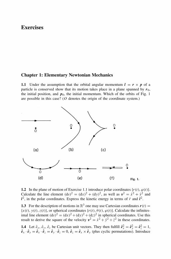
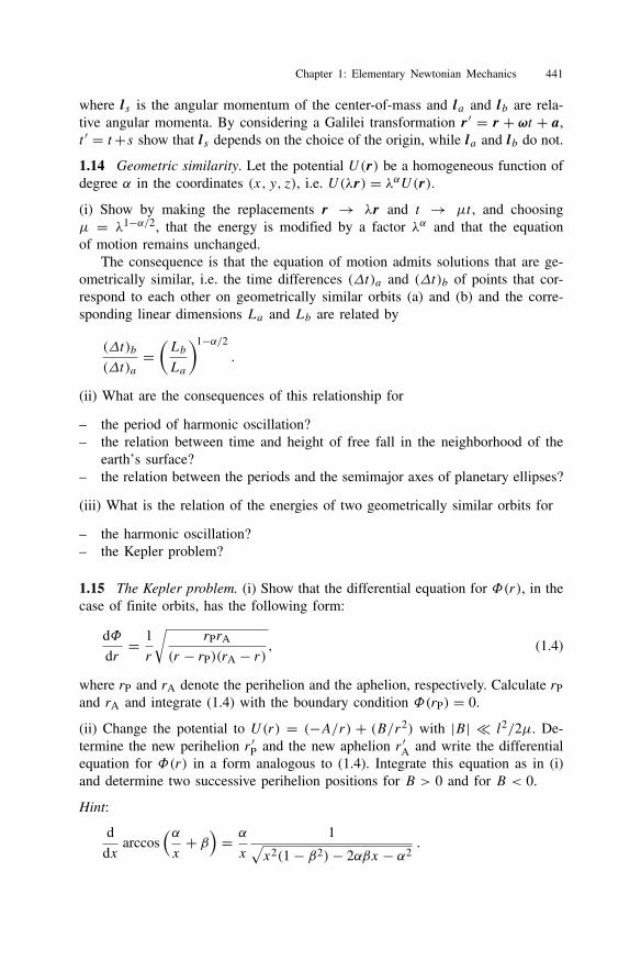
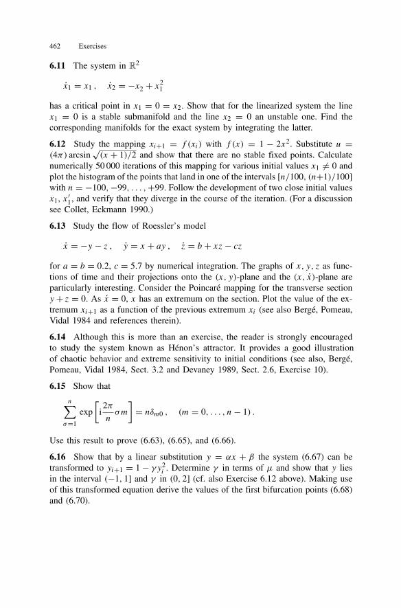
1.1 Under the assumption that the orbital angular momentum l = r × p of aparticle is conserved show that its motion takes place in a plane spanned by r0,the initial position, and p0, the initial momentum. Which of the orbits of Fig. 1are possible in this case? (O denotes the origin of the coordinate system.)
Fig. 1.
1.2 In the plane of motion of Exercise 1.1 introduce polar coordinates r(t), ϕ(t).Calculate the line element (ds)2 = (dx)2 + (dy)2, as well as v2 = x2 + y2 andl2, in the polar coordinates. Express the kinetic energy in terms of r and l2.
1.3 For the description of motions in R3 one may use Cartesian coordinates r(t) =x(t), y(t), z(t), or spherical coordinates r(t), θ(t), ϕ(t). Calculate the infinites-imal line element (ds)2 = (dx)2+ (dy)2+ (dz)2 in spherical coordinates. Use thisresult to derive the square of the velocity v2 = x2 + y2 + z2 in these coordinates.
1.4 Let ex , ey , ez be Cartesian unit vectors. They then fulfill e2x = e2
y = e2z = 1,
ex · ey = ex · ez = ey · ez = 0, ez = ex × ey (plus cyclic permutations). Introduce
438 Exercises
Fig. 2.
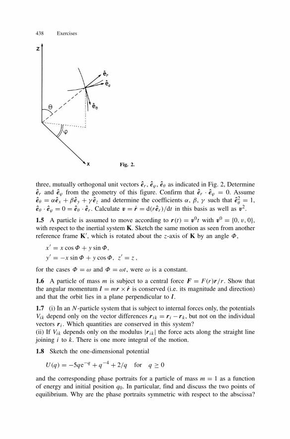
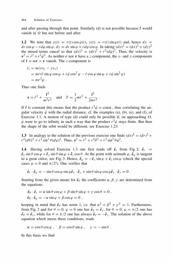
three, mutually orthogonal unit vectors er , eϕ , eθ as indicated in Fig. 2, Determineer and eϕ from the geometry of this figure. Confirm that er · eϕ = 0. Assumeeθ = αex + β ey + γ ez and determine the coefficients α, β, γ such that e2
θ = 1,eθ · eϕ = 0 = eθ · er . Calculate v = r = d(r er )/dt in this basis as well as v2.
1.5 A particle is assumed to move according to r(t) = v0t with v0 = 0, v, 0,with respect to the inertial system K. Sketch the same motion as seen from anotherreference frame K′, which is rotated about the z-axis of K by an angle Φ,
x′ = x cosΦ + y sinΦ,
y′ = −x sinΦ + y cosΦ, z′ = z ,for the cases Φ = ω and Φ = ωt , were ω is a constant.
1.6 A particle of mass m is subject to a central force F = F(r)r/r . Show thatthe angular momentum l = mr × r is conserved (i.e. its magnitude and direction)and that the orbit lies in a plane perpendicular to l.
1.7 (i) In an N -particle system that is subject to internal forces only, the potentialsVik depend only on the vector differences r ik = r i − rk , but not on the individualvectors r i . Which quantities are conserved in this system?(ii) If Vik depends only on the modulus |r ik| the force acts along the straight linejoining i to k. There is one more integral of the motion.
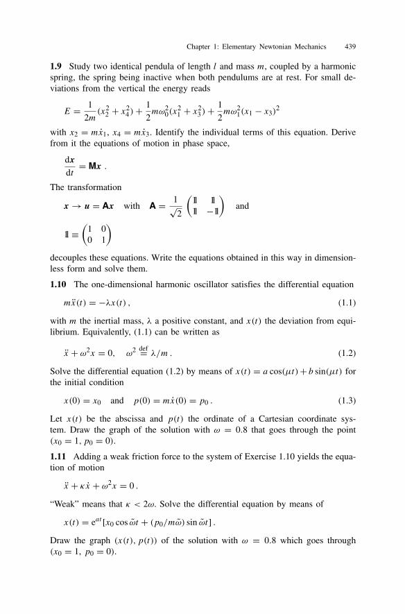
1.8 Sketch the one-dimensional potential
U(q) = −5qe−q + q−4 + 2/q for q ≥ 0
and the corresponding phase portraits for a particle of mass m = 1 as a functionof energy and initial position q0. In particular, find and discuss the two points ofequilibrium. Why are the phase portraits symmetric with respect to the abscissa?
Chapter 1: Elementary Newtonian Mechanics 439
1.9 Study two identical pendula of length l and mass m, coupled by a harmonicspring, the spring being inactive when both pendulums are at rest. For small de-viations from the vertical the energy reads
E = 1
2m(x2
2 + x24 )+
1
2mω2
0(x21 + x2
3 )+1
2mω2
1(x1 − x3)2
with x2 = mx1, x4 = mx3. Identify the individual terms of this equation. Derivefrom it the equations of motion in phase space,
dx
dt= Mx .
The transformation
x → u = Ax with A = 1√2
(1l 1l1l −1l
)and
1l ≡(
1 00 1
)decouples these equations. Write the equations obtained in this way in dimension-less form and solve them.
1.10 The one-dimensional harmonic oscillator satisfies the differential equation
mx(t) = −λx(t) , (1.1)
with m the inertial mass, λ a positive constant, and x(t) the deviation from equi-librium. Equivalently, (1.1) can be written as
x + ω2x = 0, ω2 def= λ/m . (1.2)
Solve the differential equation (1.2) by means of x(t) = a cos(µt)+ b sin(µt) forthe initial condition
x(0) = x0 and p(0) = mx(0) = p0 . (1.3)
Let x(t) be the abscissa and p(t) the ordinate of a Cartesian coordinate sys-tem. Draw the graph of the solution with ω = 0.8 that goes through the point(x0 = 1, p0 = 0).
1.11 Adding a weak friction force to the system of Exercise 1.10 yields the equa-tion of motion
x + κx + ω2x = 0 .
“Weak” means that κ < 2ω. Solve the differential equation by means of
x(t) = eat [x0 cos ωt + (p0/mω) sin ωt] .Draw the graph (x(t), p(t)) of the solution with ω = 0.8 which goes through(x0 = 1, p0 = 0).
440 Exercises
Fig. 3.
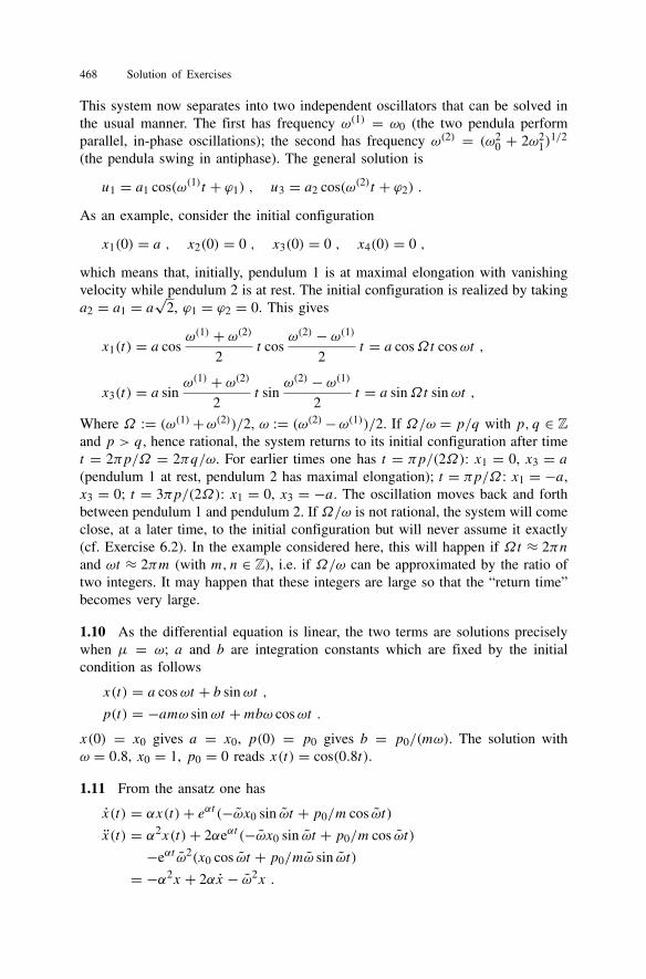
1.12 A mass point of mass m moves in the piecewise constant potential (seeFig. 3)
U =U1 f or x < 0
U2 f orx > 0.
In crossing from the domain x < 0, where its velocity was v1, to the domain x > 0,it changes its velocity (modulus and direction). Express U2 in terms of the quanti-ties U1, v1, α1, and α2. What is the relation of α1 to α2 when (i) U1 < U2 and (ii)U1 > U2 ? Work out the relationship to the law of refraction of geometrical optics.
Hint: Make use of the principle of energy conservation and show that one com-ponent of the momentum remains unchanged in crossing from x < 0 to x > 0.
Fig. 4.
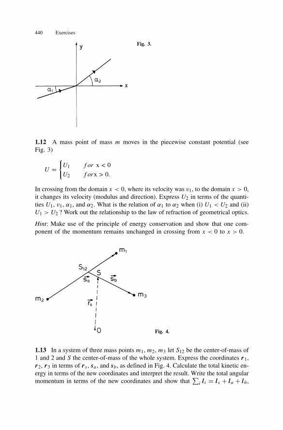
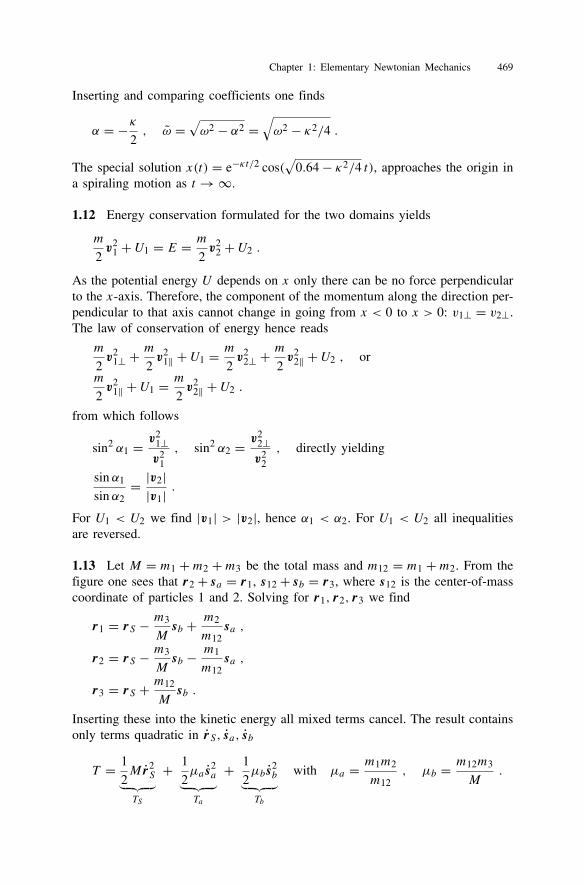
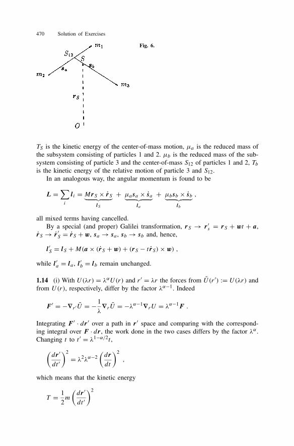
1.13 In a system of three mass points m1, m2, m3 let S12 be the center-of-mass of1 and 2 and S the center-of-mass of the whole system. Express the coordinates r1,r2, r3 in terms of rs , sa , and sb, as defined in Fig. 4. Calculate the total kinetic en-ergy in terms of the new coordinates and interpret the result. Write the total angularmomentum in terms of the new coordinates and show that
∑i li = ls + la + lb,
Chapter 1: Elementary Newtonian Mechanics 441
where ls is the angular momentum of the center-of-mass and la and lb are rela-tive angular momenta. By considering a Galilei transformation r ′ = r + ωt + a,t ′ = t+s show that ls depends on the choice of the origin, while la and lb do not.
1.14 Geometric similarity. Let the potential U(r) be a homogeneous function ofdegree α in the coordinates (x, y, z), i.e. U(λr) = λαU(r).(i) Show by making the replacements r → λr and t → µt , and choosingµ = λ1−α/2, that the energy is modified by a factor λα and that the equationof motion remains unchanged.
The consequence is that the equation of motion admits solutions that are ge-ometrically similar, i.e. the time differences (∆t)a and (∆t)b of points that cor-respond to each other on geometrically similar orbits (a) and (b) and the corre-sponding linear dimensions La and Lb are related by
(∆t)b
(∆t)a=
(Lb
La
)1−α/2.
(ii) What are the consequences of this relationship for
– the period of harmonic oscillation?– the relation between time and height of free fall in the neighborhood of the
earth’s surface?– the relation between the periods and the semimajor axes of planetary ellipses?
(iii) What is the relation of the energies of two geometrically similar orbits for
– the harmonic oscillation?– the Kepler problem?
1.15 The Kepler problem. (i) Show that the differential equation for Φ(r), in thecase of finite orbits, has the following form:
dΦ
dr= 1
r
√rPrA
(r − rP)(rA − r) , (1.4)
where rP and rA denote the perihelion and the aphelion, respectively. Calculate rPand rA and integrate (1.4) with the boundary condition Φ(rP) = 0.
(ii) Change the potential to U(r) = (−A/r) + (B/r2) with |B| l2/2µ. De-termine the new perihelion r ′P and the new aphelion r ′A and write the differentialequation for Φ(r) in a form analogous to (1.4). Integrate this equation as in (i)and determine two successive perihelion positions for B > 0 and for B < 0.
Hint:
d
dxarccos
(αx+ β
)= αx
1√x2(1− β2)− 2αβx − α2
.
442 Exercises
1.16 The most general solution of the Kepler problem reads, in terms of polarcoordinates r and Φ,
r(Φ) = p
1+ ε cos (φ − φ0).
The parameters are given by
p = l2
Aµ, (A = Gm1m2) ,
ε =√
1+ 2El2
µA2,
(µ = m1m2
m1 +m2
).
What values of the energy are possible if the angular momentum is given? Calcu-late the semimajor axis of the earth’s orbit under the assumption mSun mEarth;
G = 6.672× 10⁻¹¹ m3 kg−1 s−2 ,
mS = 1.989× 1030 kg ,
mE = 5.97× 1024 kg .
Calculate the semimajor axis of the ellipse along which the sun moves about thecenter-of-mass of the sun and the earth and compare the result to the solar radius(6.96× 10⁸ m).
1.17 Determine the interaction of two electric dipoles p1 and p2 (example fornoncentral potential force).
Hints: Calculate the potential of a single dipole p1, making use of the followingapproximation. The dipole consists of two charges ±e1 at a distance d1. Let e1tend to infinity and |d1| to zero, in such a way that their product p1 = d1e1 staysconstant. Then calculate the potential energy of a finite dipole p2 in the field ofthe first and perform the same limit e2 →∞, |d2| → 0, with p2 = d2e2 constant,as above. Calculate the forces that act on the two dipoles.
Answer:
W(1, 2) = (p1 · p2) /r3 − 3 (p1 · r) (p2 · r) /r5 ,
F = −∇1W = [3(p1 · p2)/r
5
−15(p1 · r)(p2 · r)/r7]r+3
[p1(p2 · r)+ p2(p1 · r)
]/r5 = −F 12 .
1.18 Let the motion of a point mass be governed by the law
v = v × a , a = const . (1.5)
Show that r · a = v(0) · a holds for all t and reduce (1.5) to an inhomogeneousdifferential equation of the form r + ω2r = f (t). Solve this equation by means
Chapter 1: Elementary Newtonian Mechanics 443
of the substitution rinhom(t) = ct + d. Express the integration constants in termsof the initial values r(0) and v(0). Describe the curve r(t) = rhom(t)+ r inhom(t).
Hint:
a1 × (a2 × a3) = a2(a1 · a3)− a3(a1 · a2) .
1.19 An iron ball falls vertically onto a horizontal plane from which it is reflected.At every bounce it loses the nth fraction of its kinetic energy. Discuss the orbitx = x(t) of the bouncing ball and derive the relation between xmax and tmax.
Hint: Study the orbit between two successive bounces and sum over previous times.
1.20 Consider the following transformations of the coordinate system:
t, r→Et, r, t, r→
Pt,−r, t, r→
T−t, r,
as well as the transformation P·T that is generated by performing first T and then P.Write these transformations in the form of matrices that act on the four-componentvector
(tr
). Show that E,P,T,PT form a group.
1.21 Let the potential U(r) of a two-body system be C2 (twice continuouslydifferentiable). For fixed relative angular momentum, under which additional con-dition on U(r) are there circular orbits? Let E0 be the energy of such an orbit.Discuss the motion for E = E0 + ε for small positive ε. Study the special cases
U(r) = rn and U(r) = λ/r .
1.22 Following the methods explained in Sect. 1.26 show the following.
(i) In the northern hemisphere a falling object experiences a southward deviationof second order (in addition to the first-order eastward deviation).
(ii) A stone thrown vertically upward falls down west of its point of departure, thedeviation being four times the eastward deviation of the falling stone.
1.23 Let a two-body system be subject to the potential
U(r) = − αr2
in the relative coordinate r , with positive α. Calculate the scattering orbits r(Φ).For fixed angular momentum what are the values of α for which the particle makesone (two) revolutions about the center of force? Follow and discuss an orbit thatcollapses to r = 0.
1.24 A pointlike comet of mass m moves in the gravitational field of a sun withmass M and radius R. What is the total cross section for the comet to crash onthe sun?
444 Exercises
1.25 Solve the equations of motion for the example of Sect. 1.21.2 (Lorentz forcewith constant fields) for the case
B = B ez , E = Eez .
Chapter 2: The Principles of Canonical Mechanics
2.1 The energy E(q, p) is an integral of a finite, one-dimensional, periodic mo-tion. Why is the portrait symmetric with respect to the q-axis? The surface enclosedby the periodic orbit is
F(E) =∮p dq = 2
∫ qmax
qmin
p dq .
Show that the change of F(E) with E equals the period T of the orbit, T =dF(E)/dE, Calculate F and T for the example
E(q, p) = p2/2m+mω2q2/2 .
2.2 A weight glides without friction along a plane inclined by the angle α withrespect to the horizontal. Study this system by means of d’Alembert’s principle.
2.3 A ball rolls without friction on the inside of a circular annulus. The annulusis put upright in the earth’s gravitational field. Use d’Alembert’s principle to derivethe equation of motion and discuss its solutions.
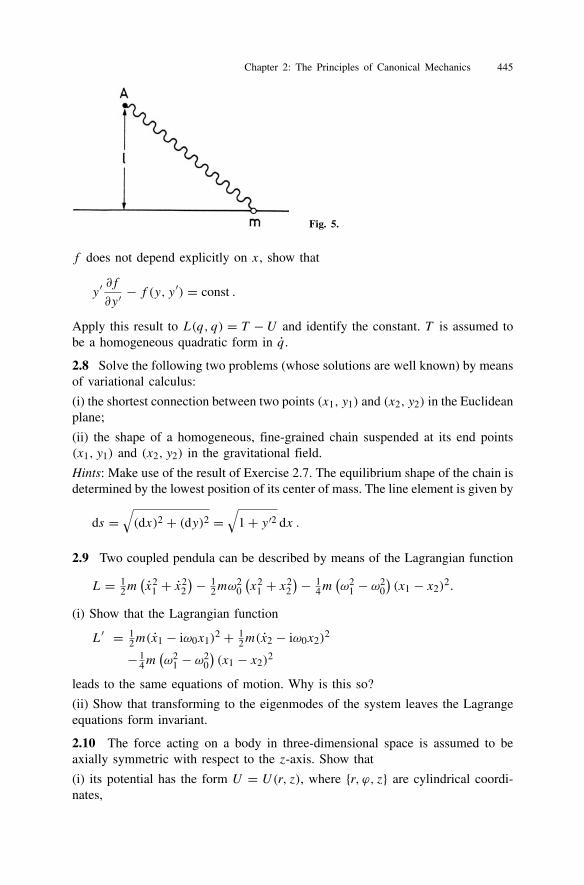
2.4 A mass point m that can only move along a straight line is tied to the pointA by means of a spring. The distance of A to the straight line is l (cf. Fig. 5).Calculate (approximately) the frequency of oscillation of the mass point.
2.5 Two equal masses m are connected by means of a (massless) spring withspring constant x. They move without friction along a rail, their distance beingl when the spring is inactive. Calculate the deviations x1(t) and x2(t) from theequilibrium positions, for the following initial conditions:
x1(0) = 0 , x1(0) = v0,
x2(0) = l , x2(0) = 0.
2.6 Given a function F(x1, . . . , xf ) that is homogeneous and of degree N in itsf variables, show that
f∑i=1
∂F
∂xixi = NF .
2.7 If in the integral
I [y] =∫ x2
x1
dx f (y, y′)
Chapter 2: The Principles of Canonical Mechanics 445
Fig. 5.
f does not depend explicitly on x, show that
y′ ∂f∂y′
− f (y, y′) = const .
Apply this result to L(q, q) = T − U and identify the constant. T is assumed tobe a homogeneous quadratic form in q.
2.8 Solve the following two problems (whose solutions are well known) by meansof variational calculus:
(i) the shortest connection between two points (x1, y1) and (x2, y2) in the Euclideanplane;
(ii) the shape of a homogeneous, fine-grained chain suspended at its end points(x1, y1) and (x2, y2) in the gravitational field.
Hints: Make use of the result of Exercise 2.7. The equilibrium shape of the chain isdetermined by the lowest position of its center of mass. The line element is given by
ds =√(dx)2 + (dy)2 =
√1+ y′2 dx .
2.9 Two coupled pendula can be described by means of the Lagrangian function
L = 12m
(x2
1 + x22
)− 12mω
20
(x2
1 + x22
)− 14m
(ω2
1 − ω20
)(x1 − x2)
2.
(i) Show that the Lagrangian function
L′ = 12m(x1 − iω0x1)
2 + 12m(x2 − iω0x2)
2
− 14m
(ω2
1 − ω20
)(x1 − x2)
2
leads to the same equations of motion. Why is this so?
(ii) Show that transforming to the eigenmodes of the system leaves the Lagrangeequations form invariant.
2.10 The force acting on a body in three-dimensional space is assumed to beaxially symmetric with respect to the z-axis. Show that
(i) its potential has the form U = U(r, z), where r, ϕ, z are cylindrical coordi-nates,
446 Exercises
x = r cosϕ , y = r sin ϕ , z = z ;(ii) the force always lies in a plane containing the z-axis.
2.11 With respect to an inertial system K0 the Lagrangian function of a particle is
L0 = 12mx2
0 − U(x0) .
The frame of reference K has the same origin as K0 but rotates about the latterwith constant angular velocity ω. Show that the Lagrangian with respect to K reads
L = mx2
2+mx · (ω × x)+ m
2(ω × x)2 − U(x) .
Derive the equations of motion of Sect. 1.25 from this.
2.12 A planar pendulum is suspended such that its point of suspension glideswithout friction along a horizontal axis. Construct the kinetic and potential en-ergies and a Lagrangian function for this problem.
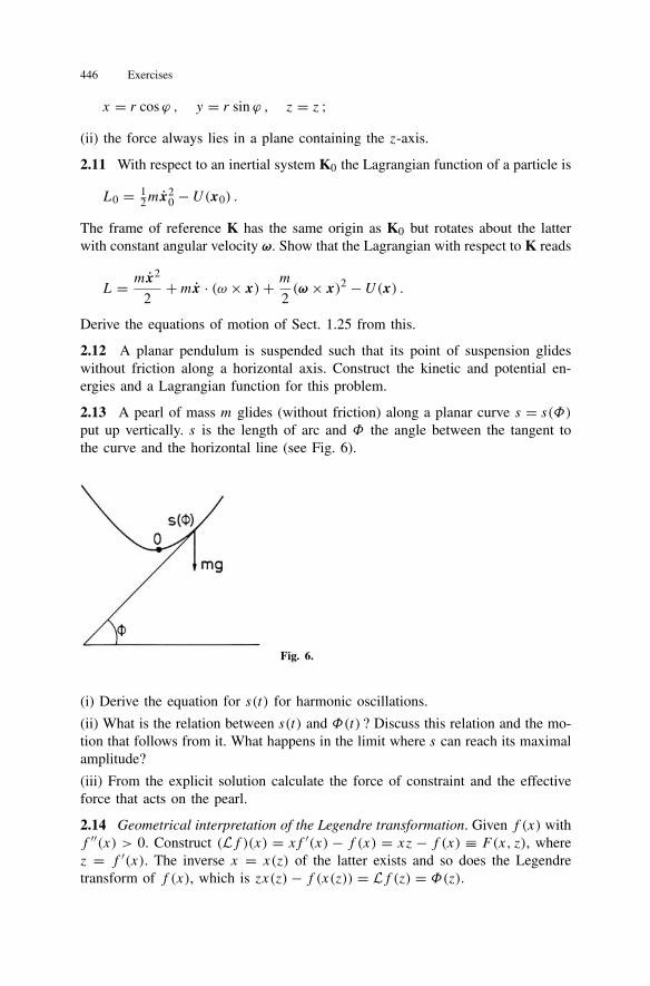
2.13 A pearl of mass m glides (without friction) along a planar curve s = s(Φ)put up vertically. s is the length of arc and Φ the angle between the tangent tothe curve and the horizontal line (see Fig. 6).
Fig. 6.
(i) Derive the equation for s(t) for harmonic oscillations.
(ii) What is the relation between s(t) and Φ(t) ? Discuss this relation and the mo-tion that follows from it. What happens in the limit where s can reach its maximalamplitude?
(iii) From the explicit solution calculate the force of constraint and the effectiveforce that acts on the pearl.
2.14 Geometrical interpretation of the Legendre transformation. Given f (x) withf ′′(x) > 0. Construct (Lf )(x) = xf ′(x) − f (x) = xz − f (x) ≡ F(x, z), wherez = f ′(x). The inverse x = x(z) of the latter exists and so does the Legendretransform of f (x), which is zx(z)− f (x(z)) = Lf (z) = Φ(z).

Chapter 2: The Principles of Canonical Mechanics 447
(i) Comparing the graphs of the functions y = f (x) and y = zx (for fixed z) onesees with
∂F (x, z)
∂x= 0
that x = x(z) is the point where the vertical distance between the two graphs ismaximal (see Fig. 7).
Fig. 7.
(ii) Take the Legendre transform of Φ(z), i.e. (LΦ)(z) = zΦ ′(z) − Φ(z) =zx − Φ(z) ≡ G(z, x) with Φ ′(z) = x. Identify the straight line y = G(z, x)
for fixed z and with x = x(z) and show that one has G(z, x) = f (x). Sketch thepicture that one obtains if one keeps x = x0 fixed and varies z.
2.15 (i) Let
L(q1, q2, q1, q2, t) = T − U with
T =2∑
i,k=1
cikqi qk +2∑k=1
bkqk + a .
Under what condition can one construct H(q˜, p˜, t) and what are p1, p2, and H ?
Confirm that the Legendre transform of H is again L and that
det
(∂2L
∂qk∂qi
)det
(∂2H
∂pn∂pm
)= 1 .
Hint: Take d11 = 2c11, d12 = d21 = c12 + c21, d22 = 2c22, πi = pi − bi .(ii) Assume now that L = L(x1 ≡ q1, x2 ≡ q2, q1, q2, t) ≡ L(x1, x2,u) with
udef= (q1, q2, t) to be an arbitrary Lagrangian function. We expect the momenta
pi = pi(x1, x2,u) derived from L to be independent functions of x1 and x2, i.e.that there is no function F(p1(x1, x2,u), p2(x1, x2,u)) that vanishes identically.
448 Exercises
Show that, if p1 and p2 were dependent, the determinant of the second derivativesof L with respect to the xi would vanish.
Hint: Consider dF/dx1 and dF/dx2.
2.16 A particle of mass m is described by the Lagrangian function
L = 1
2m(x2 + y2 + z2)+ ω
2l3 ,
where l3 is the z-component of angular momentum and ω is a constant frequency.Find the equations of motion, write them in terms of the complex variable x + iyand of z, and solve them. Construct the Hamiltonian function and find the kine-matical and canonical momenta. Show that the particle has only kinetic energyand that the latter is conserved.
2.17 Invariance under time translations and Noether’s theorem. The theorem ofE. Noether can be applied to the case of translations in time by means of the fol-lowing trick. Make t a coordinate-like variable by parametrizing both q and t byq = q(τ), t = t (τ ) and by defining the following Lagrangian function:
L
(q, t,
dq
dτ,
dt
dτ
)def= L
(q,
1
dt/dτ
dq
dτ, t
)dt
dτ.
(i) Show that Hamilton’s variational principle applied to L yields the same equa-tions of motion as for L.
(ii) Assume L to be invariant under time translations
hs(q, t) = (q, t + s) . (2.1)
Apply Noether’s theorem to L and find the constant of the motion correspondingto the invariance (2.1).
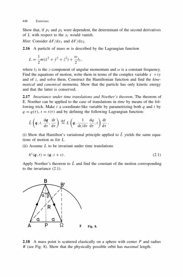
Fig. 8.
2.18 A mass point is scattered elastically on a sphere with center P and radiusR (see Fig. 8). Show that the physically possible orbit has maximal length.
Chapter 2: The Principles of Canonical Mechanics 449
Hints: Show first that the angles α and β must be equal and construct the actionintegral. Show that any other path AB ′Ω would be shorter than for those pointswhere the sum of the distances to A and Ω is constant and equal to the length ofthe physical orbit.
2.19 (i) Show that canonical transformations leave the physical dimension of theproduct piqi unchanged, i.e. [PiQi] = [piqi]. Let Φ be the generating functionfor a canonical transformation. Show that
[piqi] = [PkQk] = [Φ] = [H · t] ,where H is the Hamiltonian function and t the time.
(ii) In the Hamiltonian function H = p2/2m+mω2q2/2 of the harmonic oscillatorintroduce the variables
x1def= ω√mq , x2
def= p/√m, τdef= ωt ,
thus obtaining H = (x21 + x2
2 )/2. What is the generating function Φ(x1, y1) forthe canonical transformation x →
Φ
y that corresponds to the function Φ(q,Q) =(mωq2/2) cotQ ? Calculate the matrix Mik = ∂xi/∂yk and confirm det M = 1and MTJM = J.
2.20 The group Sp2f is particularly simple for f = 1, i.e. in two dimensions.
(i) Show that every matrix
M =(a11 a12a21 a22
)is symplectic if and only if a11a22 − a12a21 = 1.
(ii) Therefore, the orthogonal matrices
O =(
cosα sin α− sin α cosα
)and the symmetric matrices
S =(x y
y z
)with xz− y2 = 1
belong to Sp2f . Show that every M ∈ Sp2f can be written as a product
M = S ·Oof a symmetric matrix S with determinant 1 and an orthogonal matrix O.
2.21 (i) Evaluate the following Poisson brackets for a single particle:
li , rk , li , pk , li , r , li ,p2 .
450 Exercises
(ii) If the Hamiltonian function in its natural form H = T +U is invariant underrotations, what quantities can U depend on?
2.22 Making use of the Poisson brackets show that for the system H = T +U(r)with U(r) = γ /r and γ a constant, the vector
A = p × l + xmγ/r
is an integral of the motion (Lenz’ vector or Hermann–Bernoulli–Laplace vector).
2.23 The motion of a particle of mass m is described by
H = 1
2m
(p2
1 + p22
)+mαq1 , α = const .
Construct the solution of the equations of motion for the initial conditions
q1(0) = x0 , q2(0) = y0 , p1(0) = px , p2(0) = py ,making use of Poisson brackets.
2.24 For a three-body system with masses mi , coordinates r i , and momenta piintroduce the following coordinates (Jacobian coordinates2):
ϕ1def= r2 − r1 (relative coordinate of particles 1 and 2) ,
ϕ2def= r3 − m1r1 +m2r2
m1 +m2(relative coordinate of particle 3
and the center of mass of the first two) ,
ϕ3def= m1r1 +m2r2 +m3r3
m1 +m2 +m3(center of mass of the three particles) ,
π1def= m1p2 −m2p1
m1 +m2,
p2def= (m1 +m2)p3 −m3(p1 + p2)
m1 +m2 +m3,
π3def= p1 + p2 + p3 .
(i) What is the physical interpretation of the momenta π1, π2, π3 ?
(ii) How would you define such coordinates for four or more particles?
(iii) Show in at least two (equivalent) ways that the transformation
r1, r2, r3,p1,p2,p3 → ϕ1,ϕ2,ϕ3,π1,π2,π3is canonical.
2.25 Given a Lagrangian function L for which ∂L/∂t = 0, study only those varia-tions of the orbits qk(t, α) which belong to a fixed energy E =∑
k qk(∂L/∂qk)−L2 Jacobi, C.G.J., Sur l’élimination des noeuds dans le problème des trois corps, Crelles Journal für
reine und angewandte Mathematik, XXVI (1843) 115
Chapter 2: The Principles of Canonical Mechanics 451
and whose end points are kept fixed irrespective of the time (t2−t1) that the systemneeds to move from the initial to the end point, i.e.
qk(t, α) with
qk(t1(α), α) = q(1)kqk(t2(α), α) = q(2)k
for all α . (2.1)
Thus, initial and final times are also varied, ti = ti (α).(i) Calculate the variation of I (α),
δI = dI (α)
dα
∣∣∣∣α=0
dα =∫ t2(α)
t1(α)
L(qk(t, α), qk(t, α)) dt . (2.2)
(ii) Show that the variational principle
δK = 0 with Kdef=
∫ t2
t1
(L+ E) dt
together with the prescriptions (2.1) is equivalent to the Lagrange equations (thePrinciple of Euler and Maupertuis).
2.26 The kinetic energy
T =f∑
i,k=1
qikqi qk = 1
2(L+ E)
is assumed to be a positive symmetric quadratic form in the qi . The orbit in thespace spanned by the qk is described by the length of arc s such that T = (ds/dt)2.With E = T + U the integral K of Exercise 2.25 can be replaced with an inte-gral over s. Show that the integral principle obtained in this way is equivalent toFermat’s principle of geometric optics,
δ
∫ x2
x1
n(x, ν) ds = 0
(n: index of refraction, ν: frequency).
2.27 LetH = p2/2+U(q), where the potential is such that it has a local minimumat q0. Thus, in an interval q1 < q0 < q2 the potential forms a potential well. Sketcha potential with this property and show that there is an interval U(q0) < E ≤ Emaxwhere there are periodic orbits. Consider the characteristic equation of Hamiltonand Jacobi (2.154). If S(q,E) is a complete integral then t − t0 = ∂S/∂E. Takethe integral
I (E)def= 1
2π
∮ΓE
p dq
over the periodic orbit ΓE with energy E (this is the surface enclosed by ΓE).Write I (E) as an integral over time and show that
dI
dE= T (E)
2π.
452 Exercises
2.28 In Exercise 2.27 replace S(q,E) by S(q, I ) with I = I (E) as defined there.S generates the canonical transformation (q, p,H) → (θ, I, H = E(Ω)). Whatare the canonical equations in the new variables? Can they be integrated?
2.29 Let H 0 = p2/2+q2/2. Calculate the integral I (E) defined in Exercise 2.27.Solve the characteristic equation of Hamilton and Jacobi (2.154) and write the so-lution as S(q, I ). Then θ = ∂S/∂I . Show that (q, p) and (θ, I ) are related by thecanonical transformation (2.95) of Sect. 2.24 (ii).
2.30 We assume that the Lagrangian of a mechanical system with one degree offreedom does not depend explicitly on time. In Hamilton’s variational principle wemake a smooth change of the end points qa and qb, as well as of the running timet = t2−t1, in the sense that the solution ϕ(t) for the values (qa, qb, t) and the solu-tion φ(s, t) which belongs to the values (q ′a, q ′b, t ′) are related in a smooth man-ner: ϕ(t) → φ(s, t) such that φ(s, t) is differentiable in s and φ(s = 0, t) = ϕ(t).
Show that the corresponding change of the action integral I0 into which thephysical solution is inserted (this function is called Hamilton’s principal function),is given by the following expression
δI0 = −E δt + pb δqb − pa δqa .
Chapter 3: The Mechanics of Rigid Bodies
3.1 Let two systems of reference K and K be fixed in the center of mass of arigid body, the axes of the former being fixed in space, those of the latter fixed inthe body. If J is the inertia tensor with respect to K and J the one as calculatedin K, show that (i) J and J have the same eigenvalues. (Use the characteristicpolynomial.)
(ii) K is now assumed to be a system of principal axes of inertia. What is the formof J? Calculate J for the case of rotation of the body about the 3-axis.
3.2 Two particles with masses m1 and m2 are held by a rigid but massless straightconnection with length l. What are the principal axes and what are the momentsof inertia?
3.3 The inertia tensor of a rigid body is found to have the form
Iik =⎛⎝I11 I12 0I21 I22 00 0 I33
⎞⎠ , I21 = I12 .
Determine the three moments of inertia and consider the following special cases.
(i) I11 = I22 = A, I12 = B. Can I33 be arbitrary?
(ii) I11 = A, I22 = 4A, I12 = 2A. What can you say about I33? What is the shapeof the body in this example?
Chapter 3: The Mechanics of Rigid Bodies 453
Fig. 9.
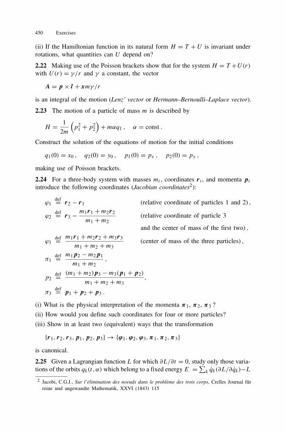
3.4 Construct the Lagrangian function for general, force-free motion of a conicaltop (height h, massM , radius of base circle R). What are the equations of motion?Are there integrals of the motion and what is their physical interpretation?
3.5 Calculate the moments of inertia of a torus filled homogeneously with mass.Its main radius is R; the radius of its section is r .
3.6 Calculate the moment of inertia I3 for two arrangements of four balls, twoheavy (radius R, mass M) and two light (radius r , mass m) with homogeneousmass density, as shown in Fig. 9. As a model of a dancer’s pirouette compare theangular velocity for the two arrangements, with L3 fixed and equal in the two cases.
3.7 (i) Let the boundary of a homogeneous body be defined by the formula (inspherical coordinates)
R(θ) = R0(1+ α cos θ) ,
i.e. (r, θ,Φ) = 0 = const for r ≤ R(θ) and all θ and Φ, and (r, θ,Φ) = 0for r > R(θ). If M is the total mass, calculate 0 and the moments of inertia.
(ii) Perform the same calculation for a homogeneous body whose shape is given by
R(θ) = R0(1+ βY20(θ))
with Y20(θ) = √5/16π(3 cos2 θ − 1) being the spherical harmonic with l = 2,
m = 0. In both examples sketch the body.
3.8 Determine the moments of inertia of a rigid body whose inertia tensor withrespect to a system of reference K1 (fixed in the body) is given by
J =
⎛⎜⎜⎜⎜⎜⎝9
8
1
4
−√3
81
4
3
2
−√3
4−√3
8
−√3
4
11
8
⎞⎟⎟⎟⎟⎟⎠ .
454 Exercises
Fig. 10.
Can one indicate the relative position of the principal inertia system K0 relativeto K1 ?
3.9 A ball with radius a is filled homogeneously with mass such that the densityis 0. The total mass is M .
(i) Write the mass density with respect to a body-fixed system centered inthe center of mass and express 0 in terms of M . Let the ball rotate about a pointP on its surface (see Fig. 10).
(ii) What is the same density function (r, t) as seen from a space-fixed systemcentered on P ?
(iii) Give the inertia tensor in the body-fixed system of (i). What is the momentof inertia for rotation about a tangent to the ball in P ?
Hint: Use the step function Θ(x) = 1 for x ≥ 0, Θ(x) = 0 for x < 0.
3.10 A homogeneous circular cylinder with length h, radius r , and mass m rollsalong an inclined plane in the earth’s gravitational field.
(i) Construct the full kinetic energy of the cylinder and find the moment of inertiarelevant to the described motion.
(ii) Construct the Lagrangian function and solve the equation of motion.
3.11 Manifold of motions of the rigid body. A rotation R ∈ SO(3) can be deter-mined by a unit vector ϕ (the direction about which the rotation takes place) andan angle ϕ.
(i) Why is the interval 0 ≤ ϕ ≤ π sufficient for describing every rotation?
(ii) Show that the parameter space (ϕ, ϕ) fills the interior of a sphere with radiusπ in R3. This ball is denoted by D3. Confirm that antipodal points on the ball’ssurface represent the same rotation.
(iii) There are two types of closed orbit in D3, namely those which can be con-tracted to a point and those which connect two antipodal points. Show by meansof a sketch that every closed curve can be reduced by continuous deformation toeither the former or the latter type.
3.12 Calculate the Poisson brackets (3.92–95).
Chapter 4: Relativistic Mechanic 455
Chapter 4: Relativistic Mechanics
4.1 (i) A neutral π meson (π0) has constant velocity v0 along the x3-direction.Write its energy-momentum vector. Construct the special Lorentz transformationthat leads to the particle’s rest system.
(ii) The particle decays isotropically into two photons, i.e. with respect to its restsystem the two photons are emitted in all directions with equal probability. Studytheir decay distribution in the laboratory system.
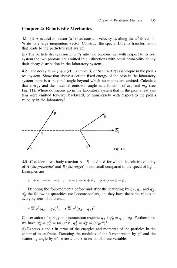
4.2 The decay π → µ+ν (cf. Example (i) of Sect. 4.9.2) is isotropic in the pion’srest system. Show that above a certain fixed energy of the pion in the laboratorysystem there is a maximal angle beyond which no muons are emitted. Calculatethat energy and the maximal emission angle as a function of mπ and mµ (seeFig. 11). Where do muons go in the laboratory system that in the pion’s rest sys-tem were emitted forward, backward, or transversely with respect to the pion’svelocity in the laboratory?
Fig. 11.
4.3 Consider a two-body reaction A+B → A+B for which the relative velocityof A (the projectile) and B (the target) is not small compared to the speed of light.Examples are
e− + e+ → e− + e− , ν + e → e+ ν , p+ p → p+ p .
Denoting the four-momenta before and after the scattering by qA, qB and q ′A,q ′B the following quantities are Lorentz scalars, i.e. they have the same values inevery system of reference,
sdef= c2(qA + qB)2 , t
def= c2(qA − q ′A)2 .Conservation of energy and momentum requires q ′A+q ′B = qA+qB . Furthermore,we have q2
A = q ′2A = (mAc2)2, q2B = q ′2B = (mBc2)2.
(i) Express s and t in terms of the energies and momenta of the particles in thecenter-of-mass frame. Denoting the modulus of the 3-momentum by q∗ and thescattering angle by θ∗, write s and t in terms of these variables.
456 Exercises
(ii) Define u = c2(qA − q ′B)2 and show that
s + t + u = 2(m2A +m2
B
)c4 .
4.4 Calculate the variables s and t (as defined in Exercise 4.3) in the labora-tory system, i.e. in that system where B is at rest before the scattering. What isthe relation between the scattering angle θ in the laboratory system and θ∗ in thecenter-of-mass frame? Compare to the nonrelativistic expression (1.80).
4.5 In its rest system the electron’s spin is described by the 4-vector sα = (0, s).What is the form of this vector in a frame where the electron has the momentump? Calculate the scalar product (s · p) = sαpα .
4.6 Show that
(i) every lightlike vector z (z2 = 0) can be brought to the form (1,1,0,0) by meansof Lorentz transformations;
(ii) every spacelike vector can be transformed to the form (0, z1, 0, 0), wherez1 = √−z2.
Indicate the necessary transformations in both cases.
4.7 If Ji and Ki denote the generators of rotations and boosts, respectively (cf.Sect. 4.5.2 (iii)) define
Apdef= 1
2
(Jp + iKp
), Bq
def= 1
2
(Jq − iKq
), p, q = 1, 2, 3 .
Making use of the commutation rules (4.59) calculate [Ap,Aq ], [Bp,Bq ], and[Ap,Bq ] and compare to (4.59).
4.8 Study the behavior of Ji and Kj with respect to space inversion, i.e. determinePJiP−1, PKj P−1.
4.9 In quantum theory one prefers to use the quantities
Jidef= iJi , Kj
def= − iKj .
What are the commutators (4.59) for these matrices? Show that the matrices Ji
are Hermitian, i.e. that (JTi )∗ = Ji .
4.10 A muon decays predominantly into an electron and two nearly massless neu-trinos, µ− → e−+ν1+ν2. If the muon is at rest, show that the electron assumes itsmaximal momentum whenever the neutrinos are emitted parallel to each other. Cal-culate the maximal and minimal energies of the electron as functions ofmµ andme.
Answer:
Emax =m2µ +m2
e
2mµc2 , Emin = mec
2 .
Draw the corresponding momenta in the two cases.
Chapter 4: Relativistic Mechanic 457
4.11 A particle of mass M is assumed to decay into three particles (1,2,3) withmasses m1, m2, m3. Determine the maximal energy of particle 1 in the rest systemof the decaying particle as follows. Set
p1 = −f (x)n , p2 = xf (x)n , p3 = (1− x)f (x)n ,where n is a unit vector and x is a number between 0 and 1. Find the maximumof f (x) from the principle of energy conservation.
Examples:
(i) µ− → e− + ν1 + ν2 (cf. Exercise 4.10),
(ii) Neutron decay: n → p+ e+ ν.
What is the maximal energy of the electron? What is the value of β = |v|/c forthe electron? mn −mp = 2.53me, mp = 1836me.
4.12 Pions π+, π− have the mean lifetime τ 2.6× 10⁻⁸ s and decay predom-inantly into a muon and a neutrino. Over what distance can they fly, on average,before decaying if their momentum is pπ = x · mπc with x = 1, 10, or 1000?(mπ 140 MeV/c2 = 2.50× 10⁻²⁸ kg).
4.13 The free neutron is unstable. Its mean lifetime is τ 900 s. How far can aneutron fly on average if its energy is E = 10−2mnc
2 or E = 1014mnc2 ?
4.14 Show that a free electron cannot radiate a single photon, i.e. the process
e → e+ γcannot take place because of energy and momentum conservation.
4.15 The following transformation
I : xµ → xµ = R2
x2xµ
implies the relation√x2√x2 = R2. This is an obvious generalization of the well-
known inversion at the circle of radius R, r · r = R2. Show that the sequence oftransformations: inversion I of xµ, translation T of the image by the vector R2cµ,and another inversion of the result, i.e.,
x′ = (I T I)x
is precisely the special conformal transformation (4.102).
4.16 Consider the following Lagrangian
L = 1
2m
(ψ q2 − c2
0(ψ − 1)2
ψ
)≡ L(q, ψ)
which contains the additional, dimensionless, degree of freedom ψ . The parameterc0 has the physical dimension of a velocity. Show: The extremum of the actionintegral yields a theory obeying special relativity for which c0 is the maximal ve-locity, in other words, one obtains the Lagrangian (4.97) with the velocity of lightc replaced by c0. Consider the limit c0 →∞.
458 Exercises
Chapter 5: Geometric Aspects of Mechanics
5.1 Letkω be an exterior k-form,
lω an exterior l-form. Show that their exterior
product is symmetric if k and/or l are even and antisymmetric if both are odd, i.e.
kω∧ l
ω = (−1)k·l lω∧ kω .
5.2 Let x1, x2, x3 be local coordinates in the Euclidean space R3, ds2 = E1 dx21+
E2 dx22 +E3 dx2
3 the square of the line element, and e1, e2, e3 unit vectors alongthe coordinate directions. What is the value of dxi(ej ), i.e. of the action of theone-form dxi on the unit vector ej ?
5.3 Let a =∑3i=1 ai(x)ei be a vector field with ai(x) smooth functions onM . To
every such vector field we associate a one-form1ωa and a two-form
2ωa such that
1ωa(ξ) = (a · ξ) , 2
ωa(ξ , η) = (a · (ξ × η)) .
Show that
1ωa =
3∑i=1
ai(x)√Ei dxi ,
2ωa = ai(x)
√E2E3 dx2 ∧ dx3 + cyclic permutations ,
5.4 Making use of the results of Exercise 5.3 determine the components of ∇fin the basis e1, e2, e3Answer:
∇f =3∑i=1
1√Ei
∂f
∂xiei .
5.5 Determine the functions Ei for the case of Cartesian, cylindrical, and sphericalcoordinates. In each case give the components of ∇f .
5.6 To the force F = (F1, F2) in the plane we associate the one-form ω =F1 dx1+F2 dx2. When we apply ω onto a displacement vector, ω(ξ) is the workdone by the force. What is the dual ∗ω of the form ω ? What is its interpretation?
5.7 The Hodge star operator assigns to every k-form ω the (n−k)-form ∗ω. Showthat
∗(∗ω) = (−1)k·(n−k)ω .
Chapter 5: Geometric Aspects of Mechanics 459
5.8 Let E = (E1, E2, E3) and B = (B1, B2, B3) be electric and magnetic fieldsthat in general depend on x and t . We assign the following exterior forms to them:
ϕdef=
3∑i=1
Eidxi ,
ωdef= B1 dx2 ∧ dx3 + B2 dx3 ∧ dx1 + B3 dx1 ∧ dx2 .
Write the homogeneous Maxwell equation curl E + B/c = 0 as an equation be-tween the forms ϕ and ω.
5.9 If d denotes the exterior derivatives and ∗ the Hodge star operator, the cod-ifferential δ is defined by
δdef= ∗ d ∗ .
Show that ∆def= d δ+ δ d, when applied to functions, is the Laplacian operator
∆ =∑i
∂2
∂xi2.
5.10 Let
kω =
∑i1<···<ik
ωi1...ik (x˜ ) dxi1 ∧ · · · ∧ dxik
be an exterior k-form over a vector space W . Let F : V → W be a smooth
mapping of the vector space V onto W . Show that the pull-back F ∗( kω∧ lω) of the
exterior product of two such forms is equal to the exterior product of the pull-back
of the individual forms (F ∗ kω) ∧ (F ∗ lω).5.11 With the same assumptions as in Exercise 5.10 show that the exterior deriva-tive and the pull-back commute,
d(F ∗ω) = F ∗(dω) .
5.12 Let x and y be Cartesian coordinates in R2, V = y∂x and W = x∂y twovector fields on R2. Calculate the Lie bracket [V,W ]. Sketch the vector fields V,W , and [V,W ] along circles about the origin.
5.13 Prove the follow assertions.
(i) The set of all tangent vectors to the smooth manifold M at the point p ∈ Mform a real vector space, denoted by TpM , whose dimension is n = dimM .
(ii) If M is Rn, TpM is isomorphic to that space.
460 Exercises
5.14 The canonical two-form for a system with two degrees of freedom readsω = ∑2
i=1 dqi ∧ dpi . Calculate ω ∧ ω and confirm that this product is propor-tional to the oriented volume element in phase space.
5.15 Let H(1) = p2/2 + (1 − cos q) and H(2) = p2/2 + q(q2 − 3)/6 be theHamiltonian functions for two systems with one degree of freedom. Construct thecorresponding Hamiltonian vector fields and sketch them along some of the solu-tion curves.
5.16 Let H = H 0 +H ′ with H 0 = (p2 + q2)/2 and H ′ = εq3/3. Construct theHamiltonian vector fields XH 0 and XH and calculate ω(XH ,XH 0).
5.17 Let L and L′ be two Lagrangian functions on TQ for which ΦL and ΦL′are regular. The corresponding vector fields and canonical two-forms are XE , XE′ ,ωL, and ωL′ . Show that each of the following assertions implies the other:
(i) L′ = L+ α, where α: TQ→ R is a closed one-form, i.e. dα = 0;
(ii) XE = XE′ and ωL = ωL′ .Show that in local coordinates this is the result obtained in Sect. 2.10.
Chapter 6: Stability and Chaos
6.1 Study the two-dimensional linear system y˜= Ay
˜, where A has one of the
Jordan normal forms
(i) A =(λ1 00 λ2
), (ii) A =
(a b
−b a
), (iii) A =
(λ 01 λ
).
In all three cases determine the characteristic exponents and the flow (6.13) withs = 0. Suppose the system is obtained by linearizing a dynamical system in theneighborhood of an equilibrium position. (i) corresponds to the situations shownin Figs. 6.2a–c. Draw the analogous pictures for (ii) for (a = 0, b > 0) and(a < 0, b > 0), and for (iii) with λ < 0.
6.2 The variables α and β on the torus T 2 = S1×S1 define the dynamical system
α = a/2π , β = b/2π , 0 ≤ α, β ≤ 1 ,
where a and b are real constants. Cutting the torus at (α = 1, β) and at (α, β = 1)yields a square of length 1. Draw the solutions with initial condition (α0, β0) inthis square for b/a rational and irrational.
6.3 Show that in an autonomous Hamiltonian system with one degree of freedom(and hence two-dimensional phase space) neighboring trajectories can diverge atmost linearly with increasing time as long as one keeps clear from saddle points.
Hint: Make use of the characteristics equation (2.154) of Hamilton and Jacobi.
6.4 Study the system
Chapter 6: Stability and Chaos 461
q1 = −µq1 − λq2 + q1q2
q2 = λq1 − µq2 +(q2
1 − q22
)/2 ,
where 0 ≤ µ 1 is a damping term and λ with |λ| 1 is a detuning parameter.Show that if µ = 0 the system is Hamiltonian. Find a Hamiltonian function for thiscase. Draw the projection of its phase portraits for λ > 0 onto the (q1, q2)-planeand determine the position and the nature of the critical points.
Show that the picture obtained above is structurally unstable when µ is chosento be different from zero and positive, by studying the change of the critical pointsfor µ = 0.
6.5 Given the Hamiltonian function on R4
H(q1, q2, p1, p2) = 1
2
(p2
1 + p22
)+ 1
2
(q2
1 + q22
)+ 1
3
(q3
1 + q32
)show that this system possesses two independent integrals of the motion and sketchthe structure of its flow.
6.6 Study the flow of the equations of motion p = q, p = q − q3 − p anddetermine the position and the nature of its critical points. Two of these are at-tractors. Determine their basin of attraction by means of the Liapunov functionV = p2/2− q2/2+ q4/4.
6.7 Dynamical systems of the type
x˜ = −∂U/∂x˜ ≡ −U,xare called gradient flows. They are quite different from the flows of Hamiltoniansystems. Making use of a Liapunov function show that if U has an isolated min-imum at x˜ 0, then x˜ 0 is an asymptotically stable equilibrium position. Study theexample
x1 = −2x1(x1 − 1)(2x1 − 1) , x2 = −2x2 .
6.8 Consider the equations of motion
q = p , p = 1
2(1− q2)
of a system with f = 1. Sketch the phase portrait of typical solutions with givenenergy. Study its critical points.
6.9 By numerical integration find the solutions of the Van der Pool equation(6.36) for initial conditions close to (0,0) and for various values of ε in the interval0 < ε ≤ 0.4. Draw q(t) as a function of time, as in Fig. 6.7. Use the result tofind out empirically at what rate the orbit approaches the attractor.
6.10 Choose the straight line p = q as the transverse section for the system(6.36), Fig. 6.6. Determine numerically the points of intersection of the orbit withinitial condition (0.01,0) with that line and plot the result as a function of time.
462 Exercises
6.11 The system in R2
x1 = x1 , x2 = −x2 + x21
has a critical point in x1 = 0 = x2. Show that for the linearized system the linex1 = 0 is a stable submanifold and the line x2 = 0 an unstable one. Find thecorresponding manifolds for the exact system by integrating the latter.
6.12 Study the mapping xi+1 = f (xi) with f (x) = 1 − 2x2. Substitute u =(4π) arcsin
√(x + 1)/2 and show that there are no stable fixed points. Calculate
numerically 50 000 iterations of this mapping for various initial values x1 = 0 andplot the histogram of the points that land in one of the intervals [n/100, (n+1)/100]with n = −100,−99, . . . ,+99. Follow the development of two close initial valuesx1, x′1, and verify that they diverge in the course of the iteration. (For a discussionsee Collet, Eckmann 1990.)
6.13 Study the flow of Roessler’s model
x = −y − z , y = x + ay , z = b + xz− czfor a = b = 0.2, c = 5.7 by numerical integration. The graphs of x, y, z as func-tions of time and their projections onto the (x, y)-plane and the (x, x)-plane areparticularly interesting. Consider the Poincaré mapping for the transverse sectiony+ z = 0. As x = 0, x has an extremum on the section. Plot the value of the ex-tremum xi+1 as a function of the previous extremum xi (see also Bergé, Pomeau,Vidal 1984 and references therein).
6.14 Although this is more than an exercise, the reader is strongly encouragedto study the system known as Hénon’s attractor. It provides a good illustrationof chaotic behavior and extreme sensitivity to initial conditions (see also, Bergé,Pomeau, Vidal 1984, Sect. 3.2 and Devaney 1989, Sect. 2.6, Exercise 10).
6.15 Show that
n∑σ=1
exp
[i2π
nσm
]= nδm0 , (m = 0, . . . , n− 1) .
Use this result to prove (6.63), (6.65), and (6.66).
6.16 Show that by a linear substitution y = αx + β the system (6.67) can betransformed to yi+1 = 1− γy2
i . Determine γ in terms of µ and show that y liesin the interval (−1, 1] and γ in (0, 2] (cf. also Exercise 6.12 above). Making useof this transformed equation derive the values of the first bifurcation points (6.68)and (6.70).
Solution of Exercises
Cross-references to a specific section or equation in the main text of the book aremarked with a capital M preceding the number of that section or equation. For in-stance, Sect. M3.7 refers to Chap. 3, Sect. 7, of the main text, while (M4.100) refersto eq. (4.100) in Chap. 4. Cross references within this set of solutions should befairly obvious.
Chapter 1: Elementary Newtonian Mechanics
1.1 The time derivative of angular momentum is l = r × p + r × p =mr × r × r + r × F . By assumption this is zero which implies that the forceF must be proportional to r,F = αr , α ∈ R. If we decompose the velocity into acomponent along r and a component perpendicular to it, then F will change onlythe former. Therefore, the motion takes place in a spatially fixed plane perpendic-ular to the angular momentum l = mr(t) × r(t) = mr0 × v0, itself a constant.Motion along (a), (b), (e), and (f) is possible. Motion along (c) is not possible be-cause l would vanish at the turning point but would be different from zero before
Fig. 1.
464 Solution of Exercises
and after passing through that point. Similarly (d) is not possible because l wouldvanish in O but not before and after.
1.2 We note that x(t) = r(t) cosϕ(t), y(t) = r(t) sin ϕ(t) and, hence dx =dr cosϕ− rdϕ sin ϕ, dy = dr sin ϕ+ rdϕ cosϕ. In taking (ds)2 = (dx)2+ (dy)2the mixed terms cancel so that (ds)2 = (dr)2 + r2(dϕ)2. Thus, the velocity isv2 = r2+ r2ϕ2. As neither r nor v have a z-component, the x- and y-componentsof l = mr × v vanish. The z-component is
lz = m(xvz − yvx)= mr(r sin ϕ cosϕ + rϕ cos2 ϕ − r cosϕ sin ϕ + rϕ sin2 ϕ)
= mr2ϕ .
Thus one finds
v = r2 + l2
m2r2and T = 1
2mr2 + l2
2mr2.
If l is constant this means that the product r2ϕ = const., thus correlating the an-gular velocity ϕ with the radial distance, cf. the examples (a), (b), (e), and (f), ofExercise 1.1. A motion of type (d) could only be possible if, on approaching O,ϕ were to go to infinity in such a way that the product r2ϕ stays finite. But thenthe shape of the orbit would be different, see Exercise 1.23.
1.3 In analogy to the solution of the previous exercise one finds (ds)2 = (dr)2+r2(dθ)2 + r2 sin2 θ(dϕ)2. Thus, v2 = r2 + r2θ2 + r2 sin2 θϕ2.
1.4 Having solved Exercise 1.3 one first reads off er from Fig. 2: er =ex sin θ cosϕ+ ey sin θ sin ϕ+ ez cos θ . At the point with azimuth ϕ, eϕ is tangentto a great cirlce, see Fig. 3. Hence, eϕ = −ex sin ϕ + ey cosϕ (check the specialcases ϕ = 0 and π/2!). One verifies that
er · eϕ = − sin θ cosϕ sin ϕex · ex + sin θ sin ϕ cosϕey · ey = 0 .
Starting from the given ansatz for eθ the coefficients α, β, γ are determined fromthe equations
eθ · er = α sin θ cosϕ + β sin θ sin ϕ + γ cos θ = 0 ,
e0 · eϕ = −α sin ϕ + β cosϕ = 0 ,
keeping in mind that eθ has norm 1, i.e. that α2 + β2 + γ 2 = 1. Furthermore,from Fig. 2 and for θ = 0, ϕ = 0 one has eθ = ex , for θ = 0, ϕ = π/2 one haseθ = ey , while for θ = π/2 one has always eθ = −ez. The solution of the aboveequation which meets these conditions, reads
α = cos θ cosϕ , β = cos θ sin ϕ , γ = − sin θ .
In this basis we find
Chapter 1: Elementary Newtonian Mechanics 465
Fig. 2. Fig. 3.
v = r = r er + r ˙er= r er + r((θ cos θ cosϕ − ϕ sin θ sin ϕ)ex+(θ cos θ sin ϕ + ϕ sin θ cosϕ)ey − θ sin θ ez)
= r er + r(θ eθ + ϕ sin ϕeϕ) ,
from which follows the result v2 = r2 + r2(θ2 + ϕ2 sin2 θ) that we found in theprevious exercise.
1.5 With respect to the frame K, r(t) = vt ey , i.e., x(t) = 0 = z(t) and y(t) = vt .In the rotating frame
x′ = x cosφ + y sin φ + φ(−x sin φ + y cosφ)
y′ = −x sin φ + y cosφ − φ(x cosφ + y sin φ)
z′ = z = 0 .
In the first case, φ = ω = const., the particle moves uniformly along a straight linewith velocity v′ = (v sinω, v cosω, 0). In the second case, φ = ωt , x′ = v sinωt+ωvt cosωt , y′ = v cosωt − ωvt sinωt . Integrating over time, x′(t) = vt sinωt ,y′(t) = vt cosωt , and z′(t) = 0. The apparent motion as seen by an observer inthe accelerated frame K′, is sketched in Fig. 4.
1.6 The equation of motion of the particle reads
mr = F = f (r)rr.
Take the time derivative of the angular momentum, l = mr × r + mr × r . Thefirst term is always zero. The second term vanishes because, by the equation ofmotion, the acceleration is proportional to r . Hence, l = 0, which means thatthe magnitude and the direction of the angular momentum are conserved. As l isperpendicular to r and the velocity r this proves the assertion.
466 Solution of Exercises
Fig. 4.
1.7 (i) By Newton’s third law the forces between two bodies fulfill F ik = −F kior −∇iVik(r i , rk) = ∇kVik(r i , rk). Hence, V can only depend on (r i−rk). Con-stants of the motion are: total momentum P , energy E; furthermore, we have forthe center-of-mass motion
rS(t)− P /Mt = rS(0) = const. .
(ii) When Vij depends only on the modulus |r i − rk|, we have
F ji = −∇iVij (|r i − rk|) = −V ′ij (|r i − rk|)∇i |r i − rk|= −V ′ij (|r i − rk|) r i − rk
|r i − rk| .In this case the total angular momentum is another constant of the motion.
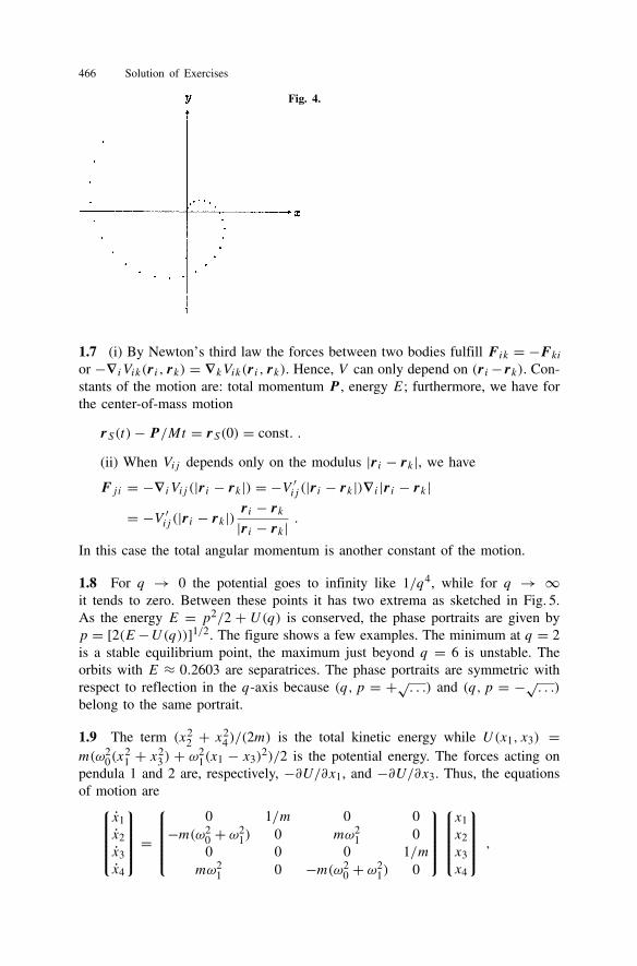
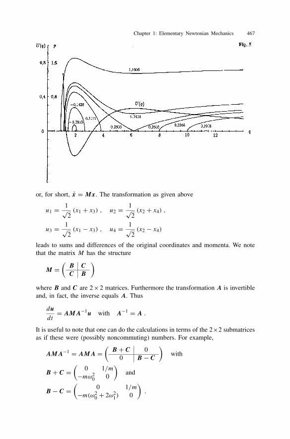
1.8 For q → 0 the potential goes to infinity like 1/q4, while for q → ∞it tends to zero. Between these points it has two extrema as sketched in Fig. 5.As the energy E = p2/2 + U(q) is conserved, the phase portraits are given byp = [2(E−U(q))]1/2. The figure shows a few examples. The minimum at q = 2is a stable equilibrium point, the maximum just beyond q = 6 is unstable. Theorbits with E ≈ 0.2603 are separatrices. The phase portraits are symmetric withrespect to reflection in the q-axis because (q, p = +√. . .) and (q, p = −√. . .)belong to the same portrait.
1.9 The term (x22 + x2
4 )/(2m) is the total kinetic energy while U(x1, x3) =m(ω2
0(x21 + x2
3 ) + ω21(x1 − x3)
2)/2 is the potential energy. The forces acting onpendula 1 and 2 are, respectively, −∂U/∂x1, and −∂U/∂x3. Thus, the equationsof motion are⎧⎪⎪⎪⎪⎪⎪⎪⎪⎪⎩
x1x2x3x4
⎫⎪⎪⎪⎪⎪⎪⎪⎪⎪⎭ =⎧⎪⎪⎪⎪⎪⎪⎪⎪⎪⎩
0 1/m 0 0−m(ω2
0 + ω21) 0 mω2
1 00 0 0 1/mmω2
1 0 −m(ω20 + ω2
1) 0
⎫⎪⎪⎪⎪⎪⎪⎪⎪⎪⎭⎧⎪⎪⎪⎪⎪⎪⎪⎪⎪⎩x1x2x3x4
⎫⎪⎪⎪⎪⎪⎪⎪⎪⎪⎭ ,
Chapter 1: Elementary Newtonian Mechanics 467
or, for short, x =Mx. The transformation as given above
u1 = 1√2(x1 + x3) , u2 = 1√
2(x2 + x4) ,
u3 = 1√2(x1 − x3) , u4 = 1√
2(x2 − x4)
leads to sums and differences of the original coordinates and momenta. We notethat the matrix M has the structure
M =(
B C
C B
)where B and C are 2×2 matrices. Furthermore the transformation A is invertibleand, in fact, the inverse equals A. Thus
du
dt= AMA−1u with A−1 = A .
It is useful to note that one can do the calculations in terms of the 2×2 submatricesas if these were (possibly noncommuting) numbers. For example,
AMA−1 = AMA =(
B + C 00 B − C
)with
B + C =(
0 1/m−mω2
0 0
)and
B − C =(
0 1/m−m(ω2
0 + 2ω21) 0
).
468 Solution of Exercises
This system now separates into two independent oscillators that can be solved inthe usual manner. The first has frequency ω(1) = ω0 (the two pendula performparallel, in-phase oscillations); the second has frequency ω(2) = (ω2
0 + 2ω21)
1/2
(the pendula swing in antiphase). The general solution is
u1 = a1 cos(ω(1)t + ϕ1) , u3 = a2 cos(ω(2)t + ϕ2) .
As an example, consider the initial configuration
x1(0) = a , x2(0) = 0 , x3(0) = 0 , x4(0) = 0 ,
which means that, initially, pendulum 1 is at maximal elongation with vanishingvelocity while pendulum 2 is at rest. The initial configuration is realized by takinga2 = a1 = a
√2, ϕ1 = ϕ2 = 0. This gives
x1(t) = a cosω(1) + ω(2)
2t cos
ω(2) − ω(1)2
t = a cosΩt cosωt ,
x3(t) = a sinω(1) + ω(2)
2t sin
ω(2) − ω(1)2
t = a sinΩt sinωt ,
Where Ω := (ω(1)+ω(2))/2, ω := (ω(2)−ω(1))/2. If Ω/ω = p/q with p, q ∈ Z
and p > q, hence rational, the system returns to its initial configuration after timet = 2πp/Ω = 2πq/ω. For earlier times one has t = πp/(2Ω): x1 = 0, x3 = a(pendulum 1 at rest, pendulum 2 has maximal elongation); t = πp/Ω: x1 = −a,x3 = 0; t = 3πp/(2Ω): x1 = 0, x3 = −a. The oscillation moves back and forthbetween pendulum 1 and pendulum 2. If Ω/ω is not rational, the system will comeclose, at a later time, to the initial configuration but will never assume it exactly(cf. Exercise 6.2). In the example considered here, this will happen if Ωt ≈ 2πnand ωt ≈ 2πm (with m, n ∈ Z), i.e. if Ω/ω can be approximated by the ratio oftwo integers. It may happen that these integers are large so that the “return time”becomes very large.
1.10 As the differential equation is linear, the two terms are solutions preciselywhen µ = ω; a and b are integration constants which are fixed by the initialcondition as follows
x(t) = a cosωt + b sinωt ,
p(t) = −amω sinωt +mbω cosωt .
x(0) = x0 gives a = x0, p(0) = p0 gives b = p0/(mω). The solution withω = 0.8, x0 = 1, p0 = 0 reads x(t) = cos(0.8t).
1.11 From the ansatz one has
x(t) = αx(t)+ eαt (−ωx0 sin ωt + p0/m cos ωt)
x(t) = α2x(t)+ 2αeαt (−ωx0 sin ωt + p0/m cos ωt)
−eαt ω2(x0 cos ωt + p0/mω sin ωt)
= −α2x + 2αx − ω2x .
Chapter 1: Elementary Newtonian Mechanics 469
Inserting and comparing coefficients one finds
α = −κ2, ω =
√ω2 − α2 =
√ω2 − κ2/4 .
The special solution x(t) = e−κt/2 cos(√
0.64− κ2/4 t), approaches the origin ina spiraling motion as t →∞.
1.12 Energy conservation formulated for the two domains yields
m
2v2
1 + U1 = E = m2
v22 + U2 .
As the potential energy U depends on x only there can be no force perpendicularto the x-axis. Therefore, the component of the momentum along the direction per-pendicular to that axis cannot change in going from x < 0 to x > 0: v1⊥ = v2⊥.The law of conservation of energy hence reads
m
2v2
1⊥ +m
2v2
1‖ + U1 = m2
v22⊥ +
m
2v2
2‖ + U2 , or
m
2v2
1‖ + U1 = m2
v22‖ + U2 .
from which follows
sin2 α1 = v21⊥v2
1
, sin2 α2 = v22⊥v2
2
, directly yielding
sin α1
sin α2= |v2||v1| .
For U1 < U2 we find |v1| > |v2|, hence α1 < α2. For U1 < U2 all inequalitiesare reversed.
1.13 Let M = m1 +m2 +m3 be the total mass and m12 = m1 +m2. From thefigure one sees that r2 + sa = r1, s12 + sb = r3, where s12 is the center-of-masscoordinate of particles 1 and 2. Solving for r1, r2, r3 we find
r1 = rS − m3
Msb + m2
m12sa ,
r2 = rS − m3
Msb − m1
m12sa ,
r3 = rS + m12
Msb .
Inserting these into the kinetic energy all mixed terms cancel. The result containsonly terms quadratic in rS, sa, sb
T = 1
2M r2
S︸ ︷︷ ︸TS
+ 1
2µa s
2a︸ ︷︷ ︸
Ta
+ 1
2µb s
2b︸ ︷︷ ︸
Tb
with µa = m1m2
m12, µb = m12m3
M.
470 Solution of Exercises
Fig. 6.
TS is the kinetic energy of the center-of-mass motion, µa is the reduced mass ofthe subsystem consisting of particles 1 and 2. µb is the reduced mass of the sub-system consisting of particle 3 and the center-of-mass S12 of particles 1 and 2, Tbis the kinetic energy of the relative motion of particle 3 and S12.
In an analogous way, the angular momentum is found to be
L =∑i
li = MrS × rS︸ ︷︷ ︸lS
+ µasa × sa︸ ︷︷ ︸la
+ µbsb × sb︸ ︷︷ ︸lb
,
all mixed terms having cancelled.By a special (and proper) Galilei transformation, rS → r ′s = rS + wt + a,
rS → r ′S = rS + w, sa → sa , sb → sb and, hence,
l′S = lS +M(a × (rS + w)+ (rS − t rS)× w) ,
while l′a = la , l′b = lb remain unchanged.
1.14 (i) With U(λr) = λαU(r) and r ′ = λr the forces from U (r ′) := U(λr) andfrom U(r), respectively, differ by the factor λα−1. Indeed
F ′ = −∇r ′U = −1
λ∇r U = −λα−1∇rU = λα−1F .
Integrating F ′ · dr ′ over a path in r ′ space and comparing with the correspond-ing integral over F · dr , the work done in the two cases differs by the factor λα .Changing t to t ′ = λ1−α/2t ,(
dr ′
dt ′
)2
= λ2λα−2(dr
dt
)2
,
which means that the kinetic energy
T = 1
2m
(dr ′
dt ′
)2
Chapter 1: Elementary Newtonian Mechanics 471
differs from the original one by the same factor λα . Thus, this holds for the totalenergy, too, E′ = λαE. The indicated relation between time differences and lineardimensions of geometrically similar orbits follows.
(ii) For harmonic oscillation the assumption holds with α = 2. The ratio ofthe periods of two geometrically similar orbits is Ta/Tb = 1, independently of thelinear dimensions.
In the homogeneous gravitational field U(z) = mgz and, hence, α = 1. Timesof free fall and initial height H are related by T ∝ H 1/2.
In the case of the Kepler problem U = −A/r and, hence, α = −1. Two geo-metrically similar ellipses with semimajor axes aa and bb have circumference Uaand Ub, respectivley, such that Ua/Ub = aa/ab. Therefore the ratio of the peri-ods Ta and Tb is Ta/Tb = (Ua/Ub)3/2 from which follows (Ta/Tb)2 = (aa/ab)3,Kepler’s third law.
(iii) The general relation is Ea/Eb = (La/Lb)α . If Ai denotes the ampli-
tude of harmonic oscillation, Ea/Eb = A2a/A
2b. In the case of Kepler motion
Ea/Eb = ab/aa : the energy is inversely proportional to the semimajor axis.
1.15 (i) From the equations of Sect. M1.24
rP = p
1+ ε = −A
2E
1− ε2
1+ ε = −A
2E(1− ε) ;
rA = − A2E(1+ ε) .
From these we calculate
rP + rA = −AE, rP · rA = A2
4E2(1− ε2) = l2
−2µE.
Inserting this into the differential equation we obtain
dφ
dr= l
r2
√2µ
(E + A
r− l2
2µr2
) .
This is precisely eq. (M1.67) with Ueff = −A/r+ l2/2µr2. Integration of eq. (1.4)with the boundary condition as indicated implies
φ(r)− φ(rP ) =∫ r
rP
1
r
(rP rA
(r − rP )(rA − r))1/2
dr .
We make use of the indicated formula with
α = 2rArP
rA − rP , β = − rA + rPrA − rP ,
and obtain
472 Solution of Exercises
φ(r) = arccos2rArP − (rA + rP )r
(rA − rP )r .
(ii) There are two possibilities for solving this equation: (a) the new equationsare obtained by replacing l2 with l2 = l2 + 2µB. For the remainder, the solutionis exactly the same as for the Kepler problem. If B > 0(B < 0), then l > l(l < l),i.e., in the case of repulsion (attraction) the orbit becomes larger (smaller). (b)With U(r) = U0(r)+ B/r2, U0(r) = −A/r , the differential equation for φ(r) iswritten in the same form as above
dφ
dr=
√rArP
r
√(r − r ′P)(r ′A − r)
,
where r ′P, r ′A denote perihelion and aphelion, respectively, for the perturbed poten-tial. They are obtained from the formula (r−rP)(rA−r)+B/E = (r−r ′P)(r ′A−r).Multiplying the differential equation by ((r ′Pr ′A)/(rPrA))1/2 and integrating as be-fore
φ(r) =√rPrA
r ′Pr ′Aarccos
2r ′Ar ′P − r(r ′A + r ′P)r(r ′A − r ′P)
.
From this solution follows r(φ) = 2r ′Pr ′A/[r ′P+ r ′A+ (r ′A− r ′P) cos√r ′Pr ′A/rPrA φ].
The first passage through perhelion is set to φP1 = 0. The second is φP2 =2π((rPrA)/(r ′Pr ′A))1/2 = 2πl/
√l2 + 2µB ≈ 2π(1 − µB/l2). The perhelion pre-
cession is (φP2 − 2π). It is independent of the energy E. For B > 0 (additionalrepulsion) the motion lags behind, and for B < 0 (additional attraction) the motionadvances as compared to the Kepler case.
1.16 For fixed l, the energy must fulfill E ≥ −µA2/(2l2). The lower limit is as-sumed for circular orbits with radius r0 = l2/µA. The semimajor axis (in relativemotion) follows from Kepler’s third law a3 = GN(mE+mS)T
2/(4π2). This givesa = 1.495× 10¹¹ m (T = 1 y = 3.1536× 10⁷ s). This is approximately equal toaE, the semimajor axis of the earth in the center-of-mass system. The sun moveson an ellipse with semimajor axis
aS = mE
mE +mSa ≈ 449 km .
This is far within the sun’s radius RS ≈ 7× 10⁵ km.
1.17 We arrange the two dipoles as sketched in Fig. 7. The potential created bythe first dipole at a point situated at r is
Φ1 = e1
(1
|r − d1| −1
|r|)≈ e1
(1
r+ r · d1
r3− 1
r
)= r · (e1d1)
r3.
Chapter 1: Elementary Newtonian Mechanics 473
Fig. 7.
Here, we have expanded
1
|r − d1| =1√
r2 + d21 − 2r · d1
up to the term linear in d1. In the limit we obtain Φ1 = r · p1/r3. The potential
energy of the second dipole in the field of the first reads
W = e1(Φ1(r + d2)−Φ1(r)) = e2
(p1 · (r + d2)
|r + d2|3 − p1 · rr3
).
Expanding again up to terms linear in d2
W ≈ e2
(p1 · rr3
(1− 3
r · d2
r2
)+ p1 · d2
r3− p1 · r
r3
).
Finally, taking the limit e2 →∞, d2 → 0, with e2d2 = p2 finite, this yields
W(1, 2) = p1 · p2
r3− 3(p1 · r)(p2r)
r5.
From this expression one calculates the components of F 21 = −∇1W = −F 12,making use of relations such as
∂
∂x1= ∂r
∂x1
∂
∂r= x1 − x2
r
∂
∂r, etc. .
So, for example∂W(1, 2)
∂x1= −(p1 · p2)
3
r4
x1 − x2
r− 3
r5
(px1 (p2 · r)
+(p1 · r)px2)+ (p1 · r)(p2 · r)
15
r6
x1 − x2
r.
1.18 Take the time derivative of r · a,
d
dtr · a = r · a = v · a = (v × a) · a = 0 .
Thus, r ·a is constant in time and the indicated relation holds for all times. Takingthe time derivative of (5) and inserting v, we find v = v × a = (v × a) × a =
474 Solution of Exercises
−a2v+(v ·a)a. The second term is constant as shown above. Thus, integrating thisequation over t from 0 to t , we have r(t)− r(0) = −ω2(r(t)−r(0))+(v(0) ·a)at ,where ω2 := a2. By eq. (5) r(0) = v(0)× a, so that we may write
r(t)+ ω2r(t) = (v(0) · a)at + v(0)× a + ω2r(0) .
This is the desired form, the general solution of the homogeneous differential equa-tions is
rhom(t) = c1 sinωt + c2 cosωt .
With the given ansatz for a special solution of the inhomogeneous equation theconstants are found to be
c1 = 1
ω3
(a2v(0)− (v(0) · a)a
)= 1
ω3(a × (v(0)× a))
c2 = − 1
ω2v(0)× a
c = 1
ω2(v(0) · a)a
d = 1
ω2v(0)× a + r(0) .
The solution therefore reads
r(t) = 1
ω3a × (v(0)× a) sinωt + 1
ω2(v(0) · a)at
+ 1
ω2v(0)× a(1− cosωt)+ r(0) .
It represents a helix winding around the vector a.
1.19 The ball falls from initial height h0. It hits the plane for the first time att1 = √2h0/g, the velocity then being u1 = −√2h0g = −gt1. Furthermore, withα := √(n− 1)/n
vi = −αui , ui+1 = −vi , ti+1 − ti = 2vig.
The first two equations give v1 = αgt1 and vi = αigt1. The third equation yields
t0i − ti =vi
g= ti+1 − t0i and t0i+1 − ti+1 = vi+1
g,
and, from there, t0i+1 − t0i = (vi+1 + vi)/g = t1(α + 1)αi . With t00 = 0 we haveat once
t0i = t1(1+ α)i−1∑ν=0
αv .
From hi = v2i /(2g), finally, hi = α2ih0.
Chapter 1: Elementary Newtonian Mechanics 475
1.20 The answer is contained in the following table giving the products of theelements
E P T P · TE E P T P · TP P E P · T T
T T P · T E P
P · T P · T T P E
1.21 Let R and E0 denote the radius and the energy of a circular orbit, respec-tively. The differential equation for the radial motion reads
dr
dt=
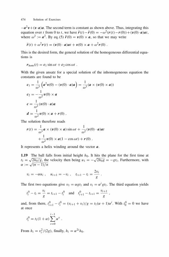
√2
µ
√E0 − Ueff(r) , Ueff(r) = U(r)+ l2
2µr2.
From this follows E0 = Ueff(R), U ′eff
∣∣r=R = 0, U ′′eff
∣∣r=R > 0 or, for U(r),
U ′(R) = l2
µ
1
R3and U ′′(R) > −3l2
µ
1
R4.
If E = E0 + ε,dr
dt=
√2
µ
√ε − 1
2(r − R)2U ′′eff(R) .
Setting κ := U ′′eff(R) we obtain, choosing ς = r ′ − R,
t − t0 =√µ
κ
∫ r−R
r0−Rdς√
2ε/κ − ς2=
õ
κarcsin
((r − R)
√κ
2ε
).
Solving for r − R yields
r − R =√
2ε
κsin
√κ
µ(t − t0) .
Thus, the radial distance oscillates around the value R. More specifically, one finds(i) U(r) = rn, U ′(r) = nrn−1, U ′′(r) = n(n−1)rn−2. This yields the equation
nRn−1 = l2
µR3⇒ R = n+2
√l2
µn,
κ = n(n− 1)Rn−2 + 3l2
µR4> 0 ⇔ n(n− 1)Rn+2︸ ︷︷ ︸
l2/(µn)
+ 3l2
µ= (n+ 2)l2
µ> 0 .
(ii) U(r) = λ/r , U ′(r) = −λ/r2, U ′′(r) = 2λ/r3. From this R = −l2/(µλ),κ = −λ/R3. This is greater than zero of λ is negative.
476 Solution of Exercises
1.22 (i) The eastward deviation follows from the formula given in Sect. M1.26,∆ ≈ (2√2 /3)g−1/2H 3/2ω cosϕ. With ω = 2π/(1 day) = 7.27 × 10⁻⁵ s−1 andg = 9.81 ms−2 one finds ∆ ≈ 2.2 cm.
(ii) We proceed as in Sect. M1.26 (b) and determine the eastward deviation ufrom the linearized ansatz r(t) = r(0)(t)+ ωu(t), inserting here the unperturbedsolution, r0(t) = gt (T − 1
2 t)ev . This gives (d ′2/dt2)u(t) ≈ 2g cosϕ(t − T )ev .Integrating twice,
u(t) = 1
3g cosϕ(t3 − 3T t2)e0 .
The stone returns to the surface of the earth after time t = 2T . The eastward de-viation is found to be negative, ∆ ≈ − 4
3gω cosϕT 3, which means, in reality, thatit is a westward deviation. Its magnitude is four times larger than in case (i).
(iii) Denote the eastward deviation by u as before (directed from west to east),the southward deviation by s (directed from north to south). A local, earth-bound,coordinate system is given by (e1, e0, ev), e1 defining the direction N–S, e0 andev being defined as in Sect. M1.26 (b). Thus, u = ue0, s = se1. The equation ofmotion (M1.74′), together with ω = ω(− cosϕ, 0, sin ϕ), implies
s = 2ω2 sin ϕu .
Inserting the approximate solution u ≈ 13gt
3 cosϕ and integrating over time twice,one obtains
s(t) = 1
6ω2g sin ϕ cosϕt4 .
1.23 For E > 0 all orbits are scattering orbits. If l2 > 2µα,
φ − φ0 = l√2µE
∫ r
r0
dr ′√r ′2 − (l2 − 2µα)/(2µE)
= r(0)p∫ r
r0
dr ′
r ′√r ′2 − r2
P
, (1)
where µ is the reduced mass, rP = √(l2 − 2µα)/(2µE) the perihelion and
r(0)P = l/√2µE. The particle is assumed to come from infinity, traveling parallel
to the x-axis. Then the solution is φ(r) = l/√l2 − 2µα arcsin(rP/r). If α = 0,the corresponding solution is φ(0)(r) = arcsin(r(0)P /r); the particle moves along a
straight line parallel to the x-axis, at the distance r(0)P . For α = 0
φ(r = rP) = l√l2 − 2µα
π
2,
that is, after the scattering and asymptotically, the particle moves in the directionl/√l2 − 2µα π . Before that it travels around the center of force n times if the
condition
Chapter 1: Elementary Newtonian Mechanics 477
l√l2 − 2µα
(arcsin
rP
∞ − arcsinrP
rP
)= r
(0)P
rP
(π − π
2
)> nπ
is fulfilled. The number
n =[r(0)P
2rP
]is independent of energy E.
In the case l2 < 2µα eq. (1) can also be integrated. With the same initial con-dition one obtains
φ(r) = r(0)P
blnb +√b2 + r2
r,
where b = ((2µα − l2)/(2µE))1/2. The particle travels around the force centeron a spiral-like orbit, towards the center. As the radial distance tends to zero, theangular velocity increases in such a way as to respect Kepler’s second law (M1.22).
1.24 Let the comet and the sun approach each other with energy E. Long be-fore the collision the relative momentum has the magnitude q = √2µE, with µthe reduced mass, the angular momentum has the magnitude l = qb. The cometcrashes when the perihelion rP of its hyperbola is smaller or equal R, i.e., whenb ≤ bmax with bmax following from the condition rP = R, viz.
p
1+ ε = R with pl2
Aµ= q
2b2
Aµ, ε =
√1+ 2Eq2b2
µA2
and A = GmM . One finds bmax = √1+ A/(ER) and, hence,
σ =∫ bmax
02πb db = πR2
(1+ A
ER
).
For A = 0 this is the area of the sun seen by the comet. With increasing gravi-tational attraction (A > 0) this surface increases by the ratio (potential energy atthe sun’s edge)/(energy of relative motion).
1.25 As explained in Sect. M1.21.2 the equation of motion reads
x = Ax + b ,
with A as given in eq. (M1.50), and
A =
⎧⎪⎪⎪⎪⎪⎪⎪⎪⎪⎪⎪⎪⎪⎪⎪⎪⎪⎩
0 0 0 1/m 0 00 0 0 0 1/m 00 0 0 0 0 1/m0 0 0 0 K 00 0 0 −K 0 00 0 0 0 0 0
⎫⎪⎪⎪⎪⎪⎪⎪⎪⎪⎪⎪⎪⎪⎪⎪⎪⎪⎭, b = e
⎧⎪⎪⎪⎪⎪⎪⎪⎪⎪⎪⎪⎪⎪⎪⎪⎪⎪⎩
000ExEyEz
⎫⎪⎪⎪⎪⎪⎪⎪⎪⎪⎪⎪⎪⎪⎪⎪⎪⎪⎭.
478 Solution of Exercises
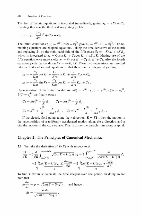
The last of the six equations is integrated immediately, giving x6 = eEt + C1.Inserting this into the third and integrating yields
x3 = z = eEz2m
t2 + C1t + C2 .
The initial conditions z(0) = z(0), z(0) = v(0)z give C2 = z(0), C1 = v(0)z . The re-maining equations are coupled equations. Taking the time derivative of the fourthand replacing x5 by the right-hand side of the fifth gives x4 = −K2x4 + eKEywhich is integrated to x4 = C3 sinKt + C4 cosKt + eEy/K . Making use of thefifth equation once more yields x3 = C3 cosKt −C4 sinKt +C5. Also the fourthequation yields the condition C5 = −eEx/K . These two expressions are insertedinto the first and second equations so that these can be integrated yielding
x1 = − C3
KmcosKt + C4
KmsinKt + e
KmEyt + C6
x2 = + C3
KmsinKt + C4
KmcosKt − e
KmExt + C7 .
Upon insertion of the initial conditions x(0) = x(0), y(0) = y(0), x(0) = v(0)x ,y(0) = v(0)y we finally obtain
C3 = mv(0)y + e
KEx , C4 = mv(0)x − e
KEy ,
C6 = x(0) + v(0)y
K+ e
mK2Ex , C7 = y(0) − v
(0)x
K+ e
mK2Ey .
If the electric field points along the z-direction, E = Eez, then the motion isthe superposition of a uniformly accelerated motion along the z-direction and acircular motion in the (x, y)-plane. That is to say the particle runs along a spiral.
Chapter 2: The Principles of Canonical Mechanics
2.1 We take the derivative of F(E) with respect to E
dF
dE= 2
d
dE
∫ qmax(E)
qmin(E)
√2m(E − U(q)) dq = 2
∫ qmax(E)
qmin(E)
m√2m(E − U(q)) dq
+2√
2m(E − U(qmax))︸ ︷︷ ︸=0
dqmax
dE− 2
√2m(E − U(qmin))︸ ︷︷ ︸
=0
dqmin
dE.
To find T we must calculate the time integral over one period. In doing so wenote that
mdq
dt= p = √
2m(E − U(q)) , and hence ,
dt = mdq√2m(E − U(q)) .
Chapter 2: The Principles of Canonical Mechanics 479
Therefore,
T = 2∫ qmax(E)
qmin(E)
m√2m(E − U(q)) dq .
This, however, is precisely the expression calculated above. For the example ofthe oscillator with q = q0 sinωt , p = mωq0 cosωt , one finds F = mωπq2
0 =(2π/ω)E and T = 2π/ω.
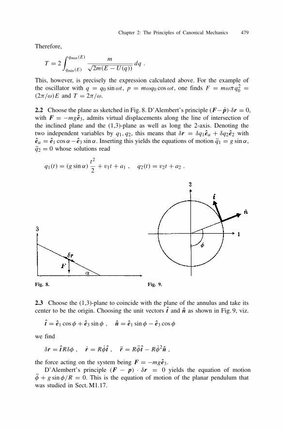
2.2 Choose the plane as sketched in Fig. 8. D’Alembert’s principle (F−p)·δr = 0,with F = −mge3, admits virtual displacements along the line of intersection ofthe inclined plane and the (1,3)-plane as well as long the 2-axis. Denoting thetwo independent variables by q1, q2, this means that δr = δq1eα + δq2e2 witheα = e1 cosα− e3 sin α. Inserting this yields the equations of motion q1 = g sin α,q2 = 0 whose solutions read
q1(t) = (g sin α)t2
2+ v1t + a1 , q2(t) = v2t + a2 .
Fig. 8. Fig. 9.
2.3 Choose the (1,3)-plane to coincide with the plane of the annulus and take itscenter to be the origin. Choosing the unit vectors t and n as shown in Fig. 9, viz.
t = e1 cosφ + e3 sin φ , n = e1 sin φ − e3 cosφ
we find
δr = tRδφ , r = Rφ t , r = Rφ t − Rφ2n ,
the force acting on the system being F = −mge3.D’Alembert’s principle (F − p) · δr = 0 yields the equation of motion
φ + g sin φ/R = 0. This is the equation of motion of the planar pendulum thatwas studied in Sect. M1.17.
480 Solution of Exercises
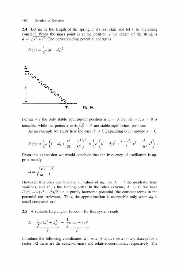
2.4 Let d0 be the length of the spring in its rest state and let κ be the stringconstant. When the mass point is at the position x the length of the string isd = √x2 + l2. The corresponding potential energy is
U(x) = 1
2κ(d − d0)
2 .
Fig. 10.
For d0 ≤ l the only stable equilibrium position is x = 0. For d0 > l, x = 0 is
unstable, while the points x = ±√d2
0 − l2 are stable equilibrium positions.As an example we study here the case d0 ≤ l. Expanding U(x) around x = 0,
U(x) ≈ 1
2κ
(l − d0 + x
2
2l− x4
8l3
)2
≈ 1
2κ
((l − d0)
2 + l − d0
lx2 + d0
4l3x4).
From this expression we would conclude that the frequency of oscillation is ap-proximately
ω =√κ
m
l − d0
l.
However, this does not hold for all values of d0. For d0 = l the quadratic termvanishes, and x4 is the leading order. In the other extreme, d0 = 0, we haveU(x) = κ(x2 + l2)/2, i.e. a purely harmonic potential (the constant terms in thepotential are irrelevant). Thus, the approximation is acceptable only when d0 issmall compared to l.
2.5 A suitable Lagrangian function for this system reads
L = 1
2m(x2
1 + x22 )︸ ︷︷ ︸
T
− 1
2κ(x1 − x2)
2︸ ︷︷ ︸U
.
Introduce the following coordinates: u1 := x1 + x2, u2 := x1 − x2. Except for afactor 1/2 these are the center-of-mass and relative coordinates, respectively. The
Chapter 2: The Principles of Canonical Mechanics 481
Lagrangian becomes L = m(u21 + u2
2)/4 − κu22/2. The equations of motion that
follow from it are
u1 = 0 , mu2 + 2κu2 = 0 .
The solutions are u1 = C1t +C2, u2 = C3 sinωt +C4 cosωt , with ω = √2κ/m.It is not difficult to rewrite the initial conditions in the new coordinates, viz.
u1(0) = +l u1(0) = v0
u2(0) = −l u2(0) = v0 .
The constants are determined from these so that the final solution is
x1(t) = v0
2
(t + 1
ωsinωt
)− l
2(1− cosωt)
x2(t) = v0
2
(t − 1
ωsinωt
)+ l
2(1+ cosωt) .
2.6 By hypothesis F(λx1, . . . , λxn) = λNF(x1, . . . , xN). We take the firstderivative of this equation with respect to λ and set λ = 1. The left-hand side is
d
dλF(λx1, . . . , λxn)
∣∣∣∣λ=1
=n∑i=1
∂F
∂xi
d(λxi)
dλ
∣∣∣∣λ=1
=n∑i=1
∂F
∂xixi .
The same operation on the right-hand side gives NF .
2.7 In the general case the Euler-Lagrange equation reads
∂f
∂y= d
dx
∂f
∂y′.
Multiply this equation by y′ and add the term y′′∂f/∂y′ on both sides. The right-hand side is combined to
y′ ∂f∂y+ y′′ ∂f
∂y′= d
dx
(y′ ∂f∂y′
).
If f does not depend explicitly on x then the left-hand side is df (y, y′)/dx. Thewhole equation can be integrated directly and yields the desired relation. Applyingthis result to L(q, q) = T (q)− U(q) gives∑
i
qi∂T (q)
∂qi− T + U = const. .
If T is a homogeneous, quadratic form in q the solution to Exercise 2.6 tells usthat the first term equals 2T . Therefore, the constant is the energy E = T + U .
482 Solution of Exercises
2.8 (i) We must minimize the arc length
L =∫ds =
∫ x2
x1
√1+ y′2 dx
i.e. we must choose f (y, y′) = √1+ y′2. Applying the result of the preceding
exercise we obtain
y′√y′√
1+ y′2 −√
1+ y′2 = const. ,
or y′ = const. Thus, y = ax + b. Inserting the boundary conditions y(x1) = y1,y(x2) = y2 gives
y(x) = y2 − y1
x2 − x1(x − x1)+ y1 .
(ii) The position of the center of mass is determined by the equation
MrS =∫r dm ,
M denoting the mass of the chain, dm the mass element. If λ is the mass per unitlength, dm = λ ds. As the x-coordinate of the center of mass is irrelevant, theproblem is to find the shape for which its y-coordinate is lowest. Thus we haveto minimize the functional∫
y ds =∫ x2
x1
y
√1+ y′2 dx .
The result of the preceding exercise leads to
yy′2√1+ y′2 − y
√1+ y′2 = −
√y√
1+ y′2 = C .
This equation can be solved for y′,
y′ =√Cy2 − 1 .
This is a separable differential equation whose general solution is
y(x) = 1√C
cosh(√C x + C′
).
The constants C and C′, finally, must be chosen such that the boundary conditionsy(x1) = y1, y(x2) = x2 are fulfilled.
Chapter 2: The Principles of Canonical Mechanics 483
2.9 (i) In either case the equations of motion read
x1 = −mω20x1 − 1
2m(ω2
1 − ω20)(x1 − x2)
x2 = −mω20x2 + 1
2m(ω2
1 − ω20)(x1 − x2) .
The reason for this result becomes clear when we calculate the difference L′ −L:
L′ − L = −iω0m(x1x1 + x2x2) = − i2ω0m
d
dt(x2
1 + x22 ) .
The two Lagrangian functions differ by the total time derivative of a function whichdepends on the coordinates only. By the general considerations of Sects. M2.9 andM2.10 such an addition does not alter the equations of motion.
(ii) The transformation to eigenmodes reads
z1 = 1√2(x1 + x2) , z2 = 1√
2(x1 − x2) .
This transformation(x1
x2
)−→F
(z1
z2
)is one-to-one. Both F and F−1 are differentiable. Thus, F , being a diffeomor-phism, leaves the Lagrange equations invariant.
2.10 The axial symmetry of the force suggests the use of cylindrical coordinates.In these coordinates the force must not have a component along the unit vectoreφ . Furthermore, since
∇U(r, ϕ, z) = ∂U∂r
er + 1
r
∂U
∂ϕeϕ + ∂U
∂zez ,
U must not depend on ϕ. The unit vectors er and ez span a plane that containsthe z-axis.
2.11 By a (passive) infinitesimal rotation we have
x ≈ x0 − (ϕ × x0) ε or x0 ≈ x + (ϕ × x) ε .
Here ϕ is the direction about which the rotation takes place, ε is the angle of rota-tion, so that ϕε = ω dt . Thus x0 = x+(ω×x), the dot denoting the time derivativein the system of reference that one considers. Inserting this into the kinetic energyone finds
T = m(x2 + 2x · (ω × x)+ (ω × x)2
)/2 .
484 Solution of Exercises
Meanwhile U(x0) becomes U(x) = U (R−1(t)x). We calculate
∂L
∂xi= mxi +m(ω × x)i
∂L
∂xi= −∂U
∂xi+m(x × ω)i +m((ω × x)× ω)i .
This leads to the equation of motion
mx = −∇U − 2m(ω × x)−mω × (ω × x)−m(ω × x) .
2.12 Let the coordinates of the point of suspension be (xA, 0), ϕ the angle be-tween the pendulum and the vertical, with −π ≤ ϕ ≤ π . The coordinates of themass point are
x = xA + l sin ϕ , y = −l cosϕ ,
m denoting the mass, l the length of the pendulum. Inserting these into
L = m2(x2 + y2)−mg(y + l)
gives the answer
L = m2(x2A + l2ϕ2 + 2l cosϕxAϕ)+mgl(cosϕ − 1) .
2.13 (i) If the oscillation is to be harmonic s(t) must obey the following equation
s + κ2s = 0 ⇒ s(t) = s0 sin κt .
(ii) The Lagrangian function reads
L = m2s2 − U
where the potential energy is given by (see Fig. 11)
U = mgy = mg∫ s
0sin φ ds .
The Euler-Lagrange equation reads ms+mg sin φ = 0. Inserting the above relationfor s(t) we obtain the equation s0κ2 sin κt = g sin φ.
Fig. 11.
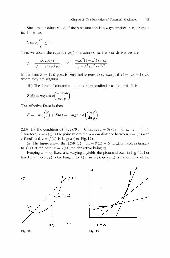
Chapter 2: The Principles of Canonical Mechanics 485
Since the absolute value of the sine function is always smaller than, or equalto, 1 one has
λ := s0 κ2
g≤ 1 .
Thus we obtain the equation φ(t) = arcsin(λ sin κt) whose derivatives are
φ = λκ cos κt√1− λ2 sin2 κt
, φ = −λκ2(1− λ2) sin κt
(1− λ2 sin2 κt)3/2.
In the limit λ→ 1, φ goes to zero and φ goes to κ , except if κt = (2n+ 1)/2πwhere they are singular.
(iii) The force of constraint is the one perpendicular to the orbit. It is
Z(φ) = mg cosφ
(− sin φ
cosφ
).
The effective force is then
E = −mg(
0
1
)+ Z(φ) = −mg sin φ
(cosφ
sin φ
).
2.14 (i) The condition ∂F (x, z)/∂x = 0 implies z− ∂f/∂z = 0, i.e., z = f ′(x).Therefore, x = x(z) is the point where the vertical distance between y = zx (withz fixed) and y = f (x) is largest (see Fig. 12).
(ii) The figure shows that (LΦ)(z) = zx−Φ(z) ≡ G(x, z), z fixed, is tangentto f (x) at the point x = x(z) (the derivative being z).
Keeping x = x0 fixed and varying z yields the picture shown in Fig. 13. Forfixed z y = G(x, z) is the tangent to f (x) in x(z). G(x0, z) is the ordinate of the
Fig. 12. Fig. 13.
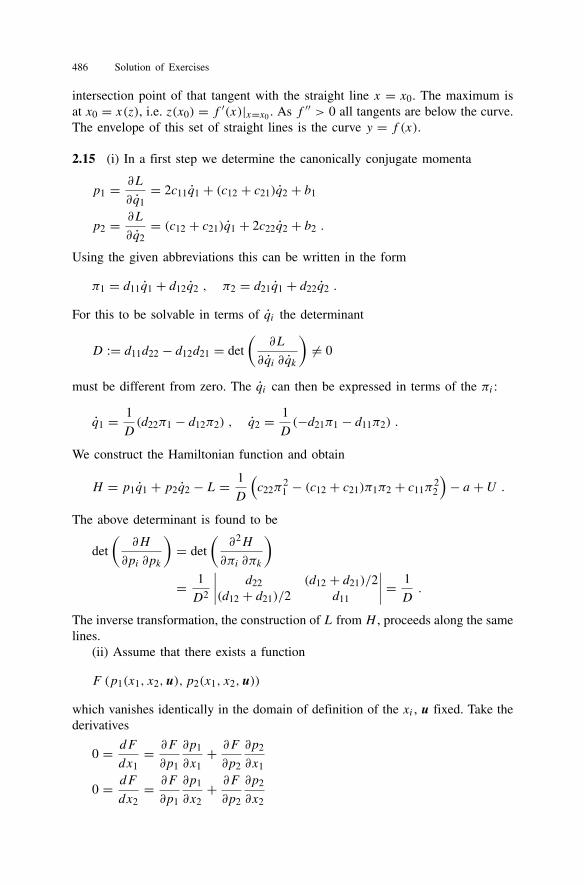
486 Solution of Exercises
intersection point of that tangent with the straight line x = x0. The maximum isat x0 = x(z), i.e. z(x0) = f ′(x)|x=x0 . As f ′′ > 0 all tangents are below the curve.The envelope of this set of straight lines is the curve y = f (x).
2.15 (i) In a first step we determine the canonically conjugate momenta
p1 = ∂L
∂q1= 2c11q1 + (c12 + c21)q2 + b1
p2 = ∂L
∂q2= (c12 + c21)q1 + 2c22q2 + b2 .
Using the given abbreviations this can be written in the form
π1 = d11q1 + d12q2 , π2 = d21q1 + d22q2 .
For this to be solvable in terms of qi the determinant
D := d11d22 − d12d21 = det
(∂L
∂qi ∂qk
)= 0
must be different from zero. The qi can then be expressed in terms of the πi :
q1 = 1
D(d22π1 − d12π2) , q2 = 1
D(−d21π1 − d11π2) .
We construct the Hamiltonian function and obtain
H = p1q1 + p2q2 − L = 1
D
(c22π
21 − (c12 + c21)π1π2 + c11π
22
)− a + U .
The above determinant is found to be
det
(∂H
∂pi ∂pk
)= det
(∂2H
∂πi ∂πk
)= 1
D2
∣∣∣∣ d22 (d12 + d21)/2(d12 + d21)/2 d11
∣∣∣∣ = 1
D.
The inverse transformation, the construction of L from H , proceeds along the samelines.
(ii) Assume that there exists a function
F (p1(x1, x2,u), p2(x1, x2,u))
which vanishes identically in the domain of definition of the xi , u fixed. Take thederivatives
0 = dF
dx1= ∂F
∂p1
∂p1
∂x1+ ∂F∂p2
∂p2
∂x1
0 = dF
dx2= ∂F
∂p1
∂p1
∂x2+ ∂F∂p2
∂p2
∂x2
Chapter 2: The Principles of Canonical Mechanics 487
By assumption the partial derivatives of F with respect to pi do not vanish (oth-erwise the system of equations would be trivial). Therefore, the determinant
D = det
⎧⎪⎪⎪⎪⎪⎪⎪⎪⎪⎪⎩∂p1
∂x1
∂p2
∂x1∂p1
∂x2
∂p2
∂x2
⎫⎪⎪⎪⎪⎪⎪⎪⎪⎪⎪⎭ = det
(∂2L
∂xi ∂xk
)
must be different from zero. This proves the assertion.
2.16 We introduce the complex variable w := x + iy. Then
x = (w + w∗)/2 , y = −i(w − w∗)/2 , x2 + y2 = ww∗ .l3 is calculated to be
l3 = m(xy − yx) = m2i(ww∗ − ww∗) .
Expressed in the new coordinates the Lagrangian function reads
L = m2(ww∗ + z2)− imω
4(ww∗ − ww∗) .
The equations of motion are
m
2w∗ − imω
4w∗ = imω
4w∗ , mz = 0 .
The first of these is written in terms of the variable u := w∗. It becomes u = iωu,its solution being u = eiωt . w∗ is the time integral of this function, viz.
w∗ = − i
ωeiωt + C ,
where C is a complex constant. Take the complex conjugate
w = i
ωe−iωt + C∗ ,
from which follow the solutions for x and y
x = 1
ωsinωt + C1 , y = 1
ωcosωt + C2 ,
where C1 = (C, C2 = −)C.The solution for the z coordinate is simple: z = C3t+C4, i.e., uniform motion
along a straight line. The canonically conjugate momenta are
px = mx − m2ωy , py = my + m
2ωx , pz = mz ,
488 Solution of Exercises
while the kinetic momenta are given by pkin = mx. In order to construct the Hamil-tonian function the velocities are expressed in terms of the canonical momenta
x = 1
mpx + ω
2y , y = 1
mpy − ω
2x , z = 1
mpz .
Then H is found to be
H = p · x − L = 1
2mp2
kin .
2.17 (i) Hamilton’s variational principle, when applied to L, requires
I :=∫ τ2
τ1
L dτ
to be an extremum. Now, since∫ τ2
τ1
L dτ =∫ t2
t1
Ldt with ti = t (τi) , i = 1, 2 ,
the action integral I is extremal if and only if the Lagrange equations that followfrom L are fulfilled.
(ii) We define q = (q1, . . . , qf ), t = qf+1. From Noether’s theorem the quan-tity
I =f+1∑i=1
∂L
∂qi
d
dshs(q1, . . . , qf+1)|s=0
is an integral of the motion provided L is invariant under (q1, . . . , qf+1)
→ hs(q1, . . . , qf+1), i.e., in the case considered here, under (q1, . . . , qf+1) →(q1, . . . , qf+1 + s). Here
dhs
ds
∣∣∣∣s=0
= (0, . . . , 0, 1)
and
∂L
∂qf+1= ∂L
∂(dt/dτ)= L+
f∑i=1
∂L
∂qi
(− 1
(dt/dτ)2
)dqi
dτ
dt
dτ= L−
f∑i=1
∂L
∂qi
dqi
dt.
The integral of the motion is
I = L−f∑i=1
∂L
∂qi
dqi
dt.
Except for a sign this is the expression for the energy.
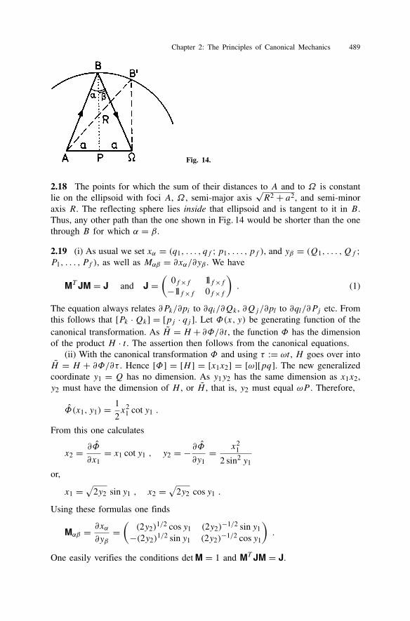
Chapter 2: The Principles of Canonical Mechanics 489
Fig. 14.
2.18 The points for which the sum of their distances to A and to Ω is constantlie on the ellipsoid with foci A, Ω , semi-major axis
√R2 + a2, and semi-minor
axis R. The reflecting sphere lies inside that ellipsoid and is tangent to it in B.Thus, any other path than the one shown in Fig. 14 would be shorter than the onethrough B for which α = β.
2.19 (i) As usual we set xα = (q1, . . . , qf ;p1, . . . , pf ), and yβ = (Q1, . . . ,Qf ;P1, . . . , Pf ), as well as Mαβ = ∂xα/∂yβ . We have
MT JM = J and J =(
0f×f 1lf×f−1lf×f 0f×f
). (1)
The equation always relates ∂Pk/∂pi to ∂qi/∂Qk , ∂Qj/∂pl to ∂ql/∂Pj etc. Fromthis follows that [Pk ·Qk] = [pj · qj ]. Let Φ(x, y) be generating function of thecanonical transformation. As H = H + ∂Φ/∂t , the function Φ has the dimensionof the product H · t . The assertion then follows from the canonical equations.
(ii) With the canonical transformation Φ and using τ := ωt , H goes over intoH = H + ∂Φ/∂τ . Hence [Φ] = [H ] = [x1x2] = [ω][pq]. The new generalizedcoordinate y1 = Q has no dimension. As y1y2 has the same dimension as x1x2,y2 must have the dimension of H , or H , that is, y2 must equal ωP . Therefore,
Φ(x1, y1) = 1
2x2
1 cot y1 .
From this one calculates
x2 = ∂Φ
∂x1= x1 cot y1 , y2 = − ∂Φ
∂y1= x2
1
2 sin2 y1
or,
x1 =√
2y2 sin y1 , x2 =√
2y2 cos y1 .
Using these formulas one finds
Mαβ = ∂xα∂yβ
=((2y2)
1/2 cos y1 (2y2)−1/2 sin y1
−(2y2)1/2 sin y1 (2y2)
−1/2 cos y1
).
One easily verifies the conditions det M = 1 and MT JM = J.
490 Solution of Exercises
2.20 (i) For f = 1 the condition det M = 1 is necessary and sufficient because,quite generally,
MT JM =(
0 1−1 0
)(a11a22 − a12a21) = J det M .
(ii) We calculate S ·O, set it equal to M, and obtain the equations
x cosα − y sin α = a11 (1)
x sin α + y cosα = a12 (2)
y cosα − z sin α = a21 (3)
y sin α + z cosα = a22 (4)
From the combination ((2)− (3))/((1)+ (4)) of the equations
tan α = a12 − a21
a11 + a22.
This allows us to calculate sin α and cosα, so that the subsystems ((1), (2)) and((3), (4)) can be solved for x, y, and z. One finds x = a11 cosα + a12 sin α,z = a22 cosα − a21 sin α, y2 = xz− 1.
There is a special case, however, that must be studied separately: This is whena11 + a22 = 0. If a12 = a21 we take the reciprocal of the above relation
cot α = a11 + a22
a12 − a21.
If, however, a12 = a21 the matrix M is symmetric and O can be taken to be theunit matrix, i.e., α = 0.
2.21 (i) Using the product rule one has fg, h = f g, h + gf, h. Hence
li , rk = εimnrmpn, rk = εimnrmpn, rk + εimnpnrm, rk = εimnrmδnk = εimkrm
and, in a similar fashion, li , pk = εikmpm. In calculating the third Poisson bracketwe note that
li , r = εimnrmpn, r = εimnrmpn, r + εimnpnrm, r= εimnrm ∂r
∂rn= εimnrmrn 1
r= 0 .
Finally, we haveli ,p
2= εimnrmpn, pkpk = εimnrmpn, pkpk + εimnpnrm, pkpk= −2εimnpnpkδmk = −εimnpnpm = 0 .
(ii) U can only depend on r .
Chapter 2: The Principles of Canonical Mechanics 491
2.22 The vector A is a constant of the motion precisely when the Poisson bracketof each of its components with the Hamiltonian function vanishes. Therefore, wecalculate
H,Ak =
1
2mp2 + γ
r, εklmpllm + mγ
rrk
= 1
2meklm
p2, pllm
+ γ εklm1/r, pllm
+γ2
p2, rk/r
+mγ 21/r, rk/r .
The fourth bracket vanishes. The first three are calculated as followsp2, pllm
=
p2, pl
lm +
p2, lm
pl = 0
1/r, pllm = 1/r, pllm + 1/r, lmpl = rl/r3lmp2, rk/r
= 1/r
p2, rk
+ rk
p2, 1/r
= 2pk/r − 2rkp · x/r3 .
Inserting these results we obtain
H,Ak = γ εklmrl/r3lm + γ(pk/r − rkp · x/r3
)= 0 .
This vector is often called Lenz vector or, in the German literature, Lenz-Rungevector, although apparently neither H.F.E. Lenz nor C. Runge claimed priorityfor it. Its discovery is due to Jakob Hermann (published in Giornale dei Letteratid’Italia, vol. 2 (1710) p. 447). The conservation of this vector was also known toJoh. I Bernoulli and to P.-S. de Laplace, see H. Goldstein, Am. J. Phys. 44 (1976)No. 11. very much in the spirit of linear algebra.
2.23 Calculation of the Poisson brackets yields differential equations which aresolved taking proper account of the initial conditions as follows:
p1 = H,p1 = −mα ⇒ p1 = −mαt + px ,p2 = H,p2 = 0 ⇒ p2 = py ,q1 = H, q1 = 1
mp1 ⇒ q1 = −1
2αt2 + px
mt + x0 ,
q2 = H, q2 = 1
mp2 ⇒ q2 = py
mt + y0 .
2.24 (i) Let µ1 = m1m2/(m1+m2) and µ2 = (m1+m2)m3/(m1+m2+m3) be thereduced masses of the two two-body systems (1, 2) and ((center-of-mass of 1 and2), 3), respectively. Then π1 = µ11 and π2 = µ22. This explains the meaningof these two momenta. The momentum π3 is the center-of-mass momentum.
(ii) We define
Mj :=j∑i=1
mi ,
492 Solution of Exercises
i.e., Mj is the total mass of particles 1, 2, . . . , j . We can then write
j = rj+1 − 1
Mj
j∑i=1
mir i , j = 1, . . . , N − 1
N =1
MN
N∑i=1
mir i ,
π j = 1
Mj+1
⎛⎝Mjpj+1 −mj+1
j∑i=1
pi
⎞⎠ , j = 1, . . . , N − 1
πN =N∑i=1
pi .
(iii) We choose the following possibilities:
a) As the Poisson bracket of r i and pk ist pk, r i = 1l3×3δik we must also haveπk, i = 1l3×3δik . We use this suggestive short hand notation for (pk)m, (qi )n= δikδmn with (·)m denoting the mth cartesian coordinate. Using the former brack-ets one calculates the latter brackets from the defining formulas. For instance, withm12 := m1 +m2, M := m1 +m2 +m3,
π1, 1 =m1
m12+ m2
m12
)1l = 1l ,
π2, 1 =m3
M− m3
M
)1l = 0 , etc.
b) In the 18-dimensional phase space introduce the variables x = (r1, r2, r3,p1,
p2,p3) and y = ( 1, 2, 3,π1,π2,π3), calculate the matrix Mαβ := ∂yα/∂xβand verify that this matrix is symplectic, i.e. that it satisfies eq. (M2.113). Thiscalculation can be simplified by noting that M has the form(
A 00 B
)such that
MT JM =(
0 ATB−BTA 0
)Thus, it suffices to verify that ATB = 1l9×9. One finds
A =⎧⎪⎪⎪⎪⎪⎪⎪⎩
−1l 1l 0
−m1/m121l −m2/m121l 1l
m1/M1l m2/M1l m3/M1l
⎫⎪⎪⎪⎪⎪⎪⎪⎭ ,
B =⎧⎪⎪⎪⎪⎪⎪⎪⎩−m2/m121l m1/m121l 0
−m3/M1l −m3/M1l m12/M1l
1l 1l 1l
⎫⎪⎪⎪⎪⎪⎪⎪⎭ ,
Chapter 2: The Principles of Canonical Mechanics 493
the entries being themselves 3×3 matrices. In a next step one calculates (ATB)ik =∑l AliBlk . For instance, one finds
(ATB)11 = m2
M12+ m1m3
m12M+ m1
M= 1 , etc.
and verifies, eventually, that ATB = 1l9×9.
2.25 (i) In the situation described in the exercise the variation of I (α) is
δI = dI (α)
dα
∣∣∣∣α=0
dα
= L (qk(t2(0), 0), qk(t2(0), 0)) dt2(α)dα
∣∣∣∣α=0
dα
−L (qk(t1(0), 0), qk(t1(0), 0)) dt1(α)dα
∣∣∣∣α=0dα
+∫ t2(0)
t1(0)
(∑k
∂L
∂qk
∂qk(t, α)
∂α
∣∣∣∣α=0dα +
∑k
∂L
∂qk
∂qk(t, α)
∂α
∣∣∣∣α=0dα
)dt .
We define, as usual
∂qk
∂α
∣∣∣∣0dα = δqk and
∂qk
∂α
∣∣∣∣0dα = δqk = d
dtδqk ,
and, in addition, dti(α)/dα|0dα = δti , i = 1, 2. The time derivative dδ qk/dt , bypartial integration, is shifted onto ∂L/∂qk . Here, however, the terms at the bound-aries do not vanish because the variations δti do not vanish. One has∫ t2(0)
t1(0)
∂L
∂qk
d
dtδqk dt =
[∂L
∂qkδqk
]t2(0)t1(0)
−∫ t2(0)
t1(0)
(d
dt
∂L
∂qk
)δqk dt .
The end points are kept fixed which means that
dqk(ti(α), α)
dα
∣∣∣∣α=0
= 0 , i = 1, 2 .
Taking the derivative with respect to α this implies
dqk(ti(α), α)
dα
∣∣∣∣0= ∂qk
∂t
∣∣∣∣t=ti
dti(α)
dα
∣∣∣∣α=0
dα + ∂qk
∂α
∣∣∣∣t=ti ,α=0
dα
≡ qk(ti)δti + δqk|t=ti = 0
Inserting this into δI one obtains the result
δI =[(L−
∑k
∂L
∂qkqk
)δti
]t2(0)t1(0)
+∫ t2(0)
t1(0)dt
∑k
(∂L
∂qk− d
dt
∂L
∂qk
)δqk .
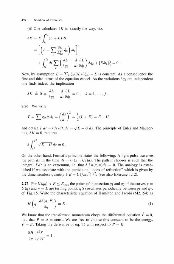
494 Solution of Exercises
(ii) One calculates δK in exactly the way, viz.
δK = K∫ t2
t1
(L+ E) dt
=[(L−
∑k
∂L
∂qkqk
)δti
]t2t1
+∫ t2
t1
dt∑k
(∂L
∂qk− d
dt
∂L
∂qk
)δqk + [Eδti]t2t1 = 0 .
Now, by assumption E =∑k qk(∂L/∂qk)−L is constant. As a consequence the
first and third terms of the equation cancel. As the variations δqk are independentone finds indeed the implication
δK!= 0 ⇔ ∂L
∂qk− d
dt
∂L
∂qk= 0 , k = 1, . . . , f .
2.26 We write
T =∑gikqi qk =
(ds
dt
)2
= 1
2(L+ E) = E − U
and obtain T dt = (ds/dt)ds = √E − U ds. The principle of Euler and Mauper-tuis, δK = 0, requires
δ
∫ q2
q1
√E − U ds = 0 .
On the other hand, Fermat’s principle states the following: A light pulse traversesthe path ds in the time dt = (n(x, ν)/c)ds. The path it chooses is such that theintegral
∫dt is an extremum, i.e. that δ
∫n(x, ν)ds = 0. The analogy is estab-
lished if we associate with the particle an “index of refraction” which is given bythe dimensionless quantity ((E − U)/mc2)1/2; (see also Exercise 1.12).
2.27 For U(q0) < E ≤ Emax the points of intersection q1 and q2 of the curves y =U(q) and y = E are turning points, q(t) oscillates periodically between q1 and q2,cf. Fig. 15. Write the characteristic equation of Hamilton and Jacobi (M2.154) as
H
(q,∂S(q, P )
∂q
)= E . (1)
We know that the transformed momentum obeys the differential equation P = 0,i.e., that P = α = const. We are free to choose this constant to be the energy,P = E. Taking the derivative of eq. (1) with respect to P = E,
∂H
∂p
∂2S
∂q ∂P= 1 .
Chapter 2: The Principles of Canonical Mechanics 495
Fig. 15.
If ∂H/∂p = 0 (this holds locally if E is larger than U(q0)), then (∂2S)/(∂q∂P ) =0. Thus, the equation Q = ∂S(q, P )/∂P can be solved locally for q = q(Q,P ).This yields
H
(q(Q,P ),
∂S
∂q(q(Q, P ), P )
)≡ H (Q, P ) = E ≡ P .
From this we conclude
Q = ∂H∂P
= 1 , P = −∂H∂Q
= 0 ⇒ Q = t − t0 = ∂S
∂E.
The integral I (E) becomes
I (E) = 1
2π
∮ΓE
p dq = 1
2π
∫ t0+T (E)
t0
p · q dt
so that dI (E)/dE = T (E)/(2π) ≡ ω(E), in agreement with Exercise 2.1.
2.28 The function S(q, I ), with I as in Exercise 2.27, generates the transforma-tion from (q, p) to the action and angle variables (θ, I ),
p = ∂S(q, I )∂q
, θ = ∂S(q, I )∂I
, with H = E(I) .
We then have θ = ∂E/∂I = const., I = 0, which are integrated to θ(t) =(∂E/∂I)t + θ0, I = const. Call the circular frequency ω(E) := ∂E/∂I so thatθ(t) = ωt + θ0, I = const.
2.29 We calculate the integral I (E) of Exercise 2.27 for the case H = p2/2 +q2/2: With p = √
2E − q2
496 Solution of Exercises
I (E) = 1
2π
∮ΓE
p dq = 1
2π
∮ΓE
√2E − q2 dq
= 1
π
∫ +A
−A
√A2 − q2 dq ,
(A = √2E
).
Using∫ A
−A
√A2 − x2 dx = πA
2
2
one finds I (E) = A2/2 = E, i.e., H = I . The characteristic equation (M2.154)reads in the present example
1
2
(∂S
∂q
)2
+ 1
2q2 = E .
Its solution can be written as an indefinite integral S = ∫ √2E − q ′2 dq ′, or
S(q, I ) = ∫ √2I − q ′2 dq ′. The angle variable follows from this
θ = ∂S∂I=
∫1√
2I − q ′2 dq′ = arcsin
q√2I,
giving q = √2I sin θ . In a similar fashion one calculates
p = ∂S∂q=
√2I − q2 = √2I cos θ .
These are identical with the formulas that follow from the canonical transformationΦ(q,Q) = (q2/2) cotQ, cf. eq. (M2.95).
2.30 Following Exercise 2.17 we take the time variable t to be a generalizedcoordinate t = qf+1 and introduce in its place a new variable τ such that
L
(q, t,
dq
dτ,dt
dτ
):= L
(q,
1
(dt/dτ)
dq
dτ
)dt
dτ.
By assumption f = 1, i.e., q1 = q and q2 ≡ qf+1 = t . The action integral (theprincipal function) with the boundary conditions modified accordingly, reads
I s0 =∫ τ ′2
τ ′1dτ L(φ1(s, τ ), φf+1(s, τ ), φ
′1(s, τ ), φ
′f+1(s, τ )) ,
the prime denoting the derivative with respect to τ . We now take the derivative ofI s0 with respect to s, at s = 0,
d
dsI s0
∣∣∣∣s=0
=∫ τ2
τ1
dτ
×∂L
∂φ1
dφ1
ds+ ∂L
∂φ′1
dφ′1ds
+ ∂L
∂φf+1
dφf+1
ds+ ∂L
∂φ′f+1
dφ′f+1
ds
. (1)
Chapter 3: The Mechanics of Rigid Bodies 497
Replacing ∂L/∂φ1 in the first term by (d/dτ)(∂L/∂φ′1), through the equations ofmotion, the first two terms of the curly brackets in eq. (1) can be combined to atotal derivative with respect to τ . The integral over τ can be rewritten as an integralover t , so that the first two terms give the contribution∫ t2
t1
dtd
dt
(∂L
∂φ1
dφ1
ds
)= pb dq
b
ds− pa dq
a
ds.
(Note that here the dot means the derivative with respect to t , as before.) In thethird term we replace ∂L/∂φf+1 by (d/dτ)(∂L/∂φ′f+1), (again by virtue of theequation of motion). In this term and in the last term of the curly brackets in eq. (1)we make use of the solution to Exercise 2.17, viz.
∂L
∂(∂φf+1/∂τ)= ∂L
∂(∂t/∂τ)= L− ∂L
∂φ1
dφ1
dt
so that these terms can also be combined to a total derivative
d
dτ
((L− ∂L
∂φ1
dφ1
dt
)dφf+1
ds
). (2)
As above, in doing the integral one replaces τ by the variable t . The inner bracketin eq. (2) is the energy (to within the sign) so that we obtain the difference of theterm −E(dφf+1/ds) at the two boundary points, that is, (−E) times the deriva-tive of the time t = t2− t1 by s. Summing up one indeed obtains the result of theassertion. Finally, the generalization to f > 1 is obvious.
Chapter 3: The Mechanics of Rigid Bodies
3.1 (i) As K and K differ by a time-dependent rotation, J is related to J byJ = R(t)JR−1(t), with R(t) the rotation matrix that describes the relative rotationof the two coordinate systems. The characteristic polynomial of J is invariant undersimilarity transformations. Indeed, by the multiplication law for determinants,
det |J− λ1l| = det∣∣∣R(t)JR−1(t)− λ1l
∣∣∣= det
∣∣∣R(t)(J− λ1l)R−1(t)
∣∣∣= det
∣∣∣J− λ1l∣∣∣ .
The characteristic polynomials of J and J are the same. Hence, their eigenvaluesare pairwise equal.
(ii) If K is a principal-axes system, J has the form
J =⎧⎪⎪⎪⎪⎪⎪⎩I1 0 0
0 I2 00 0 I3
⎫⎪⎪⎪⎪⎪⎪⎭ .
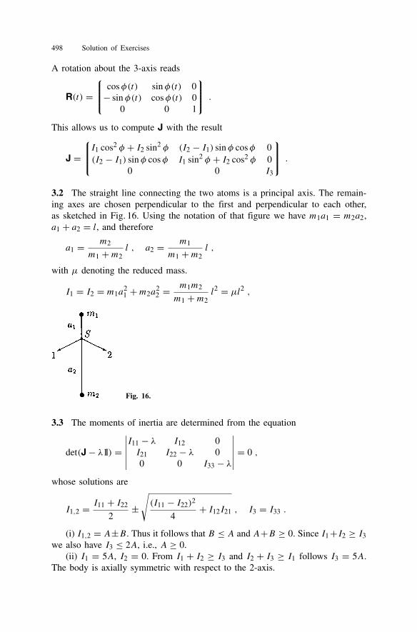
498 Solution of Exercises
A rotation about the 3-axis reads
R(t) =⎧⎪⎪⎪⎪⎪⎪⎩ cosφ(t) sin φ(t) 0− sin φ(t) cosφ(t) 0
0 0 1
⎫⎪⎪⎪⎪⎪⎪⎭ .
This allows us to compute J with the result
J =⎧⎪⎪⎪⎪⎪⎪⎩I1 cos2 φ + I2 sin2 φ (I2 − I1) sin φ cosφ 0(I2 − I1) sin φ cosφ I1 sin2 φ + I2 cos2 φ 0
0 0 I3
⎫⎪⎪⎪⎪⎪⎪⎭ .
3.2 The straight line connecting the two atoms is a principal axis. The remain-ing axes are chosen perpendicular to the first and perpendicular to each other,as sketched in Fig. 16. Using the notation of that figure we have m1a1 = m2a2,a1 + a2 = l, and therefore
a1 = m2
m1 +m2l , a2 = m1
m1 +m2l ,
with µ denoting the reduced mass.
I1 = I2 = m1a21 +m2a
22 =
m1m2
m1 +m2l2 = µl2 ,
Fig. 16.
3.3 The moments of inertia are determined from the equation
det(J− λ1l) =∣∣∣∣∣∣I11 − λ I12 0I21 I22 − λ 00 0 I33 − λ
∣∣∣∣∣∣ = 0 ,
whose solutions are
I1,2 = I11 + I22
2±√(I11 − I22)2
4+ I12I21 , I3 = I33 .
(i) I1,2 = A±B. Thus it follows that B ≤ A and A+B ≥ 0. Since I1+I2 ≥ I3we also have I3 ≤ 2A, i.e., A ≥ 0.
(ii) I1 = 5A, I2 = 0. From I1 + I2 ≥ I3 and I2 + I3 ≥ I1 follows I3 = 5A.The body is axially symmetric with respect to the 2-axis.
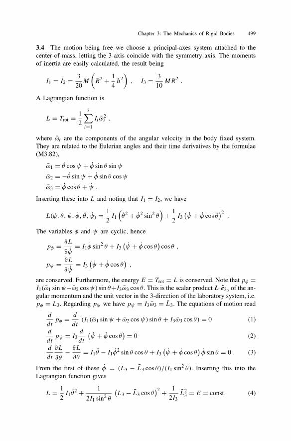
Chapter 3: The Mechanics of Rigid Bodies 499
3.4 The motion being free we choose a principal-axes system attached to thecenter-of-mass, letting the 3-axis coincide with the symmetry axis. The momentsof inertia are easily calculated, the result being
I1 = I2 = 3
20M
(R2 + 1
4h2), I3 = 3
10MR2 .
A Lagrangian function is
L = Trot = 1
2
3∑i=1
Iiω2i ,
where ωi are the components of the angular velocity in the body fixed system.They are related to the Eulerian angles and their time derivatives by the formulae(M3.82),
ω1 = θ cosψ + φ sin θ sinψ
ω2 = −θ sinψ + φ sin θ cosψ
ω3 = φ cos θ + ψ .Inserting these into L and noting that I1 = I2, we have
L(φ, θ, ψ, φ, θ , ψ) = 1
2I1
(θ2 + φ2 sin2 θ
)+ 1
2I3(ψ + φ cos θ
)2.
The variables φ and ψ are cyclic, hence
pφ = ∂L∂φ
= I1φ sin2 θ + I3(ψ + φ cos θ
)cos θ ,
pψ = ∂L
∂ψ= I3
(ψ + φ cos θ
),
are conserved. Furthermore, the energy E = Trot = L is conserved. Note that pφ =I1(ω1 sinψ+ω2 cosψ) sin θ+I3ω3 cos θ . This is the scalar product L·e30 of the an-gular momentum and the unit vector in the 3-direction of the laboratory system, i.e.pφ = L3. Regarding pψ we have pψ = I3ω3 = L3. The equations of motion read
d
dtpφ = d
dt(I1(ω1 sinψ + ω2 cosψ) sin θ + I3ω3 cos θ) = 0 (1)
d
dtpψ = I3 d
dt
(ψ + φ cos θ
) = 0 (2)
d
dt
∂L
∂θ− ∂L∂θ= I1θ − I1φ2 sin θ cos θ + I3
(ψ + φ cos θ
)φ sin θ = 0 . (3)
From the first of these φ = (L3 − L3 cos θ)/(I1 sin2 θ). Inserting this into theLagrangian function gives
L = 1
2I1θ
2 + 1
2I1 sin2 θ
(L3 − L3 cos θ
)2 + 1
2I3L2
3 = E = const. (4)
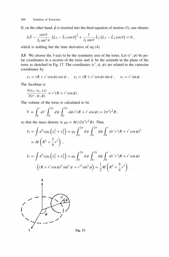
500 Solution of Exercises
If, on the other hand, φ is inserted into the third equation of motion (3), one obtains
I1θ − cos θ
I1 sin3 θ
(L3 − L3 cos θ
)2 + 1
I1 sin θL3
(L3 − L3 cos θ
) = 0 ,
which is nothing but the time derivative of eq. (4).
3.5 We choose the 3-axis to be the symmetry axis of the torus. Let (r ′, φ) be po-lar coordinates in a section of the torus and ψ be the azimuth in the plane of thetorus as sketched in Fig. 17. The coordinates (r ′, ψ, φ) are related to the cartesiancoordinates by
x1 = (R + r ′ cosφ) cosψ , x2 = (R + r ′ cosφ) sinψ , x3 = r ′ sin φ .
The Jacobian is
∂(x1, x2, x3)
∂(r ′, ψ, φ)= r ′(R + r ′ cosφ) .
The volume of the torus is calculated to be
V =∫ r
0dr ′
∫ 2π
0dψ
∫ 2π
0dφ r ′(R + r ′ cosφ) = 2π2r2R ,
so that the mass density is 0 = M/(2π2r2R). Thus
I3 =∫d3x0
(x2
1 + x22
)= 0
∫ 2π
0dψ
∫ 2π
0dφ
∫ r
0dr ′ r ′(R + r ′ cosφ)3
= M(R2 + 3
4r2),
I1 =∫d3x0
(x2
2 + x23
)= 0
∫ 2π
0dψ
∫ 2π
0dφ
∫ r
0dr ′ r ′(R + r ′ cosφ)
·((R + r ′ cosφ)2 sin2 ψ + r ′2 sin2 φ
)= 1
2M
(R2 + 5
4r2).
Fig. 17.
Chapter 3: The Mechanics of Rigid Bodies 501
Fig. 18.
3.6 In the first position we have I (a)3 = 2(2/5)(MR2+mr2) and ω(a)3 = L3/I(a)3 .
In the second position the contribution of the two smaller balls is calculated bymeans of Steiner’s theorem, I ′i = Ii + m(a2 − a2
i ), now with I3 = 2mr2/5,a = ±(b/2)e1:
I(b)3 = 2
((2/5)(MR2 +mr2)+mb2/4
).
It follows that ω(b)3 = L3/I(b)3 , and ω(a)3 /ω
(b)3 = 1 + mb2/(2I (a)3 ). One rotates
faster if the arms are close to one’s body than if they are stretched out. Makinguse of Steiner’s theorem once more we finally calculate I1 = I2. For the two ar-rangements one obtains the result
I(a)1 = I (a)3 + 1
2a2
(M + 1
9m
), I
(b)1 = 4
5
(MR2 +mr2
)+ 5
9Ma2 .
3.7 The relation between density and mass reads
M =∫(r) d3r =
∫ 2π
0dφ
∫ π
0sin θ dθ
∫ ∞
0r2 dr (r, θ, φ) .
In our case, where depends on θ only, this means
M =∫ 2π
0dφ
∫ π
0sin θ dθ
∫ R(θ)
0r2 dr 0 = 2π
30
∫ π
0sin θ dθ R(θ)3 .
The moments of inertia I3, I1 = I2 are calculated from the formulas
I3 =∫
d3x r2(1− cos2 θ) , I1 + I2 + I3 = 2∫
d3x r2 ,
(i) Integration gives the results
M = 4π
30R
30(1+ α)2 , i.e., 0 = 3
4π
M
R30(1+ α2)
.
I1 = I2 = 2MR20
5(1+ α2)
1+ 4α2 + 9
7α4, I3 = 2MR2
0
5(1+ α2)
1+ 2α2 + 3
7α4.
(ii) Substituting z = cos θ the integrals are easily evaluated. With the abbrevi-ation γ := √5/16π β we obtain
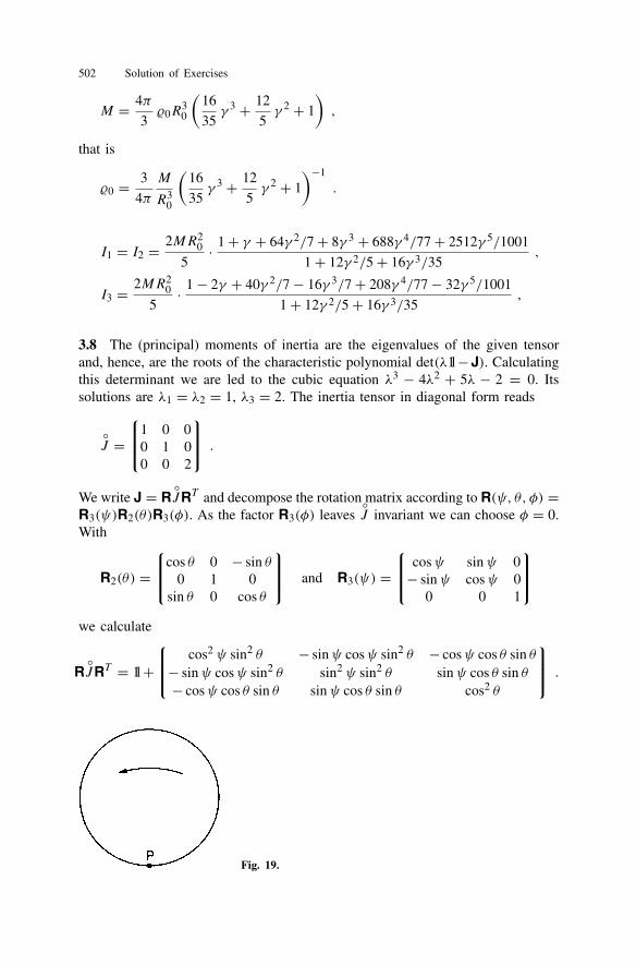
502 Solution of Exercises
M = 4π
30R
30
(16
35γ 3 + 12
5γ 2 + 1
),
that is
0 = 3
4π
M
R30
(16
35γ 3 + 12
5γ 2 + 1
)−1
.
I1 = I2 = 2MR20
5· 1+ γ + 64γ 2/7+ 8γ 3 + 688γ 4/77+ 2512γ 5/1001
1+ 12γ 2/5+ 16γ 3/35,
I3 = 2MR20
5· 1− 2γ + 40γ 2/7− 16γ 3/7+ 208γ 4/77− 32γ 5/1001
1+ 12γ 2/5+ 16γ 3/35,
3.8 The (principal) moments of inertia are the eigenvalues of the given tensorand, hence, are the roots of the characteristic polynomial det(λ1l−J). Calculatingthis determinant we are led to the cubic equation λ3 − 4λ2 + 5λ − 2 = 0. Itssolutions are λ1 = λ2 = 1, λ3 = 2. The inertia tensor in diagonal form reads
J =
⎧⎪⎪⎪⎪⎪⎪⎩1 0 00 1 00 0 2
⎫⎪⎪⎪⎪⎪⎪⎭ .
We write J = RJRT and decompose the rotation matrix according to R(ψ, θ, φ) =
R3(ψ)R2(θ)R3(φ). As the factor R3(φ) leavesJ invariant we can choose φ = 0.
With
R2(θ) =⎧⎪⎪⎪⎪⎪⎪⎩cos θ 0 − sin θ
0 1 0sin θ 0 cos θ
⎫⎪⎪⎪⎪⎪⎪⎭ and R3(ψ) =⎧⎪⎪⎪⎪⎪⎪⎩ cosψ sinψ 0− sinψ cosψ 0
0 0 1
⎫⎪⎪⎪⎪⎪⎪⎭we calculate
RJRT = 1l+
⎧⎪⎪⎪⎪⎪⎪⎩cos2 ψ sin2 θ − sinψ cosψ sin2 θ − cosψ cos θ sin θ
− sinψ cosψ sin2 θ sin2 ψ sin2 θ sinψ cos θ sin θ− cosψ cos θ sin θ sinψ cos θ sin θ cos2 θ
⎫⎪⎪⎪⎪⎪⎪⎭ .
Fig. 19.
Chapter 3: The Mechanics of Rigid Bodies 503
If this is set equal to J as given, we find cos2 θ = 3/8, and, with the followingchoice of signs for θ : cos θ = √
3/(2√
2) and sin θ = √5/(2
√2), the result
cosψ = 1/√
5, sinψ = −√4/5.
3.9 (i) (r) = 0θ(a − |r|). The total mass is equal to the volume integral of(r), viz.
M = 4π
3a30 ⇒ 0 = 3M
4πa3.
(ii) We choose the 3-axis to be the axis of rotation. Let the coordinate in thebody fixed system be (x, y, z), the coordinates in the space fixed system are
x′ = x cosωt − (y + a) sinωt , y′ = x sinωt + (y + a) cosωt , z′ = z .Inverting these equations we have
x = +x′ cosωt + y′ sinωt , y = −x′ sinωt + y′ cosωt − a ,whence
x2 + y2 = x′2 + y′2 + a2 + 2a(x′ sinωt − y′ cosωt) .
From this we get
(r ′, t) = 0θ(a −
√r ′2 + a2 + 2a(x′ sinωt − y′ cosωt)
).
(iii) In the case of a homogeneous sphere the inertia tensor is diagonal, allthree moments of inerta are equal, I1 = I2 = I3 ≡ I . Hence,
3I = I1 + I2 + I3 = 2∫d3r(r)r2 = 6Ma2
5.
Making use of Steiner’s theorem (M3.23) we find
I ′3 = I3 +M(a2δ33 − a2
3
)= 7Ma2
5.
3.10 (i) The volume of the cylinder is V = πr2h, hence the mass density is0 = m/(πr2h). The moment of inertia relevant for rotations about the symmetryaxis is best calculated using cylindrical coordinates,
I3 = 0
∫ 2π
0dφ
∫ h
0dz
∫ r
03 d = 1
2mr2 .
Call q(t) the projection of the center-of-mass’ orbit onto the inclined plane. Whenthe center-of-mass moves by an amount dq, the cylinder rotates by an angledφ = dq/r . Therefore, the total kinetic energy is
T = 1
2mq2 + 1
2I3q2
r2= 3
4mq2 .
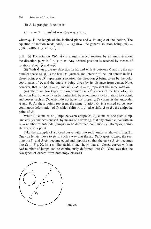
504 Solution of Exercises
(ii) A Lagrangian function is
L = T − U = 3mq2/4−mg(q0 − q) sin α ,
where q0 is the length of the inclined plane and α its angle of inclination. Theequation of motion reads 3mq/2 = mg sin α, the general solution being q(t) =q(0)+ v(0)t + (g sin α)t2/3.
3.11 (i) The rotation R(φ · φ) is a right-handed rotation by an angle φ aboutthe direction φ, with 0 ≤ φ ≤ π . Any desired position is reached by means ofrotations about φ and −φ.
(ii) With φ an arbitrary direction in R, and with φ between 0 and π , the pa-rameter space (φ, φ) is the ball D3 (surface and interior of the unit sphere in R3).Every point p ∈ D3 represents a rotation, the direction φ being given by the polarcoordinates of p, and the angle φ being given by its distance from center. Note,however, that A : (φ, φ = π) and B : (−φ, φ = π) represent the same rotation.
(iii) There are two types of closed curves in D3: curves of the type of C1 asshown in Fig. 20, which can be contracted, by a continuous deformation, to a point,and curves such as C2, which do not have this property. C2 connects the antipodesA and B. As these points represent the same rotation, C2 is a closed curve. Anycontinuous deformation of C2 which shifts A to A′ also shifts B to B ′, the antipodalpoint of A′.
While C1 contains no jumps between antipodes, C2 contains one such jump.One easily convinces oneself, by means of a drawing, that any closed curve with aneven number of antipodal jumps can be deformed continuously into C1 or, equiv-alently, into a point.
Take the example of a closed curve with two such jumps as shown in Fig. 21.One can let A1 move to B2 in such a way that the arc B1A2 goes to zero, the sec-tions A1B1 and A2B2 become equal and opposite so that the curve A1B2 becomeslike C1 in Fig. 20. In a similar fashion one shows that all closed curves with anodd number of jumps can be continuously deformed into C2. (One says that thetwo types of curves form homotopy classes.)
Fig. 20.
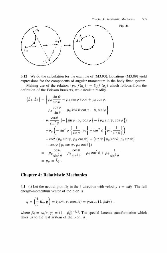
Chapter 4: Relativistic Mechanics 505
Fig. 21.
3.12 We do the calculation for the example of (M3.93). Equations (M3.89) yieldexpressions for the components of angular momentum in the body fixed system.
Making use of the relation pi, f (qj ) = δij f ′(qj ) which follows from thedefinition of the Poisson brackets, we calculate readily
L1, L2 =
pφsinψ
sin θ− pψ sinψ cot θ + pθ cosψ,
pφcosψ
sin θ− pψ cosψ cot θ − pθ sinψ
= pθ cos θ
sin2 θ
(− sinψ,pψ cosψ
− pψ sinψ, cosψ
)+pφ
(− sin2 ψ
1
sin θ, pθ
+ cos2 ψ
pθ ,
1
sin θ
)+ cot2 (pψ sinψ,pψ cosψ
+ (sinψ
pψ cot θ, pθ sinψ
− cosψ
pθ cosψ,pψ cot θ
)= +pφ cos θ
sin2 θ− pφ cos θ
sin2 θ− pψ cot2 θ + pψ 1
sin2 θ
= pψ = L3 .
Chapter 4: Relativistic Mechanics
4.1 (i) Let the neutral pion fly in the 3-direction with velocity v = v0e3. The fullenergy–momentum vector of the pion is
q =(
1
cEq, q
)= (γ0mπc, γ0mπv) = γ0mπc
(1, β0e3
),
where β0 = v0/c, γ0 = (1 − β20 )−1/2. The special Lorentz transformation which
takes us to the rest system of the pion, is
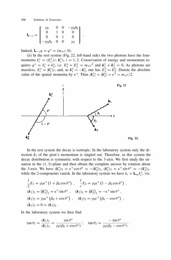
506 Solution of Exercises
L−v =
⎧⎪⎪⎪⎪⎪⎪⎪⎪⎪⎩γ0 0 0 −γ0β00 1 0 00 0 1 0
−γ0β0 0 0 γ0
⎫⎪⎪⎪⎪⎪⎪⎪⎪⎪⎭ .
Indeed, L−vq = q∗ = (mπc, 0).(ii) In the rest system (Fig. 22, left-hand side) the two photons have the four-
momenta k∗i = (E∗i /c, k∗i ), i = 1, 2. Conservation of energy and momentum re-quires q∗ = k∗1 + k∗2 , i.e. E∗1 + E∗2 = mπc2 and k∗1 + k∗2 = 0. As photons aremassless, E∗i = |k∗i |c, and, as k∗1 = −k∗2, one has E∗1 = E∗2 . Denote the absolutevalue of the spatial momenta by κ∗. Then |k∗1| = |k∗2| = κ∗ = mπc/2.
Fig. 22.
In the rest system the decay is isotropic. In the laboratory system only the di-rection e3 of the pion’s momentum is singled out. Therefore, in this system thedecay distribution is symmetric with respect to the 3-axis. We first study the sit-uation in the (1, 3)-plane and then obtain the complete answer by rotation aboutthe 3-axis. We have (k∗1)3 = κ∗ cos θ∗ = −(k∗2)3, (k∗1)1 = κ∗ sin θ∗ = −(k∗2)1,while the 2-components vanish. In the laboratory system we have ki = Lv0k
∗i , viz.
1
2E1 = γ0κ
∗ (1+ β0 cos θ∗),
1
cE2 = γ0κ
∗ (1− β0 cos θ∗),
(k1)1 =(k∗1)
1 = κ∗ sin θ∗ , (k2)1 =(k∗2)
1 = −κ∗ sin θ∗ ,
(k1)3 = γ0κ∗ (β0 + cos θ∗
), (k2)3 = γ0κ
∗ (β0 − cos θ∗),
(k1)2 = 0 = (k2)2 .
In the laboratory system we then find
tan θ1 = (k1)1
(k1)3= sin θ∗
γ0(β0 + cos θ∗); tan θ2 = − sin θ∗
γ0(β0 − cos θ∗).
Chapter 4: Relativistic Mechanics 507
Examples:
a) θ∗ = 0 (forward emission of one photon, backward emission of the other): Fromthe formulas above one finds E1 = mπc2γ0(1+ β0)/2, E2 = mπc2γ0(1− β0)/2,k1 = mπcγ0(β0 + 1)e3/2, k2 = mπcγ0(β0 − 1)e3/2, and, as β0 ≤ 1, θ1 = 0,θ2 = π .
b) θ∗ = π/2 (transverse emission): In this case E1 = E2 = mπc2γ0/2, k1 =mπc(e1 + γ0β0e3)/2, k2 = mπc(−e1 + γ0β0ee)/2, tan θ1 = tan θ2 = 1/(γ0β0).
c) θ∗ = π/4 and β0 = 1/√
2, i.e, γ0 =√
2: In this case one finds E1 =3mπc2γ0/4, E2 = mπc
2γ0/4, k1 = mπc(e1 − 2√
2e3)/(2√
2), k2 =−mπce1/(2
√2), θ1 = arctan(1/(2
√2)) ≈ 0.108π , θ2 = π/2.
In the rest system the decay distribution is isotropic, which means that thedifferential probability dΓ for k∗1 to lie in the interval dΩ∗ = sin θ∗ dθ∗ dφ∗ isindependent of θ∗ and of φ∗. (To see this enclose the decaying pion by a unitsphere. If one considers a large number of decays then photon 1 will hit everysurface element dΩ∗ on that sphere with equal probability.) Thus,
dΓ = Γ0 dΩ∗ with Γ0 = const.
In the laboratory system the analogous distribution is no longer isotropic. It is dis-torted in the direction of flight but is still axially symmetric about that axis. Wehave
1
Γ0dΓ =
∣∣∣∣dΩ∗dΩ
∣∣∣∣ dΩ wheredΩ∗
dΩ= sin θ∗
sin θ
dθ∗
dθ.
The factor sin θ∗/ sin θ is calculated from the above formula for tan θ1, viz.
sin θ = tan θ√1+ tan2 θ
= sin θ∗
γ0(β0 + cos θ∗),
and the derivative dθ/dθ∗ is obtained from θ = arctan(sin θ∗/γ0(β0+ cos θ∗)) bymaking use of the relation γ 2
0 β20 = γ 2
0 − 1. One finds
dΩ∗
dΩ= γ 2
0
(1+ β0 cos θ∗
)2.
The cosine of θ∗ is expressed in terms of the corresponding laboratory angle bythe formula
cos θ∗ = cos θ − β0
1− β0 cos θ.
The shift of the angular distribution is well illustrated by the graph of the function
F(θ) := dΩ∗
dΩ= γ 2
0
(1+ β0
cos θ − β0
1− β0 cos θ
)2
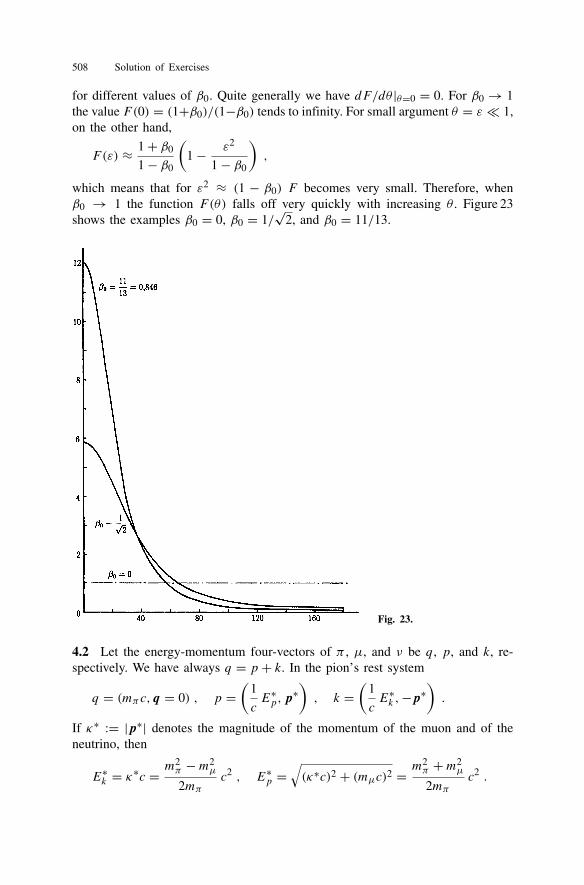
508 Solution of Exercises
for different values of β0. Quite generally we have dF/dθ |θ=0 = 0. For β0 → 1the value F(0) = (1+β0)/(1−β0) tends to infinity. For small argument θ = ε 1,on the other hand,
F(ε) ≈ 1+ β0
1− β0
(1− ε2
1− β0
),
which means that for ε2 ≈ (1 − β0) F becomes very small. Therefore, whenβ0 → 1 the function F(θ) falls off very quickly with increasing θ . Figure 23shows the examples β0 = 0, β0 = 1/
√2, and β0 = 11/13.
Fig. 23.
4.2 Let the energy-momentum four-vectors of π , µ, and ν be q, p, and k, re-spectively. We have always q = p + k. In the pion’s rest system
q = (mπc, q = 0) , p =(
1
cE∗p,p∗
), k =
(1
cE∗k ,−p∗
).
If κ∗ := |p∗| denotes the magnitude of the momentum of the muon and of theneutrino, then
E∗k = κ∗c =m2π −m2
µ
2mπc2 , E∗p =
√(κ∗c)2 + (mµc)2 =
m2π +m2
µ
2mπc2 .
Chapter 4: Relativistic Mechanics 509
In the laboratory system the situation is as follows: The pion has velocity v0 = v0e3and, therefore,
q = (Eq/c, q) = (γ0mπc, γ0mπv0) = γ0mπc(1, β0e3)
with β0 = v0/c, γ0 = 1/√
1− β20 . It is sufficient to study the kinematics in the
(1, 3)-plane. The transformation from the pion’s rest system to the laboratory sys-tem yields
1
cEp = γ0
(1
cE∗p + β0p
∗3)= γ0
(1
cE∗p + β0κ
∗ cos θ∗),
p1 = p∗1 ,
p2 = p∗2 = 0 ,
p3 = γ0
(1
cβ0E
∗0 + p∗3
)= γ0
(1
cβ0E
∗p + κ∗ cos θ∗
)and, therefore, the relation between the angles of emission θ∗ and θ is (cf. Fig. 24)
tan θ = p1
p3= κ∗ sin θ∗
γ0(β0E∗p/c + κ∗ cos θ∗), (1)
or
tan θ =(m2π −m2
µ
)sin θ∗
γ0(β0
(m2π +m2
µ
)+ (m2π −m2
µ
)cos θ∗
) . (2)
Fig. 24.
Making use of β∗ := cκ∗/E∗p = (m2π − m2
µ)/(m2π + m2
µ) (this is the beta factorof the muon in the rest system of the pion), eq. (1) is rewritten
tan θ = β∗ sin θ∗
γ0(β0 + β∗ cos θ∗). (3)
There exists a maximal angle θ if the muons which are emitted backwards in thepion’s rest system (θ∗ = π), have momenta
p3 = γ0E∗p/c
(β0 + β∗ cos θ∗
) = γ0E∗p/c
(β0 − β∗
)> 0 ,
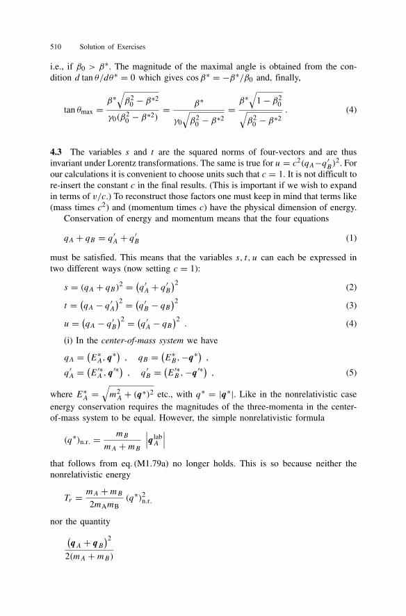
510 Solution of Exercises
i.e., if β0 > β∗. The magnitude of the maximal angle is obtained from the con-
dition d tan θ/dθ∗ = 0 which gives cosβ∗ = −β∗/β0 and, finally,
tan θmax =β∗
√β2
0 − β∗2
γ0(β20 − β∗2)
= β∗
γ0
√β2
0 − β∗2=β∗
√1− β2
0√β2
0 − β∗2. (4)
4.3 The variables s and t are the squared norms of four-vectors and are thusinvariant under Lorentz transformations. The same is true for u = c2(qA−q ′B)2. Forour calculations it is convenient to choose units such that c = 1. It is not difficult tore-insert the constant c in the final results. (This is important if we wish to expandin terms of v/c.) To reconstruct those factors one must keep in mind that terms like(mass times c2) and (momentum times c) have the physical dimension of energy.
Conservation of energy and momentum means that the four equations
qA + qB = q ′A + q ′B (1)
must be satisfied. This means that the variables s, t, u can each be expressed intwo different ways (now setting c = 1):
s = (qA + qB)2 =(q ′A + q ′B
)2 (2)
t = (qA − q ′A
)2 = (q ′B − qB
)2 (3)
u = (qA − q ′B
)2 = (q ′A − qB
)2. (4)
(i) In the center-of-mass system we have
qA =(E∗A, q∗
), qB =
(E∗B,−q∗
),
q ′A =(E′∗A , q ′∗
), q ′B =
(E′∗B ,−q ′∗
), (5)
where E∗A =√m2A + (q∗)2 etc., with q∗ = |q∗|. Like in the nonrelativistic case
energy conservation requires the magnitudes of the three-momenta in the center-of-mass system to be equal. However, the simple nonrelativistic formula
(q∗)n.r. = mB
mA +mB∣∣∣q labA
∣∣∣that follows from eq. (M1.79a) no longer holds. This is so because neither thenonrelativistic energy
Tr = mA +mB2mAmB
(q∗)2n.r.
nor the quantity(qA + qB
)2
2(mA +mB)
Chapter 4: Relativistic Mechanics 511
are conserved. We have
s = (E∗A + E∗B
)2 = m2A +m2
B + 2(q∗)2
+2√((q∗)2 +m2
A
) ((q∗)2 +m2
B
). (6)
Thus, s is the square of the total energy in the center-of-mass system. Reintroduc-ing the velocity of light,
s = m2Ac
4 +m2Bc
4 + 2(q∗)2c2 + 2√((q∗)2c2 +m2
Ac4) ((q∗)2c2 +m2
Bc4).
In a first step we check that s, when expanded in terms of 1/c, gives the correctnonrelativistic kinetic energy Tr of relative motion (except for the rest masses, ofcourse)
s ≈(mAc
2 +mBc2)2
(1+ 1
mAmB(q∗)2/c2 +O
((q∗)4
m4c4
)),
and, thus,
√s ≈ mAc2 +mBc2 + mA +mB
2mAmB(q∗)2 +O
((q∗c)4
(mc2)4
).
The magnitude of the center-of-mass momentum is obtained from (6)
q∗(s) = 1
2√s
√(s − (mA +mB)2
) (s − (mA −mB)2
). (7)
Clearly, the reaction can take place only if s is at least equal to the square of thesum of the rest energies,
s ≥ s0 := (mA +mB)2 =(mAc
2 +mBc2)2.
s0 is called the threshold of the reaction. For s = s0 the momentum vanishes,which means that at threshold the kinetic energy of relative motion vanishes.
The variable t is expressed in terms of q∗ and the scattering angle θ∗ as follows:
t = (qA − q ′A
)2 = q2A + q ′2A − 2qA · q ′A = 2m2
A − 2E∗AE′∗A + 2q∗ · q ′∗ .As the magnitudes of q∗ and of q ′∗ are equal, E∗A = E∗B . Therefore,
t = −2(q∗)2(1− cos θ∗) . (8)
Except for the sign, t is the square of the momentum transfer (q∗ − q ′∗) in thecenter-of-mass system. For fixed s ≥ s0, t varies as follows
−4(q∗)2 ≤ t ≤ 0 .
512 Solution of Exercises
Examples:
a) e− + e− → e− + e−
s ≥ s0 = 4(mec
2)2, −(s − s0) ≤ t ≤ 0 .
b) ν + e− → e− + νs ≥ s0 =
(mec
2)2, −1
s(s − s0)2 ≤ t ≤ 0 .
(ii) Calculating s+ t +u from the formulas (2)–(4) and making use of (1), wefind s+ t+u = 2(m2
A+m2B)c
4. More generally, for the reaction A+B → C+D,one finds
s + t + u =(m2A +m2
B +m2C +m2
D
)c4 .
4.4 In the laboratory system
qA =(EA, qA
), qB =
(mBc
2, 0),
q ′A =(E′A, q ′A
), q ′B =
(E′B, q ′B
), (1)
The scattering angle θ is the angle between the three-vectors qA and q ′A. Fromeq. (3) of the solution to Exercise 4.3 above (using c = 1),
t = q2A + q ′2A − 2qAq
′A = 2m2
A − 2EAE′A + 2
∣∣qA∣∣ ∣∣q ′A∣∣ cos θ . (2)
Equation (8) of Exercise 4.3 above gives an alternative expression for t . Theaim is now to express the laboratory quantities EA, E′A,
∣∣qA∣∣, ∣∣q ′A∣∣ in termsof the invariants s and t . Using (1) s is found to be, in the laboratory system,s = m2
A +m2B + 2EAmB , that is,
EA = 1
2mB
(s −m2
A −m2B
). (3)
From this, using q2A = E2
A −m2A,∣∣qA∣∣ = 1
2mB
√(s − (mA +mB)2
) (s − (mA −mB)2
) = 1
mBq∗√s (4)
with q∗ as given by eq. (7) of Exercise 4.3 above. We now calculate t = (qB−q ′B)2in the laboratory system and find E′B = (2m2
B − t)/(2mB) and from this E′A =EA +mB − E′B to be equal to
E′A =1
2mB
(s + t −m2
A −m2B
)= EA + t
2mB, (5)
and, eventually, from q ′2A = E′2A −m2A∣∣q ′A∣∣ = 1
2mB
√(s + t − (mA +mB)2
) (s + t − (mA −mB)2
). (6)
Chapter 4: Relativistic Mechanics 513
From (2)
cos θ =(EAE
′A −m2
A +t
2
)1∣∣qA∣∣ ∣∣q ′A∣∣ .
This is used to calculate sin θ and tan θ , replacing all quantities which are not in-variants by the expressions (3)–(6). With the abbreviations Σ := (mA+mB)2 and∆ := (mA −mB)2 we find
tan θ = 2mB√−t (st + (s −Σ)(s −∆))
(s −Σ)(s −∆)+ t (s −m2A +m2
B
) .Finally, cos θ∗ and sin θ∗ can also be expressed in terms of s and t , starting fromeqs. (8) and (7) of Exercise 4.3 above,
cos θ∗ = 2st + (s −Σ) (s −∆)(s −Σ)(s −∆) ,
sin θ∗ = 2√s
√−t (st + (s −Σ)(s −∆))(s −Σ)(s −∆) .
Replace the square root in the numerator of tan θ by sin θ∗ and insert t in thedenominator, as a function of cos θ∗, to obtain the final result
tan θ = 2mB√s
s −m2A +m2
B
sin θ∗
cos θ∗ + s +m2A −m2
B
s −m2A +m2
B
(7)
For s ≈ (mA +mB)2 one recovers the nonrelativistic result (M1.80). The case oftwo equal masses is particularly interesting. With mA = mB ≡ m
tan θ = 2m√s
tanθ∗
2.
As√s ≥ 2m the scattering angle θ is always smaller than in the nonrelativistic
situation.
4.5 If we wish to go from the rest system of a particle to another system whereits four-momentum is p = (E/c,p), we have to apply a special Lorentz transfor-mation L(v) with v related to p by p = mγ v. Solving for v,
v = pc√p2 +m2c2
= pc2
E.
Insertion into eq. (M4.41) and application to the vector (0, s) gives
s = L(v)(0, s) =(γ
cs · v, s + γ 2
c2(1+ γ ) v · sv).
As sαpα is a Lorentz scalar, and hence is independent of the frame of referencethat one uses, this quantity may be evaluated most simply in the rest system. It isfound to vanish there and, hence, in any frame of reference.
514 Solution of Exercises
4.6 In either case the coordinate system can be chosen such that the y- and z-components of the four-vector vanish and the x-component is positive, i.e., z =(z0, z1, 0, 0) with z1 > 0, If z0 is smaller than zero we apply the time reversal oper-ation (M4.30) so that, from here on, we assume z0 > 0, without loss of generality.
(i) A light-like vector has z2 = 0 and, hence, z0 = z1. We apply a boost withparameter λ along the x-direction, cf. (M4.39). In order to obtain the desired formof the four-vector we must have
z0 cosh λ− z0 sinh λ = 1 or z0e−λ = 1 ,
from which follows λ = ln z0.(ii) For a space-like vector z2 = (z0)2− (z1)2 < 0, i.e., 0 < z0 < z1. Applying
a boost with parameter λ it is transformed to(z0 cosh λ− z1 sinh λ, z′ cosh λ− z0 sinh λ, 0, 0
).
For the time component to vanish, one must have tanh λ = z0/z1. Calculatingsinh λ and cosh λ from this yields the assertion z1 = √−z2.
4.7 The commutation relations (M4.59) can be summarized as follows, makinguse of the Levi-Civita symbol:[
Jp,Jq] = εpqrJr ,[
Kp,Kq] = −εpqrJr ,[
Jp,Kq] = εpqrKr .
From this one obtains[Ap,Aq
] = εpqrAr ,[Bp,Bq
] = εpqrBr ,[Ap,Bq
] = 0 .
4.8 The explicit calculation gives
PJiP−1 = Ji , PKjP−1 = −Kj .
This corresponds to the fact that space inversion does not alter the sense of rotationbut reverses the direction of motion.
4.9 The commutators (M4.59) read in this basis[J i , J j
]= iεijkJ k ,[
J i , Kj
]= iεijkKk ,[
Ki, Kj
]= −iεijkJ k .
Chapter 4: Relativistic Mechanics 515
The matrix Ji and Kj being real and skew-symmetric, we have for instance(JT
i
)∗ = − (iJi )∗ = iJi = J i .
4.10 This exercise is a special case of Exercise 4.11. The result is obtained fromthere by taking m2 = 0 = m3.
4.11 Energy conservation implies (again taking c = 1)
M = E1 + E2 + E3 =√m2
1 + f 2 +√m2
2 + x2f 2 +√m2
3 + (1− x)2f 2
= M(xf (x)) .The maximum of f (x) is found from the equation
0!= dfdx= −∂M/∂x
∂M/∂f= −fE1
xE3 − (1− x)E2
E2E3 + x2E1E3 + (1− x)2E1E2,
or xE3 = (1 − x)E2. Squaring this equation gives x2(m23 + (1 − x)2f 2) =
(1− x)2(m22 + x2f 2), and from this the condition
x!= m2
m2 +m3.
Taking into account the condition
E3 = 1− xx
E2 = m3
m2E2 ,
one obtains
M − E1 = m2 +m3
m2E2 .
The square of this yields
M2 − 2ME1 +m21 + f 2 = (m2 +m3)
2
m22
(m2
2 +m2
2
(m2 +m3)2f 2
)and from this
(E1)max = 1
2M
(M2 +m2
1 − (m2 +m3)2).
Examples:
(i) µ→ e+ ν1 + ν2 : m2 = m3 = 0, M = mµ, m1 = me. Thus
(Ee)max = 1
2mµ
(m2µ +m2
e
)c2 .
With mµ/me ≈ 206.8 one finds (Ee)max ≈ 104.4mec2.
516 Solution of Exercises
(ii) n → p + e + ν; M = mn, m1 = me, m2 = mp, m3 = 0. Therefore oneobtains
(Ee)max = 1
2mn
(m2
n +m2e −m2
p
)c2 = 1
2mn
((2mn −∆)∆+m2
e
)c2 ,
where ∆ := mn − mp. Inserting numerical values yields (Ee)max ≈ 2.528mec2.Thus γmax = 2.528 and βmax =
√γ 2
max − 1/γmax = 0.918. The electron is highlyrelativistic at the maximal energy.
4.12 The apparent lifetime τ (v) in the laboratory system is related to the reallifetime τ (0) by τ (v) = γ τ (0). During this time the particle, on average, travels adistance
L = vτ (v) = βγ τ (0)c .Now, the product βγ equals |p|c/(mc2), cf. eq. (M4.83), so that for |p| = xmcthere follows the relation
L = xτ (0)c .For pions, for instance, one has τ (0)π c ≈ 780 cm.
4.13 From the results of the preceding exercise we obtain τ (0)n c ≈ 2.7×1013 cm.For E = 10−2mnc
2 one has x = √γ 2 − 1 = 0.142, while for E = 1014mnc
2 onehas x ≈ 1014.
4.14 Let p1, p2 be the energy–momentum four-vectors of the incoming and out-going electron, respectively, and k that of the photon. Energy and momentum con-servation in the reaction e → e + γ requires p1 = p2 + k. Squaring this relationand making use of
p21 = mec
2 = p22 , k2 = 0 ,
one deduces p2 · k = 0. As k is a light-like four-vector this relation can only holdif p2 is light-like, too, i.e., if p2
2 = 0. This is in contradiction with the outgoingelectron being on its mass shell, p2
2 = m2e . Hence, the reaction cannot take place.
4.15 The first inversion leads from xµ to (R2/x2)xµ, the translation that followsleads to R2(xµ/x2 + cµ), and the second inversion, finally, to
x′µ = R4(xµ + x2cµ
)x4
x2R4(x + x2c
)2= xµ + x2cµ
1+ 2(c · x)+ c2x2.
The inversion J leaves invariant the two halves of the time-like hyperboloidx2 = R2, but interchanges those of the space-like hyperboloid x2 = −R2. Theimage of the light-cone by the inversion is at infinity. The light-cone as a wholestays invariant under the combined transformation J T J .
Chapter 5: Geometric Aspects of Mechanics 517
4.16 As L does not depend on q, the equation of motion for this variable reads
d
dt
∂L
∂ q= m d
dt(ψ q) = 0 . (1)
In turn, L is independent of ψ . The condition for the action integral to be extremalleads to the following equation for ψ ,
∂L
∂ψ= 1
2m
(q2 − c2
0ψ2 − 1
ψ2
)= 0 .
The solutions of this equations are
ψ1 = c0√c2
0 − q2, ψ2 = − c0√
c20 − q2
.
Insertion of ψ1 into the Lagrangian function yields
L(q, ψ = ψ1
) = 1
2m(− 2c0
√c2
0 − q2 + 2c20
)= −mc2
0
√1− q2/c2
0 +mc20 .
This is nothing but eq. (M4.97), with c replaced by c0, to which the constant energymc2
0 is added.If we let c0 go to infinity, ψ1 trends to 1 and the Lagrangian function becomes
Lnr = mq2/2, well-known from nonrelativistic motion. One verifies easily that(1) is the correct equation of motion in either case.
The second solution ψ2 must be excluded. Obviously, the additional term
1
2m(ψ − 1)
(q2 − c2
0ψ − 1
ψ
).
which is added to the Lagrangian function Lnr takes care of the requirement thatthe velocity q should not exceed the value c0.
Chapter 5: Geometric Aspects of Mechanics
5.1 We make use of the decomposition (M5.52) forkω and
lω
kω∧ l
ω∑
i1<···<ikωi1...ik
∑j1<···<jl
ωj1...jl dxi1 ∧ . . . ∧ dxik ∧ dxj1 ∧ . . . ∧ dxjl .
The analogous decomposition oflω∧ k
ω (k and l interchanged) is obtained fromthis by shifting first dxj1 , then dxj2 , and so forth up to dxjl , across the productdxi1 ∧ dxi2 ∧ . . . ∧ dxik from the right to the left. Each one of these operationsgives rise to a factor (−)k , so that one obtains the total factor (−)kl .
518 Solution of Exercises
5.2 We calculate
ds2 (ei , ej ) = 3∑k=1
Ek dxk(ei ) dx
k(ej ) =3∑k=1
Ekaki akj ,
where we have set aki := dxk(ei ). As ds2(ei , ek) = δik , we must have aki =bki /√Ek , where bki is an orthogonal matrix. This matrix must be orthogonal be-
cause the coordinate axes were chosen orthogonal. Therefore dxk(ei ) = δki /√Ek .
5.3 Consider
1ωa =
3∑i=1
ωi(x) dxi ,
2ωa = b1(x) dx
2 ∧ dx3 + cyclic permutations
whose coefficients, ωi(x) and bi(x), are to be determined.a) We calculate
1ωa(ξ) =
∑i
ωi(x) dxi(ξ) =
∑i
ωi(x) dxi
(∑k
ξk ek
)=
∑i
ωi(x)ξi 1√Ei.
Since, on the other hand,
1ωa(ξ) = a · ξ =
∑i
ai(x)ξi
we deduce
ωi(x) = ai(x)√Ei .
b) We calculate
2ωa(ξ , η) = b1(x)(dx
2(ξ) dx3(η)− dx2(η) dx3(ξ))+ cycl. perms.
= b1(x)(ξ2η3 − η2ξ3)/
√E2E3 + cycl. perms. .
Comparing this with the scalar product of a and ξ × η yields
b1(x) =√E2E3 a1(x) (cyclic permutations) .
5.4 Denote by (∇f )i the components of ∇f with respect to the orthogonal basisthat we consider. We then have, according to the solution of Exercise 5.3,
1ω∇f =
∑i
(∇f )i√Ei dx
i .
Chapter 5: Geometric Aspects of Mechanics 519
With ξ = ∑i ξi ei a unit vector, the function
1ω∇f (ξ) = ∑
i (∇f )iξ i is the di-
rectional derivative of f along the direction ξ . This quantity can be calculatedalternatively from the total differential
df =∑i
∂f
∂xidxi
to be
df (ξ) =∑i,k
∂f
∂xiξk dxi (ek) =
∑i
1√Ei
∂f
∂xiξ i .
Comparing the two expressions yields the result
(∇f )i =1√Ei
∂f
∂xi.
5.5 For cartesian coordinates we have E1 = E2 = E3 = 1.For cylindrical coordinates (e, eφ, ez) we have ds2 = d2 + 2dφ2 + dz2,
i.e., E1 = E3 = 1, E2 = 2 and, therefore,
∇f =(∂f
∂,
1
∂f
∂φ,∂f
∂z
).
For spherical coordinates (er , eθ , eφ) we have ds2 = dr2 + r2dθ2 + r sin2 θdφ2,which means that E1 = 1, E2 = r2, E3 = r2 sin2 θ and, hence,
∇f =(∂f
∂r,
1
r
∂f
∂θ,
1
r sin θ
∂f
∂φ
).
5.6 The defining equation (M5.58) can be written alternatively as follows
(∗ω)(eik+1 , . . . , ein ) = εi1...ik ik+1...inω(ei1 , . . . , eik ) .
Here εi1...in is the totally antisymmetric Levi-Civita symbol. It equals +1(−1)if (i1 . . . in) is an even (odd) permutation of (1, . . . , n), and vanishes whenevertwo of its indices are equal. Thus, for n = 2, ∗dx1 = dx2, ∗dx2 = −dx1, and∗ω = F1dx
2 − F2dx1. Therefore, ω(ξ) = F · ξ , while ∗ω(ξ) = F × ξ . If ξ is a
displacement vector ξ = rA−rB , F a constant force, ω(ξ) is the work of the forcealong that displacement. In turn, ∗ω(ξ) describes the change of the external torque.
5.7 For any base k-form dxi1 ∧ . . . ∧ dxik with i1 < · · · < ik∗(dxi1 ∧ . . . ∧ dxik ) = εi1...ik ik+1...indx
ik+1 ∧ . . . ∧ dxin .Here we have assumed the indices on the right-hand side to be ordered, too, viz.ik+1 < · < in. The dual of this form is again a k-form and is given by
520 Solution of Exercises
∗ ∗ (dxi1 ∧ . . . ∧ dxik ) = εi1...ik ik+1...inεik+1...inj1...jk dxj1 ∧ . . . ∧ dxjk .
All indices i1 . . . in must be different. Therefore, the set (j1 . . . jk)must be a permu-tation of (i1 . . . ik). If we choose the ordering j1 < · · · < jk , then j1 = i1, . . . , jk =ik . In the second ε-symbol interchange the group of indices (i1, . . . , ik) with thegroup (ik+1, . . . , in). For i1 this requires exactly (n− k) exchanges of neighbors.The same holds true for i2 up to ik . This gives k times a sign factor (−)n−k . As(εi1...in )
2 = 1 for all indices different, we conclude
∗ ∗ (dxi1 ∧ . . . ∧ dxik ) = (−)k(n−k)dxi1 ∧ . . . ∧ dxik .
5.8 The exterior derivative of φ is calculated following the rule (CD3) ofSect. M5.4.4, viz.
dφ =(−∂E1
∂x2+ ∂E2
∂x1
)dx1 ∧ dx2 + cyclic permutations
= (curlE)3 dx1 ∧ dx2 + . . . .
This yields the result dφ + ω/c = 0.
5.9 With f a smooth function df =∑(∂f/∂xi) dxi , thus
∗df =(∂f/∂x1
)dx2 ∧ dx3 + cyclic permutations ,
d(∗df ) =(∂2f/(∂xi)2
)dx1 ∧ dx2 ∧ dx3 + cyclic permutations ,
and
∗d(∗df ) =3∑i
∂2f/(∂xi)2 .
Furthermore, ∗f = f dx1 ∧ dx2 ∧ dx3 and d(∗f ) = 0.
5.10 Ifkω is a k-form which is applied to k vectors (e1, . . . ek), then, by the def-
inition of the pull-back (special case, for vector spaces, of (M5.41), Sect. 5.4.1)
F ∗ kω(e1, . . . ek) = kω(F (e1), . . . , F (ek)). Then
F ∗( kω∧ lω)(e1, . . . , ek+l ) = ( kω∧ l
ω)(F (e1), . . . , F (ek+l )) ,
which, in turn, equals (F ∗ kω) ∧ (F ∗ lω).5.11 This exercise is solved in close analogy to the solution of Exercise 5.10above.
5.12 With V := y∂x and W := x∂y we find readily Z := [V,W ] = (y∂x)(x∂y)−(x∂y)(y∂x) = y∂x − x∂x .

Chapter 5: Geometric Aspects of Mechanics 521
5.13 Let v1 and v2 be elements of TpM . Addition of vectors and multiplicationby real numbers being defined as in (M5.20), it is clear that both v1+ v2 and aviwith a ∈ R belong to TpM , too. The dimension of TpM is n = dimM . TpM isa vector space. In the case M = Rn, TpM isomorphic to M .
5.14 We have
ω ∧ ω =2∑i=1
2∑j=1
dqi ∧ dpi ∧ dqj ∧ dpj = −2dq1 ∧ dq2 ∧ dp1 ∧ dp2 .
This is so because we interchanged dpi and dqj , and because the terms (i =1, j = 2) and (i = 2, j = 1) are equal.
5.15 H(1) = p2/2 + 1 − cos q is the Hamiltonian function that describes theplanar mathematical pendulum. The corresponding Hamiltonian vector field reads
X(1)H = ∂H
∂p∂q − ∂H
∂q∂p = p∂q − sin q∂p .
A sketch of this vector field will yield the vectors tangent to the curves ofFig. M1.10. The neighborhood of the point (p = 0, q = π) is particularly in-teresting as this represents an unstable equilibrium. For
H(2) = 1
2p2 + 1
6q(q2 − 3)
the Hamiltonian vector field is
X(2)H = p∂q − 1
2(q2 − 1)∂p .
This vector field has two equilibrium points, (p = 0, q = +1) and (p = 0, q =−1). A sketch of X(2)H will show that the former is a stable equilibrium (center),while the latter is unstable (saddle point). Linearization in the neighborhood ofq = +1 means that we set u := q − 1 and keep up to linear terms in u only.Then X(2)H ≈ p∂u − u∂p. This is the vector field of the harmonic oscillator or,
equivalently, the vector field X(1)H above, for small values of q.Linearization of the system in the neighborhood of (p = 0, q = −1), in turn,
means setting u := q+ 1 so that X(2)H ≈ p∂u+u∂p. Here the system behaves like
the mathematical pendulum (described by X(1)H above) in the neighborhood of itsunstable equilibrium (p = 0, q = π) where sin q = − sin(q − π) ≈ −(q − π).(See also Exercise 6.8.)
522 Solution of Exercises
5.16 One finds XH 0 = p∂q − q∂p, XH = p∂q − (q + εq2)∂p, and, finally
ω(XH,XH 0
) = dH (XH 0
) = εpq2 =H 0, H
.
5.17 For the proof consult for example Sect. 3.5.18 of Abraham and Marsden(1981).
Chapter 6: Stability and Chaos
6.1 (i) A is already diagonal. The flux is
exp(tA) =(
etλ1 00 etλ2
).
(ii) The characteristic exponents (i.e., the eigenvalues of A) are λ1 = a + ib,λ2 = a − ib so that in the diagonalized form the flux reads as follows: With
y˜→ u
˜= Uy
˜,
A = UAU−1 =
(a + ib 0
0 a − ib
),
we have
u˜(t) = exp(r
A)u
˜(0) =
(et (a+ib) 0
0 et (a−ib)
)u˜(0) .
For a = 0, b > 0 we find a (stable) center. For a < 0, b > 0 we find an (asymp-totically stable) node.
(iii) The characteristic exponents are equal, λ1 = λ2 ≡ λ. For λ < 0 we againfind a node.
6.2 The flux of this system is(α(τ) = a
2πτ + α0( mod 1), β(τ ) = b
2πτ + β0( mod 1)
).
If the ratio b/a is rational, i.e., b/a = m/n with m, n ∈ Z, the system returns to itsinitial position after the time τ = T where T follows from α0 + aT /(2π) = α0 (
mod 1) and β0+ bT /(2π) = β0 ( mod 1), i.e., T = 2πn/a = 2πm/b. We studythe example (a = 2/3, b = 1) with initial condition (α0 = 1/2, β0 = 0). Thisyields the results shown in Table 1 and in Fig. 25. In the figure the sections of theorbit are numbered in the order in which they appear.
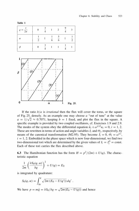
Chapter 6: Stability and Chaos 523
Table 1
= τ
2π0
3
41 2
9
43
α1
21
1
6
5
61
1
2
β 03
41 1
1
41
Fig. 25.
If the ratio b/a is irrational then the flux will cover the torus, or the squareof Fig. 25, densely. As an example one may choose a “out of tune” at the valuea = 1/
√2 ≈ 0.7071, keeping b = 1 fixed, and plot the flux in the square. A
specific example is provided by two coupled oscillators, cf. Exercises 1.9 and 2.9.The modes of the system obey the differential equation ui+ω(i)2ui = 0, i = 1, 2.These are rewritten in terms of action and angle variables Ii andΘi , respectively, bymeans of the canonical transformation (M2.95). They become Ii = 0, Θi = ω(i),i = 1, 2. Embedded in the phase space which is now four-dimensional, we find twotwo-dimensional tori which are determined by the given values of Ii = I 0
i = const.Each of these tori carries the flux described above.
6.3 The Hamiltonian function has the form H = p2/(2m)+ U(q). The charac-teristic equation
1
2m
(∂S0(q, α)
∂q
)2
+ U(q) = E0
is integrated by quadrature:
S0(q, α) =∫ q
q0
√2m(E0 − U(q ′)) dq ′ .
We have p = mq = ∂S0/∂q = √2m(E0 − U(q)) and hence
524 Solution of Exercises
t (q)− t (q0) =∫ q
q0
m√2m(E0 − U(q ′))
dq ′ = ∂S0
∂E0.
(This holds away from equilibrium positions, in case the system possesses anyequilibria.) Choose P ≡ α = E0. Then Q = ∂S0/∂E0 = t − t0, or, alternatively,(P = 0, Q = 1). Thus, we have achieved rectification of the Hamiltonian vectorfield: In the coordinates (P,Q) the particle moves on the straight line P = E0with velocity Q = 1.
Consider now an energy in the vicinity of E0, E = βE0, with β not farfrom 1. Let the particle travel from q0 to a point q ′ in such a way that the timet (q ′) − t (q0) is the same as for E0. Of course, p′0 =
√2m(E − U(q0)), and
p′ = √2m(E − U(q ′)), and
t − t0 =∫ q
q0
mdx√2m(E − U(x)) .
The new momentum is chosen to be P = E0 (the energy of the first orbit). Thenone has
Q = ∂S(q,E)∂E0
= β ∂S(q,E)∂E
= β(t − t0) ,
i.e., (P = 0, Q = β). In the new coordinates the particle again moves along thestraight line P = E0, this time, however, with velocity β. The particles on theorbits to be compared move apart linearly in time. If U(q) is such that in someregion of phase space all orbits are periodic, one should transform to action andangle variables, I (E) = const., Θ = ω(E)t +Θ0. Also in this situation one seesthat the orbits separate at most linearly in time. In the case of the oscillator, whereω is independent of E or I , their distance remains constant.
The integration described above is possible only if E is larger than the maxi-mum of U(q). For E = Umax(q) the running time goes to infinity logarithmically(cf. Sect. M1.23). The statement of this exercise does not apply when one of thetrajectories is a separatrix.
6.4 For µ = 0 the system becomes q1 = ∂H/∂q2 and q2 = −∂H/∂q1, withH = −λ(q2
1+q22 )/2+(q1q
22−q3
1/3)/2. The critical points (where the Hamiltonianvector field vanishes) are obtained from the system of equations −λq2+q1q2 = 0,λq1+ (q2
1 −q22 )/2 = 0. One finds the following solutions: P0 = (q1 = 0, q2 = 0),
P1/2 = (q1 = λ, q2 = ±√
3 λ), P3 = (q1 = −2λ, q2 = 0). Linearization in theneighborhood of P0 leads to q1 ≈ −λq2, q2 ≈ λq1. Thus P0 is a center. Lineariza-tion in the neighborhood of P1 is achieved by the transformation u1 := q1 − λ,u2 := q2 −
√3 λ, whereby the differential equations become.
u1 =√
3 λu1 + u1u2 ≈√
3 λu1 ;u2 = 2λu1 −
√3 λu2 +
(u2
1 − u22
)/2 ≈ 2λu1 −
√3 λu2 .
Chapter 6: Stability and Chaos 525
The flux tends to P1 along u1 = 0 but tends away from it along u2 = 0. Thus P1is a saddle point. The same is true for P2 and P3. One easily verifies that thesethree points belong to the same energy E = H(Pi) = −2λ3/3 and that they arepairwise connected by separatrices. Indeed, the straight lines q2 = ±(q1+2λ)/
√3
and q1 = λ are curves with constant energy E = −2λ3/3 and build up the triangle(P1, P2, P3).
If one switches on the damping terms by means of 1 µ > 0, P0 is still anequilibrium point because in the neighborhood of (q1 = 0, q2 = 0) we have(
q1q2
)≈
(−µ −λλ −µ
)(q1q2
)≡ A
(q1q2
).
From the equation det(x1l − A) = 0 one finds the characteristic exponents to bex1/2 = −µ ± iλ. Thus P0 becomes a node (a sink). The points P1, P2, and P3,however, are no longer equilibrium positions. The lines which connect them arebroken up.
6.5 We write H in two equivalent forms
(i) H = I1 + I2 with I1 =(p2
1 + q21
)/2+ q3
1/3 ,
I2 =(p2
2 + q22
)/2− q3
2/3 ,
(ii) H =(p2
1 + p22
)/2+ U(q1, q2) with U =
(q2
1 + q22
)/2+
(q3
1 − q32
)/3
=(Σ2 +∆2
)/4+Σ2∆/4+∆3/12 ,
where Σ := q1 + q2 , ∆ := q1 − q2 .
Then the equations of motion are
q1 = p1 , q2 = p2 ,
p1 = −q1 − q21 , p2 = −q2 + q2
2 .
The critical points of this system are P0 : (q1 = 0, q2 = 0, p1 = 0, p2 = 0),P1 : (0, 1, 0, 0), P2 : (−1, 0, 0, 0), P3 : (−1, 1, 0, 0). One easily verifies thatdIi/dt = 0, i = 1, 2, i.e., I1 and I2 are independent integrals of the motion. Thepoints P1 and P2 lie on two equipotential lines, viz. the straight line q1−q2 = −1,and the ellipse 3(q1+q2)
2+(q1−q2)2+2(q1−q2)−2 = 0. In either case U = 1/6.
As an example and using these results, one may sketch the projection of the fluxonto the plane (q1, q2).
6.6 The critical points of the system q = p, p = q−q3−p are P0 : (q = 0, p =0), P1 : (1, 0), and P2 = (−1, 0). Linearization around P0 gives
526 Solution of Exercises(q
p
)≈
(1 10 −1
)(q
p
)= A
(q
p
).
The eigenvalue of A are λ1/2 = (−1 ±√5)/2, hence λ1 > 0 and λ2 < 0 whichmeans that P0 is a saddle point. Linearizing in the neighborhood of P1 and intro-ducing the variables u := q − 1, v := p, the system becomes(
u
v
)≈
(0 1−2 −1
)(u
v
).
The characteristic exponents are µ1/2 = (−1± i√
7)/2. The same values are foundfor the system linearized in the neighborhood of P2. This means that both P1 andP2 are sinks.
The Liapunov function V (q, p) has the value 0 in P0, and the value −1/4in P1 and P2. One easily verifies that P1 and P2 are minima and that V in-creases monotonically in a neighborhood of these points. For instance, close toP1 take u := q − 1, v := p. Then Φ1(u, v) := V (q = u + 1, p = v) + 1/4 =v2/2 + u2 + u3 + u4/4. Indeed, at the point P1 we find Φ1(0, 0) = 0 while Φ1is positive in a neighborhood of P1.
Along solutions the function V (q, p), or, equivalently, Φ1(u, v), decreasesmonotonically. Let us check this for V :
dV
dt= dV∂pp + ∂V
∂qq = ∂V
∂p(q − q3 − p)+ ∂V
∂qp = −p2 .
In order to find out towards which of the two sinks a given initial configurationwill tend, one has to calculate the two separatrices that end in P0. They form theboundaries of the basins of P1 and P2 as indicated in Fig. 26 by the blank anddotted areas, respectively.
6.7 As x0, by assumption, is an isolated minimum, a Liapunov function is chosenas follows: V (x) := U(x) − U(x0). In a certain neighborhood M of x0, V (x) ispositive semi-definite and we have
d
dtV (x
˜) =
n∑i=1
∂V
∂xixi = −
n∑i=1
(∂U
∂xi
)2
.
If we follow a solution in the domain M\x0, V (x) decreases, i.e., all solutioncurves tend “inwards”, towards x0. Thus, this point is asymptotically stable.
In the example U(x1, x2) = x21 (x1 − 1)2 + x2
2 . The points x0 = (0, 0) andx′0 = (1, 0) are isolated minima and, hence, are asymptotically stable equilibria.
6.8 This system is Hamiltonian. A Hamiltonian function is H = p2/2+ q(q2 −3)/6. The phase portraits are obtained by drawing the curves H(q, p) = E =const. The Hamiltonian vector field vH = (p, (1− q2)/2) has two critical pointswhose nature is easily identified by linearizing in their neighborhoods. One finds
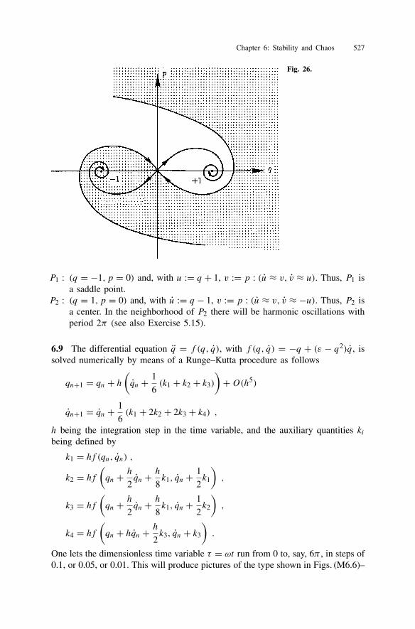
Chapter 6: Stability and Chaos 527
Fig. 26.
P1 : (q = −1, p = 0) and, with u := q + 1, v := p : (u ≈ v, v ≈ u). Thus, P1 isa saddle point.
P2 : (q = 1, p = 0) and, with u := q − 1, v := p : (u ≈ v, v ≈ −u). Thus, P2 isa center. In the neighborhood of P2 there will be harmonic oscillations withperiod 2π (see also Exercise 5.15).
6.9 The differential equation q = f (q, q), with f (q, q) = −q + (ε − q2)q, issolved numerically by means of a Runge–Kutta procedure as follows
qn+1 = qn + h(qn + 1
6(k1 + k2 + k3)
)+O(h5)
qn+1 = qn + 1
6(k1 + 2k2 + 2k3 + k4) ,
h being the integration step in the time variable, and the auxiliary quantities kibeing defined by
k1 = hf (qn, qn) ,k2 = hf
(qn + h
2qn + h
8k1, qn + 1
2k1
),
k3 = hf(qn + h
2qn + h
8k1, qn + 1
2k2
),
k4 = hf(qn + hqn + h
2k3, qn + k3
).
One lets the dimensionless time variable τ = ωt run from 0 to, say, 6π , in steps of0.1, or 0.05, or 0.01. This will produce pictures of the type shown in Figs. (M6.6)–
528 Solution of Exercises
(M6.8). Alternatively, one may follow the generation of these figures on the screenof a PC. One will notice that all of them tend quickly to the attractor.
6.10 The program developed in Exercise 6.9 may be used to print out, for a giveninitial configuration, the time τ and the distance from the origin d, each time theorbit crosses the line p = q. One finds the following result:
p = q > 0 :τ 5.46 11.87 18.26 24.54 30.80 37.13 43.47
d 0.034 0.121 0.414 1.018 1.334 1.375 1.378
p = q < 0 :τ 2.25 8.86 15.07 21.42 27.66 33.96 40.30
d 0.018 0.064 0.227 0.701 1.238 1.366 1.378
Plotting ln d versus τ shows that this function increases approximately linearly(with slope ≈ 0.1) until it has reached the attractor. Thus, the point of intersectionof the orbit and the straight line p = q wanders towards the attractor at an ap-proximately exponential rate. One finds a similar result for orbits which approachthe attractor from the outside.
6.11 The motion manifold of this system is R2. For the linearized system (x1 =x1, x2 = −x2) the straight line Ustab = (x1 = 0, x2) is a stable submanifold.Indeed, the velocity field points towards the equilibrium point (0, 0) and the char-acteristic exponent is −1. The straight line Uunst = (x1, x2 = 0), in turn, is anunstable submanifold: The velocity field points away from (0, 0) and the charac-teristic exponent is +1. The full system can be transformed to
x2 − x2 − 2x2 = 0 , x21 = x2 + x2 ,
whose general solution is
x2(t) = a exp(2t)+ b exp(−t) , x1(t) =√
3a exp t ,
or, equivalently,
x2 = 1
3x2
1 + b√
3a1
x1≡ 1
3x2
1 +c
x1.
Among this set of solutions the orbit with c = 0 goes through the point (0,0) andis tangent to Uunst in that point. On the submanifold Vunst = (x1, x2 = x2
1/3) thevelocity field moves away from (0, 0).
The corresponding stable submanifold of the full system coincides with Ustabbecause, with a = 0, x1(t) = 0, x2(t) = b exp(−t) which means that Vstab =(x1 = 0, x2).
6.12 We have xn+1 = 1 − 2x2n and yi = 4/π arcsin
√(xi + 1)/2 − 1. With
−1 ≤ xi ≤ 0 also −1 ≤ yi ≤ 0, and with 0 ≤ xi ≤ 1 also 0 ≤ yi ≤ 1. We
Chapter 6: Stability and Chaos 529
wish to know the relation between yn+1 and yn. First, the relation xn → yn+1 isyn+1 = 4/π arcsin(1−x2
n)1/2−1. Using the addition theorem arcsin u+arcsin v =
arcsin(u√
1− v2 + v√1− u2) and setting u = v = (1+ x)/2 one shows
arcsin√
1− x2 = 2 arcsin
√x + 1
2for − 1 ≤ x ≤ 0 ,
arcsin√
1− x2 = π − 2 arcsin
√x + 1
2for 0 ≤ x ≤ 1 .
In the first case yn ≤ 0 and yn+1 = 1+2yn, in the second case yn ≥ 0 and yn+1 =1−2yn. These can be combined to yn+1 = 1−2|yn|. The derivative of this iterativemapping is ±2; its magnitude is larger than 1. There are no stable fixed points.
6.15 If, for instance, m = 1, then zσ := exp(i2πσ/n) are the roots of the equationzn−1 = (z−z1) . . . (z−zn) = 0. They lie on the unit circle in the complex planeand neighboring roots are separated by the angle 2π/n. Expanding the product(z− z1) . . . (z− zn) = zn− z∑n
σ=1 zσ + . . . , one sees that, indeed,∑nσ=1 zσ = 0.
For the values m = 2, . . . , n− 1 we renumber the roots and obtain the same re-sult. For m = 0 and for m = n, however, the sum is equal to 0. Multiplyingxσ = ∑n
τ=1 xτ exp(−2iπστ/n)/√n by 1/
√n exp(2iπσλ/n) and summing over
σ one obtains
1√n
n∑σ=1
xσ e2iπσλ/n = 1
n
n∑τ=1
xτ
n∑σ=1
e2iπσ(τ−λ)/n =n∑τ=1
xτ δτλ = xλ .
This is used to calculate
gλ = 1
n
n∑σ=1
xσ xσ+λ = 1
n2
∑µ,ν
xµx∗n−ν
∑σ
e2iπ/n(σ(µ+ν)+λν) .
The orthogonality relation implies µ+ν = 0 (mod n), and we have used x∗n−ν = xν .Furthermore, xµ mod n = xµ and, finally, xµ and xn−µ have the same modulus.It follows that gλ = 1/n
∑nµ=1 |xµ|2 cos(2πλµ/n). The inverse of this formula
|xσ |2 =∑nλ=1 gλ cos(2πσλ/n) is obtained in the same way.
6.16 If we set y = αx + β, i.e., x = y/α − β/α, the relation
xi+1 = µxi(1− xi) = µ(
1
αyi − β
α
)(1+ β
α− 1
αyi
)will take the desired form provided α and β are chosen such that they fulfill theequations α + 2β = 0, β(1 − µ(α + β)/α) = 1. These give α = 4/(µ − 2),β = −α/2, and, therefore, γ = µ(µ− 2)/4. From 0 ≤ µ < 4 follows 0 ≤ γ < 2.One then sees easily that yi ∈ [−1,+1] is mapped onto yi+1 in the same inter-val. Let h(y, γ ) := 1 − γy2. The first bifurcation occurs when h(y, γ ) = y and∂h(y, γ )/∂y = 1, i.e., when γ0 = 3/4, y0 = 2/3, or, correspondingly, µ0 = 3/4,
530 Solution of Exercises
x0 = 2/3. Take then k := h h, i.e., k(y, γ ) = 1− γ (1− γy2)2. The second bi-furcation occurs at γ1 = 5/4. The corresponding value y1 of y is calculated fromthe system
k
(y,
5
4
)= −1
4+ 25
8y2 − 125
64y4 = y , (1)
∂k
∂y
(y,
5
4
)= 25
4y
(1− 5
4y2)= −1 . (2)
Combining these equations according to y · (2)–4 · (1), one finds the quadraticequation
y2 − 4
5y − 4
25= 0 ,
whose solutions are y1/2 = 2(1±√2)/5. From γ1 = 5/4 we have µ1 = 1+√6,from this and from y1/2, finally
x1/2 = 1
10
(4+√6± (
2√
3−√2)) = 0.8499 and 0.4400 .
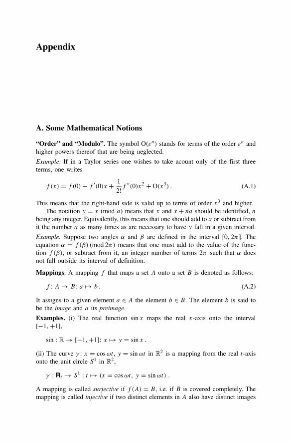
Appendix
A. Some Mathematical Notions
“Order” and “Modulo”. The symbol O(εn) stands for terms of the order εn andhigher powers thereof that are being neglected.
Example. If in a Taylor series one wishes to take acount only of the first threeterms, one writes
f (x) = f (0)+ f ′(0)x + 1
2!f′′(0)x2 + O(x3) . (A.1)
This means that the right-hand side is valid up to terms of order x3 and higher.The notation y = x (mod a) means that x and x + na should be identified, n
being any integer. Equivalently, this means that one should add to x or subtract fromit the number a as many times as are necessary to have y fall in a given interval.
Example. Suppose two angles α and β are defined in the interval [0, 2π ]. Theequation α = f (β) (mod 2π) means that one must add to the value of the func-tion f (β), or subtract from it, an integer number of terms 2π such that α doesnot fall outside its interval of definition.
Mappings. A mapping f that maps a set A onto a set B is denoted as follows:
f : A→ B: a → b . (A.2)
It assigns to a given element a ∈ A the element b ∈ B. The element b is said tobe the image and a its preimage.
Examples. (i) The real function sin x maps the real x-axis onto the interval[−1,+1],
sin : R → [−1,+1]: x → y = sin x .
(ii) The curve γ : x = cosωt , y = sinωt in R2 is a mapping from the real t-axisonto the unit circle S1 in R2,
γ : Rt → S1 : t → (x = cosωt, y = sinωt) .
A mapping is called surjective if f (A) = B, i.e. if B is covered completely. Themapping is called injective if two distinct elements in A also have distinct images
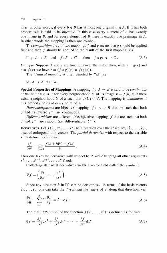
532 Appendix
in B, in other words, if every b ∈ B has at most one original a ∈ A. If it has bothproperties it is said to be bijective. In this case every element of A has exactlyone image in B, and for every element of B there is exactly one preimage in A.In other words the mapping is then one-to-one.
The composition f g of two mappings f and g means that g should be appliedfirst and then f should be applied to the result of the first mapping, viz.
If g: A→ B and f : B → C , then f g: A→ C . (A.3)
Example. Suppose f and g are functions over the reals. Then, with y = g(x) andz = f (y) we have z = (f g)(x) = f (g(x)).
The identical mapping is often denoted by “id”, i.e.
id: A→ A: a → a .
Special Properties of Mappings. A mapping f : A→ B is said to be continuousat the point u ∈ A if for every neighborhood V of its image v = f (u) ∈ B thereexists a neighborhood U of u such that f (U) ⊂ V . The mapping is continuous ifthis property holds at every point of A.
Homeomorphisms are bijective mappings f : A→ B that are such that bothf and its inverse f−1 are continuous.
Diffeomorphisms are differentiable, bijective mappings f that are such that bothf and f−1 are smooth (i.e. differentiable, C∞).
Derivatives. Let f (x1, x2, . . . , xn) be a function over the space Rn, e1, . . . , en,a set of orthogonal unit vectors. The partial derivative with respect to the variablexi is defined as follows:
∂f
∂xi= limh→0
f (x + hei )− f (x)h
. (A.4)
Thus one takes the derivative with respect to xi while keeping all other argumentsx1, . . . , xi−1, xi+1, . . . , xn fixed.
Collecting all partial derivatives yields a vector field called the gradient,
∇f =(∂f
∂x1, . . . ,
∂f
∂xn
). (A.5)
Since any direction n in Rn can be decomposed in terms of the basis vectorse1, . . . , en, one can take the directional derivative of f along that direction, viz.
∂f
∂n=
n∑i=1
ni∂f
∂xi≡ n · ∇f . (A.6)
The total differential of the function f (x1, . . . , xn) is defined as follows:
df = ∂f
∂x1dx1 + ∂f
∂x2dx2 + · · · + ∂f
∂xndxn . (A.7)
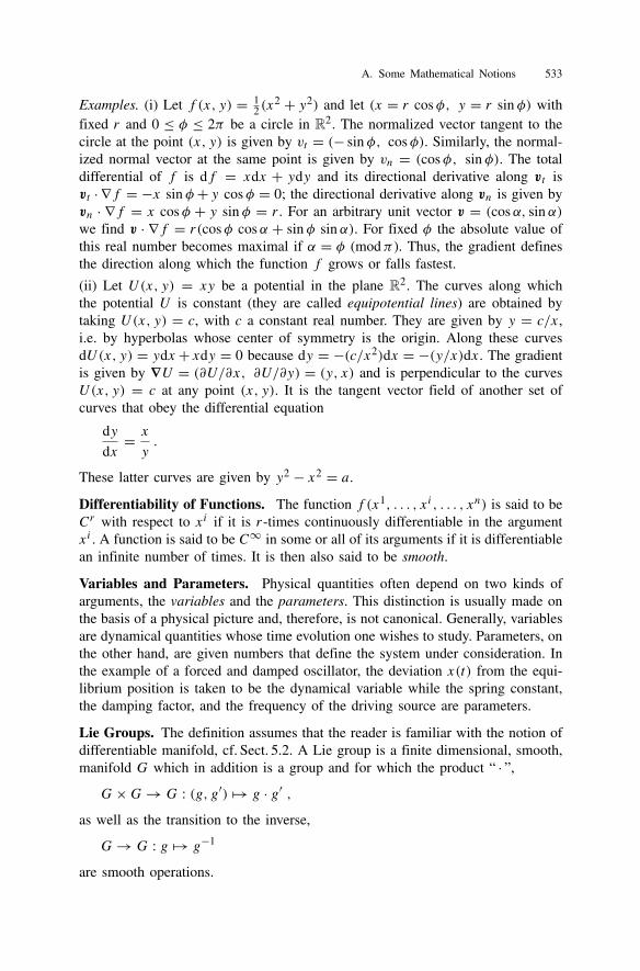
A. Some Mathematical Notions 533
Examples. (i) Let f (x, y) = 12 (x
2 + y2) and let (x = r cosφ, y = r sin φ) withfixed r and 0 ≤ φ ≤ 2π be a circle in R2. The normalized vector tangent to thecircle at the point (x, y) is given by vt = (− sin φ, cosφ). Similarly, the normal-ized normal vector at the same point is given by vn = (cosφ, sin φ). The totaldifferential of f is df = xdx + ydy and its directional derivative along vt isvt · ∇f = −x sin φ+ y cosφ = 0; the directional derivative along vn is given byvn · ∇f = x cosφ + y sin φ = r . For an arbitrary unit vector v = (cosα, sin α)we find v · ∇f = r(cosφ cosα + sin φ sin α). For fixed φ the absolute value ofthis real number becomes maximal if α = φ (modπ ). Thus, the gradient definesthe direction along which the function f grows or falls fastest.
(ii) Let U(x, y) = xy be a potential in the plane R2. The curves along whichthe potential U is constant (they are called equipotential lines) are obtained bytaking U(x, y) = c, with c a constant real number. They are given by y = c/x,i.e. by hyperbolas whose center of symmetry is the origin. Along these curvesdU(x, y) = ydx+ xdy = 0 because dy = −(c/x2)dx = −(y/x)dx. The gradientis given by ∇U = (∂U/∂x, ∂U/∂y) = (y, x) and is perpendicular to the curvesU(x, y) = c at any point (x, y). It is the tangent vector field of another set ofcurves that obey the differential equation
dy
dx= xy.
These latter curves are given by y2 − x2 = a.
Differentiability of Functions. The function f (x1, . . . , xi, . . . , xn) is said to beCr with respect to xi if it is r-times continuously differentiable in the argumentxi . A function is said to be C∞ in some or all of its arguments if it is differentiablean infinite number of times. It is then also said to be smooth.
Variables and Parameters. Physical quantities often depend on two kinds ofarguments, the variables and the parameters. This distinction is usually made onthe basis of a physical picture and, therefore, is not canonical. Generally, variablesare dynamical quantities whose time evolution one wishes to study. Parameters, onthe other hand, are given numbers that define the system under consideration. Inthe example of a forced and damped oscillator, the deviation x(t) from the equi-librium position is taken to be the dynamical variable while the spring constant,the damping factor, and the frequency of the driving source are parameters.
Lie Groups. The definition assumes that the reader is familiar with the notion ofdifferentiable manifold, cf. Sect. 5.2. A Lie group is a finite dimensional, smooth,manifold G which in addition is a group and for which the product “ · ”,
G×G→ G : (g, g′) → g · g′ ,as well as the transition to the inverse,
G→ G : g → g−1
are smooth operations.
534 Appendix
G being a group means that it fulfills the group axioms, cf. e.g., Sect. 1.13:There exists an associative product; G contains the unit element e; for every g ∈ Gthere exists an inverse g−1 ∈ G. Loosely speaking, smoothness means that thegroup elements depend differentiably on parameters, which may be thought of asangles for instance, and that group elements can be deformed in a continuous anddifferentiable manner.
A simple example is the unitary group
U(1) =
eiα|α ∈ [0, 2π ].
This is an Abelian group (i.e., a commutative group). Further examples areprovided by the rotation group SO(3) in three real dimensions, and the unitarygroup SU(2) which are dealt with in Sects. 2.21 and 5.2.3 (iv). The Galilei groupis defined in Sect. 1.13, the Lorentz group is discussed in Sects. 4.4 and 4.5.
B. Historical Notes
There follow some biographical notes on scientists who made important contribu-tions to mechanics. Without striving for completeness, the founders of mechanicsproper are marked by an asterisk and are treated in somewhat more detail.
∗d’Alembert, Jean-Baptiste: born 17 November 1717 in Paris, died 29 October1783 in Paris. Writer, philosopher, and mathematician. Co-founder of the Ency-clopédie. Important contributions to mathematics, mathematical physics and as-tronomy. His principal work “Traité de dynamique” contains the principle whichbears his name.
Arnol’d, Vladimir Igorevich: 1936– , Russian mathematician.
Cartan, Elie: 1869–1951, French mathematician.
Coriolis, Gustave-Gaspard: 1792–1843, French mathematician.
Coulomb, Charles Augustin: 1736–1806, French physicist.
∗Descartes, René (Cartesius): born 31 March 1596 in La Haye (Touraine), died11 February 1650 in Stockholm. French philosopher, mathematician and naturalphilosopher. In spite of the fact that Descartes’ contributions to mechanics were nottoo successful (for instance, he proposed incorrect laws of collision), he contributeddecisively to the development of analytic thinking without which modern naturalscience would not be possible. In this regard his book Discours de la Méthodepour bien conduire sa Raison, published in 1637, was particularly important. Alsohis imaginative conceptions – ether whirls carrying the planets around the sun;God having given eternal motion to the atoms relative to the atoms of the etherwhich span our space; the state of motion of atoms being able to change only
A. Some Mathematical Notions 535
by collisions – inspired the amateur researchers of the 17th century considerably.It was in this community where the real scholars of science found the resonanceand support which they did not obtain from the scholastic and rigid attitude of theuniversities of their time.
∗Einstein, Albert: born 14 March 1879 in Ulm (Germany), died 18 April 1955 inPrinceton, N.J. (U.S.A.). German-Swiss physicist, 1940 naturalized in the U.S.A.His most important contribution to mechanics is Special Relativity which he pub-lished between 1905 and 1907. In his General Relativity, published between 1914and 1916, he succeeded in establishing a (classical) description of gravitation asone of the fundamental interactions. While Special Relativity is based on the as-sumption that space-time is the flat space R4, General Relativity is a dynamicaland geometric field theory which allows one to determine the metric on space-timefrom the sources, i.e., from the given distribution of masses in the universe.
∗Euler, Leonhard: born 15 April 1707 in Basel (Switzerland), died 18 September1783 in St. Petersburg (Russia). Swiss mathematician. Professor initially of physics,then of mathematics at the Academy of Sciences in St. Petersburg (from 1730 until1741, and again from 1766 onwards), and, at the invitation of Frederick the Great,member of the Berlin Academy (1741–1766). Among his gigantic scientific workparticularly relevant for mechanics: development of variational calculus; law ofconservation of angular momentum as an independent principle; equations of mo-tion for the top. He also made numerous contributions to continuum mechanics.
Fibonacci, Leonardi: ∼1120–∼1240. Italian mathematician who introduced theIndian-Arabic system of numbers. See also Fibonacci numbers in Sect. 6.5.
∗Galilei, Galileo: born 15 February 1564 in Pisa (Italy), died 8 January 1642in Arcetri near Florence (Italy). Italian mathematician, natural philosopher, andphilosopher, who belongs to the founding-fathers of natural sciences in the mod-ern sense. Professor in Pisa (1589–1592), in Padua (1592–1610), mathematicianand physicist at the court of the duke of Florence (1610–1633). From 1633 on un-der confinement to his house in Arcetri, as a consequence of the conflict with PopeUrban VIII and the Inquisition, which was caused by his defence of the Coper-nican, heliocentric, planetary system. Galilei made important contributions to themechanics of simple machines and to observational astronomy. He developed thelaws of free fall.
∗Hamilton, William Rowan: born 4 August 1805 in Dublin (Ireland), died 2September 1865 in Dunsink near Dublin. Irish mathematician, physicist, and as-tronomer. At barely 22 years of age he became professor at the university of Dublin.Important contributions to optics and to dynamics. Developed the variational prin-ciple which was cast in its later and more elegant form by C.G.J. Jacobi.
∗Huygens, Christiaan: born 14 April 1629 in The Hague (Netherlands), died 8July 1695 in The Hague. Dutch mathematician, physicist and astronomer. From
536 Appendix
1666 until 1681 member of the Academy of Sciences in Paris. Although Huygensis not mentioned explicitly in this book he made essential contributions to me-chanics: among others the correct laws for elastic, central collisions and, buildingon Galilei’s discoveries, the classical principle of relativity.
Jacobi, Carl Gustav Jakob: 1804–1851, German mathematician.
∗Kepler, Johannes: born 27 December 1571 in Weil der Stadt (Germany), died15 November 1630 in Regensburg (Germany). German astronomer and mathemati-cian. Led a restless live, in part due to numerous misfortunes during the turbulenttimes before and during the Thirty Years War, but also for reasons to be found inhis character. Of greatest importance for him was his acquaintance with the Danishastronomer Tyge (Tycho) Brahe, in the year 1600 in Prague, whose astronomicaldata were the basis for Kepler’s most important works. Succeeding T. Brahe, Ke-pler became mathematician and astrologer at the imperial court, first under emperorRudolf II, later under Mathias. Finally, from 1628 until his death in 1630, he wasastrologer of the duke of Friedland and Sagan, A. von Wallenstein. Kepler’s firsttwo laws are contained in his Astronomia nova (1609), the third is contained inhis main work Harmonices Mundi (1619). They were not generally accepted, how-ever, until Newton’s work who gave them a new, purely mechanical foundation.Kepler’s essential achievement was to overcome the ancient opposition betweencelestial mechanics (where the circle was believed to be the natural inertial typeof movement) on one hand and terrestial mechanics on the other.
Kolmogorov, Andrei Nikolaevic: 1903–1987, Russian mathematician.
∗Lagrange, Joseph Louis: born 25 January 1736 in Torino, died 10 April 1813in Paris. Italian-French mathematician. At the early age of 19 professor for mathe-matics at the Royal School of Artillery in Torino, from 1766 member of the BerlinAcademy, succeeding d’Alembert, then from 1786 member of the French Academyof Sciences, professor at Ecole Normale, Paris, in 1795 and at Ecole Polytechniquein 1797. His major work Mécanique Analytique which appeared in 1788, afterNewton’s Principia (1688) and Euler’s Mechanica (1736), is the third of the his-torically important treatises of mechanics. Of special relevance for mechanics werehis completion of variational calculus which he used to derive the Euler-Lagrangeequations of motion, and his contributions to celestial perturbation theory.
∗Laplace, Pierre Simon de: born 28 March 1749 in Beaumont-en-Auge(France), died 5 March 1827 in Paris. French mathematician and physicist. From1785 on member of the Academy, he became professor for mathematics at EcoleNormale (Paris) in 1794. He must have been rather flexible because he survivedfour political systems without harm. Under Napoleon he was for a short time Sec-retary of the Interior. Besides important contributions to celestial mechanics onthe basis of which the stability of the planetary system was rendered plausible, hedeveloped potential theory, along with Gauß and Poisson. Other important publi-cations of his deal with the physics of vibrations and with thermodynamics.
A. Some Mathematical Notions 537
Legendre, Adrien Marie: 1752–1833, French mathematician.
Leibniz, Gottfried Wilhelm: 1646–1716, German natural philosopher and phi-losopher.
Lie, Marius Sophus: 1842–1899, Norwegian mathematician.
Liapunov, Aleksandr Mikhailovich: 1857–1918, Russian mathematician.
Liouville, Joseph: 1809–1882, French mathematician.
Lorentz, Hendrik Antoon: 1853–1928, Dutch physicist.
∗Maupertuis, Pierre Louis Moreau de: born 28 September 1698 in St. Malo(Britanny, France), died 27 July 1759 in Basel (Switzerland). French mathemati-cian and natural philosopher. From 1731 paid member of the Academy of Sci-ences of France, in 1746 he became the first president of the Prussian AcadémieRoyale des Sciences et Belles Lettres, newly founded by Frederick the Great inBerlin who called many important scientists to the academy, notably L. Euler. In1756, seriously ill, Maupertuis returned first to France but then joined his friendJoh. II Bernoulli in Basel where he died in 1759. Along with Voltaire, Mauper-tuis was a supporter of Newton’s theory of gravitation which he had come toknow while visiting London in 1728, and fought against Descartes’ ether whirls.Of decisive importance for the development of mechanics was his principle ofleast action, formulated in 1747, although his own formulation was still some-what vague (the principle was formulated in precise form by Euler and Lagrange).A widely noticed dispute of priority started by the Swiss mathematician SamuelKönig who attributed the principle to Leibniz, was eventually decided in favorof Maupertuis. This dispute alienated Maupertuis from the Prussian Academy andcontributed much to his bad state of health.
Minkowski, Hermann: 1864–1909, German mathematician.
Moser, Jürgen: 1928–1999, German mathematician.
∗Newton, Isaac: born 24 December 1642 in Whoolsthorpe (Lincolnshire, Eng-land), died 20 March 1726 in Kensington (London), (both dates according to theJulian calender which was used in England until 1752). Newton, who had studiedtheology at Trinity College Cambridge, learnt mathematics and natural sciencesessentially by himself. His first great discoveries, differential calculus, dispersionof light, and the law of gravity which he communicated to a small circle of expertsin 1669, so impressed Isaac Barrow, then holding the “Lucasian Chair” of mathe-matics at Trinity College, that he renounced his chair in favor of Newton. In 1696Newton was called at the Royal Mint and became its director in 1699. The RoyalSociety of London elected him president in 1703. Venerated and admired as thegreatest English natural philosopher, Newton was buried in Westminster Abbey.
His principal work, with regard to mechanics, is the three-volume PhilosophiaNaturalis Principia Mathematica (1687) which he wrote at the instigation of his
538 Appendix
pupil Halley and which was edited by Halley. Until this day the Principia havebeen studied and completely understood only by very few people. The reason forthis is that Newton’s presentation uses a highly geometrical language, divides mat-ters into “definitions” and “axioms” which mutually complete and explain one an-other, following examples from antiquity, in a manner difficult to understand forus, and because he presupposes notions of scholastic and Cartesian philosophy weare normally not familiar with. Even during Newton’s lifetime it took a long timebefore his contemporaries learned to appreciate this difficult and comprehensivework which, in addition to Newton’s laws, deals with a wealth of problems in me-chanics and celestial mechanics, and which contains Newton’s original ideas aboutspace and time that have stimulated our thinking ever since. Newton completed along development that began during antiquity and was initiated by astronomy, byshowing that celestial mechanics is determined only by the principle of inertia andthe gravitational force and, hence, that it follows the same laws as the mechanicsof our everyday world. At the same time he laid the foundation for a developmentwhich to this day is not concluded.
Noether, Emmy Amalie: 1882–1935, German mathematician. Belongs to thegreat scientific personalities in the mathematics of the 20th century.
∗Poincaré, Jules Henri: born 29 April 1854 in Nantes (France), died 17 July1912 in Paris. French mathematician, professor at Sorbonne university in Paris.Poincaré, very broad and extraordinarily productive, made important contributionsto the many-body problem in celestial mechanics for which he received a prizedonated by King Oscar II of Sweden. (Originally the prize was announced for theproblem of convergence of the celestial perturbation series, the famous problemof the “small denominators” that was solved much later by Kolmogorov, Arnol’d,and Moser.) Poincaré may be considered the founder of qualitative dynamics andof the modern theory of dynamical systems.
Poisson, Siméon Denis: 1781–1840, French mathematician.
Bibliography
Mechanics Textbooks and Exercise Books
Fetter, A.L., Walecka, J.D.: Theoretical Mechanics of Particles and Continua (McGraw Hill, NewYork 1980)
Goldstein, H.: Classical Mechanics (Addison-Wesley, Reading 1980)Honerkamp, J., Römer, H.: Theoretical Physics (Springer, Berlin, Heidelberg 1993)Landau, L.D., Lifshitz, E.M.: Mechanics (Pergamon, Oxford and Addison-Wesley, Reading 1971)Spiegel, M.R.: General Mechanics, Theory and Applications (McGraw Hill, New York 1976)
Some General Mathematical Texts
Arnol’d, V.I.: Ordinary Differential Equations (Springer, New York, Berlin, Heidelberg 1992)Arnol’d, V.I.: Geometrical Methods in the Theory of Ordinary Differential Equations (Springer, New
York, Berlin, Heidelberg 2nd ed. 1988)Flanders, H.: Differential Forms (Academic, New York 1963)Hamermesh, M.: Group Theory and Its Applications to Physical Problems (Addison-Wesley, Reading
1962)
Special Functions and Mathematical Formulae
Abramowitz, M., Stegun, I.A.: Handbook of Mathematical Functions (Dover, New York 1965)Gradshteyn, I.S., Ryzhik, I.M.: Tables of Integrals, Series and Products (Academic, New York 1965)
Chapter 2
Boccaletti, D., Pucacco, G.: Theory of Orbits 1+2 (Springer, Berlin, Heidelberg 1996, 1999)Rüssmann, H.: Konvergente Reihenentwicklungen in der Störungstheorie der Himmelsmechanik, Se-
lecta Mathematica V (Springer, Berlin, Heidelberg 1979)Rüssmann, H.: Non-degeneracy in the Perturbation Theory of Integrable Dynamical Systems, in Dod-
son, M.M., Vickers, J.A.G. (eds.) Number Theory and Dynamical Systems, London MathematicalSociety Lecture Note Series 134 (Cambridge University Press 1989)
Chapter 4
Ellis, G.F.R., Williams, R.M.: Flat and Curved Space-Times (Clarendon Press, Oxford, 1994)Hagedorn, R.: Relativistic Kinematics (Benjamin, New York 1963)Jackson, J.D.: Classical Electrodynamics (Wiley, New York 1975)Sexl, R.U., Urbantke, H.K.: Relativität, Gruppen, Teilchen (Springer, Berlin, Heidelberg 1976)Weinberg, S.: Gravitation and Cosmology, Principles and Applications of the General Theory of
Relativity (Wiley, New York 1972)
540 Bibliography
Chapter 5
Abraham, R., Marsden, J.E.: Foundations of Mechanics (Benjamin Cummings, Reading 1981)Arnol’d, V.I.: Mathematical Methods of Classical Mechanics (Springer, New York, Berlin, Heidelberg
2nd ed. 1989)Guillemin, V., Sternberg, S.: Symplectic Techniques in Physics (Cambridge University Press, New
York 1990)Hofer, H., Zehnder, E.: Symplectic Invariants and Hamiltonian Dynamics (Birkhäuser, Basel, 1994)Marsden, J.E., Ratiu, T.S.: Introduction to Mechanics and Symmetry (Springer, New York, 1994)O’Neill, B.: Semi-Riemannian Geometry, With Applications to Relativity (Academic, New York 1983)Thirring, W.: A Course in Mathematical Physics, Vol. 1: Classical Dynamical Systems (Springer,
Berlin, Heidelberg 2nd ed. 1992)
Chapter 6
Arnol’d, V.I.: Catastrophe Theory (Springer, Berlin, Heidelberg 1986)Bergé, P., Pomeau, Y., Vidal, C.: Order within Chaos; Towards a Deterministic Approach to Tur-
bulence (Wiley, New York 1986) French original (Hermann, Paris 1984)Chirikov, B.V.: A Universal Instability of Many-Dimensional Oscillator Systems, Physics Reports
52, 263 (1979)Collet, P., Eckmann, J.P.: Iterated Maps on the Interval as Dynamical Systems (Birkhäuser, Boston
1990)Devaney, R.L.: An Introduction to Chaotic Dynamical Systems (Benjamin Cummings, Reading 1989)Feigenbaum, M.: J. Stat. Phys. 19, 25 (1978) and 21, 669 (1979)Guckenheimer, J., Holmes, P.: Nonlinear Oscillations, Dynamical Systems, and Bifurcations of Vector
Fields (Springer, Berlin, Heidelberg 1990)Hénon, M., Heiles, C.: Astron. Journ. 69, 73 (1964)Hirsch, M.W., Smale, S.: Differential Equations, Dynamical Systems and Linear Algebra (Academic,
New York 1974)Palis, J., de Melo, W.: Geometric Theory of Dynamical Systems (Springer, Berlin, Heidelberg 1982)Peitgen, H.O., Richter, P.H.: The Beauty of Fractals, Images of Complex Dynamical Systems (Springer,
Berlin, Heidelberg 1986)Ruelle, D.: Chance and Chaos (Princeton University Press, New Jersey, 1991)Ruelle, D.: D.: Elements of Differential Dynamics and Bifurcation Theory (Academic, New York
1989)Schuster, H.G.: Deterministic Chaos, An Introduction (Physik-Verlag, Weinheim 1987)Wisdom, J.: Chaotic Behaviour in the Solar System, Nucl. Phys. B (Proc. Suppl.) 2, 391 (1987)
Author Index
Abraham, R. 321Arnol’d, V.I. 167, 171, 331, 352, 534
Beckmann, P. 400Bergé, P. 391Bernoulli, Joh.I 491Bertrand, J. 53
Cantor, G. 408Cartan, E. 534Collet, P. 391Coriolis, G.G. 54, 534Coulomb, Ch.A. 8, 534
D’Alembert, J.-B. 89, 534Darboux, G. 328Descartes, R.C. 534Devaney, R.L. 391
Ebenfeld, St. 231, 238Eckmann, J.P. 391Einstein, A. 8, 535Ellis, G.F.R. 279Euler, L. 76, 205, 535
Feigenbaum, M. 398Fermat, P. de 95Fibonacci, L. 404, 535
Galilei, Galileo 24, 239, 535Goldstein, H. 491Guckenheimer, J. 168, 379, 385Guillemin, V. 328
Hénon, M. 412Hamilton, W.R. 98, 149, 535Hausdorff, F. 287Heiles, C. 412Helmont, J.B. 393Hofer, H. 347Holmes, Ph. 168, 379, 385Hooke, R. 9
Huygens, C. 535
Jackson, J.D. 276Jacobi, C.G.J. 149, 450, 536
Kepler, J. 16, 18, 536Klavetter, J. 415Kolmogorov, A.N. 167, 536
Lagrange, J.L. 536Lagrange, P.-S. de 92Laplace, P.S. de 491, 536Legendre, A.M. 105, 537Leibniz, G.W. 537Lenz, H.F.E. 491Liapunov, A.M. 369, 537Lie, M.S. 537Liouville, J. 134, 160, 331, 537Lorentz, H.A. 244, 275, 537
Marsden, J.E. 321Maupertuis, P.L.M. de 537Minkowski, H. 537Moser, J. 167, 537
Newhouse, S. 395Newton, I. 1, 537Noether, E.A. 26, 113, 538
O’Neill, B. 299
Pauli, W. 260Poincaré, J.H. 250, 379, 538Poinsot, L. 219Poisson, S.D. 140, 538Pomeau, Y. 391Publius Ovidius Naso 393
Rüssmann, H. 168Ruelle, D. 395Runge, C. 491Rutherford, E. 70
542 Author Index
Scheck, F. 231, 238Shaw, R.S. 395Steiner, J. 196Sternberg, S. 328Stokes, G.G. 30Sussman, G.J. 165
Takens, F. 395
Thirring, W. 168
Vidal, C. 391
Williams, R.M. 279Wisdom, J. 165, 409
Zehnder, E. 347
Subject Index
Acceleration 4Action function 149Action integral 98Action variable 126Addition of velocities 262Adiabatic invariants 171Affine fibre bundle 267Angle variable 126Angular momentum of rigid body 201Angular velocity 221Anharmonic oscillator 168Aphelion 48Apocenter 48Asteroid belt 415Asymptotically stable 363Atlas 290Attractor 376
basin of 376Attractors 371Atwood’s machine 94Autonomous systems 112Averaging principle 168Axial vector 317
Base differential forms 306Base fields 302Base integral curve 343Bertrand’s theorem 53Bifurcation 372
codimension of 385Bifurcations of flows 384Body-fixed system 209Boosts 252Bundle
cotangent 305tangent 300
Canonical 108Canonical coordinates 328Canonical equations 108, 329Canonical one-form 322
Canonical transformations 121Canonical two-form 324Cantor set of the middle third 408Cartan derivative 313Center 365Center-of-mass 11Center-of-mass principle 23Central collision 66Characteristic equation of Hamiltonian and
Jacobi 150Characteristic exponents 362Charged particle in electric and magnetic fields
100Charged particle in electromagnetic fields 110Charts 286Christoffel symbols 349Classical field theory 432Closed n-particle system 23Commutator of vector fields 304Complete vector field 359Cone
light 249nutation 204space 204
Conformal group 282Connection 348Conservation
of angular momentum 23of Energy 23
Constantgravitational 10
Constraints 87Rheonomic 88scleronomic 88
constraints 88Contravariant 245Coordinate manifold 317Coordinate system
chart 289local 289
Countable basis 287
544 Subject Index
Coupled Van der Pol oscillators 378Covariant 104, 245, 270Covariant derivative 348, 349Curl 30Cyclic coordinates 105
D’Alembert’s principle 89Damped oscillator 373Darboux’s theorem 326Decay π → µ+ ν 455Decomposition theorem 257Degrees of freedom 37Deimos 410Derivative
directional 532partial 532
Deterministic 39Deterministic Chaos 390Diffeomorphisms 102, 532Differentiable dynamics 358Differentiable manifolds 287, 289Differential cross section 68Differential equationi of Hamilton and Jacobi
149Differential form 305Differential systems 39Dilatations 282Dissipative systems 355, 372Dynamical systems 356Dynamical variables 11, 419
Earth 217Effective potential 48Electric charges 8Elliptic integral of the first kind 45Energy 240
kinetic 273rest 273
Energy function 340Energy–momentum vector 272Equilibrium position 360Equipotential lines 533Equivalence principle 8Ergodic 167Euler’s differential equation of variational
calculus 97Euler’s equations 213, 214Euler’s equations of motion 211Euler–Lagrange equation for continuous
systems 425Euler–Lagrange equations 98, 344Eulerian angles 206Event 11
Extended phase space 40Extensive 7, 191Exterior
derivative 307, 313product 307, 311
Exterior product 311
Fermat’s principle 95Fibonacci numbers 404Fibres 300Fields 419Fitzgerald–Lorentz contraction 277Flow 39
fronts 359local 359maximal 359
Flux 359Force
central 13, 20centrifugal 55conservative 29Coriolis 55external 8, 20field 7frictional 234generalized 91gravitational 8harmonic 9internal 8, 20Lorentz 275of constraint 90
Form invariant 5, 270Fractals 407Frequency doubling 401Friction
gliding 230rolling 230rotational 230
Functionsmooth 288
Galilei grouporthochronous 25proper 25
Galilei invariant space-time 267Gauge transformations 101Generalized coordinates 89Generating function of canonical transformation
123Generating function of the infinitesimal
transformation 145Generator for infinitesimal rotations 115, 120Generators of boots 456Generators of rotations 456
Subject Index 545
Geodesic 347Geometric similarity 441Golden mean 404Gradient 532Gradient flow 382Gradient flows 461Group
axioms 26
Hénon’s attractor 462Hamilton function 104Hamilton’s principal function 452Hamilton’s variational principle 99Hamilton’s variational principle for continuous
systems 425Hamiltonian systems 330, 372Hamiltonian vector field 297, 330Harmonic oscillator 33, 157Hausdorff space 287Hermann–Bernoulli–Laplace vector 450Hodge star operation 316Hodge star operator 458Holonomic 87Homeomorphisms 532Hopf bifurcation 387Hyperion 410
Impact parameter 67Impact vector 67Inertia tensor 189, 191Inertial frames 5Infinitesimal canonical transformations 145Infinitesimal rotations 119Infinitesimally symplectic matrix 367Inhomogeneous Lorentz group 250Initial conditions 5, 38Inner product 332Integrable Systems 160Integrable systems 154Integral curve 38, 310Integrals of the motion 146Intermittency 401International System of Units (SI) 9Invariant plane 219Involution 159Iterative mappings on the unit interval 391
Jacobi identity 143Jacobian coordinates 450Jupiter 415
KAM theorem 167KAM tori 415Kepler problem 51, 441
Kepler’s first law 17Kepler’s Problem 13Kepler’s second law 16Kepler’s third law 18, 472Kinetic energy 189Kinetic energy of a rigid body 190Kirkwood gaps 409, 415Klein–Gordon equation 427
Lagrange’s equations 93Lagrangian function 93, 280Lagrangian multiplier 281Lagrangian two-form 339Lagrangian vector field 340Legendre transformation 105
geometrical interpretation 446Leibniz rule 298, 314, 348, 349Lenz’ vector 450Levi–Civita connection 349Liapunov characteristic exponents 401, 405Liapunov function 369Liapunov stable 363Lie
algebra 120derivative 331group 120, 533product 120
Lie bracket 459Lie derivative 304Lightlike 249Line element 270Linear autonomous systems 127Linear chain 420Linear systems 41Linearization in neighborhood of critical point
360Linearization in neighborhood of given solution
361Liouville’s theorem 135, 330Local coordinates 286Local rectification 154Local transverse section 380Logistic equation 396Lorentz invariant space-time 268
Manifold 284Mapping
bijective 532continuous 532injective 531regular 338surjective 531
Mappings of manifolds 307
546 Subject Index
Mars 415Mass
density 75electron 271gravitational 8inertial 6, 8reduced 12rest 271
Mass points 2Mass term 433Mathematical Pendulum 137Maximal integral curve 311, 359Metric 319
Riemannian 320semi-Riemannian 320
Metric tensor 245Minkowski space-time manifold 249Modulo 531Momentum 6, 240Momentum canonically conjugate to the
coordinate 105Motion 167Multipole moments 78Muon 242, 274
n-particle system 99Natural coordinate functions 288Neutrino 274Newton’s equation 270Noether’s theorem 113, 448Nonresonant torus 167Normal coordinates 182Nutation 227
One–form 305Orbital angular momentum 13Orthochronous 251Orthogonality relation 394
Parallel vector fields 350Parameter 419Parameters 11, 533Parity 27Particles 2Pauli matrix 260Pendulum chain 428Pericenter 48Perihelion 48
precession of 82Periodic orbits 388Perturbation theory 165Phase
portraits 33space 33
Phobos 410Photon 241π meson 241Pirouette 453Pitchfork bifurcation 387Planar mathematical pendulum 35, 183Platonic year 218Pluto 165, 417Poincaré group 250Poincaré mapping 381Poinsot’s construction 219Poisson bracket 140, 224, 281, 332Poisson’s theorem 144Potential 13Principal moments of inertia 192Principle
of center-of-mass motion 21Principle of Euler and Maupertuis 451Principle-axes systems 192Projectile 64, 455Projection 301Proper Lorentz transformations 250Proper orthochronous Lorentz group 252Proper time 3, 269Pull-back 308, 459Push-forward 308
Quasiperiodic Hamiltonian systems 164Quasiperiodic motion 403
Rn 288, 291
R-linearity 298Radioactive decay 242Rapidity 254Real symplectic group Sp2f (R) 131Rectification theorem 156Reduced action 150Regular precession 204Relative motion 12Resonant tori 167Rest energy 241Restricted three-body problem 164Reversal of motion 27Riemannian manifold 347Rigid body 185, 187Rod 187, 203Roessler’s model 462Rosettelike orbits 84Rotation group 117Routes to Chaos 401Runge–Kutta procedure 184, 527Rutherford scattering 70, 71, 85
Saddle-node bifurcation 386
Subject Index 547
Saturn 410Scale contraction 277Scattering orbits 84Secular perturbation 166Sine–Gordon equation 429Small oscillations 42, 180Smooth curve 296Smooth function on a manifold 296Smooth overlap 290Snowflake set 408SO(3) 117, 185, 294Soliton solutions 430Space
base 300cotangent 305homogeneous 3isotropic 3phase 317reflection 27velocity 317
Spacelike 249Special conformal transformations 282Special Lorentz boosts 253Special Lorentz transformations 253, 256Speed of light 243Spherical mathematical pendulum 162Spherical symmetry 2Spherical top with friction 229Spin
electron 456Stability
asymptotic 374Liapunov 374orbital 374
Steiner’s theorem 195Stokes’ theorem 30Strange attractors 371, 395, 407SU(2) 120, 293Symplectic
charts 328form 328geometry 328
Systemcenter-of-mass 65laboratory 65
Tangent vectors 298Target 64, 455Tensor field 319Tensor of field strengths 276Theorem of Kolmogorov, Arnol’d and Moser
167Time dilatation 277
Time reversal 27Time-dependent Hamiltonian systems 335Timelike 249Tippe top 229, 238Top
sleeping 226spherical 193, 203standing 227symmetric 193, 204, 215, 236symmetric children’s 225triaxial 193, 214
Torus 293Total angular momentum 23Total differential 532Total elastic cross section 70Transcritical bifurcation 386Transformation
affine 248Legendre 337scale 247
Uniform rectilinear motion 4Unitary unimodular group 293Units 10Universality of the speed of light 240
Van der Pol’s equation 377Variable
action 163angle 163
Variables 533Variational calculus 96Variational derivative 97Variational principles 95Vector field 302
complete 311Vector fields 38Velocity 4
angular 188translational 188
Vibrating string 420Virial 79Virial theorem 79Virtual displacement 89Voyager 1 and 2 missions 410
Wave equation 424Winding number 404World
events 243line 243points 243
World line 269

![Applications of Fractional Calculus to Newtonian Mechanics · PDF fileApplications of Fractional Calculus to Newtonian Mechanics Gabriele U. Varieschi ... In applied physics [5], FC](https://img.dokumen.tips/doc/110x75/5a78c7977f8b9aa17b8c696c/applications-of-fractional-calculus-to-newtonian-mechanics-of-fractional-calculus.jpg)


