Embed Size (px)
Citation preview

8/3/2019 Chap002 Modified
http://slidepdf.com/reader/full/chap002-modified 1/76

8/3/2019 Chap002 Modified
http://slidepdf.com/reader/full/chap002-modified 2/76
Chapter 2 (& 9)
Labor Supply

8/3/2019 Chap002 Modified
http://slidepdf.com/reader/full/chap002-modified 3/76
2- 3
Introduction to Labor Supply
Individual decision to work (or not)
and conditional on work ing, how many hour s to work
Allows to rationalize a number of stylized facts

8/3/2019 Chap002 Modified
http://slidepdf.com/reader/full/chap002-modified 4/76
2- 4
Measuring the Labor Force
Curr ent population sur vey (CPS) = Br itish LFS
P = civilian adult population 16 year s or older not in institutions
- Labor For ce = Employed + Unemployed LF = E + U (does not tell us about ³intensity´ of work)
E: at a job with pay for at least one hour or work ed for at least 15 hour s on an un paid job
U: on a temporary layoff or not having a job but actively look ing for in 4 week s pr eceding sur vey
- Labor For ce Partici pation Rate LFPR = LF/P
- Employment: Population Ratio (per cent of population that is employed) EPR = E/P
- Unemployment Rate UR = U/LF

8/3/2019 Chap002 Modified
http://slidepdf.com/reader/full/chap002-modified 5/76
2- 5
Measurement Issues
Labor For ce measur ement r elies on subjectivity and lik elyunder states the eff ects of a r ecession
Hidden unemployed: per sons who have left the labor for ce, giving upin their sear ch for work
EPR is a better measur e of fluctuations in economic activity than the UR
UR Might even be pro-cyclical (discouraged work er s)
dUR/dGDP=(E dU/dGDP ± U dE/dGDP)/LF2
(>0 if dlnU/dGDP>dlnE/dGDP)>0)

8/3/2019 Chap002 Modified
http://slidepdf.com/reader/full/chap002-modified 6/76
2- 6
Facts about labour supply (in the USA)

8/3/2019 Chap002 Modified
http://slidepdf.com/reader/full/chap002-modified 7/76
2- 7
Facts about labour supply (in the USA)
8/3/2019 Chap002 Modified
http://slidepdf.com/reader/full/chap002-modified 8/76
2- 8
Average hours worked/week, 1900-2005
30
35
40
45
50
55
60
1900 1920 1940 1960 1980 2000 2020
Year
W e e k l y h o u r s

8/3/2019 Chap002 Modified
http://slidepdf.com/reader/full/chap002-modified 9/76
2- 9
Facts about labour supply (in the USA)
- Work ing men: decline in labor for ce partici pation from 90% in
1947 to 75% in 1990
- Work ing women: r ise in labor for ce partici pation from 32% in
1947 to 60% in 1990
- Work hour s f ell from 40 to 35 per week dur ing the same time
per iod
8/3/2019 Chap002 Modified
http://slidepdf.com/reader/full/chap002-modified 10/76
2- 10
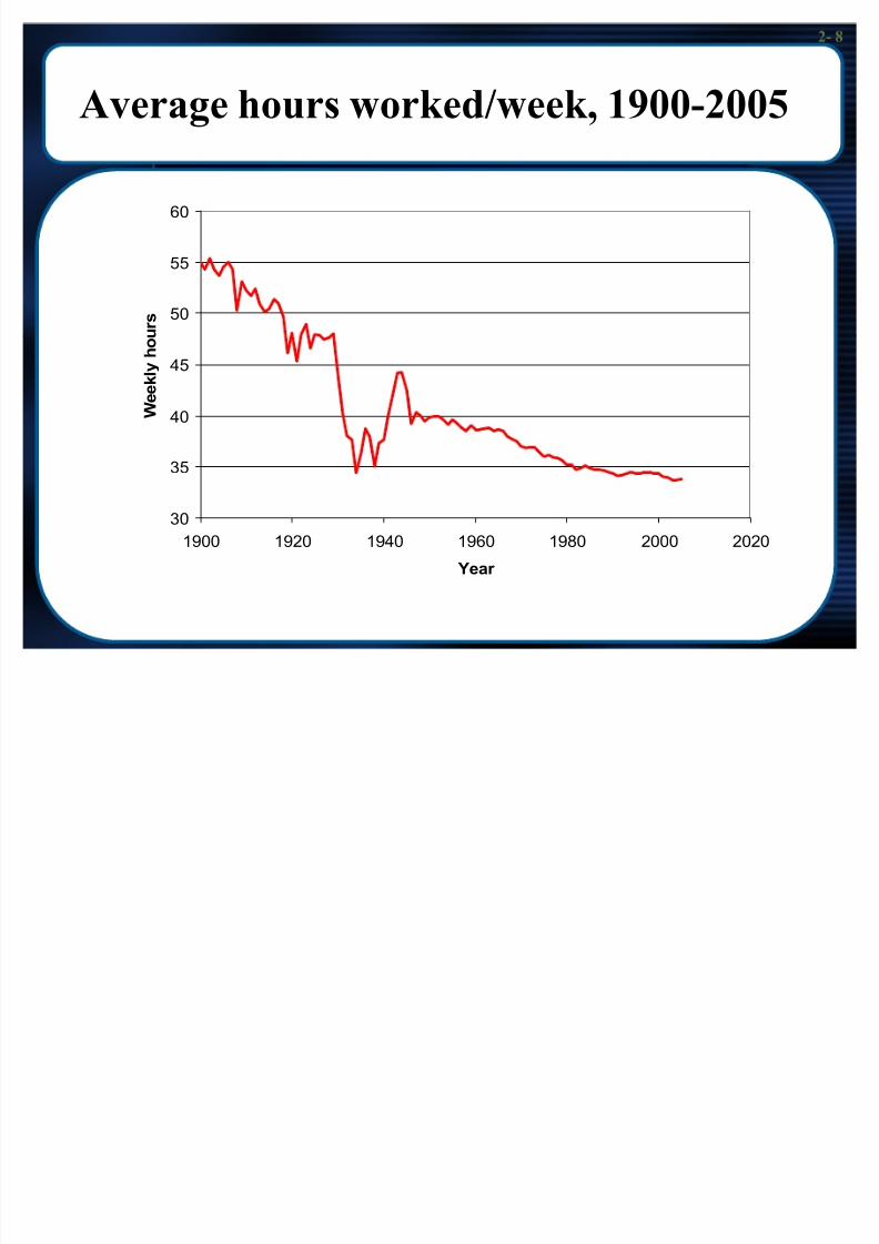
Facts about labour supply (in the USA)

8/3/2019 Chap002 Modified
http://slidepdf.com/reader/full/chap002-modified 11/76
2- 11
Facts about labour supply (in the USA)
- Mor e women than men work part-time
- Mor e men who ar e high school drop outs work than women who
ar e high school drop outs
- White men have higher partici pation rates and hour s of work than
black men

8/3/2019 Chap002 Modified
http://slidepdf.com/reader/full/chap002-modified 12/76
2- 12
Worker Performance
Neo-Classical Model of Labor -Leisur e Choice
Classical consumer problem with 2 caveats- Work is µ bad¶ (leisur e is a good)- Unear ned income deliver s a discontinuity in the budget constraint
Building bock s:- utility function- budget constraint
- time constraint
Solve for :- inter ior solution (intensive mar gin)- Partici pation (extensive mar gin)

8/3/2019 Chap002 Modified
http://slidepdf.com/reader/full/chap002-modified 13/76
2- 13
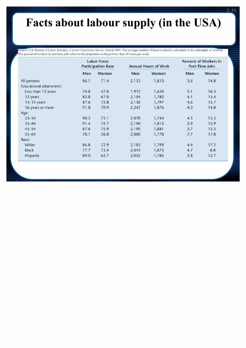
Utility function and Indifference Curves
U=f(C, L)
- C: consumption ($ value)
- L=Leisur e
Indiff er ence cur ves
- Downwar d sloping (indicates the trade off between consumption
and leisur e)
Higher cur ves = higher utility
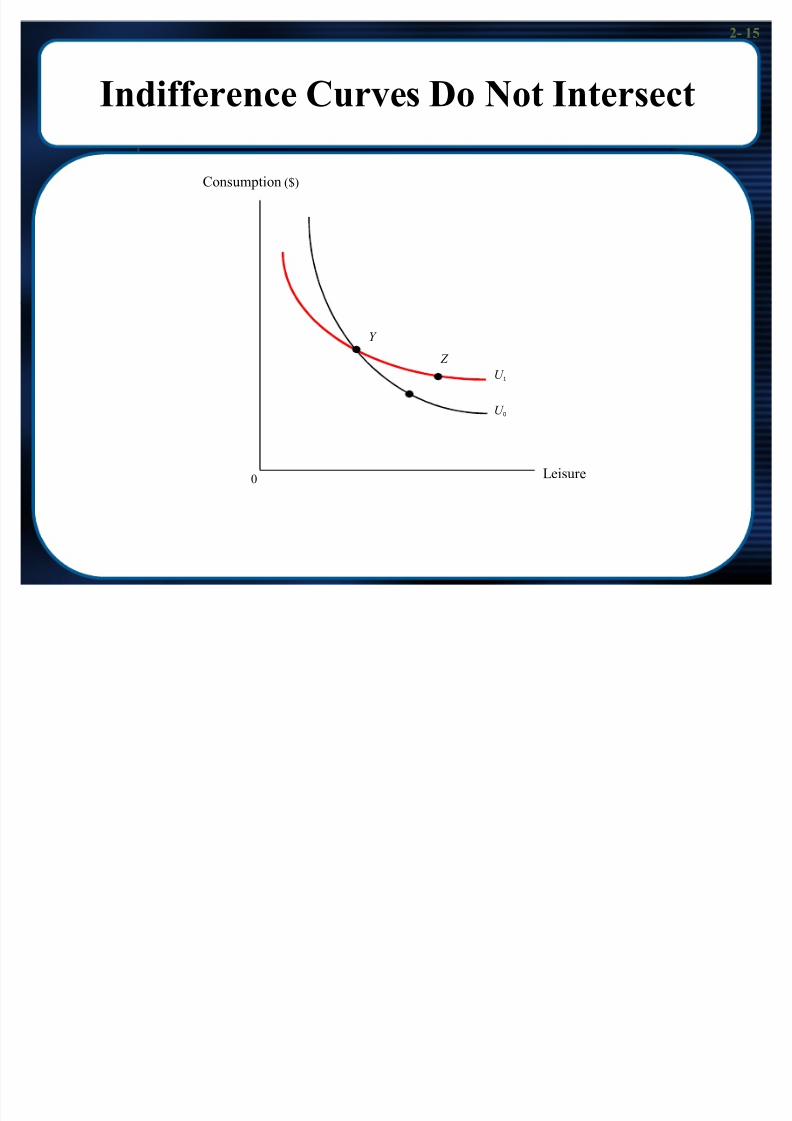
Do not inter sect
Convex to the or igin (indicating that opportunity costs incr ease)
8/3/2019 Chap002 Modified
http://slidepdf.com/reader/full/chap002-modified 14/76
2- 14
Indifference Curves
Consumption ($)
500
450
400
40,000 Utils
25,000 Utils
Hour s of
Leisur e150125100+Hour s of
work
8/3/2019 Chap002 Modified
http://slidepdf.com/reader/full/chap002-modified 15/76
2- 15
Indifference Curves Do Not Intersect
U 0
U 1
Y
Z
0 Leisur e
Consumption ($)
8/3/2019 Chap002 Modified
http://slidepdf.com/reader/full/chap002-modified 16/76
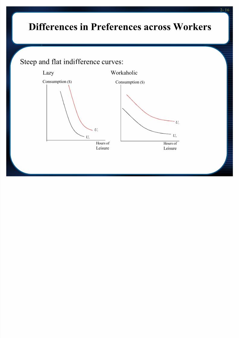
2- 16
Differences in Preferences across Workers
Stee p and flat indiff er ence cur ves:
Lazy Workaholic
U 0U 0
U 1
U 1
Consumption ($) Consumption ($)
Hour s of
Leisur eHour s of
Leisur e
8/3/2019 Chap002 Modified
http://slidepdf.com/reader/full/chap002-modified 17/76
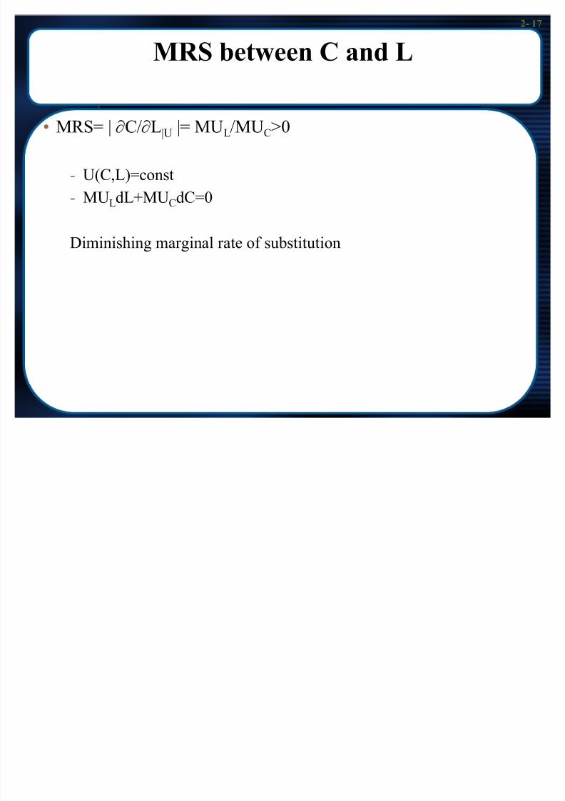
2- 17
MRS between C and L
MRS=| xC/xL|U |= MUL/MUC>0
- U(C,L)=const
- MULdL+MUCdC=0
Diminishing mar ginal rate of substitution
8/3/2019 Chap002 Modified
http://slidepdf.com/reader/full/chap002-modified 18/76
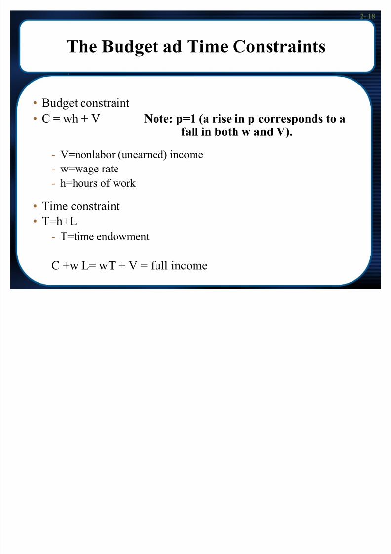
2- 18
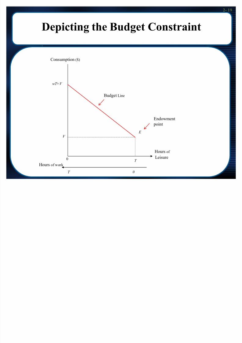
The Budget ad Time Constraints
Budget constraint
C = wh + V Note: p=1 (a rise in p corresponds to a
fall in both w and V).- V=nonlabor (unear ned) income
- w=wage rate
- h=hour s of work
Time constraint T=h+L
- T=time endowment
C +w L= wT + V = full income
8/3/2019 Chap002 Modified
http://slidepdf.com/reader/full/chap002-modified 19/76
2- 19
Depicting the Budget Constraint
T
E
V
wT+V
0
Hour s of
Leisur e
Consumption ($)
Budget Line
Endowment
point
Hour s of work
0T
8/3/2019 Chap002 Modified
http://slidepdf.com/reader/full/chap002-modified 20/76
2- 20
The Hours of Work Decision
O ptimal consumption is given by the point wher e the budget
line is tangent to the indiff er ence cur ve
MRS =w
Max U(C,L)
s.t. C +w L= wT + V
FOC: MUC= P
MUL= P w
8/3/2019 Chap002 Modified
http://slidepdf.com/reader/full/chap002-modified 21/76
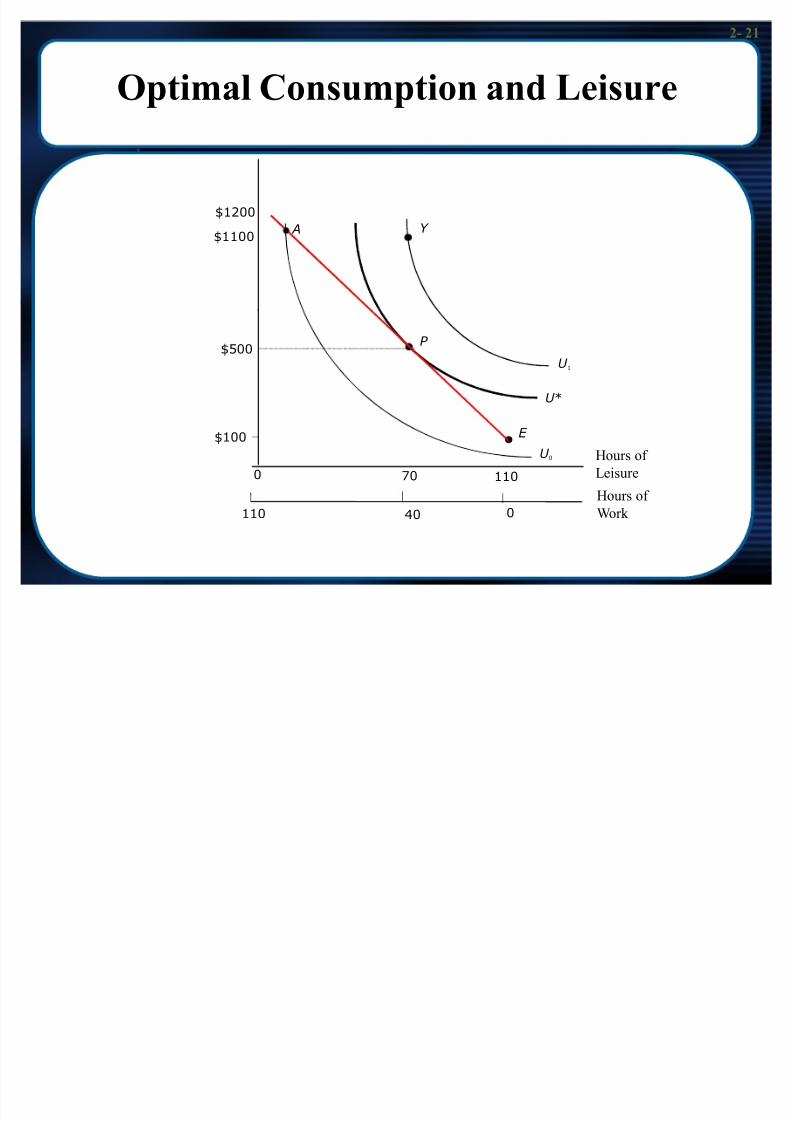
2- 21
Optimal Consumption and Leisure
$1100
$1200
A Y
$500P
U 1
$100
U 0
U *
E
110
110
40
70
0
0
Hour s of
Work
Hour s of
Leisur e
8/3/2019 Chap002 Modified
http://slidepdf.com/reader/full/chap002-modified 22/76
2- 22
Optimal Consumption and Leisure
At A: subjective evaluation of C-L tradeoff > mark et
evaluation
MRS=2W=1
Work er willing to give up 2 units of C for one extra unit of L
Able to cut his C by 1 unit for 1 extra unit of L
Not optimal: it pays to work less (consume mor e L)
w=pr ice of leisur e

8/3/2019 Chap002 Modified
http://slidepdf.com/reader/full/chap002-modified 23/76
2- 23
The Effect of a Change in Nonlabor Income on
Hours of Work
An increase in nonlabor income leads to a parallel, upward shift in the budget line, moving the
worker from point P0 to point P1. If leisure is a normal good, hours of work fall.
F 1
P 1
$200
U 1
U 0E 1
E 0
P 0
70 80 110
F 0
$100
Hour s of Leisur e
Consumption ($)
8/3/2019 Chap002 Modified
http://slidepdf.com/reader/full/chap002-modified 24/76
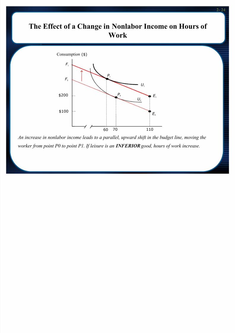
2- 24
The Effect of a Change in Nonlabor Income on Hours of
Work
An increase in nonlabor income leads to a parallel, upward shift in the budget line, moving the
worker from point P0 to point P1. If leisure is an INFERIOR good, hours of work increase.
F 1
P 1
$200
U 1
U 0
E 1
E 0
P 0
7060 110
F 0
$100
Consumption ($)

8/3/2019 Chap002 Modified
http://slidepdf.com/reader/full/chap002-modified 25/76
2- 25
The Effect of a Change in Nonlabor Income
on Hours of Work
Incr ease in nonlabor income allows work er to ³ jump´ to higher
indiff er ence cur ve, indicating the Income Effect
- Leisur e can be tr eated as a normal good or as an inf er ior good
- R easonable to assume that is a NORMAL good
8/3/2019 Chap002 Modified
http://slidepdf.com/reader/full/chap002-modified 26/76
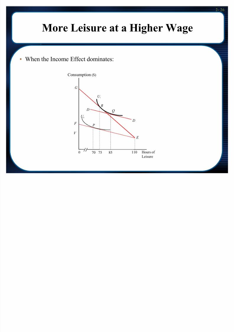
2- 26
More Leisure at a Higher Wage
When the Income Eff ect dominates:
G
U 1
Q D
D
R
P
U 0
V
F
E
8575 1100 70 Hour s of
Leisur e
Consumption ($)
8/3/2019 Chap002 Modified
http://slidepdf.com/reader/full/chap002-modified 27/76
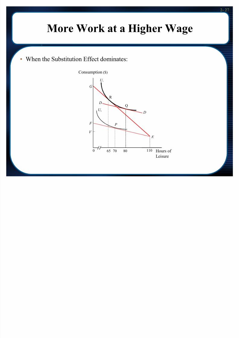
2- 27
More Work at a Higher Wage
When the Substitution Eff ect dominates:
G
D
D
F
E
U 1
Q
R
P
U 0
V
8070 1100 65 Hour s of
Leisur e
Consumption ($)

8/3/2019 Chap002 Modified
http://slidepdf.com/reader/full/chap002-modified 28/76
2- 28
Ambiguous Relationship: Hours Worked and Wage
Rates
As wages change holding real income constant, changes in
consumption-leisur e bundle indicate the Substitution Effect
If the Substitution Eff ect is gr eater than the Income Eff ect, then
hour s of work incr ease when the wage rate r ises
If the Income Eff ect is gr eater than the Substitution Eff ect, then hour s of work decr eases when the wage rate r ises.

8/3/2019 Chap002 Modified
http://slidepdf.com/reader/full/chap002-modified 29/76
2- 29
Ambiguous Relationship: Hours Worked and
Wage Rates
At optimum
h*=g(w, V+wh)
xh*/xw = xg/x w|U* + (xg/xV) h ><0 ? (1)
subst. inc.
>0 <0 IF L is NORMAL!!!!!!!!
The flatter the IC, the mor e lik ely the subst eff ect dominates

8/3/2019 Chap002 Modified
http://slidepdf.com/reader/full/chap002-modified 30/76
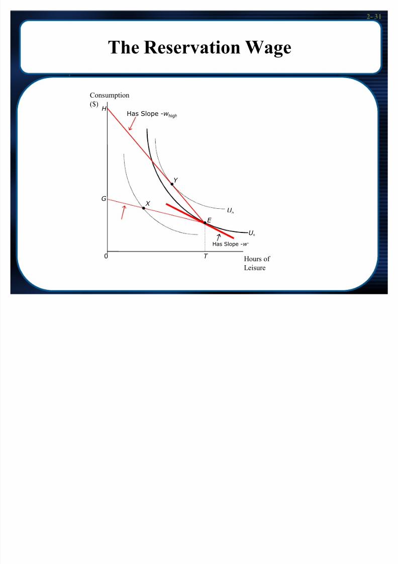
2- 30
To Work or Not to Work?
Ar e the ³terms of trade´ suff iciently attractive to br i be a work er to enter the labor mark et?
R eser vation wage: the minimum level of wages that would mak e the per son indiff er ent between work ing and not work ing
- Rule 1: if the mark et wage is less than the r eser vation wage, then the per son will not work
- Rule 2: the r eser vation wage incr eases as nonlabor income incr eases
8/3/2019 Chap002 Modified
http://slidepdf.com/reader/full/chap002-modified 31/76
2- 31
The Reservation Wage
H
Y
G X
U H
E
U 0
Hour s of
Leisur e
T 0
Has Slope -w high
Has Slope -w b
Consumption
($)

8/3/2019 Chap002 Modified
http://slidepdf.com/reader/full/chap002-modified 32/76
2- 32
For standar d budget lines
w*=MRS |L=T
Cor ner solution (work er would lik e to buy mor e leisur e than C)
If V incr eases , w* r ises
Stee per IC associated to higher w*
(w* inde pendent of w)
For individuals out of work a r ise in w only induces a
substitution eff ect
The Reservation Wage

8/3/2019 Chap002 Modified
http://slidepdf.com/reader/full/chap002-modified 33/76
2- 33
Labor Supply Curve
h*=T-L*=h(w,V)
Hour s of
Work
0
Wage Rate ($)
4020 30
10
20
25

8/3/2019 Chap002 Modified
http://slidepdf.com/reader/full/chap002-modified 34/76
2- 34
Labor Supply Curve
R elationshi p between hour s work ed and the wage rate
- For w slightly above w*, the labor supply cur ve is
positively sloped (substitution eff ect dominates)
- If the income eff ect begins to dominate, hour s of work decline as wage rates incr ease (a negatively sloped labor supply cur ve)

8/3/2019 Chap002 Modified
http://slidepdf.com/reader/full/chap002-modified 35/76
2- 35
Labor Supply Elasticity
Elasticity of (individual LS) = % change in hours work ed/% change in wage rate =
W=[xh/xw] w/h = [xh/h] w/ xw = x lnh / xlnw
Labor supply elasticity <1 means ³inelastic´
If elasticity of LS negative income eff ect dominates and ear nings grow less than proportionally as wages incr ease
x ln wh / xln w = W +1
8/3/2019 Chap002 Modified
http://slidepdf.com/reader/full/chap002-modified 36/76
2- 36
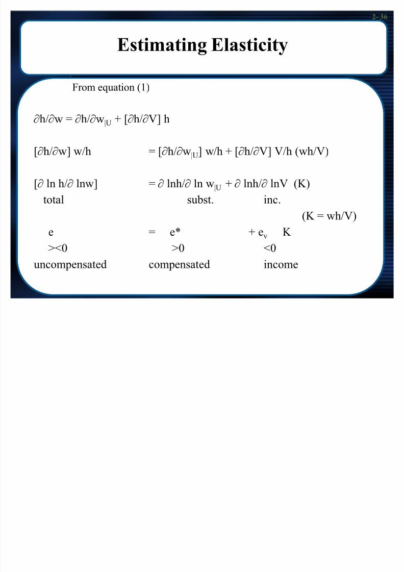
Estimating Elasticity
From equation (1)
xh/xw = xh/xw|U + [xh/xV] h
[xh/xw] w/h = [xh/xw|U] w/h + [xh/xV] V/h (wh/V)
[x ln h/x lnw] = x lnh/x ln w|U + x lnh/x lnV (K)
total subst. inc.
(K = wh/V)e = e* + ev K
><0 >0 <0
uncompensated compensated income
8/3/2019 Chap002 Modified
http://slidepdf.com/reader/full/chap002-modified 37/76
2- 37
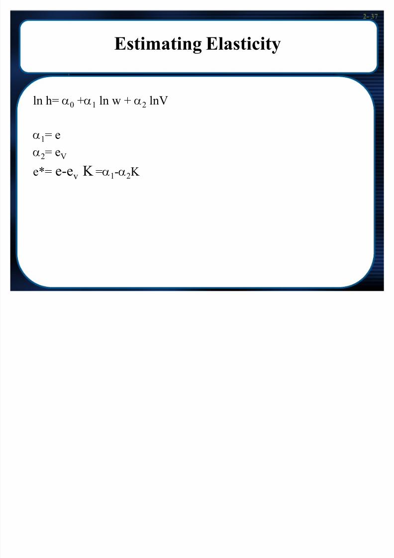
Estimating Elasticity
ln h= E0 +E1 ln w + E2 lnV
E1= e E2= eV
e*= e-ev K =E1-E2K
8/3/2019 Chap002 Modified
http://slidepdf.com/reader/full/chap002-modified 38/76
2- 38
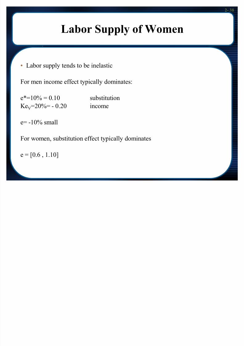
Labor Supply of Women
Labor supply tends to be inelastic
For men income eff ect typically dominates:
e*=10% = 0.10 substitution
K eV=20%= - 0.20 income
e= -10% small
For women, substitution eff ect typically dominates
e = [0.6 , 1.10]

8/3/2019 Chap002 Modified
http://slidepdf.com/reader/full/chap002-modified 39/76
2- 39
Derivation of the Market Labor Supply Curve from
the Supply Curves of Individual Workers
0 0 0
w ~ B
w ~ A
w ~ B
w ~ A
h A
h A +
h B
( a) Alice ( b) Br enda ( c) Mark et
Wage Rate ($) Wage Rate ($) Wage Rate ($)
Hour s of Work
h A
h B
Note: when we discuss elasticity of aggr egate labor supply we
generally r ef er to % change in PARTICIPATION for a 1% change in
wages
2 40
8/3/2019 Chap002 Modified
http://slidepdf.com/reader/full/chap002-modified 40/76
2- 40
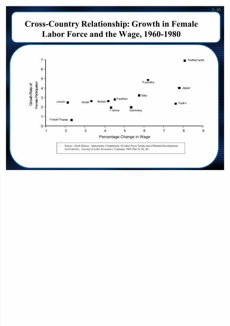
Cross-Country Relationship: Growth in Female
Labor Force and the Wage, 1960-1980
Sour ce: Jacob Mincer , ³Inter country Compar isons of Labor For ce Tr ends and of R elated Developments:
An Over view,´ J ournal of Labor E conomics 3 (January 1985, Part 2): S2, S6.
1 2 3 4 5 6 7 8 9
Percentage Change in Wage
0
1
2
3
4
5
6
7
F e m a l e P a r t i c i p a t i o n
G r o w t h R a t e o f
n te tates
Israel Britain
rance
we en
Germany
Italy
ustra a
pa n
Japan
et er an s
2 41

8/3/2019 Chap002 Modified
http://slidepdf.com/reader/full/chap002-modified 41/76
2- 41
Policy Application: Welfare Programs and Work
Incentives
Cash grants r educe wage incentives
Welfar e programs cr eate work disincentives
Welfar e r educes supply of labor by granting nonlabor income,
which raises r eser vation wage
2 42
8/3/2019 Chap002 Modified
http://slidepdf.com/reader/full/chap002-modified 42/76
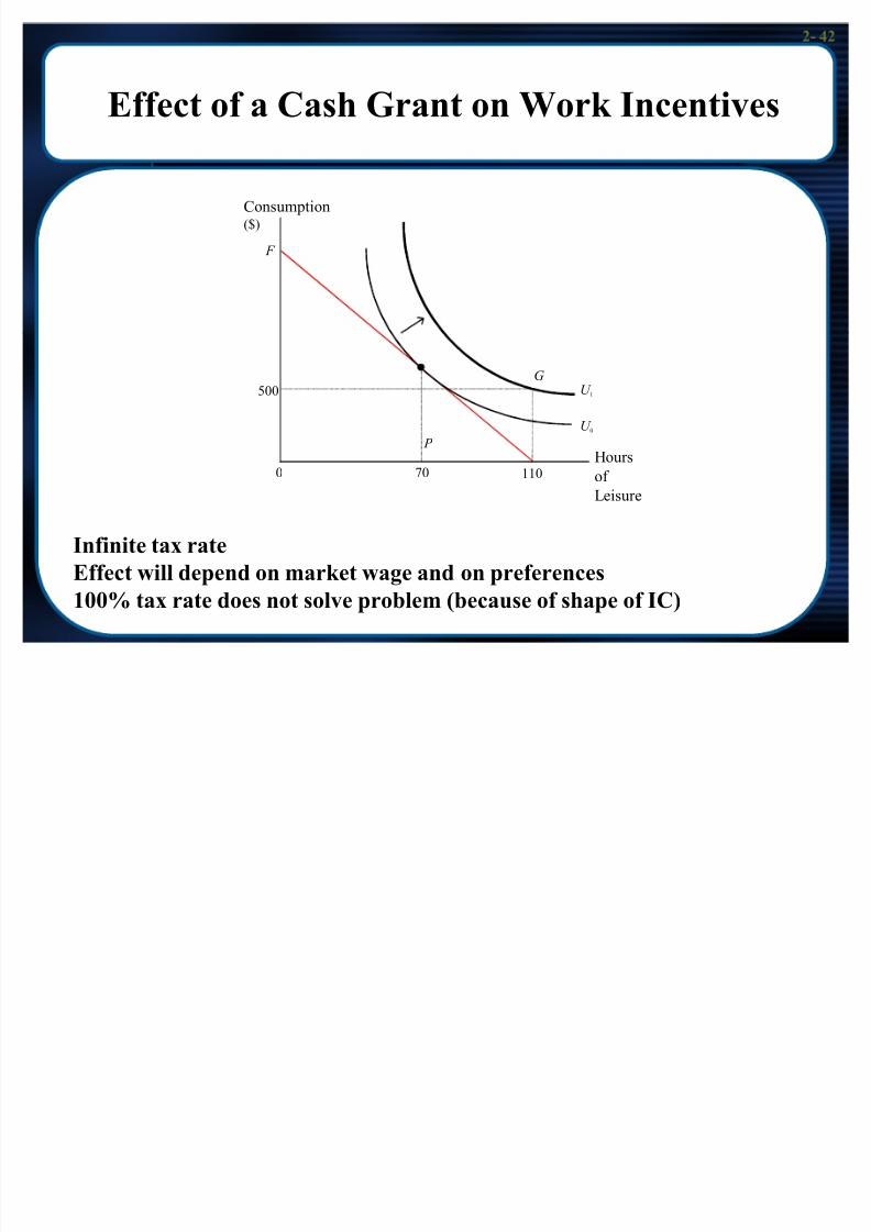
2- 42
Effect of a Cash Grant on Work Incentives
F
Consumption($)
500
Hour s of
Leisur e
0 11070
G
U 1
U 0 P
Infinite tax rate
Effect will depend on market wage and on preferences
100% tax rate does not solve problem (because of shape of IC)
2 43

8/3/2019 Chap002 Modified
http://slidepdf.com/reader/full/chap002-modified 43/76
2- 43
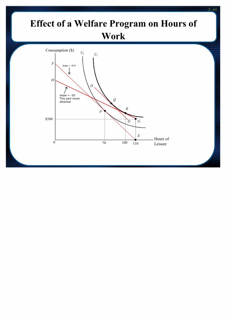
$500 cash grant
taxed at 50% for every $ ear ned (up to when exhausted)
Effect of a Welfare Program on Hours of
Work
2 44
8/3/2019 Chap002 Modified
http://slidepdf.com/reader/full/chap002-modified 44/76
2- 44
Effect of a Welfare Program on Hours of
Work
Hour s of
Leisur e
$500
U 0 U 1
G
E
P
F
R
Q
H
D
D
0 11010070
slope = -$5This part never
attained
slope = -$10
Consumption ($)
2 45

8/3/2019 Chap002 Modified
http://slidepdf.com/reader/full/chap002-modified 45/76
2- 45
Effect of a Welfare Program on Hours of
Work
Income and substitution eff ects act in same dir ection
In pr inci ple work er s to the left of inter section btw 2 budget lines
can work less
2 46

8/3/2019 Chap002 Modified
http://slidepdf.com/reader/full/chap002-modified 46/76
2- 46
Policy Application: The Earned-Income Tax
Credit
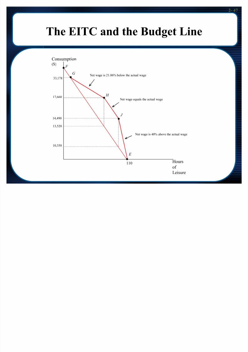
Cr edit of 40 % on labor ear nings as long she ear ns < $10,350. w(1.4)
Cr edit capped at $4,140 = (0.40 * 10,350)
At that point work er mak es 14,490
This maximum amount can be r etained as long as work er ear ns no mor e that $13,520
At that point work er mak es 17,760
Tax cr edit phased out at rate 21.06% Cr edit is exhausted when work er mak es $33,178
[17,660-13,520*(1-.2106)]/.2106
2- 47
8/3/2019 Chap002 Modified
http://slidepdf.com/reader/full/chap002-modified 47/76
2- 47
The EITC and the Budget Line
Hour s
of
Leisur e
Consumption($)
110
10,350
13,520
14,490
17,660
33,178
E
J
H
G
F
Net wage is 40% above the actual wage
Net wage equals the actual wage
Net wage is 21.06% below the actual wage
2- 48

8/3/2019 Chap002 Modified
http://slidepdf.com/reader/full/chap002-modified 48/76
2- 48
Policy Application: The Earned-Income Tax
Credit
2- 49

8/3/2019 Chap002 Modified
http://slidepdf.com/reader/full/chap002-modified 49/76
2 49
The Impact of the EITC on Labor Supply
EITC incr eases LFP of non-work er s produces an income eff ect - hour s work ed should
change (even among non tar get group)
2- 50

8/3/2019 Chap002 Modified
http://slidepdf.com/reader/full/chap002-modified 50/76
2 50
Taxation and labor supply
The wage rate that is r elevant for labor supply decisions
is the tak e home wage.
Labor supply function de pends on the net wage.
Proportional taxation: flatter budget line
Progr essive tax: k ink ed budget line
O ptimum can be at k ink for many work er s (cor ner
solution)
2- 51
8/3/2019 Chap002 Modified
http://slidepdf.com/reader/full/chap002-modified 51/76
2 51
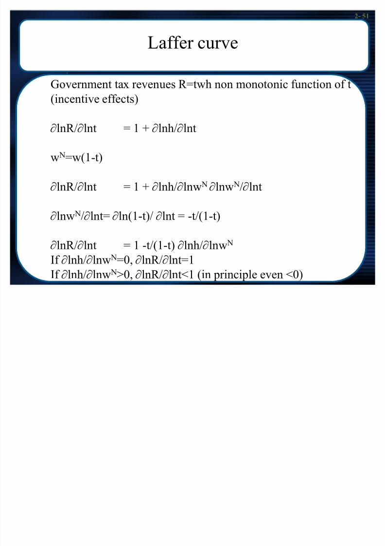
Laff er cur ve
Gover nment tax r evenues R=twh non monotonic function of t
(incentive eff ects)
xlnR/xlnt = 1 + xlnh/xlnt
w N=w(1-t)
xlnR/xlnt = 1 + xlnh/xlnw N xlnw N/xlnt
xlnw N/xlnt= xln(1-t)/ xlnt = -t/(1-t)
xlnR/xlnt = 1 -t/(1-t) xlnh/xlnw N
If xlnh/xlnw N=0, xlnR/xlnt=1
If xlnh/xlnw N>0, xlnR/xlnt<1 (in pr inci ple even <0)
2- 52

8/3/2019 Chap002 Modified
http://slidepdf.com/reader/full/chap002-modified 52/76
2 52
Extensions
³Static´ model is not a complete de piction of how we allocate
our time
We extend the basic model to consider:- The long run
- Hus band-wif e joint-decisions to supply labor
2- 53
8/3/2019 Chap002 Modified
http://slidepdf.com/reader/full/chap002-modified 53/76
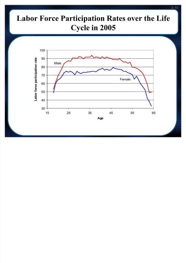
Labor Force Participation Rates over the Life
Cycle in 2005
30
40
50
60
70
80
90
100
15 25 35 45 55 65
Age
L a
b o r f o r c e p a r t i c i p a t i o n r a t e
Male
Female
2- 54
8/3/2019 Chap002 Modified
http://slidepdf.com/reader/full/chap002-modified 54/76
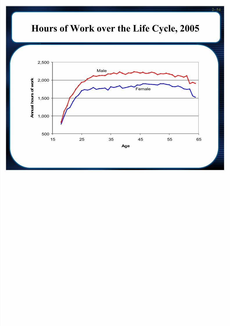
Hours of Work over the Life Cycle, 2005
500
1,000
1,500
2,000
2,500
15 25 35 45 55 65
Age
A n n u a l h o u r s o f w o
r k
Male
Female
2- 55

8/3/2019 Chap002 Modified
http://slidepdf.com/reader/full/chap002-modified 55/76
Labor supply over the life cycle
Wage rates change over the work er ¶s lif e cycle
- Wages ar e low when young
- Wages r ise with time and peak around age 50- Wages decline or r emain stable after the age of 50
Change in wage over the lif e cycle is an ³evolutionary´ wage
change alter ing the pr ice of leisur e
2- 56

8/3/2019 Chap002 Modified
http://slidepdf.com/reader/full/chap002-modified 56/76
The Life Cycle Path of Wages and Hours for a
Typical Worker
Age
Wage
Rate
50 Age
Hour s of
work
50
2- 57
8/3/2019 Chap002 Modified
http://slidepdf.com/reader/full/chap002-modified 57/76
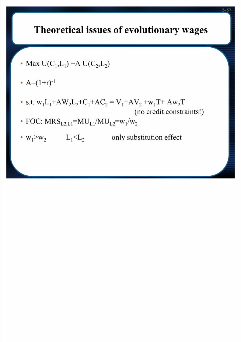
Theoretical issues of evolutionary wages
Max U(C1,L1) +A U(C2,L2)
A=(1+r)-1
s.t. w1L1+AW2L2+C1+AC2 = V1+AV2 +w1T+ Aw2T
(no cr edit constraints!)
FOC: MRSL2,L1=MUL1/MUL2=w1/w2
w1>w2 L1<L2 only substitution eff ect
2- 58

8/3/2019 Chap002 Modified
http://slidepdf.com/reader/full/chap002-modified 58/76
Theoretical issues of evolutionary wages
Positive r elationshi p between changes in hour s or work and changes in the wage rate
The prof ile of hour s of work over the lif e cycle will have the same shape as the age-ear nings prof ile
Intertemporal substitution hypothesis: people substitute their time over the lif e cycle to tak e advantage of changes in the
pr ice of leisur e
2- 59

8/3/2019 Chap002 Modified
http://slidepdf.com/reader/full/chap002-modified 59/76
Hours of Work over the Life Cycle for Two
Workers with Different Wage Paths
Age
Jack
t * Age t *
Joe
Wage Rate Hour s of Work
Jack
Joe (if substitution eff ect
dominates)
Joe (if income eff ect
dominates)
Joe¶s wage exceeds Jack ¶s at every age. Although both Joe and Jack work mor e
hour s when the wage is high, Joe work s mor e hour s than Jack only if the
substitution eff ect dominates. If the income eff ect dominates, Joe work s f ewer
hour s than Jack .
2- 60
8/3/2019 Chap002 Modified
http://slidepdf.com/reader/full/chap002-modified 60/76
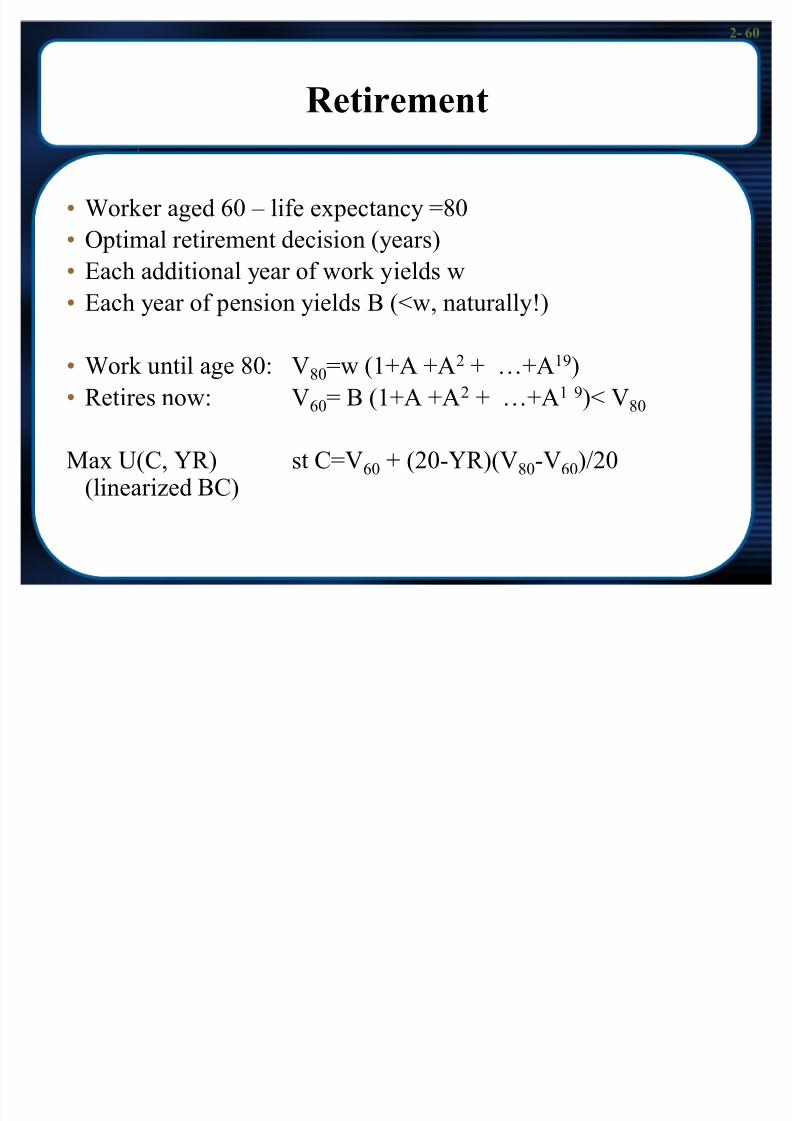
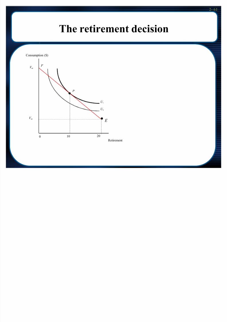
Retirement
Work er aged 60 ± lif e ex pectancy =80
O ptimal r etir ement decision (year s)
Each additional year of work yields w
Each year of pension yields B (<w, naturally!)
Work until age 80: V80=w (1+A +A2 + «+A19)
R etir es now: V60= B (1+A +A2 + «+A1 9)< V80
Max U(C, YR) st C=V60 + (20-YR)(V80-V60)/20(linear ized BC)
2- 61
8/3/2019 Chap002 Modified
http://slidepdf.com/reader/full/chap002-modified 61/76
The retirement decision
Consumption ($)
20
P
U 0
U 1
V 60
V 80
R etir ement
F
100
E
2- 62
8/3/2019 Chap002 Modified
http://slidepdf.com/reader/full/chap002-modified 62/76
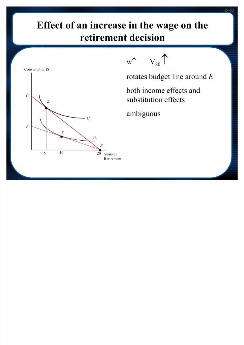
Effect of an increase in the wage on the
retirement decision
wo V80o
rotates budget line around E
both income eff ects and substitution eff ects
ambiguous
R
P
20105
U 1
U 0
G
F
E
Consumption ($)
Year s of
R etir ement
2- 63
8/3/2019 Chap002 Modified
http://slidepdf.com/reader/full/chap002-modified 63/76
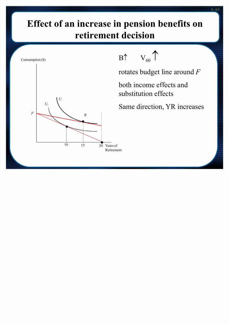
Effect of an increase in pension benefits on
retirement decision
2010 15
R
U 1
U 0
F
Consumption ($)
Year s of
R etir ement
Bo V60o
rotates budget line around F
both income eff ects and substitution eff ects
Same dir ection, YR incr eases
2- 64

8/3/2019 Chap002 Modified
http://slidepdf.com/reader/full/chap002-modified 64/76
Policy Application: the decline in work
attachment among older workers
Older work er s have lower partici pation rates
Work disincentives/ Disability benef its
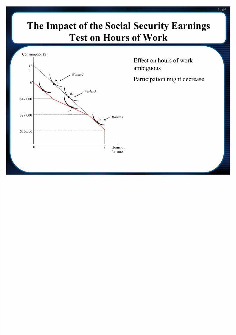
Social Secur ity Ear nings Test
Assume r etir ement benef it = 10K
r etir ees can ear n <=$17K without losing r etir ement benef its
If ear nings>$17K every $3 of income r educes benef its by $1 R etir ee exhaust r etir ement benef it when he ear ns 47K
2- 65
8/3/2019 Chap002 Modified
http://slidepdf.com/reader/full/chap002-modified 65/76
The Impact of the Social Security Earnings
Test on Hours of Work
$47,000
$10,000
$27,000
Consumption ($)
H
H R2
P1
R3
P 3
T 0 Hour s of
Leisur e
W orker 2
W orker 1
W orker 3
Eff ect on hour s of work
ambiguous
Partici pation might decr ease
2- 66

8/3/2019 Chap002 Modified
http://slidepdf.com/reader/full/chap002-modified 66/76
Allocation of Weekly Hours to Various Activities,
By Gender and Marital Status
40.2
32.9
16.7
22.2
14.3
12
34.9
23.5
77.6
76.9
78.7
79.4
22.4
24.2
22
23.8
13.5
22
15.7
19.1
0 24 48 72 96 120 144 168
Married Men
Unmarried Men
Married Women
Unmarried Women
Mark et
Work Household
Work
Per sonal Car e Passive
Leisur e
Other
2- 67

8/3/2019 Chap002 Modified
http://slidepdf.com/reader/full/chap002-modified 67/76
Household Production
Leisur e includes many forms of nonmark et work , including
household production
Why do some household member s s pecialize in the mark etsector and other member s s pecialize in the household sector?
Why marr ied women have an incentive to s pecialize in
household production?
2- 68

8/3/2019 Chap002 Modified
http://slidepdf.com/reader/full/chap002-modified 68/76
Household Production Function
Household problem Assume no leisur e!
Max U(C,Z)
s.t. C=C1+C2=w1h1+w2h2 mark et produced goods
Z=Z1+Z2=a1(T1-h1)+a2(T2-h2) home produced goods
- a1, a2= mar ginal productivity in home production
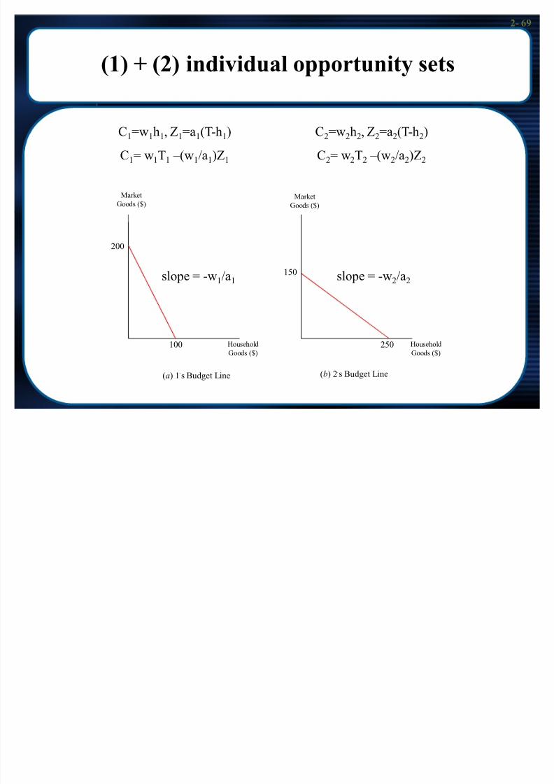
Assume w1/a1>w2/a2
Individual 1 r elatively mor e productive in mark et
(comparative advantage)
2- 69
8/3/2019 Chap002 Modified
http://slidepdf.com/reader/full/chap002-modified 69/76
(1) + (2) individual opportunity sets
200
100 Household
Goods ($)
Mark et
Goods ($)
(a) 1¶s Budget Line
slope = -w1/a1150
250 Household
Goods ($)
Mark et
Goods ($)
(b) 2¶s Budget Line
slope = -w2/a2
C1=w1h1, Z1=a1(T-h1)
C1= w1T1 ±(w1/a1)Z1
C2=w2h2, Z2=a2(T-h2)
C2= w2T2 ±(w2/a2)Z2
2- 70
8/3/2019 Chap002 Modified
http://slidepdf.com/reader/full/chap002-modified 70/76
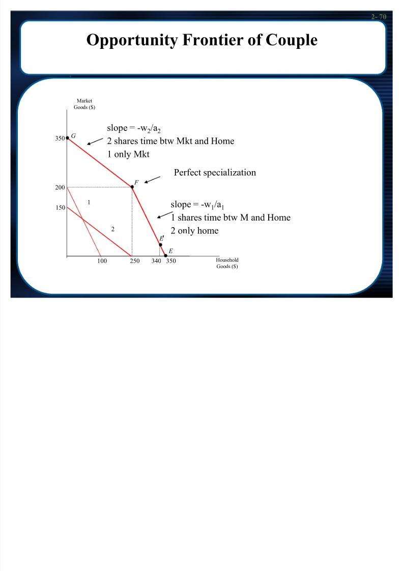
Opportunity Frontier of Couple
G350
F 200
1
2
E ¡
E
250100 350340 Household
Goods ($)
150 slope = -w1/a1
1 shar es time btw M and Home2 only home
slope = -w2/a2
2 shar es time btw Mkt and Home
1 only Mkt
Perf ect s pecialization
Mark et
Goods ($)
2- 71
8/3/2019 Chap002 Modified
http://slidepdf.com/reader/full/chap002-modified 71/76
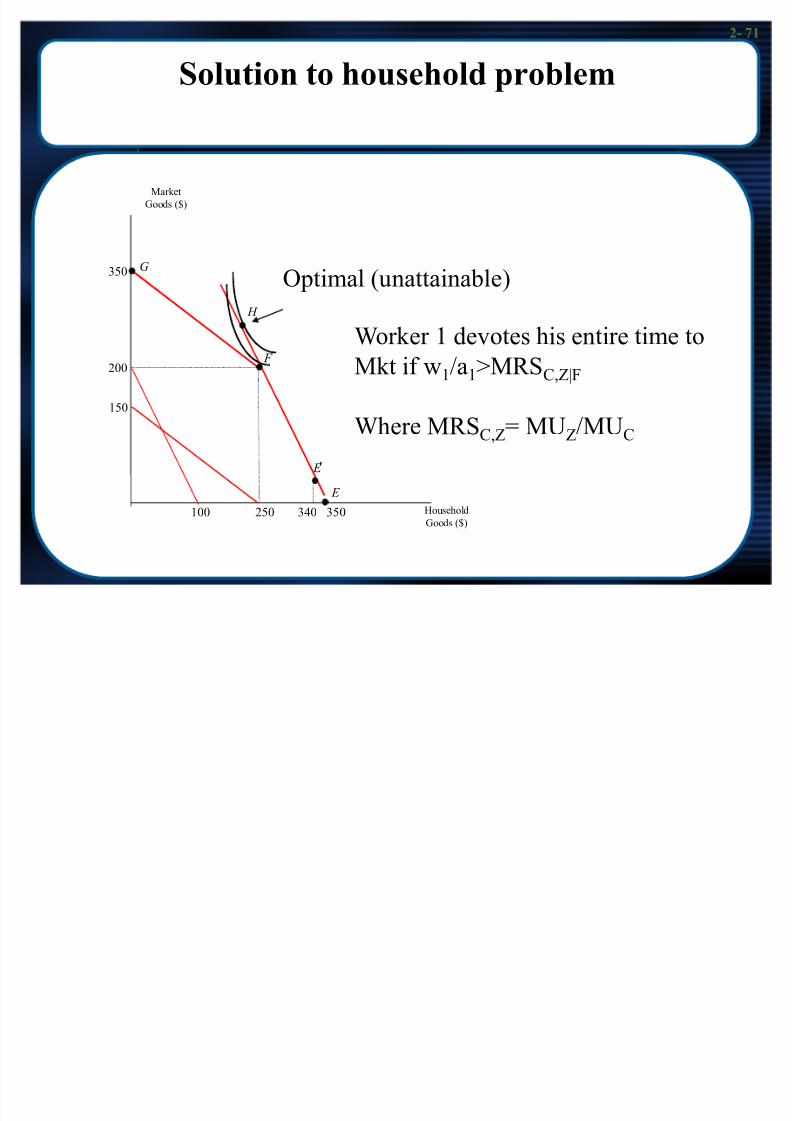
Solution to household problem
G350
F 200
E ¢
E
250100 350340 Household
Goods ($)
150
O ptimal (unattainable)
H
Work er 1 devotes his entir e time to
Mkt if w1/a1>MRSC,Z|F
Wher e MRSC,Z= MUZ/MUC
Mark etGoods ($)
2- 72
8/3/2019 Chap002 Modified
http://slidepdf.com/reader/full/chap002-modified 72/76
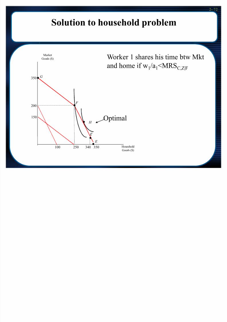
Solution to household problem
G350
F 200
E £
E
250100 350340 Household
Goods ($)
150 O ptimal H
Work er 1 shar es his time btw Mkt
and home if w1/a1<MRSC,Z|F
Mark etGoods ($)
2- 73
8/3/2019 Chap002 Modified
http://slidepdf.com/reader/full/chap002-modified 73/76
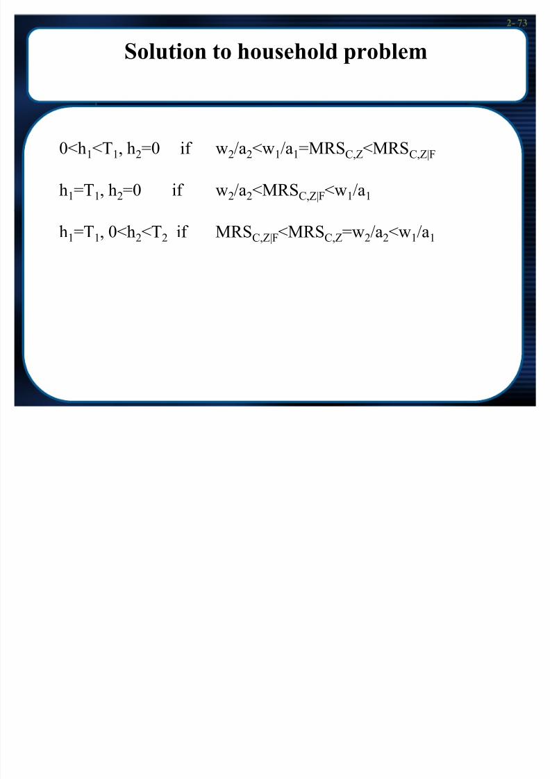
Solution to household problem
0<h1<T1, h2=0 if w2/a2<w1/a1=MRSC,Z<MRS
C,Z|F
h1=T
1, h
2=0 if w
2/a
2<MRS
C,Z|F
<w1/a
1
h1=T1, 0<h2<T2 if MRSC,Z|F<MRS
C,Z=w2/a2<w1/a1
2- 74
8/3/2019 Chap002 Modified
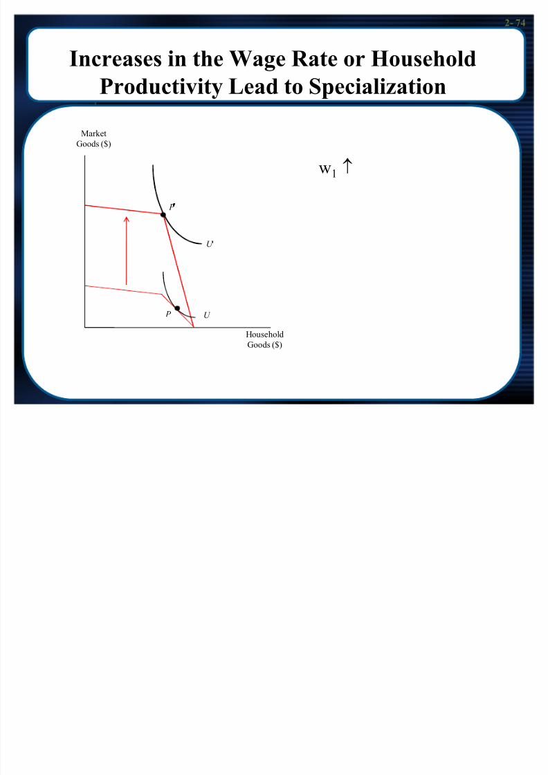
http://slidepdf.com/reader/full/chap002-modified 74/76
Increases in the Wage Rate or Household
Productivity Lead to Specialization
Household
Goods ($)
Mark et
Goods ($)
P ¤
U d
U P
w1 o
2- 75

8/3/2019 Chap002 Modified
http://slidepdf.com/reader/full/chap002-modified 75/76
Increases in the Wage Rate or Household
Productivity Lead to Specialization
Household
Goods ($)
Mark et
Goods ($)
U d
P d P
U
a2 o
2- 76

8/3/2019 Chap002 Modified
http://slidepdf.com/reader/full/chap002-modified 76/76
End of Chapter 2 (&9)