M.E. Mech. Engg.

(Design Engineering) - 2013 Course

Semester - I

Material Science and Mechanical Behavior of Materials [502202]

6. Elasto – Visco - Plasticity Visco-elasticity, rheological models, Maxwell model, Voigt model, Voigt–Maxwell model, damping, natural decay, dependence of damping and elastic modulus on frequency, thermo-elastic effect, low temperature and high temperature visco-plastic deformation models, rubber elasticity, damping, yielding, effect of strain rate, crazing.

Introduction

In classic elasticity there is no time delay between the application of a force and the deformation that it causes.

For many materials, however, there is additional time-dependent deformation that is recoverable. This is called viscoelastic or anelastic deformation.

When a load is applied to a material, there is an instantaneous elastic response, but the deformation also increases with time.

This viscoelasticity should not be confused with creep, which is time-dependent plastic deformation.

Anelastic strains in metals and ceramics are usually so small that they are ignored. In many polymers, however, viscoelastic strains can be very significant.

Anelasticity is responsible for the damping of vibrations.

A high damping capacity is desirable where vibrations might interfere with the precision of instruments or machinery and for controlling unwanted noise.

A low damping capacity is desirable in materials used for frequency standards, in bells, and in many musical instruments. Viscoelastic strains are often undesirable.

They cause sagging of wooden beams, denting of vinyl flooring by heavy furniture, and loss of dimensional stability in gauging equipment.

The energy associated with damping is released as heat, which often causes an unwanted temperature increase. Study of damping peaks and how they are affected by processing has been useful in identifying mechanisms.

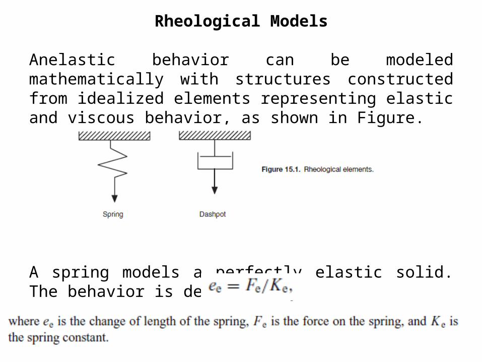
Rheological Models

Anelastic behavior can be modeled mathematically with structures constructed from idealized elements representing elastic and viscous behavior, as shown in Figure.

A spring models a perfectly elastic solid. The behavior is described by

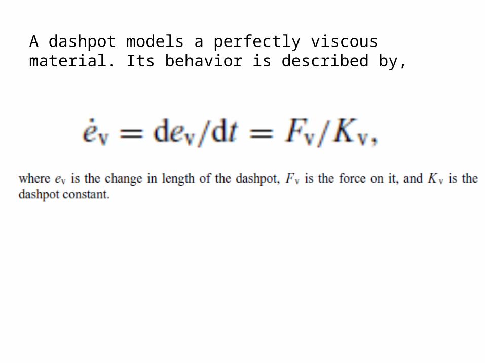
A dashpot models a perfectly viscous material. Its behavior is described by,

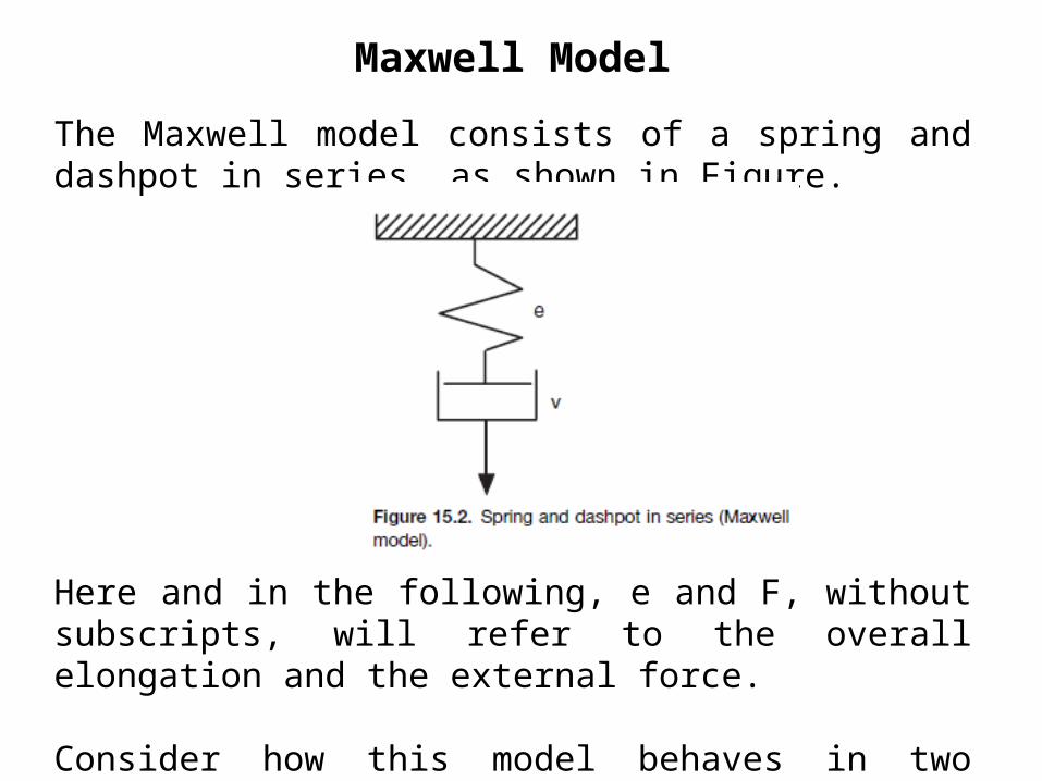
Maxwell Model

The Maxwell model consists of a spring and dashpot in series, as shown in Figure.

Here and in the following, e and F, without subscripts, will refer to the overall elongation and the external force.

Consider how this model behaves in two simple experiments.

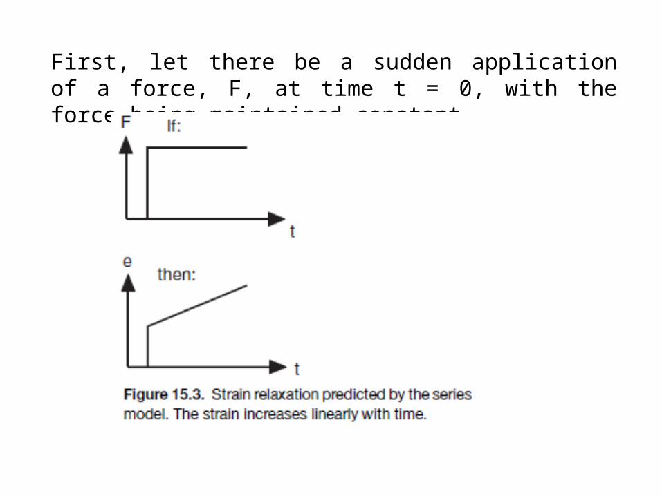
First, let there be a sudden application of a force, F, at time t = 0, with the force being maintained constant.

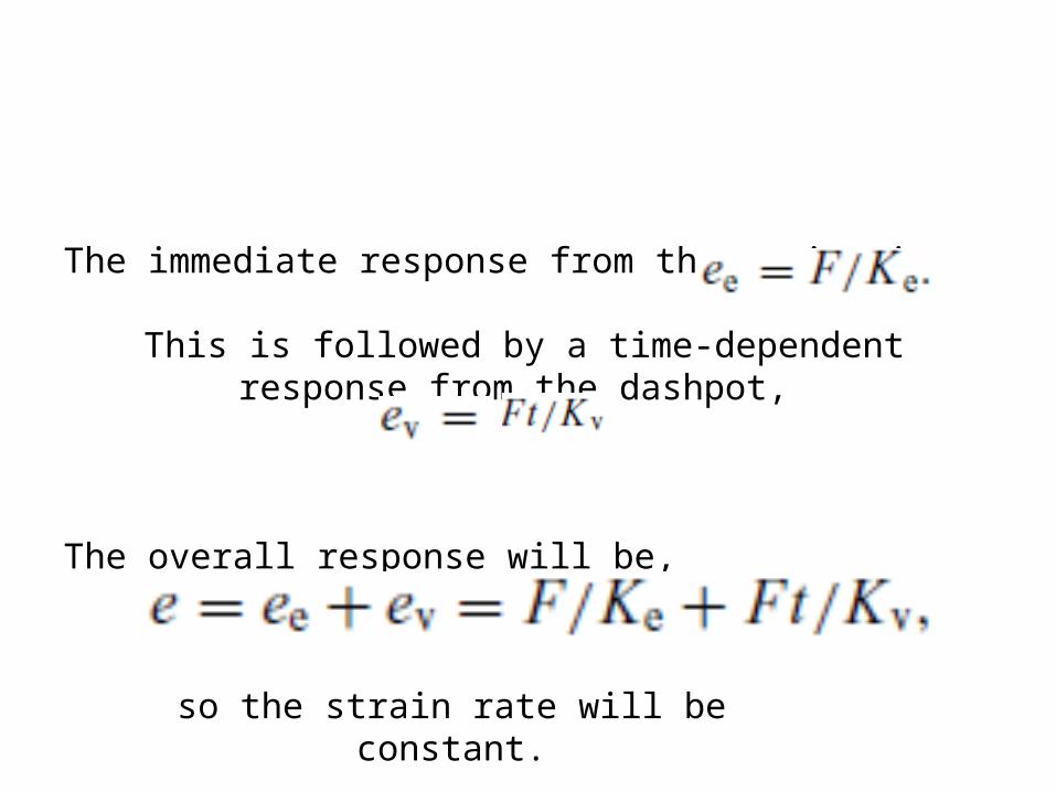
The immediate response from the spring is

This is followed by a time-dependent response from the dashpot,

The overall response will be,

so the strain rate will be constant.

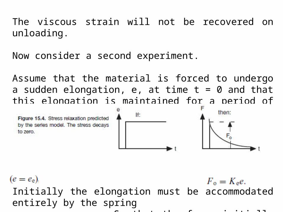
The viscous strain will not be recovered on unloading.

Now consider a second experiment.

Assume that the material is forced to undergo a sudden elongation, e, at time t = 0 and that this elongation is maintained for a period of time, as sketched in following figure,

Initially the elongation must be accommodated entirely by the spring . So that the force initially jumps to a level

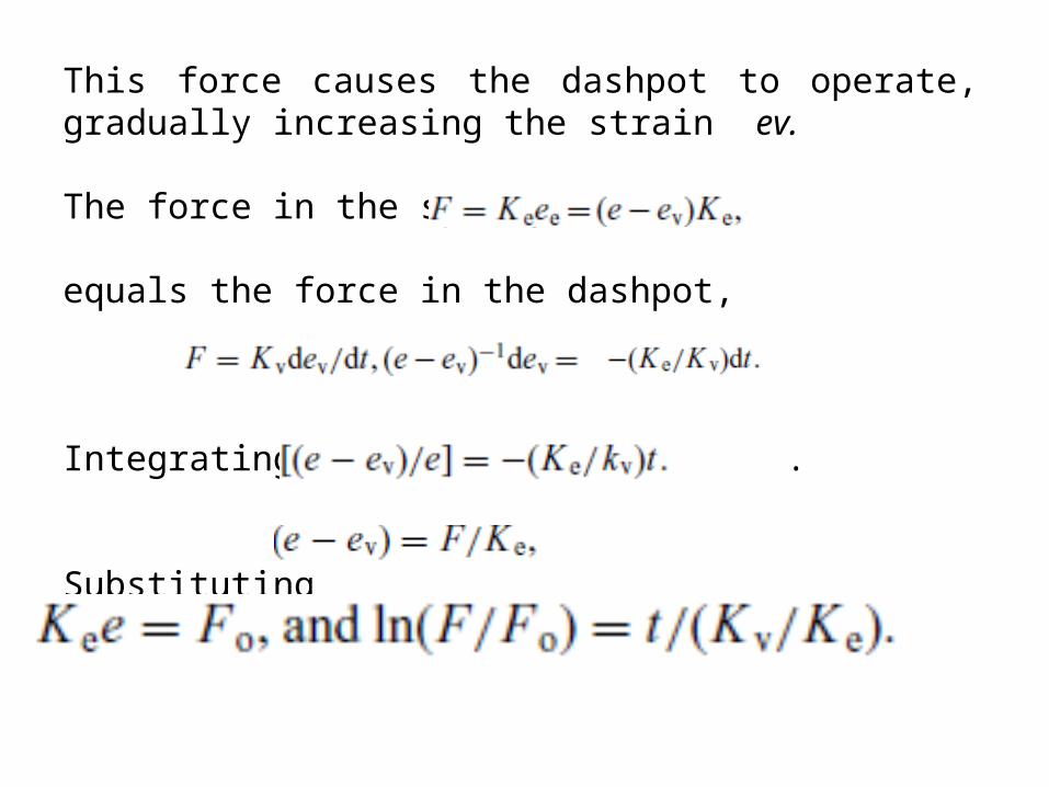
This force causes the dashpot to operate, gradually increasing the strain ev.

The force in the spring,

equals the force in the dashpot,

Integrating, ln .

Substituting

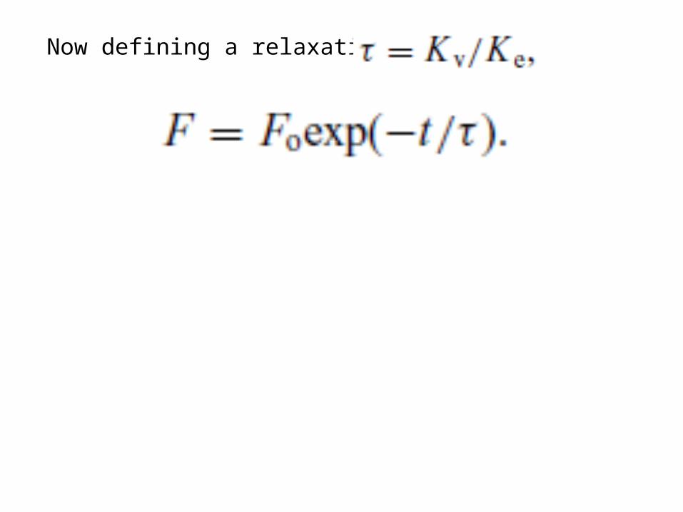
Now defining a relaxation time,

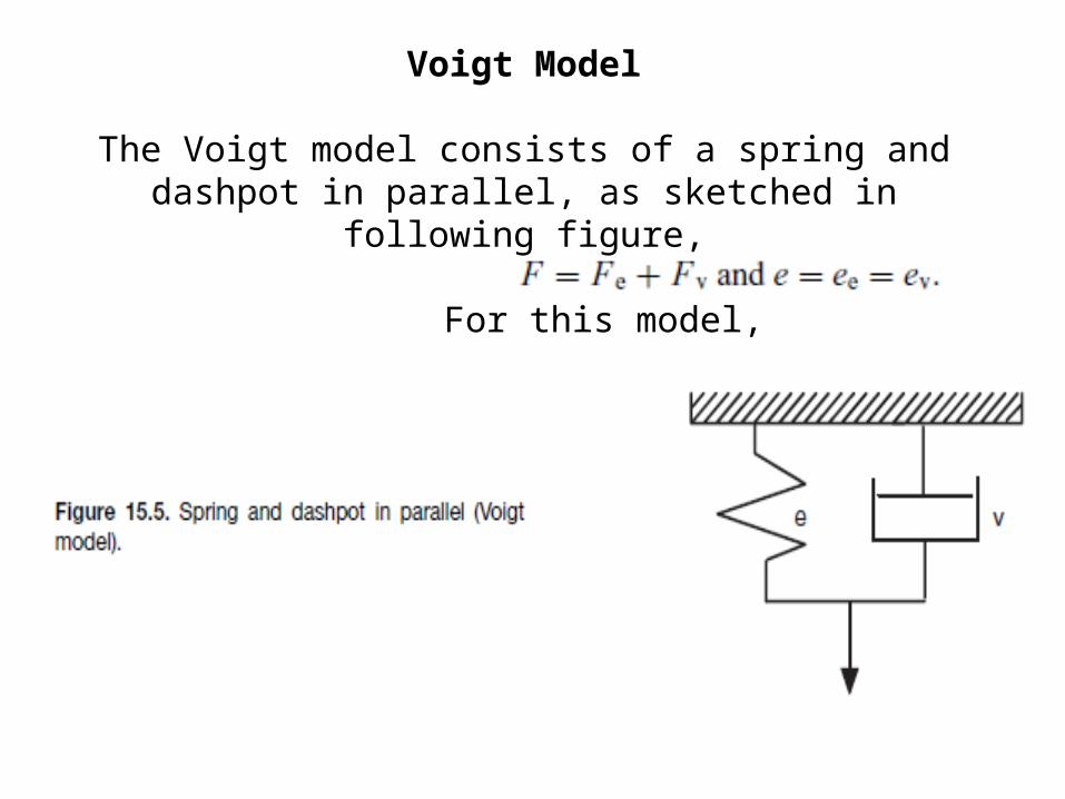
Voigt Model

The Voigt model consists of a spring and dashpot in parallel, as sketched in following figure,

For this model,

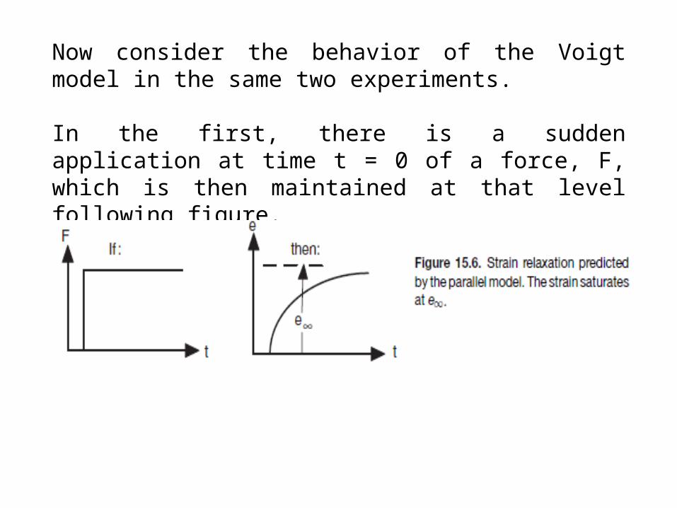
Now consider the behavior of the Voigt model in the same two experiments.

In the first, there is a sudden application at time t = 0 of a force, F, which is then maintained at that level following figure.

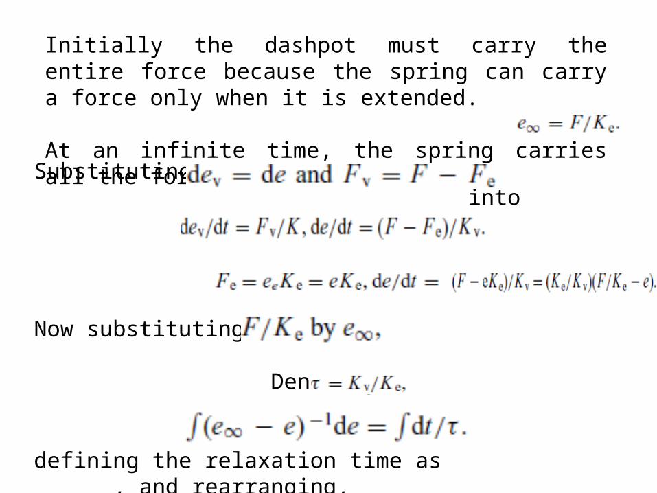
Initially the dashpot must carry the entire force because the spring can carry a force only when it is extended.

At an infinite time, the spring carries all the force, so

Substituting into

Now substituting

Denoting

defining the relaxation time as , and rearranging,

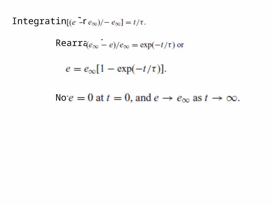
Integrating ln

Rearranging,

Note that

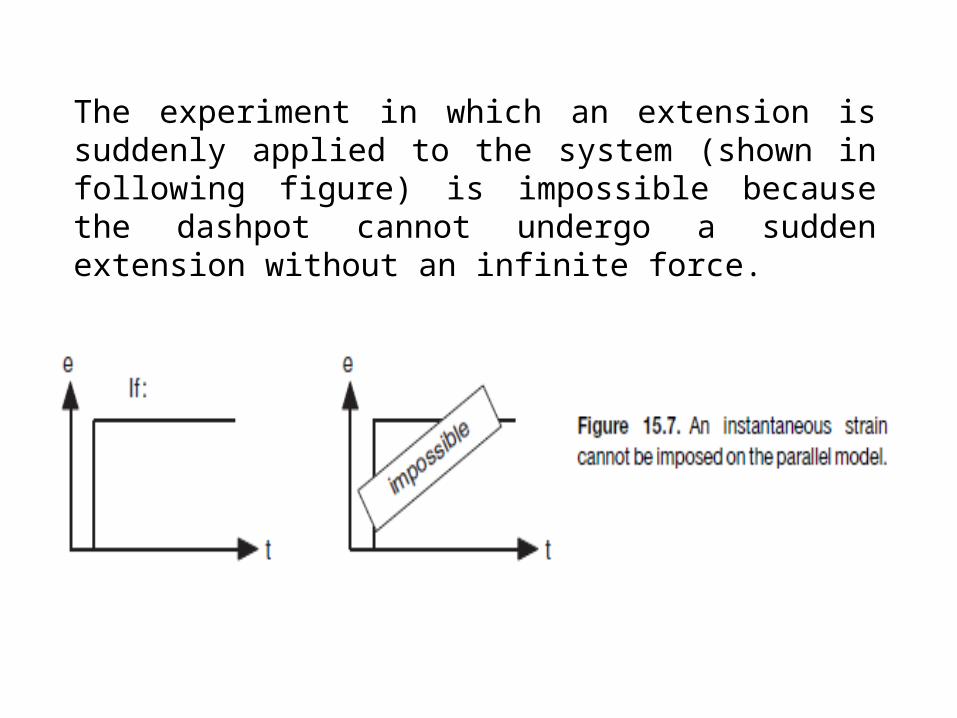
The experiment in which an extension is suddenly applied to the system (shown in following figure) is impossible because the dashpot cannot undergo a sudden extension without an infinite force.

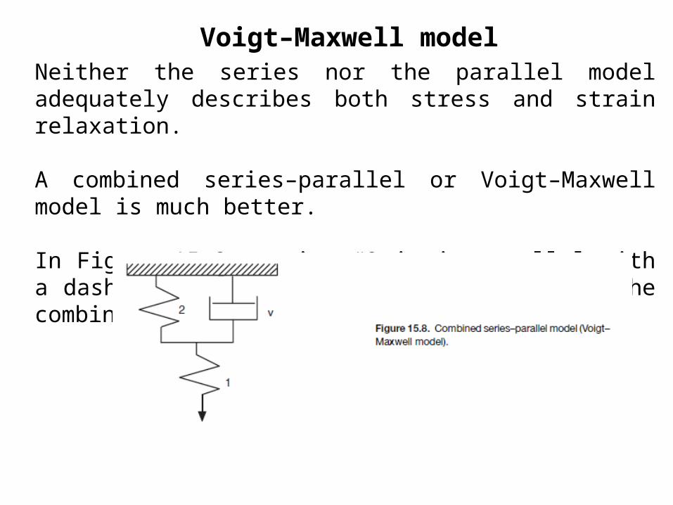
Neither the series nor the parallel model adequately describes both stress and strain relaxation.

A combined series–parallel or Voigt–Maxwell model is much better.

In Figure 15.8, spring #2 is in parallel with a dashpot and spring #1 is in series with the combination.

The basic equations of this model are F = F1 = F2 + Fv, ev = e2, and e = e1= e2.

Voigt–Maxwell model

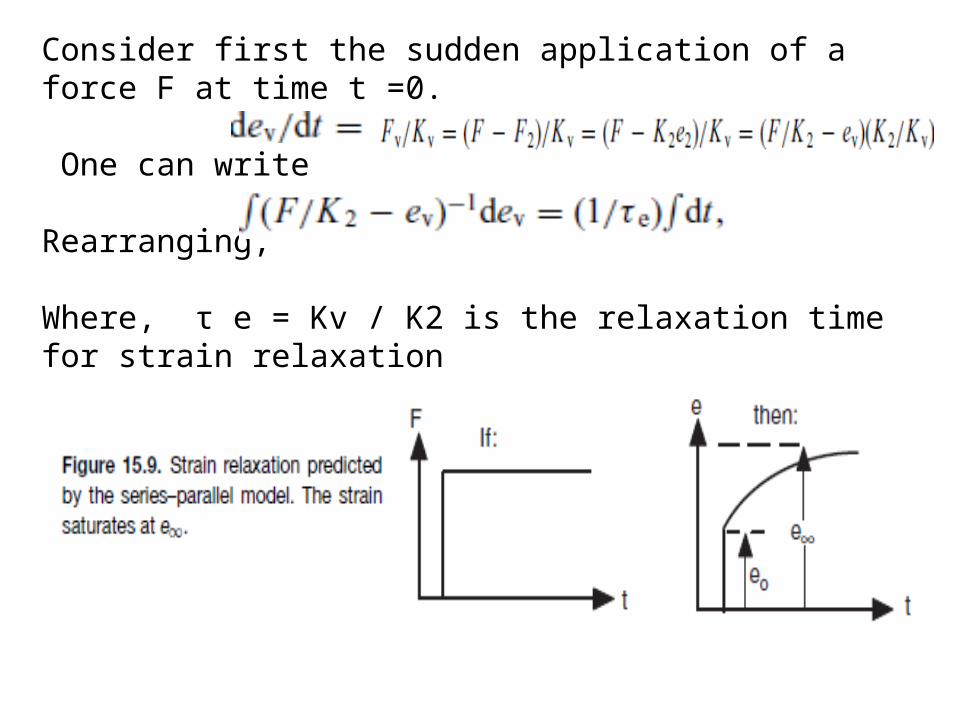
Consider first the sudden application of a force F at time t =0.

One can write Rearranging,

Where, τ e = Kv / K2 is the relaxation time for strain relaxation (see in following figure)

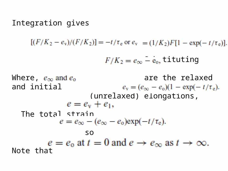
Integration gives

ln

Substituting

Where, are the relaxed and initial (unrelaxed) elongations,

The total strain so

Note that

Now consider the experiment in which an elongation, e, is suddenly imposed on the material.

Immediately after stretching, all of the strain occurs in spring 1, so e = F/K1, and thus the initial force Fo = eK1 (as shown in following figure).

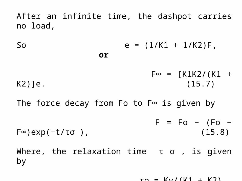
After an infinite time, the dashpot carries no load,

So e = (1/K1 + 1/K2)F, or

F∞ = [K1K2/(K1 + K2)]e. (15.7)

The force decay from Fo to F∞ is given by F = Fo − (Fo − F∞)exp(−t/τσ ), (15.8)

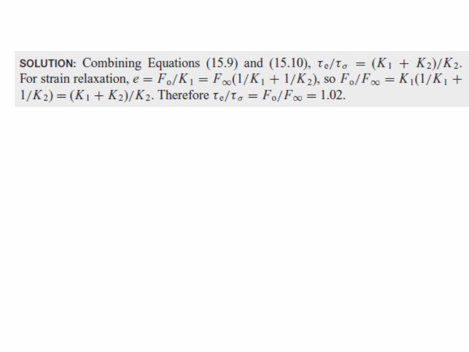
Where, the relaxation time τ σ , is given by τσ = Kv/(K1 + K2). (15.9)

Note that the relaxation time for stress relaxation is shorter than the relaxation time for strain relaxation, τe = Kv/K2. (15.10)

More complex models

More complicated models may be constructed using more spring and dashpot elements or elements with nonlinear behavior.

Nonlinear elasticity can be modeled by a nonlinear spring for which F = Ke f (e).

Non-Newtonian viscous behavior can be modeled by a nonlinear dashpot for which F = Kv f ( ˙e).

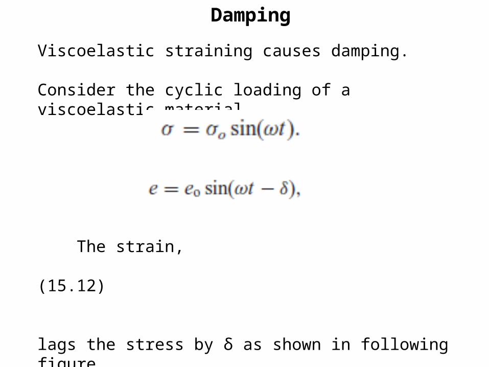
Damping

Viscoelastic straining causes damping.

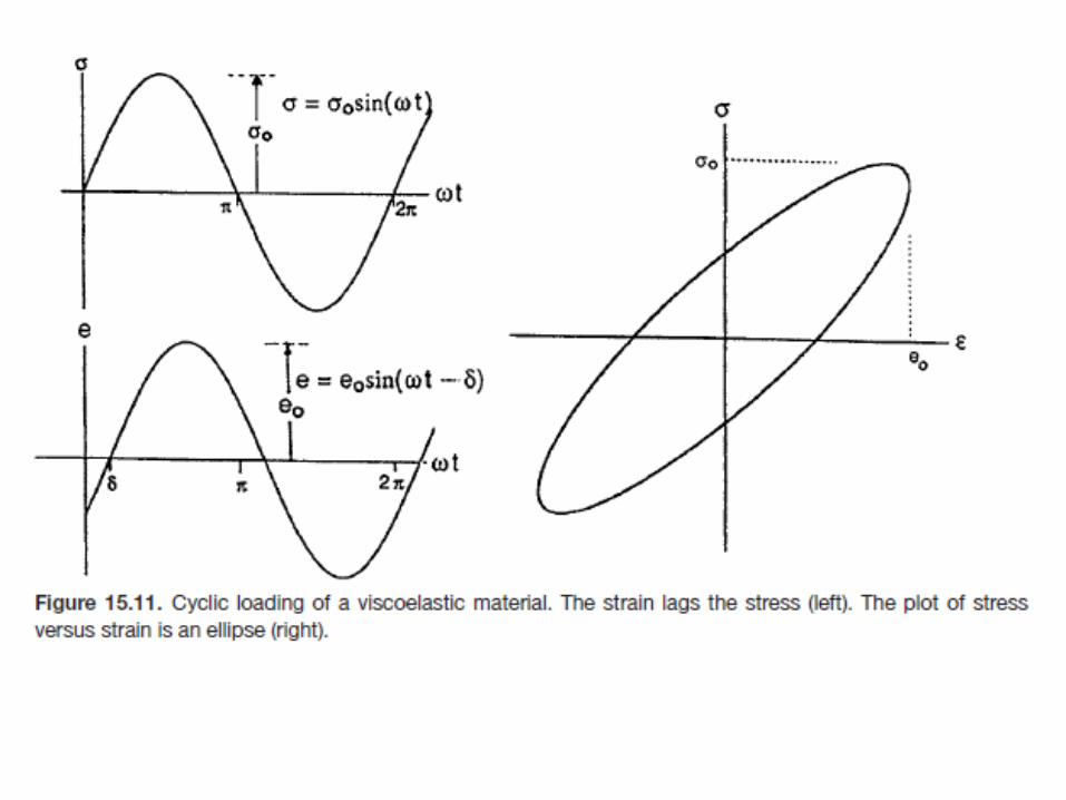
Consider the cyclic loading of a viscoelastic material,

(15.11)

The strain, (15.12)

lags the stress by δ as shown in following figure.

A plot of stress versus strain is an ellipse.

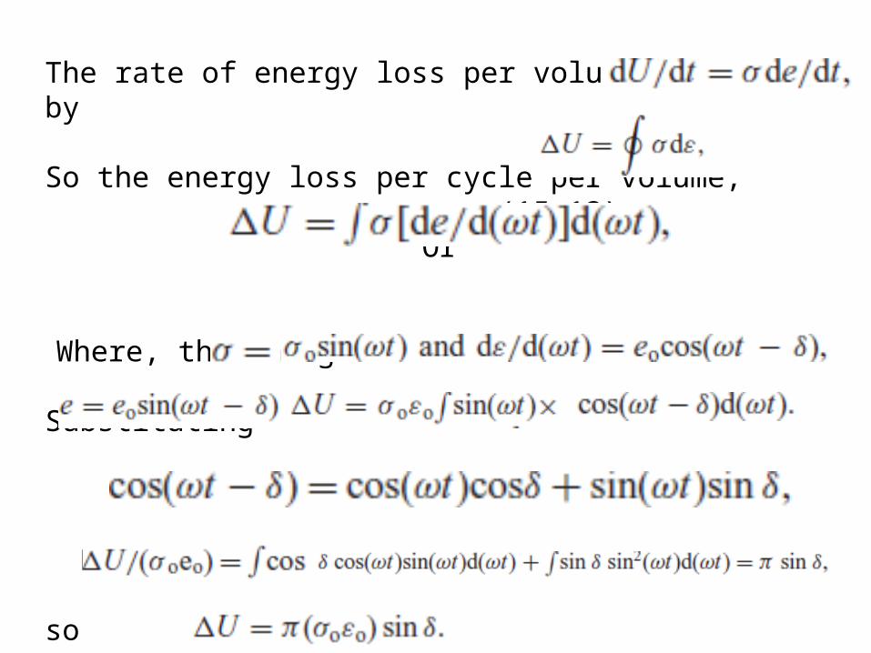
The rate of energy loss per volume is given by

So the energy loss per cycle per volume, (15.13)

Or

Where, the integration limits are 0 and 2π.

Substituting

But

so

Or (15.14)

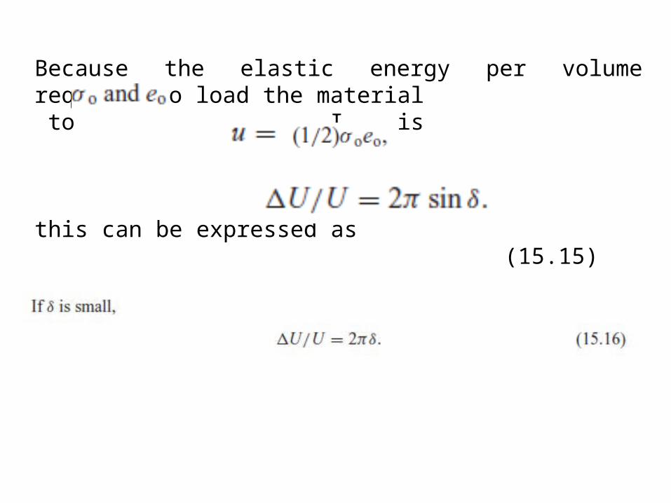
Because the elastic energy per volume required to load the material to I is

this can be expressed as (15.15)

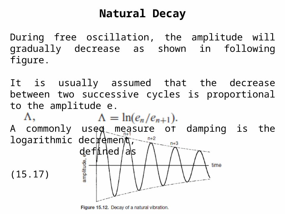
Natural Decay

During free oscillation, the amplitude will gradually decrease as shown in following figure. It is usually assumed that the decrease between two successive cycles is proportional to the amplitude e.

A commonly used measure of damping is the logarithmic decrement, defined as (15.17)

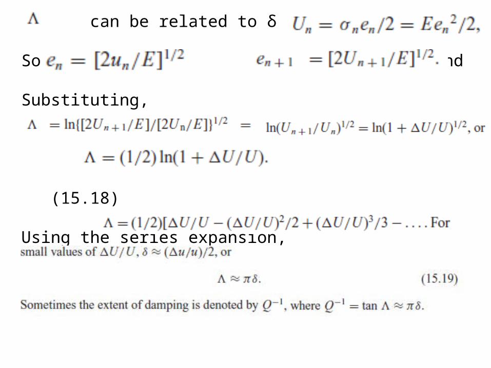
can be related to δ by recalling that

So and

Substituting,

(15.18)

Using the series expansion,

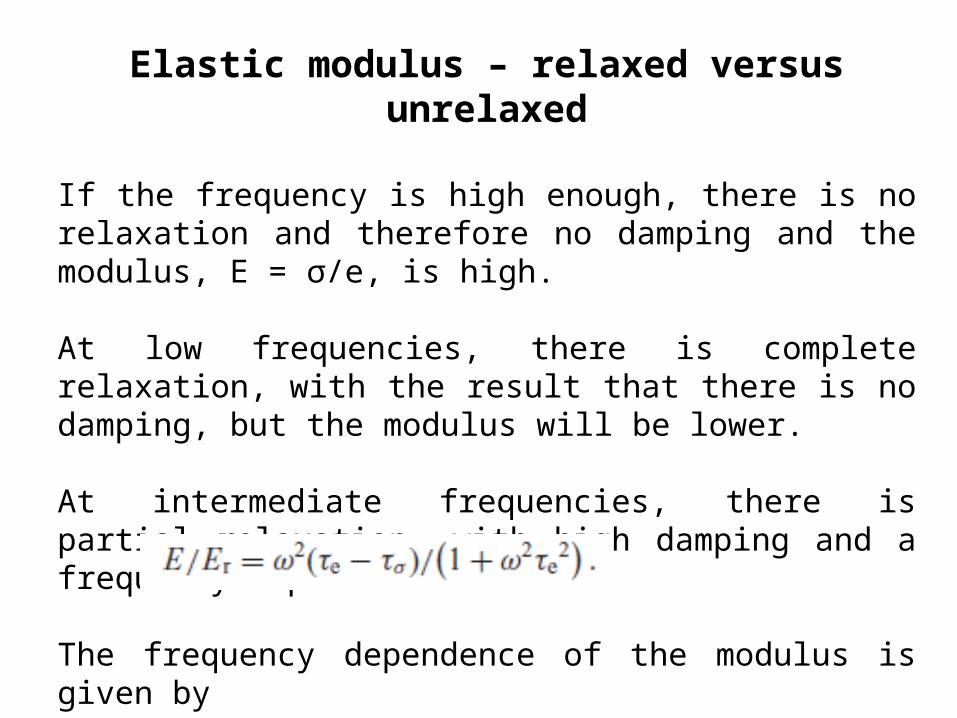
Elastic modulus – relaxed versus unrelaxed

If the frequency is high enough, there is no relaxation and therefore no damping and the modulus, E = σ/e, is high.

At low frequencies, there is complete relaxation, with the result that there is no damping, but the modulus will be lower.

At intermediate frequencies, there is partial relaxation, with high damping and a frequency-dependent modulus.

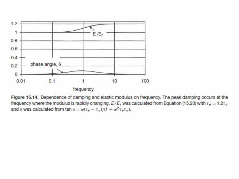
The frequency dependence of the modulus is given by

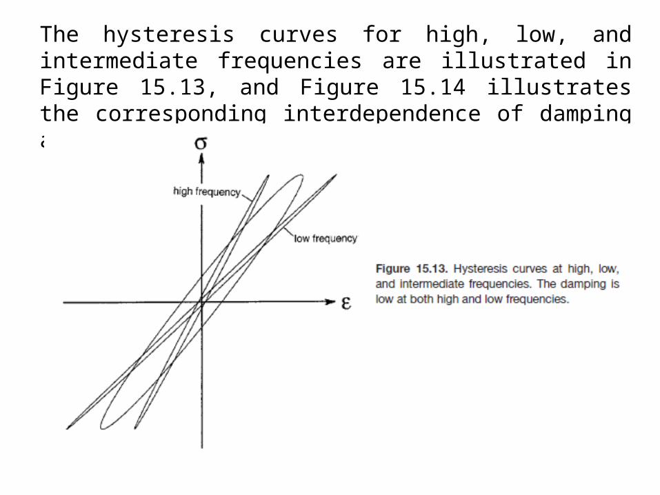
The hysteresis curves for high, low, and intermediate frequencies are illustrated in Figure 15.13, and Figure 15.14 illustrates the corresponding interdependence of damping and modulus.

Thermo - elastic Effect

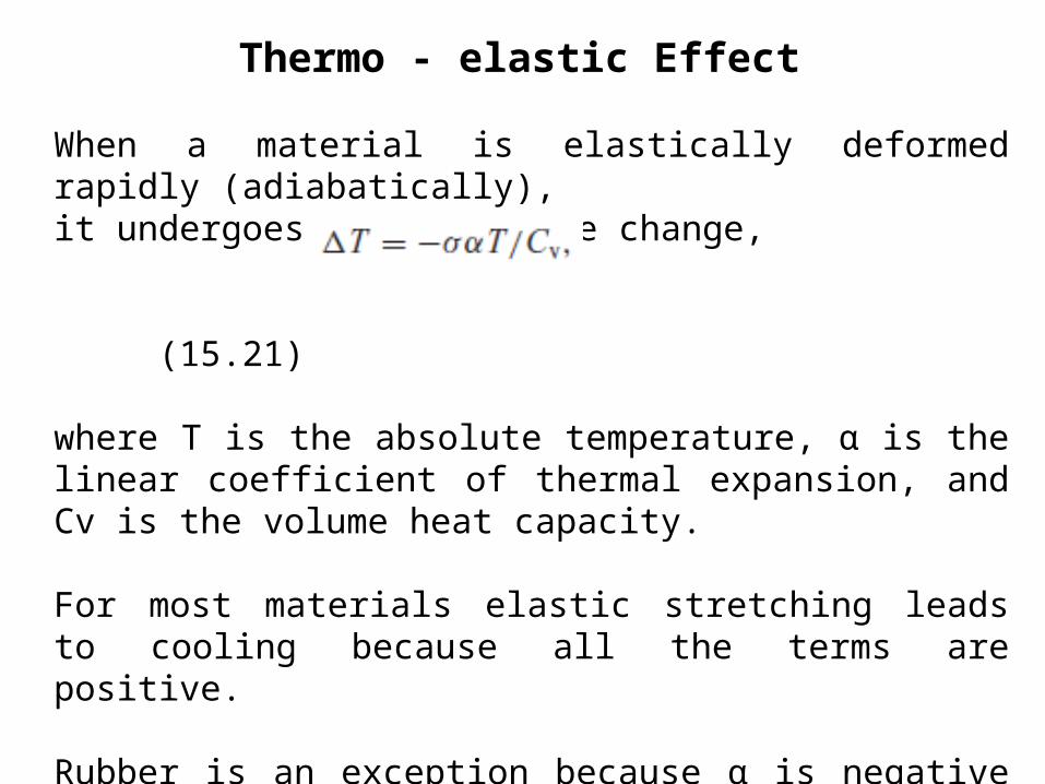
When a material is elastically deformed rapidly (adiabatically), it undergoes a temperature change, (15.21)

where T is the absolute temperature, α is the linear coefficient of thermal expansion, and Cv is the volume heat capacity.

For most materials elastic stretching leads to cooling because all the terms are positive.

Rubber is an exception because α is negative when it is under tension.

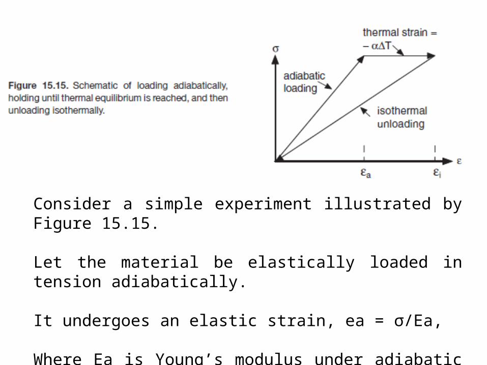
Consider a simple experiment illustrated by Figure 15.15.

Let the material be elastically loaded in tension adiabatically.

It undergoes an elastic strain, ea = σ/Ea,

Where Ea is Young’s modulus under adiabatic conditions.

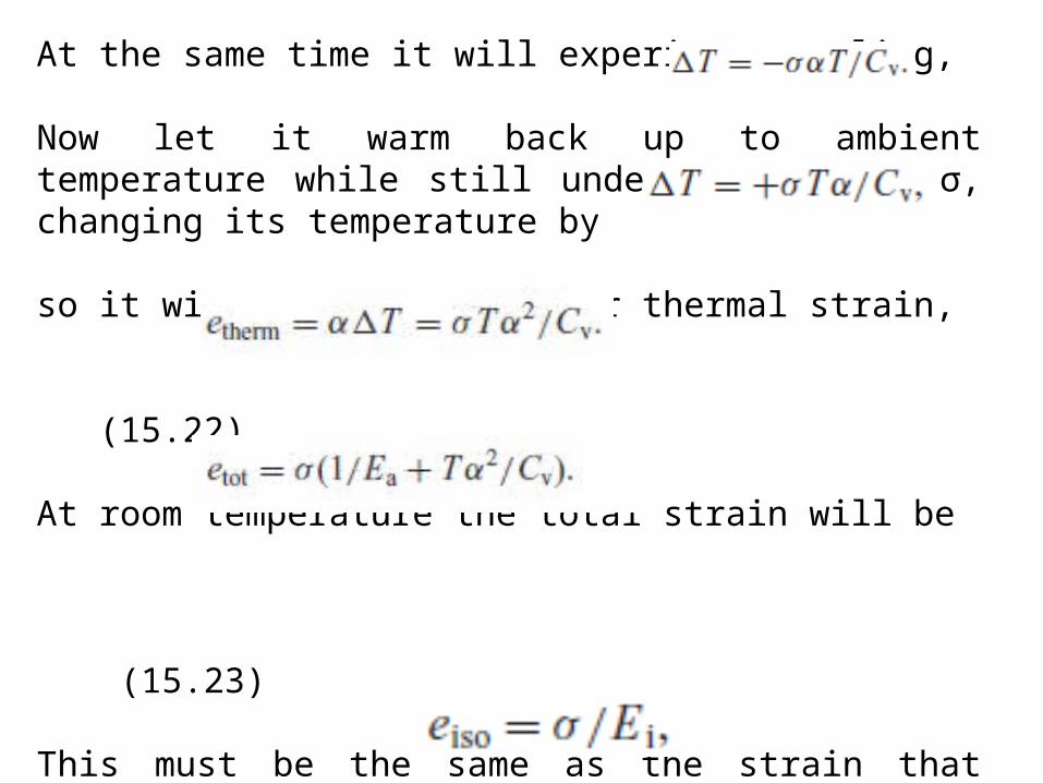
At the same time it will experience cooling,

Now let it warm back up to ambient temperature while still under the stress σ, changing its temperature by

so it will undergo a further thermal strain, (15.22)

At room temperature the total strain will be

(15.23)

This must be the same as the strain that would have resulted from stressing the material isothermally (so slowly that it remained at room temperature),

so

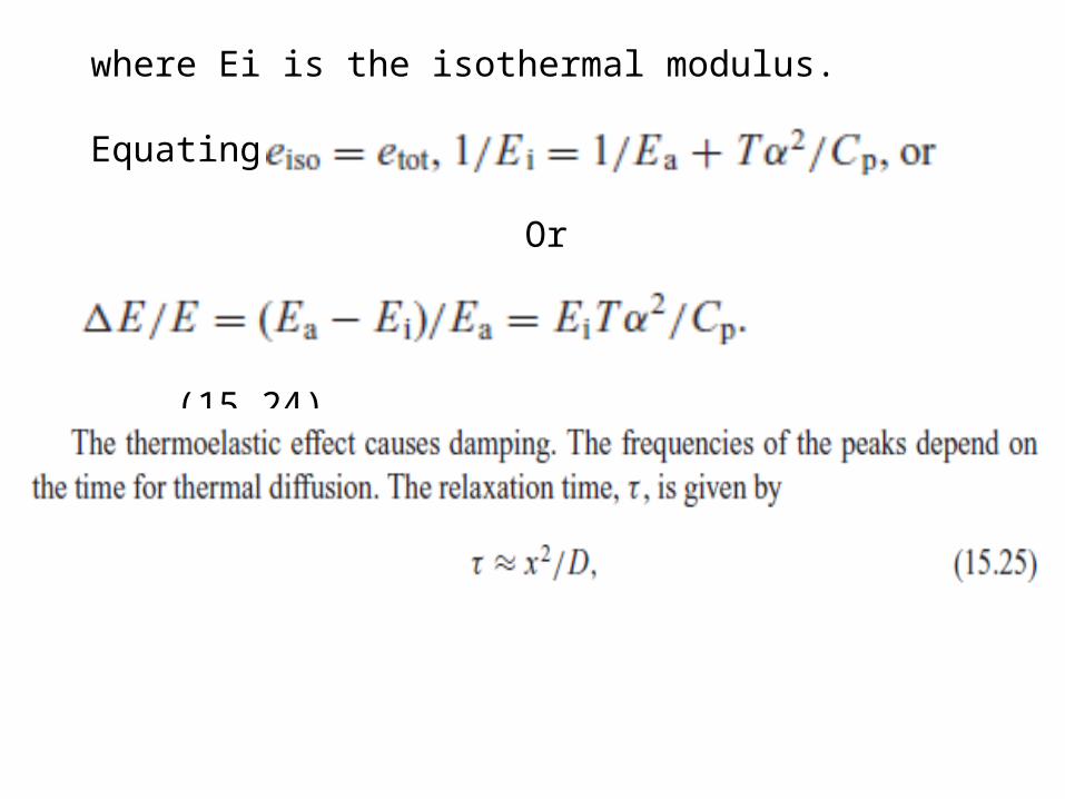
where Ei is the isothermal modulus.

Equating

Or (15.24)

where x is the thermal diffusion distance and D is the thermal diffusivity.

The relaxation time, τ , and therefore the frequencies of the damping peaks depend strongly on the diffusion distance, x.

There are thermal currents in a polycrystal between grains of different orientations because of their different elastic responses.

In this case the diffusion distance, x, is comparable to the grain size, d.

For specimens in bending, there are also thermal currents from one side of the specimen to the other.

These cause damping peaks with a diffusion distance x comparable to the specimen size.

Elastic behavior

Elastic strains in metals and ceramics occur by stretching of primary metallic, covalent, or ionic bonds.

The elastic modulus of most crystals varies with direction by less than a factor of 3.

The effects of alloying, and of thermal and mechanical treatments on the elastic module of crystals are relatively small.

As the temperature is increased from absolute zero to the melting point, Young’s modulus usually decreases by a factor of no more than 5.

For polymers, however, a temperature change of 30◦C may change the elastic modulus by a factor of 1000. 345

Elastic deformation of polymers involves stretching of the weak van der Waals bonds between neighboring molecular chains and rotation of covalent bonds.

This accounts for the fact that the elastic module of random linear polymers are often at least two orders of magnitude lower than those of metals and ceramics.

However, highly oriented polymers may have Young’s module that are higher than those of the stiffest metals when they are tested parallel to the direction of chain alignment.

Figure 20.1 is a schematic plot showing how E increases with the fraction of covalent bonds aligned with the loading direction.

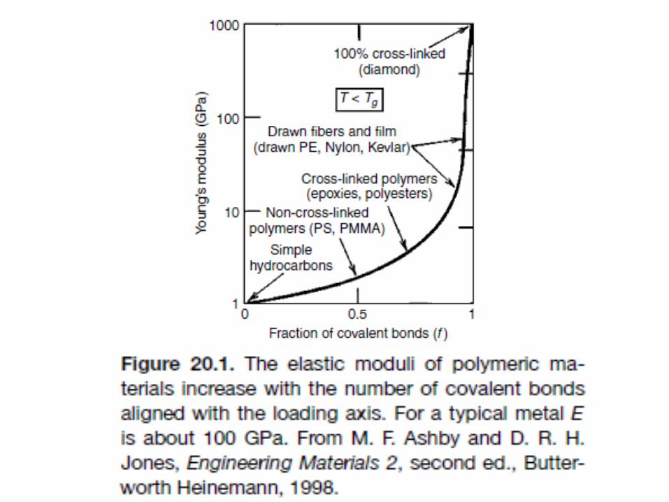
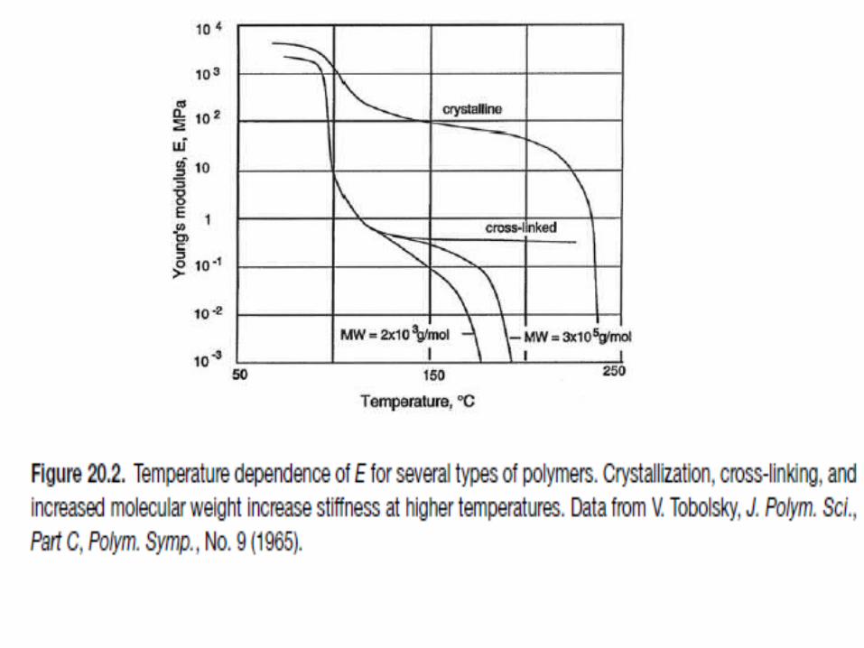
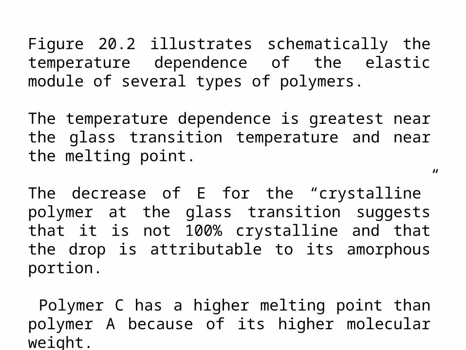
Figure 20.2 illustrates schematically the temperature dependence of the elastic module of several types of polymers.

The temperature dependence is greatest near the glass transition temperature and near the melting point.

The decrease of E for the “crystalline” polymer at the glass transition suggests that it is not 100% crystalline and that the drop is attributable to its amorphous portion.

Polymer C has a higher melting point than polymer A because of its higher molecular weight.

The cross-linked polymer cannot melt without breaking the covalent bonds in the cross-links.

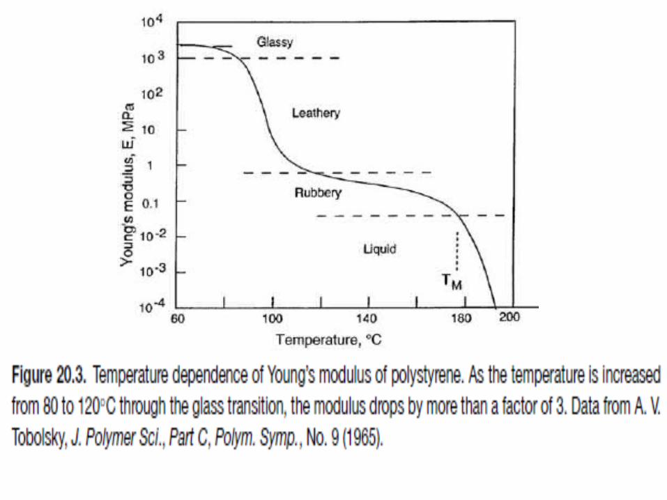
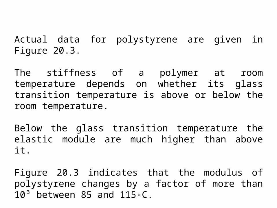
Actual data for polystyrene are given in Figure 20.3.

The stiffness of a polymer at room temperature depends on whether its glass transition temperature is above or below the room temperature.

Below the glass transition temperature the elastic module are much higher than above it.

Figure 20.3 indicates that the modulus of polystyrene changes by a factor of more than 10³ between 85 and 115◦C.

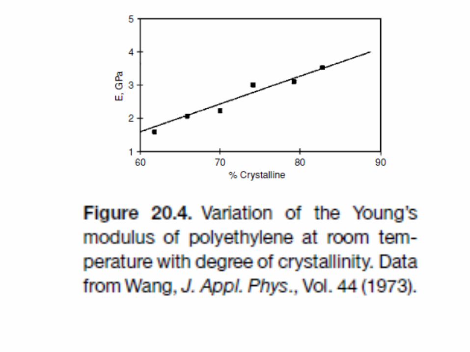
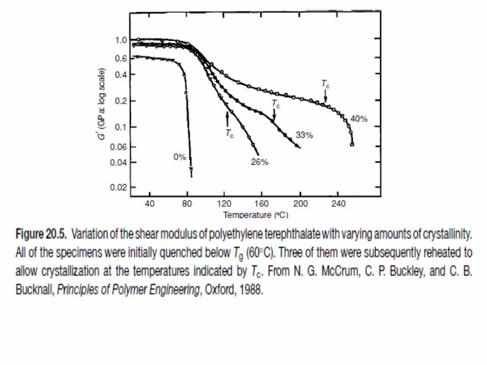
The elastic module of thermoplastics increase with the degree of crystallinity as shown in Figures 20.4 and 20.5.

A strong time (and therefore strain-rate) dependence of the elastic modulus accompanies the strong temperature dependence as shown in Figure 20.6.

This is because polymers undergo time-dependent viscoelastic deformation when stressed.

If a stress is suddenly applied, there is an immediate elastic response.

More deformation occurs with increasing time.

The effect is so large near the glass transition temperature that it is customary to define the modulus in terms of the time of loading.

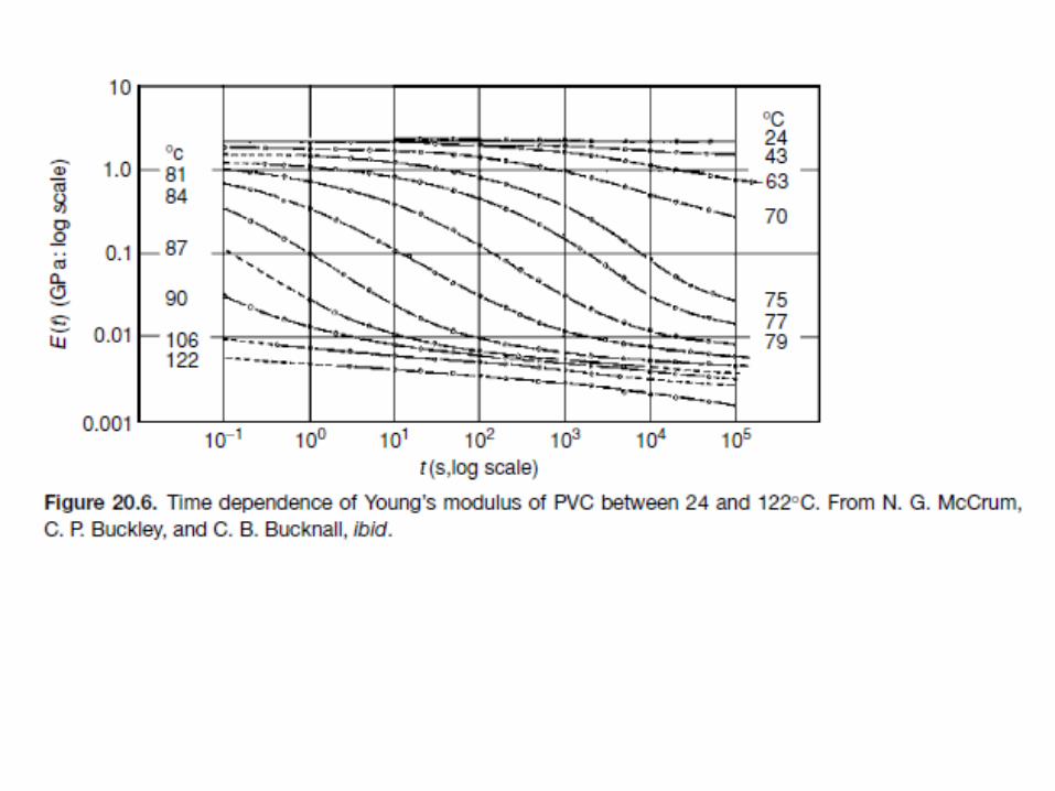
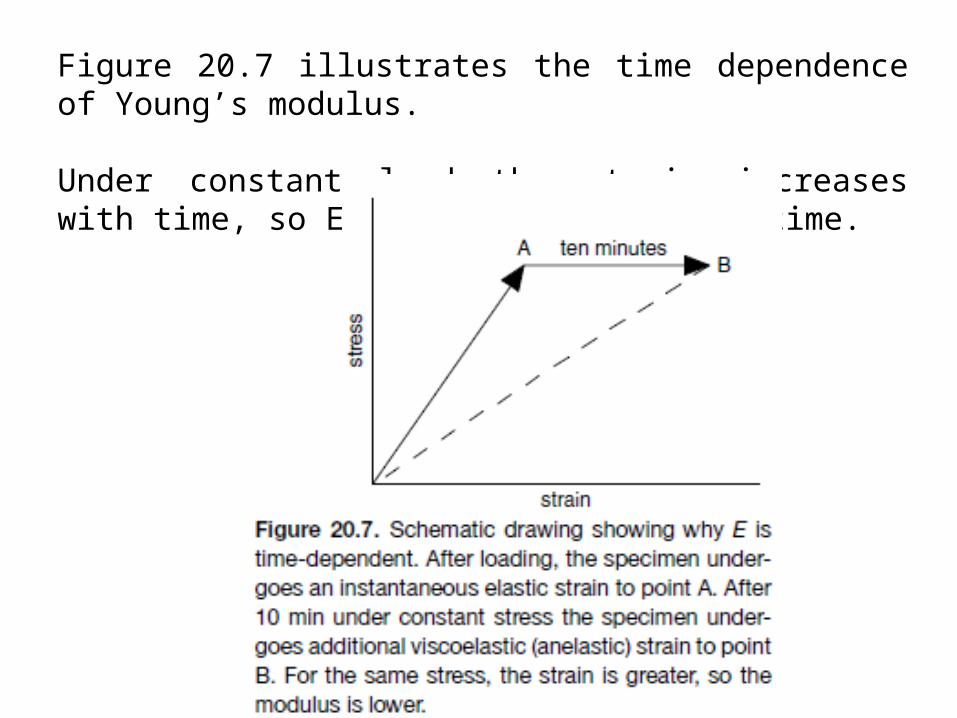
Figure 20.7 illustrates the time dependence of Young’s modulus.

Under constant load the strain increases with time, so E = σ/ε decreases with time.

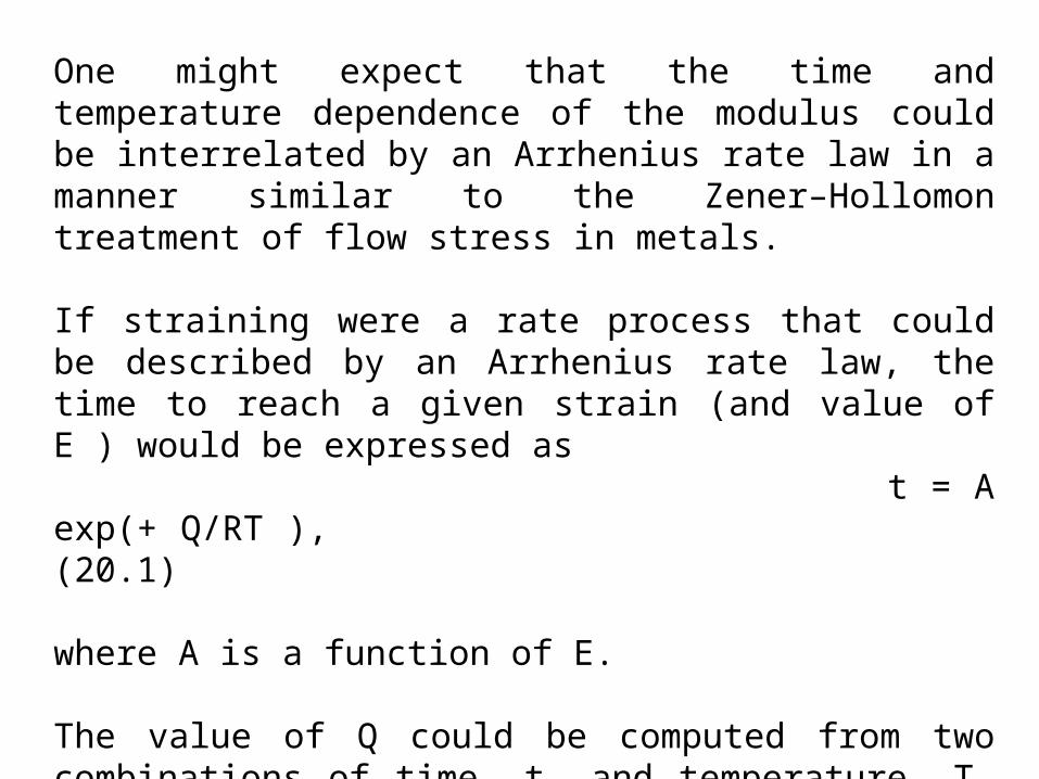
One might expect that the time and temperature dependence of the modulus could be interrelated by an Arrhenius rate law in a manner similar to the Zener–Hollomon treatment of flow stress in metals.

If straining were a rate process that could be described by an Arrhenius rate law, the time to reach a given strain (and value of E ) would be expressed as t = A exp(+ Q/RT ), (20.1)

where A is a function of E.

The value of Q could be computed from two combinations of time, t, and temperature, T, that give the same value of E.

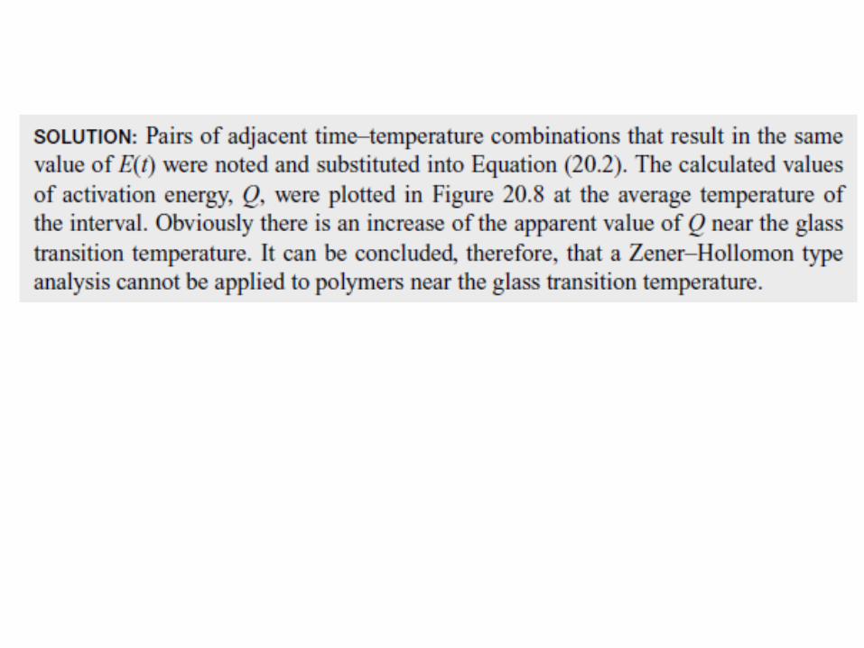
In that case t1/t2 = exp[(Q/R)(1/T1 − 1/T2)], so Q = R ln(t1/t2)/(1/T1 − 1/T2). (20.2)

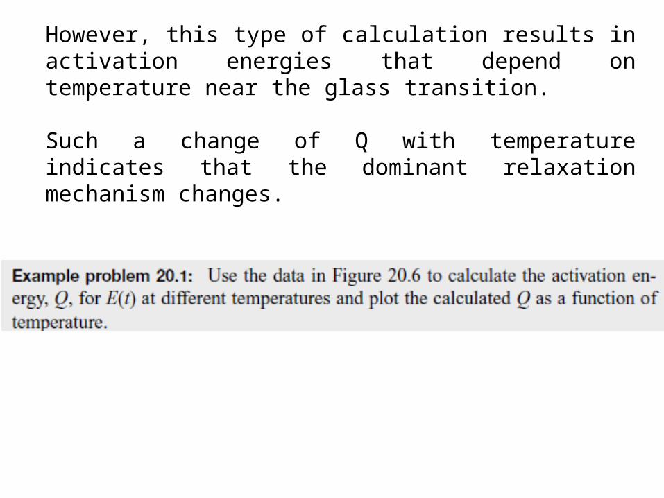
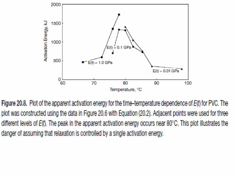
However, this type of calculation results in activation energies that depend on temperature near the glass transition.

Such a change of Q with temperature indicates that the dominant relaxation mechanism changes.

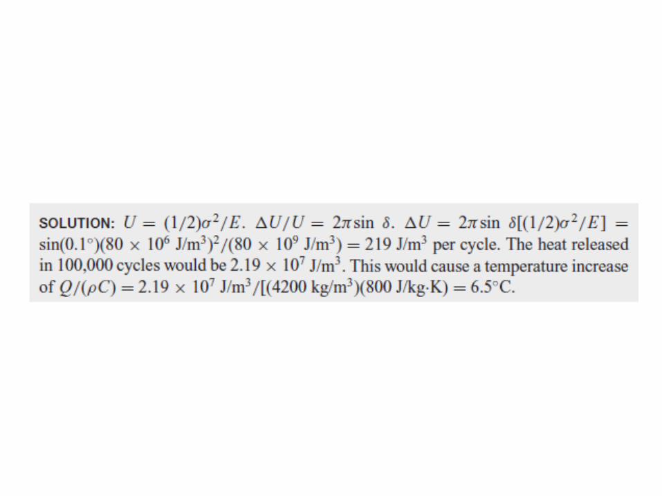
Example Problem 20.1 and Figure 20.8 illustrates this.

Examination of the curves for E(t) versus log(t) at different temperatures in Figure 20.6 indicates that they all have similar shapes.

The curve for one temperature can be generated from that at another temperature by simply shifting it in time by a constant shift factor, log(a) = log(t2) − log(t1) = log(t2/t1).

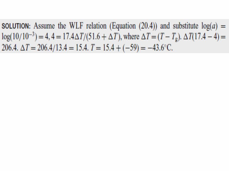
Williams, Landel, and Ferry proposed that the shift factor needed to bring the curve for temperature, T, into coincidence with that for a reference temperature, Ts, could be expressed as log(a) = C1(T − Ts)/[C2 + (T − Ts)], (20.3)

where C1 and C2 are constants. This empirical equation works very well near the glass transition temperature.

If the reference temperature is taken as the glass transition temperature, Ts = Tg, log(a) = C1g(T − Tg)/[C2g + (T − Tg)]. (20.4)

It was suggested that values of about C1g = 17.4 and C2g = 51.6 K are appropriate for many polymers.

Rubber Elasticity

The elastic behavior of rubber is very different from that of crystalline materials.

Rubber is a flexible polymer in which the molecular chains are cross-linked.

The number of crosslinks is controlled by the amount of cross-linking agent compounded with the rubber.

Elastic extension occurs by straightening of the chain segments between the cross-links.

With more cross-linking, the chain segments are shorter and have less freedom of motion, so the rubber is stiffer.

Originally only sulfur was used for cross-linking, but today other cross-linking agents are used.

Under a tensile stress the end-to-end lengths of the segments increase, but thermal vibrations of the free segments tend to pull the ends together, just as the tension in violin strings is increased by their vibration.

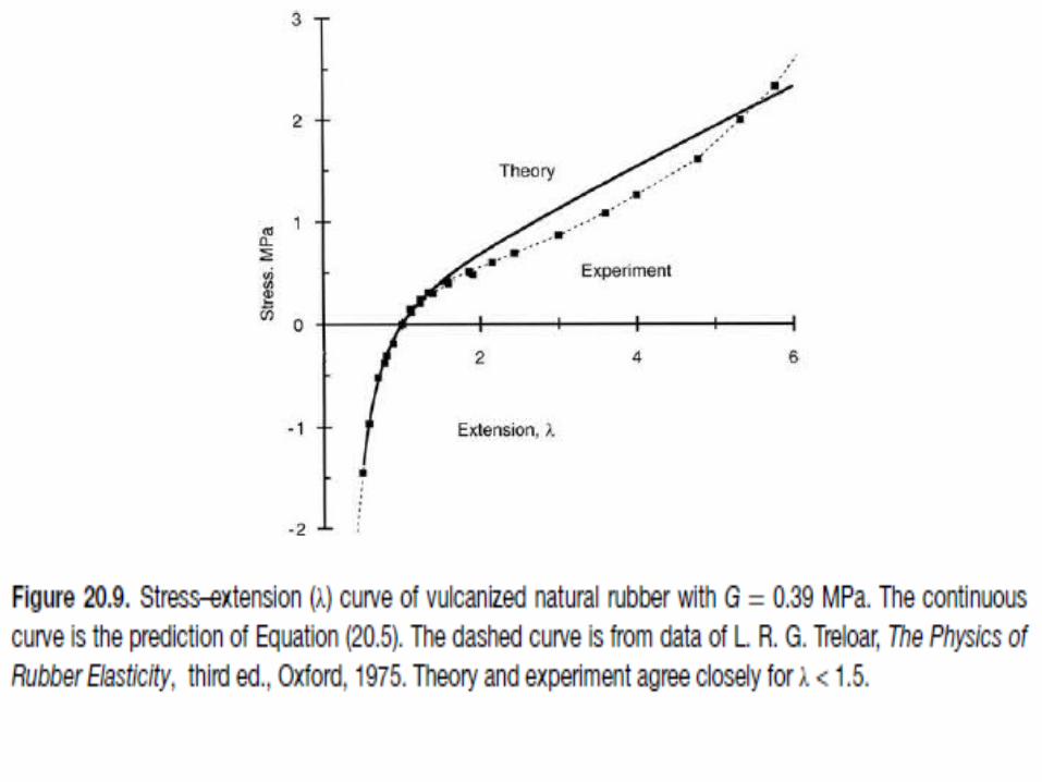
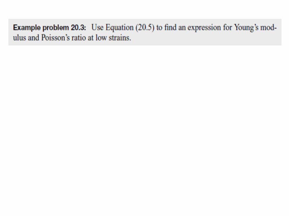
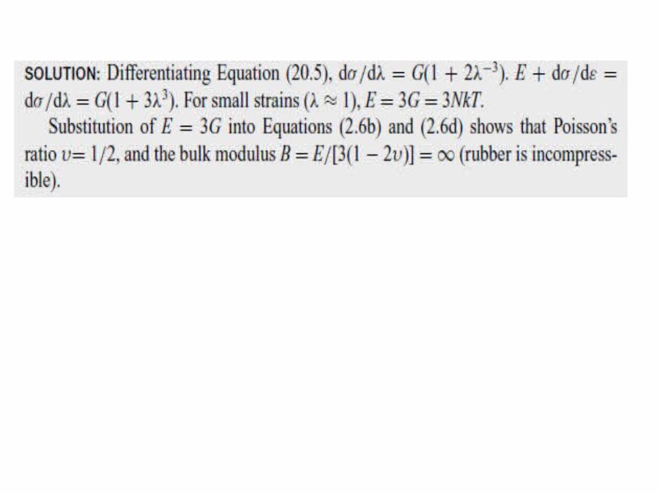
A mathematical model that describes the elastic response under uniaxial tension or compression predicts that σ = G(λ − 1/λ2), (20.5)

where λ is the extension ratio, λ = L/Lo = 1 + e, where e is the engineering strain.

The shear modulus, G, depends on the temperature and on the length of the free segments, G = NkT, (20.6)where N is the number of chain segments/volume and k is Boltzmann’s constant.

Figure 20.9 shows the theoretical predictions of equation with σ normalized by G.

Agreement with experiment is very good for λ < 1.5, but is poorer at higher values of λ.

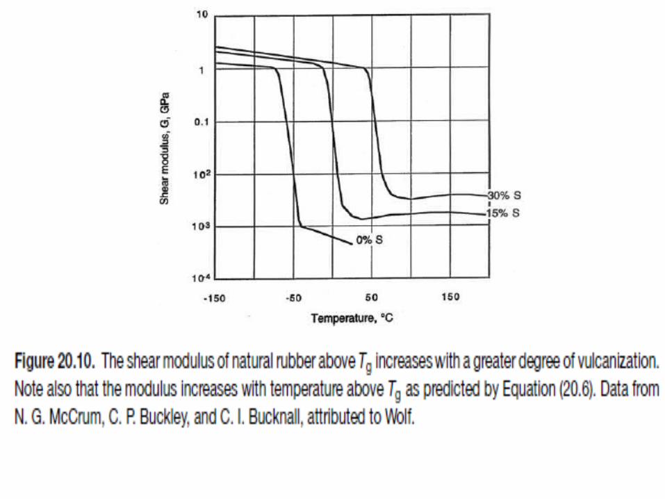
Note that because G = NkT, the elastic modulus increases with temperature in the rubbery range above the glass transition temperature (see Figure 20.10).

The increase of modulus with increasing sulfur content is attributable to the greater number of crosslinks, N.

The negative thermal expansion coefficient under tension can be demonstrated by stretching a rubber band by hanging a fixed weight (constant σ) on it so that λ > 1 and then heating it with a hair dryer.

The weight will rise as the rubber band contracts.

Damping

The viscoelastic behavior that is responsible for the time and temperature dependence of the modulus also causes damping.

The two phenomena are interrelated.

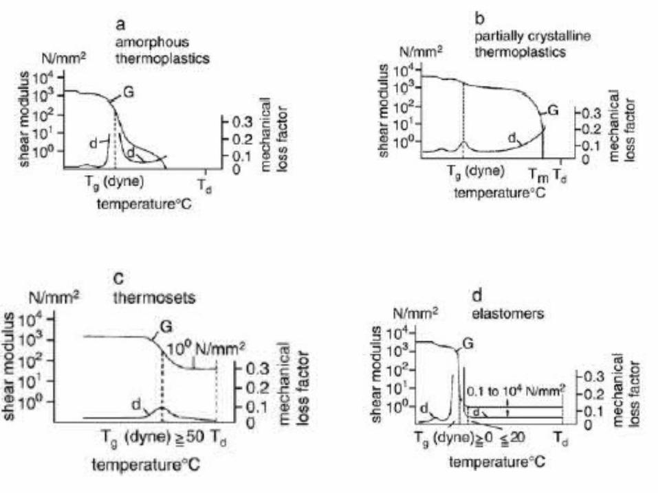
Figure 20.12 shows schematically that the damping is greatest in the temperature range in which the decrease of modulus with temperature, −dE/dT, is greatest.

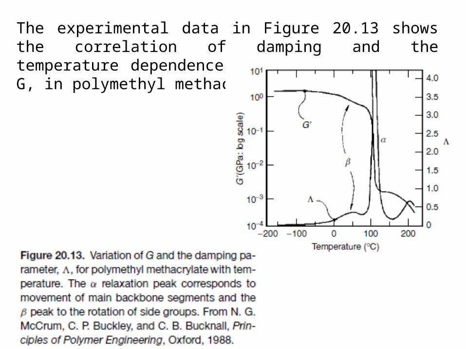
The experimental data in Figure 20.13 shows the correlation of damping and the temperature dependence of the shear modulus, G, in polymethyl methacrylate.

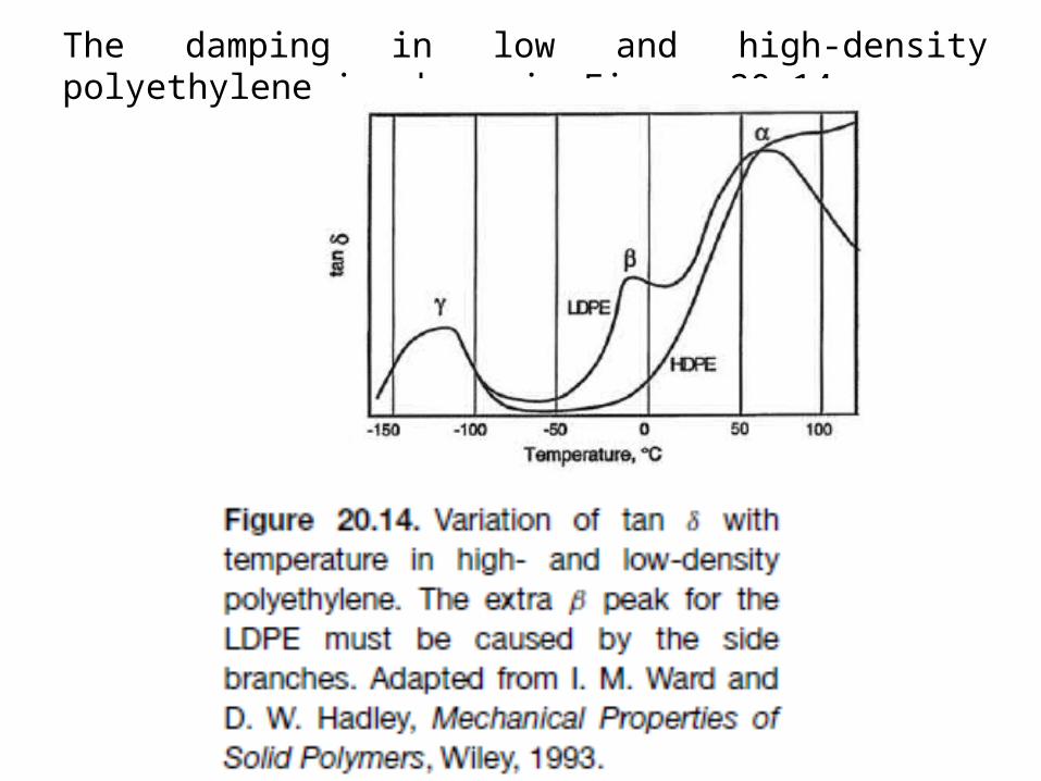
The damping in low and high-density polyethylene is shown in Figure 20.14.

Mechanical hysteresis is the energy loss per volume per cycle.

The area under the loading curve represents the mechanical energy per volume put into the material during loading, whereas the area under the unloading curve represents the mechanical energy recovered during unloading.

The area between the two curves is the magnitude of the hysteresis and represents the energy that remains in the material, which is almost entirely converted to heat.

Yielding

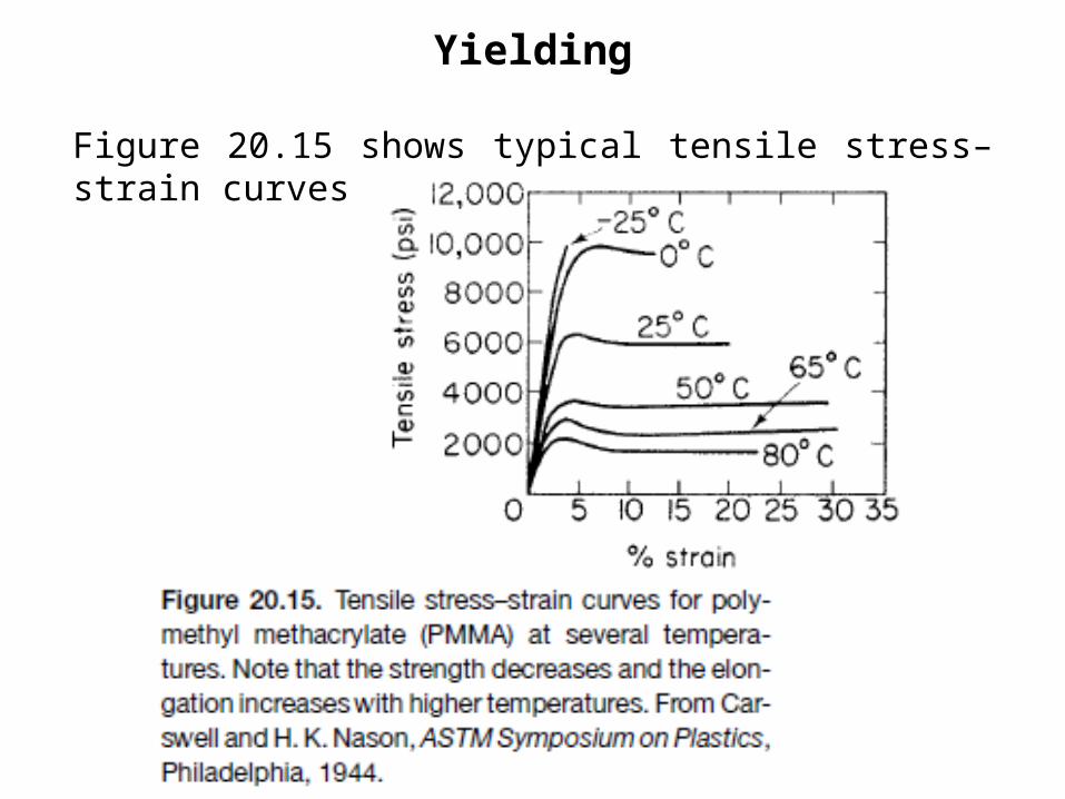
Figure 20.15 shows typical tensile stress–strain curves for a thermoplastic.

The lower strengths at higher temperatures are obvious. Increased strain rates have the same effect as decreased temperatures.

At low temperatures PMMA is brittle. At higher temperatures, the initial elastic region is followed by a drop in load that accompanies yielding.

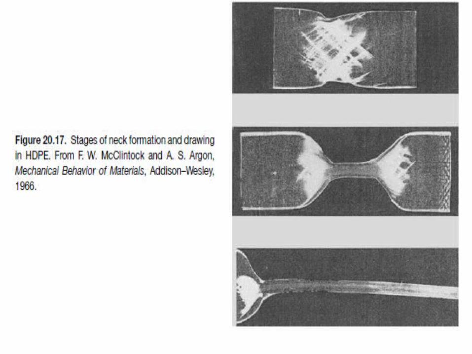
A strained region or neck forms and propagates the length of the tensile specimen (Figures 20.16 and 20.17).

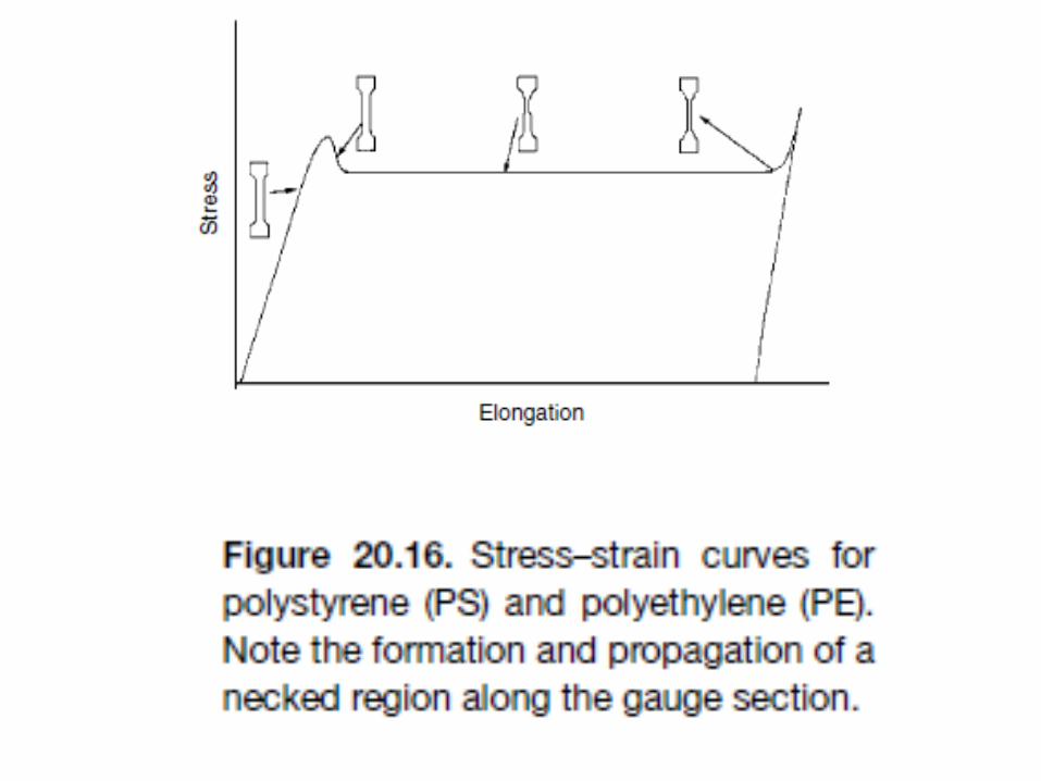
Only after the whole gauge section is strained does the stress again rise.

Superficially this is similar to the upper and lower yield points and propagation of L¨uder’s bands in low carbon steel after strain-aging.

However, there are several notable differences.

The engineering strain in the necked region of a polymer is several hundred percent, in contrast to one or two percent in a L¨uder’s band in steel.

Also, the mechanism is different.

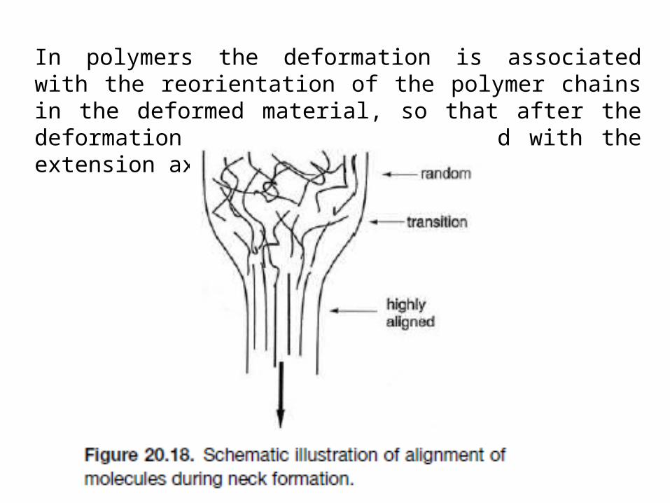
In polymers the deformation is associated with the reorientation of the polymer chains in the deformed material, so that after the deformation the chains are aligned with the extension axis (see Figure 20.18.)

This causes a very large increase in the elastic modulus.

Continued stretching, after the necked region has propagated the length of the gauge section, can be achieved only by continued elastic deformation.

This now involves opening of the bond angle of the C–C bonds.

The stress rises rapidly until the specimen fractures.

If the specimen is unloaded before fracture and a stress is applied perpendicular to the axis of prior extension, the material will fail at very low loads because only van der Waals bonds need be broken.

Polymers with low molecular weights may fail before necking.

Low molecular weights may result from the polymerization process or from environmental degradation.

Although high molecular weights tend to result in stronger and more ductile polymers, they also raise the viscosity of the molten polymer, which is often undesirable in injection molding.

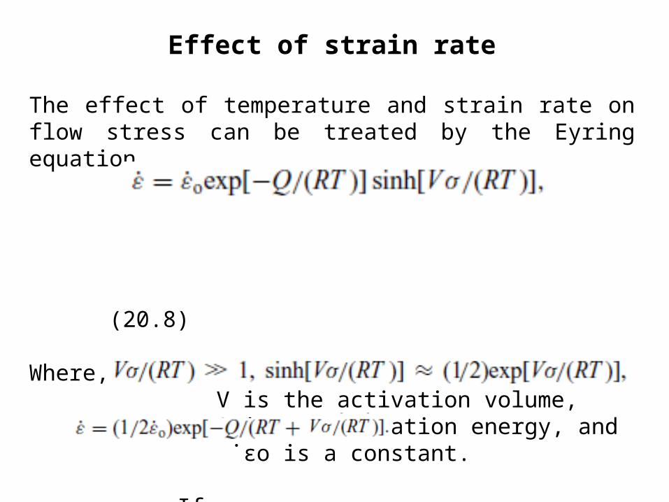
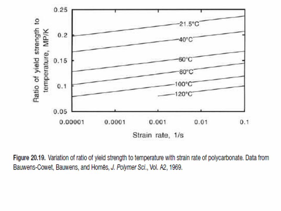
Effect of strain rate

The effect of temperature and strain rate on flow stress can be treated by the Eyring equation (20.8)

Where, V is the activation volume, Q is an activation energy, and ˙εo is a constant.

If

So

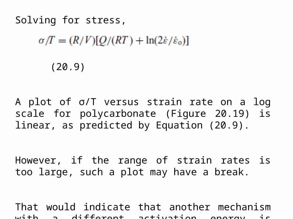
Solving for stress,

(20.9)

A plot of σ/T versus strain rate on a log scale for polycarbonate (Figure 20.19) is linear, as predicted by Equation (20.9).

However, if the range of strain rates is too large, such a plot may have a break.

That would indicate that another mechanism with a different activation energy is involved.

Crazing

Many thermoplastics undergo a phenomenon known as crazing when loaded in tension.

Sometimes the term craze yielding is used to distinguish this from the usual shear yielding.

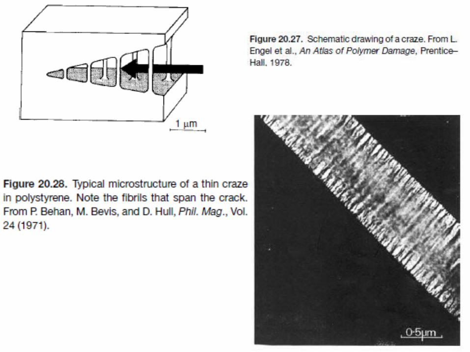
A craze is an opening resembling a crack. However, a craze is not a crack in the usual sense.

Voids form and elongate in the direction of extension. As a craze advances, fibers span the opening, linking the two halves.

Figure 20.27 is a schematic drawing of a craze and Figure 20.28 shows crazes in polystyrene.

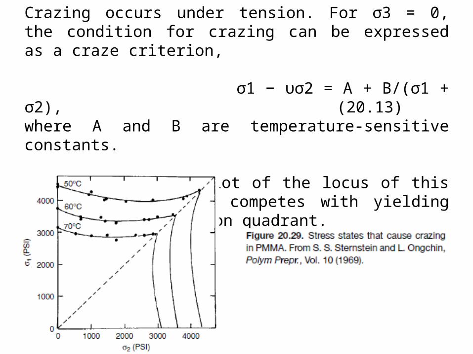
Crazing occurs under tension. For σ3 = 0, the condition for crazing can be expressed as a craze criterion,

σ1 − υσ2 = A + B/(σ1 + σ2), (20.13)where A and B are temperature-sensitive constants.

Figure 20.29 is a plot of the locus of this criterion. Crazing competes with yielding in the biaxial tension quadrant.

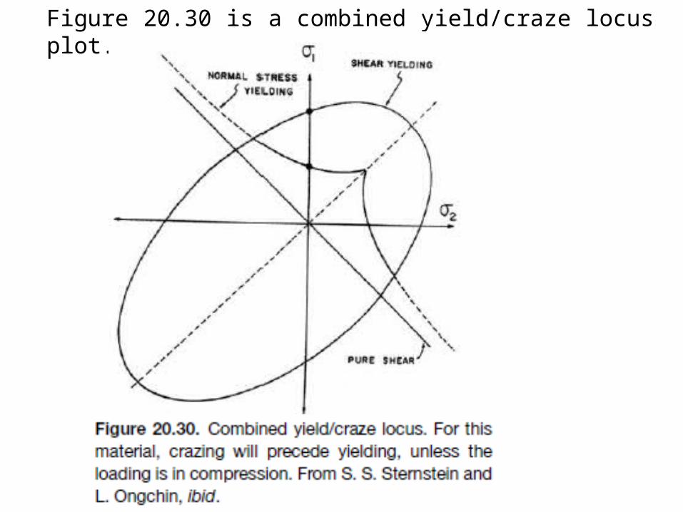
Figure 20.30 is a combined yield/craze locus plot.

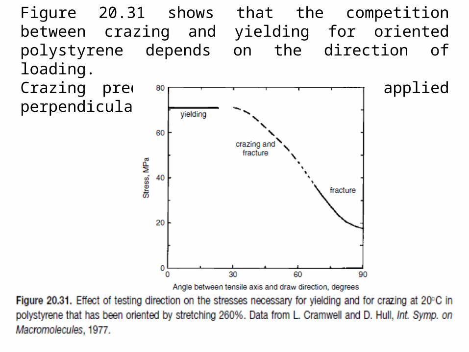
Figure 20.31 shows that the competition between crazing and yielding for oriented polystyrene depends on the direction of loading. Crazing predominates if tension is applied perpendicular to the fiber alignment.