Embed Size (px)
Citation preview

Joaquim P. Marques de Sá
Chance

Joaquim P. Marques de Sá
CHANCE
The Life of Games&
the Game of Life
With 105 Figures and 10 Tables
123

Prof. Dr. Joaquim P. Marques de Sá
Original Portuguese edition © Gravida 2006
ISBN 978-3-540-74416-0 e-ISBN 978-3-540-74417-7
DOI 10.1007/978-3-540-74417-7
Library of Congress Control Number: 2007941508
© Springer-Verlag Berlin Heidelberg 2008
his work is subject to copyright. All rights are reserved, whether the whole or part of the material isconcerned, specifically the rights of translation, reprinting, reuse of illustrations, recitation, broad-casting, reproduction on microfilm or in any other way, and storage in data banks. Duplication ofthis publication or parts thereof is permitted only under the provisions of the German CopyrightLaw of September 9, 1965, in its current version, and permission for use must always be obtainedfrom Springer. Violations are liable for prosecution under the German Copyright Law.
he use of general descriptive names, registered names, trademarks, etc. in this publication does notimply, even in the absence of a specific statement, that such names are exempt from the relevantprotective laws and regulations and therefore free for general use.
Typesetting: LE-TEX Jelonek, Schmidt & Vöckler GbR, Leipzig, GermanyProduction: LE-TEX Jelonek, Schmidt & Vöckler GbR, Leipzig, GermanyCover design: eStudio Calamar S.L., F. Steinen-Broo, Girona, SpainCartoons by: Luís Gonçalves and Chris Madden
Printed on acid-free paper
9 8 7 6 5 4 3 2 1
springer.com

Preface
Our lives are immersed in a sea of chance. Everyone’s existence isa meeting point of a multitude of accidents. The origin of the word‘chance’ is usually traced back to the vulgar Latin word ‘cadentia’,meaning a befalling by fortuitous circumstances, with no knowable ordeterminable causes. The Roman philosopher Cicero clearly expressedthe idea of ‘chance’ in his work De Divinatione:
For we do not apply the words ‘chance’, ‘luck’, ‘accident’ or‘casualty’ except to an event which has so occurred or happenedthat it either might not have occurred at all, or might haveoccurred in any other way. 2.VI.15.
For if a thing that is going to happen, may happen in one wayor another, indifferently, chance is predominant; but things thathappen by chance cannot be certain. 2.IX.24.
In a certain sense chance is the spice of life. If there were no phenomenawith unforeseeable outcomes, phenomena with an element of chance,all temporal cause–effect sequences would be completely deterministic.In this way, with sufficient information, the events of our daily liveswould be totally predictable, whether it be the time of arrival of thetrain tomorrow or the precise nature of what one will be doing at 5.30pm on 1 April three years from now. All games of chance, such as dice-throwing games for example, would no longer be worth playing! Everyplayer would be able to control beforehand, deterministically, how manypoints to obtain at each throw. Playing the stock markets would nolonger be hazardous. Instead, it would be a mere contractual operationbetween the players. Every experimental measurement would producean exact result and as a consequence we would be far more advanced in

VI Preface
our knowledge of the laws of the universe. To put it briefly, we wouldbe engaged in a long and tedious walk of eternal predictability. Ofcourse, there would also be some pleasant consequences. Car accidentswould no longer take place, many deaths would be avoided by earlytherapeutic action, and economics would become an exact science.
In its role as the spice of life, chance is sweetness and bitterness,fortune and ruin. This double nature drove our ancestors to take it asa divine property, as the visible and whimsical emanation of the willof the gods. This imaginary will, supposedly conditioning every event,was called sors or sortis by the Romans. This word for fatalistic luck ispresent in the Latin languages (‘sorte’ in Portuguese, ‘suerte’ in Span-ish, and ‘sort’ in French). But it was not only the Romans and peoplesof other ancient civilizations who attributed this divine, supernaturalfeeling to this notion of chance. Who has never had the impression thatthey are going through a wave of misfortune, with the feeling that the‘wave’ has something supernatural about it (while in contrast a waveof good fortune is often overlooked)? Being of divine origin, chance wasnot considered a valid subject of study by the sages of ancient civiliza-tions. After all, what would be the sense in studying divine designs?Phenomena with an element of chance were simply used as a means ofprobing the will of the gods. Indeed, dice were thrown and entrails wereinspected with this very aim of discerning the will of the gods. Thesewere then the only reasonable experiments with chance. Even todayfortune-telling by palm reading and tarot are a manifestation of thislong-lived belief that chance offers a supernatural way of discerning thedivine will.
Besides being immersed in a sea of chances, we are also immersedin a sea of regularity. But much of this regularity is intimately relatedto chance. In fact, there are laws of order in the laws of chance, whosediscovery was initiated when several illustrious minds tried to clarifycertain features that had always appeared obscure in popular games.Human intellect then initiated a brilliant journey that has led fromprobability theory to many important and modern fields, like statisticallearning theory, for example. Along the way, a vast body of knowledgeand a battery of techniques have been developed, including statistics,which has become an indispensable tool both in scientific research andin the planning of social activities. In this area of application, the lawsof chance phenomena that were discovered have also provided us withan adequate way to deal with the risks involved in human activitiesand decisions, making our lives safer, even though the number of risk
Preface VII
factors and accidents in our lives is constantly on the increase. Oneneed only think of the role played by insurance companies.
This book provides a quick and almost chronological tour along thelong road to understanding chance phenomena, picking out the mostrelevant milestones. One might think that in seven thousand years ofhistory mankind would already have solved practically all the problemsarising from the study, analysis and interpretation of chance phenom-ena. However, many milestones have only recently been passed anda good number of other issues remain open. Among the many roads ofscientific discovery, perhaps none is so abundant in amazing and coun-terintuitive results. We shall see a wide range of examples to illustratethis throughout the book, many of which relate to important practicalissues.
In writing the book I have tried to reduce to a minimum the math-ematical prerequisites assumed of the reader. However, a few notes areincluded at the end of the book to provide a quick reference concern-ing certain topics for the sake of a better understanding. I also includesome bibliographic references to popular science papers or papers thatare not too technically demanding.
The idea of writing this book came from my work in areas where theinfluence of chance phenomena is important. Many topics and examplestreated in the book arose from discussions with members of my researchteam. Putting this reflection into writing has been an exhilarating task,supported by the understanding of my wife and son.
Porto, J.P. Marques de SaOctober 2007

Contents
1 Probabilities and Games of Chance . . . . . . . . . . . . . . . . . . 1
1.1 Illustrious Minds Play Dice . . . . . . . . . . . . . . . . . . . . . . . . . . 1
1.2 The Classic Notion of Probability . . . . . . . . . . . . . . . . . . . . 2
1.3 A Few Basic Rules . . . . . . . . . . . . . . . . . . . . . . . . . . . . . . . . . 4
1.4 Testing the Rules . . . . . . . . . . . . . . . . . . . . . . . . . . . . . . . . . . 8
1.5 The Frequency Notion of Probability . . . . . . . . . . . . . . . . . 11
1.6 Counting Techniques . . . . . . . . . . . . . . . . . . . . . . . . . . . . . . . 14
1.7 Games of Chance . . . . . . . . . . . . . . . . . . . . . . . . . . . . . . . . . . 18
1.7.1 Toto . . . . . . . . . . . . . . . . . . . . . . . . . . . . . . . . . . . . . . . . 19
1.7.2 Lotto . . . . . . . . . . . . . . . . . . . . . . . . . . . . . . . . . . . . . . . 20
1.7.3 Poker . . . . . . . . . . . . . . . . . . . . . . . . . . . . . . . . . . . . . . . 21
1.7.4 Slot Machines . . . . . . . . . . . . . . . . . . . . . . . . . . . . . . . . 22
1.7.5 Roulette . . . . . . . . . . . . . . . . . . . . . . . . . . . . . . . . . . . . . 24
2 Amazing Conditions . . . . . . . . . . . . . . . . . . . . . . . . . . . . . . . . . 25
2.1 Conditional Events . . . . . . . . . . . . . . . . . . . . . . . . . . . . . . . . . 25
2.2 Experimental Conditioning . . . . . . . . . . . . . . . . . . . . . . . . . . 27
2.3 Independent Events . . . . . . . . . . . . . . . . . . . . . . . . . . . . . . . . 28
2.4 A Very Special Reverend . . . . . . . . . . . . . . . . . . . . . . . . . . . . 29
2.5 Probabilities in Daily Life . . . . . . . . . . . . . . . . . . . . . . . . . . . 33
2.6 Challenging the Intuition . . . . . . . . . . . . . . . . . . . . . . . . . . . . 36
2.6.1 The Problem of the Sons . . . . . . . . . . . . . . . . . . . . . . 36
2.6.2 The Problem of the Aces . . . . . . . . . . . . . . . . . . . . . . 37

X Contents
2.6.3 The Problem of the Birthdays . . . . . . . . . . . . . . . . . . 39
2.6.4 The Problem of the Right Door . . . . . . . . . . . . . . . . 40
2.6.5 The Problem of Encounters . . . . . . . . . . . . . . . . . . . . 41
3 Expecting to Win . . . . . . . . . . . . . . . . . . . . . . . . . . . . . . . . . . . . 45
3.1 Mathematical Expectation . . . . . . . . . . . . . . . . . . . . . . . . . . 45
3.2 The Law of Large Numbers . . . . . . . . . . . . . . . . . . . . . . . . . . 48
3.3 Bad Luck Games . . . . . . . . . . . . . . . . . . . . . . . . . . . . . . . . . . . 51
3.4 The Two-Envelope Paradox . . . . . . . . . . . . . . . . . . . . . . . . . 52
3.5 The Saint Petersburg Paradox . . . . . . . . . . . . . . . . . . . . . . . 54
3.6 When the Improbable Happens . . . . . . . . . . . . . . . . . . . . . . 57
3.7 Paranormal Coincidences . . . . . . . . . . . . . . . . . . . . . . . . . . . . 59
3.8 The Chevalier de Mere Problem . . . . . . . . . . . . . . . . . . . . . . 60
3.9 Martingales . . . . . . . . . . . . . . . . . . . . . . . . . . . . . . . . . . . . . . . 62
3.10 How Not to Lose Much in Games of Chance . . . . . . . . . . . 63
4 The Wonderful Curve . . . . . . . . . . . . . . . . . . . . . . . . . . . . . . . . 67
4.1 Approximating the Binomial Law . . . . . . . . . . . . . . . . . . . . 67
4.2 Errors and the Bell Curve . . . . . . . . . . . . . . . . . . . . . . . . . . . 69
4.3 A Continuum of Chances . . . . . . . . . . . . . . . . . . . . . . . . . . . . 72
4.4 Buffon’s Needle . . . . . . . . . . . . . . . . . . . . . . . . . . . . . . . . . . . . 75
4.5 Monte Carlo Methods . . . . . . . . . . . . . . . . . . . . . . . . . . . . . . 76
4.6 Normal and Binomial Distributions . . . . . . . . . . . . . . . . . . . 78
4.7 Distribution of the Arithmetic Mean . . . . . . . . . . . . . . . . . . 79
4.8 The Law of Large Numbers Revisited . . . . . . . . . . . . . . . . . 82
4.9 Surveys and Polls . . . . . . . . . . . . . . . . . . . . . . . . . . . . . . . . . . 84
4.10 The Ubiquity of Normality . . . . . . . . . . . . . . . . . . . . . . . . . . 86
4.11 A False Recipe for Winning the Lotto . . . . . . . . . . . . . . . . . 89
5 Probable Inferences . . . . . . . . . . . . . . . . . . . . . . . . . . . . . . . . . . 93
5.1 Observations and Experiments . . . . . . . . . . . . . . . . . . . . . . . 93
5.2 Statistics . . . . . . . . . . . . . . . . . . . . . . . . . . . . . . . . . . . . . . . . . . 95
5.3 Chance Relations . . . . . . . . . . . . . . . . . . . . . . . . . . . . . . . . . . 96
5.4 Correlation . . . . . . . . . . . . . . . . . . . . . . . . . . . . . . . . . . . . . . . . 98
5.5 Significant Correlation . . . . . . . . . . . . . . . . . . . . . . . . . . . . . . 101
5.6 Correlation in Everyday Life . . . . . . . . . . . . . . . . . . . . . . . . . 102

Contents XI
6 Fortune and Ruin . . . . . . . . . . . . . . . . . . . . . . . . . . . . . . . . . . . . 107
6.1 The Random Walk . . . . . . . . . . . . . . . . . . . . . . . . . . . . . . . . . 107
6.2 Wild Rides . . . . . . . . . . . . . . . . . . . . . . . . . . . . . . . . . . . . . . . . 109
6.3 The Strange Arcsine Law . . . . . . . . . . . . . . . . . . . . . . . . . . . 111
6.4 The Chancier the Better . . . . . . . . . . . . . . . . . . . . . . . . . . . . 113
6.5 Averages Without Expectation . . . . . . . . . . . . . . . . . . . . . . . 114
6.6 Borel’s Normal Numbers . . . . . . . . . . . . . . . . . . . . . . . . . . . . 117
6.7 The Strong Law of Large Numbers . . . . . . . . . . . . . . . . . . . 120
6.8 The Law of Iterated Logarithms . . . . . . . . . . . . . . . . . . . . . 121
7 The Nature of Chance . . . . . . . . . . . . . . . . . . . . . . . . . . . . . . . 125
7.1 Chance and Determinism. . . . . . . . . . . . . . . . . . . . . . . . . . . . 125
7.2 Quantum Probabilities . . . . . . . . . . . . . . . . . . . . . . . . . . . . . . 128
7.3 A Planetary Game . . . . . . . . . . . . . . . . . . . . . . . . . . . . . . . . . 134
7.4 Almost Sure Interest Rates . . . . . . . . . . . . . . . . . . . . . . . . . . 136
7.5 Populations in Crisis . . . . . . . . . . . . . . . . . . . . . . . . . . . . . . . . 139
7.6 An Innocent Formula . . . . . . . . . . . . . . . . . . . . . . . . . . . . . . . 142
7.7 Chance in Natural Systems . . . . . . . . . . . . . . . . . . . . . . . . . . 146
7.8 Chance in Life . . . . . . . . . . . . . . . . . . . . . . . . . . . . . . . . . . . . . 149
8 Noisy Irregularities . . . . . . . . . . . . . . . . . . . . . . . . . . . . . . . . . . 153
8.1 Generators and Sequences . . . . . . . . . . . . . . . . . . . . . . . . . . . 153
8.2 Judging Randomness . . . . . . . . . . . . . . . . . . . . . . . . . . . . . . . 155
8.3 Random-Looking Numbers . . . . . . . . . . . . . . . . . . . . . . . . . . 157
8.4 Quantum Generators . . . . . . . . . . . . . . . . . . . . . . . . . . . . . . . 159
8.5 When Nothing Else Looks the Same . . . . . . . . . . . . . . . . . . 160
8.6 White Noise . . . . . . . . . . . . . . . . . . . . . . . . . . . . . . . . . . . . . . . 163
8.7 Randomness with Memory . . . . . . . . . . . . . . . . . . . . . . . . . . 166
8.8 Noises and More Than That . . . . . . . . . . . . . . . . . . . . . . . . . 169
8.9 The Fractality of Randomness . . . . . . . . . . . . . . . . . . . . . . . 171
9 Chance and Order . . . . . . . . . . . . . . . . . . . . . . . . . . . . . . . . . . . 175
9.1 The Guessing Game . . . . . . . . . . . . . . . . . . . . . . . . . . . . . . . . 175
9.2 Information and Entropy . . . . . . . . . . . . . . . . . . . . . . . . . . . . 178
9.3 The Ehrenfest Dogs . . . . . . . . . . . . . . . . . . . . . . . . . . . . . . . . 181

XII Contents
9.4 Random Texts . . . . . . . . . . . . . . . . . . . . . . . . . . . . . . . . . . . . . 184
9.5 Sequence Entropies . . . . . . . . . . . . . . . . . . . . . . . . . . . . . . . . . 188
9.6 Algorithmic Complexity . . . . . . . . . . . . . . . . . . . . . . . . . . . . . 191
9.7 The Undecidability of Randomness . . . . . . . . . . . . . . . . . . . 194
9.8 A Ghost Number . . . . . . . . . . . . . . . . . . . . . . . . . . . . . . . . . . . 195
9.9 Occam’s Razor . . . . . . . . . . . . . . . . . . . . . . . . . . . . . . . . . . . . . 196
10 Living with Chance . . . . . . . . . . . . . . . . . . . . . . . . . . . . . . . . . . 199
10.1 Learning, in Spite of Chance . . . . . . . . . . . . . . . . . . . . . . . . . 199
10.2 Learning Rules . . . . . . . . . . . . . . . . . . . . . . . . . . . . . . . . . . . . . 204
10.3 Impossible Learning . . . . . . . . . . . . . . . . . . . . . . . . . . . . . . . . 207
10.4 To Learn Is to Generalize . . . . . . . . . . . . . . . . . . . . . . . . . . . 209
10.5 The Learning of Science . . . . . . . . . . . . . . . . . . . . . . . . . . . . . 211
10.6 Chance and Determinism: A Never-Ending Story . . . . . . . 213
Some Mathematical Notes . . . . . . . . . . . . . . . . . . . . . . . . . . . . . . . 215
A.1 Powers . . . . . . . . . . . . . . . . . . . . . . . . . . . . . . . . . . . . . . . . . . . . 215
A.2 Exponential Function . . . . . . . . . . . . . . . . . . . . . . . . . . . . . . . 216
A.3 Logarithm Function . . . . . . . . . . . . . . . . . . . . . . . . . . . . . . . . 217
A.4 Factorial Function . . . . . . . . . . . . . . . . . . . . . . . . . . . . . . . . . . 218
A.5 Sinusoids . . . . . . . . . . . . . . . . . . . . . . . . . . . . . . . . . . . . . . . . . . 219
A.6 Binary Number System . . . . . . . . . . . . . . . . . . . . . . . . . . . . . 220
References . . . . . . . . . . . . . . . . . . . . . . . . . . . . . . . . . . . . . . . . . . . . . . . 221

1
Probabilities and Games of Chance
1.1 Illustrious Minds Play Dice
A well-known Latin saying is the famous alea jacta est (the die has beencast), attributed to Julius Caesar when he took the decision to crosswith his legions the small river Rubicon, a frontier landmark betweenthe Italic Republic and Cisalpine Gaul. The decision taken by JuliusCaesar amounted to invading the territory (Italic Republic) assignedto another triumvir, sharing with him the Roman power. Civil war wasan almost certain consequence of such an act, and this was in fact whathappened. Faced with the serious consequences of his decision, Caesarfound it wise before opting for this line of action to allow the divinewill to manifest itself by throwing dice. Certain objects appropriatelyselected to generate unpredictable outcomes, one might say ‘chance’generators, such as astragals (specific animal bones) and dice with var-ious shapes, have been used since time immemorial either to implorethe gods in a neutral manner, with no human bias, to manifest theirwill, or purely for the purposes of entertainment.
The Middle Ages brought about an increasing popularization of dicegames to the point that they became a common entertainment in bothtaverns and royal courts. In 1560, the Italian philosopher, physician,astrologist and mathematician Gerolamo Cardano (1501–1576), authorof the monumental work Artis Magnae Sive de Regulis Algebraicis (TheGreat Art or the Algebraic Rules) and co-inventor of complex numbers,wrote a treatise on dice games, Liber de Ludo Aleae (Book of DiceGames), published posthumously in 1663, in which he introduced theconcept of probability of obtaining a specific die face, although he didnot explicitly use the word ‘probability’. He also wove together severalideas on how to obtain specific face combinations when throwing dice.

2 1 Probabilities and Games of Chance
Nowadays, Gerolamo Cardano (known as Jerome Cardan, in French) isbetter remembered for one of his inventions: the cardan joint (originallyused to keep ship compasses horizontal).
Dice provided a readily accessible and easy means to study the ‘rulesof chance’, since the number of possible outcomes (chances) in a gamewith one or two dice is small and perfectly known. On the other hand,the incentive for figuring out the best strategy for a player to adoptwhen betting was high. It should be no surprise then that several math-ematicians were questioned by players interested in the topic. Around1600, Galileo Galilei (1564–1642) wrote a book entitled Sopra le Sco-perte dei Dadi (Analysis of Dice Games), where among other topicshe analyses the problem of how to obtain a certain number of pointswhen throwing three dice. The works of Cardano and Galileo, besidespresenting some counting techniques, also reveal concepts such as eventequiprobability (equal likelihood) and expected gain in a game.
Sometime around 1654, Blaise Pascal (1623–1662) and Pierre-Simonde Fermat (1601–1665) exchanged letters discussing the mathematicalanalysis of problems related to dice games and in particular a series oftough problems raised by the Chevalier de Mere, a writer and noble-man from the court of French king Louis XIV, who was interested in themathematical analysis of games. As this correspondence unfolds, Pascalintroduces the classic concept of probability as the ratio between thenumber of favorable outcomes over the number of possible outcomes.A little later, in 1657, the Dutch physicist Christiaan Huygens (1629–1695) published his book De Ratiociniis in Ludo Aleae (The Theory ofDice Games), in which he provides a systematic discussion of all theresults concerning dice games as they were understood in his day. Inthis way, a humble object that had been used for at least two thousandyears for religious or entertainment purposes inspired human thoughtto understand chance (or random) phenomena. It also led to the namegiven to random phenomena in the Latin languages: ‘aleatorio’ in Por-tuguese and ‘aleatoire’ in French, from the Latin word ‘alea’ for die.
1.2 The Classic Notion of Probability
Although the notion of probability – as a degree-of-certainty measureassociated with a random phenomenon – reaches back to the works ofCardano, Pascal and Huygens, the word ‘probability’ itself was onlyused for the first time by Jacob (James) Bernoulli (1654–1705), profes-sor of mathematics in Basel and one of the great scientific personalities

1.2 The Classic Notion of Probability 3
of his day, in his fundamental work Ars Conjectandi (The Art of Con-jecture), published posthumously in 1713, in which a mathematicaltheory of probability is presented. In 1812, the French mathematicianSimon de Laplace (1749–1827) published his Theorie Analytique desProbabilites, in which the classic definition of probability is stated ex-plicitly:
Pour etudier un phenomene, il faut reduire tous les evenementsdu meme type a un certain nombre de cas egalement possi-bles, et alors la probabilite d’un evenement donne est une frac-tion, dont le numerateur represente le nombre de cas favorablesa l’evenement et dont le denominateur represente par contre lenombre des cas possibles.
To study a phenomenon, one must reduce all events of the sametype to a certain number of equally possible cases, and thenthe probability is a fraction whose numerator represents thenumber of cases favorable to the event and whose denominatorrepresents the number of possible cases.
Therefore, in order to determine the probability of a given outcome(also called ‘case’ or ‘event’) of a random phenomenon, one must firstreduce the phenomenon to a set of elementary and equally probableoutcomes or ‘cases’. One then proceeds to determine the ratio betweenthe number of cases favorable to the event and the total number of pos-sible cases. Denoting the probability of an event by P (event), this gives
P (event) =number of favorable cases
number of possible cases.
Let us assume that in the throw of a die we wish to determine theprobability of obtaining a certain face (showing upwards). There are6 possible outcomes or elementary events (the six faces), which werepresent by the set 1, 2, 3, 4, 5. These are referred to as elementarysince they cannot be decomposed into other events. Moreover, assumingthat we are dealing with a fair die, i.e., one that has not been tamperedwith, and also that the throws are performed in a fair manner, any ofthe six faces is equally probable. If the event that interests us is ‘face 5turned up’, since there is only one face with this value (one favorableevent), we have P (face 5 turned up) = P (5) = 1/6, and likewise for theother faces. Interpreting probability values as percentages, we may saythat there is 16.7% certainty that any previously specified die face willturn up. Figure 1.1 displays the various probability values P for a fair

4 1 Probabilities and Games of Chance
Fig. 1.1. Probability value of a given faceturning up when throwing a fair die
die and throws, the so-called probability function of a fair die. The sumof all probabilities is 6 × (1/6) = 1, in accord with the idea that thereis 100% certainty that one of the faces will turn up (a sure event).
The fairness of chance-generating devices, such as dice, coins, cards,roulettes, and so on, and the fairness of their use, will be discussedlater on. For the time being we shall just accept that the device con-figuration and its use will not favor any particular elementary event.This is henceforth our basic assumption unless otherwise stated. Whentossing a coin up in the air (a chance decision-maker much used infootball matches), the set of possible results is heads, tails. For a faircoin, tossed in a fair way, we have P (heads) = P (tails) = 1/2. Whenextracting a playing card at random from a 52 card deck, the proba-bility of a card with a specific value and suit turning up is 1/52. If,on the other hand, we are not interested in the suit, so that the set ofelementary events is
ace, king, queen, jack, 10, 9, 8, 7, 6, 5, 4, 3, 2 ,
the probability of a card of a given value turning up is 1/13.
Let us now consider a die with two faces marked with 5, perhapsas a result of a manufacturing error. In this case the event ‘face 5turned up’ can occur in two distinct ways. Let us assume that we havewritten the letter a on one of the faces with a 5, and b on the other.The set of equiprobable elementary events is now 1, 2, 3, 4, 5a, 5b (andnot 1, 2, 3, 4, 5). Hence, P (5) = 2/6 = 1/3, although 1/6 is still theprobability for each of the remaining faces and the sum of all elementaryprobabilities is still of course equal to 1.
1.3 A Few Basic Rules
The great merit of the probability measure lies in the fact that, withonly a few basic rules directly deducible from the classic definition, one

1.3 A Few Basic Rules 5
can compute the probability of any event composed of finitely manyelementary events. The quantification of chance then becomes a feasibletask. For instance, in the case of a die, the event ‘face value higher than4’ corresponds to putting together (finding the union of) the elementaryevents ‘face 5’ and ‘face 6’, that is:
face value higher than 4 = face 5 or face 6 = 5, 6 .
Note the word ‘or’ indicating the union of the two events. What is thevalue of P (5, 6)? Since the number of favorable cases is 2, we have
P (face value higher than 4) = P (5, 6) =2
6=
1
3.
It is also obvious that the degree of certainty associated with 5, 6must be the sum of the individual degrees of certainty. Hence,
P (5, 6) = P (5) + P (6) =1
6+
1
6=
1
3.
The probability of the union of elementary events computed as the sumof the respective probabilities is then confirmed. In the same way,
P (even face) = P (2) + P (4) + P (6) =1
6+
1
6+
1
6=
1
2,
P (any face) = 6 × 1
6= 1 .
The event ‘any face’ is the sure event in the die-throwing experiment,that is, the event that always happens. The probability reaches itshighest value for the sure event, namely 100% certainty.
Let us now consider the event ‘face value lower than or equal to 4’.We have
P
(face value lower than
or equal to 4
)
= P (1) + P (2) + P (3) + P (4)
=1
6+
1
6+
1
6+
1
6=
4
6=
2
3.
But one readily notices that ‘face value lower than or equal to 4’ is theopposite (or negation) of ‘face value higher than 4’. The event ‘facevalue lower than or equal to 4’ is called the complement of ‘face valuehigher than 4’ relative to the sure event. Given two complementaryevents denoted by A and A, where A means the complement of A, if

6 1 Probabilities and Games of Chance
we know the probability of one of them, say P (A), the probability ofthe other is obtained by subtracting it from 1 (the probability of thecertain event): P (A) = 1 − P (A). This rule is a direct consequence ofthe fact that the sum of cases favorable to A and A is the total numberof possible cases. Therefore,
P
(face value less than
or equal to 4
)
= 1 − P (face value higher than 4)
= 1 − 1
3=
2
3,
which is the result found above.
From the rule about the complement, one concludes that the prob-ability of the complement of the sure event is 1 − P (sure event) =1 − 1 = 0, the minimum probability value. Such an event is called theimpossible event , in the case of the die, the event ‘no face turns up’.
Let us now consider the event ‘even face and less than or equal to4’. The probability of this event, composed of events ‘even face’ and‘face smaller than or equal to 4’, is obtained by the product of theprobabilities of the individual events. Thus,
P
(even face and less than
or equal to 4
)
= P (even face) × P
(face less thanor equal to 4
)
=1
2× 2
3=
1
3.
As a matter of fact there are two possibilities out of six of obtaininga face that is both even and less than or equal to 4 in value, the twopossibilities forming the set 2, 4. Note the word ‘and’ indicating eventcomposition (or intersection).
These rules are easily visualized by the simple ploy of drawing a rect-angle corresponding to the set of all elementary events, and represent-ing the latter by specific domains within it. Such drawings are calledVenn diagrams (after the nineteenth century English mathematicianJohn Venn). Figure 1.2 shows diagrams corresponding to the previousexamples, clearly illustrating the consistency of the classic definition.For instance, the intersection in Fig. 1.2c can be seen as taking awayhalf of certainty (hatched area in the figure) from something that hadonly two thirds of certainty (gray area in the same figure), thus yieldingone third of certainty.
Finally, let us consider one more problem. Suppose we wish to de-termine the probability of ‘even face or less than or equal to 4’ turning

1.3 A Few Basic Rules 7
Fig. 1.2. Venn diagrams. (a) Union (gray area) of face 5 with face 6. (b)Complement (gray area) of ‘face 5 or face 6’. (c) Intersection (gray hatchedarea) of ‘even face’ (hatched area) with ‘face value less than or equal to 4’(gray area)
up. We are thus dealing with the event corresponding to the union ofthe following two events: ‘even face’, ‘face smaller than or equal to 4’.(What we discussed previously was the intersection of these events,whereas we are now considering their union.) Applying the additionrule, we have
P
(even face or less than
or equal to 4
)
= P (even face) + P
(face less thanor equal to 4
)
=1
2+
2
3=
7
6> 1 .
We have a surprising and clearly incorrect result, greater than 1! Whatis going on? Let us take a look at the Venn diagram in Fig. 1.2c. Theunion of the two events corresponds to all squares that are hatched,gray or simultaneously hatched and gray. There are five. We now seethe cause of the problem: we have counted some of the squares twice,namely those that are simultaneously hatched and gray, i.e., the twosquares in the intersection. We thus obtained the incorrect result 7/6instead of 5/6. We must, therefore, modify the addition rule for twoevents A and B in the following way:
P (A or B) = P (A) + P (B) − P (A and B) .
Let us recalculate in the above example:
P
(even face or less than
or equal to 4
)
= P (even face) + P
(face less thanor equal to 4
)
−P
(even face and lessthan or equal to 4
)
=1
2+
2
3− 2
6=
5
6.
In the first example of a union of events, when we added the probabili-ties of elementary events, we did not have to subtract the probability of

8 1 Probabilities and Games of Chance
the intersection because there was no intersection, i.e., the intersectionwas empty, and thus had null probability, being the impossible event.Whenever two events have an empty intersection they are called dis-joint and the probability of their union is the sum of the probabilities.For instance,
P (even or odd face) = P (even face) + P (odd face) = 1 .
In summary, the classic definition of probability affords the means tomeasure the ‘degree of certainty’ of a random phenomenon on a con-venient scale from 0 to 1 (or from 0 to 100% certainty), obeying thefollowing rules in accordance with common sense:
• P (sure event) = 1 ,
• P (impossible event) = 0 ,
• P (complement event of A) = 1 − P (A) ,
• P (A and B) = P (A) × P (B) (rule to be revised later),
• P (A or B) = P (A) + P (B) − P (A and B) .
1.4 Testing the Rules
There is nothing special about dice games, except that they may origi-nally have inspired the study of random phenomena. So let us test ourability to apply the rules of probability to other random phenomena.
We will often talk about tossing coins in this book. As a matter offact, everything we know about chance can be explained by reference tocoin tossing! The first question is: what is the probability of heads (ortails) turning up when (fairly) tossing a (fair) coin in the air? Since bothevents are equally probable, we have P (heads) = P (tails) = 1/2 (50%probability). It is difficult to believe that there should be anything moreto say about coin tossing. However, as we shall see later, the hardestconcepts of randomness can be studied using coin-tossing experiments.
Let us now consider a more mundane situation: the subject of fam-ilies with two children. Assuming that the probability of a boy beingborn is the same as that of a girl being born, what is the probability ofa family with two children having at least one boy? Denoting the birthof a boy by M and the birth of a girl by F , there are 4 elementaryevents:
MM,MF,FM,FF ,
where MF means that first a boy is born, followed later by a girl,

1.4 Testing the Rules 9
and similarly for the other cases. If the probability of a boy beingborn is the same as that for a girl, each of these elementary eventshas probability 1/4. In fact, we can look at these events as if theywere event intersections. For instance, the event MF can be seen as theintersection of the events ‘first a boy is born’ and ‘second a girl is born’.MF is called a compound event . Applying the intersection rule, we getP (MF ) = P (M) × P (F ) = 1/2 × 1/2 = 1/4. The probability we wishto determine is then
P (at least one boy) = P (MM) + P (MF ) + P (FM) = 3/4 .
A common mistake in probability computation consists in not correctlyrepresenting the set of elementary events. For example, take the follow-ing argument. For a family with two children there are three possibil-ities: both boys; both girls; one boy and one girl. Only two of thesethree possibilities correspond to having at least one boy. Therefore, theprobability is 2/3. The mistake here consists precisely in not takinginto account the fact that ‘one boy and one girl’ corresponds to twoequiprobable elementary events: MF and FM.
Let us return to the dice. Suppose we throw two dice. What isthe probability that the sum of the faces is 6? Once again, we aredealing with compound experiments. Let us name the dice as die 1and die 2. For any face of die 1 that turns up, any of the six facesof die 2 may turn up. There are therefore 6 × 6 = 36 possible andequally probable outcomes (assuming fair dice and throwing). Onlythe following amongst them favor the event that interests us here, viz.,sum equal to 6: 15, 24, 33, 42, 51 (where 15 means die 1 gives 1 anddie 2 gives 5 and likewise for the other cases). Therefore,
P (sum of the faces is 6) = 5/36 .
The number of throws needed to obtain a six with one die or two sixeswith two dice was a subject that interested the previously cited Cheva-lier de Mere. The latter betted that a six would turn up with one diein four throws and that two sixes would turn up with two dice in 24throws. He noted, however, that he constantly lost when applying thisstrategy with two dice and asked Pascal to help him to explain why.Let us then see the explanation of the De Mere paradox, which con-stitutes a good illustration of the complement rule. The probability ofnot obtaining a 6 (or any other previously chosen face for that matter)in a one-die throw is
P (no 6) = 1 − 1
6=
5
6.

10 1 Probabilities and Games of Chance
Therefore, the probability of not obtaining at least one 6 in four throwsis given by the intersection rule:
P (no 6 in 4 throws)
= P (no 6 in first throw) × P (no 6 in second throw)
× P (no 6 in third throw) × P (no 6 in fourth throw)
=5
6× 5
6× 5
6× 5
6=
(5
6
)4
.
Hence, by the complement rule,
P (at least one 6 in 4 throws) = 1 − P (no 6 in 4 throws)
= 1 −(
5
6
)4
= 0.51775 .
We thus conclude that the probability of obtaining at least one 6 infour throws is higher than 50%, justifying a bet on this event as a goodtactic. Let us list the set of elementary events corresponding to the fourthrows:
1111, 1112, . . . , 1116, 1121, . . . , 1126, . . . , 1161, . . . , 1166, . . . , 6666 .
It is a set with a considerable number of elements, in fact, 1296. Tocount the events where a 6 appears at least once is not an easy task.We should have to count the events where only one six turns up (e.g.,event 1126), as well as the events where two, three or four sixes appear.We saw above how, by thinking in terms of the complement of the eventwe are interested in, we were able to avoid the difficulties inherent in
Fig. 1.3. Putting the laws ofchance to the test

1.5 The Frequency Notion of Probability 11
such counting problems. Let us apply this same technique to the twodice:
P (no double 6 with two dice) = 1 − 1
36=
35
36,
P (no double 6 in 24 throws) =
(35
36
)24
,
P (at least one double 6 in 24 throws) = 1 −(
35
36
)24
= 0.49141 .
We obtain a probability lower than 50%: betting on a double 6 in 24two-die throws is not a good policy. One can thus understand the lossesincurred by Chevalier de Mere!
1.5 The Frequency Notion of Probability
The notions and rules introduced in the previous sections assumed fairdice, fair coins, equal probability of a boy or girl being born, and so on.That is, they assumed specific probability values (in fact, equiproba-bility) for the elementary events. One may wonder whether such valuescan be reasonably assumed in normal practice. For instance, a fair coinassumes a symmetrical mass distribution around its center of gravity.In normal practice it is impossible to guarantee such a distribution.As to the fair throw, even without assuming a professional gamblergifted with a deliberately introduced flick of the wrist, it is known thatsome faulty handling can occur in practice, e.g., the coin sticking toa hand that is not perfectly clean, a coin rolling only along one direc-tion, and so on. In reality it seems that the tossing of a coin in theair is usually biased, even for a fair coin that is perfectly symmetri-cal and balanced. As a matter of fact, the American mathematicianPersi Diaconis and his collaborators have shown, in a paper publishedin 2004, that a fair tossing of a coin can only take place when the im-pulse (given with the finger) is exactly applied on a diameter line ofthe coin. If there is a deviation from this position there is also a prob-ability higher than 50% that the face turned up by the coin is thesame as (or the opposite of) the one shown initially. For these rea-sons, instead of assuming more or less idealized conditions, one would

12 1 Probabilities and Games of Chance
like, sometimes, to deal with true values of probabilities of elementaryevents.
The French mathematician Abraham De Moivre (1667–1754), in hiswork The Doctrine of Chance: A Method of Calculating the Probabil-ities of Events in Play , published in London in 1718, introduced thefrequency or frequentist theory of probability. Suppose we wish to de-termine the probability of a 5 turning up when we throw a die in theair. Then we can do the following: repeat the die-throwing experimenta certain number of times denoted by n, let k be the number of timesthat face 5 turns up, and compute the ratio
f =k
n.
The value of f is known as the frequency of occurrence of the relevantevent in n repetitions of the experiment, in this case, the die-throwingexperiment.
Let us return to the birth of a boy or a girl. There are natality statis-tics in every country, from which one can obtain the birth frequenciesof boys and girls. For instance, in Portugal, out of 113 384 births occur-ring in 1998, 58 506 were of male sex. Therefore, the male frequency ofbirth was f = 58506/113 384 = 0.516. The female frequency of birthwas the complement, viz., 1 − 0.516 = 0.484.
One can use the frequency of an event as an empirical probabilitymeasure, a counterpart of the ideal situation of the classic definition.If the event always occurs (sure event), then k is equal to n and f = 1.In the opposite situation, if the event never occurs (impossible event),k is equal to 0 and f = 0. Thus, the frequency varies over the samerange as the probability.
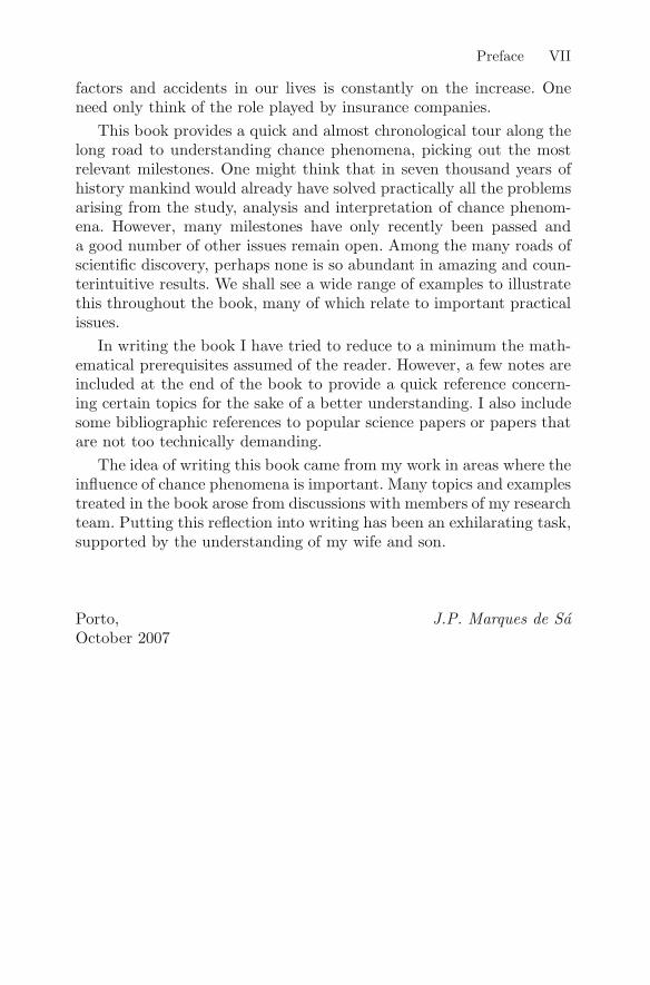
Let us now take an event such as ‘face 5 turns up’ when throwinga die. As we increase n, we verify that the frequency f tends to wanderwith decreasing amplitude around a certain value. Figure 1.4a showshow the frequencies of face 5 and face 6 might evolve with n in twodistinct series of 2 000 throws of a fair die. Some wanderings are clearlyvisible, each time with smaller amplitude as n increases, reaching a rea-sonable level of stability near the theoretical value of 1/6. Figure 1.4bshows the evolution of the frequency for a new series of 2 000 throws,now relative to faces 5 or 6 turning up. Note how the stabilizationtakes place near the theoretical value of 1/3. Frequency does thereforeexhibit the additivity required for a probability measure, for sufficientlylarge n.
1.5 The Frequency Notion of Probability 13
Fig. 1.4. Possible frequency curves in die throwing. (a) Face 5 and face 6.(b) Face 5 or 6
Let us assume that for a sufficiently high value of n, say 2 000 throws,we obtain f = 0.16 for face 5. We then assign this value to the probabil-ity of face 5 turning up. This is the value that we evaluate empirically(or estimate) for P (face 5) based on the 2 000 throws. Computing theprobabilities for the other faces in the same way, let us assume that weobtain:
P (face 1) = 0.17 , P (face 2) = 0.175 ,
P (face 3) = 0.17 , P (face 4) = 0.165 ,
P (face 5) = 0.16 , P (face 6) = 0.16 .
The elementary events are no longer equiprobable. The die is not fair(biased die) and has the tendency to turn up low values more frequentlythan high values. We also note that, since n is the sum of the differentvalues of k respecting the frequencies of all the faces, the sum of theempirical probabilities is 1.
Figure 1.5 shows the probability function of this biased die. Usingthis function we can apply the same basic rules as before. For example,
P (face higher than 4) = P (5) + P (6) = 0.16 + 0.16 = 0.32 ,
P
(face lower thanor equal to 4
)
= 1 − P
(face higher
than 4
)
= 1 − 0.32 = 0.68 ,
P (even face) = P (2) + P (4) + P (6) = 0.175 + 0.165 + 0.16 = 0.5 ,
P
(even face and lowerthan or equal to 4
)
= 0.5 × 0.68 = 0.34 .

14 1 Probabilities and Games of Chance
Fig. 1.5. Probability function of a bi-ased die
In the child birth problem, frequencies of occurrence of the two sexes ob-tained from sufficiently large birth statistics can also be used as a prob-ability measure. Assuming that the probability of boys and girls bornin Portugal is estimated by the previously mentioned frequencies –P (boy) = 0.516, P (girl) = 0.484 – then, for the problem of familieswith two children presented before, we have for Portuguese families
P (at least one boy) = P (MM) + P (MF ) + P (FM)
= 0.516 × 0.516 + 0.516 × 0.484 + 0.484 × 0.516
= 0.766 .
Some questions concerning the frequency interpretation of probabilitieswill be dealt with later. For instance, when do we consider n sufficientlylarge? For the time being, it is certainly gratifying to know that we canestimate degrees of certainty of many random phenomena. We make anexception for those phenomena that do not refer to constant conditions(e.g., the probability that Chelsea beats Manchester United) or thosethat are of a subjective nature (e.g., the probability that I will feelhappy tomorrow).
1.6 Counting Techniques
Up to now we have computed probabilities for relatively simple eventsand experiments. We now proceed to a more complicated problem:computing the probability of winning the first prize of the footballpools known as toto in many European countries. A toto entry consistsof a list of 13 football matches for the coming week. Pool entrants haveto select the result of each match, whether it will be a home win, anaway win, or neither of these, typically by marking a cross over eachof the three possibilities. In this case there is a single favorable event(the right template of crosses) in an event set that we can imagine

1.6 Counting Techniques 15
to have quite a large number of possible events (templates). But howlarge is this set? To be able to answer such questions we need to knowsome counting techniques. Abraham de Moivre was the first to presenta consistent description of such techniques in his book mentioned above.Let us consider how this works for toto. Each template can be seen asa list (or sequence) of 13 symbols, and each symbol can have one ofthree values: home win, home loss (away win) and draw, that we willdenote, respectively, by W (win), L (loss), and D (draw). A possibletemplate is thus
WWLDDDWDDDLLW .
How many such templates are there? First, assume that the toto hasonly one match. One would then have only three distinct templates,i.e., as many as there are symbols. Now let us increase the toto to twomatches. Then, for each of the symbols of the first match, there arethree different templates corresponding to the symbols of the secondmatch. There are therefore 3 × 3 = 9 templates. Adding one morematch to the toto, the next three symbols can be used with any ofthe previous templates, whence we obtain 3 × 3 × 3 templates. Thisline of thought can be repeated until one reaches the 13 toto matches,which then correspond to 313 = 1594 323 templates. This is a ratherlarge number. The probability of winning the toto by chance alone is1/1 594 323 = 0.000 000 627. In general, the number of lists of n symbolsfrom a set of k symbols is given by nk.
We now consider the problem of randomly inserting 5 different let-ters into 5 envelopes. Each envelope is assumed to correspond to oneand only one of the letters. What is the probability that all envelopesreceive the right letter? Let us name the letters by numbers 1, 2, 3, 4,5, and let us imagine that the envelopes are placed in a row, with novisible clues (sender and addressee), as shown in Fig. 1.6.
Figure 1.6 shows one possible letter sequence, namely, 12345. An-other is 12354. Only one of the possible sequences is the right one. Thequestion is: how many distinct sequences are there? Take the leftmostposition. There are 5 distinct possibilities for the first letter. Considerone of them, say 3. Now, for the four rightmost positions, letter 3 isno longer available. (Note the difference in relation to the toto case:
Fig. 1.6. Letters and envelopes

16 1 Probabilities and Games of Chance
Table 1.1. Probability P of matching n letters
n 1 2 3 4 5 10 15
P 1 0.5 0.17 0.042 0.0083 0.000 000 28 0.000000 000 000 78
the fact that a certain symbol was chosen as the first element of thelist did not imply, as here, that it could not be used again in other listpositions.) Let us then choose one of the four remaining letters for thesecond position, say, 5. Only three letters now remain for the last threepositions. So for the first position we had 5 alternatives, and for thesecond position we had 4. This line of thought is easily extended untilwe reach a total number of alternatives given by
5 × 4 × 3 × 2 × 1 = 120 .
Each of the possible alternatives is called a permutation of the 5 sym-bols. Here are all the permutations of three symbols:
123 132 213 231 312 321 .
We have 3 × 2 × 1 = 6 permutations. Note how the total numberof permutations grows dramatically when one increases from 3 to 5symbols. Whereas with 3 letters the probability of a correct match isaround 17%, for 5 letters it is only 8 in one thousand.
In general, the number of ordered sequences (permutations) of nsymbols is given by
n × (n − 1) × (n − 2) × . . . × 1 .
This function of n is called the factorial function and written n! (read nfactorial). Table 1.1 shows the fast decrease of probability P of match-ing n letters, in correspondence with the fast increase of n!. For exam-ple, for n = 10 there are 10! = 3 628 800 different permutations of theletters. If we tried to match the envelopes, aligning each permutationat a constant rate of one per second, we should have to wait 42 daysin the worst case (trying all 10! permutations). For 5 letters, 2 minuteswould be enough, but for 15 letters, 41 466 years would be needed!
Finally, let us consider tossing a coin 5 times in a row. The questionnow is: what is the probability of heads turning up 3 times? Denoteheads and tails by 1 and 0, respectively. Assume that for each heads–tails configuration we take note of the position in which heads occurs,as in the following examples:

1.6 Counting Techniques 17
Sequence Heads position
10011 1, 4, 5
01101 2, 3, 5
10110 1, 3, 4
Taking into account the set of all 5 possible posi-tions, 1, 2, 3, 4, 5, we thus intend to count thenumber of distinct subsets that can be formedusing only 3 of those 5 symbols. For this pur-pose, we start by assuming that the list of all120 permutations of 5 symbols is available andselect as subsets the first 3 permutation symbols,as illustrated in the diagram on the right.
3︷︸︸︷
123 45123 54132 45132 54...
...234 15234 51...
...
When we consider a certain subset, say 1, 2, 3, we are not concernedwith the order in which the symbols appear in the permutations. It is allthe same whether it is 123, 132, 231, or any other of the 3! = 6 permu-tations. On the other hand, for each sequence of the first three symbols,there are repetitions corresponding to the permutations of the remain-ing symbols; for instance, 123 is repeated twice, in correspondence withthe 2! = 2 permutations 45 and 54. In summary, the number of subsetsthat we can form using 3 of 5 symbols (without paying attention to theorder) is obtained by dividing the 120 permutations of 5 symbols bythe number of repetitions corresponding to the permutations of 3 andof 5 − 3 = 2 symbols. The conclusion is that
number of subsets of 3 out of 5 symbols =5!
3! × (5 − 3)!=
120
6 × 2= 10 .
In general, the number of distinct subsets (the order does not matter)
of k symbols out of a set of n symbols, denoted
(nk
)
, and called the
number of combinations of n, taking k at a time, is given by(
nk
)
=n!
k! × (n − k)!.
Let us go back to the problem of the coin tossed 5 times in a row, usinga fair coin with P (1) = P (0) = 1/2. The probability that heads turns upthree times is (1/2)3. Likewise, the probability that tails turns up twice

18 1 Probabilities and Games of Chance
Fig. 1.7. Probability of obtaining k heads in 5 throws of a fair coin (a) anda biased coin (b)
is (1/2)2. Therefore, the probability of a given sequence of three headsand two tails is computed as (1/2)3 × (1/2)2 = (1/2)5. Since there are(
53
)
distinct sequences on those conditions, we have (disjoint events)
P (3 heads in 5 throws) =
(53
)
×(
1
2
)5
=10
32= 0.31 .
Figure 1.7a shows the probability function for several k values. Notethat for k = 0 (no heads, i.e., the sequence 00000) and for k = 5 (allheads, i.e., the sequence 11111) the probability is far lower (0.031) thanwhen a number of heads near half of the throws turns up (2 or 3).
Let us suppose that the coin was biased, with a probability of 0.65of turning up heads (and, therefore, 0.35 of turning up tails). We have
P (3 heads in 5 throws) =
(53
)
× (0.65)3 × (0.35)2 = 0.336 .
For this case, as expected, sequences with more heads are favored whencompared with those with more tails, as shown in Fig. 1.7b. For in-stance, the sequence 00000 has probability 0.005, whereas the sequence11111 has probability 0.116.
1.7 Games of Chance
Games of the kind played in the casino – roulette, craps, several cardgames and, in more recent times, slot machines and the like – togetherwith any kind of national lottery are commonly called games of chance.

1.7 Games of Chance 19
All these games involve a chance phenomenon that is only very rarelyfavorable to the player. Maybe this is the reason why in some Europeanlanguages, for example, Portuguese and Spanish, these games are calledgames of bad luck, using for ‘bad luck’ a word that translates literallyto the English word ‘hazard’. The French also use ‘jeux de hasard’ torefer to games of chance. This word, meaning risk or danger, comesfrom the Arab az-zahar , which in its turn comes from the Persian azzar , meaning dice game.
Now that we have learned the basic rules for operating with proba-bilities, as well as some counting techniques, we will be able to under-stand the bad luck involved in games of chance in an objective manner.
1.7.1 Toto
We have already seen that the probability of a full template hit inthe football toto is 0.000 000 627. In order to determine the probabilityof other prizes corresponding to 11 or 12 correct hits one only has todetermine the number of different ways in which one can obtain the 11or 12 correct hits out of the 13. This amounts to counting subsets of 11or 12 symbols (the positions of the hits) of the 13 available positions. We
have seen that such counts are given by
(1312
)
and
(1311
)
, respectively.
Hence,
probability of 13 hits (1/3)13 = 0.000 000 627 ,
probability of 12 hits
(1312
)
× (1/3)13 = 0.000 008 15 ,
probability of 11 hits
(1311
)
× (1/3)13 = 0.000 048 92 .
In this example and the following, the reader must take into account thefact that the computed probabilities correspond to idealized models ofreality. For instance, in the case of toto, we are assuming that the choiceof template is made entirely at random with all 1 594 323 templatesbeing equally likely. This is not usually entirely true.
As a comparison the probability of a first toto prize is about twiceas big as the probability of a correct random insertion of 10 letters intheir respective envelopes.

20 1 Probabilities and Games of Chance
1.7.2 Lotto
The lotto or lottery is a popular form of gambling that often corre-sponds to betting on a subset of numbers. Let us consider the lottothat runs in several European countries consisting of betting on a sub-set of six numbers out of 49 (from 1 through 49). We already know howto compute the number of distinct subsets of 6 out of 49 numbers:
(496
)
=49!
6! × 43!=
49 × 48 × . . . × 1
(6 × 5 × . . . ) × (43 × 42 × . . . )= 13 983 816 .
Therefore, the probability of winning the first prize is
P (first prize: 6 hits) =1
13 983 816= 0.000 000 071 5 ,
smaller than the probability of a first prize in the toto.
Let us now compute the probability of the third prize corresponding
to a hit in 5 numbers. There are
(65
)
= 6 different ways of selecting
five numbers out of six, and the sixth number of the bet can be anyof the remaining 43 non-winning numbers. Therefore, the probabilityof winning the third prize is 6 × 43 = 258 times greater than theprobability of winning the first prize, that is,
P (third prize: 5 hits) = 258 × 0.000 000 071 5 = 0.000 018 4 .
The second prize corresponds to five hits plus a hit on a supplementarynumber, which can be any of the remaining 43 numbers. Thus, theprobability of winning the second prize is 43 times smaller than thatof the third prize:
P (second prize: 5 hits + 1 supplementary hit) = 6 × 0.000 000 071 5
= 0.000 000 429 .
In the same way one can compute
P (fourth prize: 4 hits) =
(64
)
×(
432
)
× 0.000 000 071 5
= 15 × 903 × 0.000 000 071 5 = 0.000 969 ,
P (fifth prize: 3 hits) =
(63
)
×(
433
)
× 0.000 000 071 5
= 20 × 12 341 × 0.000 000 071 5 = 0.017 65 .

1.7 Games of Chance 21
The probability of winning the fifth prize is quite a lot higher than theprobability of winning the other prizes and nearly twice as high as theprobability of matching 5 letters to their respective envelopes.
1.7.3 Poker
Poker is played with a 52 card deck (13 cards of 4 suits). A player’shand is composed of 5 cards. The game involves a betting system thatguides the action of the players (card substitution, staying in the gameor passing, and so on) according to a certain strategy depending on thehand of cards and the behavior of the other players. It is not, therefore,a game that depends only on chance. Here, we will simply analyze thechance element, computing the probabilities of obtaining specific handswhen the cards are dealt at the beginning of the game.
First of all, note that there are(
525
)
=52!
5! × 47!= 2 598 960 different 5-card hands .
Let us now consider the hand that is the most difficult to obtain, theroyal flush, consisting of an ace, king, queen, jack and ten, all of thesame suit. Since there are four suits, the probability of randomly draw-ing a royal flush (or any previously specified 5-card sequence for thatmatter), is given by
P (royal flush) =4
2 598 960= 0.000 001 5 ,
almost six times greater than the probability of winning a second prizein the toto.
Let us now look at the probability of obtaining the hand of lowestvalue, containing a simple pair of cards of the same value. We denotethe hand by AABCD, where AA corresponds to the equal-value pair ofcards. Think, for instance, of a pair of aces that can be chosen out of the
4 aces in
(42
)
= 6 different ways. As there are 13 distinct values, the
pair of cards can be chosen in 6×13 = 78 different ways. The remainingthree cards of the hand will be drawn out of the remaining 12 values,
with each card being of any of the 4 suits. There are
(123
)
combinations

22 1 Probabilities and Games of Chance
of the values of the three cards. Since each of them can come from anyof the 4 suits, we have
(123
)
× 4 × 4 × 4 = 14 080
different possibilities. Thus,
P (pair) = 13 × 14 080
2 598 960= 0.423 .
That is, a pair is almost as probable as getting heads (or tails) whentossing a coin. Using the same counting techniques, one can work outthe list of probabilities for all interesting poker hands as follows:
Pair AABCD 0.423Two pairs AABBC 0.048Three-of-a-kind AAABC 0.021Straight 5 successive values 0.0039Flush 5 cards of the same suit 0.0020Full house AAABB 0.0014Four-of-a-kind AAAAB 0.000 24Straight flush Straight + flush 0.000 015Royal flush Ace, king, queen, jack, ten
of the same suit 0.000 001 5
1.7.4 Slot Machines
The first slot machines (invented in the USA in 1897) had 3 wheels,each with 10 symbols. The wheels were set turning until they stoppedin a certain sequence of symbols. The number of possible sequences wastherefore 10×10×10 = 1000. Thus, the probability of obtaining a spe-cific winning sequence (the jackpot) was 0.001. Later on, the number ofsymbols was raised to 20, and afterwards to 22 (in 1970), corresponding,in this last case, to a 0.000 093 914 probability of winning the jackpot.The number of wheels was also increased and slot machines with re-peated symbols made their appearance. Everything was done to makeit more difficult (or even impossible!) to obtain certain prizes.
Let us look at the slot machine shown in Fig. 1.8, which as a matterof fact was actually built and came on the market with the followinglist of prizes (in dollars):

1.7 Games of Chance 23
Fig. 1.8. Wheels of a particularly infamous slot machine
Pair (of jacks or better) $ 0.05Two pairs $ 0.10Three-of-a-kind $ 0.15Straight $ 0.25Flush $ 0.30Full house $ 0.50Four-of-a-kind $ 1.00Straight flush $ 2.50Royal flush $ 5.00
The configuration of the five wheels is such that the royal flush cannever show up, although the player may have the illusion when lookingat the spinning wheels that it is actually possible. Even the straightflush only occurs for one single combination: 7, 8, 9, 10 and jack ofdiamonds. The number of possible combinations is 155 = 759 375. The

24 1 Probabilities and Games of Chance
number of favorable combinations for each winning sequence and therespective probabilities are computed as:
Pair (of jacks or better) 68 612 0.090 353Two pairs 36 978 0.048 695Three-of-a-kind 16 804 0.022 129Straight 2 396 0.003 155Flush 1 715 0.002 258Full house 506 0.000 666Four-of-a-kind 60 0.000 079Straight flush 1 0.000 001Royal flush 0 0
We observe that the probabilities of these ‘poker’ sequences for the pairand high-valued sequences are far lower than their true poker counter-parts.
The present slot machines use electronic circuitry with the finalposition of each wheel given by a randomly generated number. Theprobabilities of ‘bad luck’ are similar.
1.7.5 Roulette
The roulette consists of a sort of dish having on its rim 37 or 38 hemi-spherical pockets. A ball is thrown into the spinning dish and movesaround until it finally settles in one of the pockets and the dish (theroulette) stops. The construction and the way of operating the rouletteare presumed to be such that each throw can be considered as a ran-dom phenomenon with equiprobable outcomes for all pockets. Theseare numbered from 0. In European roulette, the numbering goes from0 to 36. American roulette has an extra pocket marked 00.
In the simplest bet the player wins if the bet is on the number thatturns up by spinning the roulette, with the exception of 0 or 00 whichare numbers reserved for the house. Thus, in European roulette theprobability of hitting a certain number is 1/37 = 0.027 (better thangetting three-of-a-kind at poker), which does not look so bad, especiallywhen one realises that the player can place bets on several numbers (aswell as on even or odd numbers, numbers marked red or black, andso on). However, we shall see later that even in ‘games of bad luck’whose elementary probabilities are not that ‘bad’, prizes and fees arearranged in such a way that in a long sequence of bets the player willlose, while maintaining the illusion that good luck really does lie justaround the corner!
2
Amazing Conditions
2.1 Conditional Events
The results obtained in the last chapter, using the basic rules for op-erating with probabilities, were in perfect agreement with commonsense. From the present chapter onwards, many surprising results willemerge, starting with the inclusion of such a humble ingredient as theassignment of conditions to events. Consider once again throwing a dieand the events ‘face less than or equal to 4’ and ‘even face’. In thelast chapter we computed P (face less than or equal to 4) = 2/3 andP (even face) = 1/2. One might ask: what is the probability that aneven face turns up if we know that a face less than or equal to 4 hasturned up? Previously, when referring to the even-face event, there wasno prior condition, or information conditioning that event. Now, thereis one condition: we know that ‘face less than or equal to 4’ has turnedup. Thus, out of the four possible elementary events corresponding to‘face less than or equal to 4’, we enumerate those that are even. Thereare two: face 2 and face 4. Therefore,
P (even face if face less than or equal to 4) =2
4=
1
2.
Looking at Fig. 1.2c of the last chapter, we see that the desired prob-ability is computed by dividing the cases corresponding to the eventintersection (hatched gray squares) by the cases corresponding to thecondition (gray squares). Briefly, from the point of view of the classicdefinition, it is as though we have moved to a new set of elementaryevents corresponding to compliance with the conditioning event, viz.,1, 2, 3, 4.

26 2 Amazing Conditions
At the same time notice that, for this example the condition did notinfluence the probability of ‘even face’:
P (even face if face less than or equal to 4) = P (even face) .
This equality does not always hold. For instance, it is an easy task tocheck that
P (even face if face less than or equal to 5) =2
5= P (even face) .
From the frequentist point of view, and denoting the events of therandom experiment simply by A and B, we may write
P (A if B) ≈ kA and B
kB,
where kA and B and kB are, respectively, the number of occurrences of‘A and B’ and ‘B’ when the random experiment is repeated n timeswith n sufficiently large. The symbol ≈ means ‘approximately equalto’. It is a well known fact that one may divide both terms of a fractionby the same number without changing its value. Therefore, we rewrite
P (A if B) ≈ kA and B
kB=
kA and B/n
kB/n,
justifying, from the frequentist point of view, the so-called conditionalprobability formula:
P (A if B) =P (A and B)
P (B).
For the above example where the random experiment consists of throw-ing a die, the formula corresponds to dividing 2/6 by 4/6, whence theabove result of 1/2. Suppose we throw a die a large number of times,say 10 000 times. In this case, about two thirds of the times we expect‘face less than or equal to 4’ to turn up. Imagine that it turned up 6 505times. From this number of times, let us say that ‘even face’ turned up3 260 times. Then the frequency of ‘even face if face less than or equalto 4’ would be computed as 3 260/6 505, close to 1/2. In other trialsthe numbers of occurrences may be different, but the final result, forsufficiently large n, will always be close to 1/2.
We now look at the problem of determining the probability of ‘faceless than or equal to 4 if even face’. Applying the above formula we get

2.2 Experimental Conditioning 27
P
(face less than or equal
to 4 if even face
)
=
P
(face less than or equal
to 4 and even face
)
P (even face)
=2/6
3/6=
2
3.
Thus, changing the order of the conditioning event will in general pro-duce different probabilities. Note, however, that the intersection is (al-ways) commutative: P (A and B) = P (B and A). In our example:
P (A and B) = P (A if B)P (B) =1
2× 2
3=
1
3,
P (B and A) = P (B if A)P (A) =2
3× 1
2=
1
3.
From now on we shall simplify notation by omitting the multiplicationsymbol when no possibility of confusion arises.
2.2 Experimental Conditioning
The literature on probability theory is full of examples in which ballsare randomly extracted from urns. Consider an urn containing 3 whiteballs, 2 red balls and 1 black ball. The probabilities of randomly ex-tracting one specific-color ball are
P (white) = 1/2 , P (red) = 1/3 , P (black) = 1/6 .
If, whenever we extract a ball, we put it back in the urn – extractionwith replacement – these probabilities will remain unchanged in the fol-lowing extractions. If, on the other hand, we do not put the ball backin the urn – extraction without replacement – the experimental con-ditions for ball extraction are changed and we obtain new probabilityvalues. For instance:
• If a white ball comes out in the first extraction, then in the followingextraction
P (white) = 2/5 , P (red) = 2/5 , P (black) = 1/5 .
• If a red ball comes out in the first extraction, then in the followingextraction:
P (white) = 3/5 , P (red) = 1/5 , P (black) = 1/5 .

28 2 Amazing Conditions
• If a black ball comes out in the first extraction, then in the followingextraction:
P (white) = 3/5 , P (red) = 2/5 , P (black) = 0 .
As we can see, the conditions under which a random experiment takesplace may drastically change the probabilities of the various eventsinvolved, as a consequence of event conditioning.
2.3 Independent Events
Let us now consider throwing two dice, one white and the other green,and suppose someone asks the following question: what is the proba-bility that an even face turns up on the white die if an even face turnsup on the green die? Obviously, if the dice-throwing is fair, the facethat turns up on the green die has no influence whatsoever on the facethat turns up on the white die, and vice versa. The events ‘even faceon the white die’ and ‘even face on the green die’ do not interfere. Thesame can be said about any other pair of events, one of which refers tothe white die while the other refers to the green die. We say that theevents are independent . Applying the preceding rule, we may work thisout in detail as
P
(even face of white die ifeven face of green die
)
=
P
(even face of white die and
even face of green die
)
P (even face of green die)
=(1/2) × (1/2)
1/2=
1
2,
which is precisely the probability of ‘even face of the white die’. Inconclusion, the condition ‘even face of the green die’ has no influenceon the probability value for the other die. Consider now the question:what is the probability of an even face of the white die turning up ifat least one even face turns up (on either of the dice or on both)? Wefirst notice that ‘at least one even face turns up’ is the complement of‘no even face turns up’, or in other words, both faces are odd, whichmay occur 3 × 3 = 9 times. Therefore,
P
(even face of the white dieif at least one even face
)
=
P
(even face of the white dieand at least one even face
)
P (at least one even face)
=3 × 6/36
(36 − 9)/36=
2
3.

2.4 A Very Special Reverend 29
We now come to the conclusion that the events ‘even face of the whitedie’ and ‘at least one even face’ are not independent. Consequently,they are said to be dependent . In the previous example of ball extractionfrom an urn, the successive extractions are independent if performedwith replacement and dependent if performed without replacement.
For independent events, P (A if B) = P (A) and P (B if A) = P (B).Let us go back to the conditional probability formula:
P (A if B) =P (A and B)
P (B), or P (A and B) = P (A if B)P (B) .
If the events are independent one may replace P (A if B) by P (A)and obtain P (A and B) = P (A)P (B). Thus, the probability formulapresented in Chap. 1 for event intersection is only applicable when theevents are independent. In general, if A,B, . . . , Z are independent,
P (A and B and . . . and Z) = P (A) × P (B) × . . . × P (Z) .
2.4 A Very Special Reverend
Sometimes an event can be obtained in distinct ways. For instance, inthe die-throwing experiment let us stipulate that event A means ‘faceless than or equal to 5’. This event may occur when either the eventB = ‘even face’ or its complement B = ‘odd face’ have occurred. Wereadily compute
P (A and B) = 2/6 , P (A and B) = 3/6 .
But the union of disjoint events ‘A and B’ and ‘A and B’ is obviouslyjust A. Applying the addition rule for disjoint events we obtain, withoutmuch surprise,
P (face less than or equal to 5) = P (A and B) + P (A and B)
=2
6+
3
6=
5
6.
In certain circumstances, we have to evaluate probabilities of inter-sections, P (A and B) and P (A and B), on the basis of conditionalprobabilities. Consider two urns, named X and Y , containing whiteand black balls. Imagine that X has 4 white and 5 black balls and Yhas 3 white and 6 black balls. One of the urns is randomly chosen and

30 2 Amazing Conditions
afterwards a ball is randomly drawn out of that urn. What is the prob-ability that a white ball is drawn? Using the preceding line of thought,we compute:
P (white ball) = P (white ball and urn X) + P (white ball and urn Y )
= P (white ball if urn X) × P (urn X)
+P (white ball if urn Y ) × P (urn Y )
=4
9× 1
2+
3
9× 1
2=
7
18= 0.39 .
In the book entitled The Doctrine of Chances by Abraham de Moivre,mentioned in the last chapter, reference was made to the urn inverseproblem, that is: What is the probability that the ball came from urnX if it turned out to be white? The solution to the inverse problem wasfirst discussed in a short document written by the Reverend ThomasBayes (1702–1761), an English priest interested in philosophical andmathematical problems. In Bayes’ work, entitled Essay Towards Solv-ing a Problem in the Doctrine of Chances, and published posthumouslyin 1763, there appears the famous Bayes’ theorem that would so sig-nificantly influence the future development of probability theory. Letus see what Bayes’ theorem tells us in the context of the urn problem.We have seen that
P (white ball) = P (white ball if urn X) × P (urn X)
+P (white ball if urn Y ) × P (urn Y ) .
Now Bayes’ theorem allows us to write
P (urn X if white ball) =P (urn X) × P (white ball if urn X)
P (white ball).
Note how the inverse conditioning probability P (urn X if white ball)depends on the direct conditioning probability P (white ball if urn X).In fact, it corresponds simply to dividing the ‘urn X’ term of itsdecomposition, expressed in the formula that we knew already, byP (white ball). Applying the concrete values of the example, we obtain
P (urn X if white ball) =(4/9) × (1/2)
7/18=
4
7.
In the same way,
P (urn Y if white ball) =(3/9) × (1/2)
7/18=
3
7.

2.4 A Very Special Reverend 31
Of course, the two probabilities add up to 1, as they should (the ballcomes either from urn X or from urn Y ). But care should be takenhere: the two conditional probabilities for the white ball do not haveto add up to 1. In fact, in this example, we have
P (white ball if urn X) + P (white ball if urn Y ) =7
9.
In the event ‘urn X if white ball’, we may consider that the drawingout of the white ball is the effect corresponding to the ‘urn X’ cause.Bayes’ theorem is often referred to as a theorem about the probabilitiesof causes (once the effects are known), and written as follows:
P (cause if effect) =P (cause) × P (effect if cause)
P (effect).
Let us examine a practical example. Consider the detection of breastcancer by means of a mammography. The mammogram (like manyother clinical analyses) is not infallible. In reality, long studies haveshown that (frequentist estimates)
P
(positive mammogram
if breast cancer
)
= 0.9 , P
(positive mammogram
if no breast cancer
)
= 0.1 .
Let us assume the random selection of a woman in a given populationof a country where it is known that (again frequentist estimates)
P (breast cancer) = 0.01 .
Using Bayes’ theorem we then compute:
P
(breast cancer if
positive mammogram
)
=0.01 × 0.9
0.01 × 0.9 + 0.99 × 0.1= 0.08 .
It is a probability that we can consider low in terms of clinical diagnos-tic, raising reasonable doubt about the isolated use of the mammogram(as for many other clinical analyses for that matter). Let us now assumethat the mammogram is prescribed following a medical consultation.The situation is then quite different: the candidate is no longer a ran-domly selected woman from the population of a country, but a womanfrom the female population that seeks a specific medical consultation(undoubtedly because she has found that something is not as it shouldbe). Now the probability of the cause (the so-called prevalence) is dif-ferent. Suppose we have determined (frequentist estimate)

32 2 Amazing Conditions
P
(breast cancer (in women
seeking specific consultation)
)
= 0.1 .
Using Bayes’ theorem, we now obtain
P
(breast cancer if
positive mammogram
)
=0.1 × 0.9
0.1 × 0.9 + 0.9 × 0.1= 0.5 .
Observe how the prevalence of the cause has dramatic consequenceswhen we infer the probability of the cause assuming that a certaineffect is verified.
Let us look at another example, namely the use of DNA tests inassessing the innocence or guilt of someone accused of a crime. Imaginethat the DNA of the suspect matches the DNA found at the crime scene,and furthermore that the probability of this happening by pure chanceis extremely low, say, one in a million, whence
P (DNA match if innocent) = 0.000 001 .
But,
P (DNA match if guilty) = 1 ,
another situation where the sum of the conditional probabilities is not1. Suppose that in principle there is no evidence favoring either theinnocence or the guilt (no one is innocent or guilty until there is proof),that is, P (innocent) = P (guilty) = 0.5. Then,
P (innocent if DNA match) =0.000 001 × 0.5
0.000 001 × 0.5 + 1 × 0.5≈ 0.000 001 .
In this case the DNA evidence is decisive. In another scenario let ussuppose that, given the circumstances of the crime and the suspect,there are good reasons for presuming innocence. Let us say that, forthe suspect to be guilty, one would require a whole set of circumstancesthat we estimate to occur only once in a hundred thousand times, thatis, in principle, P (innocent) = 0.999 99. Then,
P (innocent if DNA match) =0.000 001 × 0.999 99
0.000 001 × 0.999 99 + 1 × 0.000 01
≈ 0.09 .
In this case, in spite of the DNA evidence, the presumption of innocenceis still considerable (about one case in eleven).

2.5 Probabilities in Daily Life 33
Fig. 2.1. The risks of entering the PD if C clinic
2.5 Probabilities in Daily Life
The normal citizen often has an inaccurate perception of probabilitiesin everyday life. In fact, several studies have shown that the probabilitynotion is one of the hardest to grasp. For instance, if after flipping a cointhat turned up heads, we ask a child what will happen in the followingflip, the most probable answer is that the child will opt for tails. Theadult will have no difficulty in giving the correct answer to this simplequestion (that is, either heads or tails will turn up, meaning that bothevents are equally likely), but if the question gets more complicated anadult will easily fall into the so-called gambler’s fallacy. An example ofthis is imagining that one should place a high bet on a certain roulettenumber that has not come up for a long time.
Let us illustrate the fallacy with the situation where a coin hasbeen flipped several times and tails has been turning up each time.Most gamblers (and not only gamblers) then tend to consider that theprobability of heads turning up in the following flips will be higherthan before. The same applies to other games. Who has never saidsomething like: 30 is bound to come now; it’s time for black to showup; the 6 is hot; the odds are now on my side, and so on? It looks asif one would deem the information from previous outcomes as usefulin determining the following outcome; in other words, it is as if therewere some kind of memory in a sequence of trials. In fact, rigorously

34 2 Amazing Conditions
conducted experiments have even shown that the normal citizen hasthe tendency to believe that there is a sort of ‘memory’ phenomenonin chance devices. In this spirit, if a coin has been showing tails, whynot let it ‘rest’ for a while before playing again? Or change the coin?Suppose a coin has produced tails 30 times in a row. We will find itstrange and cast some doubts about the coin or the fairness of theplayer. On the other hand, if instead of being consecutive, the throwsare spaced over one month (say, one throw per day), maybe we wouldnot find the event so strange after all, and maybe we would not attributethe ‘cause’ of the event to the coin’s ‘memory’, but instead conjecturethat we are having an ‘unlucky month’.
Consider a raffle with 1 000 tickets and 1 000 players, but only oneprize. Once all the tickets have been sold – one ticket for each of the1 000 players – it comes out that John Doe has won the prize. In a newrepetition of the raffle John Doe wins again. It looks as if ‘luck’ is withJohn Doe. Since the two raffles are independent, the probability ofJohn Doe winning twice consecutively is (1/1000)2 = 0.000 001. This isexactly the same probability that corresponds to John Doe winning thefirst time and Richard Roe the second time. Note that this is the sameprobability as if John Doe had instead won a raffle in which a milliontickets had been sold, which would certainly seem less strange than thedouble victory in the two 1000-ticket raffles.
Let us slightly modify our problem, considering an only-one-prizeraffle with 10 000 tickets and the participation of 1 000 players, eachone buying the same number of tickets. The probability that a givenplayer (say, John Doe) wins is 0.001 (the thousand players are equallylikely to win). Meanwhile, the probability that someone wins the raffleis obviously 1 (someone has to win). Now suppose the raffle is repeatedthree times. The probability that the same player (John Doe) wins all3 times is (independent events) (0.001)3 = 0.000 000 001. However, theprobability that someone (whoever he or she may be) wins the rafflethree times is not 1, but at most 1000 × (0.001)3 = 0.000 001. In fact,any combination of three winning players has a probability (0.001)3;if the same 1 000 players play the three raffles, there are 1 000 distinctpossibilities of someone winning the three raffles, resulting in the aboveprobability. If the players are not always the same, the probabilitywill be smaller. Thus, what will amaze the common citizen is not somuch that John Doe has a probability of one in a thousand million ofwinning, but the fact that the probability of someone winning in threerepetitions is one in a million.

2.5 Probabilities in Daily Life 35
Let us now take a look at the following questions that appeared intests assessing people’s ability to understand probabilities:
1. A hat contains 10 red and 10 blue smarties. I pull out 10 and 8 arered. Which am I more likely to get next?
2. A box contains green and yellow buttons in unknown proportions.I take out 10 and 8 are yellow. Which am I more likely to get next?
3. In the last four matches between Mytholmroyd Athletics and Gig-gleswick United, Mytholmroyd have kicked off first every time, onthe toss of a coin. Which team is more likely to kick off next time?
People frequently find it difficult to give the correct answer1 to suchquestions. When dealing with conditional events and the applicationof Bayes’ theorem, the difficulty in arriving at the right answer is evengreater. Let us start with an apparently easy problem. We randomlydraw a card out of a hat containing three cards: one with both facesred, another with both faces blue, and the remaining one with one facered and the other blue. We pull a card out at random and observe thatthe face showing is red. The question is: what is the probability thatthe other face will also be red? In general, the answer one obtains isbased on the following line of thought: if the face shown is red, it canonly be one of two cards, red–red or red–blue; therefore, the probabilitythat it is red–red is 1/2. This result is wrong and the mistake in theline of thought has to do with the fact that the set of elementary eventshas been incorrectly enumerated. Let us denote the faces by R (red)and B (blue) and let us put a mark, say an asterisk , to indicate theface showing. The set of elementary events is then:
R∗R,RR∗, R∗B,RB∗, B∗B,BB∗ .
In this enumeration, R∗B means that for the red–blue card the R faceis showing, and likewise for the other cards. As for the RR card, anyof the faces can be turned up: R∗R or RR∗. In this way,
P (RR if R∗) =P (RR and R∗)
P (R∗)=
2
3.
In truth, for the three events containing R∗, namely R∗R, RR∗ andR∗B, only two correspond to the RR card.
The following problem was presented by two American psycholo-gists. A taxi was involved in a hit-and-run accident during the night.
1 Correct answers are: blue, yellow, either.

36 2 Amazing Conditions
Two taxi firms operate in the city: green and blue. The following factsare known:
• 85% of the taxis are green and 15% are blue.
• One witness identified the taxi as blue. The court tested the witness’reliability in the same conditions as on the night of the accident andconcluded that the witness correctly identified the colors 80% of thetime and failed in the other 20%.
What is the probability that the hit-and-run taxi was blue?
The psychologists found that the typical answer was 80%. Let ussee what the correct answer is. We begin by noting that
P
(witness is rightif taxi is blue
)
= 0.8 , P
(witness is wrong
if taxi is blue
)
= 0.2 .
Hence, applying Bayes’ theorem:
P
(taxi is blue
if witness is right
)
=0.15 × 0.8
0.15 × 08 + 0.85 × 0.2
= 0.41 .
We see that the desired probability is below 50% and nearly half of thetypical answer. In this and similar problems the normal citizen tendsto neglect the role of prevalences. Now the fact that blue taxis are lessprevalent than green taxis leads to a drastic decrease in the probabilityof the witness being right.
2.6 Challenging the Intuition
There are problems on probabilities that lead to apparently counter-intuitive results and are even a source of embarrassment for expertsand renowned mathematicians.
2.6.1 The Problem of the Sons
Let us go back to the problem presented in the last chapter of findingthe probability that a family with two children has at least one boy.The probability is 3/4, assuming the equiprobability of boy and girl.Let us now suppose that we have got the information that the randomlyselected family had a boy. Our question is: what is the probability that

2.6 Challenging the Intuition 37
the other child is also a boy? Using the same notation as in Chap. 1,we have
P(MM if MF,FM,MM
)=
1/4
3/4=
1
3.
This result may look strange, since apparently the fact that we knowthe sex of one child should not condition the probability relative to theother one. However, let us not forget that, as in the previous three-cardproblem, there are two distinct situations for boy–girl, namely MF andFM.
We now modify the problem involving the visit to a random familywith two children, by assuming that we knock at the door and a boyshows up. What is the probability that the other child is a boy? Itseems that nothing has changed relative to the above problem, but asa matter of fact this is not true. The event space is now
M∗M,MM∗,M∗F,F ∗M,FM∗, F ∗F,FF ∗ ,
where the asterisk denotes the child that opens the door. We are inter-ested in the conditional probability of M∗M,MM∗ if M∗M,MM∗,M∗F,FM∗ takes place. The probability is 1/2. We conclude that thesimple fact that a boy came to the door has changed the probabilities!
2.6.2 The Problem of the Aces
Consider a 5-card hand, drawn randomly from a 52-card deck, andsuppose that an ace is present in the hand. Let us further specify twocategories of hands: in one category, the ace is of clubs; in the other,the ace is any of the 4 aces. Suppose that in either category of hands weare interested in knowing the probability that at least one more ace ispresent in the hand. We are then interested in the following conditionalprobabilities:
P
(two or more aces if
an ace of clubs was drawn
)
, P
(two or more aces
if an ace was drawn
)
.
Are these probabilities equal? The intuitive answer is affirmative. Afterall an ace of clubs is an ace and it would seem to be all the same whetherit be of clubs or of something else. With a little bit more thought, wetry to assess the fact that in the second case we are dealing with anyof 4 aces, suggesting a larger number of possible combinations and,as a consequence, a larger probability. But is that really so? Let us
38 2 Amazing Conditions
actually compute the probabilities. It turns out that for this problemthe conditional probability rule is not of much help. It is preferable toresort to the classic notion and evaluate the ratio of favorable cases overpossible cases. In reality, since the evaluation of favorable cases wouldamount to counting hand configurations with two, three and four aces,it is worth trying rather to evaluate unfavorable cases, i.e., hands withonly one ace.
Let us examine the first category of hand with an ace of clubs. There
remain 51 cards and 4 positions to fill in. There are therefore
(514
)
possible cases, of which
(484
)
are unfavorable, i.e., there is no other
ace in the remaining 4 positions, whence
P
(two or more aces if
an ace of clubs was drawn
)
=
(514
)
−(
484
)
(514
) = 0.22 .
In the second category – a hand with at least one ace – the number ofpossible cases is obtained by subtracting from all possible hands thosewith no ace, which gives
possible cases
(525
)
−(
485
)
.
Concerning the unfavorable cases, once we fix an ace, we get the samenumber of unfavorable cases as before. Since there are four distinctpossibilities for fixing an ace, we have
unfavorable cases 4 ×(
484
)
.
Hence,
P
(two or more aces
if an ace was drawn
)
=
(525
)
−(
485
)
− 4 ×(
484
)
(525
)
−(
485
) = 0.12 .
We thus obtain a smaller (!) probability than in the preceding situation.This apparently strange result becomes more plausible if we inspectwhat happens in a very simple situation of two-card hands from a deck

2.6 Challenging the Intuition 39
Fig. 2.2. The problem of the aces for a very simple deck
with only 4 cards: ace and queen of hearts and clubs (see Fig. 2.2). Wesee that, when we fix the ace of clubs, the probability of a second aceis 1/3 (Fig. 2.2a). If on the other hand we are allowed any of the twoaces or both, the probability is 1/5 (Fig. 2.2b).
2.6.3 The Problem of the Birthdays
Imagine a party with a certain number of people, say n. The questionis: how large must n be so that the probability of finding two peoplewith the same birthday date (month and day) is higher than 50%?
At first sight it may seem that n will have to be quite large, perhapsas large as there are days in a year. We shall find that this is not so.The probability of a person’s birthday falling on a certain date is 1/365,ignoring leap years. Since the birthdays of the n people are independentof each other, any list of n people’s birthday dates has a probabilitygiven by the product of the n individual probabilities (refer to whatwas said before about the probability of independent events). Thus,
P((list of) n birthdays
)=
(1
365
)n
.
What is the probability that two birthdays do not coincide? Imaginethe people labeled from 1 to n. We may arbitrarily assign a value to thefirst person’s birthday, with 365 different ways of doing it. Once thisbirthday has been assigned there remain 364 possibilities for selectinga date for the second person with no coincidence; afterwards, 363 pos-sibilities are available for the third person’s birthday, and so on, up to
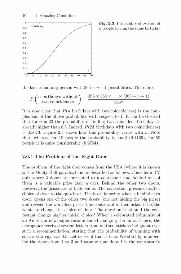
40 2 Amazing Conditions
Fig. 2.3. Probability of two out ofn people having the same birthday
the last remaining person with 365 − n + 1 possibilities. Therefore,
P
(n birthdays without
two coincidences
)
=365 × 364 × . . . × (365 − n + 1)
365n.
It is now clear that P (n birthdays with two coincidences) is the com-plement of the above probability with respect to 1. It can be checkedthat for n = 23 the probability of finding two coincident birthdays isalready higher than 0.5. Indeed, P (23 birthdays with two coincidences)= 0.5073. Figure 2.3 shows how this probability varies with n. Notethat, whereas for 10 people the probability is small (0.1169), for 50people it is quite considerable (0.9704).
2.6.4 The Problem of the Right Door
The problem of the right door comes from the USA (where it is knownas the Monty Hall paradox) and is described as follows. Consider a TVquiz where 3 doors are presented to a contestant and behind one ofthem is a valuable prize (say, a car). Behind the other two doors,however, the prizes are of little value. The contestant presents his/herchoice of door to the quiz host. The host, knowing what is behind eachdoor, opens one of the other two doors (one not hiding the big prize)and reveals the worthless prize. The contestant is then asked if he/shewants to change the choice of door. The question is: should the con-testant change his/her initial choice? When a celebrated columnist ofan American newspaper recommended changing the initial choice, thenewspaper received several letters from mathematicians indignant oversuch a recommendation, stating that the probability of winning withsuch a strategy was 0.5. Let us see if that is true. We start by number-ing the doors from 1 to 3 and assume that door 1 is the contestant’s

2.6 Challenging the Intuition 41
Table 2.1. Finding the right door
Prize door Initial choice Host opens New choice
Door 1 Door 1 Door 2 Door 3Door 2 Door 1 Door 3 Door 2
Door 3 Door 1 Door 2 Door 3
initial choice. If the contestant does not change his/her initial choice,there is a 1/3 probability of choosing the right door. If, on the otherhand, he/she decides to change his/her choice, we have the situationsshown in Table 2.1.
The contestant wins in the two new choices written in bold in thetable; therefore, the probability of winning when changing the choicedoubles to 2/3! This result is so counter-intuitive that even the Hun-garian mathematician Paul Erdos (1913–1996), famous for his contri-butions to number theory, had difficulty accepting the solution. Theproblem for most people in accepting the right solution is connectedwith the strongly intuitive and deeply rooted belief that probabilitiesare something immutable. Note, however, how the information obtainedby the host opening one of the doors changes the probability settingand allows the contestant to increase his/her probability of winning.
2.6.5 The Problem of Encounters
We saw in the last chapter that there is a 1/n! probability of randomlyinserting n letters in the right envelopes. We also noticed how thisprobability decreases very quickly with n. Let us now take a look atthe event ‘no match with any envelope’. At first sight, one could imag-ine that the probability of this event would also vary radically withn. Let us compute the probability. We begin by noticing that the one-match event has probability 1/n, whence the no-match event for oneletter has the probability 1− 1/n. If the events ‘no match for letter 1’,‘no match for letter 2’, . . . , ‘no match for letter n’ were independent,the probability we wish to compute would be (1 − 1/n)n, which tendsto 1/e, as n grows. The number denoted e, whose value up to the sixthdigit is 2.718 28, is called the Napier constant, in honor of the Scot-tish mathematician John Napier, who introduced logarithmic calculus(1618).
However, as we know, these events are not independent since theircomplements are not. For instance, if n − 1 letters are in the right

42 2 Amazing Conditions
envelope, the n th letter has only one position (the right one) to beinserted in.
It so happens that the problem we are discussing appears under sev-eral guises in practical issues, generally referred to as the problem ofencounters, which for letters and envelopes is formulated as: supposingthat the letters and the envelopes are numbered according to the natu-ral order 1, 2, . . . , n, what is the probability that, when inserting letteri, it will sit in its natural position? (We then say that an encounter hastaken place.)
Consider all the possibilities of encounters of letters 1 and 3 in a setof 5 letters:
12345 , 12354 , 14325 , 14352 , 15324 , 15342 .
We see that for r encounters (r = 2 in the example), there are only n−rletters that may permute (in the example, 3! = 6 permutations). Any ofthese permutations has probability (n−r)!/n!. Finally, we can computethe probability of no encounter as the complement of the probabilityof at least one encounter. This one is computed using a generalizationof the event union formula for more than two events. Assuming n = 3and abbreviating ‘encounter’ to ‘enc’, the probability is computed asfollows:
P
(at least one encounter
in 3 letters
)
= P (enc. letter 1) + P (enc. letter 2) + P (enc. letter 3)
− P (enc. letters 1 and 2) − P (enc. letters 1 and 3)
− P (enc. letters 2 and 3) + P (enc. letters 1, 2 and 3)
=
(31
)
× (3 − 1)!
3!−
(32
)
× (3 − 2)!
3!+
(33
)
× (3 − 3)!
3!
= 3 × 1
3− 3 × 1
6+ 1 × 1
6=
2
3.
Figure 2.4 shows the Venn diagram for this situation.
Hence,
P (no encounter in 3 letters) =1
3.
It can be shown that the above calculations can be carried out moreeasily as follows for n letters:

2.6 Challenging the Intuition 43
Fig. 2.4. The gray area in (a) is equal to the sum of the areas of the rectanglescorresponding to the events ‘enc. letter 1’, ‘enc. letter 2’, and ‘enc. letter3’, after subtracting the hatched areas in (b) and adding the double-hatchedcentral area
Table 2.2. Relevant functions for the problem of encounters
n 2 3 4 5 6 7 8 9
d(n) 1 2 9 44 265 1 854 14 833 133 496P (n) 0.5 0.333 3 0.375 0 0.366 7 0.368 1 0.367 9 0.367 9 0.367 9(1 − 1/n)n 0.25 0.296 3 0.316 4 0.327 7 0.334 9 0.339 9 0.343 6 0.346 4
P (no encounter in n letters) =d(n)
n!,
where d(n), known as the number of derangements of n elements (per-mutations without encounters) is given by
d(n) = (n − 1) ×[d(n − 1) + d(n − 2)
],
with d(0) = 1 and d(1) = 0. Table 2.2 lists the values of d(n), theprobability of no encounter in n letters denoted P (n), and the value ofthe function (1 − 1/n)n.
The probability of no encounter in n letters approaches 1/e =0.3679, as in the incorrect computation where we assumed the inde-pendence of the encounters, but it does so in a much faster way thanwith the wrong computation. Above 6 letters, the probability of nomatch in an envelope is practically constant!


3
Expecting to Win
3.1 Mathematical Expectation
We have made use in the preceding chapters of the frequentist conceptof probability. Let us assume that, in a sequence of 8 tosses of a coin,we have obtained:
heads, tails, tails, heads, heads, heads, tails, heads .
Assigning the value 1 to heads and 0 to tails, we may then add up thevalues of the sequence 10011101. We obtain 5, that is, an average valueof 5/8 = 0.625 for heads. This average, computed on the 0-1 sequence,corresponds to the frequency of occurrence f = 0.625 heads per toss.The frequentist interpretation tells us that, if we toss a coin a verylarge number of times, about half of the times heads will turn up. Inother words, on average heads will turn up once every two tosses.
As an alternative to the tossing sequence in time, we may imaginea large number of people tossing coins in the air. On average headswould turn up once for every two people. Of course this theoretical valueof 0.5 for the average (or frequency) presupposes that the coin-tossexperiment either in time or for a set of people is performed a very largenumber of times. When the number of tosses is small one expects largedeviations from an average value around 0.5. (The same phenomenonwas already illustrated in Fig. 1.4 when throwing a die.)
We now ask the reader to imagine playing a card game with someoneand using a pack with only the picture cards (king, queen, jack), theace and the joker of the usual four suits. Let us denote the cards by K,Q, J, A and F, respectively. The 4×5 = 20 cards are fairly shuffled andan attendant extracts cards one by one. After extracting and showing

46 3 Expecting to Win
Fig. 3.1. Evolution of the average gain in a card game
the card it is put back in the deck, which is then reshuffled. For eachdrawn picture card the reader wins 1 euro from the opponent and pays1 euro to the opponent if an ace is drawn and 2 euros if a joker is drawn.
Suppose the following sequence turned up:
AKAKAFJQJFAQFAAAJAAQAJAQKKFQKAJKJQJAQKKKF .
For this sequence the reader’s accumulated gain varies as: −1, 0, −1, 0,−1, −3, −2, and so on. By the end of the first five rounds the averagegain per round would be −0.2 euros (therefore, a loss). Figure 3.1 showshow the average gain varies over the above 40 rounds.
One may raise the question: what would the reader’s average gainbe in a long sequence of rounds? Each card has an equal probability ofbeing drawn, which is 4/20 = 1/5. Therefore, the 1 euro gain occursthree fifths of the time. As for the 1 or 2 euro losses, they only occurone fifth of the time. Thus, one expects the average gain in a long runto be as follows:
expected average gain = 1 × 3
5+ (−1) × 1
5+ (−2) × 1
5= 0 euro .
It thus turns out that the expected average gain (theoretical averagegain) in a long run is zero euros. In this case the game is consideredfair, that is, either the reader or the opponent has the same a priorichances of obtaining the same average gain. If, for instance, the king’svalue was 2 euros, the reader would have an a priori advantage overthe opponent, expecting to win 0.2 euros per round after many rounds.The game would be biased towards the reader. If, on the other hand,the ace’s value was −2 euros, we would have the opposite situation: thegame would be biased towards the opponent, favoring him/her by 0.2euros per round after many rounds.

3.1 Mathematical Expectation 47
Fig. 3.2. The probability function of the gain fora card game
Let us take a closer look at how the average gain is computed. Onecan look at it as if one had to deal with a variable called gain, takingvalues in the set −2,−1, 1, and such that the appropriate probabilityis assigned to each value, as shown in Fig. 3.2. One then simply addsup the products of the values with the probabilities.
We say that the gain variable is a random variable. The expectedaverage gain, expected after a large number of rounds, which, as wesaw, is computed using the event probabilities, is called the mathemat-ical expectation of the gain variable. Note the word ‘mathematical’.We may have to play an incredibly large number of times before theaverage gain per round is sufficiently near the mathematical, theoreti-cal, value of the expected average gain. At this moment the reader willprobably suspect, and rightly so, that in the coin-tossing experimentthe probability that heads turns up is the mathematical expectation ofthe random variable ‘frequency of occurrence’, denoted by f .
There is in fact a physical interpretation of the mathematical ex-pectation that we shall now explain with the help of Fig. 3.2. Imaginethat the ‘gain’ axis is a wire along which point masses have been placedwith the same value and in the same positions as in Fig. 3.2. The equi-librium point (center of gravity) of the wire would then correspond tothe mathematical expectation, in this case, the point 0.
Fig. 3.3. Evolution of the average gain in 1 000 rounds
48 3 Expecting to Win
Fig. 3.4. The euphemistic average
Figure 3.3 shows how the average gain of the card game varies overa sequence of 1 000 rounds. Note the large initial wanderings followedby a relative stabilization. Another sequence of rounds would mostcertainly lead to a different average gain sequence. However, it wouldalso stabilize close to
mathematicalexpectation
=∑
(value of random
variable
)
×(
respectiveprobability
)
,
where∑
denotes the total sum.
3.2 The Law of Large Numbers
The time has come to clarify what is meant by a ‘sufficiently long run’ or‘a large number of rounds’. For that purpose, we shall use the precedingcard game example with null mathematical expectation. Denoting theexpectation by E, we have
E(AKQJF game) = 0 .
On the other hand, the average gain after n rounds is computed byadding the individual gains of the n rounds – that is, the values of thecorresponding random variable – and dividing the resulting sum by n.In Fig. 3.1, for instance, the values of the random variable for the first10 rounds were
−1 , 1 , −1 , 1 , −1 , −2 , 1 , 1 , 1 , −2 .

3.2 The Law of Large Numbers 49
We thus obtain the following average gain in 10 rounds:
average gain in 10 rounds =−1 + 1 − 1 + 1 − 1 − 2 + 1 + 1 + 1 − 2
10= −0.2 .
Figure 3.3 shows a sequence of 1 000 rounds. This is only one sequenceout of a large number of possible sequences. With regard to the numberof possible sequences, we apply the same counting technique as for thetoto: the number of possible sequences is 51000, which is closely repre-sented by 4 followed by 71 zeros! (A number larger than the number ofatoms in the Milky Way, estimated as 1 followed by 68 zeros.)
Figure 3.5 shows 10 curves of the average gain in the AKQJF game,corresponding to 10 possible sequences of 1 000 rounds. We observea tendency for all curves to stabilize around the mathematical expec-tation 0. However, we also observe that some average gain curves thatlooked as though they were approaching zero departed from it later on.Let us suppose that we establish a certain deviation around zero, forinstance 0.08 (the broken lines in Fig. 3.5). Let us ask whether it ispossible to guarantee that, after a certain number n of rounds, all thecurves will deviate from zero by less than 0.08?
Let us see what happens in the situation shown in Fig. 3.5. Whenn = 200, we have 4 curves (out of 10) that exceed the specified de-viation. Near n = 350, we have 3 curves. After around 620, we onlyhave one curve and finally, after approximately 850, no curve exceedsthe specified deviation. This experimental evidence suggests, therefore,that the probability of finding a curve that deviates from the mathe-matical expectation by more than a pre-specified tolerance will becomesmaller and smaller as n increases.
Now, it is precisely such a law that the mathematician JacobBernoulli, already mentioned in Chap. 1, was able to demonstrate and
Fig. 3.5. Ten possible evolutions of the average gain in the card game

50 3 Expecting to Win
which has come to be known as the law of large numbers or Bernoulli’slaw : for a sequence of random variables with the same probability lawand independent from each other (in our example, no round depends onthe others), the probability that the respective average deviates fromthe mathematical expectation by more than a certain pre-establishedvalue tends to zero. Turning back to our previous question, we cannotguarantee that after a certain number of rounds all average gain curveswill deviate from the mathematical expectation by less than a certainvalue, but it is nevertheless possible to determine a degree of certainty(compute the probability) of such an event, and that degree of certaintyincreases with the number of rounds.
This way, the probability measure (for instance, of heads turning upin coin tossing) does not predict the outcome of a particular sequence,but, in a certain sense, ‘predicts’ the average outcome of a large numberof sequences. We cannot predict the detail of all possible evolutions, butwe can determine a certain global degree of certainty.
In a game between John and Mary, if John bets a million with1/1000 probability of losing and Mary bets 1000 with 999/1000 prob-ability of losing, the gain expectation is:
1 000 × 999
1 000− 1 000 000 × 1
1 000= −1 for John ,
1 000 000 × 1
1 000− 1 000 × 999
1 000= +1 for Mary .
Therefore, for sufficiently large n, the game is favorable to Mary (seeFig. 3.6). However, if the number of rounds is small, John has theadvantage.
Fig. 3.6. Evolution of John’s average gain with the number of rounds, in sixpossible sequences. Only in one sequence is chance unfavorable to John duringthe first 37 rounds

3.3 Bad Luck Games 51
When we say ‘tends to zero’, in the law of large numbers, the mean-ing is that it is possible to find a sufficiently high value of n after whichthe probability of a curve exceeding a pre-specified deviation is belowany arbitrarily low value we may wish to stipulate. We shall see laterwhat value of n that is, for this convergence in probability.
3.3 Bad Luck Games
The notion of mathematical expectation will allow us to make a betterassessment of the degree of ‘bad luck’ in so-called games of chance. Letus consider the European roulette game discussed in Chap. 1 and letus assume that a gambler only bets on a specific roulette number andfor that purpose (s)he pays 1 euro to the casino. Let us further assumethat if the gambler wins the casino will pay him/her 2 euros.
For a sufficiently large number of rounds the player’s average gainwill approach the mathematical expectation
E(roulette) = 2 × 1
37+ 0 × 36
37= 0.054 euros .
Since the player pays 1 euro for each bet, the roulette game is unfavor-able to him/her, implying an average loss of 1−0.054 = 0.946 euros perbet. The game would only be equitable if the casino paid 37 euros (!)for each winning number. On the other hand, for a two euro paymentby the casino, the game would only be equitable for the player if (s)hepaid the mathematical expectation for betting, namely 0.054 euros.
Let us now analyze the slot machine described in Chap. 1 (seeFig. 1.8). The question is: how much would a gambler have to pay forthe right to one equitable round at the slot machine? To answer thisquestion we compute the mathematical expectation using the valuespresented in Chap. 1:
E(slot machine) = 0.05 × 0.090 353 + 0.10 × 0.048 695
+0.15 × 0.022 129 + 0.25 × 0.003 155
+0.30 × 0.002 258 + 0.50 × 0.000 666
+1.00 × 0.000 079 + 2.50 × 0.000 001 = $0.01 .
Therefore the gambler should only pay 1 cent of a dollar per go.
The winning expectation in state games (lottery, lotto, toto, and thelike) is also, as can be expected, unfavorable to the gambler. Consider

52 3 Expecting to Win
the toto and let 0.35 euros be the payment for one bet. In state games,from the total amount of money amassed from the bets, only half isspent on prizes, and approximately in proportion to the probabilitiesof each type of hit. Now, as we saw in Chap. 1, for each first prize,one expects 43 second prizes, 258 third prizes, 13 545 fourth prizes and246 820 fifth prizes. Consequently, 50% of the amassed money will beused to pay prizes with a probability of:
P (prizes) = 0.000 000 071 5 × (1 + 43 + 258 + 13 545 + 246 820)
= 0.018 6 .
Therefore,
E(toto) = 0.018 6 × 0.175 − 0.9814 × 0.175 = −0.096 euros .
That is, the toto gambler loses on average (in the sense of the law oflarge numbers), 0.096 euros per bet.
3.4 The Two-Envelope Paradox
The two-envelope paradox, also known as the swap paradox, seems tohave been created by the Belgian mathematician Maurice Kraitchik(1882–1957) in 1953. There is probably no other paradox (or better,pseudo-paradox) of probability theory that has stimulated so much dis-cussion in books and papers. It is interesting to note that its enunciationis apparently simple and innocuous. Let us consider a first version ofthe paradox. Suppose I show the reader two identical and closed en-velopes with unknown contents. The only thing that is disclosed is thatthey contain certain amounts of money, with the amount in one of theenvelopes being double the amount in the other one. The reader maychoose one envelope telling me his/her choice. Having told me his/herchoice, the reader is given the possibility of swapping his/her choice.What should the reader do? Swap or not swap? It seems obvious thatany swap is superfluous. It is the same thing as if I offered the possi-bility of choosing heads or tails in the toss of a coin. The probability isalways 1/2. But let us contemplate the following line of thought:
1. The envelope I chose contains x euros.
2. The envelope I chose contains either the smaller or the biggeramount, as equally likely alternatives.

3.4 The Two-Envelope Paradox 53
3. If my envelope contains the smaller amount I will get 2x euros if Iswap and I would therefore win x euros.
4. On the other hand, if my envelope contains the bigger amount, byswapping it I will get x/2 euros and I would thus lose x/2 euros.
5. Therefore, the expected gain if I make the swap is
E(swap gain) = 0.5 × x − 0.5 × (x/2) = 0.25x euros .
That is, I should swap since the expected gain is positive. (The wisestdecision is always guided by the mathematical expectation, even if it isnot always the winning decision it is definitely the winning decision witharbitrarily high probability in a sufficiently large number of trials.) But,once the swap takes place the same argument still holds and thereforeI should keep swapping an infinite number of times!
The crux of the paradox lies in the meaning attached to x in theformula E(swap gain). Let us take a closer look by attributing a valueto x. Let us say that x is 10 euros and I am told that the amount inthe other envelope is either twice this amount (20 euros) or half of it(5 euros), with equal probability. In this case I should swap, winningon average 2.5 euros with the swap. There is no paradox in this case.Or is there? If I swap, does the same argument not hold? For supposethat the other envelope contains y euros. Therefore, the amount ofthe initially chosen envelope is either 2y euros or y/2 euros and theaverage swap gain is 0.25y euros. Then the advantage in continuingto swap ad infinitum would remain, and so would the paradox. Theproblem with this argument is that, once we have fixed x, the value ofy is not fixed: it is either 20 euros or 5 euros. Therefore we cannot usey in the computation of E(swap gain), as we did above. This aspectbecomes clear if we consider the standard version of the paradox thatwe analyze in the following.
In the standard version of the paradox what is considered fixed is thetotal amount in the two envelopes (the total amount does not depend onmy original choice). Let 3x euros be the total amount. Then, my initialchoice contains either x euros or 2x euros, and the calculation in step 5of the above argument is not legitimate, since it assumes a fixed valuefor x. If, for instance, the initial envelope contains the lower amount,x euros, I win x euros with the swap; but if it is the higher amount,2x euros, and I do not lose x/2 euros as in the formula of step 5, butin fact x euros. Therefore, E(swap gain) = 0.5x − 0.5x = 0 euros andI do not win or lose with the swap.

54 3 Expecting to Win
Other solutions to the paradox have been presented, based on thefact that the use of the formula in step 5 would lead to impossibleprobabilistic functions for the amount in one of the envelopes (see,e.g., Keith Devlin, 2005).
Do the two-envelope paradox and its analysis have any practicalinterest or is it simply an ‘entertaining problem’? In fact, this andother paradoxes do sometimes have interesting practical implications.Consider the following problem: let x be a certain amount in euros thatwe may exchange today in dollars at a rate of 1 dollar per euro, and laterconvert back to euros, at a rate of 2 dollars or 1/2 dollar per euro, withequal probability. Applying the envelope paradox reasoning we shouldperform these conversions hoping to win 0.25x euros on average. Butthen the dollar holder would make the opposite conversions and wearrive at a paradoxical situation known as the Siegel paradox , whoseconnection with the two-envelope paradox is obvious (see Friedel Bolle,2003).
3.5 The Saint Petersburg Paradox
We now discuss a coin-tossing game where a hypothetical casino (ex-tremely confident in the gambler’s fallacy) accepts to pay 2 euros ifheads turns up at the first throw, 4 euros if heads only turns up atthe second throw, 8 euros if it only turns up at the third throw, 16euros if it only turns up at the fourth throw, and so on and so forth, al-ways doubling the previous amount. The question is: how much moneyshould the player give to the casino as initial down-payment in orderto guarantee an equitable game?
The discussion and solution of this problem were first presentedby Daniel Bernoulli (nephew of Jacob Bernoulli) in his CommentariiAcademiae Scientiarum Imperialis Petropolitanae (Comments of theImperial Academy of Science of Saint Petersburg), published in 1738.The problem (of which there are several versions) came to be known asthe Saint Petersburg paradox and was the subject of abundant bibliog-raphy and discussions. Let us see why. The probability of heads turningup in the first throw is 1/2. For the second throw, taking into accountthe compound event probability rule for independent events, we have
P (first time tails) × P (second time heads) =
(1
2
)2
,

3.5 The Saint Petersburg Paradox 55
and likewise for the following throws, always multiplying the previousvalue by 1/2. In this way, as shown in Fig. 3.7b, the probability rapidlydecreases with the throw number (the random variable) when headsturns up for the first time. It then comes as no surprise that the casinoproposes to pay the player an amount that rapidly grows with the thrownumber. Applying the rule that the player must pay the mathematicalexpectation to make the game equitable, this would correspond to theplayer having to pay
E(Saint Petersburg game) = 2 × 1
2+ 4 × 1
4+ 16 × 1
16+ · · ·
= 1 + 1 + 1 + 1 + · · · = ∞ .
The player would thus have to pay an infinite (!) down-payment to thecasino in order to enter the game.
On the other hand, assuming that for entering the game the playerwould have to pay the prize value whenever no heads turned up, whenheads did finally turn up at the n th throw (s)he would have disbursed
2 + 4 + 8 + · · · + 2n−1 = 2n − 2 euros .
At the n th throw (s)he would finally get the 2n euro prize. Thus, onlya net profit of 2 euros is obtained. One is unlikely to find a gamblerwho would pay out such large amounts for such a meager profit.
The difficulty with this paradox lies in the fact that the mathe-matical expectation is infinite. Strictly, this game has no mathematicalexpectation and the law of large numbers is not applicable. The paradoxis solvable if we modify the notion of equitable game. Let us consider
Fig. 3.7. (a) The exponential growth of the gain in the paradoxical SaintPetersburg game. (b) The decreasing exponential probability in the samegame

56 3 Expecting to Win
Table 3.1. Relevant functions for the Saint Petersburg paradox
n P (n) Gain f Utility log f Expected utility[euro]
1 1/2 2 0.693 147 0.346 5742 1/4 4 1.386 294 0.693 1473 1/8 8 2.079 442 0.953 0774 1/16 16 2.772 589 1.126 3645 1/32 32 3.465 736 1.234 6686 1/64 64 4.158 883 1.299 6517 1/128 128 4.852 030 1.337 5578 1/256 256 5.545 177 1.359 2189 1/512 512 6.238 325 1.371 40310 1/1024 1024 6.931 472 1.378 172
the sum of the gains after n throws, which we denote Sn. Moreover, letus consider that, instead of a fixed amount per throw, the gambler’spayments are variable, with an accumulated payment denoted Pn aftern throws. We now modify the notion of an equitable game by imposingthe convergence in probability towards 1 of the ratio Sn/Pn. In otherwords, we would like any imbalance between what the casino and thegambler have already paid to become more and more improbable asthe number of throws increases. In this sense it is possible to guaran-tee the equitability of the Saint Petersburg game if the player pays inaccordance with the following law:
Pn = n × log2 n + 1 ,
corresponding to paying the following amounts:
1, 2, 2.76, 3.25, 3.61, 3.9, 4.14, 4.35, 4.53, 4.69, 4.83, 4.97, 5.09, 5.2, . . . .
When Daniel Bernoulli presented the Saint Petersburg paradox in 1738,he also presented a solution based on what he called the utility function.The idea is as follows. Any variation of an individual’s fortune, say f ,has different meanings depending on the value of f .
Let us denote the variation of f by ∆f . If, for instance, an individ-ual’s fortune varies by ∆f = 10000 euros, the meaning of this variationfor an individual whose fortune is f = 10000 euros (100% variation)is quite different from the meaning it has for another individual whosefortune is f = 1000 000 euros (1% variation). Let us then consider thatany transaction between individuals is deemed equivalent only whenthe values of ∆f/f are the same. This amounts to saying that there is

3.6 When the Improbable Happens 57
a utility function of the fortune f expressed by log(f). (Effectively, thebase e logarithm function – see the appendix at the end of the book– enjoys the property that its variation is expressed in that way, viz.,∆f/f .) Table 3.1 shows the expected utilities for the Saint Petersburggame, where the gain represents the fortune f . The expected utilitiesconverge to a limit (1.386 294) corresponding to 4 euros. The rationalplayer from the money-utility point of view would then pay an amountlower than 4 euros to enter the game (but we do not know whether thecasino would accept it).
3.6 When the Improbable Happens
In Chap. 1 reference was made to the problem of how to obtain headsin 5 throws, either with a fair coin – P (heads) = P (tails) = 0.5 – orwith a biased one – P (heads) = 0.65, P (tails) = 0.35. We are now ableto compute the mathematical expectation in both situations. Takinginto account the probability function for 0 through 5 heads turning upfor a fair coin (see Fig. 1.7a), we have
E(k heads in 5 throws) = 0 × 0.031 25 + 1 × 0.156 25 + 2 × 0.312 5
+3 × 0.312 5 + 4 × 0.156 25 + 5 × 0.031 25
= 2.5 .
We have obtained the entirely expected result that, for a fair coin,heads turns up on average in half of the throws (for 5-throw sequencesor any other number of throws).
There are a vast number of practical situations requiring the deter-mination of the probability of an event occurring k times in n indepen-dent repetitions of a certain random experiment. Assuming that theevent that interests us (success) has a probability p of occurring in anyof the repetitions, the probability function to use is the same as theone found in Chap. 1 for the coin example, that is,
P (k successes in n) =
(nk
)
× pk × (1 − p)n−k .
The distribution of probability values according to this formula is calledthe binomial distribution. The name comes from the fact that the prob-abilities correspond to the terms in the binomial expansion of (p + q)n,with q = 1 − p. It can be shown that the mathematical expectation ofthe binomial distribution (the distribution mean) is given by
58 3 Expecting to Win
E(binomial distribution) = n × p .
We can check this result for the above example: E = 5× 0.5 = 2.5. Forthe biased coin we have E = 5×0.65 = 3.25. Note how the expectationhas been displaced towards a higher number of heads. Note also (seeFig. 1.7) how the expectation corresponds to a central position (centerof gravity) of the probability distribution. Incidentally, from f = k/nand E(k) = np, we arrive at the result mentioned in the first section ofthis chapter that the mathematical expectation of an event frequencyis its probability, i.e., E(f) = p.
Consider a sequence of 20 throws of a fair coin in which 20 headsturned up. Looking at this sequence
1, 1, 1, 1, 1, 1, 1, 1, 1, 1, 1, 1, 1, 1, 1, 1, 1, 1, 1, 1 ,
one gets the feeling that something very peculiar has happened. As inthe gambler’s fallacy, there is a great temptation to say that, at thetwenty-first throw, the probability of turning up tails will be higher. Inother situations one might be tempted to attribute a magical or divinecause to such a sequence. The same applies to other highly organizedsequences, such as
0, 0, 0, 0, 0, 0, 0, 0, 0, 0, 1, 1, 1, 1, 1, 1, 1, 1, 1, 1 ,
or
1, 1, 0, 0, 1, 1, 0, 0, 1, 1, 0, 0, 1, 1, 0, 0, 1, 1, 0, 0 .
Nevertheless all these sequences have the same probability of occurringas any other sequence of 20 throws, namely, (1/2)20 = 0.000 000 953 67.If we repeat the 20-throw experiment a million times, we expect toobtain such sequences (or any other sequence for that matter) a numberof times given by n × p = 1000 000 × 0.000 000 95 ≈ 1. That is, thereis a high certainty that once in a million such a sequence may occur.In the case of the toto game, where the probability of the first prize is0.000 000 627, we may consider what happens if there are 1.6 millionbets. The expectation is 1, i.e., on average, we will find (with highcertainty) a first prize among 1.6 million bets. The conclusion to bedrawn is that, given a sufficiently large number of experiments, the‘improbable’ will happen: highly organized sequences, emergence of lifeon a planet, or our own existence.

3.7 Paranormal Coincidences 59
3.7 Paranormal Coincidences
Imagine yourself dreaming about the death of someone you knew. Whenreading the newspaper the next day you come across the column re-porting the death of your acquaintance. Do you have a premonitorygift? People ‘studying’ so-called paranormal phenomena often presentvarious experiences of this sort as evidence that ‘something’ such astelepathy or premonition is occurring.
Many reports on ‘weird’ cases, supposedly indicating supernaturalpowers, contain, in fact, an incorrect appreciation of the probabilitiesof coincident events. We saw in the birthday problem that it suffices tohave 23 people at a party in order to obtain a probability over 50% thattwo of them share the same birthdays. If we consider birthday datesseparated by at most one day, the number 23 can be dropped to 14!
Let us go back to the problem of dreaming about the death of some-one we knew and subsequently receiving the information that (s)he hasdied. Let us assume that in 30 years of adult life a person dreams,on average, only once about someone he/she has known during that30 year span. (This is probably a low estimate.) The probability ofdreaming about the death of an acquaintance on the day precedinghis/her death (one hit in 30× 365.25 days) is then 1/(30× 365.25). Letus further assume that in the 30 year span there are only 15 acquain-tances (friends and relatives) whose death is reported in the right timespan, so that the coincidence can be detected. With this assumption,the probability of a coincidence taking into account the 15 deaths is15/(30 × 365.25) = 1/730.5 in 30 years of one’s life. The probability ofone coincidence per year is estimated as 1/(30 × 730.5) = 0.000 045 6.Finally, let us take, for instance, the Portuguese adult population esti-mated at 7 million people. We may then use the binomial distributionformula for the mean in order to estimate how many coincidences occurper year, on average, in Portugal:
average number of coincidences per year = n × p
= 7000 000 × 0.000 045 6
= 319 .
Therefore, a ‘paranormal’ coincidence will occur, on average, aboutonce per day (and of course at a higher rate in countries with a largerpopulation). We may modify some of the previous assumptions withoutsignificantly changing the main conclusion: ‘paranormal’ coincidences

60 3 Expecting to Win
are in fact entirely normal when we consider a large population. Onceagain, given a sufficiently large number, the ‘improbable’ will happen.
3.8 The Chevalier de Mere Problem
On 29 July 1654, Pascal wrote a long letter to Fermat presenting the so-lution of a game problem raised by the Chevalier de Mere, a member ofthe court of Louis XIV already mentioned in Chap. 1. The problem wasas follows. Two players (say Primus and Secundus) bet 32 pistoles (theFrench name for a gold coin) in a heads or tails game. The 64 pistoleswould stay with the player that first obtained 3 successes (a successmight be, for instance, heads for Primus and tails for Secundus), eitherconsecutive or not. In the first round Primus wins; at that moment thetwo players are obliged to leave without ever finishing the match. Howshould the bet be divided in a fair way between them?
Fermat, in a previous letter to Pascal, had proposed a solution basedon the enumeration of all possible cases. Pascal presented Fermat withanother, more elegant solution, based on a hierarchical description ofthe problem and introducing the mathematical concept of expectation.Let us consider Pascal’s solution, based on the enumeration of all thevarious paths along which the game might have evolved. It is useful torepresent the enumeration in a tree diagram, as shown in Fig. 3.8.
The circle marked 44 corresponds to the initial situation, wherewe assume that Primus won the first round. For the moment we donot know the justification for this and other numberings of the circles.Suppose that Primus wins again; we then move to the circle marked56, following the branch marked P (Primus wins). If, on the otherhand, Secundus wins the second round, we move downwards to thecircle marked 32, in the tree branch marked S. Thus, upward branchescorrespond to Primus wins (P) and downward branches to Secunduswins (S). Note that, since a Primus loss is a Secundus win and viceversa, the match goes on for only 5 rounds. Let us now analyze the treefrom right to left (from the end to the beginning), starting with the graycircles. The circle marked 64 corresponds to a final P win, with threeheads for P according to the sequence PPSSP. P gets the 64 pistoles.The circle marked 0 corresponds to a final win for S with three tails forS according to the sequence PPSSS. Had the match been interruptedimmediately before this final round, what would P’s expectation be?We have already learned how to do this calculation:

3.8 The Chevalier de Mere Problem 61
Fig. 3.8. Tree diagram for Pascal’s solution
E(P ) = 64 × 1
2+ 0 × 1
2= 32 .
We thus obtain the situation represented by the hatched circle. For thepaths that start with PPS, we obtain in the same way, at the thirdround,
E(P ) = 64 × 1
2+ 32 × 1
2= 48 .
The process for computing the expectation repeats in the same way,progressing leftward from the end circles, until we arrive at the initialcircle to which the value 44 has been assigned. In this way, when heleaves, Primus must keep 44 pistoles and Secundus 20. A problem thatseemed difficult was easily solved using the concept of mathematicalexpectation. As a final observation, let us note that there are 10 endcircles: 10 possible sequences of rounds. Among these, Primus wins 6and Secundus 4. In spite of this, the money at stake must not be sharedin the ratio 6/10 (38.4 pistoles) for Primus and 4/10 (25.6 pistoles) forSecundus!
Once more a simple and entertaining problem has important prac-tical consequences. In fact, Pascal’s reasoning based on an end-to-startanalysis, is similar to the reasoning that leads to the price calculationof a stock market option, particularly in the context of a famous for-mula established by Fisher Black and Myron Scholes in 1973 (whichgot them the Nobel Prize for Economics in 1997).

62 3 Expecting to Win
3.9 Martingales
The quest for strategies that allow one to win games is probably asold an endeavor as mankind itself. Let us imagine the following gamebetween two opponents A and B. Both have before them a stack ofcoins, all of the same type. Each piles them up and takes out a coinfrom their stack at the same time. If the drawn coins show the sameface, A wins from B in the following way: 9 euros if it is heads–heads and1 euro if it is tails–tails. If the upper faces of the coins are different, Bwins 5 euros from A no matter whether it is heads–tails or tails–heads.Player A will tend to pile the coins up in such a way as to exhibitheads more often, expecting to find many heads–heads situations. Onthe other hand, B, knowing that A will try to show up heads, will tryto show tails.
One might think that, since the average gain in the situation thatA wins, viz., (9+1)/2, and in the situation that B wins, viz., (5+5)/2,are the same, it will not really matter how the coins are piled up.However, this is not true. First, consider A piling up the coins so thatthey always show up heads. Let t represent the fraction of the stackin which B puts heads facing up and let us see how the gain of Bvaries with t. Let us denote that gain by G. B must then pay 9 euros toA during a fraction t of the game, but will win 5 euros during a fraction1 − t of the game. That is, the gain of B is
G(stack A: heads) = −9t + 5(1 − t) = −14t + 5 .
If the coins of stack A show tails, one likewise obtains
G(stack A: tails) = +5t − 1(1 − t) = 6t − 1 .
As can be seen from Fig. 3.9, the B gain lines for the two situationsintersect at the point t = 0.3, with a positive gain for B of 0.8 euros.What has been said for a stack segment where A placed the samecoin face showing up applies to the whole stack. This means that ifB stacks his coins in such a way that three tenths of them, randomlydistributed in the stack, show up heads, he will expect to win, duringa long sequence of rounds, an average of 0.8 euros per round.
The word ‘martingale’ is used in games of chance to refer to a win-ning strategy, like the one just described. The scientific notion of mar-tingale is associated with the notion of an equitable game. This no-tion appeared for the first time in the book The Doctrine of Chanceby Abraham de Moivre, already mentioned earlier, and plays an im-portant role in probability theory and other branches of mathematics.

3.10 How Not to Lose Much in Games of Chance 63
Fig. 3.9. How the gains of B vary with a fraction t of the stack where heplays heads facing up
The word comes from the Provencal word ‘martegalo’ (originating fromthe town of Martigues), and described a leather strap that preventeda horse from lifting up its head. A martingale is similarly intended tohold sway over chance.
One must distinguish true and false martingales. Publications some-times appear proposing winning systems for the lotto, toto, and so on.One such system for winning the lotto is based on the analysis of graphsrepresenting the frequency of occurrence of each number as well as com-binations of numbers. Of course such information does not allow one toforecast the winning bet; this is just one more version of the gambler’sfallacy. Other false martingales are more subtle, like the one that weshall describe at the end of Chap. 4.
3.10 How Not to Lose Much in Games of Chance
Let us suppose that the reader, possessing an initial capital of I euros,has decided to play roulette with even–odd- or red–black-type bets, setat a constant value of a euros. The gain–loss sequence constitutes, inthis case, a coin-tossing type of sequence, with probability p = 18/37 =0.486 of winning and q = 1−p of losing. Let us further suppose that thereader decides at the outset to keep playing either until he/she winsF euros or until ruined by losing the initial capital. Jacob Bernoullidemonstrated in 1680 that such a game ends in a finite number ofsteps with a winning probability given by

64 3 Expecting to Win
Table 3.2. Roulette for different size bets. F represents the winnings at whichthe player stops and P (F ) is the probability of reaching that value
50 euro bets 100 euro bets 200 euro bets
F P (F ) F P (F ) F P (F )
1050 0.9225 1100 0.8826 1200 0.8100
1100 0.8527 1200 0.7853 1400 0.67471150 0.7896 1300 0.7034 1600 0.57361200 0.7324 1400 0.6337 1800 0.49521250 0.6804 1500 0.5736 2000 0.43281300 0.6330 1600 0.5215 2200 0.38201350 0.5896 1700 0.4758 2400 0.33991400 0.5498 1800 0.4356 2600 0.3045
P (winning F ) = P (F ) =1 − (q/p)I/a
1 − (q/p)F/a.
In the case of roulette, q/p = 1.0556. If the reader starts with aninitial capital of 1 000 euros and makes 50-euro bets, the probability ofreaching 1 200 euros is given by
P (F ) =1 − 1.055620
1 − 1.055624= 0.7324 .
Table 3.2 shows what happens when we make constant bets of 50, 100and 200 euros.
Looking at the values for situations with F = 1200 euros, printedin bold in the table, we see that the gambler would be advised to stayin the game the least time possible, whence he must risk the high-est possible amount in a single move. In the above example one sin-gle 200-euro bet has 81% probability of reaching the goal set by thegambler. This probability value is near the theoretical maximum valueP (F ) = 1000/1200 = 83.33%. If the bet amounts can vary, there arethen betting strategies to obtain a probability close to that maximumvalue. One such strategy, proposed by Lester Dubins and Leonard Sav-age in 1956, is inspired by the idea of always betting the highest possibleamount that allows one to reach the proposed goal. In the example wehave been discussing, we should then set the sequence of bets as shownin Fig. 3.10.
The following probabilities can be computed from the diagram:
P (going from 1000 to 1200) = p + q × P (going from 800 to 1200) ,

3.10 How Not to Lose Much in Games of Chance 65
Fig. 3.10. The daring bet strategy proposed by Dubins and Savage
P (going from 800 to 1200) = p + q × p × P (going from 800 to 1200) .
From this one concludes that
P (going from 1000 to 1200) = p +qp
1 − qp= 0.8195 ,
closer to the theoretical maximum.
As a final remark let us point out that the martingale of Dubinsand Savage looks quite close to a martingale proposed by the Frenchmathematician Jean Le Rond d’Alembert (1717–1783), according towhich the gambler should keep doubling his/her bet until he/she winsor until he/she has enough money to double the bet. For the aboveexample, this would correspond to stopping when reaching 400 euros,with a probability of winning of 0.7363.
Needless to say, these martingales should not be viewed as an in-citement to gambling – quite the opposite. As a matter of fact, thereis even a result about when one should stop a constant-bet game ofchance in order to maximize the winning expectation. The result is:don’t play at all! In the meantime we would like to draw the reader’sattention to the fact that all these game-derived results have plenty ofpractical applications in different areas of human knowledge.

4
The Wonderful Curve
4.1 Approximating the Binomial Law
The binomial distribution was introduced in Chap. 1 and its mathe-matical expectation in the last chapter. We saw how the binomial lawallows us to determine the probability that an event, of which we knowthe individual probability, occurs a certain number of times when thecorresponding random experiment is repeated.
Take for instance the following problem. The probability that a pa-tient gets infected with a certain bacterial strain in a given hospitalenvironment is p = 0.0055. What is the probability of finding morethan 10 infected people in such a hospital with 1000 patients? Apply-ing the binomial law, we have
P
(more than 10events in 1000
)
= P (11 events) + P (12 events)
+ · · · + P (1000 events)
=
(100011
)
× 0.005511 × 0.9945989
+
(100012
)
× 0.005511 × 0.9945988
+ · · · +(
10001000
)
× 0.00551000 × 0.99450 .
The difficulty in carrying out these calculations can be easily imagined.
For instance, calculating
(1000500
)
involves performing the multiplica-
tion 1000 × 999 × . . . × 501 and then dividing by 500 × 499 × . . . × 2.

68 4 The Wonderful Curve
Fig. 4.1. De Moivre’s approximation (open circles) of the binomial distribu-tion (black bars). (a) n = 5. (b) n = 30
Even if one applies the complement rule – subtracting from 1 the sumof the probabilities of 0 through 10 events – one still gets entangled inpainful calculations. When using a computer, it is not uncommon forthis type of calculation to exceed the number representation capacity.
Abraham de Moivre, mentioned several times in previous chapters,was the first to find the need to apply an easier way of computing fac-torials. (In his day, performing the above calculations was an extremelytedious task.) That easier way (known as Stirling’s formula) led himto an approximation of the binomial law for high values of n. Denot-ing the mathematical expectation of the binomial distribution by m(m = np) and the quantity np(1−p) by v, the approximation obtainedby Abraham de Moivre, assuming that m is not too small, was thefollowing:
(nk
)
× pk × (1 − p)n−k ≈ 1√2πv × e(k−m)2/2v
.
We have already found Napier’s number, universally denoted by theletter e, with the approximate value 2.7, when discussing the problemof encounters (Chap. 2). Let us see if De Moivre’s approximation worksfor the example in Chap. 1 of obtaining 3 heads in 5 throws of a faircoin:
m = np = 52 = 2.5 , v = np(1 − p) = 2.5
2 = 1.25 ,
k − m = 3 − 2.5 = 0.5 ,
whence
P (3 heads in 5 throws) ≈ 1√7.85 × 2.70.25/2.5
=1
2.8 × 2.70.1= 0.32 ,

4.2 Errors and the Bell Curve 69
which is really quite close to the value of 0.31 we found in Chap. 1.Figure 4.1 shows the probability function of the binomial distribution(bars) for n = 5 and n = 30 and Abraham de Moivre’s approximation(open circles). For n = 5, the maximum deviation is 0.011; for n = 30,the maximum deviation comes down to a mere 0.0012.
4.2 Errors and the Bell Curve
Abraham de Moivre’s approximation (described in a paper published in1738, with the second edition of the book The Doctrine of Chances) wasafterwards worked out in detail by the French mathematician Pierre-Simon Laplace (1749–1827) in his book Theorie Analytique des Proba-bilites (1812) and used to analyze the errors in astronomical measure-ments. More or less at the same time (1809), the German mathemati-cian Johann Carl Friedrich Gauss (1777–1855) rigorously justified thedistribution of certain sequences of measurement errors (particularlygeodesic measurements) in agreement with that formula.
It is important at this point to draw the reader’s attention to thefact that, in science, the word ‘error’ does not have its everyday mean-ing of ‘fault’ or ‘mistake’. This semantic difference is often misunder-stood. When measuring experimental outcomes, the word ‘error’ refersto the unavoidable uncertainty associated with any measurement, how-ever aptly and carefully the measurement procedure has been applied.The error (uncertainty) associated with a measurement is, therefore,the effect of chance phenomena; in other words, it is a random vari-able.
Consider weighing a necklace using the spring balance with 2 gminimum scale resolution shown in Fig. 4.2. Suppose you measure 45 gfor the weight of the necklace. There are several uncertainty factorsinfluencing this measurement:
• The measurement system resolution: the balance hand and the scalelines have a certain width. Since the hand of Fig. 4.2 has a widthalmost corresponding to 1 g, it is difficult to discriminate weightsdiffering by less than 1 g.
• The interpolation error that leads one to measure 45 g because thescale hand was approximately half-way between 44 g and 46 g.
• The parallax error , related to the fact that it is difficult to guaranteea perfect vertical alignment of our line of sight and the scale plane;for instance, in Fig. 4.2, if we look at the hand with our line of sight

70 4 The Wonderful Curve
Fig. 4.2. Spring balance with 2 g min-imum resolution
to its right, we read a value close to 250 g; if we look to its left, weread a value close to 2 g.
• The background noise, corresponding in this case to spring vibra-tions that are transmitted to the hand.
If we use a digital balance, we eliminate the parallax and interpolationerrors, but the effects of limited resolution (the electronic sensor doesnot measure pressures below a certain value) and background noise(such as the thermal noise in the electronic circuitry) are still present.
Conscious of these uncertainty factors, suppose we weighed the neck-lace fifty times and obtained the following sequence of fifty measure-ments:
44, 45, 46, 43, 47, 47, 45, 48, 48, 44, 43, 45, 46, 44, 43, 44, 45, 49, 46, 48,
45, 43, 46, 45, 44, 44, 45, 45, 46, 45, 46, 48, 47, 44, 49, 44, 47, 45, 46, 48,
46, 46, 47, 49, 45, 45, 47, 46, 46, 45 .
The average weight is 45.68 g. It seems reasonable to consider thatsince the various error sources act independently of one other, withcontributions on either side of the true value, the errors should havea tendency to cancel out when the weight is determined in a long se-ries of measurements. Things happen as though the values of a randomvariable (the ‘error’) were added to the true necklace weight, this ran-dom variable having zero mathematical expectation. In a long sequence

4.2 Errors and the Bell Curve 71
of measurements we expect, from the law of large numbers, the averageof the errors to be close to zero, and we thus obtain the true weightvalue.
Let us therefore take 45.68 g as the true necklace weight and considernow the percentage of times that a certain error value will occur (byfirst subtracting the average from each value of the above sequence).Figure 4.3 shows how these percentages (vertical bars) vary with theerror value. This graphical representation of frequencies of occurrenceof a given random variable (the error, in our case) is called a histogram.For instance, an error of 0.68 g occurred 13 times, which is 26% of thetime.
Laplace and Gauss discovered independently that, for many errorsequences of the most varied nature (relating to astronomical, geodesic,geomagnetic, electromagnetic measurements, and so on), the frequencydistributions of the errors were well approximated by the values of thefunction
f(x) =1√2πν
e−x2/2ν ,
where x is the error variable and ν represents the so-called mean squareerror. Let us try to understand this. If we subtract the average weightfrom the above measurement sequence, we obtain the following error se-quence: −1.68, −0.68, 0.32, −2.68, 1.32, 1.32, −0.68, 2.32, 2.32, −1.68,−2.68, etc. We see that there are positive and negative errors. If we getmany errors of high magnitude, no matter whether they are positive ornegative, the graph in Fig. 4.3 will become significantly stretched. Inthe opposite direction, if all the errors are of very small magnitude thewhole error distribution will be concentrated around zero. Now, oneway to focus on the contribution of each error to the larger or smaller
Fig. 4.3. Error histogramwhen weighing a necklace

72 4 The Wonderful Curve
stretching of the graph but regardless of its sign (positive or negative)consists in taking its square. So when we add the squares of all errorsand divide by their number, we obtain a measure of the spread of theerror distribution. The mean square error is precisely such a measureof the spread:
ν =1.682 + 0.682 + 0.322 + 2.682 + 1.322
50= 2.58 g2 .
The mean square error ν, is also called the variance. The square root ofthe variance, viz., s =
√ν, is called the standard deviation. In Fig. 4.3,
the value of the standard deviation (√
2.58 = 1.61 g) is indicated bythe double-ended arrow.
The dotted line in Fig. 4.3 also shows the graph of the functionf(x) found by Laplace and Gauss, and computed with ν = 2.58 g2.We see that the function seems to provide a reasonable approximationto the histogram values. As we increase the number of measurementrepetitions the function gradually fits better until values of bars arepractically indistinguishable from values taken from the dotted line.This bell-shaped curve often appears when we study chance phenom-ena. Gauss called it the normal distribution curve, because error dis-tributions normally follow such a law.
4.3 A Continuum of Chances
Let us picture a rifle shooting at a target like the one shown in Fig. 4.4.The rifle is assumed to be at a perfectly fixed position, aiming at thetarget center. Despite the fixed rifle position, the position of the bulletimpact is random, depending on chance phenomena such as the wind,rifle vibrations, barrel heating, barrel grooves wearing out, and so on.
If we use the frequentist interpretation of probability, we may easilyobtain probability estimates of hitting a certain target area. For in-stance, if out of 5000 shots hitting the target 2000 fall in the innermostcircle, an estimate of P (shot in innermost circle) is 2/5. We may applythe same procedure to the outermost circle; suppose we obtained 3/5.The estimated probability of a hit in the circular ring is then 1/5 andof a hit outside the outermost circle is 1− 3/5 = 2/5. We are assumingthat by construction there can be no shots falling outside the target.
We now proceed to consider a small circular area of the target (inany arbitrarily chosen position) for which we determine by the aboveprocedure the probability of a hit. Suppose we go on decreasing the

4.3 A Continuum of Chances 73
Fig. 4.4. Shooting at a target
circle radius, therefore shrinking the circular region. The probabilityof a hit will also decrease in a way approximately proportional to thearea of the circle when the area is sufficiently small and the shots areuniformly spread out over the circle. In other words, there comes a timewhen P (shot in the circle) is approximately given by k × a, where a isthe area of the circle and k is a proportionality factor. In order to obtainarbitrarily good estimates of P (shot in the circle) for a certain value ofa, we would of course need a large number of shots on the target, andall the more as a gets smaller.
We thus draw two conclusions from our imaginary experiment ofshooting at a target: the hit probability in a certain region continu-ally decreases as the region shrinks; for sufficiently small regions, theprobability is practically proportional to the area of the region. It is asif the total probability, 1, of hitting the target was finely smeared outover the whole target. In a very small region we can speak of probabilitydensity per unit area, and our previous k factor is
k =P (shot in region)
a.
When the region shrinks right down to a point, the probability of a hitis zero because the area is zero:
P (hit a point) = 0 (always, in continuous domains) .
We are now going to imagine that the whole rifle contraption wasmounted in such a way that the shots could only hit certain pre-established points in the target and nothing else. If we randomly selecta small region and proceed to shrink it, we will almost always obtaindiscontinuous variations of P (shot in region), depending on whetherthe region includes the pre-established points or not. In this case the

74 4 The Wonderful Curve
probability of hitting a point is not zero for the pre-established points.The total probability is not continuously smeared out on the target; itis discretely divided among the pre-established points. The domain ofpossible impact points is no longer continuous but discrete. We have infact the situation of point-like probabilities of discrete events (the pre-established points) that we have already considered in the precedingchapters.
Let us now go back to the issue of P (hit a point) equalling zerofor continuous domains. Does this mean that the point-bullet neverhits a specified point? Surely not! But it does it a finite number oftimes when the number of shots is infinite, so that, according to thefrequentist approach, the value of P (hit a point) is 0. On the otherhand, for discrete domains (shots at pre-established points), hittinga specific point would also happen an infinite number of times.
Operating with probabilities in a continuum of chances demandssome extension of the notions we have already learned (not to men-tion some technical difficulties that we will not discuss). In order todo that, let us consider a similar situation to shooting at a target, butrather simpler, with the ‘shot’ on a straight-line segment. Once againthe probability of hitting a given point is zero. However, the probabilityof the shot falling into a given straight line interval is not zero. We maydivide the interval into smaller intervals and still obtain non-zero prob-abilities. It is as if our degree of certainty that the shot falls in a giveninterval were finely smeared out along the line segment, resulting ina probability density per unit length. Thinking of the probability mea-sure as a mass, there would exist a mass density along the line segment(and along any segment interval). Figure 4.5a illustrates this situation:a line segment, between 0 and 1, has a certain probability density ofa hit. Many of the bullets shot by the rifle fall near the center (darkgray); as we move towards the segment ends, the hit probability den-sity decreases. The figure also shows the probability density function,abbreviated to p.d.f. We see how the probability density is large at thecenter and drops towards the segment ends. If we wish to determinethe probability of a shot hitting the interval from 0.6 to 0.8, we haveonly to determine the hatched area of Fig. 4.5a. (In the mass analogy,the hatched area is the mass of the interval.) In Fig. 4.5b, the probabil-ity density is constant. No interval is favored with more hits than anyother equal-length interval. This is the so-called uniform distribution.Uniformity is the equivalent for continuous domains of equiprobability(equal likelihood) for discrete domains.

4.4 Buffon’s Needle 75
Fig. 4.5. Two cases of the probability density of shots on [0, 1]. (a) Thedensity is larger at the center. (b) The density is uniform
In the initial situation of shooting at a target, the p.d.f. is a certainsurface, high at the center and decaying towards the periphery. Theprobability in a certain region corresponds to the volume enclosed bythe surface on that region. In the two situations, either the total area(Fig. 4.5) or the total volume (Fig. 4.4) represents the probability ofthe sure event, that is, they are equal to 1. Previously, in order to de-termine the probability of an event supported by a discrete domain, weadded probabilities of elementary events. Now, in continuous domains,we substitute sums by areas and volumes. With the exception of thismodification, we can continue to use the basic rules of Chap. 1.
The normal probability function presented in the last section is infact a probability density function. In the measurement error example,the respective values do not constitute a continuum; it is easy to see thatthe values are discrete (for instance, there are no error values between0.32 g and 0.68 g). Moreover, the error set is not infinite. Here as inother situations one must bear in mind that a continuous distributionis merely a mathematical model of reality.
4.4 Buffon’s Needle
Georges-Louis Leclerc, Count of Buffon (1707–1788), is known for hisremarkable contributions to zoology, botany, geology and in particularfor a range of bold ideas, many ahead of his time. For instance, heargued that natural causes formed the planets and that life on Earthwas the consequence of the formation of organic essences resulting fromthe action of heat on bituminous substances. Less well known is hisimportant contribution to mathematics, and particularly to probabilitytheory.
Buffon can be considered a pioneer in the experimental study andapplication of probability theory, a specific example of which is the fa-mous Buffon’s needle. It can be described as follows. Consider randomlythrowing a needle of length l on a floor with parallel lines separated by

76 4 The Wonderful Curve
Fig. 4.6. Area under the curve y = e−x
d ≥ l (think, for instance, of the plank separations of a wooden floor).What is the probability that the needle falls over a line?
We are dealing here with a problem of continuous probabilities sug-gested to Buffon by a fashionable game of his time known as franc-carreau. The idea was to bet that a coin tossed over a tile floor wouldfall completely inside a tile. For the needle problem, Buffon demon-strated that the required probability is given by
P =2l
πλ.
For d = l, one then obtains 2/π, i.e., Buffon’s needle experiment offersa way of computing π ! The interested reader may find several Internetsites with simulations of Buffon’s needle experiment and estimates ofπ using this method.
4.5 Monte Carlo Methods
It seems that Buffon did indeed perform long series of needle throws ona floor in order to verify experimentally the result that he had concludedmathematically. Nowadays, we hardly would engage in such labor, sincewe dispose of a superb tool for carrying out any experiments relatingto chance phenomena: the computer.
The Monte Carlo method – due to the mathematician StanislawUlam (1909–1984) – refers to any problem-solving method based onthe use of random numbers, usually with computers.
Consider the problem of computing the shaded area of Fig. 4.6 cir-cumscribed by a unit square. In this example, the formula of the curve

4.5 Monte Carlo Methods 77
delimiting the area of interest is assumed to be known, in this casey = e−x. This allows us, by mathematical operations, to obtain thevalue of the area as 1 − 1/e, and hence the value of e. However, it of-ten happens that the curve formula is such that one cannot directlydetermine the value of the area, or the formula may even be unknown.In such cases one has to resort to numerical methods. A well-knownmethod for computing area is to divide the horizontal axis into suffi-ciently small intervals and add up the vertical ‘slices’ of the relevantregion, approximating each slice by a trapezium. Such computationmethods are deterministic: they use a well defined rule.
In certain situations it may be more attractive (in particular, withregard to computation time) to use another approach that is said to bestochastic (from the Greek ‘stokhastikos’ for a phenomenon or methodwhose individual cases depend on chance) because it uses probabilities.Let us investigate the stochastic or Monte Carlo method for computingarea. For this purpose we imagine that we randomly throw points ina haphazard way onto the domain containing the interesting area (thesquare domain of Fig. 4.6). We also assume that the randomly thrownpoints are uniformly distributed in the respective domain; that is, fora sufficiently large number of points any equal area subdomain hasan equal probability of being hit by a point. Figure 4.7 shows sets ofpoints obtained with a uniform probability density function, thrownonto a unit square. Let d be the number of points falling inside therelevant region and n the total number of points thrown. Then, forsufficiently large n, the ratio d/n is an estimate of the relevant areawith given accuracy (according to the law of large numbers).
This method is easy to implement using a computer. We only needa random number generator , that is, a function that supplies num-
Fig. 4.7. Examples of uniformly distributed points. (a) 100 points. (b) 4000points

78 4 The Wonderful Curve
0 1 2 3 4 5 6 7 8 9 10
x 104
2.6
2.65
2.7
2.75
2.8
2.85
n
e(n
)Fig. 4.8. Six Monte Carlotrials for the estimation of e
bers as if they were generated by a random process. (One could alsouse roulette-generated numbers, whence the name Monte Carlo.) Manyprogramming languages provide random (in fact, pseudo-random) num-ber generating functions. The randomness of the generated numbers(the quality of the generator) has an influence on the results of MonteCarlo methods.
Figure 4.8 shows the dependence e(n) of the estimate e on n in sixMonte Carlo trials corresponding to Fig. 4.6. By inspection of Fig. 4.8,one sees that the law of large numbers is also at work here. The estimatetends to stabilize around the value of e (dotted line) for sufficientlylarge n.
Monte Carlo methods as described here are currently used in manyscientific and technical areas: aerodynamic studies, forecasts involvinga large number of variables (meteorology, economics, etc.), optimizationproblems, special effects in movies, video games, to name but a few.
4.6 Normal and Binomial Distributions
If the reader compares the formula approximating the binomial dis-tribution, found by Abraham de Moivre, and the probability densityfunction of the normal distribution, found by Laplace and Gauss, (s)hewill immediately notice their similarity. As a matter of fact, for largen, the binomial distribution is well approximated by the normal one, ifone uses
x = k − m , m = np , ν = np(1 − p) .

4.7 Distribution of the Arithmetic Mean 79
Fig. 4.9. The valueof P (more than10 events in 1000)(shaded area) usingthe normal approxi-mation
The mathematical expectation (mean) of the normal distribution isthe same as that of the binomial distribution: m = np. The variance isnp(1 − p), whence the standard deviation is s =
√
np(1 − p).
We can now go back to the initial problem of this chapter. Forn = 1000 the approximation of the normal law to the binomial law isexcellent (it is usually considered good for most applications when n islarger than 20 and the product np is not too low, conditions satisfiedin our example). Let us then consider the normal law using
m = np = 1000 × 0.0055 = 5.5 ,
ν = np(1 − p) = 5.5 × 0.9945 = 5.47 ,
whence s = 2.34.
We then have the value of P (more than 10 events in 1000) corre-sponding to the shaded area of Fig. 4.9. There are tables and computerprograms that supply values of the normal p.d.f. areas.1 In this way,one can obtain the value of the area as 0.01. The probability of find-ing more than 10 infected people among the 1000 hospital patients istherefore 1%.
4.7 Distribution of the Arithmetic Mean
When talking about the measurement error problem we mentioned thearithmetic mean as a better estimate of the desired measurement. Weare now in a position to analyze this matter in greater detail.
Consider a sequence of n values, obtained independently of eachother and originating from identical random phenomena. Such is the
1 Assuming zero mean and unit variance. Simple manipulations are required to find
the area for other values.

80 4 The Wonderful Curve
usual measurement scenario: no measurement depends on the othersand all of them are under the influence of the same random errorsources. An important result, independently discovered by Laplace andGauss, is the following: if each measurement follows the normal dis-tribution with mean (mathematical expectation) m and standard de-viation s, then, under the above conditions, the arithmetic mean (thecomputed average) random variable also follows the normal distributionwith the same mean (mathematical expectation) and with standard de-viation given by s/
√n.
Let us assume that in the necklace weighing example some divin-ity had informed us that the true necklace weight was 45 g and thetrue standard deviation of the measurement process was 1.5 g. InFig. 4.10, the solid line shows the normal p.d.f. relative to one mea-surement while the dotted line shows the p.d.f. of the arithmetic meanof 10 measurements. Both have the same mathematical expectationof 45 g. However, the standard deviation of the arithmetic mean iss/√
n = 1.5/√
10 = 0.47 g, about three times smaller; the p.d.f. of thearithmetic mean is therefore about three times more concentrated, asillustrated in Fig. 4.10. As we increase the number of measurements thedistribution of the arithmetic mean gets gradually more concentrated,forcing it to converge rapidly (in probability) to the mathematical ex-pectation. We may then interpret the mathematical expectation as the‘true value of the arithmetic mean’ (‘the true weight value for the neck-lace’) that would be obtained had we performed an infinite number ofmeasurements.
Suppose we wish to determine an interval of weights around thetrue weight value into which one measurement would fall with 95%probability. It so happens that, for a normal p.d.f., such an intervalstarts (to a good approximation) at the distribution mean minus two
Fig. 4.10. Weighing a necklace: p.d.f. of the error in a single measurement(solid curve) and for the average of 10 measurements (dotted curve)

4.7 Distribution of the Arithmetic Mean 81
standard deviations and ends at the mean plus two standard deviations.Thus, for the necklace example, the interval is 45± 3 g (3 = 2× 1.5). Ifwe take the average of 10 measurements, the interval is then 45±0.94 g(0.94 = 2 × 0.47).
In conclusion, whereas for one measurement one has a 95% degreeof certainty that it will fall in the interval 45 ± 3 g, for the averageof 10 measurements and the same degree of certainty, the interval isreduced to 45±0.94 g. Therefore, the weight estimate is clearly better:in the first case 95 out of 100 measurements will produce results thatmay be 3 g away from the true value; in the second case 95 out of100 averages of 10 measurements will produce results that are at mostabout 1 gram away. Computing averages of repeated measurements isclearly an advantageous method in order to obtain better estimates,and for this reason it is widely used in practice.
The difficulty with the above calculations is that no divinity tellsus the true values of the mean and standard deviation. (If it told us,we would not have to worry about this problem at all.) Supposing wecomputed the arithmetic mean and the standard deviation of 10 mea-surements many times, we would get a situation like the one illustratedin Fig. 4.11, which shows, for every 10-measurement set, the arithmeticmean (solid circle) plus or minus two standard deviations (double-endedsegment) computed from the respective mean square errors. The fig-ure shows 15 sets of 10 measurements, with trials numbered 1 through15. The arithmetic means and standard deviations vary for each 10-measurement set; it can be shown, however, that in a large number oftrials nearly 95% of the intervals ‘arithmetic mean plus or minus twostandard deviations’ contain the true mean value (the value that onlythe gods know). In Fig. 4.11, 14 out of the 15 segments, i.e., 93% ofthe segments, intersect the line corresponding to the true mean value.
What can then be said when computing the arithmetic mean andstandard deviation of a set of measurements? For the necklace exampleone computes for the fifty measurements:
m = 45.68 g , s = 1.61 g .
The standard deviation of the arithmetic mean is therefore 1.61/√
50 =0.23 g. The interval corresponding to two standard deviations is thus45.68±0.46 g. This interval is usually called the 95% confidence intervalof the arithmetic mean, and indeed 95% certainty is a popular valuefor confidence intervals.
What does it mean to say that the 95% confidence interval of thenecklace’s measured weight is 45.68±0.46 g? Does it mean that we are

82 4 The Wonderful Curve
Fig. 4.11. Computed mean±2 standard deviations inseveral trials (numbered 1to 15) of 10 measurements
95% sure that the true value is inside that interval? This is an oft-statedbut totally incorrect interpretation. In fact, if the true weight were 45 gand the true standard deviation were 3 g, we have already seen that,with 95% certainty, the average of the 50 measurements would fall inthe interval 45 ± 0.94 g, and not in 45.68 ± 0.46 g. Whatever the truevalues of the mean and standard deviation may be, there will alwaysexist 50-measurement sets with confidence intervals distinct from theconfidence interval of the true mean value. The interpretation is quitedifferent and much more subtle.
Figure 4.11 can help us to work out the correct interpretation. Whencomputing the 95% confidence interval, we are computing an intervalthat will not contain the true mean value only 5% of the time. We mayhave had such bad luck that the 50-measurement set obtained is likeset 8 in Fig. 4.11, a set that does not contain the true mean value.For this set there is 100% certainty that it does not contain the truemean (the true weight). We may say that it is an atypical measurementset. The interpretation to be given to the confidence interval is thus asfollows: when proposing the 95% confidence interval for the true mean,we are only running a 5% risk of using an atypical interval that doesnot contain the true mean.
4.8 The Law of Large Numbers Revisited
There is one issue concerning the convergence of means to mathematicalexpectations that has still not been made clear enough: when do weconsider a sequence of experiments to be sufficiently large to ensure anacceptable estimate of a mathematical expectation?
The notion of confidence interval is going to supply us with an an-swer. Consider the necklace-weighing example. What is an ‘acceptableestimate’ of the necklace weight? It all depends on the usefulness of our

4.8 The Law of Large Numbers Revisited 83
estimate. If we want to select pearl necklaces, maybe we can toleratea deviation of 2 g between our estimate and the true weight and maybeone single weighing is enough. If the necklaces are made of diamonds wewill certainly require a smaller tolerance of deviations, say 0.05 g (1/4of carat). We may then ask: how many measurements of a diamondnecklace must we perform to ensure that the 95% confidence intervalof the measurements does not deviate by more than 0.05 g? The answeris now easy to obtain. Assuming a 0.1 g standard deviation, we musthave 2 × 0.1/
√n = 0.05, corresponding to n = 16 measurements.
Let us now consider the problem of estimating the probability of anevent. Consider, for instance, a die we suspect has been tampered with,because face 6 seems to turn up more often than would be expected.To clear this matter up we wish to determine how many times wemust fairly throw the die in order to obtain an acceptable estimate offace 6 turning up with 95% confidence. We assume that an acceptableestimate is one that differs from the true probability value by no morethan 1%. Suppose we throw the die n times and face 6 turns up k times.We know that k follows the binomial distribution, which for large nis well approximated by the normal distribution with mean np andvariance np(1− p), where p is the probability we wish to estimate. Thevariable we use to estimate p is the frequency of occurrence of face 6:f = k/n. Now, it is possible to show that, when k is well approximatedby the normal distribution, then so is f , and with mean p and standarddeviation
√
p(1 − p)/√
n. (Note once again the division by√
n.)
We thus arrive at a vicious circle: in order to estimate p, we need toknow the standard deviation which depends on p. The easiest way outof this vicious circle is to place ourselves in a worst case situation ofthe standard deviation. Given its formula, it is easy to check that theworst case (largest spread) occurs for p = 0.5. Since we saw that a 95%confidence level corresponds to two standard deviations we have
2 ×√
0.25√n
=1√n
.
We just have to equate this simple 1/√
n formula to the required 1%tolerance: 1/
√n = 0.01, implying n = 10000. Hence, only after 10 000
throws do we attain a risk of no more than 5% that the confidenceinterval f ± 0.01 is atypical, i.e., does not contain the true p value.
84 4 The Wonderful Curve
4.9 Surveys and Polls
Everyday we see reports of surveys and polls in the newspapers andmedia. Consider, for instance, the following report of an investigationcarried out amongst the population of Portugal:
Having interviewed 880 people by phone, 125 answered ‘yes’,while the rest answered ‘no’. The ‘yes’ percentage is, therefore,14.2% with an error of 3.4% for a confidence degree of 95%.
The vast majority of people have trouble understanding what thismeans. Does it mean that the ‘yes’ percentage is 14.2%, but 3.4% ofthe people interviewed filled in the survey forms in the wrong way orgave ‘incorrect’ answers to the interviewers? Is it the case that only14.2−3.4%, that is, 10.8% of those interviewed deserve 95% confidence(i.e., will not change their opinion)? Maybe it means that only 3.4%of the Portuguese population will change the 14.2% percentage? Ordoes it perhaps mean that we are 95% sure (however this may be inter-preted) that the ‘yes’ vote of the Portuguese population will fall in theinterval from 10.8% to 17.6%? Indeed, many and varied interpretationsseem to be to hand, so let us analyze the meaning of the survey report.
First of all, everything hinges on estimating a certain variable: theproportion of Portuguese that vote ‘yes’ (with regard to some question).That estimate is based on an analysis of the answers from a certain setof 880 people, selected for that purpose. One usually refers to a set ofcases from a population, studied in order to infer conclusions applica-ble to the whole population, as a sample. In the previous section weestimated the probability of turning up a 6 with a die by analyzing theresults of 10 000 throws. Instead of throwing the same die 10 000 times,we could consider 10 000 people throwing a die, as far as we can guaran-tee an identical throwing method and equivalent dice. In other words,it makes no difference whether we consider performing experiments intime or across a set of people.
If the throws are made under the same conditions, we may of course,imagine robots performing the throws instead of people. But one diffi-culty with surveys of this kind is that people are not robots. They areunequal with regard to knowledge, standard of living, education, geo-graphical position, and many other factors. We must therefore assumethat these are sources of uncertainty and that the results we hope toobtain reflect all these sources of uncertainty. For instance, if the surveyonly covers illiterate people, its result will not reflect the source of un-certainty we refer to as ‘level of education’. Any conclusion drawn from

4.9 Surveys and Polls 85
the survey would only apply to the illiterate part of the Portuguesepopulation. This is the sampling problem which arises when one mustselect a sample.
In order to reflect what is going on in the Portuguese population, thepeople in our sample must reflect all possible nuances in the sources ofuncertainty. One way to achieve this is to select the people randomly .Suppose we possess information concerning the 7 million identity cardsof the Portuguese adult population. We may number the identity cardsfrom 1 to 7 000 000. We now imagine seven urns, 6 with 10 balls num-bered 0 through 9 and the seventh with 8 balls numbered 0 through 7,corresponding to the millionth digit. Random extraction with replace-ment from the 7 urns would provide a number selecting an identitycard and a person. For obvious practical reasons, people are not se-lected in this way when carrying out such a survey. It is more usualto use other ‘almost random’ selection rules; for instance, by randomchoice of phone numbers. The penalty is that in this case the surveyresults do not apply to the whole Portuguese population but only tothe population that has a telephone (the source of uncertainty referredto as ‘standard of living’ has thus been reduced).
In second place, the so-called ‘error’ is not an error. It is half of thewidth of the estimated confidence interval: 1/
√n = 1/
√880 = 0.0337.
We are not therefore 95% sure that the probability of a ‘yes’ falls intothe interval from 10.8% to 17.6%, in the sense that if we repeated thesurvey many times, 95% of the time the percentage estimate of ‘yes’answers would fall in that interval. The interpretation is completelydifferent, as we have already seen in the last section. We are only 95%sure that our confidence interval is a typical interval (one of the many,95%, of the intervals that in many random repetitions of the surveywould contain the true value of the ‘yes’ proportion of voters). We arenot rid of the fact that, by bad luck (occurring 5% of the time in manyrepetitions), an atypical set of 880 people may have been surveyed, forwhich the confidence interval does not contain the true value of theproportion.
Suppose now that in an electoral opinion poll, performed underthe same conditions as in the preceding survey, the following votingpercentages are obtained for political parties A and B, respectively:40.5% and 33.8%. Since the difference between these two values is wellabove the 3.4% ‘error’, one often hears people drawing the conclusionthat it is almost certain (95% certain) that party A will win over partyB. But is this necessarily so? Assuming typical confidence intervals,which therefore intersect the true values of the respective percentages,

86 4 The Wonderful Curve
it may happen that the true percentage voting A is 40.5−3.4 = 37.1%,whereas the true percentage voting B is 33.8 + 3.4 = 37.2%. In otherwords, it may happen that votes for B will outnumber votes for A! Inconclusion, we will only be able to discriminate the voting superiorityof A over B if the respective estimates are set apart by more thanthe width of the confidence interval (6.8% in this case). If we wanta tighter discrimination, say 2%, the ‘error’ will then have to be 1%,that is, 1/
√n = 0.01, implying a much bigger sample: n = 10000!
4.10 The Ubiquity of Normality
Many random phenomena follow the normal distribution law, namelythose that can be considered as emerging from the addition of manycauses acting independently from one another; even when such causeshave non-normal distributions. Why does this happen? The answer tothis question has to do with a famous result, known as the central limittheorem, whose first version was presented by Gauss. Afterwards thetheorem was generalized in several ways.
There is a geometrical construction that can quickly convince us ofthis result. First, we have to know how to add two random variables.Take a very simple variable, with only two values, 0 and 1, exactly asif we tossed a coin in the air. Let us denote this variable by x1 and letus assume that the probabilities are
P (x1 = 0) = 0.6 , P (x1 = 1) = 0.4 .
Supposing we add to x1 an identical and independent variable, denotedx2, what would be the probability function of x1 + x2? The possiblevalues of the sum are 0, 1 and 2. The value 0 only occurs when thevalue of both variables is 0. Thus, as the variables are independent, thecorresponding probability of x1 + x2 = 0 is 0.6× 0.6 = 0.36. The value1 occurs when x1 = 0 and x2 = 1 or, in the opposite way, x1 = 1 andx2 = 0; thus, P (x1 + x2 = 1) = 0.6 × 0.4 + 0.4 × 0.6 = 0.48. Finally,x1 + x2 = 2 only occurs when the value of both variables is 1; thus,P (x1 + x2 = 2) = 0.16. One thus obtains the probability function ofFig. 4.12b.
Let us now see how we can obtain P (x1 +x2) with a geometric con-struction. For this purpose we imagine that the P (x1) graph is fixed,while the P (x2) graph, reflected as in a mirror, ‘walks’ in front of theP (x1) graph in the direction of increasing x1 values. Along the ‘walk’

4.10 The Ubiquity of Normality 87
Fig. 4.12. Probability function of (a) a random variable with only two valuesand (b) the sum of two random variables with the same probability function
we add the products of the overlapping values of P (x1) and the reflectedP (x2). Figure 4.13 shows, from left to right, what happens. When theP (x2) reflected graph, shown with white bars in Fig. 4.13, lags behindthe P (x1) graph, there is no overlap and the product is zero. In the left-most graph of Fig. 4.13 we reached a situation where, along the ‘walk’,the P (x2) reflected graph overlaps the P (x1) graph at the point 0; onethus obtains the product 0.6× 0.6, which is the value of P (x1 + x2) atpoint 0. The central graph of Fig. 4.13 corresponds to a more advancedphase of the ‘walk’. There are now two overlapping values whose sum ofproducts is P (x1+x2 = 1) = 0.4×0.6+0.6×0.4. In the rightmost graphof Fig. 4.13, the P (x2) reflected graph only overlaps at point 2, and oneobtains, by the same process, the value of P (x1 + x2 = 2) = 0.4 × 0.4.From this point on there is no overlap and P (x1 + x2) is zero. Theoperation we have just described is called convolution. If the randomvariables are continuous, the convolution is performed with the proba-bility density functions (one of them is reflected), computing the areabelow the graph of the product in the overlap region.
Fig. 4.13. The geometric construction leading to Fig. 4.12b

88 4 The Wonderful Curve
But what has this to do with the central limit theorem? As unbeliev-able as it may look, if we repeat the convolution with any probabilityfunctions or any probability density functions (with rare exceptions),we will get closer and closer to the Gauss function!
Figure 4.14 shows the result of adding variables as in the aboveexample, for several values of the number of variables. The scale on thehorizontal axis runs from 0 to 1, with 1 corresponding to the maximumvalue of the sum. Thus, for instance in the case n = 3, the value 1of the horizontal axis corresponds to the situation where the valueof the three variables is 1 and their sum is 3. The circles signaling theprobability values are therefore placed on 0×(1/3), 1×(1/3), 2×(1/3),and 3× (1/3). The construction is the same for other values of n. Notethat in this case (variables with the same distribution), the mean of thesum is the mean of any distribution multiplied by the number of addedvariables: 3×0.6 = 1.8, 5×0.6 = 3, 10×0.6 = 6, 100×0.6 = 60. In thegraphs of Fig. 4.14, these means are placed at 0.6, given the divisionby n (standardization to the interval 0 through 1).
Fig. 4.14. Probability functions (p.f.) of the sum of random variables (allwith the p.f. of Fig. 4.12a). Note how the p.f. of the sum gets closer to theGauss curve for increasing n

4.11 A False Recipe for Winning the Lotto 89
Fig. 4.15. The nor-mal distribution onparade
In conclusion, it is the convolution law that makes the normal dis-tribution ubiquitous in nature. In particular, when measurement errorsdepend on several sources of uncertainty (as we saw in the section onmeasurement errors), even if each one does not follow the normal law,the sum of all of them is in general well approximated by the normaldistribution. Besides measurement errors, here are some other exam-ples of data whose distribution is well approximated by the normal law:heights of people of a certain age group; diameters of sand grains on thebeach; fruit sizes on identical trees; hair diameters for a certain person;defect areas on surfaces; chemical concentrations of certain wine com-ponents; prices of certain shares on the stock market; and heart beatvariations.
4.11 A False Recipe for Winning the Lotto
In Chap. 1 we computed the probability of winning the first prize inthe lotto as 1/13 983 816. Is there any possibility of devising a schemeto change this value? Intuition tells us that there cannot be, and rightlyso, but over and over again there emerge ‘recipes’ with differing degreesof sophistication promising to raise the probability of winning. Let usdescribe one of them. Consider the sum of the 6 randomly selectednumbers (out of 49). For reasons already discussed, the distribution ofthis sum will closely follow the normal distribution around the meanvalue 6×
[(1+49)/2
]= 150 (see Fig. 4.16). It then looks a good idea to
choose the six numbers in such a way that their sum falls into a certaininterval around the mean or equal to the mean itself, i.e., 150. Doesthis work?

90 4 The Wonderful Curve
Fig. 4.16. Histogram of thesum of the lotto numbers in20 000 extractions
First of all, let us note that it is precisely around the mean that thenumber of combinations of numbers with the same sum is huge. Forinstance, suppose we chose a combination of lotto numbers with sumprecisely 150. There are 165 772 possible combinations of six numbersbetween 1 and 49 whose sum is 150. But this is a purely technicaldetail. Let us proceed to an analysis of the probabilities by consideringthe following events:
A The sum of the numbers of the winning set is 150.
B The sum of the numbers of the reader’s bet is 150.
C The reader wins the first prize (no matter whether or not the sumof the numbers is 150).
Let us suppose the reader chooses numbers whose sum is 150. Theprobability of winning is then
P (C and A) = P (C if A) × P (A)
=1
165 772× 165 772
13 983 816=
1
13 983 816.
Therefore, the fact that the reader has chosen particular numbers didnot change the probability of the reader winning the first prize. On theother hand, we can also see that
P (C if B) =P (B and C)
P (B)=
P (B if C) × P (C)
P (B)
=(165 772/13 983 816) × (1/13 983 816)
165 772/13 983 816=
1
13 983 816.

4.11 A False Recipe for Winning the Lotto 91
Thus P (C if B) = P (C), that is, the events ‘the sum of the numbersof the reader’s bet is 150’ and ‘the reader wins the first prize’ areindependent. The probability of winning is the same whether or notthe sum of the numbers is 150! As a matter of fact, this recipe isnothing else than a sophisticated version of the gambler’s fallacy, usingthe celebrated normal curve in an attempt to make us believe that wemay forecast the outcomes of chance.


5
Probable Inferences
5.1 Observations and Experiments
We are bombarded daily with news and advertisements involving infer-ences based on sets of observations: healthy children drink yoghurt A;regular use of toothpaste B reduces dental caries; detergent X washeswhiter; recent studies leave no doubt that tobacco smoke may causecancer; a US investigation revealed that exposure to mobile phone ra-diation causes an increase in cancer victims; pharmaceutical product Cpromotes a 30% decrease in infected cells. All these statements aim togeneralize a conclusion drawn from the analysis of a certain, more orless restricted data set. For instance, when one hears ‘healthy childrendrink yoghurt A’, one may presuppose that the conclusion is based ona survey involving a limited number of children. The underlying idea ofall these statements is as follows: there are two variables, say X and Y,and one hopes to elucidate a measure of the relationship between them.Measurements of both variables are influenced by chance phenomena.Will it be possible, notwithstanding the influence of chance, to drawsome general conclusion about a possible relation between them?
Consider the statement ‘healthy children drink yoghurt A’. VariableX is ‘healthy children’ and variable Y is ‘drink yoghurt A’. The val-ues of X can be established by means of clinical examinations of thechildren and consequent assignment of a rank to their state of health.However, such ranks are not devoid of errors because any clinical anal-ysis always has a non-zero probability of producing an incorrect value.In the same way, variable Y has an obvious random component withregard to the ingested quantities of yoghurt. In summary, X and Yare random variables and we wish to elucidate whether or not there isa relation between them. If the relation exists, it can either be causal,

94 5 Probable Inferences
i.e., X causes Y or Y causes X, or otherwise. In the latter case, severalsituations may occur, which we exemplify as follows for the statement‘healthy children drink yoghurt A’:
1. A third variable is involved, e.g., Z = standard of living of the child’sparents. Z causes X and Y.
2. There are multiple causes, e.g., Z = standard of living of the child’sparents, U = child’s dietary regime. Y, Z and U together cause X.
3. There are remote causes in causal chains, e.g., G = happy parentscauses ‘happy children’, which causes ‘good immune system in thechildren’; G = happy parents causes ‘joyful children’, which causes‘children love reading comics’, which causes ‘children love comicscontaining the advertisement for yoghurt A’.
In all the above advertisement examples, with the exception of thelast one, the data are usually observational , that is, resulting fromobservations gathered in a certain population. In fact, many statementsof the kind found in the media are based on observational data comingfrom surveys. The influences assignable to situations 1, 2 and 3 cannotbe avoided, often for ethical reasons (we cannot compel non-smokersto smoke or expose people with or without cancer to mobile phoneradiation).
Regarding the last statement, viz., ‘pharmaceutical product C pro-motes a 30% decrease in infected cells’, there is a different situation:it is based on experimental data, in which the method for assessingthe random variables is subject to a control. In the case of the phar-maceutical industry, it is absolutely essential to establish experimentalconditions that allow one either to accept or to reject a causal link. Inthis way, one takes measures to avoid as far as possible the influenceof further variables and multiple causes. It is current practice to com-pare the results obtained in a group of patients to whom the drug isadministered with those of another group of patients identical in allrelevant aspects (age, sex, clinical status, etc.) to whom a placebo isadministered (control group).
The data gathered in physics experiments are also frequently experi-mental data, where the conditions underlying the experiment are rigor-ously controlled in order to avoid the influence of any factors foreign tothose one hopes to relate. In practice, it is always difficult to guaranteethe absence of perturbing factors, namely those of a remote causality.The great intellectual challenge in scientific work consists precisely inelucidating the interaction between experimental conditions and alter-

5.2 Statistics 95
native hypotheses explaining the facts. Statistics makes an importantcontribution to this issue.
5.2 Statistics
The works of Charles Darwin (1809–1882) on the evolution of speciesnaturally aroused the interest of many zoologists of the day. One ofthem, the English scientist Walter Weldon (1822–1911), began thepainstaking task of measuring the morphological features of animals,seeking to establish conclusions based on those measurements, and thuspioneering the field of biometrics. He once said: “. . . the questionsraised by the Darwinian hypothesis are purely statistical”. In his day,‘statistics’ meant a set of techniques for representing, describing andsummarizing large sets of data. The word seems to have come fromthe German ‘Statistik’ (originally from the Latin ‘statisticum’) or ‘statkunde’, meaning the gathering and description of state data (censuses,taxes, administrative management, etc.). Coming back to Walter Wel-don, the desire to analyze biometrical data led him to use some statis-tical methods developed by Francis Galton (1822–1911), particularlythose based on the concept of correlation, or deviations from the mean.(Galton is also known for his work on linear regression, a method for fit-ting straight lines to data sets. The idea here is to minimize the squaresof the deviations from the straight line. This is the mean square errormethod, already applied by Abraham de Moivre, Laplace and Gauss.)
The studies of Weldon and Galton were continued by Karl Pearson(1857–1936), professor of applied Mathematics in London, generallyconsidered to be the founder of modern statistics. Statistics is based onprobability theory and, besides representational and descriptive tech-niques, its main aim is to establish general conclusions (inferences)from data sets. In this role it has become an inescapable tool in ev-ery area of science, as well as in other areas of study: social, politi-cal, entrepreneurial, administrative, etc. The celebrated English writerH.G. Wells (1866–1946) once said: “Statistical thinking will one day beas necessary for efficient citizenship as the ability to read and write.”
Statistics can be descriptive (e.g., the average salary increased by2.5% in . . . , the main household commodities suffered a 3.1% inflationin . . . , child mortality in third world countries has lately decreasedalthough it is still on average above 5%, a typical family produces fivekilos of domestic waste daily) or inferential.

96 5 Probable Inferences
We saw in Chap. 4, how an estimate of the mean allows one toestablish conclusions (to infer) about the true value of the mean. Wethen drew the reader’s attention to two essential aspects: the samplingprocess (e.g., was the enquiry on domestic waste sufficiently randomto allow conclusions about the typical family?) and the sample size(e.g., was the number of people surveyed sufficiently large in order toextract a conclusion with a high degree of certainty, i.e., 95% or more?).Many misuses of statistics are related to these two essential features.There are, however, many other types of misuse, in particular whenwhat is at stake is to establish a relation involving two or more chancephenomena.
5.3 Chance Relations
Let us consider the height and weight of adults. Figure 5.2 shows thevalues of these two random variables (in kilos and meters, respectively)measured for a hundred people. We all know that there is some relationbetween height and weight. In general, taller people are heavier thanshorter ones; but there are exceptions, of course. In Fig. 5.2, the averageweight and height are marked by broken lines. Let us now observe thetwo cases lying on the dotted line: both have approximately the sameabove-average height; however, one of the cases has a weight above theaverage and the other a weight below the average.
If there were no relation between height and weight, we would getmany pairs of cases like the ones lying on the dotted line. That is,
Fig. 5.1. Statistical uncertainty

5.3 Chance Relations 97
Fig. 5.2. Height and weightof one hundred adults
the simple fact of knowing that someone has an above-average heightwould not tell us, on average, anything about the person’s weight. Thesituation would then be as pictured in Fig. 5.3: a cloud of points ofalmost circular shape. But that is not what happens. Figure 5.2 defi-nitely shows us that there is a relationship of some kind between thetwo variables. Indeed, the points tend to concentrate around an up-ward direction. If for the hundred people we were to measure the waistsize, we would also find a certain relation between this variable andthe other two. Relations between two or more chance phenomena areencountered when examining natural phenomena or everyday events.There is than a strong temptation to say that one phenomenon is ‘thecause’ and the other ‘the effect’. Before discussing this issue, let us firstget acquainted with the usual way of measuring relationships betweentwo chance phenomena.
Fig. 5.3. Fictitious heightand weight

98 5 Probable Inferences
5.4 Correlation
One of the most popular statistical methods for analyzing the re-lation between variables is the correlation-based method. We shallnow explain this by considering simple experiments in which balls aredrawn out of one urn containing three balls numbered 1, 2 and 3. Fig-ure 5.4a shows a two-dimensional histogram for extraction of two balls,with replacement, repeated 15 times. The vertical bars in the histogramshow the number of occurrences of each two-ball combination. Let usdenote the balls by B1 and B2, for the first and second extraction, re-spectively. We may assume that this was a game where B1 representedthe amount in euros that a casino would have to pay the reader andB2 the amount in euros the reader would have to pay the casino.
In the 15 rounds, represented in Fig. 5.4a, the total number of timesthat each value from 1 to 3 for B1 occurs, is 6, 5, 4. For B2, it is 6, 4,5. We may then compute the reader’s average gain:
average gain (B1) = 1 × 6
15+ 2 × 5
15+ 3 × 3
15=
25
15= 1.67 euros .
In a similar way one would compute the average loss (B2) to be 1.93 .Let us make use of the idea, alluded to in the last section, of measur-ing the relation between B1 and B2 through their deviations from themean. For that purpose, let us multiply together those deviations. Forinstance, when B1 has value 1 and B2 has value 3, the product of thedeviations is
(1 − 1.87) × (3 − 1.93) = −0.93 (square euros) .
In this case the deviations of B1 and B2 were discordant (one above andthe other below the mean); the product is negative. When the valuesof B1 and B2 are simultaneously above or below the mean, the productis positive; the deviations are concordant. For Fig. 5.4a, we obtain thefollowing sum of the products of the deviations:
2 × (1 − 1.87) × (1 − 1.93) + · · · + 2 × (3 − 1.87) × (3 − 1.93) = 1.87 .
The average product of the deviations is 1.87/15 = 0.124. If gains andlosses were two times greater (2, 4 and 6 euros instead of 1, 2 and 3euros), the average product of the deviations would be nearly 0.5. Thismeans that, although the histogram in Fig. 5.4a would be similar inboth cases, evidencing an equal relationship, we would find a differ-ent value for the average product of the deviations. This is clearly not

5.4 Correlation 99
Fig. 5.4. (a) Histogram of 15 extractions, with replacement, of two balls fromone urn. (b) The same, for 2000 extractions
what we were hoping for. We solve this difficulty (making our relationmeasure independent of the measurement scale used) by dividing theaverage product of the deviations by the product of the standard devi-ations. Carrying out the computations of the standard deviations of B1and B2, we get s(B1) = 0.81 euros, s(B2) = 0.85 euros. Denoting ourmeasure by C, which is now a dimensionless measure (no more squareeuros), we get
C(B1,B2) =average product of deviations of B1 and B2
product of standard deviations
=0.124
0.81 × 0.85= 0.18 .
The histogram of Fig. 5.4b corresponds to n = 2000, with the verticalbars representing frequencies of occurrence f = k/n, where k denotesthe number of occurrences in the n = 2000 extractions. We see thatthe values of f are practically the same. In fact, as we increase thenumber of extractions n, the number of occurrences of each pair ap-proaches np = n/9 (see Sect. 3.6). The measure C, which we havecomputed/estimated above for a 15-sample case, then approaches theso-called correlation coefficient between the two variables. We may ob-tain (the exact value of) this coefficient, of which the above value isa mere estimate, by calculating the mathematical expectation of theproduct of the deviations from the true means:

100 5 Probable Inferences
E(
(B1 − 2) × (B2 − 2))
=1
9
[
(1 − 2)(1 − 2) + (3 − 2)(3 − 2)
+ (1 − 2)(3 − 2) + (3 − 2)(1 − 2)]
=1
9× (1 + 1 − 1 − 1) = 0 .
Thus, for extraction with replacement of the two balls, the correlation iszero and we say that variables B1 and B2 are uncorrelated. This is alsothe case in Fig. 5.3 (there is no ‘privileged direction’ in Figs. 5.3 and5.4b). Incidentally, note that the variables B1 and B2 are independent,and it so happens that, whenever two variables are independent, theyare also uncorrelated (the opposite is not always true).
Let us now consider ball extraction without replacement. For n =15, we obtained in a computer simulation the histogram of occurrencesshown in Fig. 5.5a. Repeating the previous computations, the estimateof the correlation between the two variables is −0.59. The exact valueis (see Fig. 5.5b)
C(
B1,B2 (without replacement))
=E
(
(B1 − 2) × (B2 − 2))
√
2/3 ×√
2/3
=−1/3
2/3= −0.5 .
In this situation the values of the balls are inversely related: if the value3 (high) comes first, the probability that 1 (low) comes out the followingtime increases and vice versa. B1 and B2 are negatively correlated.
Fig. 5.5. (a) Histogram of 15 extractions, without replacement, of two ballsfrom one urn. (b) The corresponding probability function

5.5 Significant Correlation 101
(Note the diagonal with zeros in the histograms of Fig. 5.5, representingimpossible combinations.)
It is easily shown that the correlation measure can only take valuesbetween −1 and +1. We have already seen what a zero correlationcorresponds to. The −1 and +1 values correspond to a total relation,where the data graph is a straight line. In the case of weight and height,when the correlation is +1, it would be as though one could tell theexact weight of a person simply by knowing his/her height, and viceversa. A −1 correlation reflects a perfect inverse relation; this would bethe case if the second ball extraction from the urn only depended onthe first one according to the formula B2 = 4 − B1.
5.5 Significant Correlation
An important contribution of Karl Pearson to statistics was preciselythe study of correlation and the establishment of criteria supportingthe significance of the correlation coefficient (also known as Pearson’scorrelation coefficient). Let us go back to the correlation between adultweight and height. The computed value of the correlation coefficient is0.83. Can this value be attributed any kind of significance? For instance,in the case of the urn represented in Fig. 5.4a, we got a correlation esti-mate of 0.18, when in fact the true correlation value was 0 (uncorrelatedB1 and B2). The 0.18 value suggesting some degree of relation betweenthe variables could be called an artifact, due only to the small numberof experiments performed.
Karl Pearson approached the problem of the ‘significance’ of thecorrelation value in the following way: assuming the variables to benormally distributed and uncorrelated how many cases n would beneeded to ensure that, with a given degree of certainty (for instance, in95% of the experiments with n cases), one would obtain a correlationvalue at least as high as the one computed in the sample? In otherwords, how large must the sample be so that with high certainty (95%)the measured correlation is not due to chance alone (assuming normallygoverned chance)?
The values of a significant estimate of the correlation for a 95%degree of certainty are listed in Table 5.1 for several values of n. Forinstance, for n = 100, we have 95% certainty that a correlation at leastas high as 0.2 is not attributable to chance. In the height–weight dataset, n is precisely 100. The value C(height, weight) = 0.83 is therefore

102 5 Probable Inferences
Table 5.1. Significant estimate of the correlation for a 95% degree of certainty
n 5 10 15 20 50 100 200
Significant correlation 0.88 0.63 0.51 0.44 0.27 0.20 0.14with 95% certainty
significant. (In fact, the normality assumption is not important for nabove 50.)
Note once again the expression of a degree of certainty assigned toconclusions of random data analysis. This is an important aspect ofstatistical proof . If, for instance, we wish to prove the relation betweentobacco smoke and lung cancer using the correlation, we cannot expectto observe all cases of smokers that have developed lung cancer. Basingourselves on the correlation alone, there will always exist a non-nullprobability that such a relation does not hold. Of course, in generalthere is other evidence besides correlation. For instance, in physics thestatistical proof applied to experimental results is often only one amongmany proofs. As an example, we may think of (re)determining Boyle–Mariotte’s law for ideal gases through the statistical analysis of a set ofexperiments producing results on the pressure–volume variation, butthe law itself – inverse relation between pressure and volume – is sup-ported by other evidence beyond the statistical evidence. However, itshould not be forgotten that the statistical proof so widely used inscientific research is very different from standard mathematical proof.
5.6 Correlation in Everyday Life
Correlation between random variables is one of the most abused topicsin the media and in careless research and technical reports. Such abusealready shows up with the idea that, if the correlation between twovariables is zero, then there is no relation between them. This is false.As mentioned before, correlation is a linear measure of association,so there may be some relation between the variables even when theirPearson correlation is zero.
The way that results of analyses involving correlations are usuallypresented leads the normal citizen to think that a high correlationimplies a cause–effect association. The word ‘correlation’ itself hints atsome ‘intimate’ or deep relation between two variables, whereas it is

5.6 Correlation in Everyday Life 103
nothing other than a simple measure of linear association, which maybe completely fortuitous.
In truth, an intrinsic cause–effect type relation may sometimes exist.For instance, the graph of Fig. 5.6 shows the area (in ha) of forest burntannually in Portugal during the period 1943 through 1978, as a functionof the total number of annual forest fires. There is here an obviouscause–effect relationship which translates into a high correlation of 0.9.
Let us now consider the tobacco smoke issue. Figure 5.7 is basedon the results of a study carried out in the USA in 1958, which in-volved over a hundred thousand observations of adult men aged be-tween 50 and 69 years. The horizontal axis shows the average numberof cigarettes smoked per day, from 0 up to 2.5 packets. The verticalaxis represents the frequency of occurrence of lung cancer relative tothe total number of detected cancer cases. The correlation is high: 0.95.The probability of obtaining such a correlation due to chance alone (ina situation of non-correlation and normal distributions) is only 1%.Does the significantly high value of the correlation have anything todo with a cause–effect relation? In fact, several complementary studiesconcerning certain substances (carcinogenic substances) present in thetobacco smoke point in that direction, although lung cancer may occurin smokers in a way that is not uniquely caused by tobacco smoke,
Fig. 5.6. Area (inha) of annual burntforest plotted againstthe number of forestfires in the period1943 through 1978(Portugal)
Fig. 5.7. Frequency of lungcancer (f.l.c.) and averagenumber of smoked cigarettesin packets (USA study,1958)

104 5 Probable Inferences
but instead by the interaction of smoke with the ingestion of alco-holic drinks, or other causes. Therefore, in this case, the causal linkrests upon many other complementary studies. The mere observationof a high correlation only hints that such a link could be at work.
In many other situations, however, there is no direct ‘relation’ be-tween two random variables, despite the fact that a significant correla-tion is observed. This is said to be a spurious correlation. Among theclassic examples of spurious correlations are the correlation betweenthe number of ice-creams sold and the number of deaths by drowning,or the correlation between the number of means used to fight city firesand the total amount of damage caused by those fires. It is obviousthat ice-creams do not cause death by drowning or vice-versa; likewise,it is not the means used to fight fires that cause the material damageor vice versa. In both cases there is an obvious third variable, viz., theweather conditions and the extent of the fires, respectively.
Finally, let us present the analysis of a data set that gives a goodillustration of the kind of abuse that arises from a superficial appreci-ation of the notion of correlation. The data set, available through theInternet, concerns housing conditions in Boston, USA, and comprises506 observations of several variables, evaluated in different residentialareas.
We may apply the preceding formula to compute the correlationsbetween variables. For instance, the correlation between the percentageof poor people (lower status of the population) and the median valueof the owner-occupied homes is negative: −0.74. This is a highly sig-nificant value for the 506 cases (the probability of such a value due tochance alone is less than 1/1 000 000). Figure 5.8a shows the graph forthese two variables. It makes sense for the median value of the houses todecrease with an increase in the percentage of poor people. The causallink is obvious: those with less resources will not buy expensive houses.
Let us now consider the correlation between the percentage of areaused for industry and the index of accessibility to highways (measuredon a scale from 1 to 24). The correlation is high, viz., 0.6. However,looking at Fig. 5.8b, one sees that there are a few atypical cases withaccessibility 24 (the highest level corresponding to being close to thehighways). Removing these atypical cases one obtains an almost zerocorrelation. We see how a few atypical cases may create a false idea ofcorrelation. An examination of graphs relating the relevant variables istherefore helpful in order to assess this sort of situation. (Incidentally,

5.6 Correlation in Everyday Life 105
even if we remove atypical cases from Fig. 5.6, the correlation willremain practically the same.)
Imagine now that we stumble on a newspaper column like the fol-lowing: Enquiry results about the quality of life in Boston revealed thatit is precisely the lower status of the population that most contributesto town pollution, measured by the concentration of nitric oxides inthe atmosphere. To add credibility to the column we may even imaginethat the columnist went to the lengths of including the graph of the twovariables (something we very rarely come across in any newspaper!), asshown in Fig. 5.8c, in which one clearly sees that the concentration ofnitric oxides (in parts per 10 million) increases with the percentage ofpoor people in the studied residential area.
In the face of this supposed causal relation – poor people cause pol-lution! – we may even imagine politicians proposing measures for solv-ing the problem, e.g., compelling poor people to pay an extra pollutiontax. Meanwhile, the wise researcher will try to understand whether thatcorrelation is real or spurious. He may, for instance, study the relation
Fig. 5.8. Graphs and correlations for pairs of variables in the Boston housingdata set: (a) −0.74, (b) 0.6, (c) 0.59, (d) 0.76

106 5 Probable Inferences
between percentage of area used by industry and percentage of poorpeople in the same residential area and verify that a high correlationexists (0.6). Finally, he may study the relation between percentage ofarea used by industry and concentration of nitric oxides (see Fig. 5.8d)and verify the existence of yet another high correlation, viz., 0.76. Com-plementary studies would then suggest the following causality diagram:
Industry
ւ ցNitric oxide Poor residentialpollution zone implantation
In summary, the correlation triggering the comments in the newspa-per column is spurious and politicians should think instead of suitablytaxing the polluting industries.
There are many other examples of correlation abuse. Maybe themost infamous are those pertaining to studies that aim to derive racistor eugenic conclusions, interpreting in a causal way skull measurementsand intelligence coefficients. Even when using experimental data as inphysics research, correlation alone does not imply causality; it onlyhints at, suggests, or opens up possibilities. In order to support a causal-ity relation, the data will have to be supplemented by other kinds ofevidence, e.g. the right sequencing in time.
Besides the correlation measure, statistics also provides other meth-ods for assessing relations between variables. For instance, in the Bostonpollution case, one might establish average income ranks in the variousresidential areas and obtain the corresponding averages of nitric oxides.One could then use statistical methods for comparing these averages.The question is whether this or other statistical methods can be used toestablish a causality inference. Contrary to a widely held opinion, theanswer is negative. The crux of the problem lies not in the methods,but in the data.

6
Fortune and Ruin
6.1 The Random Walk
The coin-tossing game, modest as it may look, is nevertheless ratherinstructive when we wish to consider what may be expected in generalfrom games, and in particular the ups and downs of a player’s fortunes.But let us be quite clear, when we speak of games, we are referringto games that depend on chance alone. We exclude games in whicha player can apply certain logical strategies to counter the previousmoves of his or her opponent (as happens in many card games, checkers,chess, etc.). On the other hand, we nevertheless understand ‘games’ ina wide sense: results derived from the analysis of coin-tossing sequencesare applicable to other random sequences occurring in daily life.
The analysis of the coin-tossing game can be carried out in an advan-tageous manner by resorting to a specific interpretation of the meaningof each toss. For this purpose we consider arbitrarily long sequences ofthrows of a fair coin and instead of coding heads and tails respectivelyby 1 and 0, as we did in Chap. 4, we code them by +1 and −1. We mayconsider these values as winning or losing 1 euro. Let us compute theaverage gain along the sequence as we did in Chap. 4. For every possi-ble tossing sequence the average gain will evolve in a distinct way butalways according to the law of large numbers: for a sufficiently largenumber of throws n, the probability that the average gain deviatesfrom the mathematical expectation (0) by more than a preset valueis as small as one may wish. Figure 6.1 shows six possible sequencesof throws, exhibiting the stabilization around zero, with growing n,according to the law of large numbers.
Instead of average gains we may simply plot the gains, as in Fig. 6.2.In the new interpretation of the game, instead of thinking in terms of

108 6 Fortune and Ruin
Fig. 6.1. Six se-quences of averagegain in 4000 throwsof a fair coin
Fig. 6.2. Gaincurves for the sixsequences of Fig. 6.1
gain we think in terms of upward and downward displacements of a par-ticle, along the vertical axis. Let us substantiate this idea by consideringthe top curve of Fig. 6.1, which corresponds to the following sequencein the first 10 throws:
tails, heads, heads, tails, heads, heads, heads, heads, tails, heads .
We may then imagine, in the new interpretation, that the throws areperformed at the end of an equal time interval, say 1 second, and thatthe outcome of each throw will determine how a point particle movesfrom its previous position: +1 (in a certain space dimension) if theoutcome is heads, and −1 if it is tails. At the beginning the particleis assumed to be at the origin. The particle trajectory for the 10 men-tioned throws is displayed in Fig. 6.3a. We say that the particle hasperformed a random walk .
We may consider the six curves of Fig. 6.2 as corresponding to sixrandom walks in one dimension: the particle either moves upwards ordownwards. We may also group the six curves of Fig. 6.2 in three pairsof curves representing random walks of three particles in a two-axissystem: one axis represents up and down movements and the other oneright and left movements. Figure 6.3b shows the result for 1000 throws:the equivalent of three particles moving on a plane. We may also group

6.2 Wild Rides 109
Fig. 6.3. (a) Random walk for ten throws. (b) Random walk of three particlesin two dimensions
the curves in threes, obtaining three-dimensional random walks, as inBrownian motion (first described by the botanist Robert Brown forpollen particles suspended in a liquid).
The random walk, in one or more dimensions, is a good mathemat-ical model of many natural and social phenomena involving randomsequences, allowing an enhanced insight into their properties. Randomwalk analysis thus has important consequences in a broad range ofdisciplines, such as physics and economics.
6.2 Wild Rides
The random walk, despite its apparent simplicity, possesses a greatmany amazing and counterintuitive properties, some of which we shallnow present.
Let us start with the property of obtaining a given walk for n timeunits (walk steps). As there are 2n distinct and equiprobable walks, theprobability is 1/2n. This probability quickly decreases with n. For only100 steps, the probability of obtaining a given walk is
0.000 000 000 000 000 000 000 000 000 000 8 .
For 160 steps it is roughly the probability of a random choice of oneatom from all the matter making up the Earth, viz., roughly 1/8×1049.For 260 steps (far fewer than in Fig. 6.2), it is roughly the probabilityof a random choice of one atom from all known galaxies, viz., roughly1/4 × 1079!

110 6 Fortune and Ruin
Let us go back to interpreting the random walk as a heads–tailsgame, say between John and Mary. If heads turns up, John wins 1 eurofrom Mary; if tails turns up, he pays 1 euro to Mary. The game is thusequitable. We may assume that the curves of Fig. 6.2 represent John’saccumulated gains. However, we observe something odd. Contrary tocommon intuition, there are several gain curves (5 out of 6) that stayabove or below zero for long periods of time. Let us take a closer lookat this. We note that the number of steps for reaching zero gain willhave to be even (the same number of upward and downward steps), say2n. Now, it can be shown that the probability of reaching zero gain forthe first time in 2n steps is given by
P (zero gain for the first time in 2n steps) =
(2nn
)
22n(2n − 1).
Using this formula one observes that the probability of zero gain forthe first time in 2 steps is 0.5, and for the first time in four steps is0.125. Therefore, the probability that a zero gain has occurred in foursteps, whether or not it is the first time, is 0.625.
Let us denote by P (2n) the sum
P (zero gain for the first time in 2 steps)
+P (zero gain for the first time in 4 steps)
+ · · · + P (zero gain for the first time in 2n steps) .
This sum represents the probability of John’s and Mary’s gains havingequalized at least once in 2n steps. It can be shown that P (2n) con-verges to 1, which means that at least one equalization is sure to occurfor sufficiently high n, and this certainly agrees with common intuition.However, looking at the P (2n) curve in Fig. 6.4a we notice that theconvergence is rather slow. For instance, after 64 steps the probabilitythat no gain equalization has yet occurred is 1− 0.9 = 0.1. This meansthat, if ten games are being played simultaneously, the most proba-ble situation (on average terms) is that in one of the games the sameplayer will always be winning . After 100 steps the situation has notimproved much: the probability that no equalization has yet occurredis 1 − 0.92 = 0.08, which is still quite high!
The random walk really does look like a wild ride. The word ‘ran-dom’ coming from the old English ‘randon’, has its origin in an oldFrank word, ‘rant’, meaning a frantic and violent ride. Game rides re-ally are frantic and violent.

6.3 The Strange Arcsine Law 111
Fig. 6.4. (a) Probability of at least a zero gain in 2n steps. (b) Probabilityof the last zero gain occurring after x
6.3 The Strange Arcsine Law
We have seen above how the probability of not obtaining gain equal-ization in 2n steps decreases rather slowly. However, random walk sur-prises become even more dramatic when one studies the probability ofobtaining zero gain for the last time after a certain number of rounds,say 2k in a sequence of 2n rounds. Letting x = k/n represent the pro-portion of the total rounds corresponding to the 2k rounds (x variesbetween 0 and 1), it can be shown that this probability is given by thefollowing formula:
P (last zero gain at time x in 2n rounds) ≈ 1
nπ√
x(1 − x).
For instance, the probability that the last zero gain has occurred in themiddle of a sequence of 20 rounds (n = 10) is computed as follows:
P (last zero gain at the tenth of 20 rounds) ≈ 1
10 × 3.14√
0.5 × 0.5
= 0.064 .
The curves of Fig. 6.4b show this probability for several values of n(the probabilities for x = 0 and x = 1 are given by another formula).Note that, for each n, only certain values of x are admissible (verticalbars shown in the figure for n = 10 and n = 20). The bigger n is, themore values there are, with spacing 1/n.
Common intuition would tell us that in a long series of throws Johnand Mary would each be in a winning position about half of the timeand that the name of the winner should swap frequently. Let us now

112 6 Fortune and Ruin
see what the curves in Fig. 6.4b tell us. Consider the events x < 0.5 andx > 0.5, which is the same as saying 2k < n and 2k > n, respectively,or in more detail, ‘the last zero gain occurred somewhere in the firsthalf of 2n rounds’ and ‘the last zero gain occurred somewhere in thesecond half of 2n rounds’. Since the curves are symmetric, P (x < 0.5)and P (x > 0.5) are equal [they correspond to adding up the verticalbars from 0 to 0.5 (exclusive) and from 0.5 (exclusive) to 1]. That is,the events ‘the last zero gain occurred somewhere in the first half of 2nrounds’ and ‘the last zero gain occurred somewhere in the second halfof 2n rounds’ are equiprobable; in other words, with probability closeto 1/2, no zero gain occurs during half of the game, independently ofthe total number of rounds! Thus, the most probable situation is thatone of the two, John or Mary, will spend half of the game permanentlyin the winning position. Moreover, the curves in Fig. 6.4b show thatthe last time that a zero gain occurred is more likely to happen eitherat the beginning or at the end of the game!
In order to obtain the probability that the last zero gain occurredbefore and including a certain time x, which we will denote by P (x), oneonly has to add up the preceding probabilities represented in Fig. 6.4b,for values smaller than or equal to x. For sufficiently large n (say, atleast 100), it can be shown that P (x) is well approximated by theinverse of the sine function, called the arcsine function and denotedarcsin (see Appendix A):
P (last zero gain occurred at a time ≤ x) = P (x) ≈ 2
πarcsin(
√x) .
The probability of the last zero gain occurring before a certain time xis said to follow the arcsine law, displayed in Fig. 6.5. Table 6.1 showssome values of this law.
Imagine that on a certain day several pairs of players passed 8 hoursplaying heads–tails, tossing a coin every 10 seconds. The number of
Fig. 6.5. Probabilityof the last zero gainoccurring before orat x, according to thearcsine law

6.4 The Chancier the Better 113
Table 6.1. Values of the arcsine law
x 0.005 0.01 0.015 0.02 0.025 0.03 0.095 0.145 0.205 0.345
P (x) 0.045 0.064 0.078 0.090 0.101 0.111 0.199 0.249 0.299 0.400
tosses (8 × 60 × 6 = 2880) is sufficiently high for a legitimate applica-tion of the arcsine law. Consulting the above table, we observe that onaverage one out of 10 pairs of players would obtain the last gain equal-ization during the first 12 minutes (0.025 × 2880 = 72 tosses) passingthe remaining 7 hours and 48 minutes without having any swap of win-ner position! Moreover, on average, one of each 3 pairs would pass thelast 6 hours and 22 minutes without changing the winner!
6.4 The Chancier the Better
An amazing aspect of the convergence of averages to expectations istheir behavior when the event probabilities change over a sequence ofrandom experiments. Let us suppose for concreteness that the proba-bilities of a heads–tails type of game were changed during the game.For instance, John and Mary did a first round with a fair coin, a sec-ond round with a tampered coin, producing on average two times moreheads than tails, and so on. Denote the probability of heads turningup in round k by pk. For example, we would have p1 = 0.5, p2 = 0.67,and so on. The question is, will the arithmetic mean still follow the lawof large numbers? The French mathematician Simeon Poisson (1781–1840) proved in 1837 that it does indeed, and that the arithmetic meanof the gains converges to the arithmetic mean of the p values, viz.,
p1 + p2 + · · · + pn
n.
(Poisson is better known for a probability law that carries his name andcorresponds to an approximation of the binomial distribution for a verylow probability of the relevant event.) Meanwhile, since the probabilityof turning up heads changes in each round, common intuition would tellus that it might be more difficult to obtain convergence. Yet the Rus-sian mathematician Vassily Hoeffding (1914–1991) demonstrated morethan a century after Poisson’s result that, contrary to intuition, theprobability of a given deviation of the average of the x values from theaverage of the p values reaches a maximum when the pk are constant.In other words, the larger the variability of the p values the better

114 6 Fortune and Ruin
Fig. 6.6. Average gains in 20 sequences of 1000 rounds of the heads–tailsgame. (a) Constant probability pk = 0.5. (b) Variable probability pk uniformlyrandom between 0.3 and 0.7
the convergence is! It is as if one said that by increasing the ‘disorder’during the game more quickly, one achieves order in the limit!
This counterintuitive result is illustrated in Fig. 6.6, where it canbe seen that the convergence of the averages is faster with variableprobabilities randomly selected between 0.3 and 0.7.
6.5 Averages Without Expectation
We saw how the law of large numbers assured a convergence of the aver-age to the mathematical expectation. There is an aspect of this law thatis easily overlooked. In order to talk of convergence, the mathematicalexpectation must exist. This fact looks so trivial at first sight that itdoes not seem to deserve much attention. In fact, at first sight, it doesnot seem possible that there could be random distributions withouta mathematical expectation. But is it really so?
Consider two random variables with normal distribution and withzero expectation and unit variance. To fix ideas, suppose the variablesare the horizontal position x and the vertical position y of rifle shotsat a target, as in Chap. 4. Since x and y have zero expectation, therifle often hits the bull’s-eye on average terms. We assume that thebull’s-eye is a very small region around the point (x = 0, y = 0). It mayhappen that a systematic deviation along y is present when a systematicdeviation along x occurs. In order to assess whether this is the case,let us suppose that we computed the ratio z = x/y for 500 shots andplotted the corresponding histogram. If the deviation along the vertical

6.5 Averages Without Expectation 115
direction is strongly correlated with the deviation along the horizontaldirection, we will get a histogram that is practically one single barplaced at the correlation value. For instance, if y is approximately equalto x, the histogram is practically a bar at 1. Now, consider the situationwhere x are y uncorrelated. We will get a broad histogram such as theone in Fig. 6.7a.
Looking at Fig. 6.7a, we may suspect that the probability densityfunction of z is normal and with unit variance, like the broken curve alsoshown in Fig. 6.7a. However, our suspicion is wrong and the mistakebecomes clearly visible when we look at the histogram over a sufficientlylarge interval, as in Fig. 6.7b. It now becomes clear that the normalcurve is unable to approximate the considerably extended histogramtails. For instance, for z exceeding 5 in absolute value, we would expectto obtain according the normal law about 6 shots in 10 million. Thatis, for the 500 shots we do not expect to obtain any with z exceeding 5.Now, in reality that is not what happens, and we obtain a considerablenumber of shots with z in excess of 5. In the histogram of Fig. 6.7b, weobtained 74 such shots! In fact, z does not follow the normal law, butanother law discovered by the French mathematician Augustin LouisCauchy (1789–1857) and called the Cauchy distribution in his honor.The Cauchy probability density function
f(z) =1
π(1 + z2)
is represented by the solid line in Fig. 6.7b.
Fig. 6.7. Histogram of the ratio of normal deviations in 500 shots: (a) withthe normal probability density function (broken curve), (b) with the Cauchyprobability density function (continuous curve)

116 6 Fortune and Ruin
Visually, Cauchy’s curve represented in Fig. 6.7b does not look muchof a monster; it even looks like the bell-shaped curve and there is a ten-dency to think that its expectation is the central 0 point (as in theanalogy with the center of gravity). But let us consider, in Fig. 6.8a,what happens with a sequence of values generated by such a distri-bution. We see that the sequence exhibits many occurrences of largevalues (sometimes, very large), clearly standing out from most of thevalues in the sequence. In contrast, a normally distributed sequence ischaracterized by the fact that it very rarely exhibits values that standout from the ‘background noise’. The impulsive behavior of the Cauchydistribution is related to the very slow decay of its tails for very smallor very large values of the random variable; this slow decay is reflectedin a considerable probability for the occurrence of extreme values.
Suppose now that we take the random values with Cauchy distri-bution as wins and losses of a game and compute the average gain.Figure 6.8b shows 6 average gain sequences for 1000 rounds. It seemsthat there is some stabilization around 0 for some sequences, but thisimpression is deceptive. For example, we observe a sequence close to400 rounds that exhibits a large jump with a big deviation from zero.Had we carried out a large number of experiments with a large numberof rounds, we would then confirm that the averages do not stabilizearound zero. The reason is that the Cauchy law does not really havea mathematical expectation. In some everyday phenomena, such as riskassessment in financial markets, sequences obeying such strange laws asthe Cauchy law do emerge. Since such laws do not have a mathematicalexpectation, it has no meaning to speak of the law of large numbersfor those sequences, and it makes no sense to speak of convergence orlong term behavior; fortune and ruin may occur abruptly.
Fig. 6.8. (a) A sequence of rounds with Cauchy distribution. (b) Six averagegain sequences for 1000 rounds

6.6 Borel’s Normal Numbers 117
6.6 Borel’s Normal Numbers
We spoke of confidence intervals in Chap. 4 and, on the basis of thenormal law, we were able to determine how many throws of a die wereneeded in order to be 95% sure of the typicality of a ±0.01 intervalaround the probability p for the frequency of occurrence f in the worstcase (worst standard deviation). This result (inverse of
√n) constituted
an illustration of the law of large numbers. Denoting the number ofthrows by n, we could write
P (deviation of f from p is below 0.01) = 0.95 , for n > 10 000 .
In fact, the law of large numbers stipulates that whatever the toleranceof the deviation might be (0.01 in the above example), it is alwayspossible to find a minimum value of n above which one obtains a degreeof certainty as large as one may wish (0.95 in the above example). In thelimit, i.e., for arbitrarily large n, the degree of certainty is 1. Therefore,denoting any preselected tolerance by t, we have
limit of P (deviation of f from p is below t) = 1 .
In general, using the word ‘deviation’ to denote the absolute value ofthe deviation of an average (f , in the example) from the mathematicalexpectation (p, in the example), we may write
limit of P (deviation is below t) = 1 .
Consequently, when applying the law of large numbers, we first computea probability and thereafter its limit. Now, it does frequently happenthat we do not know how many times the random experiment will berepeated, and we are more interested in first computing the limit ofthe deviations between average and expectation and only afterwarddetermining the probability of the limit. That is, right from the startwe must consider infinite sequences of repetitions.
Setting aside the artificiality of the notion of an ‘infinite sequence’,which has no practical correspondence, the study of infinite sequencesis in fact rather insightful. Let us take a sequence of n tosses of a coin.Any of the 2n possible sequences is equiprobable, with probability 1/2n.Imagine then that the sequence continued without limit. Since 1/2n
decreases with n, we would thus be led to the paradoxical conclusionthat no sequence is feasible; all of them would have zero probability.This difficulty can be overcome if we only assign zero probability tocertain sequences.

118 6 Fortune and Ruin
Table 6.2. Assigning numbers to sequences
Sequence Binary Decimal value
Tails, tails, tails, tails, heads 0.00001 0.03125
Heads, heads, heads, heads, heads 0.11111 0.96875
Heads, tails, heads, tails, heads 0.10101 0.65625
Let us see how this is possible, omitting some technical details. Forthis purpose, consider representing heads and tails respectively by 1and 0, as we have already done on several occasions. For instance, thesequence heads, tails, heads, heads is represented by 1011. We mayassume that 1011 represents a number in a binary numbering system.Instead of the decimal system that we are accustomed to from an earlyage, and where the position of each digit represents a power of 10 (e.g.,375 = 3 × 10² + 7 × 101 + 5 × 100), in the binary numbering systemthe position of each digit (there are only two, 0 and 1), called a bit ,represents a power of 2. So 1011 in the binary system is evaluated as1×23+0×22+1×21+1×20, that is, 11 (eleven) in the decimal system.Let us now take the 1011 sequence as the representation of a numberin the interval [0, 1]. It is thus 0.1011; we just omit the 0 followed bythe decimal point. To compute its value in the decimal system we shallhave to multiply each bit by a power of 1/2 (by analogy, in the decimalsystem each digit is multiplied by a power of 1/10). That is, 1011 isthen evaluated as
1 × 1
2+ 0 × 1
4+ 1 × 1
8+ 1 × 1
16= 0.6875 .
Table 6.2 shows some more examples.
It is easy to understand that all infinite heads–tails sequences canthus be put in correspondence with numbers in the interval [0, 1], with1 represented by 0.1111111111 . . . . In the case of 1/2, which may berepresented by both 0.1000000 . . . and 0.0111111111 . . . , we adopt theconvention of taking the latter (likewise for 1/4, 1/8, etc.).
We may visualize this binary representation by imagining that eachdigit corresponds to dividing the interval [0, 1] into two halves. Thefirst digit represents the division of [0, 1] into two intervals: from 0to 0.5 (excluding 0.5) and from 0.5 to 1; the second digit representsthe division of each of these two intervals into halves; and so on, insuccession, as shown in Fig. 6.9, assuming a sequence of only n = 3digits.
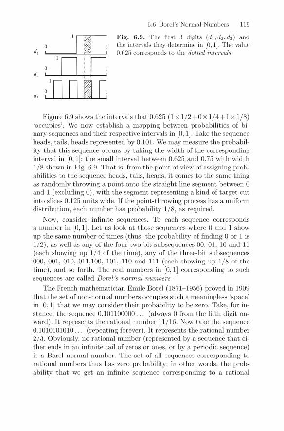
6.6 Borel’s Normal Numbers 119
Fig. 6.9. The first 3 digits (d1, d2, d3) andthe intervals they determine in [0, 1]. The value0.625 corresponds to the dotted intervals
Figure 6.9 shows the intervals that 0.625 (1×1/2+0×1/4+1×1/8)‘occupies’. We now establish a mapping between probabilities of bi-nary sequences and their respective intervals in [0, 1]. Take the sequenceheads, tails, heads represented by 0.101. We may measure the probabil-ity that this sequence occurs by taking the width of the correspondinginterval in [0, 1]: the small interval between 0.625 and 0.75 with width1/8 shown in Fig. 6.9. That is, from the point of view of assigning prob-abilities to the sequence heads, tails, heads, it comes to the same thingas randomly throwing a point onto the straight line segment between 0and 1 (excluding 0), with the segment representing a kind of target cutinto slices 0.125 units wide. If the point-throwing process has a uniformdistribution, each number has probability 1/8, as required.
Now, consider infinite sequences. To each sequence correspondsa number in [0, 1]. Let us look at those sequences where 0 and 1 showup the same number of times (thus, the probability of finding 0 or 1 is1/2), as well as any of the four two-bit subsequences 00, 01, 10 and 11(each showing up 1/4 of the time), any of the three-bit subsequences000, 001, 010, 011,100, 101, 110 and 111 (each showing up 1/8 of thetime), and so forth. The real numbers in [0, 1] corresponding to suchsequences are called Borel’s normal numbers.
The French mathematician Emile Borel (1871–1956) proved in 1909that the set of non-normal numbers occupies such a meaningless ‘space’in [0, 1] that we may consider their probability to be zero. Take, for in-stance, the sequence 0.101100000 . . . (always 0 from the fifth digit on-ward). It represents the rational number 11/16. Now take the sequence0.1010101010 . . . (repeating forever). It represents the rational number2/3. Obviously, no rational number (represented by a sequence that ei-ther ends in an infinite tail of zeros or ones, or by a periodic sequence)is a Borel normal number. The set of all sequences corresponding torational numbers thus has zero probability; in other words, the prob-ability that we get an infinite sequence corresponding to a rational

120 6 Fortune and Ruin
number when playing heads–tails is zero. On the other hand, since theset of all normal numbers has probability 1, we may then say that prac-tically all real numbers in [0, 1] are normal (once again, a result thatmay seem contrary to common intuition). Yet, it has been found to bea difficult task to prove that a given number is normal. Are the deci-mal expansions of
√2, e or π normal? No one knows (although there
is some evidence that they are). A few numbers are known to be nor-mal. One of them, somewhat obvious, was presented by the economistDavid Champernowne (1920–2000) and corresponds to concatenatingthe distinct binary blocks of length 1, 2, 3, etc.:
0.0100011011000001010011100101110111 . . . .
The so-called Copeland–Erdos constant
0.235 711 131 719 232 931 373 941 . . . ,
obtained by concatenating the prime numbers, is also normal in thebase 10 system.
We end with another amazing result. It is well known that the setof all infinite 0–1 sequences is uncountable; that is, it is not possibleto establish a one-to-one mapping between these sequences and thenatural numbers. Well, although the set of non-normal numbers haszero probability, it is also uncountable!
6.7 The Strong Law of Large Numbers
Let us look at sequences of n zeros and ones as coin tosses, denotingby f the frequency of occurrence of 1. The normal numbers satisfy, bydefinition, the following property:
P (limit of the deviation of f from 1/2 is 0) = 1 .
This result is a particular case of a new version of the law of largenumbers. In Chap. 3, the Bernoulli law of large numbers stated that
limit of P (deviation is below t) = 1 ,
where the term ‘deviation’ refers to the absolute value of the differencebetween the average and the expectation (1/2, for coin throwing), asalready pointed out in the last section. The new law, demonstrated bythe Russian mathematician Andrei Kolmogorov (1903–1987) in 1930(more than two centuries after the Bernoulli law), is stated as follows:

6.8 The Law of Iterated Logarithms 121
Fig. 6.10. Convergence conditions for the weak law (a) and the strong law(b) of large numbers
P (limit of the deviation is 0) = 1 .
Let us examine the difference between the two formulations usingFig. 6.10, which displays several deviation curves as a function of n,with t the tolerance of the deviations. In the first version, illustrated inFig. 6.10a, the probability of a deviation larger than t must convergeto 0; that is, once we have fixed the tolerance t (the gray band), we findfewer curves above t as we proceed toward larger values of n. In the caseof Fig. 6.10a, there are three curves above t at n0, two at n1 and oneat n2. The law says nothing about the deviation values. In Fig. 6.10a,the deviation at n2 is even more prominent than the deviation at n1.In the second version of the law, in order for the limit of the average toequal the limit of the expectation with high probability, large wander-ings above any preselected t must become less frequent each time, asFig. 6.10b is intended to illustrate. An equivalent formulation consistsin saying that, in the worst case – the dotted line in Fig. 6.10b – theprobability of exceeding t converges to zero. Thus, the second version ofthe law of large numbers imposes a stronger restriction on the behaviorof the averages than the first version. It is thus appropriate to call itthe strong law of large numbers. The Bernoulli law is then the weaklaw . Understanding the laws of large numbers is an essential prerequi-site to understanding the convergence properties of averages of chancesequences.
6.8 The Law of Iterated Logarithms
We spoke of the central limit theorem in Chap. 4, which allowed us tocompute the value of n above which there is a high certainty of obtain-ing a frequency close to the corresponding probability value. We werethus able to determine that, when p = 1/2 (the coin-tossing example),

122 6 Fortune and Ruin
only after 10 000 throws was there a risk of at most 5% that the f±0.01confidence interval was not typical, i.e., did not contain the true valueof p. On the other hand, the strong law of large numbers shows us thatthere is an almost sure convergence of f toward p. How fast is thatconvergence? Take a sequence of experiments with only two possibleoutcomes, as in the coin-tossing example, and denote the probabilityof one of the outcomes by p. Let S(n) be the accumulated gain after noutcomes and consider the absolute value of the discrepancy betweenS(n) and its expectation, which we know to be np (binomial law).Now, the Russian mathematician Alexander Khintchine demonstratedthe following result in 1924:
P (limit, in the worst case, of a√
2npq log(log n
)deviation) = 1 .
Note that the statement is formulated in terms of a worst case deviationcurve as in Fig. 6.10b. This result, known as the theorem of iteratedlogarithms (the logarithm is repeated), allows one to conclude that f =S(n)/n will almost certainly be between p plus or minus a deviation of√
2pq log(log n
)/n, where ‘almost certainly’ means that, if we add an
infinitesimal increase to that quantity, only a finite subset of all possibleinfinite sequences will deviate by more than that quantity. For instance,for 10 000 throws of a coin we are almost sure that all sequences will
deviate by less than√
0.5 log(log 10 000
)/10 000 = 0.0105.
Figure 6.11 shows 50 sequences of 10 000 throws of a coin withthe deviation of the iterated logarithm (black curves). Note how, af-ter 10 000 throws, practically all curves are inside 0.5 plus or minus
Fig. 6.11. Frequen-cies of heads or tailsin 50 sequences of10 000 throws ofa coin, with the de-viation of the stronglaw
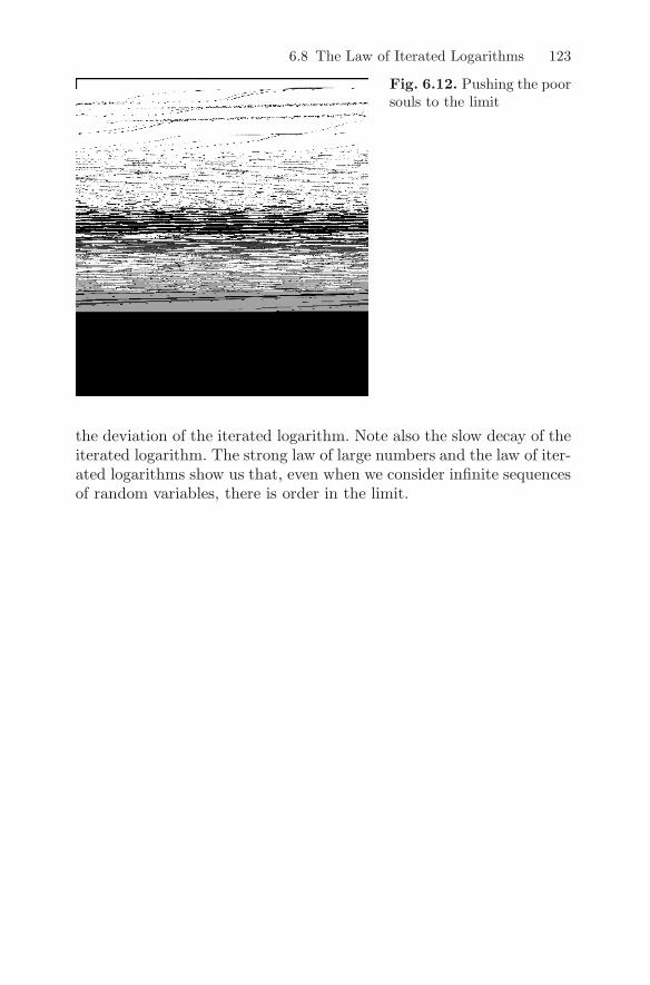
6.8 The Law of Iterated Logarithms 123
Fig. 6.12. Pushing the poorsouls to the limit
the deviation of the iterated logarithm. Note also the slow decay of theiterated logarithm. The strong law of large numbers and the law of iter-ated logarithms show us that, even when we consider infinite sequencesof random variables, there is order in the limit.


7
The Nature of Chance
7.1 Chance and Determinism
The essential property characterizing chance phenomena is the impos-sibility of predicting any individual outcome. When we toss a fair dieor a fair coin in a fair way we assume that that condition is fulfilled.We assume the impossibility of predicting any individual outcome. Theonly thing we may perhaps be able to tell with a given degree of cer-tainty, based on the laws of large numbers, is the average outcome aftera large number of experiments. Yet one might think that it would bepossible in principle to predict any individual outcome. If one knewall the initial conditions of motion, either of the die or of the coin, to-gether with the laws of motion, one might think it possible to forecastthe outcome. Let us look at the example of the coin. The initial con-ditions that would have to be determined are the force vector appliedto the coin, the position of its center of gravity relative to the ground,the shape of the coin and its orientation at the instant of throwing, theviscosity of the air, the value of the acceleration due to gravity at theplace of the experiment, and the friction and elasticity factors of theground. Once all these conditions are known, writing and solving therespective motion equations would certainly be a very complex task,although not impossible. The problem is thus deterministic. Every as-pect of the problem (coin fall, coin rebound, motion on the ground withfriction, etc.) obeys perfectly defined and known laws.
At the beginning of the twentieth century there was a general convic-tion that the laws of the universe were totally deterministic. Probabilitytheory was considered to be a purely mathematical trick allowing usto deal with our ignorance of the initial conditions of many phenom-

126 7 The Nature of Chance
ena. According to Pierre-Simon Laplace in his treatise on probabilitytheory:
If an intelligence knew at a given instant all the forces animat-ing matter, as well as the position and velocity of any of itsmolecules, and if moreover it was sufficiently vast to submitthese data to analysis, it would comprehend in a single formulathe movements of the largest bodies of the Universe and thoseof the tiniest atom. For such an intelligence nothing would beirregular, and the curve described by an air or vapor moleculewould appear to be governed in as precise a way as is for usthe course of the Sun. But due to our ignorance of all the dataneeded for the solution of this grand problem, and the impos-sibility, due to our limited abilities, of subjecting most of thedata in our possession to calculation, even when the amount ofdata is very limited, we attribute the phenomena that seem tous to occur and succeed without any particular order to change-able and hidden causes, whose action is designated by the wordchance, a word that after all is only the expression of our igno-rance. Probability relates partly to this ignorance and in otherparts to our knowledge.
The development of quantum mechanics, starting with the pioneeringwork of the physicists Max Planck (research on black body radiation,which established the concept of the emission of discrete energy quan-tities, or energy quanta), Albert Einstein (research on the photoelectriceffect, establishing the concept of photons as light quanta) and Louisde Broglie (dual wave–particle nature of the electron), at the beginningof the twentieth century, came to change the Laplacian conception ofthe laws of nature, revealing the existence of many so-called quantumphenomena whose probabilistic description is not simply the result ofresorting to a comfortable way of dealing with our ignorance about theconditions that produced them. For quantum phenomena the proba-bilistic description is not just a handy trick, but an absolute necessityimposed by their intrinsically random nature. Quantum phenomena are‘pure chance’ phenomena.
Quantum mechanics thus made the first radical shift away fromthe classical concept that everything in the universe is perfectly de-termined. However, since quantum phenomena are mainly related toelementary particles, i.e., microscopic particles, the conviction that, inthe case of macroscopic phenomena (such as tossing a coin or a die), theprobabilistic description was merely a handy way of looking at things

7.1 Chance and Determinism 127
and that it would in principle be possible to forecast any individualoutcome, persisted for quite some time. In the middle of the twentiethcentury several researchers showed that this concept would also have tobe revised. It was observed that in many phenomena governed by per-fectly deterministic laws, there was in many circumstances such a highsensitivity to initial conditions that one would never be able to guar-antee the same outcome by properly adjusting those initial conditions.However small a deviation from the initial conditions might be, it couldsometimes lead to an unpredictably large deviation in the experimentaloutcomes. The only way of avoiding such disorderly behavior would beto define the initial conditions with infinite accuracy, which amountsto an impossibility. Moreover, it was observed that much of this be-havior, highly sensitive to initial conditions, gave birth to sequences ofvalues – called chaotic orbits – with no detectable periodic pattern. Itis precisely this chaotic behaviour that characterizes a vast number ofchance events in nature. We can thus say that chance has a threefoldnature:
• A consequence of our incapacity or inability to take into accountall factors that influence the outcome of a given phenomenon, eventhough the applicable laws are purely deterministic. This is the coin-tossing scenario.
• A consequence of the extreme sensitivity of many phenomena tocertain initial conditions, rendering it impossible to forecast futureoutcomes, although we know that the applicable laws are purelydeterministic. This is the nature of deterministic chaos which ismanifest in weather changes, for instance.
• The intrinsic random nature of phenomena involving microscopicparticles, which are described by quantum mechanics. Unlike thepreceding cases, since the random nature of quantum phenomenais an intrinsic feature, the best that one can do is to determine theprobability of a certain outcome.
In what follows we first focus our attention on some amazing aspectsof probabilistic descriptions of quantum mechanics. We then proceedto a more detailed analysis of deterministic chaos, which plays a rolein a vast number of macroscopic phenomena in everyday life.

128 7 The Nature of Chance
7.2 Quantum Probabilities
The description of nature at extremely small scales, as is the case ofphotons, electrons, protons, neutrons and other elementary particles,is ruled by the laws of quantum mechanics. Such particles are generi-cally named quanta. There is a vast popular science literature on thistopic (a few indications can be found in the references), describing inparticular the radical separation between classical physics, where lawsof nature are purely deterministic, and quantum mechanics where lawsof nature at a sufficiently small, microscopic, scale are probabilistic. Inthis section we restrict ourselves to outlining some of the more remark-able aspects of the probabilistic descriptions of quantum mechanics(now considered to be one of the best validated theories of physics).
A first remarkable feature consists in the fact that, for a given mi-croscopic system, there are variables whose values are objectively unde-fined. When the system undergoes a certain evolution, with or withouthuman intervention, it is possible to obtain values of these variableswhich only depend on purely random processes: objective, pure, ran-domness. More clearly, the chance nature of the obtained outcome doesnot depend on our ignorance or on incomplete specifications as is thecase for chaotic phenomena. In quantum mechanics, event probabilitiesare objective.
An experiment illustrating the objective nature of chance in quan-tum mechanics consists in letting the light of an extremely weak lightsource fall upon a photographic plate, for a very short time. Supposethat some object is placed between the light source and the plate. Sincethe light intensity is extremely weak, only a small number of photonsfalls on the plate, which will then reveal some spots distributed ina haphazard way around the photographed object. If we repeat theexperiment several times the plates will reveal different spot patterns.Moreover, it is observed that there is no regularity in the process, aswould happen for instance if the first half of the photons impactingthe plate were to do so in the middle region and the other half at theedges. The process is genuinely random. On the other hand, if we com-bine the images of a large number of plates, the law of large numberscomes into play and the image (silhouette) of the photographed objectthen emerges from a ‘sequence of chance events’. It is as though wehad used a Monte Carlo method as a way of defining the contour ofthe object, by throwing tiny points onto the plate.
One strange aspect of quantum mechanics lies in the fact that cer-tain properties of a microscopic particle, such as its position, are char-

7.2 Quantum Probabilities 129
acterized by a probability wave (described by the famous wave equationdiscovered by the Austrian physicist Erwin Schrodinger in 1926). Wecannot, for instance, say at which point a given particle is at a giveninstant. In the absence of a measurement there is a non-null probabilitythat the particle is ‘positioned’ at several points at the same time. Wewrite ‘positioned’ between quotes because in fact it does not have theusual meaning; it really is as though the particle were ‘smeared out’in space, being present partly ‘here’, with a certain probability, andpartly ‘there’, with another probability. The particle is said to be ina superposition state. This superposition state aspect and the wave na-ture, and therefore vector nature of the quantum description, give riseto counterintuitive results which are impossible to obtain when dealingwith uncertainties in everyday life, such as the outcomes of games, fore-casts in the stock market, weather forecasts, and so on, characterizedby a scalar probability measure.
There is a much discussed experiment, the two-slit experiment, thatillustrates the strange behavior of the probabilistic vector nature ofquantum phenomena. A narrow beam of light shines on a target, sepa-rated from the light source by a screen with two small holes (or slits),as shown in Fig. 7.1.
Let us interpret the experiment as in Chap. 4 for the example ofshooting at a target, treating the photons like tiny bullets. With thisassumption the probability of a certain target region being hit by a bul-let is the sum of the probabilities for each of the two possible bullettrajectories; either through A or through B. We may even assume a nor-mal probability density for each of the two possible trajectories, as inFig. 7.1a. In any small region of the target the bullet-hit probabilityis the sum of the probabilities corresponding to each of the normal
Fig. 7.1. Probability density functions in the famous two-slit experiment. (a)According to classical mechanics. (b) What really happens

130 7 The Nature of Chance
distributions. Thus, the probability density of the impact due to thetwo possible trajectories is obtained as the sum of the two densities,shown with a dotted line in Fig. 7.1a. This would certainly be theresult with macroscopic bullets. Now, that is not what happens withphotons, where a so-called interference phenomenon like the one shownin Fig. 7.1b is observed, with concentric rings of smaller or larger lightintensity than the one corresponding to a single slit. This result canbe explained in the framework of classical wave theory. Quantum the-ory also explains this phenomenon by associating a probability wave toeach photon.
In order to get an idea as to how the calculations are performed, wesuppose that an arrow (vector) is associated with each possible trajec-tory of a photon, with the base of the arrow moving at the speed of lightand its tip rotating like a clock hand. At a given trajectory point theprobability of finding the photon at that point is given by the squareof the arrow length. Consider the point P. Figure 7.1b shows two ar-rows corresponding to photon trajectories passing simultaneously (!)through A and B; this is possible due to the state superposition. Whenarriving at P, the clock hands exhibit different orientations, asymmetricin relation to the horizontal bearing, since the lengths of the trajecto-ries FAP and FBP are different. The total probability is obtained asfollows: the two arrows are added according to the parallelogram rule(the construction illustrated in Fig. 7.1b), and the arrow ending at S isobtained as a result. The square of the length of the latter arrow corre-sponds to the probability of an impact at P. At the central point Q, thearrows corresponding to the two trajectories come up with symmetricangles around the horizontal bearing, since the lengths of FAQ andFBQ are now equal. Depending on the choice of the distance betweenthe slits, one may obtain arrows with the same bearing but opposite di-rections, which cancel each other when summing. There are also points,such as R, where the arrows arrive in a concordant way and the lengthof the sum arrow is practically double the length of each vector. It isthen possible to observe null probabilities and probabilities that arefour times larger than those corresponding to a single slit. We thusarrive at the surprising conclusion that the quantum description doesnot always comply with
P (passing through A or passing through B)
= P (passing through A) + P (passing through B) ,
as would be observed in a classical description!

7.2 Quantum Probabilities 131
What happens when a single photon passes through a single slit?Does it smear out in the target as a blot with a bell-shaped intensity?No. The photon ends at an exact (but unknown) point. The bell-shapedblot is a result of the law of large numbers. There is no intrinsic featuredeciding which photons hit the center and which ones hit the periphery.The same applies to the interference phenomenon. Only the probabilis-tic laws that govern the phenomena are responsible for the final result.Incidentally, if we place photon detectors just after the two slits A andB, the interference phenomenon no longer takes place. Now, by actingwith a detector, the state superposition is broken and we can say whichslit a given photon has passed through.
The interference phenomenon has also been verified experimentallywith other particles of reduced dimensions such as electrons, atoms, andeven with larger molecules, as in recent experiments with the buckmin-sterfullerene molecule, composed of 60 carbon atoms structured likea football.
Another class of experiments illustrating the strangeness of quan-tum probabilities relates to properties of microscopic particles exhibit-ing well defined values. It is a known fact that light has a wave nature aswell as a particle nature, represented by the oscillation of an electromag-netic field propagating as a wave, with the electric field vector vibratingperpendicularly to the propagation direction. Common light includesmany wave components with various vibration directions, called polar-izations. However, with the help of a polarizing device (for instance,a sheet of a special substance called polaroid or a crystal of the min-eral calcite), one may obtain a single light component with a specificdirection of polarization.
In Fig. 7.2b, horizontally polarized light (the electric field vibratesperpendicularly to the page), denoted by h, shines on a polarizer whosedirection of polarization makes a 45-degree angle with the horizontal
Fig. 7.2. (a) Polarization directions in a plane perpendicular to the propaga-tion direction. (b) Horizontally polarized light passing through two polaroids.(c) As in (b) but in the opposite order

132 7 The Nature of Chance
direction (see Fig. 7.2a). Let Eh be the electric field intensity of h.The intensity coming out of the 45 polarizer corresponds to the fieldprojection along this direction, that is,
E1 = Eh cos 45 =Eh√
2.
The light passes next through a vertical polarizer (the electric fieldvibrates in the page perpendicularly to the direction of propagation),and likewise
E2 = E1 sin 45 =E1√
2=
Eh
2.
Let us now suppose that we change the order of the polarizers as inFig. 7.2c. We obtain
E1 = Eh cos 90 = 0 ,
hence, E2 = 0. These results, involving electric field projections alongpolarization directions, are obvious in the framework of the classicalwave theory. Let us now interpret them according to quantum mechan-ics. In fact, light intensity, which is proportional to the square of theelectric field amplitude, measures the probability of a photon passingthrough the two-polarizer sequence. But we thus arrive at the conclu-sion, contrary to common sense, that in the quantum description theprobabilities of a chain of events are not always commutative, inde-pendent of the order of events, since the probability associated withthe experimental result of Fig. 7.2b is different from the one associatedwith Fig. 7.2c. Suppose that instead of light we had a flow of sandgrains passing through a sequence of two sieves: sieve 1 and sieve 2. Inthe classical description, the commutative property holds:
P (passing through sieve 1) × P
(passing through sieve 2
if it has passed through sieve 1
)
= P (passing through sieve 2) × P
(passing through sieve 1
if it has passed through sieve 2
)
.
In the quantum description the probability of the intersection dependson the order of the events! This non-commutative feature of quantumprobabilities has also been observed in many other well-defined prop-erties of microscopic particles, such as the electron spin.
The laws of large numbers also come into play in all quantum phe-nomena, as we saw earlier in the case where an object was photographed

7.2 Quantum Probabilities 133
with very weak light. In the interference example, if the source lightonly emits a small number of photons per second, one initially observesa poorly defined interference pattern, but it will begin to build up astime goes by. Another particularly interesting illustration of the law oflarge numbers acting on quantum phenomena is obtained in an experi-ment in which the intensity of a light beam with a certain polarization,say h, is measured after it has passed through a polarizer with polar-ization axis at an angle θ to h. We have already seen that the lightintensity is then proportional to the square of cos θ. In fact, it is pro-portional to the number of photons passing through the polarizer, viz.,Np = N cos2 θ, where N is the number of photons hitting the polar-izer. If we carry out the experiment with a light beam of very weakintensity (in such a way that only a small number of photons hits thepolarizer) and, for each value of θ, we count how many photons passthrough (this can be done with a device called a photomultiplier), weobtain a graph like the one shown in Fig. 7.3. This graph clearly showsrandom deviations in the average number of photons Np/N passingthrough the polarizer from the theoretical value of cos2 θ. An experi-ment with a normal light beam, with very high N , can be interpreted ascarrying out multiple experiments such as the one portrayed in Fig. 7.3.But in this case the law of large numbers comes into play, and in sucha way that the average number of photons passing through the polar-izer exhibits a standard deviation proportional to 1/
√N (as already
seen in Chap. 4). In summary, for an everyday type of light beam, thelaw of large numbers explains the cos2 θ proportionality, as deduced inthe framework of classical physics for the macroscopic object we calla light beam.
Fig. 7.3. Average numberof photons passing througha polarizer for several polar-izer angles (simulation)

134 7 The Nature of Chance
Another strange aspect of quantum mechanics, which still raisesmuch debate, concerns the transition between a quantum descriptionand a classical description. In other words, when is a particle largeenough to ensure that quantum behavior is no longer observed? Themodern decoherence theory presents an explanation consistent withexperimental results, according to which for sufficiently large particles,where sufficient means that an interaction with other particles in thesurrounding space is inevitable, the state superposition is no longerpreserved.
The intrinsically random nature of quantum phenomena was a sourceof embarrassment for many famous physicists. It was even suggestedthat instead of probability waves, there existed in the microscopic par-ticles some internal variables, called hidden variables, that were de-terministically responsible for quantum phenomena. However, a resultdiscovered in 1964 by the physicist John Bell (known as Bell’s theo-rem) proved that no theory of local hidden variables would be able toreproduce in a consistent way the probabilistic outcomes of quantummechanics. The random nature of quanta is therefore the stronghold oftrue randomness, of true chance. Quanta are the quintessential chancegenerators, putting dice, coins and the like to shame.
7.3 A Planetary Game
Playing dice in space may not be a very entertaining activity. In weight-less conditions, astronauts would see the dice floating in the air, withoutmuch hope of deciding what face to read off. Imagine a space game forastronauts, using balls instead of dice, and making use of the weightlessconditions in order to obtain orbital ball trajectories. One of the balls,of largest mass, plays the role of the Sun in a mini-planetary system.In this planetary game two balls are used, playing the role of planetswith co-planar orbits.
Let us first take a single planet P1 and to fix ideas let us supposethat the Sun and planet have masses 10 kg and 1 kg, respectively. Themass of the planet is reasonably smaller than the mass of the Sun sothat its influence on the Sun’s position can be neglected. We may thenconsider that the Sun is fixed at the point (0, 0) of a coordinate sys-tem with orthogonal axes labelled x and y in the orbital plane. If anastronaut places P1 1.5 m away from the Sun with an initial velocityof 7 cm/hr along one of the orthogonal directions, (s)he will be able toconfirm the universal law of gravitation, observing P1 moving round ina slightly elliptic orbit with an orbital period of about 124 hr (assuming

7.3 A Planetary Game 135
that the astronaut is patient enough). We now suppose that a secondplanet P2, also with mass 1 kg, is placed farther away from the Sunthan P1 and with an initial velocity of 6 cm/hr along one of the orthog-onal directions. The game consists in predicting where (to within sometolerance) one of the planets can be found after a certain number ofhours. If P2 is placed at an initial distance of r = 3 m from the Sun, weget the stable orbit situation shown in Fig. 7.4a and the position of theplanets is predictable. In this situation a slight deviation in the positionof P2 does not change the orbits that much, as shown in Fig. 7.4b. Onthe other hand, if P2 is placed 2 m from the Sun, we get the chaoticorbits shown in Fig. 7.5a and the positions of the planets can no longerbe predicted. Even as tiny a change in the position as an increment of0.00000001 m (a microbial increment!) causes a large perturbation, asshown in Fig. 7.5b. One cannot even predict the answer to such a simplequestion as: Will P1 have made an excursion beyond 3 m after 120 hr?Faced with such a question, the astronauts are in the same situationas if they were predicting the results of a coin-tossing experiment.
The chaotic behavior of this so-called three-body problem was firststudied by the French mathematician Jules Henri Poincare (1854–1912), pioneer in the study of chaotic phenomena. Poincare and otherresearchers have shown that, by randomly specifying the initial con-ditions of three or more bodies, the resulting motion is almost alwayschaotic, in contrast to what happens with two bodies, where the motionis never chaotic. For three or more bodies no one can tell, in general,which trajectories they will follow. This is the situation with certain
Fig. 7.4. Stable orbits of the planets, with the ‘Sun’ at (0, 0). (a) r = 3 m.(b) r = 3.01 m

136 7 The Nature of Chance
Fig. 7.5. Chaotic orbits of the planets, with the ‘Sun’ at (0, 0). (a) r = 2 m.(b) r = 2.000 000 01 m
asteroids. The problem can only be treated for certain specific sets ofconditions. In the following sections, we shall try to cast some light onthe nature of these phenomena.
7.4 Almost Sure Interest Rates
Consider the calculation of accumulated capital after n years, in a cer-tain bank with an annual constant interest rate of j. Assume an initialcapital, denoted by C0, of 1 000 euro, and an interest rate of 3% peryear. After the first year the accumulated capital C1 is
C1 = C0 + C0 × j = 1000 + 1000 × 0.03 = C0 × 1.03 .
After the second year we get in the same way, C2 = C1 × 1.03 =C0 × 1.032. Thus, after n years, iteration of the preceding rule showsthat the capital is Cn = C0 × 1.03n.
After carrying out the computations with a certain initial capital C0,suppose we came to the conclusion that its value was wrong and weshould have used C0 +E0. For instance, instead of 1 000 euro we shouldhave used 1 001 euro, corresponding to a relative error of E0/C0 =1/1 000. Do we have to redo all calculations or is there a simple rulefor determining how the initial E0 = 1 euro error propagates after nyears? Let us see. After the first year the capital becomes
C0 × 1.03 + E0 × 1.03 .
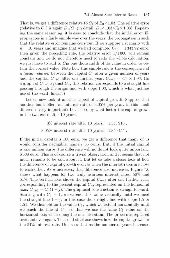
7.4 Almost Sure Interest Rates 137
That is, we get a difference relative to C1 of E0×1.03. The relative error(relative to C1) is again E0/C0 (in detail, E0×1.03/C0×1.03). Repeat-ing the same reasoning, it is easy to conclude that the initial error E0
propagates in a fairly simple way over the years: the propagation is suchthat the relative error remains constant . If we suppose a scenario withn = 10 years and imagine that we had computed C10 = 1343.92 euro,then given the preceding rule, the relative error 1/1 000 will remainconstant and we do not therefore need to redo the whole calculation;we just have to add to C10 one thousandth of its value in order to ob-tain the correct value. Note how this simple rule is the consequence ofa linear relation between the capital Cn after a given number of yearsand the capital Cn+1 after one further year: Cn+1 = Cn × 1.03. (Ina graph of Cn+1 against Cn, this relation corresponds to a straight linepassing through the origin and with slope 1.03, which is what justifiesuse of the word ‘linear’.)
Let us now look at another aspect of capital growth. Suppose thatanother bank offers an interest rate of 3.05% per year. Is this smalldifference very important? Let us see by what factor the capital growsin the two cases after 10 years:
3% interest rate after 10 years: 1.343 916 ,
3.05% interest rate after 10 years: 1.350 455 .
If the initial capital is 100 euro, we get a difference that many of uswould consider negligible, namely 65 cents. But, if the initial capitalis one million euros, the difference will no doubt look quite important:6 538 euro. This is of course a trivial observation and it seems that notmuch remains to be said about it. But let us take a closer look at howthe difference of capital growth evolves when the interest rates are closeto each other. As n increases, that difference also increases. Figure 7.6shows what happens for two truly usurious interest rates: 50% and51%. The vertical axis shows the capital Cn+1 after one further year,corresponding to the present capital Cn, represented on the horizontalaxis: Cn+1 = Cn(1 + j). The graphical construction is straightforward.Starting with C0 = 1, we extend this value vertically until we meetthe straight line 1 + j, in this case the straight line with slope 1.5 or1.51. We thus obtain the value C1, which we extend horizontally untilwe reach the line at 45, so that we use the same C1 value on thehorizontal axis when doing the next iteration. The process is repeatedover and over again. The solid staircase shows how the capital grows forthe 51% interest rate. One sees that as the number of years increases

138 7 The Nature of Chance
Fig. 7.6. Capital growthfor (usurious!) interest rates:50% and 51%
(see Fig. 7.6) the difference between the two capital growth factorsincreases in proportion to the number of years. In fact, Fig. 7.6 clearlyillustrates that the difference in values of the capital is proportional ton, i.e., changes linearly with n. For the 3% and 3.05% interest rates,the difference in values of the capital varies with n as a straight linewith slope (0.030 5 − 0.03)/1.03 = 0.000 485 per year.
This linearly growing difference in capital for distinct (and constant)interest rates is also well known. However, what most people do not re-alize is that numerical computations are always performed with finiteaccuracy . That is, it does not matter how the calculations are carriedout, e.g., by hand or by computer, the number of digits used in thenumerical representation is necessarily finite. Therefore, the results aregenerally approximate. For instance, we never get exact calculationsfor an interest rate of 1/30 per year, since 1/30 = 0.033 333 3 . . . (con-tinuing infinitely).
Banks compute accumulated capitals with computers. These mayuse different numbers of bits in their calculations, corresponding to dif-ferent numbers of decimal digits. Personal computers usually performthe calculations using 32 bits (the so-called simple precision represen-tation, equivalent to about 7 significant decimal digits) and in 64 bits(the so-called double precision representation, equivalent to about 15significant decimal digits). Imagine a firm deciding to invest one millioneuros in a portfolio of shares with an 8% annual interest rate. Apply-ing this constant 8% interest rate the firm’s accountant calculates theaccumulated capital on the firm’s computer with 32-bit precision. Thebank performs the same calculation but with 64-bit precision. Theycompare their calculations and find that after 25 years there is a 41

7.5 Populations in Crisis 139
Fig. 7.7. Annualevolution of the dif-ference of accumu-lated capital com-puted by two differ-ent computers
cent difference in an accumulated capital of about six million eighthundred thousand euros. In order to clear up this issue they comparethe respective calculations for a 50-year period and draw the graph ofthe differences between the two calculations, as in Fig. 7.7. After 50years the difference is already 6.51 euro. Moreover, they verify thatthe difference does not progress in a systematic, linear way; it showschaotic fluctuations that are difficult to forecast. If there is a notice-able difference when using a 64-bit computer, why not use a 128-bitor a 256-bit computer instead? In fact, for problems where numericalprecision is crucial one may use supercomputers that allow a very largenumber of bits for their computations. But the bottom line is this: nomatter how super the computer is, we will always have to deal withuncertainty factors in our computations due to the finite precision ofnumber representation and error propagation. In some cases the men-tioned uncertainty is insignificant (the firm would probably not paymuch attention to a 41 cent difference in six million eight hundredthousand euros). In other cases error propagation can have dramaticconsequences.
7.5 Populations in Crisis
In the above interest rate problem, the formula Cn+1 = Cn(1 + j) forcapital growth is a linear formula, i.e., Cn+1 is directly proportional toCn. This linear dependency is reflected in the well-behaved evolutionof the capital growth for a small ‘perturbation’ of the initial capital.Unfortunately, linear behavior is more the exception than the rule,either in natural phenomena or in everyday life.
We now consider a non-linear phenomenon, relating to the evolutionof the number of individuals in a population after n time units. Let usdenote the number of individuals by Nn and let N be the maximum

140 7 The Nature of Chance
reference value allowed by the available food resources. We may, forinstance, imagine a population of rabbits living inside a fenced field.If our time unit is the month, we may further assume that after threemonths we have N3 = 60 rabbits living in a field that can only supportup to N = 300 rabbits. Let Pn = Nn/N denote the fraction of themaximum number of individuals that can be supported by the availableresources. For the above-mentioned values, we have P3 = 0.2. If thepopulation grew at a constant rate r, we would get a situation similarto the one for the interest rate: Pn+1 = Pn(1 + r). However, with anincreasing population, the necessary resources become scarcer and onemay reach a point where mortality overtakes natality owing to lack ofresources; Pn will then decrease. A formula reflecting the need to imposea growth rate that decreases as one approaches a maximum number ofindividuals, becoming a dwindle rate if the maximum is exceeded, is
Pn+1 = Pn
[1 + r(1 − Pn)
].
According to this rule the population grows or dwindles at the rate ofr(1−Pn). If Pn is below 1 (the Pn value for the population maximum),the population grows, and all the more as the deviation from the max-imum is greater. As soon as Pn exceeds 1, a dwindling phase sets in.Note that the above formula can be written as Pn+1 = Pn(1+r)−rP 2
n ,clearly showing a non-linear, quadratic, dependency of Pn+1 on Pn.
Suppose we start with P0 = 0.01 (one per cent of the referencemaximum) and study the population evolution for r = 1.9. We findthat the population keeps on growing until it stabilizes at the maximum(Fig. 7.8a). If r = 2.5, we get an oscillating pattern (Fig. 7.8b) withperiod 4 (months).
Sometimes the periodic behavior is more complex than the one inFig. 7.8b. For instance, in the case of Fig. 7.9, the period is 32 and ittakes about 150 time units until a stable oscillation is reached. If weset a 0.75 threshold, as in Fig. 7.9, interpreting as 1 the values abovethe threshold and as 0 the values below, we get the following periodicsequence:
111010101110101011101010111011101110101011101010111 . . .
But strange things start to happen when r approaches 3. For r = 3and P0 = 0.1, we get the behavior illustrated in Fig. 7.10a. A very tinyerror in the initial condition P0, for instance P0 = 0.100 001, is enoughto trigger a totally different evolution, as shown in Fig. 7.10b.
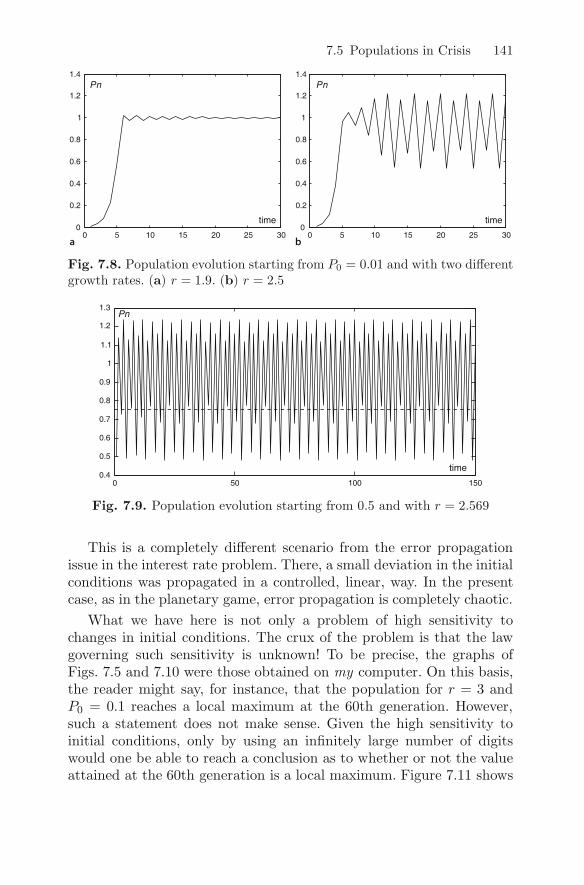
7.5 Populations in Crisis 141
Fig. 7.8. Population evolution starting from P0 = 0.01 and with two differentgrowth rates. (a) r = 1.9. (b) r = 2.5
Fig. 7.9. Population evolution starting from 0.5 and with r = 2.569
This is a completely different scenario from the error propagationissue in the interest rate problem. There, a small deviation in the initialconditions was propagated in a controlled, linear, way. In the presentcase, as in the planetary game, error propagation is completely chaotic.
What we have here is not only a problem of high sensitivity tochanges in initial conditions. The crux of the problem is that the lawgoverning such sensitivity is unknown! To be precise, the graphs ofFigs. 7.5 and 7.10 were those obtained on my computer. On this basis,the reader might say, for instance, that the population for r = 3 andP0 = 0.1 reaches a local maximum at the 60th generation. However,such a statement does not make sense. Given the high sensitivity toinitial conditions, only by using an infinitely large number of digitswould one be able to reach a conclusion as to whether or not the valueattained at the 60th generation is a local maximum. Figure 7.11 shows

142 7 The Nature of Chance
Fig. 7.10. Chaotic population evolution for r = 3. (a) P0 = 0.1. (b) P0 =0.100 001
Fig. 7.11. Time evolutionof the difference in theFig. 7.10 populations
the difference of Pn values between the evolutions shown in Fig. 7.10. Itis clear that after a certain time no rule allows us to say how the initialperturbation evolves with n. This is the nature of deterministic chaos.In the case of the interest rate, we had no chaos and a very simple rulewas applied to a ‘perturbation’ of the initial capital: the perturbationwas propagated in such a way that the relative differences were keptconstant. In deterministic chaos there are no rules. The best one cando is to study statistically how the perturbations are propagated, onaverage.
7.6 An Innocent Formula
There is a very simple formula that reflects a quadratic dependency ofthe next value of a given variable x relative to its present value. It is
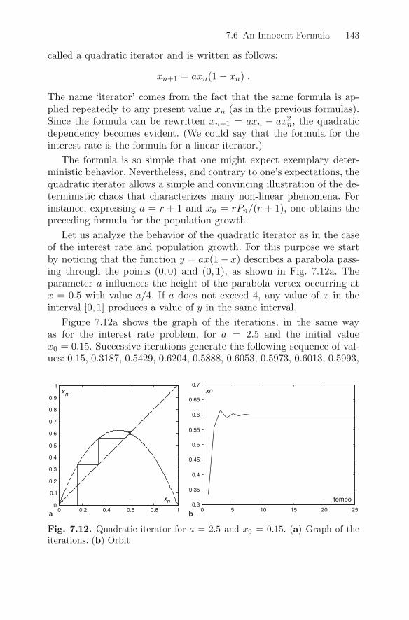
7.6 An Innocent Formula 143
called a quadratic iterator and is written as follows:
xn+1 = axn(1 − xn) .
The name ‘iterator’ comes from the fact that the same formula is ap-plied repeatedly to any present value xn (as in the previous formulas).Since the formula can be rewritten xn+1 = axn − ax2
n, the quadraticdependency becomes evident. (We could say that the formula for theinterest rate is the formula for a linear iterator.)
The formula is so simple that one might expect exemplary deter-ministic behavior. Nevertheless, and contrary to one’s expectations, thequadratic iterator allows a simple and convincing illustration of the de-terministic chaos that characterizes many non-linear phenomena. Forinstance, expressing a = r + 1 and xn = rPn/(r + 1), one obtains thepreceding formula for the population growth.
Let us analyze the behavior of the quadratic iterator as in the caseof the interest rate and population growth. For this purpose we startby noticing that the function y = ax(1 − x) describes a parabola pass-ing through the points (0, 0) and (0, 1), as shown in Fig. 7.12a. Theparameter a influences the height of the parabola vertex occurring atx = 0.5 with value a/4. If a does not exceed 4, any value of x in theinterval [0, 1] produces a value of y in the same interval.
Figure 7.12a shows the graph of the iterations, in the same wayas for the interest rate problem, for a = 2.5 and the initial valuex0 = 0.15. Successive iterations generate the following sequence of val-ues: 0.15, 0.3187, 0.5429, 0.6204, 0.5888, 0.6053, 0.5973, 0.6013, 0.5993,
Fig. 7.12. Quadratic iterator for a = 2.5 and x0 = 0.15. (a) Graph of theiterations. (b) Orbit

144 7 The Nature of Chance
0.6003, 0.5998, and so on. This sequence, converging to 0.6, is shownin Fig. 7.12b. As in the previous examples we may assume that theiterations occur in time. The graph of Fig. 7.12b is said to representone orbit of the iterator. If we introduce a small perturbation of theinitial value (for instance, x0 = 0.14 or x0 = 0.16), the sequence stillconverges to 0.6.
Figure 7.13 shows a non-convergent chaotic situation for a = 4.A slight perturbation of the initial value produces very different orbits,as shown in Fig. 7.14. Between the convergent case and the chaoticcase the quadratic iterator also exhibits periodic behavior, as we hadalready detected in the population growth model.
Fig. 7.13. Fifteen iterations of the quadratic iterator for a = 4. (a) x0 = 0.2.(b) x0 = 0.199
Fig. 7.14. Quadratic iterator orbits for a = 4. (a) x0 = 0.2. (b) x0 = 0.199999

7.6 An Innocent Formula 145
Now suppose we have divided the [0, 1] interval into small subinter-vals of width 0.01 and that we try to find the frequency with which anyof these subintervals is visited by the quadratic iterator orbit, for a = 4and x0 = 0.2. Figure 7.15 shows what happens after 500 000 iterations.As the number of iterations grows the graph obtained does not changewhen we specify different initial values x0. Interpreting frequencies asprobabilities, we see that the probability of obtaining a visit of a subin-terval near 0 or 1 is rather larger than when it is near 0.5. In fact, itis possible to prove that for infinitesimal subintervals one would obtainthe previously mentioned arcsine law (see Chap. 6) for the frequencyof visits of an arbitrary point. That is, the probability of our chaoticorbit visiting a point x is equal to the probability of the last zero gainhaving occurred before time x in a coin-tossing game!
Consider the following variable transformation for the quadratic it-erator:
xn = sin2(πyn) .
For a = 4, it can be shown that this transformation allows one torewrite the iterator formula as
yn+1 = 2yn (mod 1) ,
where the mod 1 (read modulo 1) operator means removing the integerpart of the expression to which it applies (2yn in this case). The chaoticorbits of the quadratic iterator are therefore mapped onto chaotic orbitsof yn. We may also express the yn value relative to an initial value y0.As in the case of the interest rate, we get
yn = 2ny0 (mod 1) .
Fig. 7.15. Probability ofthe chaotic quadratic itera-tor (a = 4) visiting a subin-terval of [0, 1] of width 0.01,estimated in 500 000 itera-tions

146 7 The Nature of Chance
Let us see what this equation means, by considering y0 expressedin binary numbering, for instance y0 = 0.101 100 100 010 111 1. Inthe first iteration we have to multiply by 2 and remove the integerpart. In binary numbering, multiplying by 2 means a one-bit leftwardshift of the whole number, with a zero carried in at the right (sim-ilarly to what happens when we multiply by 10 in decimal number-ing). We get 1.011 001 000 101 111 0. Removing the integer part we get0.011 001 000 101 111 0. The same operations are performed in the fol-lowing iterations. Suppose we only look at the successive bits of theremoved integer parts. What the iterations of the above formula thenproduce are the consecutive bits of the initial value, which can be in-terpreted as an infinite sequence of coin throws. Now, we already knowthat, with probability 1, a Borel normal number can be obtained byrandom choice in [0, 1]. As a matter of fact, we shall even see in Chap. 9that, with probability 1, an initial value y0 randomly chosen in [0, 1]turns out to be a number satisfying a strict randomness criterion, whosebits cannot be predicted either by experiment or by theory. Chaos al-ready exists in the initial y0 value! The quadratic iterator does not com-pute anything; it only reproduces the bits of y0. The main issue here isnot an infinite precision issue. The main issue is that we do not havea means of producing the bits of the sequence other than having a pre-stored list of them (we shall return to this point in Chap. 9). However,not all equations of the above type produce chaotic sequences, in thesense that they do not propagate chaos to the following iterations. Forinstance, the equation xn+1 = xn +b (mod 1) does not propagate chaosinto the following iteration. We see this because, if x0 and x′
0 are veryclose initial conditions, after n iterations we will get x′
n −xn = x′
0−x0.That is, the difference of initial values continues indefinitely.
7.7 Chance in Natural Systems
Many chance phenomena in natural systems composed of macroscopicobjects are of a chaotic nature. These systems generally involve severalvariables to characterize the state of the system as time goes by, ratherthan one as in the example of population evolution:
• for the 3-sphere system described above, the characterizing variablesare the instantaneous values of two or three components of positionand velocity,
• for a container where certain reagents are poured, the characterizingvariables are the concentrations of reagents and reaction products,

7.7 Chance in Natural Systems 147
• for weather forecasting, the characterizing variables are the pressureand temperature gradients,
• for cell culture evolution the relevant variables may be nutrient andcell concentrations,
• for financial investments, they may be rental rates and other marketvariables,
and so on and so forth.
Let x denote a variable characterizing the system and let xn andxn+1 represent the values at consecutive instants of time, assumedclose enough to each other to ensure that the difference xn+1 − xn
reflects the instantaneous time evolution in a sufficiently accurate way.If these differences vary linearly with xn, no chaotic phenomena takeplace. Chaos in the initial conditions does not propagate. Chaos re-quires non-linearities in order to propagate, as was the case for thequadratic dependence in the population growth example. Now it justhappens that the time evolution in a huge range of natural systemsdepends in a non-linear way on the variables characterizing the sys-tem. Consider the example of a sphere orbiting in the xy plane aroundanother sphere of much larger mass placed at (0, 0). Due to the lawof gravitation, the time evolution of the sphere’s coordinates dependson the reciprocal of its distance
√
x2 + y2 to the center. We thus geta non-linear dependency. In the case of a single orbiting sphere nochaotic behavior will arise. However, by adding a new sphere to thesystem we are adding an extra non-linear term and, as we have seen,chaotic orbits may arise.
The French mathematician Poincare carried out pioneering work onthe time evolution of non-linear systems, a scientific discipline whichhas attracted great interest not only in physics and chemistry, but alsoin the fields of biology, physiology, economics, meteorology and oth-ers. Many non-linear systems exhibit chaotic evolution under certainconditions. There is an extensive popular science literature describingthe topic of chaos, where many bizarre kinds of behavior are presentedand characterized. What interests us here is the fact that a systemwith chaotic behavior is a chance generator (like tossing coins or dice),in the sense that it is not possible to predict the values of the vari-ables. The only thing one can do is to characterize the system variablesprobabilistically.
An example of a chaotic chance generator is given by the thermalconvection of the so-called Benard cells. The generator consists of a thinlayer of liquid between two glass plates. The system is placed over

148 7 The Nature of Chance
a heat source. When the temperature of the plate directly in contactwith the heat source reaches a certain critical value, small domainsare formed in which the liquid layer rotates by thermal convection.These are the so-called Benard cells. The direction of rotation of thecells (clockwise or counterclockwise) is unpredictable and depends onmicroscopic perturbations. From this point of view, one may considerthat the rotational state of a Benard cell is a possible substitute forcoin tossing. If after obtaining the convection cells we keep on raisingthe temperature, a new critical value is eventually reached where thefluid motion becomes chaotic (turbulent), corresponding to an evenmore complex chance generator. Many natural phenomena exhibit somesimilarity with the Benard cells, e.g., meteorological phenomena.
Meteorologists are perfectly familiar with turbulent atmosphericphenomena and with their hypersensitivity to small changes in cer-tain conditions. In fact, it was a meteorologist (and mathematician)Edward Lorenz who discovered in 1956 the lack of predictability ofcertain deterministic systems, when he noticed that weather forecastsbased on certain computer-implemented models were highly sensitiveto tiny perturbations (initially Lorenz mistrusted the computer and re-peated the calculations with several machines!). As Lorenz says in oneof his writings: “One meteorologist remarked that if the theory werecorrect, one flap of a seagull’s wings could change the course of weatherforever.” This high sensitivity to initial conditions afterwards came tobe called the butterfly effect.
The Lorenz equations, which are also applied to the study of con-vection in Benard cells, are
xn+1 − xn = σ(yn − xn) , yn+1 − yn = xn(τ − zn) − yn ,
zn+1 − zn = xnyn − βzn .
In these equations, x represents the intensity of the convective motion,y the temperature difference between ascending and descending fluid,and z the deviation from linearity of the vertical temperature profile.Note the presence of the non-linear terms xnzn and xnyn, responsiblefor chaotic behavior for certain values of the control parameters, asillustrated in Fig. 7.16. This three-dimensional orbit is known as theLorenz attractor.
Progress in other studies of chaotic phenomena has allowed the iden-tification of many other systems of inanimate nature with chaotic be-havior, e.g., variations in the volume of ice covering the Earth, vari-

7.8 Chance in Life 149
Fig. 7.16. Chaotic orbit ofLorenz equations for σ = 10,τ = 28, β = 8/3
ations in the Earth’s magnetic field, river flows, turbulent fluid mo-tion, water dripping from a tap, spring vibrations subject to non-linearforces, and asteroid orbits.
7.8 Chance in Life
While the existence of chaos in inanimate nature may not come asa surprise, the same cannot be said when we observe chaos in nature.In fact, life is ruled by laws that tend to maintain equilibrium of thebiological variables involved, in order to guarantee the development ofmetabolic processes compatible with life itself. For instance, if we havebeen running and we are then allowed to rest, the heart rate whichincreased during the run goes back to its normal value after some time;concomitantly, the energy production mode that was adjusted to suitthe greater muscular requirements falls back into the normal productionmode which prevails in the absence of muscular stress. One then ob-serves that the physiological variables (as well as the biological variablesat cellular level) fall back to the equilibrium situation corresponding toan absence of effort. If on the other hand we were not allowed to restand were instead obliged to run indefinitely, there would come a pointof death by exhaustion, when it would no longer be possible to sustainthe metabolic processes in a way compatible with life.
Life thus demands the maintenance of certain basic balances andone might think that such balances demand a perfectly controlled, non-chaotic, evolution of the physiological and biological variables. Surpris-ingly enough this is not the case. Consider the heart rate of a rest-ing adult human. One might think that the heart rate should stayat a practically constant value or at most exhibit simple, non-chaotic

150 7 The Nature of Chance
fluctuations. However, it is observed that the heart rate of a healthyadult (in fact, of any healthy animal and in any stage of life) exhibitsa chaotic behavior, even at rest, as shown in Fig. 7.17. Heart rate vari-ability is due to two factors: the pacemaker and the autonomic nervoussystem. The pacemaker consists of a set of self-exciting cells in the rightatrium of the heart. It is therefore an oscillator that maintains a practi-cally constant frequency in the absence of stimuli from the autonomicnervous system. The latter is responsible for maintaining certain in-voluntary internal functions approximately constant. Beside the heartbeat, these include digestion, breathing, and the metabolism. Althoughthese functions are usually outside voluntary control they can be influ-enced by the mental state. The autonomic nervous system is composedof two subsystems: the sympathetic and the parasympathetic. The firstis responsible for triggering responses appropriate to stress situations,such as fear or extremes of physical activity. Increase in heart rate isone of the elicited responses. The parasympathetic subsystem is re-sponsible for triggering energy saving and recovery actions after stress.A decrease in heart rate is one of the elicited actions.
The variability one observes in the heart rate is therefore influencedby the randomness of external phenomena causing stress situations.However, it has also been observed that there is a chaotic behavior ofthe heart rate associated with the pacemaker itself, whose causes arenot yet fully understood. (However, some researchers have been ableto explain the mechanism leading to the development of chaotic phe-nomena in heart cells of chicken, stimulated periodically.) Whatever itscauses, this chaotic heart rate behavior attenuates with age, reflectingthe heart’s loss of flexibility in its adaptation to internal and externalstimuli.
Chaotic phenomena can also be observed in electrical impulsestransmitted by nervous cells, the so-called action potentials. An actionpotential is nothing other than an electrical impulse sent by a neuron to
Fig. 7.17. Heartrate of an adult man.The frequency isexpressed in beatsper minute

7.8 Chance in Life 151
Fig. 7.18. Evolution ofsuccessive action potentialsin nervous cells (t0 = 0.1 s,R = 3 s−1)
other neurons. These impulses have an amplitude of about 0.1 volt andlast about 2 milliseconds. Two researchers (Glass and Mackey in 1988)were able to present a deterministic model for the time intervals tnbetween successive peaks of action potentials. The model is non-linearand stipulates that the following inter-peak interval is proportional tothe logarithm of the absolute value of 1− 2e−Rtn , where R is a controlparameter of the model. This model exhibits chaotic behavior of thekind shown in Fig. 7.18 for certain values of the control parameter, andthis behavior has in fact been observed in practice.
Many other physiological phenomena exhibit chaotic behavior, e.g.,electrical potentials in cell membranes, breathing tidal volumes, vascu-lar movements, metabolic phenomena like glucose conversion in adeno-sine triphosphate, and electroencephalographic signals.
Fig. 7.19. Will it work?

8
Noisy Irregularities
8.1 Generators and Sequences
Imagine that you were presented with two closed boxes named C1 andC2, both producing a tape with a sequence of sixteen zeros and oneswhenever a button is pressed. The reader is informed that one of theboxes uses a random generator to produce the tape, while the otherbox uses a periodic generator. The reader’s task is to determine, usingonly the tapes produced by the boxes, which one, C1 or C2, containsthe random generator. The reader presses the button and obtains:
C1 sequence : 0011001100110011 ,
C2 sequence : 1101010111010101 .
The reader then decides that box C2 contains the random generator.The boxes are opened and to the reader’s amazement the random gen-erator is in box C1 (where, for instance, a mechanical device tossesa coin) whereas box C2 contains the periodic generator correspond-ing to Fig. 7.9. This example illustrates the impossibility of decidingthe nature (deterministic or random) of a sequence generator on thebasis of observation, and in fact on the basis of any randomness mea-surement, of one of its sequences (necessarily finite). For the momentthe ‘measure’ is only subjective. The reader decides upon C2 becausethe corresponding sequence looks irregular. Later on, we present a fewobjective methods for measuring sequence irregularity. Note that seg-ments of periodic sequences characterized by long and complex periodstend to be considered as random, independently of whatever methodwe choose to measure irregularity. For instance, the following sequence:

154 8 Noisy Irregularities
8, 43, 26, 5, 28, 15, 14, 9, 48, 51, 2, 13, 4, 23, 54, 17, 24, 59, 42,21, 44, 31, 30, 25, 0, 3, 18, 29, 20, 39, 6, 33, 40, 11, 58, 37, 60,47, 46, 41, 16, 19, 34, 45, 36, 55, 22, 49, 56, 27, 10, 53, 12, 63,62, 57, 32, 35, 50, 61, 52, 7, 381, 8, 43, 26, 5, 28, 15, 14, 9, 48,51, 2, 13, 4, 23, 54, 17, 24, 59, 42, 21, 44, 31, 30, 25, 0, 3, 18,29, 20, 39, 6, 33, 40, 11, 58, 37
is generated by a periodic generator of period 64 of the populationevolution type described in Chap. 7. It is difficult, however, to perceivethe existence of periodicity. If we convert the sequence into binarynumbers, viz.,
001000101011011010000101011100001111001110001001110000
110011000010001101000100010111110110010001011000111011
101010010101101100011111011110011001000000000011010010
011101010100100111000110100001101000001011111010100101
111100101111101110101001010000010011100010101101100100
110111010110110001111000011011001010110101001100111111
111110111001100000100011110010111101110100000111100110
000001001000101011011010000101011100001111001110001001
110000110011000010001101000100010111110110010001011000
111011101010010101101100011111011110011001000000000011
010010011101010100100111000110100001101000001011111010
100101
it becomes even more difficult.
Now, consider sequences generated by random generators such ascoin-tossing. We may, of course, obtain sequences such as the onegenerated by C1 or other, even more anomalous sequences, such as0000000000000000 or 0000000011111111. In fact, as we know already,any sequence of n bits has the same probability of occurring, namely1/2n. We also know that only after generating a large number of se-quences of n bits can we expect to elucidate the nature of the genera-tor. If the sequences are generated by a coin-tossing process, we expectabout 95% of the generated sequences to exhibit average values S/nwithin 0.5± 1/
√n. For n = 16, this interval is 0.5± 0.25. For instance,
the sequences 0000000000000000 (S/n = 0) and 0111111111111110(S/n = 0.87) are outside that interval. If more than 5% of the sequencesare outside that interval, we then have strong doubts (based on theusual 95% confidence level) that our generator is random. Moreover,

8.2 Judging Randomness 155
if the generator produces independent outcomes – a usual assumptionin fair coin-tossing – we then hope to find an equal rate of occurrenceof 00, 01, 10 and 11 in a large number of sequences. The same ap-plies to all distinct, equal-length subsequences. It is also possible inthis case to establish confidence intervals that would exclude sequencessuch as 0111111111111110, where 01 and 10 only occur once and 00never occurs. There are also statistical tests that allow one to rejectthe randomness assumption, with a certain degree of certainty, whenthe number of equal-value subsequences (called runs) is either too large– as in 0100110011001100, exhibiting 9 equal-value subsequences –, ortoo small, as in 0000000011111111.
Briefly, given a large number of sequences there are statistical testsallowing one to infer something about the randomness of the gener-ator, with a certain degree of certainty. The important point is this:the probability measure associated with the generator outcomes is onlymanifest in sets of a large number of experiments (laws of large num-bers). Probability (generator randomness) is an ensemble property.
In daily life, however, we often cannot afford the luxury of repeat-ing experiments. We cannot repeat the evolution of share values inthe stock market; we cannot repeat the historical evolution of eco-nomic development; we cannot repeat the evolution of the universe inits first few seconds; we cannot repeat the evolution of life on Earthand assess the impact of gene mutations. We are then facing unique se-quences of events on the basis of which we hope to judge determinismor randomness. From all that has been said, an important observationemerges: generator randomness and sequence randomness are distinctissues. From this chapter onwards we embark on a quite different topicfrom those discussed previously: is it possible to speak of sequence ran-domness? What does it mean?
8.2 Judging Randomness
How can one judge the randomness of a sequence of symbols? TheRussian mathematicians Kolmogorov and Usphenski established thefollowing criteria of sequence randomness, based on a certain historicalconsensus and a certain plausibility as described in probability theory:
• Typicality: the sequence must belong to a majority of sequencesthat do not exhibit obvious patterns.

156 8 Noisy Irregularities
• Chaoticity: there is no simple law governing the evolution of thesequence terms.
• Frequency stability: equal-length subsequences must exhibit thesame frequency of occurrence of the different symbols.
In any case, the practical assessment of sequence randomness is basedon results of statistical tests and on values of certain measures, someof which will be discussed later on. No set of these tests or measures isinfallible; that is, it is always possible to come up with sequences thatpass the tests or present ‘good’ randomness measures and yet do notsatisfy one or another of the Kolmogorov–Usphenski criteria. Moreover,as we shall see in the next chapter, although there is a good definitionof sequence randomness, there is no definite proof of randomness. Inthis sense, the best that can be done in practice using the availabletests and measures is to judge not randomness itself, in the strict andwell-defined sense presented in the next chapter, but rather to judgea certain degree of irregularity or chaoticity in the sequences.
It is an interesting fact that the human specification of randomsequences is a difficult task. Psychologists have shown that the notionof randomness emerges at a late phase of human development. If aftertossing a coin which turned up heads we ask a child what will come upnext, the most probable answer the child will give is tails. PsychologistsMaya Bar-Hillel and Willem Wagenaar performed an extensive set ofexperiments with volunteers who were required to write down randomnumber sequences. They came to the conclusion that the sequencesproduced by humans exhibited:
• too few symmetries and too few long runs,
• too many alternating values,
• too much symbol frequency balancing in short segments,
• a tendency to think that deviations from equal likelihood confermore randomness,
• a tendency to use local representations of randomness, i.e., peoplebelieve in a sort of ‘law of small numbers’, according to which evenshort sequences must be representative of randomness.
It was also observed that these shortcomings are manifest, not only inlay people, but also in probability experts as well. It seems as thoughwe each have an internal prototype of randomness; if a sequence ispresented which does not fit the prototype, the most common tendencyis to reject it as non-random.

8.3 Random-Looking Numbers 157
8.3 Random-Looking Numbers
So-called ‘random number’ sequences are more and more often used inscience and technology, where many analyses and studies of phenomenaand properties of objects are based on stochastic simulations (using theMonte Carlo method, mentioned in Chap. 4). The simulation of randomnumber sequences in computers is often based on a simple formula:
xn+1 = axn mod m .
The mod symbol (read modulo) represents the remainder after integerdivision (in this case of axn by m; see also what was said about thequadratic iterator in the last chapter). Suppose we take a = 2, m = 10and that the initial value x0 of the sequence is 6. The following valueis then 2×6 mod 10, i.e., the remainder of the integer division of 12 by10. We thus obtain x1 = 2. Successive iterations produce the periodicsequence 48624862, shown in Fig. 8.1a. Since the sequence values aregiven by the remainder after integer division, they necessarily belong tothe interval from 0 to m− 1 and the sequence is necessarily periodical:as soon as it reaches the initial value, in at most m iterations, thesequence repeats itself. One can obtain the maximum period by usinga new version of the above formula, xn = (axn−1 + c) mod m, settingappropriate values for a and c. Figure 8.1b shows 15 iterations usingthe same m and initial value, with a = 11 and c = 3. The generatedsequence is the following, with period 10:
25814703692581470369 . . . .
Fig. 8.1. Pseudo random-number generator starting at 2 and using m = 10.(a) Period 4, with a = 2, c = 0. (b) Period 10, with a = 11 and c = 3

158 8 Noisy Irregularities
Note how the latter sequence looks random when we observe the first10 values, although it is deterministic and periodic. For this reason itis customary to call the sequence pseudo-random. This type of chaoticbehavior induced by the mod operator is essentially of the same natureas the chaoticity observed in Fig. 7.7 for the difference in interest rates.For sufficiently large m, the periodic nature of the sequence is of littleimportance for a very wide range of practical applications. Figure 8.2illustrates one such sequence obtained by the above method and withperiod 64. In computer applications the period is often at least as largeas 216 = 65536 numbers.
There are other generators that use sophisticated versions of theabove formula. For instance, the next iterated sequence number insteadof depending only on the preceding number may depend on other pastvalues, as in the formula
xn = (axn−1 + bxn−2 + c) mod m .
A generator of this type that has been and continues to be much usedfor the generation of pseudo-random binary sequences is
xn = (xn−p + xn−q) mod 2 , with integer p and q .
In 2004, on the basis of a study that involved the analysis of sequencesof 26 000 bits, the researchers Heiko Bauke, from the University ofMagdeburg, Germany, and Stephan Mertens, from the Centre for The-oretical Physics, Trieste, Italy, showed (more than twenty years afterthe invention of this generator and its worldwide adoption!), that this
Fig. 8.2. Pseudo-random sequence of period 64 (a = 5, c = 3, m = 64)

8.4 Quantum Generators 159
Fig. 8.3. Drunk and disorderly, ona regular basis
generator was strongly biased, producing certain subsequences of zerosand ones exhibiting strong deviations from what would be expectedfrom a true random sequence. And so a reputable random generatorthat had been in use for over 20 years without much suspicion wassuddenly discredited.
8.4 Quantum Generators
There are some applications of random number sequences that are quitedemanding as far as their randomness is concerned. One example isthe use of random numbers in cryptography. Let us take the followingmessage:
ANNARRIVESTODAY .
This message can be coded using a random sequence of letters, knownas a key , such as KDPWWYAKWDGBBEFAHJOJJJXMLI. The pro-cedure is as follows. We consider the letters represented by their numberwhen in alphabetic order. For the English language the alphabet has26 letters, which we number from 0 through 25. We then take the let-ters corresponding to the message and the key and add the respective

160 8 Noisy Irregularities
order numbers. For the above message and key the first letters are re-spectively, A and K, with order numbers 0 and 10. The sum is 10. Wenext take the remainder of the integer division by 26 (the number ofletters in the alphabet), which is 10. The letter of order 10 is K and itwill be the first letter of the coded message. Repeating the process oneobtains:
KQCWNPIFAVZPEED .
If the key is completely random each letter of the key is unpredictableand the ‘opponent’ does not possess any information which can be usedto decipher it. If it is pseudo-random there are regularities in the keythat a cryptanalyst may use in order to decipher it.
For this sort of application, requiring high quality sequence ran-domness, there are commercialized random number generators basedon quantum phenomena. Here are some examples of quantum phenom-ena presently used by random number generators:
• Radioactive emission.
• Atmospheric noise.
• Thermal noise generated by passing an electric current through a re-sistance.
• Noise detected in the computer supply line (with thermal noise com-ponent).
• Noise detected at the input of the sound drive of a computer (es-sentially thermal noise).
• Arrival event detection of photons in optical fibers.
8.5 When Nothing Else Looks the Same
We mentioned the existence of statistical methods for randomness as-sessment, or more rigorously for assessing sequence irregularity. Meth-ods such as the confidence interval of S/n (arithmetic average) or theruns test allow one to assess criterion 3 of Kolmogorov and Usphenski.However, these tests have severe limitations allowing only the rejectionof the irregularity hypothesis in obvious cases. Consider the sequence00110011001100110011. It can be checked that it passes the single pro-portion test and the runs test; that is, on the basis of those tests, onecannot reject the irregularity hypothesis with 95% confidence. However,

8.5 When Nothing Else Looks the Same 161
the sequence is clearly periodic and therefore does not satisfy criterion2 of Kolmogorov and Usphenski.
There is an interesting method for assessing irregularity which isbased on the following idea: if there is no rule that will generate thefollowing sequence elements starting with a given element, then a cer-tain sequence segment will not resemble any other equal-length seg-ment. On the other hand, if there are similar segments, an element-generating rule may then exist. We now present a ‘similarity’ measureconsisting of adding up the product of corresponding elements betweenthe original sequence and a shifted version of it. Take the very sim-ple sequence 20102. Figure 8.4a shows this sequence (open bars) andanother version of it (gray bars) perfectly aligned (for the purposes ofvisualization, bars in the same position are represented side by side; thereader must imagine them superimposed). In the case of Fig. 8.4a, thesimilarity between the two sequences is perfect. The sum of productsis
2 × 2 + 1 × 1 + 2 × 2 = 9 .
Figures 8.4b and c show what happens when the replica of the originalsequence is shifted left (say, corresponding to positive shift values). Inthe case of Fig. 8.4b, there is a one-position shift and the sum of prod-ucts is 0 (when shifting we assume that zeros are carried in). In thecase of Fig. 8.4c, there is a two-position shift and the sum of productsis 4. The sum of products thus works as a similarity measure. Whenthe two sequences are perfectly aligned the similarity reaches its max-imum. When the shift is only by one position, the similarity reachesits minimum (in fact zero values of one sequence are in this case incorrespondence with non-zero values of the other).
Figure 8.5a shows, for the 20102 sequence, the curve of the succes-sive values of this similarity measure known as autocorrelation. The
Fig. 8.4. Correlation of 20102 with itself for 0 (a), 1 (b) and 2 shifts (c)

162 8 Noisy Irregularities
Fig. 8.5. Autocorrelation curves of (a) 20102, (b) 01220
name is due to the fact that we are (co)relating a sequence with itself.The sequence exhibits a certain zero–non-zero periodicity. The auto-correlation also exhibits that periodicity. Now suppose we shuffled thesequence values so that it looked like a random sequence of 0, 1 and 2.For instance, 01220. Now, the autocorrelation curve, shown in Fig. 8.5b,does not reveal any periodicity.
For a random sequence we expect the autocorrelation to be differentfrom zero only when the sequence and its replica are perfectly aligned.Any shift must produce zero similarity (total dissimilarity): nothinglooks the same. As a matter of fact, we are interested in a cancelingeffect between concordant and discordant values, through the use ofthe products of the deviations from the mean value, as we did with thecorrelation measure described in Chap. 5. Figure 8.6 shows the autocor-
Fig. 8.6. Autocorrelation curves of (a) 00110011001100110011 and (b)00100010101101101000

8.6 White Noise 163
Fig. 8.7. Autocorrelationof a 20 000-bit sequencegenerated by a radioactiveemission phenomenon
relations for the previous periodic binary sequence (at the beginningof this section) and for the first twenty values of the long-period se-quence presented at the beginning of this chapter, computed using thedeviations from the mean. The irregularity of the latter is evident.
Finally, Fig. 8.7 shows the autocorrelation of a 20 000-bit sequencegenerated by a quantum phenomenon (radioactive emission). Figure 8.7is a good illustration that, off perfect alignment, nothing looks thesame.
8.6 White Noise
Light shining from the Sun or from the lamps in our homes, besidesits corpuscular nature (photons), also has a wave nature (electromag-netic fields) decomposable into sinusoidal vibrations of the respectivefields. Newton’s decomposition of white light reproducing the rainbowphenomenon is a well-known experiment. The French mathematicianJoseph Fourier (1768–1830) introduced functional analysis based onsums of sinusoids (the celebrated Fourier transform) which becamea widely used tool for analysis in many areas of science. We may alsoapply it to the study of random sequences.
Suppose we add two sinusoids (over time t) as shown in Fig. 8.8a.We obtain a periodic curve. We may vary the amplitudes, the phases(deviation from the origin of the sinusoid starting point), and the fre-quencies (related to the inter-peak interval) and the result is alwaysperiodic. In Fourier analysis the inverse operation is performed: giventhe signal (solid curve of Fig. 8.8a), one obtains the sinusoids thatcompose it (the rainbow). Figure 8.8b shows the Fourier analysis result

164 8 Noisy Irregularities
Fig. 8.8. (a) Sum of two sinusoids (dotted curves) resulting in a periodiccurve (solid curve). One of the sinusoids has amplitude A = 2, frequency 0.1(reciprocal of the period T = 10) and phase delay ∆ ≈ 2. (b) Spectrum ofthe periodic signal
(only the amplitudes and the frequencies) of the signal in Fig. 8.8a.This is the so-called Fourier spectrum.
What happens if we add up an arbitrarily large number of sinusoidsof the same frequency but with random amplitudes and phases? Well,strange as it may seem at first, we obtain a sinusoid with the samefrequency (this result is easily deducible from trigonometric formulas).
Let us now suppose that we keep the amplitudes and phases of thesinusoids constant, but randomly and uniformly select their frequencies.That is, if the highest frequency value is 1, then according to the uni-form law mentioned in Chap. 4, no subinterval of [0, 1] is favored relativeto others (of equal length) in the random selection of a frequency value.The result obtained is now completely different. We obtain a randomsignal! Figure 8.9 shows a possible example for the sum of 500 sinusoidswith random frequencies. As we increase the number of sinusoids, the
Fig. 8.9. An approximationof white noise (1 024 values)obtained by adding up 500sinusoids with uniformlydistributed frequencies

8.6 White Noise 165
autocorrelation of the sum approaches a single impulse and the sig-nal spectrum reflects an even sinusoidal composition for all frequencyintervals; that is, the spectrum tends to a constant value (1, for unitamplitudes of the sinusoids). This result is better observed in the au-tocorrelation spectrum. Figure 8.10 shows the autocorrelation and itsspectrum for the Fig. 8.9 sequence. The same result (approximately) isobtained for any other similar experiment of sinusoidal addition.
A signal of the type shown in Fig. 8.9 is called white noise (byanalogy with white light). If we hear a signal of this type, it resemblesthe sound of streaming water. An interesting aspect is that, althoughthe frequencies are uniformly distributed, the amplitudes of the whitenoise are not uniformly distributed. Their distribution is governed bythe wonderful Gauss curve (see Fig. 8.11). In fact, it does not matterwhat the frequency distribution is, uniform or otherwise! Once again,the central limit theorem is at work here, requiring in the final resultthat the amplitudes be distributed according to the normal law.
Fig. 8.10. Autocorrelation andits spectrum for the sequence ofFig. 8.9

166 8 Noisy Irregularities
Fig. 8.11. Histogram of a whitenoise sequence (1 024 values) ob-tained by adding up 50 000 sinu-soids with random amplitudes
White noise is, therefore, nothing other than a random sequence inwhich the different values are independent of each other (zero auto-correlation for any non-zero shift) produced by a Gaussian randomgenerator.
We thus see that the autocorrelation and spectrum analysis methodstell us something about the randomness of sequences. However, theseare not infallible either. For instance, the spectrum of the sequence0000000010000000, clearly not random, is also 1. On the other hand, thespectrum of Champernowne’s normal number (mentioned in Chap. 6)suggests the existence of five periodic regimes which are not visuallyapparent.
8.7 Randomness with Memory
White noise behaves like a sequence produced by coin-tossing. In fact, ifwe compute the autocorrelation and the spectrum of a sequence of cointhrows (0 and 1), we obtain results that are similar to those obtained forwhite noise (Fig. 8.10). Let us now calculate the accumulated gain byadding the successive values of white noise as we did in the coin-tossinggame. Figure 8.12a shows the accumulated gain of a possible instanceof white noise. We obtain a possible instance of the one-dimensionalBrownian motion already known to us. On the basis of this result,we may simulate Brownian motions in two (or more) dimensions (seeFig. 8.13), in a more realistic way than using the coin-tossing generator,which imposed a constant step in every direction (see Chap. 6).
In 1951, the hydraulic engineer Harold Hurst (1880–1970) presentedthe results of his study on the river Nile floods (in the context of theAssuan dam project, in Egypt). At first sight one might think that the

8.7 Randomness with Memory 167
Fig. 8.12. Brownian motion sequence (a) and its autocorrelation spectrum(b). The dotted line with slope −2 corresponds to the 1/f2 evolution
Fig. 8.13. Simulation ofBrownian motion usingwhite noise
average yearly flows of any river constitute a random sequence suchas the white noise sequence. However, in that study and on the basisof flow records spanning 800 years, Hurst discovered that there wasa correlation among the flows of successive years. There was a tendencyfor a year of good (high) flow rate to be followed by another year ofgood flow rate and for a year of bad (low) flow rate to be followed byanother year of bad flow rate. It is almost as if there were a ‘memory’in the flow rate evolution.
The study also revealed that the evolution of river flows was well ap-proximated by a mathematical model, where instead of simply addingup white noise increments, one would add up the increments multipliedby a certain weighting factor influencing the contribution of past in-crements. Let t be the current time (year) and s some previous time(year). The factor in the mathematical model is given by (t − s)H−0.5,

168 8 Noisy Irregularities
Fig. 8.14. Examples of fractional Brownian motion and their respective auto-correlation spectra (right). (a) H = 0.8. (c) H = 0.2. The spectral evolutionsshown in (b) and (d) reveal the 1/f2H+1 decay, 2.6 and 1.4 for (a) and (c),respectively
where H (known as Hurst exponent) is a value greater than zero andless than one.
Consider the case with H = 0.8. The weight (t − s)0.3 will theninflate the contribution of past values of s and one will obtain smoothcurves with a ‘long memory of the past’, as in Fig. 8.14a. The currentflow value tends to stray away from the mean in the same way as theprevious year’s value. Besides river flows, there are other sequencesthat behave in this persistent way, such as currency exchange ratesand certain share values on the stock market.
On the other hand, if H = 0.2, the (t − s)−0.3 term will quicklydecrease for past increments and we obtain curves with high irregular-ity, with only ‘short-term memory’, such as the one in Fig. 8.14c. Weobserve this anti-persistent behavior, where each new value tends torevert to the mean, in several phenomena, such as heart rate tracings.

8.8 Noises and More Than That 169
Between the two extremes, for H = 0.5, we have a constant value of(t−s)H−0.5, equal to 1. There is no memory in this case, correspondingto Brownian motion. The cases with H different from 0.5 are calledfractional Brownian motion.
8.8 Noises and More Than That
Besides river flows there are many other natural phenomena, involv-ing chance factors, well described by fractional Brownian motion. Aninteresting example is the heart rate, including the fetal heart rate,a tracing of which is shown in Fig. 8.15. In this, as in other fields, theapplication of mathematical models reveals its usefulness.
Let us consider how chance phenomena are combined in nature anddaily life. We have already seen that phenomena resulting from theaddition of several random factors, acting independently of one another,are governed by the normal distribution law. There are also specificlaws for phenomena resulting from multiplication (instead of addition)of random factors, as we shall see in a moment.
If we record a phrase of violin music, similar to a sum of sinusoids asin Fig. 8.8a, and we play it at another speed, the sound is distorted andthe distinctive quality of the violin sound is lost. There are, however,classes of sounds whose quality does not change in any appreciable waywhen heard at other speeds. Such sounds are called scalable noises. Theincrease or decrease of the playing speed used to hear the sound is anobservation scale. If we record white noise, such as in Fig. 8.12a, andplay it at another speed, it will still sound like white noise (the sound of
Fig. 8.15. Sequence of(human) fetal heart ratein calm sleep (H = 0.35,D = 1.65)

170 8 Noisy Irregularities
streaming water or ‘static’ radio noise). The spectrum is still a straightline and the autocorrelation is zero except at the origin. White noiseremains white at any observation scale.
Let us now consider Brownian motion sequences. In this case thestandard deviation of the noise amplitude can be shown to vary withthe observation scale. Related to this fact, it can also be shown thatthe fluctuations of Brownian motion are correlated in a given time scaleand the corresponding (autocorrelation) spectrum varies as 1/f2 (seeFig. 8.12b). Brownian ‘music’ sounds less chaotic than white noise and,when played at different speeds, sounds different while nevertheless re-taining its Brownian characteristic. We have seen before that sequencesof fractional Brownian motion also exhibit correlations. As a matter offact, their spectra vary as 1/fa with a = 1 + 2H (see Figs. 8.14b andd) taking values between 1 and 3, that is, fractional Brownian noiseshave a spectrum above the 1/f spectrum. What kind of noise doesthis spectrum have? Well, it has been shown that music by Bach andother composers also has a 1/f spectrum. If we play Brownian musicwith a 1/f2 spectrum, we get an impression of monotony, whereas if weplay ‘noise’ with a 1/f spectrum, we get a certain amount of aestheticfeeling.
Do chance phenomena generating 1/f spectrum sequences occurthat often? In Chap. 3 we mentioned the Bernoulli utility functionU(f) = log f . Utility increments also obey the 1/f rule, which is noth-ing other than instantaneous variation of the logarithm. Imagine thatI pick up the temporal evolution of the fortune of some individual andI multiply all the values by a scale factor a. What happens to theevolution of the respective utilities? Since log(af) = log a + log f , theevolution of the scaled utility shows the same pattern with the minordifference that there is a shift of the original utility by the constantvalue log a. Furthermore, the relative variation, i.e.,
variation of U
variation of f,
is maintained. Briefly, the utility function exhibits scale invariance.There are many natural phenomena exhibiting scale invariance, knownas 1/f phenomena. For instance, it has long been known that animalsdo not respond to the absolute value of some stimuli (such as smell,heat, electric shock, skin pressure, etc.), but rather to the logarithmof the stimuli. There are also many socio-economical 1/f phenomena,such as the wealth distribution in many societies, the frequency thatwords are used, and the production of scientific papers.

8.9 The Fractality of Randomness 171
The existence of 1/f random phenomena has been attributed to theso-called multiplicative effect of their causes. For instance, in the caseof the production of scientific papers, it is well known that a seniorresearcher tends to co-author many papers corresponding to works ofsupervised junior researchers, more papers than he would individuallyhave produced. In the same way, people that are already rich tendto accumulate extra wealth by a multiplicative process, mediated byseveral forms of investment and/or financial speculation. Consider theproduct f of several independent random variables acting in a multi-plicative way. The probability law of the logarithm of the product is, ingeneral, well approximated by the normal law, given the central limittheorem and the fact that the logarithm of a product converts intoa sum of logarithms. Now, if log f is well approximated by the normallaw, f is well approximated by another law (called the lognormal law)whose shape tends to 1/f as we increase the number of multiplicativecauses. Hence, 1/f phenomena also tend to be ubiquitous in natureand everyday life.
8.9 The Fractality of Randomness
There is another interesting aspect of the irregularity of Brownian se-quences. Suppose that I am asked to measure the total length of thecurve in Fig. 8.12a and for that purpose I am given a very small non-graduated ruler, of length 1 in certain measurement units, say 1 mm.All I can do is to see how many times the ruler (the whole ruler) ‘fits’into the curve end-to-end. Suppose that I obtain a length which I callL(1), e.g., L(1) = 91 mm. Next, I am given a ruler of length 2 mmand I am once again asked to measure the curve length. I find thatthe ruler ‘fits’ 32 times, and therefore L(2) = 64 mm. Now, 64 mm isapproximately L(1)/
√2. In fact, by going on with this process I would
come to the conclusion that the following relation holds between themeasurement scale r (ruler length), and the total curve length, L(r):L(r) = L(1)/
√r, which we may rewrite as L(r) = L(1)r−0.5. We thus
have an object (a Brownian motion sequence) with a property (length)satisfying a power law (rα) relative to the scale (r) used to measurethe property. In the present case, α = −0.5. Whenever such a powerlaw is satisfied, we are in the presence of a fractal property. Thus, thelength of a sequence of Brownian motion is a fractal.
Much has been written about fractals and there is a vast popularliterature on this topic. The snowflake curve (Fig. 8.16) is a well-known

172 8 Noisy Irregularities
Fig. 8.16. The first four iterations of the snowflake curve. As one increases thenumber of iterations, the curve length tends to infinity, while staying confinedinside a bounded plane region
fractal object characterized by an infinite length, although containedin a finite area. In fact, the number of snowflake segments N(r) mea-sured with resolution r is given by N(r) = (1/r)1.26 = r−1.26. Were ita ‘common’, non-fractal curve, we would obtain N(r) = (1/r)1 = r−1
(if, for instance, a 1-meter straight line is measured in centimeters,we find 1/0.01 = 100 one-centimeter segments). In the same way, fora ‘common’, non-fractal area, we would obtain N(r) = (1/r)2 = r−2
[if, for instance, I have to fill up a square with side 1 meter with tilesof side 20 cm, I need (1/0.2)2 = 25 tiles]. The snowflake curve is placedsomewhere between a flat ‘common’ curve of dimension 1 and a planeregion of dimension 2. For ‘common’ objects, the exponent of r is al-ways an integer. However, for fractal objects such as the snowflake, theexponent of r often contains a fractional part leading to the ‘fractal’designation. (As a matter of fact there are also fractal objects with in-teger exponents.) We say that 1.26 is the fractal dimension of the snowflake. Suppose that, instead of counting segments, we measure the curvelength. We then obtain the relation L(r) = L(1)(1/r)D−1, where D isthe fractal dimension. For the snowflake, we get L(r) = L(1)(1/r)0.26.The length grows with 1/r, but not as quickly as 1/r.
We thus arrive at the conclusion that the length of the Brownianmotion sequence behaves like the length of the snowflake curve, theonly difference being that the growth is faster: L(r) = L(1)(1/r)0.5.The Brownian motion sequence has fractal dimension D = 1.5 (sinceD − 1 = 0.5).
When talking about fractal objects it is customary to draw atten-tion to the self-similarity property of these objects. For instance, whenobserving a flake bud at the fourth iteration (enclosed by a dotted ballin Fig. 8.16), one sees an image corresponding to several buds of theprevious iteration. Does something similar happen with the Brownianmotion sequence? Let us take the sequence in Fig. 8.12a and zoom inon one of its segments. Will the zoomed segment resemble the origi-nal sequence? If it did, something repetitive would be present, as in

8.9 The Fractality of Randomness 173
the snowflake, and the sequence would not have a random behavior.Does self-similarity reside in the type of sequence variability? We knowthat the standard deviation of a sequence of numbers is a measure ofits degree of variability. Let us then proceed as follows: we divide thesequence into segments of length (number of values) r and determinethe average standard deviation for all segments of the same length.Figure 8.17 shows how the average standard deviation s(r) varies withr. It varies approximately as s(r) =
√r. The conclusion is therefore
affirmative, that there does in fact exist a ‘similarity’ of the standarddeviations – and hence of the variabilities – among segments of Brow-nian motion observed at different scales. It does come as a surprisethat a phenomenon entirely dependent on chance should manifest thisstatistical self-similarity.
It can be shown that the curves of fractional Brownian motion havefractal dimension D = 2−H. Thus, whereas the curve of Fig. 8.14a hasdimension 1.2 and is close to a ‘common’ curve, without irregularities,the one in Fig. 8.14c has fractal dimension 1.8, and is therefore close tofilling up a certain plane region. In the latter case, there is a reducedself-similarity and instead of Fig. 8.17 one would obtain a curve whosestandard deviation changes little with r (varying as r0.2). In the firstcase the self-similarity varies as r0.8. For values of H very close to 1,the variation with r is almost linear and the self-similarity is perfect,corresponding to an absence of irregularity.
Fig. 8.17. Evolution of theaverage standard deviationfor segments of length r ofthe curve in Fig. 8.12a


9
Chance and Order
9.1 The Guessing Game
The reader is probably acquainted with the guess-the-noun game, wheresomeone thinks of a noun, say an animal, and the reader has to guesswhich animal their interlocutor thought of by asking him/her closedquestions, which can be answered either “Yes” or “No”. A possiblegame sequence could be:
– Is it a mammal?
– Yes.
– Is it a herbivore?
– No.
– Is it a feline?
– Yes.
– Is it the lion?
– No.
And so on and so forth.
The game will surely end, because the number of set elements of thegame is finite. It may, however, take too much time for the patience andknowledge of the player who will end up just asking the interlocutorwhich animal (s)he had thought of. Just imagine that your interlocutorthought of the Atlas beetle and the reader had to make in the worstcase about a million questions, as many as the number of classifiedinsects!
Let us move on to a different guessing game, independent of theplayer’s knowledge, and where one knows all the set elements of thegame. Suppose the game set is the set of positions on a chess board

176 9 Chance and Order
where a queen is placed, but the reader does not know where. Thereader is invited to ask closed questions aiming at determining thequeen’s position. The most efficient way of completing the game, theone corresponding to the smallest number of questions, consists in per-forming successive dichotomies of the board. A dichotomous questiondivides the current search domain into halves. Let us assume the situa-tion pictured in Fig. 9.1. A possible sequence of dichotomous questionsand their respective answers could be:
– Is it in the left half?
– Yes.
– Is it in the upper half? (In this and following questions it is alwaysunderstood half of the previously determined domain; the left half inthis case.)
– No.
– Is it in the left half?
– No.
– Is it in the upper half?
– Yes.
– Is it in the left half?
– Yes.
– Is it in the upper half?
– No. (And the game ends because the queen’s position has nowbeen found.)
Whatever the queen’s position may be, it will always be found in atmost the above six questions. Let us analyze this guessing game in moredetail. We may code each “Yes” and “No” answer by 1 and 0, respec-tively, which we will consider as in Chap. 6 (when talking about Borel’snormal numbers) as representing binary digits (bits). The sequence of
Fig. 9.1. Chessboard with a queen

9.1 The Guessing Game 177
answers is therefore a sequence of bits. The difference between this sec-ond game and the first lies in the fact that the correspondence betweenthe position of each bit in the sequence and a given search domain isknown and utilized.
Let us now consider the following set of letters which we call E :
E = a, b, c, d, e, f, g, h .
We may code the set elements by 000, 001, 010, 011, 100, 101, 110, 111.Finding a letter in E corresponds to asking 3 questions, as many as thenumber of bits needed to code the elements of E. For instance, findingthe letter c corresponds to the following sequence of answers regardingwhether or not the letter is in the left half of the previous domain: Yes(c is in the left half of E), No (c is in the right half of a, b, c, d), Yes(c is in the left half of c, d). Let N be the number of elements inthe set. We notice that in the first example of the chessboard we hadN = 26 = 64 distinct elements and needed (at most) 6 questions; inthis second example we have N = 23 = 8 distinct elements and need3 questions. Briefly, it is not hard to see that the number of questionsneeded is in general given by log2 N (the base 2 logarithm of N , whichis the exponent to which one must raise 2 in order to obtain N ; a briefexplanation of logarithms can be found in Appendix A at the end ofthe book).
In 1920, the electronic engineer Ralph Hartley (1888–1970), workingat the Bell Laboratories in the United States, was interested by theproblem of defining a measure quantifying the amount of informationin a message. The word ‘information’ is used here in an abstract sense.Concretely, it does not reflect either the form or the contents of themessage; it only depends on the symbols used to compose the message.Let us start with a very simple situation where the message sender canonly send the symbol “Yes”. Coding “Yes” as 1, the sender can onlysend sequences of ones. There is then no possible information in thesense that, from the mere fact that we received “Yes”, there has beenno decrease in our initial uncertainty (already zero) as to the symbolbeing sent. The simplest case from the point of view of getting non-zeroinformation is the one where the emitter uses with equal probabilitythe symbols from the set Yes,No and sends one of them. We thensay that the information or degree of uncertainty is of 1 bit (a binarydigit codes Yes,No, e.g., Yes = 1, No = 0).
Now, suppose that the sender sends each of the symbols of the aboveset E = a, b, c, d, e, f, g, h with equal probability. The informationobtained from one symbol, reflecting the degree of uncertainty relative

178 9 Chance and Order
to the symbol value, is equivalent to the number of Yes/No questionsone would have to make in order to select it. Hartley’s definition ofthe information measure when the sender uses an equally probable N -symbol set is precisely log2 N . It can be shown that even when N is nota power of 2, as in the previous examples, this measure still makes sense.The information unit is the bit and the measure satisfies the additivityproperty, as it should in order to be useful. We would like to say thatwe need 1 bit of information to describe the experiment in which onecoin is tossed and 2 bits of information to describe the experiment inwhich two coins are tossed. Suppose that in the example of selectingan element of E, we started with the selection of an element fromE1 = left half of E, right half of E and, according to the outcome,we then proceeded to choose an element from the left or right half of E.The choice in E1 implies 1 bit of information. The choice in either theleft or right half of E implies 2 bits. According to the additivity rulethe choice of an element of E then involves 3 bits, exactly as expected.
Now, consider the following telegram: ANN SICK. This message isa sequence of capital letters and spaces. In the English alphabet thereare 26 letters. When including other symbols such as a space, hyphen,comma, and so forth, we arrive at a 32-symbol set. If the occurrenceof each symbol were equiprobable, we would then have an informationmeasure of 5 bits per symbol. Since the message has 8 symbols it willhave 5 × 8 = 40 bits of information in total. What we really mean bythis is that ANN SICK has the same information as ANN DEAD oras any other of the N = 240 possible messages using 8 symbols fromthe set. We clearly see that this information measure only has to dowith the number of possible choices and not with the usual meaning weattach to the word ‘information’. As a matter of fact, it is preferable tocall this information measure an uncertainty measure, i.e., uncertaintyas to the possible choices by sheer chance.
9.2 Information and Entropy
In the last section we assumed that the sending of each symbol wasequally likely. This is not often the case. For instance, the letter e occursabout 10% of the time in English texts, whereas the letter z only occursabout 0.04% of the time. Suppose that we are only using two symbols,0 and 1, with probabilities P0 = 3/4 and P1 = 1/4, and that we want todetermine the amount of information when the sender sends one of thetwo symbols. In 1948 the American mathematician Claude Shannon

9.2 Information and Entropy 179
(1916–2001), considered as the father of information theory, presentedthe solution to this problem in a celebrated paper. In fact, he gave thesolution not only for the particular two-symbol case, but for any otherset of symbols. We present here a simple explanation of what happensin the above two-symbol example. We first note that if P (0) = 3/4, thismeans that, in a long sequence of symbols, 0 occurs three times moreoften than 1. We may look at the experiment as if the sender, insteadof randomly selecting a symbol in 0, 1, picked it from a set whosecomposition reflects those probabilities, say, E = 0, 0, 0, 0, 0, 0, 1, 1,as shown in Fig. 9.2.
We thus have a set E with 8 elements which is the union of two sets,E1 and E2, containing 6 zeros and two ones, respectively. The infor-mation corresponding to making a random selection of a symbol fromE, which we know to be log2 8, decomposes into two terms (additivityrule):
• The information corresponding to selecting E1 or E2, which is theterm we are searching for and which we denote by H.
• The average information corresponding to selecting an element inE1 or E2.
We already know how to compute the average (mathematical expecta-tion) of any random variable, in this case the quantity of informationfor E1 and E2 (log2 6 and log2 2, respectively):
Average information in the selectionof an element in E1 or E2
= P0 × log2 6 + P1 × log2 2
= P0 log2(8P0) + P1 log2(8P1) .
Hence,
log2 8 = H + P0 log2(8P0) + P1 log2(8P1) .
Taking into account the fact that we may multiply log2 8 by P0 + P1,since it is equal to 1, one obtains, after some simple algebraic manipu-lation,
H = −P0 log2 P0 − P1 log2 P1 .
Fig. 9.2. A set with three times more 0s than 1s

180 9 Chance and Order
For the above-mentioned probabilities, one obtains H = 0.81. Shannoncalled this information measure entropy . It is always non-negative andconstitutes a generalization of Hartley’s formula. If P0 = P1 = 1/2(total disorder), one obtains H = 1, the maximum entropy and infor-mation in the selection of an element from E. On the other hand, if P0
or P1 is equal to 1 (total order), one obtains H = 0, the previously men-tioned case of zero information, corresponding to the entropy minimum(by convention 0 log2 0 = 0). Between the two extremes, we get an en-tropy value between 0 and 1. The general definition of entropy, for anyset E of elementary events with probabilities P , is a straightforwardgeneralization of the above result:
H = −sum of P log2 P for all elementary events of E .
If E has k elements, the entropy maximum is log2 k and occurs whenall elements are equally probable (uniform distribution). As a matterof fact, the entropy maximum of an unrestricted discrete distributionoccurs when the distribution is uniform.
Shannon proved that the entropy H is the minimum number ofbits needed to code the complete statistical description of a symbolset. Let us once again take the set E = a, b, c, d, e, f, g, h and as-sume that each symbol is equiprobable. Then H = log2 8 = 3 andwe need 3 bits in order to code each symbol. Now imagine that thesymbols are not equiprobable and that the respective probabilities are0.5, 0.15, 0.12, 0.10, 0.04, 0.04, 0.03, 0.02. Applying the above formulaone obtains H = 2.246, less than 3. Is there any way to code the sym-bols so that an average information of 2.246 bits per symbol is attained?There is in fact such a possibility and we shall give an idea how sucha code may be built. Take the following coding scheme which assignsmore bits to the symbols occurring less often: a = 1, b = 001, c = 011,d = 010, e = 00011, f = 00010, g = 00001, h = 00000. Note that, ina sequence built with these codes, whenever a single 0 occurs (and notthree consecutive 0s), we know that the following two bits discriminatethe symbol; whenever three consecutive 0s occur we know that theyare followed by two discriminating bits. There is then no possible con-fusion. Consider the following message obtained with a generator thatused those probabilities: bahaebaaaababaaacge. This message would becoded as
0011000001000110011111100110011110100011
and would use 45 bits instead of the 57 bits needed if we had usedthree bits per symbol. Applying the formula for the average, one easily

9.3 The Ehrenfest Dogs 181
verifies that an average of 2.26 bits per symbol are used with the abovecoding scheme, close to the entropy value.
9.3 The Ehrenfest Dogs
The word ‘entropy’ was coined for the first time in 1865 by the Ger-man physicist Rudolf Clausius (1822–1888) in relation to the concept oftransformation/degradation of energy, postulated by the second prin-ciple of thermodynamics. In fact ‘entropy’ comes from the Greek word‘entrope’ meaning ‘transformation’. Later on, in 1877, the Austrianphysicist Ludwig Boltzmann (1844–1906) derived a formula for the en-tropy of an isolated system which reflects the number of possible statesat molecular level (microstates), establishing a statistical descriptionof an isolated system consistent with its thermodynamic properties.Boltzmann’s formula for the entropy, designated by S, is S = k log Ω,where Ω is the number of equiprobable microstates needed to describea macroscopic system. In Boltzmann’s formula the logarithm is takenin the natural base (number e) and k is the so-called Boltzmann con-stant: k ≈ 1.38 × 10⁻²³ joule/kelvin. Note the similarity between thephysical and mathematical entropy formulas. The only noticeable dif-ference is that the physical entropy has the dimensions of an energy di-vided by temperature, whereas mathematical entropy is dimensionless.However, if temperature is measured in energy units (say, measuredin boltzmanns instead of K, C or F), the similarity is complete (thefactor k can be absorbed by taking the logarithm in another base).
In 1907, the Dutch physicists Tatiana and Paul Ehrenfest proposedan interesting example which helps to understand how entropy evolvesin a closed system. Suppose we have two dogs, Rusty and Toby, side-by-side, exchanging fleas between them, and no one else is present.Initially, Rusty has 50 fleas and Toby has none. Suppose that after thisperfectly ordered initial state, a flea is randomly chosen at each instantof time to move from one dog to the other. What happens as time goesby? Figure 9.3 shows a possible result of the numerical simulation ofthe (isolated) dog–flea system. As time goes by the distribution of thefleas between the two dogs tends to an equilibrium situation with smallfluctuations around an equal distribution of the fleas between the twodogs: this is the situation of total disorder.
At each instant of time, one can determine the probability distribu-tion of the fleas by performing a large number of simulations. The resultis shown in Fig. 9.4. The distribution converges rapidly to a binomial

182 9 Chance and Order
Fig. 9.3. Time depen-dence of the number offleas on Toby
Fig. 9.4. The flea distribution as it evolves in time. The vertical axis repre-sents the probability of the number of fleas for each time instant (estimatedin 10 000 simulations)
distribution very close to the normal one. Effectively, the normal distri-bution is, among all possible continuous distributions with constrainedmean value (25 in this case), the one exhibiting maximum entropy. Itis the ‘most random’ of the continuous distributions (as the uniformdistribution is the most random of the discrete distributions).
Figure 9.5 shows how the entropy of the dog–flea system grows,starting from the ordered state (all fleas on Rusty) and converging tothe disordered state.

9.3 The Ehrenfest Dogs 183
Fig. 9.5. Entropy evolutionin the isolated dog–fleasystem
The entropy evolution in the Ehrenfest dogs is approximately whatone can observe in a large number of physical systems. Is it possible fora situation where the fleas are all on Rusty to occur? Yes, theoretically,it may indeed occur. If the distribution were uniform, each possibleflea partition would have a 1/250 = 0.000 000 000 000 000 89 probabilityof occurring. For the binomial distribution, this is also the probabilityof getting an ordered situation (either all fleas on Toby or all fleas onRusty). If the time unit for a change in the flea distribution is thesecond, one would have to wait about 250 seconds, which amounts tomore than 35 million years (!), in order to have a reasonable probabilityof observing such a situation.
Similarly to the dog–flea system, given a recipient initially contain-ing luke warm water, we do not expect to observe water molecules withhigher kinetic energy accumulating at one side of the recipient, whichwould result in an ordered partition with the emergence of hot waterat one side and cold water at the other. If instead of water we takethe simpler example of one liter of dilute gas at normal pressure andtemperature, we are dealing with something like 2.7 × 10²² molecules,a huge number compared to the 50-flea system! Not even the wholelifetime of the Universe would suffice to reach a reasonable probabilityof observing a situation where hot gas (molecules with high kinetic en-ergy) would miraculously be separated from cold gas (molecules withlow kinetic energy)!
It is this tendency-to-disorder phenomenon and its implied entropyrise in an isolated system that is postulated by the famous secondprinciple of thermodynamics. The entropy rise in many isolated physi-cal systems is the trademark of time’s ‘arrow’. (As a matter of fact, no

184 9 Chance and Order
system is completely isolated and the whole analysis is more complexthan the basic ideas we have presented; in a strict sense, it would haveto embrace the whole Universe.)
9.4 Random Texts
We now take a look at ‘texts’ written by randomly selecting lower-caseletters from the English alphabet plus the space character. We are deal-ing with a 27-symbol set. If the character selection is governed by theuniform distribution, we obtain the maximum possible entropy for ourrandom-text system, i.e., log2 27 = 4.75 bits. A possible 85-charactertext produced by such a random-text system with the maximum ofdisorder, usually called a zero-order model , is:
rlvezsfipc icrkbxknwk awlirdjokmgnmxdlfaskjn jmxckjvarjkzwhkuulsk odrzguqtjf hrlywwn
No similarity with a real text written in English is apparent. Now,suppose that instead of using the uniform distribution, we used theprobability distribution of the characters in (true) English texts. Forinstance, in English texts the character that most often occurs is thespace, occurring about 18.2% of the time, while the letter occurringmost often is e, about 10.2% of the time, and z is the least frequentcharacter, with a mere 0.04% of occurrences. A possible random textfor this first-order model is:
vsn wehtmvbols p si e moacgotlions hmelirtrl ro esnelhs t emtamiodys ee oatc taa p invoj oetoi dngasndeyse iemrtrtlowh t eehdsafbtre rrau drnwsr
In order to generate this text we used the probabilities listed in Ta-ble 9.1, which were estimated from texts of a variety of magazine ar-ticles made available by the British Council web site, totalizing morethan 523 thousand characters.
Using this first-order model, the entropy decreases to 4.1 bits, re-flecting a lesser degree of disorder. We may go on imposing restrictionson the character distribution in accordance with what happens in En-glish texts. For instance, in English, the letter j never occurs beforea space, i.e., it never ends a word (with the exception of foreign words).In addition, in English q is always followed by u. In fact, given a char-acter c, we can take into account the probabilities of c being followed by

9.4 Random Texts 185
Table 9.1. Frequency of occurrence of the letters of the alphabet and thespace in a selection of magazine articles written in English
space 0.1818 g 0.0161 n 0.0567 u 0.0231
a 0.0685 h 0.0425 o 0.0635 v 0.0091
b 0.0128 i 0.0575 p 0.0171 w 0.0166
c 0.0239 j 0.0012 q 0.0005 x 0.0016
d 0.0291 k 0.0061 r 0.0501 y 0.0169
e 0.1020 l 0.0342 s 0.0549 z 0.0004
f 0.0180 m 0.0207 t 0.0750
another character, say c1, written P (c1 if c), when generating the text.For instance, P (space if j) = 0 and P (u if q) = 1. Any texts randomlygenerated by this probability model, the so-called second-order model ,have a slight resemblance with a text in English. Here is an example:
litestheeneltr worither chethantrs wall o p the junsatinlere moritristingaleorouson atout oven olle trinmobbulicsopexagender letur-orode meacs iesind cl whall meallfofedind f cincexilif ony o agrefameis othn d ailalertiomoutre pinlas thorie the st m
Note that, in this ‘phrase’, the last letter of the ‘words’ is a valid endletter in English. Moreover, some legitimate English words do appear,such as ‘wall’, ‘oven’ and ‘the’. The entropy for this model of conditionalprobability is known as conditional entropy and is computed in thefollowing way:
H(letter 1 if letter 2) = H(letter 1 and letter 2) − H(letter 2) .
Performing the calculations, one may verify that the entropy of thissecond-order model is 3.38 bits. Moving to third- and fourth-order mod-els, we use the conditional probabilities estimated in English texts ofa given character being followed by another two or three characters,respectively. Here is a phrase produced by the third-order model :
l min trown redle behin of thrion sele ster doludicully to in thean agapt weace din ar be a ciente gair as thly eantryoung otheof reark brathey re the strigull sucts and cre ske din tweakes hathe eve id iten hickischrit thin ficated on bel pacts of shoot itynumany prownis a cord we danceady suctures acts i he sup firis pene

186 9 Chance and Order
Fig. 9.6. Automating the art of publicspeaking
And a phrase produced by the fourth-order model :
om some people one mes a love by today feethe del purestilingtouch one from hat giving up imalso the dren you migrant formists of name dairst on drammy arem nights abouthey is the thedea of envire name a collowly was copicawber beliver aken thedays dioxide of quick lottish on diffica big tem revolvetechnologyas in a country laugh had
The entropies are 2.71 and 2.06, respectively. Note that in all theseexamples we are only restricting probability distributions, with the re-sult that the texts are only vaguely reminiscent of English texts. Itwould be possible to add syntactic and semantic rules imposing furtherrestrictions on the generated phrases, thus enhancing the resemblanceto legitimate English phrases. These additional rules would of coursecontribute to further lowering the entropy. As a matter of fact, eachadded restriction means added information, therefore a decrease in theuncertainty of the text.
As we go on imposing restrictions and as a consequence increasingthe order of the model, the entropy steadily decreases. The question is:how far will it go? It is difficult to arrive at an accurate answer, sincefor high orders one would need extraordinarily large sequences in orderto estimate the respective probabilities with some confidence. For in-stance, for a fifth-order model there are 275 possible 5-letter sequences,that is, more than 14 million combinations (although a large numberof them never occur in English texts)! There is, however, a possibility

9.4 Random Texts 187
Table 9.2. Relative frequencies of certain words in English as estimated froma large selection of magazine articles
the 0.06271 it 0.01015 have 0.00631 from 0.00482
and 0.03060 for 0.00923 people 0.00586 their 0.00465
of 0.03043 are 0.00860 I 0.00584 can 0.00443
to 0.02731 was 0.00819 with 0.00564 at 0.00442
a 0.02702 you 0.00712 or 0.00559 there 0.00407
in 0.02321 they 0.00705 be 0.00541 one 0.00400
is 0.01427 on 0.00632 but 0.00521 were 0.00394
that 0.01157 as 0.00631 this 0.00513 about 0.00390
of estimating that limit using the so-called Zipf law. The American lin-guist George Zipf (1902–1950) studied the statistics of word occurrencein several languages, having detected an inverse relation between thefrequency of occurrence of any word and its rank in the correspondingfrequency table. If for instance the word ‘the’ is the one that most of-ten occurs in English texts and the word ‘with’ is ranked in twentiethposition, then according to Zipf’s law (presented in 1930), the word‘with’ occurs about 1/20a of the times that ‘the’ does. The same hap-pens to other words. The parameter a has a value close to 1 and ischaracteristic of the language.
Let n denote the rank value of the words and P (n) the correspond-ing occurrence probability. Then Zipf’s law prescribes the followingdependency of P (n) on n :
P (n) =b
na.
This relation is better visualized in a graph if one performs a loga-rithmic transformation: log P (n) = log b − a log n. Hence, the graph oflog P (n) against log n is a straight line with slope −a.
Table 9.2 shows the relative frequencies of some words estimatedfrom the previously mentioned English texts. Figure 9.7 shows the ap-plication of Zipf’s law using these estimates and the above-mentionedlogarithmic transformation. Figure 9.7 also shows a possible straightline fitting the observed data.
According to the straight line in Fig. 9.7, we obtain
P (n) ≈ 0.08
n0.96.

188 9 Chance and Order
Fig. 9.7. Zipf’s law applied to English texts
One may then apply the entropy formula to the P (n) values for a suf-ficiently large n. An entropy H ≈ 9.2 bits per word is then obtained.Given the average size of 7.3 letters per word in English (again es-timated from the same texts), one finally determines a letter entropyestimate for English texts as 1.26 bits per letter. Better estimates basedon larger and more representative texts yield smaller values; about 1.2bits per letter. Other languages manifest other entropy values. For in-stance, entropy is higher in Portuguese texts; about 1.9 bits per letter.However, in Portuguese the number of characters to consider is not 27as in English but 37 (this is due to the use of accents and of c).
Zipf’s law is empirical. Although its applicability to other types ofdata has been demonstrated (for instance, city populations, businessvolumes and genetic descriptions), a theoretical explanation of the lawremains to be found.
9.5 Sequence Entropies
We now return to the sequence randomness issue. In a random sequencewe expect to find k-symbol blocks appearing with equal probability forall possible symbol combinations. This is, in fact, the property exhibitedby Borel’s normal numbers presented in Chap. 6.
Let us assume that we measure the entropy for the combinations ofk symbols using the respective probabilities of occurrence P (k), as we

9.5 Sequence Entropies 189
did before in the case of texts:
H(k) = −sum of P (k) × log2 P (k) .
Furthermore, let us take the limit of the H(k)−H(k−1) differences forarbitrarily large k. One then obtains a number known as the sequence(Shannon) entropy , which measures the average uncertainty contentper symbol when all symbol dependencies are taken into account. Forrandom sequences there are no dependencies and H(k) remains con-stant. In the case of an infinite binary sequence of the fair coin-tossingtype, H(k) is always equal to 1; if it is a tampered coin with P (1) = 0.2,a value of H(k) equal to
−0.2 × log2 0.2 − 0.8 × log2 0.8 = 0.72
is always obtained.
In the last section, we obtained an entropy estimate for an arbitrarilylong text sequence in English. If there are many symbols, we will alsoneed extremely long sequences in order to obtain reliable probabilityestimates. For instance, in order to estimate the entropy of fourth-order models of English texts, some researchers have used texts with70 million letters!
The sequence length required for entropy estimation reduces dras-tically when dealing with binary sequences. For instance, the sequenceconsisting of indefinitely repeating 01 has entropy 1 for one-symbolblocks and zero entropy for more than one symbol. For two-symbolblocks, only 01 and 10 occur with equal probability. There is not, there-fore, an increase in uncertainty when progressing from 1 to 2 symbols.The sequence consisting of indefinitely repeating 00011011 has entropy1 for blocks of 1 and 2 symbols. However, for 3 symbols, the entropy fallsto 0.5, signaling an uncertainty drop for 3-symbol blocks, and it fallsagain to 0.25 for 4-symbol blocks. As a matter of fact, the reader mayconfirm that all 2-symbol combinations are present in the sequence,whereas there are 2 combinations of 3 symbols and 8 of 4 symbols thatnever occur (and there is a deficit for other combinations).
It is interesting to determine and compare the entropy values ofseveral binary sequences. Table 9.3 shows estimated values for severalsequences (long enough to guarantee acceptable estimates) from H(1)up to H(3). The sequences named e, π and
√2, are the sequences of
the fractional parts of these constants, expressed in binary. Here arethe first 50 bits of these sequences:

190 9 Chance and Order
Table 9.3. Estimated entropy values for several sequences. See text for ex-planation
Sequence H(1) H(2) H(3)
e 1 1 0.9999
π 0.9999 0.9999 0.9999√2 1 1 1
Normal number 1 1 1
Quantum number 1 0.9998 0.9997
Quadratic iterator 0.9186 0.6664 0.6663
Normal FHR 0.9071 0.8753 0.8742
Abnormal FHR 0.4586 0.4531 0.4483
e 01000101100101101000100000100011011101000100101011
π 01010000011011001011110111011010011100111100001110√2 00100100001101000011000010100011111111101100011000
The other sequences are as follows:
• normal number refers to Champernowne’s binary number mentionedin Chap. 6,
• quantum number is a binary sequence obtained with the quantumgenerator mentioned in Chap. 8 (atmospheric noise),
• quadratic iterator is the chaotic sequence shown in Fig. 7.14a, ex-pressed in binary,
• normal FHR is a sequence of heart rate values (expressed in binary)of a normal human fetus sleeping at rest (FHR stands for fetal heartrate),
• abnormal FHR is the same for a fetus at severe risk.
Note the irregularity of e, π,√
2, normal number and quantum num-ber according to the entropy measure: constant H(k) equal to 1. TheFHR sequences, referring to fetal heart rate, both look like coin-tossingsequences with tampered coins, where the abnormal FHR is far moretampered with than the normal FHR. Finally, note that the quadraticiterator sequence is less irregular than the normal fetus sequence!
The American researcher Steve Pincus proposed, in 1991, a new ir-regularity/chaoticity measure combining the ideas of sequence entropyand autocorrelation. In this new measure, called approximate entropy ,

9.6 Algorithmic Complexity 191
the probabilities used to calculate entropy, instead of referring to thepossible k-symbol combinations, refer to occurrences of autocorrela-tions of k-symbol segments, which are below a specified threshold. Thisnew measure has the important advantage of not demanding very longsequences in order to obtain an adequate estimate. For this reason, ithas been successfully applied to the study of many practical problems,e.g., variability of muscular tremor, variability of breathing flow, anes-thetic effects in electroencephalograms, assessment of the complexityof information transmission in the human brain, regularity of hormonalsecretions, regularity of genetic sequences, dynamic heart rate assess-ment, early detection of the sudden infant death syndrome, the effectsof aging on the heart rate, and characterization of fetal heart rate vari-ability.
9.6 Algorithmic Complexity
We saw that the e, π, and√
2 sequences, as well as the sequence forChampernowne’s normal numbers, have maximum entropy. Should we,on the basis of this fact, consider them to be random? Note that allthese sequences obey a perfectly defined rule. For instance, Champer-nowne’s number consists of simply generating the successive blocks ofk bits, which can easily be performed by (binary) addition of 1 to thepreceding block. The digit sequences of the other numbers can also beobtained with any required accuracy using certain formulas, such as:
e = 1 +1
1!+
1
2!+
1
3!+
1
4!+
1
5!+
1
6!+
1
7!+
1
8!+ · · · ,
π
2= 1 +
1
3
(
1 +2
5
(
1 +3
7
(
1 +4
9(1 + · · · )
)))
,
√2 = 1 +
1
2 +1
2 +1
2 + · · ·
.
That is, in spite of the ‘disorder’ one may detect using the entropymeasures of the digit sequences of these numbers (the empirical evi-dence that they are Borel normal numbers, as mentioned in Chap. 6),each digit is perfectly predictable. This being so it seems unreasonableto qualify such numbers as random. In fact, for a random sequence

192 9 Chance and Order
one would not expect any of its digits to be predictable. In around1975, the mathematicians Andrei Kolmogorov, Gregory Chaitin andRay Solomonof developed, independently of each other, a new the-ory for classifying a number as random, based on the idea of its com-putability. Suppose we wished to obtain the binary sequence consistingof repeating 01 eight times: 0101010101010101. We may generate thissequence in a computer by means of a program with the following twoinstructions:
REPEAT 8 TIMES: PRINT 01 .
Imagine that the REPEAT and PRINT instructions are coded with 8bits and that the ‘8 TIMES’ and ‘01’ arguments are coded with 16 bits.We then have a program composed of 48 bits for the task of printinga 16-bit sequence. It would have been more economical if the programwere simply: PRINT 0101010101010101, in which case it would haveonly 24 bits. However, if the sequence is composed of 1000 repetitions of01, we may also use the above program replacing 8 by 1000 (also codablewith 16 bits). In this case, the 48-bit program allows one to compact theinformation of a 2000-bit sequence. Elaborating this idea, Kolmogorov,Chaitin and Solomonof defined the algorithmic complexity1 of a binarysequence s as the length of the smallest program s∗, also a binarysequence, that outputs s (see Fig. 9.8).
In this definition of algorithmic complexity, it does not matter inwhich language the program is written (we may always translate fromone language to another), nor which type of computer is used. (In fact,the definition can be referred to a certain type of minimalist computer,but this is by and large an irrelevant aspect.) In the case where s isa thousand repeats of 01, the algorithmic complexity is clearly low:the rather simple program shown above reproduces the 2000 bits of susing only 48 bits. Even for eight repeats of 01, the algorithmic com-plexity may be low in a computer where the instructions are codedwith a smaller number of bits. Instruction codes represent a constantsurplus, dependent on the computer being used, which we may neglect
Fig. 9.8. Computer gener-ation of a sequence
1 Not to be confused with computational complexity, which refers to an algorithm’s
computational efficiency in run time.

9.6 Algorithmic Complexity 193
when applying the definition; one has only to take a sufficiently longlength for s to justify neglecting the surplus.
We may apply the definition of algorithmic complexity to the gener-ation of any number (independently of whether it is expressed in binaryor in any other numbering system). Consider the generation of e. Itsdigits seem to occur in a haphazard way, but as a matter of fact byusing the above formula one may generate an arbitrarily large numberof digits of e using a much shorter program than would correspond toprinting out the whole digit sequence. In brief, the algorithmic com-plexity of e, and likewise of π and
√2, is rather low.
From the point of view of algorithmic complexity, a random sequenceis one which cannot be described in a more compact way than bysimply instructing the computer to write down its successive digits.The instruction that generates the sequence is then the sequence itself(neglecting the PRINT surplus). Thus, algorithmically random meansirreducible, or incompressible.
Algorithmic complexity has a deep connection with information the-ory. In fact, consider a binary sequence s with n bits and a certainproportion p of 1s. Then, as we saw previously when talking aboutentropy-based coding, there exists a sequence sc of length nH whichcodes s using Shannon’s coding by exploring the redundancies of s.If p is different from 1/2, the entropy is then smaller than 1; hence,nH < n. But if s can be compressed we may build the s∗ program sim-ply as a decoding of sc. Neglecting the decoding surplus, the algorithmiccomplexity is nH < n. Therefore, in order for s to be algorithmicallyrandom, the proportions of 0s and 1s must be equal. Moreover, everypossible equal-length block of 0s and 1s must occur in equal propor-tions; otherwise, once again by exploring the conditional entropies, onewould be able to shorten s∗ relative to s. In conclusion, infinite and al-gorithmically random sequences must have maximum entropy (log2 k,for sequences using a k-symbol set) and must be normal numbers! How-ever, not all normal numbers are algorithmically random. For instance,Champernowne’s number is not algorithmically random.
As mentioned above, the maximum complexity of an n-bit sequence,and therefore the length of its minimal program (the smallest lengthprogram outputting s), is approximately equal to n (equal to n, remov-ing instruction surplus). At the other extreme, a sequence composedof either 0s or 1s has minimum complexity, approximately equal tolog2 n, and its pattern is obvious. If P (0) = 3/4 and P (1) = 1/4, we

194 9 Chance and Order
have a middle situation: the complexity is approximately nH = 0.8n(see Sect. 9.1).
An interesting fact is that it can be demonstrated that there arefewer than 1/2c sequences whose complexity is smaller than n− c. Forinstance, for c = 10, fewer than 1/1024 sequences have complexity lessthan n − 10. We may conclude that, if one considers the interval [0, 1]representing infinite sequences of 0s and 1s, as we did in Chap. 6, thereis an infinite subset of Borel normal numbers that is algorithmicallyrandom. It is then not at all surprising that the quadratic iterator hasinfinitely many chaotic orbits; a chaotic orbit is its shortest descriptionand its fastest computer. Unfortunately, although there are infinitelymany algorithmically random sequences, it is practically impossible toprove whether or not a given sequence is algorithmically random. Inci-dentally, note that a minimal program s∗ must itself be algorithmicallyrandom. If it were not, there would then exist another program s∗∗
outputting s∗, and we would be able to generate s with a program in-structing the generation of s∗ with s∗∗, followed by the generation of swith s∗. The latter program would only have a few more bits than s∗∗
(those needed for storing s∗ and running it); therefore, s∗ would not bea minimal program, which is a contradiction.
9.7 The Undecidability of Randomness
The English mathematician Alan Turing (1912–1954), pioneer of com-puter theory, demonstrated in 1936 a famous theorem known as thehalting problem theorem. In simple terms it states the following: a gen-eral program deciding in finite time whether a program for a finite inputfinishes running or will run forever (solving the halting problem) can-not exist for all possible program–input pairs. Note that the statementapplies to all possible program–input (finite input) pairs. One maybuild programs which decide whether or not a given program comesto a halt. The impossibility refers to building a program which woulddecide the halting condition for every possible program–input pair. Thehalting problem theorem is related to the famous theorem about theincompleteness of formal systems, demonstrated by the German math-ematician Kurt Godel (1906–1978): there is no consistent and completesystem of axioms, i.e., allowing one to decide whether any statementbuilt with the axioms of the system is true or false.
From these results it is possible to demonstrate the impossibility ofproving whether or not a sequence is algorithmically random. To see

9.8 A Ghost Number 195
this, suppose that for every positive integer n, we wish to determinewhether there is a sequence whose complexity exceeds n. For that pur-pose we suppose that we have somehow got a program that can assessthe algorithmic complexity of sequences. This program works in sucha way that, as soon as it detects a sequence with complexity largerthan n, it prints it and stops. The program would then have to includeinstructions for the evaluation of algorithmic complexity, occupying kbits, plus the specification of n, occupying log2 n bits. For sufficientlylarge n the value of k + log2 n is smaller than n (see Appendix A) andwe arrive at a contradiction: a program whose length is smaller than ncomputes the first sequence whose complexity exceeds n. The contra-diction can only be avoided if the program never halts! That is, we willnever be able to decide whether or not a sequence is algorithmicallyrandom.
9.8 A Ghost Number
In 1976, the American mathematician Gregory Chaitin defined a trulyamazing number (presently known as Chaitin’s constant). No oneknows its value (or better, one of its possible values), but we knowwhat it represents. It is a Borel normal number that can be describedbut not computed; in other words, there is no set of formulas (as for in-stance the above formulas for the calculation of e, π, or
√2) and/or rules
(as, for instance, the one used to generate Champernowne’s number)which implemented by a program would allow one to compute it. Thisnumber, denoted by Ω, corresponds to the probability of a randomlychosen program coming to a halt in a given computer. The randomchoice of the program means that the computer is fed with binary se-quences interpreted as programs, and with those sequences generatedby a random process of the coin-tossing type. Assuming that the pro-grams are delimited (with begin–end or a prefix indicating the length),the calculation of Ω is made by adding up, for each program of k bitscoming to a halt, a contribution of 1/2k to Ω. With this constructionone may prove that Ω is between 0 and 1, excluding these values. Infact, 0 would correspond to no program coming to a halt and 1 to allprograms halting, and both situations are manifestly impossible.
Imagine that some goddess supplied us the sequence of the first nbits of Ω, which we denote by Ωn. We would then be able to decideabout the halting or no halting of all programs with length shorter thanor equal to n, as follows: we would check, for each k between 1 and n,
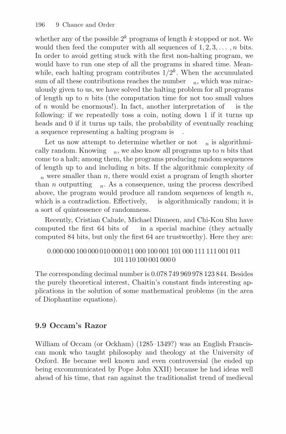
196 9 Chance and Order
whether any of the possible 2k programs of length k stopped or not. Wewould then feed the computer with all sequences of 1, 2, 3, . . . , n bits.In order to avoid getting stuck with the first non-halting program, wewould have to run one step of all the programs in shared time. Mean-while, each halting program contributes 1/2k. When the accumulatedsum of all these contributions reaches the number Ωn, which was mirac-ulously given to us, we have solved the halting problem for all programsof length up to n bits (the computation time for not too small valuesof n would be enormous!). In fact, another interpretation of Ω is thefollowing: if we repeatedly toss a coin, noting down 1 if it turns upheads and 0 if it turns up tails, the probability of eventually reachinga sequence representing a halting program is Ω.
Let us now attempt to determine whether or not Ωn is algorithmi-cally random. Knowing Ωn, we also know all programs up to n bits thatcome to a halt; among them, the programs producing random sequencesof length up to and including n bits. If the algorithmic complexity ofΩn were smaller than n, there would exist a program of length shorterthan n outputting Ωn. As a consequence, using the process describedabove, the program would produce all random sequences of length n,which is a contradiction. Effectively, Ω is algorithmically random; it isa sort of quintessence of randomness.
Recently, Cristian Calude, Michael Dinneen, and Chi-Kou Shu havecomputed the first 64 bits of Ω in a special machine (they actuallycomputed 84 bits, but only the first 64 are trustworthy). Here they are:
0.000 000 100 000 010 000 011 000 100 001 101 000 111 111 001 011101 110 100 001 000 0
The corresponding decimal number is 0.078 749 969 978 123 844. Besidesthe purely theoretical interest, Chaitin’s constant finds interesting ap-plications in the solution of some mathematical problems (in the areaof Diophantine equations).
9.9 Occam’s Razor
William of Occam (or Ockham) (1285–1349?) was an English Francis-can monk who taught philosophy and theology at the University ofOxford. He became well known and even controversial (he ended upbeing excommunicated by Pope John XXII) because he had ideas wellahead of his time, that ran against the traditionalist trend of medieval

9.9 Occam’s Razor 197
religious thought. Occam contributed to separating logic from meta-physics, paving the way toward an attitude of scientific explanation.A famous principle used by Occam in his works, known as the princi-ple of parsimony, principle of simplicity, or principle of economy, hasbeen raised to the level of an assessment/comparison criterion for thescientific reasonableness of contending theories. The principle is popu-larly known as Occam’s razor. It states the following: one should notincrease the number of explanatory assumptions for a hypothesis ortheory beyond what is absolutely necessary (unnecessary assumptionsshould be shaved off), or in a more compact form, the simpler the ex-planation, the better it is. When several competing theories are equal inother respects, the principle recommends selecting the theory that in-troduces the fewest assumptions and postulates the fewest hypotheticalentities.
The algorithmic complexity theory brings interesting support forOccam’s razor. In fact, a scientific theory capable of explaining a setof observations can be viewed as a minimal program reproducing theobservations and allowing the prediction of future observations. Letus then consider the probability P (s) of a randomly selected programproducing the sequence s. For that purpose and in analogy with thecomputation of Ω, each program outputting s contributes 1/2r to P (s),where r is the program length. It can be shown that P (s) = 1/2C(s),where C(s) represents the algorithmic complexity of s. Thus, sequenceswith low complexity occur more often than those with high complexity.If the assumptions required by a theorem are coded as sequences ofsymbols (for instance, as binary sequences), the most probable onesare the shortest.
Another argument stands out when considering the production ofbinary sequences of length n. If they are produced by a chance mecha-nism, they have probability 1/2n of showing up. Meanwhile, a possiblecause for the production of s could be the existence of another sequences∗ of length C(s) used as input in a certain machine. The probabilityof obtaining s∗ by random choice among all programs of length m is1/2C(s). The ratio 2−C(s)/2−n = 2n−C(s) thus measures the probabilitythat s occurred due to a definite cause rather than pure luck. Now, ifC(s) is much smaller than n, the probability that s occurred by pureluck is very small. One more reason to prefer simple theories!


10
Living with Chance
10.1 Learning, in Spite of Chance
Although immersed in a vast sea of chance, we have so far demon-strated that we are endowed with the necessary learning skills to solvethe problems arising in our daily life, including those whose solutionis a prerequisite to our survival as a species. Up to now, we have alsoshown that we are able to progress along the path of identifying thelaws (regularities) of nature. But it is not only the human species thatpossesses learning skills, i.e., the capability of detecting regularities inphenomena where chance is present. A large set of living beings alsomanifests the learning skills needed for survival. Ants, for instance,are able to determine the shortest path leading to some food source.The process unfolds as follows. Several ants leave their nest to foragefor food, following different paths; those that, by chance, reach a foodsource along the shortest path are sooner to reinforce that path withpheromones, because they are sooner to come back to the nest with thefood; those that subsequently go out foraging find a higher concentra-tion of pheromones on the shortest path, and therefore have a greatertendency (higher probability) to follow it, even if they did not followthat path before. There is therefore a random variation of the individualitineraries, but a learning mechanism is superimposed on that randomvariation – an increased probability of following the path with a higherlevel of pheromone –, which basically capitalizes on the law of largenumbers. This type of social learning, which we shall call sociogenetic,is common among insects.
Other classes of animals provide, not only examples of social learn-ing, but also individual learning, frequently depending on a schemeof punishment and reward. For instance, many animals learn to dis-

200 10 Living with Chance
tinguish certain food sources (leaves, fruits, nuts, etc.) according towhether they have a good taste (reward) or a bad taste (punishment).Human beings begin a complex learning process at a tender age, wheresocial and individual mechanisms complement and intertwine with eachother. Let us restrict the notion of learning here to the ability to clas-sify events/objects: short or long path, tasty or bitter fruit, etc. Thereare other manifestations of learning, such as the ability to assign valuesto events/objects or the ability to plan a future action on the basis ofprevious values of events/objects. However, in the last instance, thesemanifestations can be reduced to a classification: a fine-grained classi-fication (involving a large number of classes) in the case of assigningvalues to events/objects, or a fine-grained and extrapolated classifica-tion in the case of future planning.
Many processes of individual learning, which we shall call ontoge-netic, are similar to the guessing game mentioned in Chap. 9. Imaginea patient with suspicion of cardiovascular disease going to a cardiolo-gist. The event/object the cardiologist has to learn is the classificationof the patient in one of several diagnostic classes. This classificationdepends on the answer to several questions:
• Does the patient have a high cholesterol level?
• Is the patient overweight?
• Is the electrocardiogram normal?
• Does s(he) have cardiac arrhythmia?
We may call this type of learning, in which the learner is free to putwhatever questions s(he) wants, active learning . As seen in Chap. 9,active learning guarantees that the target object, in a possible domainof n objects (in the case of the cardiologist, n is the number of possiblediagnostic classes), is learned after presenting at most log2 n questions.(Of course things are not usually so easy in practice. At the start ofthe diagnostic process one does not have the answer to all possiblequestions and some of the available answers may be ambiguous.)
We may formalize the guessing game by assuming that one intendsto guess a number x belonging to the interval [0, 1], that some personX thought of. To guess the number, the reader L may randomly chosenumbers in [0, 1], following the guessing game strategy. Imagine thatthe number that X thought of is 0.3 and that the following sequenceof questions and answers takes place:

10.1 Learning, in Spite of Chance 201
L : Is it greater than 0.5?
X : No.
L : Is it greater than 0.25?
X : Yes.
And so on and so forth. After n questions, L comes to know x witha deviation that is guaranteed not to exceed 1/2n. Learning means hereclassifying x in one of the 2n intervals of [0, 1] with width 1/2n.
Things get more complicated when we are not free to present thequestions we want. Coming back to the cardiologist example, supposethat the consultation is done in a remote way and the cardiologist hasonly an abridged list of the ‘answers’. In this case the cardiologist isconstrained to learn the diagnosis using only the available data. Weare now dealing with a passive learning process. Is it also possible toguarantee learning in this case? The answer is negative. (As a matter offact, were the answer positive, we would probably already have learnedeverything there is to learn about the universe!)
Passive learning can be exemplified by learning the probability ofturning up heads in the coin-tossing game, when the results of n throwsare known. L is given a list of the results of n throws and L tries todetermine, on the basis of this list, the probability P of heads, a valuein [0, 1]. For this purpose L determines the frequency f of heads. Thelearning of P is obviously not guaranteed, in the sense that the bestone can obtain is a degree of certainty, for some tolerance of the de-viation between f and P . In passive learning there is therefore a newelement: there is no longer an absolute certainty of reaching a givendeviation between what we have learned and the ideal object/value tobe learned – as when choosing a number x in [0, 1]. Rather, we aredealing with degrees of certainty (confidence intervals) associated withthe deviations. When talking about Bernoulli’s law of large numbers inChap. 4, we saw how to establish a minimum value for n for probabilityestimation. The dotted line in Fig. 10.1 shows the minimum values of nwhen learning a probability, for several values of the deviation tolerancebetween f and P , and using a 95% certainty level.
Let us once again consider learning a number x in the interval [0, 1],but in a passive way this time. Let us assume that X has createda sequence of random numbers, all with the same distribution in [0, 1]and independent of each other, assigning a label or code according tothe numbers belonging (say, label 1) or not (say, label 0) to [0, x]. Thedistribution law for the random numbers is assumed unknown to L. To

202 10 Living with Chance
Fig. 10.1. Learning curvesshowing the minimum num-ber of cases (logarithmicscale) needed to learna probability (dotted curve)and a number (solid curve)with a given tolerance and95% certainty
fix ideas, suppose that X thought of x = 0.3 and L was given the list:
(0.37, 0) (0.29, 1) (0.63, 0) (0.13, 1) .
A list like this one, consisting of a set of labeled points (the objects inthis case), is known as a training set . On the basis of this training set,the best that L can do is to choose the value 0.29, with a deviation of0.01. Now suppose that the random numbers were such that L receivedthe list:
(0.78, 0) (0.92, 0) (0.83, 0) (0.87, 0) .
The best that L can do now is to choose 0.78, with a deviation of 0.48.In general, assuming that the distribution of the random numbers gen-erated by X is uniform, there is a 1/2n probability that all numbers fallin [0.5, 1]. If x < 0.5, the supplied list does not help L to learn a num-ber. In the worst case we may get a deviation of 0.5 with probabilityat least 1/2n.
It can be shown that in this learning of number x, in order to geta tolerance interval with 95% certainty, we need more cases than whenlearning the probability value in the coin-tossing experiment. The min-imum values of n in the passive learning of a number, for several val-ues of the deviation tolerance and using 95% certainty, are shown bythe solid curve in Fig. 10.1. Here is a concrete example: in order tolearn a probability with 0.1 tolerance and 95% certainty, 185 cases areenough. To learn a number under the same conditions requires at least1 696 trials. Learning a number when the probability law of the trainingset is unknown is more difficult than learning a probability. It requireslarger training sets in order to be protected against atypical trainingsets (for instance, all points in [0.5, 1]).
Finally, there is a third type of learning which we shall call phylo-genetic. It corresponds to the mechanisms of natural selection of the

10.1 Learning, in Spite of Chance 203
species, which grants a higher success to certain genomes to the detri-ment of others. Learning works as follows here: several gene combina-tions are generated inside the same species or phylum, via mutationsand hereditary laws. As a consequence, a non-homogeneous populationof individuals becomes available where a genomic variability compo-nent is present, as well as the individual traits that reflect it. Someindividuals are better off than others in the prosecution of certain vi-tal goals, tending therefore to a better success in genomic transmissionto the following generation. Thus, learning corresponds here to betterperformance in the face of the external environment.
In all these learning models, chance phenomena are present and, inthe last instance, it is the laws of large numbers that make learningpossible. In the simplest sociogenetic learning model, we have a homo-geneous set of individuals, each of them performing a distinct randomexperiment. Everything happens as if several individuals were throw-ing coins, with the throws performed under the same conditions. Herelearning resembles the convergence of an ‘ensemble average’. The moreindividuals there are, the better the learning will be.
In ontogenetic learning, we have a single individual carrying out orbeing confronted with random experiments as time goes by. This is thecase of ‘temporal average’ convergence that we have spoken about sooften. The more experiments there are, the better the learning will be.
In phylogenetic learning, the individuals are heterogeneous. We mayestablish an analogy with the coin-tossing case by assuming a living be-ing, called a ‘coin’, whose best performance given the external environ-ment corresponds to fairness: P (heads) = 1/2. At some instant there isa ‘coin’ population with different genes to which correspond differentvalues of P (heads). In the next generation, the ‘coins’ departing fromfairness get a non-null probability of being eliminated from the popula-tion, and with higher probability the more they deviate from fairness.Thus, in the following generation the distribution of P (heads) is dif-ferent from the one existing in the previous generation. We thus havea temporal convergence of the average resembling the one in Sect. 6.4.Meanwhile, the decision about which ‘coins’ to eliminate from eachgeneration depends on the departure of P (heads) from the better per-formance objective (fairness); that is, it depends on ‘ensemble average’convergence.
These different learning schemes are currently being used to buildso-called intelligent systems. Examples are ant colony optimization al-gorithms for sociogenetic learning, genetic algorithms for phylogeneticlearning, and artificial neural networks for ontogenetic learning.

204 10 Living with Chance
10.2 Learning Rules
In the preceding examples, learning consisted in getting close to a spec-ified goal (class label), close enough with a given degree of certainty,after n experiments, that is, for a training set having n cases. Thisnotion of learning is intimately related to the Bernoulli law of largenumbers and entirely in accordance with common sense. When a physi-cian needs to establish a diagnosis on the basis of a list of observations,s(he) uses a specific rule (or set of rules) with which s(he) expects toget close to the exact diagnosis with a given degree of certainty. Thisrule tries to value or weight the observations in such a way as to getclose to an exact diagnosis – which may be, for instance, having ornot having some disease – with a degree of certainty that increaseswith the number of diagnoses performed (the physician’s training set).The observations gathered in n clinical consultations and the evidenceobtained afterwards about whether the patient really had some dis-ease constitute the physician’s training set. As another example, whenlearning how to pronounce a word, say in French, by pronouncing it ntimes and receiving the comments of a French teacher, we expect to getclose to the correct pronunciation, with a given degree of certainty, asn increases. For that purpose, we use some rule (or set of rules) for ad-justing the pronunciation to ensure the above-mentioned convergence,in probability, to the correct pronunciation.
In all examples of task learning, there is the possibility of applyingone rule to the same observations (supposedly a learning rule), chosenfrom several possible rules. Let us go back to the problem of deter-mining a number x in [0, 1], in order to illustrate this aspect. We mayestablish a practical correspondence for this problem. For instance, thepractical task of determining the point of contact of two undergroundstructures (or rocks) on the basis of drilling results along some straightline. The drillings are assumed to be made at random points and withuniform distribution in some interval, as illustrated in Fig. 10.2. Theyreveal whether, at the drilling point, we are above structure 1 or abovestructure 2. If we are able to devise a rule behaving like the Bernoullilaw of large numbers in the determination of the contact point, we saythat the rule is a learning rule for the task at hand.
There are several feasible rules that can serve as learning rules forthis task. Let d be the estimate of the unknown contact point ∆ sup-plied by the rule. If the rule is d = xM, that is, select the maximumpoint (revealed as being) from structure 1 (rule 1), or d = xm, selectthe minimum point from structure 2 (rule 2), or again d = (xM+xm)/2

10.2 Learning Rules 205
Fig. 10.2. Drillings in some interval, designated by [0, 1], aiming to determinethe contact point ∆ between structure 1 (open circles) and structure 2 (solidcircles)
(rule 3), the rule is a learning rule, as illustrated in Fig. 10.3. The threerules produce a value d converging in probability (Bernoulli law of largenumbers) to ∆.
We now consider another version of the problem of finding a pointon a line segment. In contrast to what we had in the above problem,where there was a separation between the two categories of points, wenow suppose that this separation does not exist. Let us concretize thisscenario by considering a clinical analysis for detecting the presenceor absence of some disease. Our intention is to determine which value,produced by the analysis, separates the two classes of cases: the nega-tive ones (without disease) and the positive ones (with disease), whichwe denote N and P, respectively. Usually, clinical analyses do not al-low a total class separation, and instead one observes an overlap of therespective probabilistic distributions. Figure 10.4 shows an example ofthis situation.
In Fig. 10.4 we assume equal-variance normal distributions for thetwo classes of diagnosis. Whatever the threshold value d we may chooseon the straight line, we will always have to cope with a non-null clas-
Fig. 10.3. Average deviation d − ∆ curves (solid lines) with ±1 standarddeviation bounds (dotted lines), depending on the training set size n, com-puted in 25 simulations for ∆ = 0.5 and two learning rules: (a) d = xM, (b)d = (xM + xm)/2

206 10 Living with Chance
Fig. 10.4. Upper : Probability densities of a clinical analysis value for twoclasses, N and P. Lower : Possible training set
sification error. In the case of Fig. 10.4, the best value for d – the oneyielding a minimum error – is the one indicated in the figure (as sug-gested by the symmetry of the problem): d = ∆. The wrongly classifiedcases are the positive ones producing analysis values below ∆ and thenegative ones producing values above ∆. Unfortunately, in many prac-tical problems where one is required to learn the task ‘what is the best dseparating positive from negative cases?’, the probability distributionsare unknown. We are only given a training set like the one representedat the bottom of Fig. 10.4. What is then the behavior of the previousrules 1, 2 and 3? Rules 1 and 2 for infinite tailed distributions as inFig. 10.4 converge to values that are clearly far away from ∆, and hencethey do not behave as learning rules in this case. In fact, in this casewe will get a non-null probability of obtaining d values arbitrarily farfrom ∆. As for rule 3, it is still a learning rule for symmetrical distribu-tions, since it will lead on average and for the wrongly classified casesto a balance between positive and negative deviations from ∆. Had wewritten rule 3 as d = (xM + xm)/3, that is, changing the weight of therule parameters (xM, xm) from (1/2, 1/2) to (1/3, 2/3), the rule wouldno longer be a learning rule. In fact, even with parameters (1/2, 1/2),rule 3 is not, in general, a learning rule.
There are, however, more sophisticated rules that behave as learningrules for large classes of problems and distributions. One such rule isbased on a technique that reaches back to Abraham de Moivre. Itconsists in adjusting d so as to minimize the sum of squares of thedeviations for the wrongly classified cases. Another rule is based on thenotion of entropy presented in the last chapter. It consists in adjusting dso as to minimize the entropy of the classification errors and, therefore,their degree of disorder around the null error. (For certain classes ofproblems, my research team has shown that, surprisingly enough, itmay be preferable to maximize instead of minimizing the error entropy.)

10.3 Impossible Learning 207
10.3 Impossible Learning
As strange as it may look at first sight, there exist scenarios wherelearning is impossible. Some have to do with the distribution of thedata; others correspond to stranger scenarios. Let us first take a lookat an example of impossible learning for certain data distributions. Letus again consider the previous example of finding out a threshold value∆ separating two classes, N and P. The only difference is that we nowuse the following rule 4: we determine the averages of the values forclasses N and P, say mN and mP, and thereafter their average, that is,
d =mN + mP
2.
This is a learning rule for a large class of distributions, given the con-vergence in probability of averages. But we now consider the situa-tion where the distributions in both classes are Cauchy. As we saw inChap. 6, the law of large numbers is not applicable to Cauchy distri-butions, and the convergence in probability of averages does not holdin this case. The situation we will encounter is the one illustrated inFig. 10.5. Learning is impossible.
There are other and stranger scenarios where learning is impossible.Let us examine an example which has to do with expressing numbers ofthe interval [0, 1] in binary, as we did in the section on Borel’s normalnumbers in Chap. 6 and illustrated in Fig. 6.9. Let us assume thatX chooses an integer n that L has to guess using active learning. Ldoes not know any rule that might lead X to favor some integers overothers. For L everything happens as if X’s choice were made completelyat random. Since the aim is to learn/guess n, the game stipulates that
Fig. 10.5. The applicationof rule 4, under the sameconditions as in Fig. 10.3,for two classes with Cauchydistributed values

208 10 Living with Chance
L should ask X if a certain number in the interval [0, 1] contains thebinary digit dn. For instance, the number 0.3 represented in binary by0.01001100110011 . . . (repetition of 0011) does not contain d3, 0.001,which corresponds in decimal to 0.125. Here is an example of questionsand answers when X chooses n = 3 (d3):
L : 0.1?
X : 0 [(the binary representation of) 0.1 does not contain (thebinary representation of) 0.125].
L : 0.2?
X : 1 (0.2 contains 0.125).
L : 0.3?
X : 0 (0.3 does not contain 0.125).
L : 0.22?
X : 1 (0.22 contains 0.125).
The question now is: will L be able to guess n after a finite number ofquestions?
We first note that whatever di the learner L decides to present asa guess, s(he) always has 50% probability of hitting upon the valuechosen by X. This is due to the fact that, for a uniformly distributed xin [0, 1], the average of the di values for any selected value of x convergesto 0.5 independently of the chosen di. In other words, any random choicemade by L has always 50% probability of a hit. Is it possible that, byusing a sufficiently ‘clever’ rule, we will be able to substantially improveover this 50% probability? The surprising aspect comes now. Considerthe average of the absolute differences between what is produced by therule and what is produced by the right choice. In the above example,the values produced by the right choice 0.3 correspond to the 0101sequence of answers. Supposing that L, using some rule, decided 0.25,that is d2, we would get the 0010 sequence. The average of the absolutedifferences between what is produced by the rule and what is producedby the right choice is (0 + 1 + 1 + 1)/4 = 0.75. Now, this value alwaysconverges to 0.5 with an increasing number of questions because thedifference between any pair (dn, di) encloses a 0.5 area (as the readermay check geometrically). We may conclude that either L makes a hit,and the error is then zero, or s(he) does not make a hit, and the erroris then still 50%. There is no middle term in the learning process, ashappens in a vast number of scenarios, including the previous examples.Is it at least possible to arrive at a sophisticated rule allowing us to

10.4 To Learn Is to Generalize 209
reach the right solution in a finite number of steps? The answer isnegative. It is impossible to learn n from questions about the di set.
10.4 To Learn Is to Generalize
Let us look back at the example in Fig. 10.4. In a previous sectionwe were interested in obtaining a learning rule that would determinea separation threshold with minimum classification error. That is, weare making the assumption that the best type of classifier for the twoclasses (N and P) is a point. If we use rule 3, we may summarize thelearning task in the following way:
• Task to be learned: classify the value of a single variable (e.g., clinicalanalysis) in one of two classes.
• Classifier type: a number (threshold) x.
• Learning rule: rule 3.
This is a deductive approach to the classification problem. Once thetype of classifier has been decided, as well as the weighting of its pa-rameters, we apply the classifier in order to classify/explain new facts.We progress from the general (classifier type) to the particular (ex-plaining the observations). What can provide us with the guaranteethat the surmised classifier type is acceptable? It could well happenthat the diagnostic classes were ‘nested’, as shown in Fig. 10.6. In thecase of Fig. 10.6a, if we knew the class configuration, instead of consid-ering one threshold we would consider three and the classifier would be:If x is below d1 or between d2 and d3, it belongs to class N; otherwise,it belongs to class P. In the case of Fig. 10.6b, we would consider fivethresholds and the following classifier: If x is below d1 or between d2
and d3, or between d4 and d5, then x belongs to class N ; otherwise,it belongs to class P. Classifiers involving one, three or five thresholdsare linear in the respective parameters. In other scenarios it could wellhappen that the most appropriate classifier is quadratic, as in Fig. 10.7,where we separate the two classes with: If x2 is greater than d, then xbelongs to class N ; otherwise, it belongs to class P. We may go on imag-ining the need to use ever more complex types of classifier, in particularwhen a larger number of parameters is involved.
Meanwhile, we never know, in general, if we are confronted withthe configuration of Figs. 10.6a, 10.6b, 10.7, or some other situation.All we usually have available are simply the observations constituting

210 10 Living with Chance
Fig. 10.6. Situation of classes N(white) and P (grey) separatedby three (a) and five (b) thresh-olds. The training set is the sameas in Fig. 10.4
Fig. 10.7. Quadratic classifier
our training set. How can we then choose which type of classifier touse? In this situation we intend to determine the classifier type andits parameters simply on the basis of the observations, without anyassumptions, or with only a minimum of assumptions. Learning is nowinductive. We progress from the particular (the observations) to thegeneral (classifier type). The answer to the question of what type ofclassifier to use is related to the difficult generalization capability issueof inductive learning .
Suppose from now on that in the above example the distributions ofthe analysis value x for the two classes of diagnosis did correspond, infact, to the four-structure situation of Fig. 10.6a. However, the personwho designed the classifier does not know this fact; s(he) only knowsthe training set. The classification rule based on three thresholds is thenadequate. The only thing we have to do is to use a learning rule forthis type of classifier, which adjusts the three thresholds to the threeunknown values ∆1, ∆2, and ∆3, in order to minimize the number oferrors. Let us further suppose that in the case of Fig. 10.6a we werefortunate with the training set supplied to us and we succeeded indetermining d1, d2, and d3 quite close to the true thresholds ∆1, ∆2,and ∆3. Our solution would then behave equally well, on average terms,for other (new) sets of values, affording the smallest probability of error.The designed classifier would allow generalization and would generalizewell (with the smallest probability of error, on average). We could havebeen unfortunate, having to deal with an atypical training set, leadingto the determination of d1, d2, and d3 far away from the true values. Inthis case, the classifier designed on the basis of the training set wouldnot generalize to our satisfaction.
In summary, we can never be certain that a given type of classifierallows generalization. The best we can have is some degree of certainty.But what does this degree of certainty depend on? In fact, it depends

10.5 The Learning of Science 211
on two things: the number of elements of the training set and the com-plexity of the classifier (number of parameters and type of classifier).As far as the number of training set elements is concerned, it is easilyunderstandable that, as we increase that number, the probability of thetraining set being typical also increases, in the sense of the strong lawof large numbers mentioned in Chap. 6.
Let us now focus on the complexity issue. In the present examplethe complexity has to do with the number of thresholds used by theclassifier. The simpler the classifier, the easier the generalization. Forthe above example, the classifier with a single threshold does not needsuch large training sets as the three-threshold classifier, in order togeneralize; however, its generalization is always accompanied by a non-null classification error. It generalizes, but does so rather poorly. Weare thus in a sub-learning situation. At the other extreme, the five-threshold classifier does not generalize in any reasonable way, since itsperformance behaves erratically; in training sets like those of Fig. 10.6,it attains zero errors, whereas in new data sets it may produce veryhigh error rates. We are thus in an over-learning situation, where theclassifier, given its higher complexity, gets so stuck to the training setdetails that it will not behave in a similar way when applied to other(new) data sets. We may say that the one-threshold classifier only de-scribes the coarse-grained structure of the training set, while the five-threshold classifier describes a structure that is too finely grained, verymuch influenced by the random idiosyncrasies of the training set. Thethree-threshold classifier is the best compromise solution for the learn-ing task. Finding such a best compromise is not always an easy task inpractice.
10.5 The Learning of Science
Occam’s razor told us that, in the presence of uncertainty, the simplestexplanations are the best. Consider the intelligibility of the universe,or in other words the scientific understanding of material phenomena.If, in order to explain a given set of observations of these phenomena,say n observations, we needed to resort to a rule using n parameters,we could say that no intelligibility was present. There is no differencebetween knowing the rule and knowing the observations. In fact, tounderstand is to compress. The intelligibility of the universe exists onlyif infinitely many observations can be explained by laws with a reducednumber of parameters. It amounts to having a small program that
212 10 Living with Chance
is able to produce infinitely many outcomes. This is the aim of the‘theory of everything’ that physicists are searching for, encouraged bythe appreciation that, up to now, simple, low complexity (in the abovesense) laws have been found that are capable of explaining a multitudeof observations. We will never be certain (fortunately!) of having foundthe theory of everything. On the other hand, inductively learning thelaws of the universe – that is, obtaining laws based on observationsalone –, presents the problem of their generalization: can we be certain,with a given level of certainty, that the laws we have found behaveequally well for as yet unobserved cases?
The Russian mathematician Vladimir Vapnik developed pioneeringwork in statistical learning theory, establishing (in 1991) a set of theo-retical results which allow one in principle to determine a degree of cer-tainty with which a given classifier (or predictive system) generalizes.Statistical learning theory clarifies what is involved in the inductivelearning model, supplying an objective foundation for inductive valid-ity. According to this theory we may say that the objective foundationof inductive validity can be stated in a compact way as follows: in orderto have an acceptable degree of certainty about the generalization ofour inductive model (e.g., classifier type), one must never use a morecomplex type of model than is allowed by the available data. Now,one of the interesting aspects of the theory developed by Vapnik isthe characterization of the generalizing capability by means of a singlenumber, known as the Vapnik–Chervonenkis dimension (often denotedby DVC). A learning model can only be generalized if its DVC is finite,and all the more easily as its value is smaller. There are certain modelswith infinite DVC. The parameters of such models can be learned sothat a complete separation of the values of any training set into therespective classes can be achieved, no matter how complex those valuesare and even if we deliberately add incorrect class-labeled values to thetraining set.
The fact that an inductive model must have finite DVC in orderto be valid and therefore be generalizable is related to the falsifiabilitycriterion proposed by the Austrian philosopher Karl Popper for demar-cating a theory as scientific. As a matter of fact, in the same way asclassifiers with infinite DVC will never produce incorrect classificationson any training set (even if deliberately incorrectly labeled observa-tions are added), it can be said that non-scientific theories will nevererr; they always explain the observations, no matter how strange theyare. On the other hand, if scientific laws are used – thus, capable ofgeneralization –, we are in a situation corresponding to the use of finite
10.6 Chance and Determinism: A Never-Ending Story 213
DVC classifiers; that is, it is possible to present observational data thatis not explainable by the theory (falsifying the theory).
Occam’s razor taught us to be parsimonious in the choice of thenumber of parameters of the classifier (more generally, of the learningsystem). Vapnik’s theory goes a step further. It tells us the level ofcomplexity of the classifier (or learning system) to which we may gofor a certain finite number of observations, in such a way that learningwith generalization is achievable.
10.6 Chance and Determinism: A Never-Ending Story
It seems that God does play dice after all, contradicting Albert Ein-stein’s famous statement. It seems that the decision of where a photongoes or when a beta emission takes place is of divine random origin, as isthe knowledge of the infinitely many algorithmically complex numbers,readily available to create a chaotic phenomenon.
The vast majority of the scientific community presently supports thevision of a universe where chance events of objective nature do exist. Wehave seen that it was not always so. Suffice it to remember the famousstatement by Laplace, quoted in Chap. 7. There is, however, a minorityof scientists who defend the idea of a computable universe. This idea– perhaps better referred to as a belief, because those that advocate itrecognize that it is largely speculative, and not supported by demon-strable facts – is mainly based on some results of computer science: thecomputing capacity of the so-called cellular automata and the algorith-mic compression of information. Cellular automata are somewhat liketwo- and three-dimensional versions of the quadratic iterator presentedin Chap. 7, in the sense that, by using a set of simple rules, they cangive rise to very complex structures, which may be used as models ofsuch complex phenomena as biological growth. Algorithmic compres-sion of information deals with the possibility of a simple program beingable to generate a sequence that passes all irregularity tests, like thosementioned in Chap. 9 concerning the digit sequences of π, e and
√2.
On the basis of these ideas, it has been proposed that everything in theuniverse is computable, with these proposals ranging from an extremevision of a virtual reality universe – a universe without matter, somesort of hologram –, to a less extreme vision of an inanimate universebehaving as if it were a huge computer.
There are of course many relevant and even obvious objectionsto such visions of a computable universe [42]. The strongest objec-

214 10 Living with Chance
Fig. 10.8. Whenfurther observationsare required
tion to this neo-deterministic resurrection has to do with the non-computability of pure chance, i.e., of quantum randomness. The mostprofound question regarding the intelligibility of the universe thus askswhether it is completely ordered or chaotic; in other words, whetherchance is a deterministic product of nature or one of its fundamentalfeatures. If the universe has infinite complexity, as believed by the ma-jority of scientists, it will never be completely understood. Further, wedo not know whether the complexity of a living being can be explainedby a simple program. We do not know, for instance, which rules in-fluence biological evolution, in such a way that we may forecast whichpath it will follow. Are mutations a phenomenon of pure chance? Wedo not know. Life seems to be characterized by an infinite complexitywhich we will never be able to learn in its entirety.
As a matter of fact, as we said already in the preface, if there wereno chance events, the temporal cause–effect sequences would be de-terministic and, therefore, computable, although we might need hugeamounts of information for that purpose. It remains to be seen whetherone would ever be able to compute those vast quantities of informationin a useful time. Notwithstanding, the profound conviction of the scien-tific community at present is that objective chance is here to stay. Wemay nevertheless be sure of one thing – really sure with a high degree ofcertainty – that chance and determinism will forever remain a subjectof debate, since objective chance will always remain absolutely beyondthe cognition of human understanding.

A
Some Mathematical Notes
A.1 Powers
For integer n (i.e., a whole number, without fractional part), the ex-pression xn, read x to the power n, designates the result of multiplyingx by itself n times. x is called the base and n the exponent . If n ispositive, the calculation of xn is straightforward, e.g.,
2.53 = 2.5 × 2.5 × 2.5 = 15.625 .
From the definition, one has
xn × xm = xn+m , (xn)m = xnm ,
where nm means n × m, e.g.,
2.55 = 2.53 × 2.52 = 2.5 × 2.5 × 2.5 × 2.5 × 2.5 = 97.65625 ,
(0.52)3 = (0.5)6 = 0.015 625 .
In the book, expressions such as (2/3)6 sometimes occur. We may applythe definition directly, as before, or perform the calculation as
(2/3)6 = 26/36 = 64/729 .
Note also that 1n is 1.
From xn × xm = xn+m comes the convention x0 = 1 (for any x).Moreover, for a negative exponent, −n, we have
x−n =1
xn,

216 A Some Mathematical Notes
since
xn × x−n = x0 = 1 .
For example,
2−3 =1
23=
1
8.
Powers with fractions as exponents and non-negative bases are calcu-lated as a generalization of (xn)m = xnm. For instance, from (x1/2)2 =x, one has x1/2 =
√x .
A.2 Exponential Function
The figure below shows the graphs of functions y = x4 and y = 2x.Both are calculated with the above power rules. In the first function,the exponent is constant; the function is a power function. In the secondfunction the base is constant; it is an exponential function. Figure A.1shows the fast growth of the exponential function in comparison withthe power function. Given any power and exponential functions, it isalways possible to find a value x beyond which the exponential is abovethe power.
Given an exponential function ax, its growth rate (measured by theslope at each point of the curve) is given by Cax, where C is a constant.C can be shown to be 1 when a is the value to which (1 + 1/h)h tendswhen the integer h increases arbitrarily. Let us see some values of thisquantity:
(
1 +1
2
)2
= 1.52 = 2.25 ,
Fig. A.1. Comparing the growthof the exponential function andthe power function

A.3 Logarithm Function 217
(
1 +1
10
)10
= 1.110 = 2.593 742 ,
(
1 +1
1000
)1000
= 1.0011000 = 2.716 924 2 .
These quantities converge to the natural or Napier number , denotedby e. The value of e to 6 significant figures is 2.718 28. The naturalexponential ex thus enjoys the property that its growth rate is equal toitself.
A.3 Logarithm Function
The logarithm function is the inverse of the exponential function; thatis, given y = ax, the logarithm of y in base a is x. The word ‘log-arithm’, like the word ‘algorithm’, comes from Khwarizm, presentlyKhiva in Uzbekistan, birth town of Abu Ja’far Muhammad ibn MusaAl-Khwarizmi (780–850), author of the first treatise on algebra.
This function is usually denoted by loga. Here are some examples:
• log2(2.25) = 1.5, because 1.52 = 2.25.
• log10(2.593 742) = 1.1, because 1.110 = 2.593 742.
• loga(1) = 0, because as we have seen, a0 = 1 for any a.
The logarithm function in the natural base, viz., loge(x), or simplylog(x), is frequently used. An important property of log(x) is that itsgrowth rate is 1/x. The graphs of these functions are shown in Fig. A.2.
Fig. A.2. The logarithm function

218 A Some Mathematical Notes
Fig. A.3. The behavior of thefunctions log(x4) and log(2x)
The following results are a consequence of the properties of thepower function:
log(xy) = log(x) + log(y) , log(xy) = y log(x) .
The logarithm function provides a useful transformation in the analysisof fast growth phenomena. For instance, in Fig. A.1 it is not possibleto compare the growth of the two functions for very small or very highvalues of x. If we apply the log transformation, we get
log(x4) = 4 log(x) , log(2x) = x log(2) ,
whose graphs are shown in Fig. A.3. The behavior of the two functionsis now graphically comparable. It becomes clearly understandable that,in the long run, any exponential function overtakes any power function.
A.4 Factorial Function
The factorial function of a positive integer number n, denoted n!, isdefined as the product of all integers from n down to 1:
n! = n × (n − 1) × (n − 2) × . . . × 2 × 1 .
The factorial function is a very fast-growing function, as can be checkedin the graphs of Fig. A.4. In the left-hand graph, n! is represented to-gether with x4 and 2x, while the respective logarithms are shown on theright. In the long run, the factorial function overtakes any exponentialfunction.

A.5 Sinusoids 219
Fig. A.4. Left : The functions n!, x4 and 2x. Right : Logarithms of the threefunctions on the left
A.5 Sinusoids
The sine function sin(x) (sine of x) is defined by considering the radiusOP of a unit-radius circle enclosing the angle x, measured in the an-ticlockwise direction in Fig. A.5. The function represents the length ofthe segment AP drawn perpendicularly from P to the horizontal axis.
The length can be either positive or negative, depending on whetherthe segment is above or below the horizontal axis, respectively. Withthe angle measured in radians, that is, as an arc length represented bya certain fraction of the unitary radius, and since 2π is the circumfer-ence, one has
sin(0) = sin(π) = sin(2π) = 0 , sin(π/2) = 1 ,
sin(3π/2) = −1 , sin(π/4) =√
2/2 .
The inverse function of sin(x) is arcsin(x) (arcsine of x). As an example,arcsin(
√2/2) = π/4 (for an arc between 0 and 2π).
Considering point P rotating uniformly around O, so that it de-scribes a whole circle every T seconds, the segment AP will varyas sin(2πt/T ), where t is the time, or equivalently sin(2πft), wheref = 1/T is the frequency (cycles per second). If the movement of Pstarts at the position corresponding to the angle φ, called the phase,the segment will vary as sin(2πft + φ) (see Fig. 8.8).
The cosine function cos(x) (cosine of x) corresponds to the segmentOA in Fig. A.5. Thus,
cos(0) = cos(2π) = 1 , cos(π) = −1 ,
cos(π/2) = cos(3π/2) = 0 , cos(π/4) =√
2/2 .

220 A Some Mathematical Notes
Fig. A.5. Unit circle and definition of the sine andcosine functions
From Pythagoras’ theorem, one always has
sin2(x) + cos2(x) = 1 ,
for any x.
A.6 Binary Number System
In the decimal system which we are all accustomed to, the value ofany number is obtained from the given representation by multiplyingeach digit by the corresponding power of ten. For instance, the digitsequence 375 represents
3 × 10² + 7 × 101 + 5 × 100 = 300 + 70 + 5 .
The rule is the same when the number is represented in the binarysystem (or any other system base for that matter). In the binary systemthere are only two digits (commonly called bits): 0 and 1. Here are someexamples: 101 has value
1 × 22 + 0 × 21 + 1 × 20 = 4 + 1 = 5 ,
while 0.101 has value
1 × 2−1 + 0 × 2−2 + 1 × 2−3 = 1/2 + 1/8 = 0.5 + 0.125 = 0.625 .

References
The following list of references includes works of popular science and othersources that are not not technically demanding.
1. Alvarez, L.: A pseudo-experience in parapsychology (letter), Science 148,1541 (1965)
2. Amaral, L., Goldberger, A., Ivanov, P., Stanley, E.: Modeling heart ratevariability by stochastic feedback, Comp. Phys. Communications 121–2,126–128 (1999)
3. Ambegaokar, V.: Reasoning about Luck. Probability and Its Uses inPhysics , Cambridge University Press (1996)
4. Bar-Hillel, M., Wagenaar, W.A.: The perception of randomness, Advancesin Applied Mathematics 12, 428–454 (1991)
5. Bassingthwaighte, J.B., Liebovitch, L., West, B.: Fractal Physiology, Ox-ford University Press (1994)
6. Beltrami, E.: What is Random? , Springer-Verlag (1999)
7. Bennet, D.J.: Randomness , Harvard University Press (1998)
8. Bernstein, P.: Against the Gods. The Remarkable Story of Risk , JohnWiley & Sons (1996)
9. Blackmore, S.: The lure of the paranormal, New Scientist 22, 62–65 (1990)
10. Bolle, F.: The envelope paradox, the Siegel paradox, and the impossi-bility of random walks in equity and financial markets, www.econ.euv-frankfurto.de/veroeffentlichungen/bolle.html (2003)
11. Bouchaud, J.-P.: Les lois des grands nombres, La Recherche 26, 784–788(1995)
12. Brown, J.: Is the universe a computer? New Scientist 14, 37–39 (1990)

222 References
13. Casti, J.: Truly, madly, randomly, New Scientist 155, 32–35 (1997)
14. Chaitin, G.: Randomness and mathematical proof, Scientific American232, No. 5, 47–52 (1975)
15. Chaitin, G.: Randomness in arithmetic, Scientific American 259, No. 7,52–57 (1988)
16. Chaitin, G.: Le hasard des nombres, La Recherche 22, 610–615 (1991)
17. Chaitin, G.: L’Univers est-il intelligible? La Recherche 370, 34–41 (2003)
18. Crutchfield, J., Farmer, J.D., Packard, N., Shaw, R.: Chaos, ScientificAmerican 255, No. 6, 38–49 (1986)
19. Deheuvels, P.: La probabilite, le hasard et la certitude, collection Que Sais-Je?, Presses Universitaires de France (1982)
20. Devlin, K.: The two envelopes paradox. Devlin’s angle, MAA On-line, The Mathematical Association of America, www.maa.org/devlin/devlin 0708 04.html (2005)
21. Diaconis, P., Mosteller, F.: Methods for studying coincidences, Journal ofthe American Statistical Association 84, 853–861 (1989)
22. Droesbeke, J.-J., Tassi, P.: Histoire de la statistique, collection Que Sais-Je?, Presses Universitaires de France (1990)
23. Everitt, B.S.: Chance Rules. An Informal Guide to Probability, Risk andStatistics , Springer-Verlag (1999)
24. Feynman, R.: QED. The Strange Theory of Light and Matter , Penguin,London (1985)
25. Ford, J.: What is chaos that we should be mindful of? In: The NewPhysics , ed. by P. Davies, Cambridge University Press (1989)
26. Gamow, G., Stern, M.: Jeux Mathematiques. Quelques casse-tete, Dunod(1961)
27. Gell-Mann, M.: The Quark and the Jaguar , W.H. Freeman (1994)
28. Ghirardi, G.: Sneaking a Look at God’s Cards. Unraveling the Mysteriesof Quantum Mechanics, Princeton University Press (2005)
29. Gindikin, S.: Tales of Physicists and Mathematicians, Birkhauser, Boston(1988)
30. Goldberger, A., Rigney, D., West, B.: Chaos and fractals in human phys-iology, Scientific American 262, No. 2, 35–41 (1990)
31. Haken, H., Wunderlin, A.: Le chaos deterministe, La Recherche 21, 1248–1255 (1990)

References 223
32. Hanley, J.: Jumping to coincidences: Defying odds in the realm of thepreposterous, The American Statistician 46, 197–202 (1992)
33. Haroche, S., Raimond, J.-M., Brune, M.: Le chat de Schrodinger se pretea l’experience, La Recherche 301, 50–55 (1997)
34. Henon, M.: La diffusion chaotique, La Recherche 209, 490–498 (1989)
35. Idrac, J.: Mesure et instrument de mesure, Dunod (1960)
36. Jacquard, A.: Les Probabilites , collection Que Sais-Je?, Presses Universi-taires de France (1974)
37. Kac, M.: What is Random?, American Scientist 71, 405–406 (1983)
38. Layzer, D.: The arrow of time, Scientific American 233, No. 6, 56–69(1975)
39. Mandelbrot, B.: A multifractal walk down Wall Street, Scientific American280, No. 2, 50–53 (1999)
40. Martinoli, A., Theraulaz, G., Deneubourg, J.-L.: Quand les robots imitentla nature, La Recherche 358, 56–62 (2002)
41. McGrew, T.J., Shier, D., Silverstein, H.S.: The two-envelope paradox re-solved, Analysis 57.1, 28–33 (1997)
42. Mitchell, M.: L’Univers est-il un calculateur? Quelques raisons pourdouter, La Recherche 360, 38–43 (2003)
43. Nicolis, G.: Physics of far-from-equilibrium systems and self-organisation.In: The New Physics, ed. by P. Davies, Cambridge University Press (1989)
44. Ollivier, H., Pajot, P.: La decoherence, espoir du calcul quantique, LaRecherche 378, 34–37 (2004)
45. Orlean, A.: Les desordres boursiers, La Recherche 22, 668–672 (1991)
46. Paulson, R.: Using lottery games to illustrate statistical concepts andabuses, The American Statistician 46, 202–204 (1992)
47. Peitgen, H.-O., Jurgens, H., Saupe, D.: Chaos and Fractals. New Frontiersof Science, Springer-Verlag (2004)
48. Perakh, M.: Improbable probabilities, www.nctimes.net/~mark/bibl
science/probabilities.htm (1999)
49. Pierce, J.: An Introduction to Information Theory. Symbols, Signals andNoise, Dover Publications (1980)
50. Pincus, S.M.: Assessing serial irregularity and its implications for health,Proc. Natl. Acad. Sci. USA 954, 245–267 (2001)
51. Polkinghorne, J.C.: The Quantum World , Princeton University Press(1984)

224 References
52. Postel-Vinay, O.: L’Univers est-il un calculateur? Les nouveaux demi-urges, La Recherche 360, 33–37 (2003)
53. Rae, A.: Quantum Physics: Illusion or Reality? , 2nd edn., CambridgeUniversity Press (2004)
54. Rittaud, B.: L’Ordinateur a rude epreuve, La Recherche 381, 28–35 (2004)
55. Ruelle, D.: Hasard et chaos , collection Points, Editions Odile Jacob (1991)
56. Salsburg, D.: The Lady Tasting Tea: How Statistics Revolutionized Sciencein the Twentieth Century, W.H. Freeman (2001)
57. Schmidhuber, J.: A computer scientist’s view of life, the universe, andeverything, http://www.idsia.ch/~juergen/everything (1997)
58. Shimony, A.: Conceptual foundations of quantum mechanics. In: The NewPhysics , ed. by P. Davies, Cambridge University Press (1989)
59. Steyer, D.: The Strange World of Quantum Mechanics, Cambridge Uni-versity Press (2000)
60. Taylor, J.: An Introduction to Error Analysis, 2nd edn., University ScienceBooks (1997)
61. Tegmark, M., Wheeler, J.A.: 100 years of quantum mysteries, ScientificAmerican 284, 54–61 (2001)
62. UCI Machine Learning Repository (The Boston Housing Data): Websitewww.ics.uci.edu/~mlearn/MLSummary.html
63. West, B., Goldberger, A.: Physiology in fractal dimensions, American Sci-entist 75, 354–364 (1987)
64. West, B., Shlesinger, M.: The noise in natural phenomena, American Sci-entist 78, 40–45 (1990)
65. Wikipedia: Ordre de grandeur (nombre), fr.wikipedia.org/wiki/
Ordre de grandeur (nombre) (2005)