Ch 7.9: Nonhomogeneous Linear Systems

The general theory of a nonhomogeneous system of equations

parallels that of a single nth order linear equation.

This system can be written as x' = P(t)x + g(t), where

)()()()(

)()()()(

)()()()(

2211

222221212

112121111

tgxtpxtpxtpx

tgxtpxtpxtpx

tgxtpxtpxtpx

nnnnnnn

nn

nn

)()()(

)()()(

)()()(

)(,

)(

)(

)(

)(,

)(

)(

)(

)(

21

22221

11211

2

1

2

1

tptptp

tptptp

tptptp

t

tg

tg

tg

t

tx

tx

tx

t

nnnn

n

n

nn

Pgx

General Solution

The general solution of x' = P(t)x + g(t) on I: < t < has the form

where

is the general solution of the homogeneous system x' = P(t)x

and v(t) is a particular solution of the nonhomogeneous system x' = P(t)x + g(t).

)()()()( )()2(2

)1(1 ttctctc n

n vxxxx

)()()( )()2(2

)1(1 tctctc n

nxxx

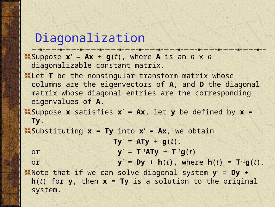
Diagonalization

Suppose x' = Ax + g(t), where A is an n x n diagonalizable constant matrix.

Let T be the nonsingular transform matrix whose columns are the eigenvectors of A, and D the diagonal matrix whose diagonal entries are the corresponding eigenvalues of A.

Suppose x satisfies x' = Ax, let y be defined by x = Ty.

Substituting x = Ty into x' = Ax, we obtain

Ty' = ATy + g(t).

or y' = T-1ATy + T-1g(t)

or y' = Dy + h(t), where h(t) = T-1g(t).

Note that if we can solve diagonal system y' = Dy + h(t) for y, then x = Ty is a solution to the original system.

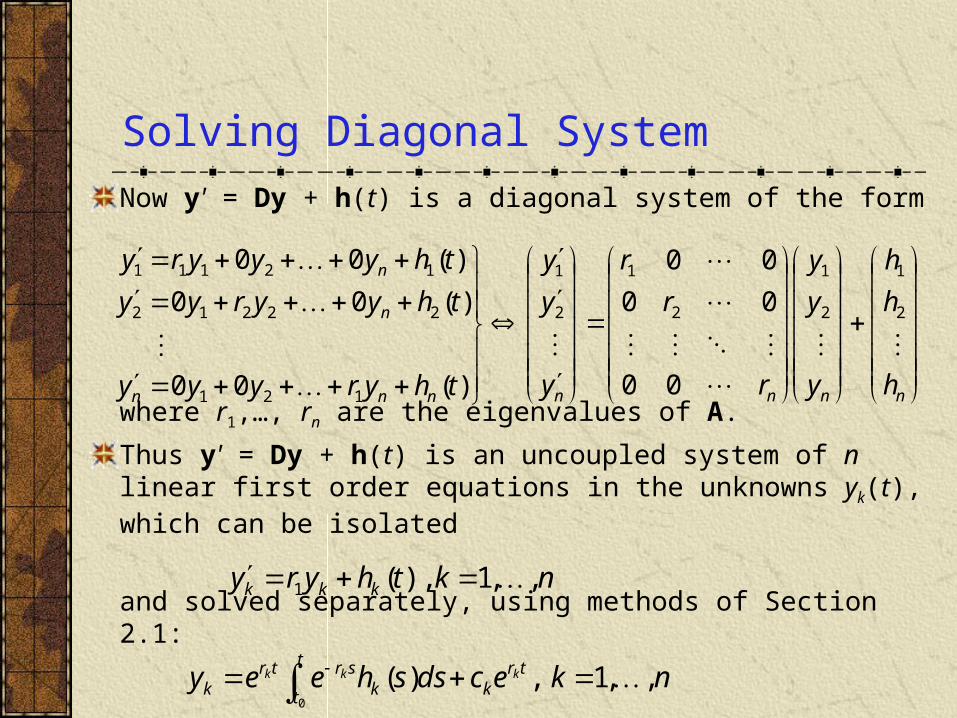
Solving Diagonal System

Now y' = Dy + h(t) is a diagonal system of the form

where r1,…, rn are the eigenvalues of A.

Thus y' = Dy + h(t) is an uncoupled system of n linear first order equations in the unknowns yk(t), which can be isolated

and solved separately, using methods of Section 2.1:

nnnnnnn

n

n

h

h

h

y

y

y

r

r

r

y

y

y

thyryyy

thyyryy

thyyyry

2

1

2

1

2

1

2

1

121

22212

12111

00

00

00

)(00

)(00

)(00

nkthyry kkk ,,1),(1

nkecdssheeyt

t

trkk

srtrk

kkk ,,1,)(0

Solving Original System

The solution y to y' = Dy + h(t) has components

For this solution vector y, the solution to the original system

x' = Ax + g(t) is then x = Ty.

Recall that T is the nonsingular transform matrix whose columns are the eigenvectors of A.

Thus, when multiplied by T, the second term on right side of yk produces general solution of homogeneous equation, while the integral term of yk produces a particular solution of nonhomogeneous system.

nkecdssheeyt

t

trkk

srtrk

kkk ,,1,)(0

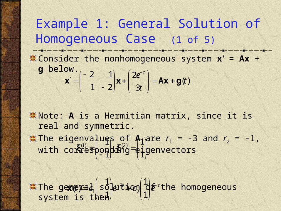
Example 1: General Solution of Homogeneous Case (1 of 5)

Consider the nonhomogeneous system x' = Ax + g below.

Note: A is a Hermitian matrix, since it is real and symmetric.

The eigenvalues of A are r1 = -3 and r2 = -1, with corresponding eigenvectors

The general solution of the homogeneous system is then

)(3

2

21

12t

t

e t

gAxxx

1

1,

1

1 )2()1( ξξ

tt ecect

1

1

1

1)( 2

31x

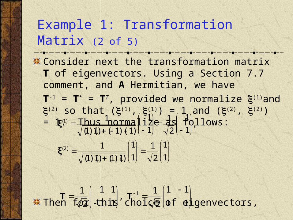
Example 1: Transformation Matrix (2 of 5)

Consider next the transformation matrix T of eigenvectors. Using a Section 7.7 comment, and A Hermitian, we have

T-1 = T* = TT, provided we normalize (1)and (2) so that ((1), (1)) = 1 and ((2), (2)) = 1. Thus normalize as follows:

Then for this choice of eigenvectors,

1

1

2

1

1

1

)1)(1()1)(1(

1

,1

1

2

1

1

1

)1)(1()1)(1(

1

)2(

)1(

ξ

ξ

11

11

2

1,

11

11

2

1 1TT

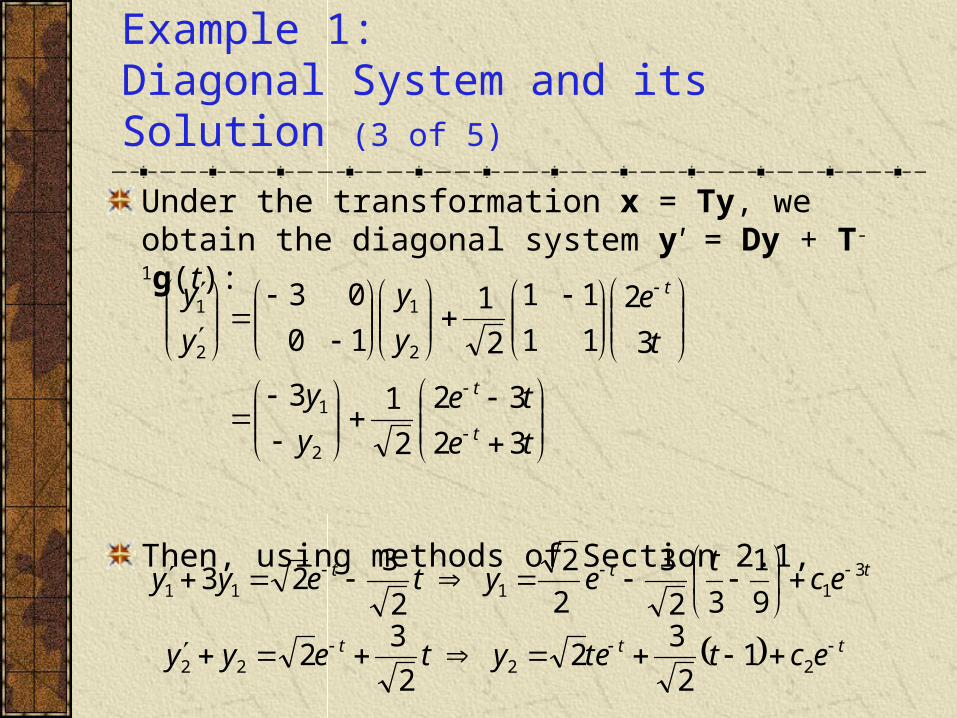
Example 1: Diagonal System and its Solution (3 of 5)

Under the transformation x = Ty, we obtain the diagonal system y' = Dy + T-1g(t):

Then, using methods of Section 2.1,

te

te

y

y

t

e

y

y

y

y

t

t

t

32

32

2

13

3

2

11

11

2

1

10

03

2

1

2

1

2

1

ttt

ttt

ectteyteyy

ect

eyteyy

2222

31111

12

32

2

32

9

1

32

3

2

2

2

323

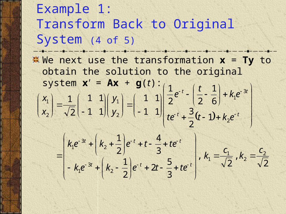
Example 1: Transform Back to Original System (4 of 5)

We next use the transformation x = Ty to obtain the solution to the original system x' = Ax + g(t):

2,

2,

3

52

2

13

4

2

1

12

36

1

22

1

11

11

11

11

2

1

22

11

23

1

23

1

2

31

2

1

2

1

ck

ck

tetekek

tetekek

ektte

ekt

e

y

y

x

x

ttt

ttt

tt

tt

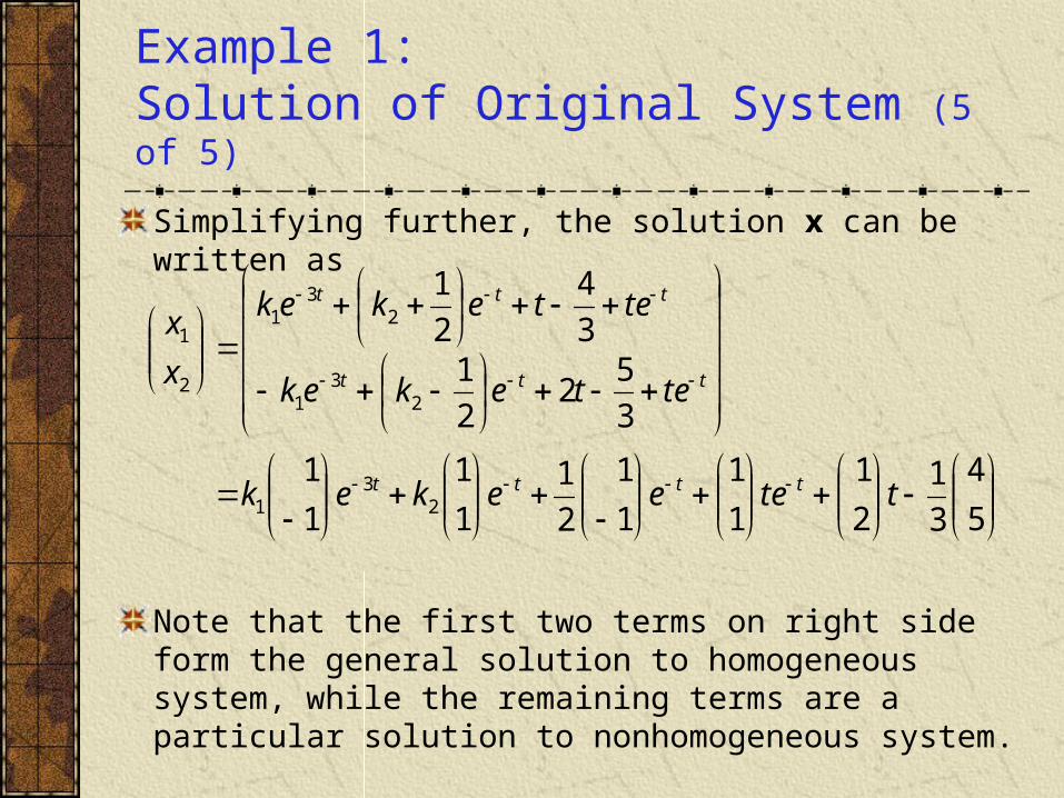
Example 1: Solution of Original System (5 of 5)

Simplifying further, the solution x can be written as

Note that the first two terms on right side form the general solution to homogeneous system, while the remaining terms are a particular solution to nonhomogeneous system.

5

4

3

1

2

1

1

1

1

1

2

1

1

1

1

1

3

52

2

13

4

2

1

23

1

23

1

23

1

2

1

tteeekek

tetekek

tetekek

x

x

tttt

ttt

ttt

Summary (1 of 2)

The method of undetermined coefficients requires no integration but is limited in scope and may involve several sets of algebraic equations.

Diagonalization requires finding inverse of transformation matrix and solving uncoupled first order linear equations. When coefficient matrix is Hermitian, the inverse of transformation matrix can be found without calculation, which is very helpful for large systems.

The Laplace transform method involves matrix inversion, matrix multiplication, and inverse transforms. This method is particularly useful for problems with discontinuous or impulsive forcing functions.

Summary (2 of 2)

Variation of parameters is the most general method, but it involves solving linear algebraic equations with variable coefficients, integration, and matrix multiplication, and hence may be the most computationally complicated method.

For many small systems with constant coefficients, all of these methods work well, and there may be little reason to select one over another.