CFD Analysis of Mixing Characteristics of Several Fuel ...€¦ · CFD Analysis of Mixing Characteristics of Several Fuel Injectors at Hypervelocity Flow Conditions. ... The shock

CFD Analysis of Mixing Characteristics of Several Fuel Injectors atHypervelocity Flow Conditions.

Tomasz G. Drozda,∗ J. Philip Drummond,† and Robert A. Baurle ‡

NASA Langley Research Center, Hampton, VA, 23681

CFD analysis is presented of the mixing characteristics and performance of three fuel injectorsat hypervelocity flow conditions. The calculations were carried out using the VULCAN-CFD solverand Reynolds-Averaged Simulations (RAS). The high Mach number flow conditions match thoseproposed for the planned experiments conducted as a part of the Enhanced Injection and MixingProject (EIMP) at the NASA Langley Research Center. The EIMP aims to investigate scramjet fuelinjection and mixing physics, improve the understanding of underlying physical processes, and de-velop enhancement strategies and functional relationships relevant to flight Mach numbers greaterthan eight. Because of the high Mach number flow considered, the injectors consist of a fuel place-ment device, a strut; and a fluidic vortical mixer, a ramp. These devices accomplish the necessarytask of distributing and mixing fuel into the supersonic cross-flow albeit via different strategies.Both of these devices were previously studied at lower flight Mach numbers where they exhibitedpromising performance in terms of mixing efficiency and total pressure recovery. For comparison,a flush-wall injector is also included. This type of injector generally represents the simplest methodof introducing fuel into a scramjet combustor, however, at high flight Mach number conditions, thedynamic pressure needed to induce sufficient fuel penetration may be difficult to achieve along withother requirements such as achieving desired levels of fuel-to-air mixing at the required equivalenceratio. The three injectors represent the baseline configurations planned for the experiments. Thecurrent work discusses the mixing flow field behavior and differences among the three fuel injec-tors, mixing performance as described by the mixing efficiency and the total pressure recovery, andperformance considerations based on the thrust potential.

I. Introduction

RECENT flight demonstrations of hypersonic air-breathing vehicles1,2 prove their increasing promise for military(rapid response and strike capability on a global scale), aerospace (safer and more affordable access to space),

and civil aviation (hypersonic point-to-point transport) applications. However, designing engines capable of robusthypersonic air-breathing operation, characterized by rapid fuel-air mixing and short combustion times while ensuringflame stability over a wide range of speeds, has proven difficult. Attempts at improving fuel injection to enhance fuel-air mixing while simultaneously reducing total pressure losses have received a great deal of attention over the years.Although some total pressure loss is thermodynamically unavoidable and occurs due to the desired effect of molecularmixing of the fuel and air, any losses beyond this minimum required amount reduce the thrust potential of the engine.

Some of the mixing enhancements considered in the literature include variable angle injection, non-circular in-jectors, and small and large vortex/swirl generating tabs and ramps. For high Mach number internal flows, wherecombustor residence times are increasingly small, and compressibility effects may further suppress mixing,3–8 poorinjector performance leads to unnecessarily long combustor lengths, and therefore, increased drag and reduced ther-mal performance of the engine. In an effort to achieve more rapid mixing at high speeds, designers have typicallyconsidered multiport fuel placement devices, such as slender, often swept, struts protruding into the core flow, and/orlarge vortex generators, such as swept or unswept ramps that induce large axially-rotating vortices. A good overview

∗Research Aerospace Engineer, Hypersonic Airbreathing Propulsion Branch, AIAA Senior Member.†NASA Distinguished Research Associate, AIAA Fellow‡Research Aerospace Engineer, Hypersonic Airbreathing Propulsion Branch, AIAA Associate Fellow.

1 of 19

American Institute of Aeronautics and Astronautics

https://ntrs.nasa.gov/search.jsp?R=20160010332 2020-05-01T00:25:13+00:00Z

was recently provided by Lee et al.9 Ramp injectors rely on large vortices to entrain the air and fuel into one another,and enlarge and stretch the fuel-air interface area. In contrast, strut injectors typically generate smaller and weakervortices and rely on fuel port features (such as fuel port shape and/or tabs) to enhance small-scale mixing within thedeveloping fuel-air mixing layer. Both injector types also produce wakes, which contain slower moving air. Severalramps or struts are typically used to “fill” the combustor cross section in a manner that provides enough fuel to satisfythe equivalence ratio requirements. An additional benefit of strut and ramp injection, increasingly important in higherMach number flows, is that the fuel can be easily injected parallel to the main air flow. In such a configuration, themomentum of the aft-facing fuel stream augments the thrust generated by the combustion processes. It should be notedthat despite the small amount of fuel mass entering the engine, the thrust augmentation from aft-facing fuel injectorports may be significant, especially when the fuel is used for cooling of the various vehicle components. In thosesituations, the aft-facing fuel ports become energy recovery devices by converting heat absorbed in cooling the vehiclecomponents into thrust. The strut and ramp injectors address various limitations of a flush-wall injector, which thoughtypically induces less total pressure loss, suffers from fuel penetration and reduced mixing issues, which are furtherexaggerated when the injector is inclined to the flow to gain thrust augmentation (as discussed above).

This work focuses on comparative assessment of the mixing effectiveness of the three classes of injectors, namelya strut, a ramp, and an inclined flush-wall injector in a Mach 6 flow. Although the current work is CFD-based andcould utilize true flight flow conditions, the configurations and conditions correspond to baselines proposed for theEnhanced Injection and Mixing Project (EIMP) at the NASA Langley Research Center. The EIMP aims to investigatescramjet fuel injection and mixing physics, improve the understanding of underlying physical processes, and developenhancement strategies and functional relationships relevant to flight Mach numbers greater than eight. The experi-ments will utilize a “direct-connect,” subcomponent-level approach with a Mach 6 facility nozzle to produce a flowfield that simulates the non-distorted combustor entrance flow of a scramjet engine. However, although the value ofthe internal flow Mach number matches that expected at the entrance of the combustor in flight, the total enthalpies forthese experiments are bounded between the condensation limit for the expanded facility air and the thermal-structurallimits of the uncooled experimental hardware. For the EIMP experiments these limits correspond to about Mach 3.4and 4.25 flight enthalpies, respectively. Furthermore, the fuel simulant for the mixing experiments will be helium, nothydrogen. The use of “cold” flows and non-reacting fuel simulants for mixing experiments is not new10 and has beenextensively utilized as a screening technique for scramjet fuel injectors, and previously shown to be a good surrogatefor the true flight environment by Drozda et al.11 The primary goal of the current work is not to pinpoint the best fuelinjector for hypervelocity flow applications but rather to discuss physical considerations, and illustrate and highlightthe many competing factors related to fuel injection that may impact the eventual injector performance at any flowconditions.

II. Injector Geometries and Simulated Flow Conditions

Three types of injectors were investigated in the current study. These are a strut, ramp, and rectangular, high-aspect ratio flushwall injector. The strut and a ramp have been previously studied by Baurle et al.12 under “cold” flowconditions at a combustor entrance Mach number of 4.5. However, unlike the simulations of Baurle et al.,12 whichconfigured the injectors in a closed duct and interdigitated fashion, the current simulations include a row of injectorson an open flat plate. This is because an open flat plate is also used for the experimental configuration of the EnhancedInjection and Mixing Project (EIMP) in the NASA Langley Arc-Heated Scramjet Test Facility (AHSTF). While noexperimental data is yet available, the EIMP experiments entail testing various fuel injection devices mounted on anopen flat plate located downstream of a Mach 6 facility nozzle, which simulates a non-distorted combustor entranceflow of a flight vehicle traveling at a Mach number of about 14 to 16. The flat plate is 28.87 inches long tip-to-tail withthe fuel injection plane located at 8.87 inches downstream from the leading edge of the plate. Further details aboutthe experimental setup and the EIMP are presented in Cabell et al.13 The current experiments focus on studying fuelinjection and mixing processes in the absence of heat release by utilizing helium as the fuel simulant. Furthermore,these experiments are referred to as “cold” because the total temperature of the facility air is bounded between thecondensation limit for the expanded facility air and the thermal-structural limits of the uncooled test hardware. Theformer and latter correspond to 728 and 978 K, respectively, and are both significantly lower than the total temperatureexpected under flight conditions.

The first injector is a slender swept strut protruding into the flow. Strut injectors have several advantages inhypervelocity flow applications. First, they can be designed to place the fuel where it is needed, thereby alleviating theneed to consider fuel penetration issues and focusing only on the injector spacing. Second, the injector ports on a strut

2 of 19


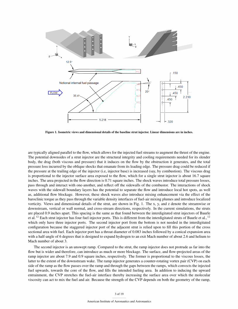
Figure 1. Isometric views and dimensional details of the baseline strut injector. Linear dimensions are in inches.

are typically aligned parallel to the flow, which allows for the injected fuel streams to augment the thrust of the engine.The potential downsides of a strut injector are the structural integrity and cooling requirements needed for its slenderbody, the drag (both viscous and pressure) that it induces on the flow by the obstruction it generates, and the totalpressure loss incurred by the oblique shocks that emanate from its leading edge. The pressure drag could be reduced ifthe pressure at the trailing edge of the injector (i.e, injector base) is increased (say, by combustion). The viscous dragis proportional to the injector surface area exposed to the flow, which for a single strut injector is about 16.7 squareinches. The area projected in the flow direction is 0.71 square inches. The shock waves introduce total pressure losses,pass through and interact with one-another, and reflect off the sidewalls of the combustor. The interactions of shockwaves with the sidewall boundary layers has the potential to separate the flow and introduce local hot spots, as wellas, additional flow blockage. However, these shock waves also introduce mixing enhancement via the effect of thebaroclinic torque as they pass through the variable density interfaces of fuel-air mixing plumes and introduce localizedvorticity. Views and dimensional details of the strut, are shown in Fig. 1. The x, y, and z denote the streamwise ordownstream, vertical or wall normal, and cross-stream directions, respectively. In the current simulations, the strutsare placed 0.9 inches apart. This spacing is the same as that found between the interdigitated strut injectors of Baurleet al.12 Each strut injector has four fuel injector ports. This is different from the interdigitated struts of Baurle et al.,12

which only have three injector ports. The second injector port from the bottom is not needed in the interdigitatedconfiguration because the staggered injector port of the adjacent strut is relied upon to fill this portion of the crosssectional area with fuel. Each injector port has a throat diameter of 0.083 inches followed by a conical expansion areawith a half-angle of 6 degrees that is designed to expand hydrogen to an exit Mach number of about 2.6 and helium toMach number of about 3.

The second injector is an unswept ramp. Compared to the strut, the ramp injector does not protrude as far into theflow but is wider and therefore, can introduce as much or more blockage. The surface, and flow-projected areas of theramp injector are about 7.9 and 0.9 square inches, respectively. The former is proportional to the viscous losses, thelatter to the extent of the downstream wake. The ramp injector generates a counter-rotating vortex pair (CVP) on eachside of the ramp as the flow passes over the ramp and through the gaps between the ramps, which convects the injectedfuel upwards, towards the core of the flow, and fills the intended fueling area. In addition to inducing the upwardentrainment, the CVP stretches the fuel-air interface thereby increasing the surface area over which the molecularviscosity can act to mix the fuel and air. Because the strength of the CVP depends on both the geometry of the ramp,

3 of 19


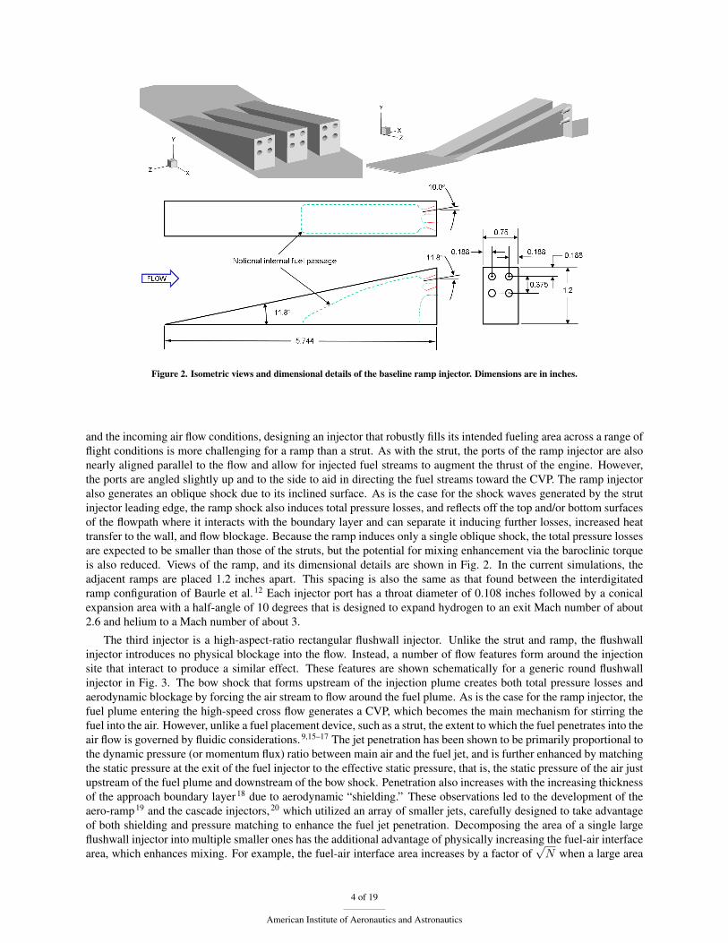
Figure 2. Isometric views and dimensional details of the baseline ramp injector. Dimensions are in inches.

and the incoming air flow conditions, designing an injector that robustly fills its intended fueling area across a range offlight conditions is more challenging for a ramp than a strut. As with the strut, the ports of the ramp injector are alsonearly aligned parallel to the flow and allow for injected fuel streams to augment the thrust of the engine. However,the ports are angled slightly up and to the side to aid in directing the fuel streams toward the CVP. The ramp injectoralso generates an oblique shock due to its inclined surface. As is the case for the shock waves generated by the strutinjector leading edge, the ramp shock also induces total pressure losses, and reflects off the top and/or bottom surfacesof the flowpath where it interacts with the boundary layer and can separate it inducing further losses, increased heattransfer to the wall, and flow blockage. Because the ramp induces only a single oblique shock, the total pressure lossesare expected to be smaller than those of the struts, but the potential for mixing enhancement via the baroclinic torqueis also reduced. Views of the ramp, and its dimensional details are shown in Fig. 2. In the current simulations, theadjacent ramps are placed 1.2 inches apart. This spacing is also the same as that found between the interdigitatedramp configuration of Baurle et al.12 Each injector port has a throat diameter of 0.108 inches followed by a conicalexpansion area with a half-angle of 10 degrees that is designed to expand hydrogen to an exit Mach number of about2.6 and helium to a Mach number of about 3.

The third injector is a high-aspect-ratio rectangular flushwall injector. Unlike the strut and ramp, the flushwallinjector introduces no physical blockage into the flow. Instead, a number of flow features form around the injectionsite that interact to produce a similar effect. These features are shown schematically for a generic round flushwallinjector in Fig. 3. The bow shock that forms upstream of the injection plume creates both total pressure losses andaerodynamic blockage by forcing the air stream to flow around the fuel plume. As is the case for the ramp injector, thefuel plume entering the high-speed cross flow generates a CVP, which becomes the main mechanism for stirring thefuel into the air. However, unlike a fuel placement device, such as a strut, the extent to which the fuel penetrates into theair flow is governed by fluidic considerations.9,15–17 The jet penetration has been shown to be primarily proportional tothe dynamic pressure (or momentum flux) ratio between main air and the fuel jet, and is further enhanced by matchingthe static pressure at the exit of the fuel injector to the effective static pressure, that is, the static pressure of the air justupstream of the fuel plume and downstream of the bow shock. Penetration also increases with the increasing thicknessof the approach boundary layer18 due to aerodynamic “shielding.” These observations led to the development of theaero-ramp19 and the cascade injectors,20 which utilized an array of smaller jets, carefully designed to take advantageof both shielding and pressure matching to enhance the fuel jet penetration. Decomposing the area of a single largeflushwall injector into multiple smaller ones has the additional advantage of physically increasing the fuel-air interfacearea, which enhances mixing. For example, the fuel-air interface area increases by a factor of

√N when a large area

4 of 19


Figure 3. Side and isometric views of the flow features that form around a generic flushwall injector during transverse injection of fuel intothe supersonic cross-stream. From Gruber et al. 14

is decomposed into N equal parts. Nevertheless, even these advanced concepts have limited application when scalingto larger flowpaths and operating at off-design conditions.

The flushwall injector exit geometry is based on the multi-objective optimization work of Ogawa21 whose approachusing a genetic algorithm revealed four families of high performing flushwall injectors. The injector port chosen forthe current work has a constant width, rectangular cross-section, with an aspect ratio of 8 at the injector exit plane, andthe longer dimension aligned in the streamwise direction. The injector is also inclined at 30 degrees to the wall. Theisometric views of the flushwall injector are shown in Fig. 4. The injector has been further designed to qualitativelymatch the geometrical features of the fuel ports of the strut injector. As such, the flushwall injector contains anexpansion section with a 6 degrees half-angle, and an expansion area ratio matching that of the strut conical fuel port.The area at the end of the expansion section, but before the 30 degrees rotation, has been adjusted to match the totalexit area of the 4 fuel ports of the strut. The width of the injector is 0.1392 inches with a throat height of 0.1541 inches.The adjacent flushwall injectors are placed 1.704 inches apart. This spacing corresponds to about 6 times the diameterof a circular injector with an equivalent area, and about 1.5 times the length of the current injector, allowing for asufficient air-gap between the adjacent injectors even after the expected axis-switching of the fuel plume.21

It should be noted that because the current simulations are for an open plate configuration, they do not take intoaccount the area expansion that is sometimes used to relieve the area blockage introduced into a ducted flowpath bystruts, ramps, or the aero-dynamic effects of the flushwall injection. In addition to counteracting the area blockage,this area relief causes the flow to expand through the gaps between the injectors and further enhance the strength ofthe CVP for the ramp configurations. Furthermore, the area expansion naturally ends at the base of the injector wherethe combustor walls typically turn parallel again (or continue at a very shallow angle of up to few degrees). Thisturning of the flow induces a shock wave at the base of the injector, which introduces additional total pressure lossesbut also enhances the fuel-air mixing via baroclinic torque effects, as discussed earlier. However, although potentiallybeneficial with respect to the mixing enhancement, the use of any flow expansions inside the combustor operatingat high Mach numbers would lead to increased Rayleigh losses due to chemical reactions because the heat additionwould occur at a higher value of the Mach number. Furthermore, the lower combustor static pressure could impact thecombustion efficiency in a way that might offset any benefits associated with mixing enhancement.

The inflow conditions correspond to a total pressure and total temperature of 4.31 MPa (625 psi) and 978 K(1760 ◦R), respectively, expanded to a Mach number of 6.36. A non-reacting, thermally perfect mixture of 21%oxygen (O2), 78% nitrogen (N2), and 1% nitric oxide (NO) by volume was used for the air. A small amount of NOwas present to account for production of this species in the experimental facility,22 although its impact on the currentsimulations is expected to be negligible. The fuel mass flow rate of helium for each injector was computed by assumingan equivalence ratio of one over the intended fueling area as if it were fueled with hydrogen. An intended fueling areais established independently for each injector. For example, a combustor cross-section area fueled with slender strutswill likely require such devices to be spaced more closely than a similar combustor fueled with large vortex generatingramps. Therefore, the intended fueling area will be narrower for struts than for the ramps. The intended fuelingareas for the strut and ramp are obtained from Baurle et al.12 who considered them in a realistic scramjet combustorconfiguration. Since the flushwall injector was designed with the intent to fuel the same flowpath, the intended fuelingarea height for the flushwall injector is the same as that for the strut with the width obtained from the optimization

5 of 19


Figure 4. Isometric views and dimensional details of the baseline flushwall injector.

work of Ogawa.21 The details of all of the flow parameters used in the current simulations are shown in Table 1. Boththe properties of air and fuel are presented. The subscripts f and a denote fuel and air flow streams, respectively. Inaddition to the quantities needed for the simulations, a few nondimensional quantities are also shown; these are, theunit Reynolds numbers per inch for the air and fuel streams, velocity difference parameter, ∆U, the convective Machnumber, Mc, and the ratios of the density, ρf / ρa, static pressure, pf / pa, and dynamic pressure, J between the fueland air stream. All values are computed based on the combustor entrance flow conditions for the air and the expandedflow conditions at the exit of the injector ports for the fuel. The nondimensional quantities have been found to berelevant to the injection and mixing processes in canonical problems.3,23,24

III. Metrics of Interest

A number of different metrics for thrust performance, mixing and combustion efficiency, and associated thermo-dynamic losses exist with the most detailed analysis proposed by Riggins et al.25 For the current study, the followingwere chosen: the integrated (in the cross-stream and vertical directions) forms of the total pressure recovery, mix-ing efficiency based on stoichiometric proportions of fuel and air, and thrust potential. The total mass-flux-weightedpressure recovery is defined as:

P rect =

∫PtρUdA∫

Pt∞ρUdA(1)

where Pt is the total pressure, ρ is the density, U and dA are the velocity magnitude and the incremental area projectedin the streamwise direction, respectively. This parameter is proportional to the difference between sensible entropiescomputed at the total and static values of the temperature, and therefore, gives a measure of the thermodynamic

6 of 19


Table 1. Global parameters of interest for the strut, ramp, and flushwall injector configurations. The last set of rows contain ratios ofinterest between the fuel (helium) and air streams, where the subscripts f and a denote fuel and air streams, respectively.

Property Air† Strut Ramp FlushwallMach 6.356 2.977 2.956 2.977

P0 (MPa) 4.309 0.224 0.0882 0.424T0 (K) 977.8 293.15 293.15 293.15P (kPa) 1.808 7.205 2.9114 13.642T (K) 112.4 74.14 74.91 74.14u (m/s) 1352.6 1508.2 1505.6 1508.2

Re/in x10e6 315.0 352.6 139.8 667.6Area‡ 0.9in x 2.25in 1.2in x 2.25in / 2 1.704in x 2.25in

ma (kg/s) x10e-3 98.76 65.84 187.00mf (kg/s) x10e-3 2.884 1.922 5.460

∆U§ 0.0544 0.0535 0.0544Mc

¶ 0.2163 0.2119 0.2163ρf / ρa 0.8371 0.3348 1.5849pf / pa 3.9845 1.6100 7.5440

J‖ 1.0408 0.4149 1.9706

†21% O2, 78% N2, 1% NO

‡Intended fueling area for the injector§Velocity difference parameter, ∆U = (uf − ua)/(uf + ua)

¶Convective Mach number, Mc = |uf − ua|/(cf + ca), c denotes the speed of sound.

‖Dynamic pressure ratio, J = (ρf u2f )/(ρau2

a) = (mf uf )/(maua).

losses. For purely mixing simulations, the total pressure recovery quantifies the losses due to the drag on the injectorbodies and the surface of the flat plate, the mechanical stirring induced by injector bodies (especially the ramp), theturbulence, the molecular mixing, and shock wave losses. For reacting simulations, the total pressure recovery isfurther reduced by the chemical reactions, therefore, the values of the total pressure recovery obtained from the non-reacting simulations could be thought of as the maximum achievable for a given injector. Because chemical reactionsreduce the total pressure recovery, which can be interpreted as a loss, yet energize the flow via heat release, which canbe expanded into thrust, there is a need for another metric that more objectively quantifies the potential performanceof the flowpath. The most direct metric that can achieve this is the thrust potential. This metric is obtained at eachstreamwise location by first one-dimensionalizing the flow at that location, and then allowing it to expand isentropicallythrough an ideal thrust nozzle. In the current work, this thermodynamic process is evaluated until the flow reaches itscombustor entrance value of the static pressure. The thrust potential is defined here by

TP (N) = muexit + (pexit − p3)Aexit (2)

where TP is the thrust potential, and m, uexit, pexit, Aexit, and p3 are the mass flow rate, velocity, pressure, and thearea at the thrust nozzle exit plane, and the combustor entrance static pressure, respectively. Since the flow is expandedto the combustor entrance static pressure, the second term in the above equation is identically zero. Therefore, thismetric represents the momentum portion of the ideal potential thrust that could be obtained when a flowpath of interestis truncated at a given streamwise location and coupled at that location to an ideal thrust nozzle. All of the losses inthe value of the total pressure previously discussed for the purely mixing case would still appear as a decrement to thevalue of this thrust potential, however, the combustion heat release will increase the value of the thrust potential. Itshould be noted that the definition of the thrust potential is different from one used commonly when assessing vehicleperformance. This is because we are simulating only a portion of the vehicle flowpath for which it is difficult to definea meaningful thrust, yet we are interested in a metric that would be proportional to it.

The mixing efficiency is defined in this work following Mao et al.:16

ηm =∫

αRρUdA∫αρUdA

(3)

7 of 19


where the integration is over a single streamwise, x-plane of interest, and α is the fuel or oxidizer mass fractiondepending on whether the global equivalence ratio is less than or greater than 1, respectively. Quantity αR is definedas the amount of fuel or oxidizer that would react if complete reaction took place without further mixing, i.e.,

αR =

{α, α ≤ αst

αst

1−αst(1− α), α > αst

(4)

where αst is the stoichiometric value of fuel or oxidizer mass fraction. For cases with an overall equivalence ratio ofone, either fuel or oxidizer can be used in place of α. But choosing fuel has a minor benefit of clarifying somewhatthe meaning of Eq. (4), which becomes:

αR =

{Yf , Yf ≤ Yf,st

FARst Ya, Yf > Yf,st

(5)

where Y denotes mass fraction, FARst is the stoichiometric fuel to air ratio set to 0.0292 in the current work, andsubscripts f and a denote fuel and air streams, respectively. It is clear from the above equation that if the local valueof the mass fraction of fuel is less than its stoichiometric value, then that amount is “counted” as fully mixed becausethere is sufficient amount of air to completely deplete the fuel if reactions were allowed. However, if the local valueof the fuel mass fraction is greater than its stoichiometric value, then the only part that could react is that which isin stoichiometric proportion to the local value of the mass fraction of the air. Therefore, only that portion is countedas being mixed in Eq. (3). The stoichiometric value of the hydrogen mass fraction is 0.0285. The mixing efficiencyformula of Mao et al.16 can also be used to analyze mixing in the reacting simulations, however, since fuel and oxidizerare consumed to make combustion products, care must be taken to consider the elemental mass fractions of fuel oroxidizer (i.e., mass fractions of all elements that originate in either fuel or oxidizer streams).

IV. Numerical Considerations

The numerical simulations were performed using the Viscous Upwind aLgorithm for Complex flow ANalysis(VULCAN-CFD) code.26 VULCAN-CFD is a multi-block; structured-grid, cell-centered, finite-volume solver widelyused for all-speed flow simulations. For this work, Reynolds-averaged simulations (RAS) were performed. Theadvective terms were computed using a Monotonic Upstream-Centered Scheme for Conservation Laws (MUSCL)scheme27 with the Low-Dissipation Flux-Split Scheme (LDFSS) of Edwards.28 The thermodynamic properties ofthe mixture components were computed using curve fits of McBride et al.29 The governing equations were integratedusing an implicit diagonalized approximate factorization (DAF) method.30 The current work used the baseline blendedk− ω/k− ε turbulent physics model of Menter.31 The Reynolds heat and species mass fluxes were modeled usinga gradient diffusion model with turbulent Prandtl and Schmidt numbers of 0.9 and 0.5, respectively. Wilcox wallmatching functions32 were also used, however, their implementation in VULCAN-CFD includes a modification thatallows the simulations to recover the integrate-to-the-wall behavior as the value of y+ approaches one. All simulationswere converged until the total integrated mass flow rate and the total integrated heat flux on the walls remainedconstant. This typically occurred when the value of the L2-norm of the steady-state equation-set residual decreased byabout 4–5 orders of magnitude. To conserve the available computational resources, all the simulations were split intoan elliptic and a space-marching region. The elliptic region contained the inflow of the domain, the injector bodies, andup to 6.5 inches downstream of the injection plane. The computational cell count was about equal in both regions, butthe computational cost associated with solving the space-marching regions was about an order of magnitude lower thanthat for the elliptic region. A single, fully elliptic simulation on a coarse grid confirmed that this approach indeed didnot have a significant impact on any of the flow features nor the integrated values of the metrics of interest discussedin the previous section.

Three grids, coarse, medium, and fine, each progressively finer by a factor of 2 in each of the three dimensions,were used. The grid resolutions are summarized for the three injector types in Table 2. For the strut injector, asingle full strut injector was included in the computational domain. This was done to help alleviate some of thegrid skewness issues at the top of the strut, and near the leading edge of the strut. For the ramp injector case, onlyhalf of the ramp injector was included in the computational domain, taking advantage of the symmetry to reducethe grid size requirement. Similarly, the flushwall injector simulations also used only half of the full domain. Allgrids were generated with GridPro in the vicinity of the injector bodies and the leading edge of the flat plate, and

8 of 19


further combined with Pointwise-generated h-blocks to complete the computational definition of the geometry. For allinjectors, the inflow and outflow planes are placed 9 inches upstream, and 25 inches downstream of the fuel injectionplane, which is located at x = 0. Since both the inflow and the outflow consist of supersonic flow, static values of thetemperature and pressure, and the Mach number are specified at the inflow; and all flow variables are extrapolated atthe outflow. The vertical dimension is 6 inches high, which approximates the size of the EIMP facility nozzle coreflow.33 Slip wall boundary conditions are used for the upper boundary of the flow domain. This was done to accountfor the presence of the facility nozzle jet stretchers used in the EIMP experiments. Since the boundary layer along thejet stretchers is of little interest and is not expected to impact the mixing region, no attempt was made to resolve andmodel it in the current simulations. Since the simulation domain effectively includes an infinite row of injectors in thecross-stream, the current simulations model the open plate experiment as a wide duct. In this model duct, the flowblockage due to injector bodies is 14% and 12.5% for the strut and ramp injectors, respectively. With the exception ofthe fuel ports, the grid was clustered towards all of the walls with the growth rates varying from 5%–15%. The gridresolution study for the strut and ramp grids used in the current simulations have been previously reported by Drozdaet al.11 The values of y+ for these cases, obtained on a fine mesh, vary up to about 20, with the largest values observedon the injector bodies and fuel port walls. The y+ values along the flat plate are all less than one. The grid for theflushwall injector was built using the same density and near-wall spacing requirements as those for the strut and ramp,therefore the y+ values match those observed for the other cases. The values of y+ are about two and four times largerfor the medium and coarse meshes, respectively.

The one-dimensional values of the total pressure recovery and the mixing efficiency versus the downstream dis-tance in inches obtained from the simulations on the coarse, medium, and fine meshes are shown in Fig. 5. Due to thelimitation of the one-dimensional post-processor to analyze only axial planes of data, some plots contain gaps wherethe complicated grid topology contained streamwise grid “wraps”. These “wraps” could have been interpolated onto aCartesian mesh, however numerical interpolation of cell center quantities could have introduced additional errors thatwould be external to the solver. To avoid this, the “wrap” regions were omitted from the one-dimensional analysis.In addition, the grid independence study for the strut and ramp injectors were previously performed11 under differentflow conditions. Because these flow conditions corresponded to the higher values of the Reynolds numbers for boththe main air flow and the fuel ports, the study was deemed conservative with respect to the current conditions. But,because of the flow differences, the profiles for the mixing efficiency and the total pressure recovery for the strut andramp injectors reported in this section are shifted from those reported in the results section. The grid independencestudy shown for the rectangular injector has been performed under the flow conditions reported in Table 1. In addi-tion, unlike the strut and ramp injectors, which introduce all of the fuel at a single downstream location, the flushwallinjector has a downstream length over which the fuel is effectively distributed. This feature manifests itself in theone-dimensional plot as a rapid rise and decline in the value of the mixing efficiency because the value of the totalintegrated mass flow rate of the fuel gradually increases from the beginning of the injection plane until the downstreamedge of the flushwall injector.

The one-dimensional values of the total pressure recovery and the mixing efficiency change monotonically withincreasing grid resolution. However, the rate of convergence at which these values approach their asymptotic statevaries among the cases and with the downstream distance. This behavior is possibly due to the use of wall matchingfunctions on the injector bodies and inside the fuel ports. The behavior of these functions and the resulting boundarylayers change for different grid densities as the y+ values change. The error bars corresponding to the data obtained onthe fine mesh and shown in Fig. 5 were obtained assuming a unity order of accuracy and using the Grid ConvergenceIndex (GCI),34 which is based on Richardson extrapolation. The resulting error bars are proportional to the differencebetween the results obtained on the fine and medium meshes, and represent an estimate of the error bounds between thecurrent result and its fully grid-converged value. Although the formal order of accuracy of VULCAN-CFD is secondorder, unity order of accuracy was used for the GCI to ensure a conservative estimate of the errors. Furthermore,visual inspection of the differences between the one-dimensional values of the mixing efficiency, obtained from the

Table 2. Grid densities used in the current simulations.

Strut Ramp FlushwallCoarse 4,921,682 4,057,382 4,356,936

Medium 39,373,456 32,459,056 34,855,488Fine 314,987,648 259,672,448 278,843,904

9 of 19


(a) Strut (b) Ramp

(c) Flushwall

Figure 5. One-dimensional values of the total pressure recovery and mixing efficiency vs. downstream distance (in inches) obtained fromthe simulations on the coarse, medium, and fine grids, for the cases corresponding to the strut, ramp, and flushwall injectors.

simulations on the three different grids, reveals that these data appear to be converging slower than the formal orderof accuracy of the solver. It should be noted that this result is not a reflection of the formal order of accuracy ofthe VULCAN-CFD solver, but rather the impact of shocks on the flow field. To ensure smooth solution near theflow discontinuities and improve the simulation stability, the solver reverts to the unity order of accuracy near thesediscontinuities. The observed numerical errors in the values of the total pressure recovery have a maximum value ofabout 5%, with 1%–2% typical, and a maximum value of about 15% (in the near-field of the ramp injector case) with5% typical for the mixing efficiency. Because the errors in the 1D values of the quantities of interest approach limitstypically encountered in the engineering analysis, only the results of the simulations obtained on the fine meshes arepresented in the subsequent sections.

All of the current simulations were performed on the Pleiades Supercomputer located at NASA Ames. The com-putational cost associated with solving a single simulation on the fine mesh was about 60 k CPU hours. Simulations,

10 of 19


Figure 6. Contours of the Mach number on the z-planes obtained at the centerline, and half-way between the injectors, and x-planes atvarious downstream locations for the strut injector simulations. Downstream distance is in inches. Black lines denote the stoichiometricvalue of the fuel mass fraction.

were typically performed using 480 compute cores with most cases converging in 5 days. The total computational costof the study was about 1 million CPU hours, which included medium and coarse mesh simulations (about 100 k CPUhours), and pre- and post-processing of the fine mesh simulation results (about 10 k CPU hours).

V. Results and Discussion

Contour plots of the Mach number in the z-planes obtained through the center of the injector ports and midwaybetween the injectors, and x-planes at various locations for the strut and ramp injectors for all of the cases are shownin Figs. 6–8. The flow is left-to-right. For the x-planes, the aspect ratio is not one because these planes are viewedlooking aft-to-fore from an angle of about 30 degrees to the x-axis in the xz-plane. The streamwise distance on thesefigures is in inches. The black isocontour line denotes a helium mass fraction equal to the stoichiometric value forhydrogen (0.0285), which closely approximates the location of the peak heat release in reacting flows and furtherdelineates a boundary of our mixing metric of interest (Eq. (5)). The extent of mixing may be qualitatively observedby examining the extent of the area enclosed by this isocontour line. However, some care should be exercised wheninterpreting this area because the fuel will diffuse to its stoichiometric isocontour value only in the global sense (andafter long-time mixing or in the far-field). As the fuel and air mix in the near-field of the injector, there could existlocal mixing regions where the equivalence ratio is rich or lean. In the former, the area enclosed by the stoichiometricvalue will simply grow more slowly, but in the latter case this area will first grow and then shrink and collapse as thefuel mixes with air to locally sub-stoichiometric proportions.

Qualitatively, the flow features for all of the injectors are very similar. Upstream, the leading edge of the flat plate

11 of 19


Figure 7. Contours of the Mach number on the z-planes obtained through the center of the injector ports, and half-way between theinjectors, and x-planes at various downstream locations for the ramp injector simulations. Downstream distance is in inches. Black linesdenote the stoichiometric value of the fuel mass fraction.

causes a shallow bow shock at about 12.5 degrees to the flat plate, which is slightly larger than the Mach wave angleof about 9 degrees for this Mach number. The approach boundary layer thickness is a fraction of the height of boththe strut and the ramp injector bodies such that the side walls of both injectors are exposed to the free stream air flow.As a consequence, the boundary layers that develop on the sides of the injector bodies, just as the boundary layernear the leading edge of the flat plate, are thin and transitional, which makes them more susceptible to shock-inducedseparation. For the current turbulence model, the transition is expected to occur at a streamwise Reynolds number thatis about an order of magnitude lower than that found in most turbulent flows of engineering interest.32 Therefore, thesimulated flows are expected to become fully turbulent sooner than their realistic counterparts and will, therefore, bemore resilient to shock-induced separation.

For the strut injector, shown in Fig. 6, a cross-stream shock wave is generated by the sharp leading edge of thestrut injector body (e.g., at –3 inches). The turning half-angle of the strut injector body leading edge is 6.25 degrees(see Fig. 1), resulting in the leading edge shock wave angle of about 17 degrees as measured from the CFD. Becausethe leading edge of the strut body is swept at 35.4 degrees, the resulting oblique shock wave is reflected at somewhatlarger angle than that expected for the turning angle of 6.25 degrees. This shock wave propagates in the cross-streamdirection and impacts the body of the adjacent injector. This propagation is evident by the change in the value of theMach number at downstream locations between –3 and 0 inches on the middle plots of each figure. After the reflectionfrom the adjacent injector, the oblique shock waves continue to pass through one another and interact, leading to thecomplex downstream pattern seen in the figures. As these shock waves pass through the variable density fuel-airinterface, vorticity is produced locally due to the effect of the baroclinic torque. Although the baroclinic effects aregenerally small, this vorticity curves and stretches the local fuel-air interface regions, thereby increasing the fuel-air

12 of 19


Figure 8. Contours of the Mach number on the z-planes obtained through the center of the injector port, and half-way between theinjectors, and x-planes at various downstream locations for the flushwall injector simulations. Downstream distance is in inches. Blacklines denote the stoichiometric value of the fuel mass fraction.

mixing rate, albeit at the expense of total pressure losses. As the flow continues past the strut injector body, a counterrotating vortex pair (CVP) forms near the tip of the injector body. The top-most fuel port injects the fuel streamdirectly at the space between the CVP. The combined effect of the angled injection and the CVP distorts and bifurcatesthe top-most fuel stream, and separates it from those of the three lower parallel fuel ports. This effect can be seen byobserving the stoichiometric value of the mass fraction as it evolves in the x-planes in Fig. 6.

For the ramp injector, shown in Fig. 7, an oblique shock wave is generated by the inclined ramp surface of theramp injector body. The turning angle of the ramp surface is 11.8 degrees (see Fig. 2), resulting in the oblique shockwave angle of about 17 degrees at the injector centerline. The value of this angle is slightly reduced from the expectedvalue (of about 19 degrees) for this turning angle because of the interaction of the shock with the approach boundarylayer. This oblique shock interacts and coalesces with the same shock wave produced by the adjacent injector bodies.However, unlike the cross stream shock waves that emanate from the leading edge of the strut, the ramp body obliqueshock wave does not interact with the fuel-air mixing plume but instead serves primarily to introduce a pressuredifference between the top of the ramp surface and the gap between the adjacent injectors. The pressure is higher onthe ramp surface, which creates a driving force for the flow to spill from the ramp surface into the gap between theadjacent injectors. This spillage introduces counter rotating vortices on either side of the ramp injector body with thesize proportional to the ramp height. These vortices are large compared to the size of the fuel ports. Therefore, whenthey begin to interact with the injected fuel streams, they stretch and push the fuel-air interface upwards away from theplate boundary layer and into the core of the flow. This process is further aided by the fact that all the ramp fuel portsare angled at 11.8 degrees up and the top set is angled at 10 degrees outwards towards the gap between the adjacentinjectors. The combined effect of the angled injection and the large-scale CVP spreads the fuel through the intended

13 of 19


fueling area. These effects can be seen by observing the stoichiometric value of the mass fraction as it evolves in thex-planes in Fig. 7.

For the flushwall injector, shown in Fig. 8, the flow features and dynamics are somewhat similar to that of the rampinjector. An oblique bow shock wave is generated by the fuel entering into the supersonic cross-stream. The obliqueshock wave angle is about 16 degrees at the injector centerline. This bow shock interacts and joins with the samebow shock wave produced by the adjacent injector fuel plumes. Similar to the shock generated by the ramp body,the flushwall injector oblique shock wave does not significantly interact with the fuel-air mixing plume but insteadserves primarily to introduce a pressure difference between the top of the fuel plume and the gap between the adjacentinjectors. The pressure is higher on the top of the plume, which creates a driving force to form a CVP around thefuel plume. This CVP is too weak to significantly deform the stoichiometric isosurface, nevertheless it does providean upward lifting force as the fuel is convected downstream. A secondary CVP also forms inside the stoichiometricisocontour line. This CVP is driven by the underexpanded fuel plume penetrating into the supersonic cross-flow andcan be seen at x = 3 station on Fig. 8. Because the flushwall injector is underexpanded (see Table 1) the fuel plumespreads laterally in addition to penetrating into the cross-flow. The underexpansion process “redistributes” some ofthe dynamic pressure (or momentum) of the fuel jet laterally, thereby reducing the amount available for cross-flowpenetration. Nevertheless, the penetration is comparable to that of the ramp injector. The primary difference betweenthe flushwall injection and that using a strut or a ramp is that a significant amount of fuel remains in the boundary layer.The fact that the fuel contacts the wall reduces the fuel-air interface area (and mixing) as compared to a fully liftedfuel plume. Furthermore, depending on the wall temperature, the combustion could be quenched by the wall, therebypreventing the extraction of exothermic energy from the fuel. However, if combustion does occur in the boundarylayer it would increase the thermal loads on the wall but at the same time provide some means of flame-holding. Inaddition, Chan et al.35 have reported evidence of drag reduction by near-wall burning.

Plots of the one-dimensional values of the mass-flux-weighted average Mach number, and mixing efficiency versusdistance in inches are shown in Fig. 9 for the strut, ramp, and flushwall injectors. These plots help to quantify theoverall behavior of the flow and the level of mixing found among all of the simulated cases. Considering the onedimensional value of the Mach number first, the results indicate that the Mach number decreases throughout the flow.The decreases are caused by the effect of the shock waves and friction losses throughout the flowpath and by themixing losses downstream of the injection plane. The shock waves and drag losses induced by the strut and rampinjector bodies are evident by a more significant decrease in the Mach number at the injection plane, and the overalloffset of values, as compared to the flushwall injector. Downstream of the injection plane the profiles of the Machnumber for the strut and ramp injectors appear to follow a slightly stair-stepping pattern. This effect is caused by theshock waves crossing through, reflecting, and interacting with the mixing plume and is most pronounced in the strutinjector case.

The mixing efficiency results are consistent with the observations of the Mach number contours and the corre-sponding areas enclosed by the stoichiometric values of the fuel species elemental mass fractions. The fuel and airmix the fastest for the strut injector, followed by the ramp, and the flushwall injectors. The profiles corresponding tothe strut and ramp exhibit three distinct mixing regions. The first region, in the near-field of the injector body from0 to about 2 inches (or about an injector body height), is characterized by a rapid rise in the mixing efficiency. Thelength of this region also correlates with the wake generated by the injector bodies. The fuel injected into this wakeregion has more time to mix with the surrounding air. This region is followed by a fairly long region where the mixingefficiency increases less rapidly and linearly with the downstream distance. The third region begins at about 22 inchesand is characterized by a further decrease in the mixing rate. Unlike the strut and ramp injectors, the flushwall injectorexhibits a linear increase in the mixing efficiency with the downstream distance.

Figure 10 shows the one-dimensional values of the mass-flux-weighted average axial vorticity magnitude, andthe turbulence kinetic energy (TKE). The former is proportional to the circulation, which is a measure of large scalerotating motions in the cross-stream planes. The latter is an indicator of the intensity of the turbulence motions.Both quantities are indicative of the potential for the large vortical structures and the turbulence motions, respectively,to distort and wrinkle the fuel-air interface area, and enhance mixing. The strut injector body induces the largestamount of axial vorticity. This vorticity is produced near the tip of the strut, as well as, on the sides by the cross-stream pressure differences induced by the complex patterns of interacting shock waves. Downstream of the strutinjector body additional vorticity is produced by the expanding fuel plumes, which redistribute the initially axialmomentum laterally, thereby producing additional cross-stream vorticity near the fuel-air interface. The strut injectoralso generates the largest amount of turbulent fluctuations, which indicates that turbulent motions are most intense forthis injector.

14 of 19


Figure 9. One-dimensional values of the Mach number, and mixing efficiencies vs. the downstream distance (in inches).

Figure 10. One-dimensional values of the axial (unit vector n is oriented in the streamwise direction) vorticity magnitude (1/s), and theturbulence kinetic energy (m2/s2) vs. the downstream distance (in inches).

The ramp and flushwall injectors produce comparable amounts of both axial vorticity and turbulence intensity.The axial vorticity corresponding to the ramp injector is dominated by the large scale vortex associated with the ramp-induced CVP. The flushwall injector produces two relatively large CVPs, first directly behind the bow shock, and asecond inside and around the fuel plume due to underexpansion (as discussed earlier). Despite a comparable amountof vortical and turbulent motions, and penetration (as see in Figs. 7, and 8), the mixing efficiency of the flushwallinjector is significantly less than that for the ramp injector. This indicates that both the bluff-body flow separation andthe wake produced by the ramp injector body, which increase the residence time for the fuel and air mixing, have asignificant impact on the rate of mixing.

The total pressure recovery profiles are shown in Fig. 11. Because the total pressure is proportional to the entropy,

15 of 19


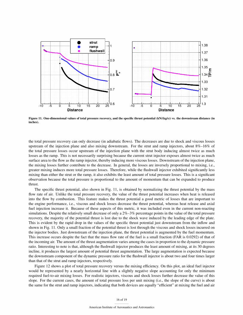
Figure 11. One-dimensional values of total pressure recovery, and the specific thrust potential (kN/(kg/s)) vs. the downstream distance (ininches).

the total pressure recovery can only decrease (in adiabatic flows). The decreases are due to shock and viscous lossesupstream of the injection plane and also mixing downstream. For the strut and ramp injectors, about 8%–16% ofthe total pressure losses occur upstream of the injection plane with the strut body inducing almost twice as muchlosses as the ramp. This is not necessarily surprising because the current strut injector exposes almost twice as muchsurface area to the flow as the ramp injector, thereby inducing more viscous losses. Downstream of the injection plane,the mixing losses further contribute to the decrease. In general, the losses are inversely proportional to mixing, i.e.,greater mixing induces more total pressure losses. Therefore, while the flushwall injector exhibited significantly lessmixing than either the strut or the ramp, it also exhibits the least amount of total pressure losses. This is a significantobservation because the total pressure is proportional to the amount of momentum that can be expanded to producethrust.

The specific thrust potential, also shown in Fig. 11, is obtained by normalizing the thrust potential by the massflow rate of air. Unlike the total pressure recovery, the value of the thrust potential increases when heat is releasedinto the flow by combustion. This feature makes the thrust potential a good metric of losses that are important tothe engine performance, i.e., viscous and shock losses decrease the thrust potential, whereas heat release and axialfuel injection increase it. Because of these aspects of this metric, it was included even in the current non-reactingsimulations. Despite the relatively small decrease of only a 2%–3% percentage points in the value of the total pressurerecovery, the majority of the potential thrust is lost due to the shock wave induced by the leading edge of the plate.This is evident by the rapid drop in the values of the specific thrust potential just downstream from the inflow andshown in Fig. 11. Only a small fraction of the potential thrust is lost through the viscous and shock losses incurred onthe injector bodies. Just downstream of the injection plane, the thrust potential is augmented by the fuel momentum.This increase occurs despite the fact that the mass flow rate of the fuel is a small fraction (FAR is 0.0292) of that ofthe incoming air. The amount of the thrust augmentation varies among the cases in proportion to the dynamic pressureratio. Interesting to note is that, although the flushwall injector produces the least amount of mixing, at its 30 degreesincline, it produces the largest amount of potential thrust augmentation. The large augmentation is expected becausethe downstream component of the dynamic pressure ratio for the flushwall injector is about two and four times largerthan that of the strut and ramp injectors, respectively.

Figure 12 shows a plot of total pressure recovery versus the mixing efficiency. On this plot, an ideal fuel injectorwould be represented by a nearly horizontal line with a slightly negative slope accounting for only the minimumrequired fuel-to-air mixing losses. For realistic injectors, viscous and shock losses further decrease the value of thisslope. For the current cases, the amount of total pressure loss per unit mixing (i.e., the slope of the curve) is aboutthe same for the strut and ramp injectors, indicating that both devices are equally “efficient” at mixing the fuel and air

16 of 19


Good Mixing�

��

Poor Mixing

��

��

Figure 12. One-dimensional values of the total pressure recovery vs. mixing efficiency.

under the current conditions. The downward offset of strut profile is a result of the greater total pressure losses incurredon the strut injector body. Nevertheless, these larger losses are indeed converted into greater mixing, as indicated by alarger final value of the mixing efficiency for the strut as compared to both the ramp and a flushwall injectors.

The flushwall injector is less efficient at near-field mixing. The rapid decrease in the total pressure recovery forthe flushwall injector includes the bow shock losses, which for the strut and ramp injectors occurred upstream of theinjection plane at the leading edges of their respective injector bodies. For these injectors, the upstream losses arenoted on the plot at the mixing efficiency of zero. Nevertheless, unlike the strut injector, the significant, early totalpressure losses for the flushwall injector do not result in a corresponding increase in the value of the mixing efficiency.However, the final slope of the profile does approach that for the ramp and the strut, indicating a comparable rate oftotal pressure loss vs. mixing in the far-field.

Overall, the flushwall injector and its downstream mixing field induce less total pressure loss than those for thestrut and ramp. However, the amount of mixing induced at a given downstream distance is also significantly lower, butthe thrust potential is the largest. Such trade-offs, when considered together with the other factors such as combustion,which increase the thrust potential in proportion to the mixing (and combustion) efficiency, make comparisons betweenthe different injectors quite complicated, and ultimately may prove to require considering a ducted flowpath, thatincludes space-filling injector arrangements, together with the knowledge of the specific flight trajectory.

VI. Conclusions

The CFD analysis based on Reynolds-Averaged Simulations (RAS) is presented of the mixing characteristics,performance, and trade-offs of three types of fuel injectors at hypervelocity flow conditions. The injectors consist of afuel placement device, a strut; a fluidic vortical mixer, a ramp; and a geometrically-optimized21 flushwall injector. Thestrut injector has a slender, swept, body protruding into the core of the flowpath, the ramp injector produces a largevortex using an unswept ramp, and the flushwall injector is a downstream-oriented high-aspect-ratio rectangle inclinedto the wall to augment the thrust. These choices represent three main categories of injectors typically considered inthe propulsive devices used for high-speed flight. The contours of the Mach number obtained from the RAS revealedthe qualitative mixing characteristics for the three injectors. It was found that: the strut injector induced the most rapid

17 of 19


mixing; the ramp-induced counter-rotating vortex pair was not sufficient to enhance upward fuel penetration, but thefuel was injected and remained above the boundary layer; and even with penetration comparable to that of the ramp, theflushwall injector introduced a significant amount of fuel into the boundary-layer. The one-dimensional values of themass-flux-weighted average Mach number, mixing efficiencies, total pressure recovery, and specific thrust potential, aswell as, mass-flux-weighted average axial vorticity, and turbulence kinetic energy, were used to quantify the differencesamong the injectors. These quantities showed that although the strut injector produced the greatest amount of fuel-to-air mixing, it did so at the expense of significant total pressure losses. On the other hand, the flushwall injector,which produced the least amount of mixing, exhibited the greatest value of the specific thrust potential augmentationbecause of its large dynamic pressure. The one-dimensional plots of the total pressure recovery vs. mixing efficiencyshowed that the mixing “efficiency” rates (i.e., the slope of these curves) for the mixing fields corresponding to thestrut and ramp injectors are comparable, and that the flushwall injector approaches this value in the far-field. Theprimary goal of the current work is not to pinpoint the best fuel injector for hypervelocity flow applications but ratherto discuss physical considerations, and illustrate and highlight the many competing factors related to fuel injection thatmay impact the eventual injector performance at any flow conditions. The current analysis highlights the challengesassociated with selecting the “best” injector in the presence of competing factors, i.e., maximizing mixing efficiency,total pressure recovery, and thrust potential. Future work will utilize the current injectors in ducted configurations withhydrogen fuel and chemical reactions.

Acknowledgments

Many stimulating discussions with Dr. Richard L. Gaffney Jr. on the subject of high-speed injection and mixingare gratefully acknowledged. This work is supported by the Hypersonic Airbreathing Propulsion sub-project of theAeronautics Evaluation and Test Capabilities Project of the Advanced Air Vehicles Project in the NASA AeronauticsResearch Mission Directorate (ARMD). Computational resources are provided by the NASA Langley Research Centerand the NASA Advanced Supercomputing (NAS) Division.

References1Peebles, C., Road to Mach 10: Lessons Learned From the X-43A Flight Research Program, Library of Flight Series, AIAA, Washington,

D.C., 2008.2Hank, J.M., Murphy, J.S., and Mutzman, R.C., “The X-51A Scramjet Engine Flight Demonstration Program,” in 15th AIAA International

Space Planes and Hypersonic Systems and Technologies Conference, AIAA, Dayton, OH, 2008.3Papamoschou, D. and Roshko, A., “The Compressible Turbulent Shear Layer: An Experimental Study,” J. Fluid Mech., Vol. 197, 1988, pp.

453–477.4Givi, P., Madnia, C.K., Steinberger, C.J., Carpenter, M.H., and Drummond, J.P., “Effects of Compressibility and Heat Release in a High

Speed Reacting Mixing Layer,” Combust. Sci. Technol., Vol. 78, 1991, pp. 33–68.5Drummond, J.P., Carpenter, M.H., and Riggins, D.W., “Mixing and Mixing Enhancement in Supersonic Reacting Flow Fields,” in S.N.B.

Murthy and E.T. Curran, eds., High Speed Propulsion Systems, Vol. 137 of AIAA Progress Series, chap. 7, American Institute of Aeronautics andAstronautics, 1991, pp. 383–455.

6Drummond, J.P. and Givi, P., “Suppression and Enhancement of Mixing in High-Speed Reacting Flow Fields,” in J.D. Buckmaster, T.L.Jackson, and A. Kumar, eds., Combustion in High-Speed Flows, Kluwer Academic Publishers, Netherlands, 1994, pp. 191–229.

7Vreman, A.W., Sandham, N.D., and Luo, K.H., “Compressible Mixing Layer Growth Rate and Turbulence Characteristics,” J. Fluid Mech.,Vol. 320, 1996, pp. 235–258.

8Foysi, H. and Sarkar, S., “The Compressible Mixing Layer: An LES Study,” Theor. Comp. Fluid. Dyn., Vol. 24, 2010, pp. 565–588.9Lee, J., Lin, K.C., and Eklund, D., “Challenges in Fuel Injection for High-Speed Propulsion Systems,” AIAA J., Vol. 53, No. 6, 2015, pp.

1405–1423.10McClinton, C.R., “Evaluation of Scramjet Combustor Performance Using Cold Nonreactive Mixing Tests,” in 14th AIAA Aerospace Sciences

Meeting, Washington, DC, 1976.11Drozda, T.G., Baurle, R., and Drummond, J.P., “Impact of Flight Enthalpy, Fuel Simulant, and Chemical Reactions on the Mixing Char-

acteristics of Several Injectors at Hypervelocity Flow Conditions,” in 63rd JANNAF Propulsion Meeting / 47th CS / 35th APS / 345h EPSS / 29thPSHS Joint Subcommittee Meeting, Newport News, VA, 2016.

12Baurle, R.A., Fuller, R.P., White, J.A., Chen, T.H., Gruber, M.R., and Nejad, A.S., “An Investigation of Advanced Fuel Injection Schemesfor Scramjet Combustion,” in 36th Aerospace Sciences Meeting and Exhibit, Reno, NV, 1998.

13Cabell, K., Drozda, T.G., Axdahl, E.L., and Danehy, P.M., “The Enhanced Injection and Mixing Project at NASA Langley,” in JANNAF46th CS / 34th APS / 34th EPSS / 28th PSHS Joint Subcommittee Meeting, Albuquerque, NM, 2014.

14Gruber, M.R., Nejad, A.S., and Dutton, J.C., “Circular and Elliptical Transverse Injection into a Supersonic Crossflow – The Role ofLarge-Scale Structures,” in 26th Fluid Dynamics Conference, San Diego, CA, 1995.

18 of 19


15Schetz, J.A. and Billig, F.S., “Penetration of Gaseous Jets Injected into a Supersonic Stream,” J Spacecraft Rockets, Vol. 3, No. 11, 1966,pp. 1658–1665.

16Mao, M., Riggins, D.W., and McClinton, C.R., “Numerical Simulation of Transverse Fuel Injection,” in Computational Fluid DynamicsSymposium on Aeropropulsion, NASA-CP-3078, NASA, Cleveland, OH, 1990, pp. 635–667.

17Portz, R. and Segal, C., “Penetration of Gaseous Jets in Supersonic Flows,” AIAA J, Vol. 44, No. 10, 2006, pp. 2426–2429.18McClinton, C.R., “Effect of Ratio of Wall Boundary-Layer Thickness to Jet Diameter on Mixing of a Normal Hydrogen Jet in Supersonic

Stream,” NASA Technical Memorandum NASA TM X-3030, NASA, Hampton, VA, 1974.19Maddalena, L., Campioli, T.L., and Schetz, J.A., “Experimental and Computational Investigation of an Aeroramp Injector in a Mach Four

Cross Flow,” in AIAA 13th International Space Planes and Hypersonic Systems and Technologies Conference, AIAA 2005-3235, 2005.20Cox-Stouffer, S., Gruber, A., and Bulman, M.J., “A Strealined, Pressure-Matched Fuel Injector for Scramjet Applications,” in 36th

AIAA/ASME/SAE/ASEE Joint Propulsion Conference and Exhibit, AIAA 2000-3707, AIAA, Huntsville, AL, 2000.21Ogawa, H., “Physical Insight into Fuel-Air Mixing for Upstream-Fuel-Injected Scramjets via Multi-Objective Design Optimization,” J

Propul Power, Vol. 31, No. 6, 2015, pp. 1505–1523.22Cabell, K.F. and Rock, K.E., “A Finite Rate Chemical Analysis of Nitric Oxide Flow Contamination Effects on Scramjet Performance,”

Tech. Rep. TP-212159, NASA, 2003.23Brown, G.L. and Roshko, A., “On Density Effects and Large Structure in Turbulent Mixing Layers,” J. Fluid Mech., Vol. 64, 1974, pp.

775–816.24Bogdanoff, D.W., “Compressibility Effects in Turbulent Shear Layers,” AIAA J., Vol. 21, No. 6, 1983, pp. 926–927.25Riggins, D.W., McClinton, C.R., and Vitt, P.H., “Thrust Losses in Hypersonic Engines Part 1: Methodology,” J. Propul. Power., Vol. 13,

No. 2, 1997, pp. 281–287.26VULCAN-CFD, “http://vulcan-cfd.larc.nasa.gov/,” 2016.27van Leer, B., “Towards the Ultimate Conservative Difference Scheme. V: A Second-Order Sequel to Godunov’s Method,” J. Comput. Phys.,

Vol. 32, No. 1, 1979, pp. 101–136.28Edwards, J.R., “A Low-Diffusion Flux-Splitting Scheme for Navier-Stokes Calculations,” Comput. Fluids., Vol. 26, No. 6, 1997, pp. 635–

659.29McBride, B.J., Gordon, S., and Reno, M.A., “Thermodynamic Data for Fifty Reference Elements,” NASA Technical Paper 3287/REV1,

NASA, Cleveland, OH, 2001.30Pulliam, T.H. and Chaussee, D.S., “A Diagonal Form of an Implicit Approximate-Factorization Algorithm,” J. Comput. Phys., Vol. 39,

No. 2, 1981, pp. 347–363.31Menter, F.R., “Two-Equation Eddy-Viscosity Turbulence Models for Engineering Applications,” AIAA J., Vol. 32, No. 8, 1994, pp. 1598–

1605.32Wilcox, D.C., Turbulence Modeling for CFD, DCW Industries, Inc., La Canada, CA, 2000.33Drozda, T.G., Axdahl, E.L., and Cabell, K.F., “Pre-Test CFD for the Design and Execution of the Enhanced Injection and Mixing Project at

NASA Langley Research Center,” in JANNAF 46th CS / 34th APS / 34th EPSS / 28th PSHS Joint Subcommittee Meeting, Albuquerque, NM, 2014.34Roache, P.J., Verification and Validation in Computational Science and Engineering, Hermosa Publishers, 1998.35Chan, W.Y.K., Mee, D.J., Smart, M.K., and Turner, J.C., “Drag Reduction by Boundary-Layer Combustion: Influence from Disturbances

Typical of Cross-Stream Fuel-Injection,” J Propul Power, Vol. 31, 2015, pp. 1486–1491.

19 of 19


Documents

CFD Analysis of Mixing Characteristics of Several Fuel ...€¦ · CFD Analysis of Mixing Characteristics of Several Fuel Injectors at Hypervelocity Flow Conditions. ... The shock