CENTRE FOR NEWFOUNDLAND STUDIES

TOTAL OF 10 PAGES ONLY MAY BE XEROXED

(Without Author's Permission)

SEASONAL PATTERNS OF DIVERSITY IN r4ARINE FISH COMMUNl'l'l ES

BY

~) AUGUSTINE JAPIENI MUNGKAJE, B. Sc. (lions. l

A thesis submitted to the School of Graduate Studies in

partial fulfilment of the requirements for the degn.!t! of.

St. John's

Master of Science

Department of Biology

Memorial University of Newfoundland

June 1995

Ne\>lfoundland

1+1 Nahonal library of Canada

Bibliotheque nationale du Canada

Acquisit ions and Direction des acquisitions et Bibliographic SeNices Branch des services bibliographiques

~% Wclhuglon Street Ottnwa. Ontano K1AON4

395, rue Wellington Ottawa (Ontauo) K1AON4

The author has granted an irrevocable non-exclusive licence allowing the National Library of Canada to reproduce, loan, distribute or sell copies of his/her thesis by any means and in any form or format, making this thesis available to interested persons.

The author retains ownership of the copyright in his/her thesis. Neither the thesis nor substantial extracts from it may be printed or otherwise reproduced without his/her permission.

Your file Votre r~tl!rcnce

Our Me Notre reference

L'auteur a accorde une licence irrevocable et non exclusive permettant a Ia Bibliotheque nationale du Canada de reproduire, preter, distribuer ou vendre des copies de sa these de quelque maniere et sous quelque forme que ce soit pour mettre des exemplaires de ceHe these a Ia disposition des personnes interessees.

L'auteur conserve Ia proprietl~ du droit d'auteur qui protege sa these. Ni Ia these ni des extraits substantiels de celle-ci ne doivent etre imprimes ou autrement reproduits sans son autorisation.

ISBN 0-612-13930-1

Canada

ABSTRACT

This study used exploratory analysis to discover and

describe seasonal patterns of diversity in marine fish

communi ties. Many small-scale studies have shown that seasonal

patterns of diversity do exist in fish communi ties; there have

been no comparisions to investigate large-scale patterns.

The specific objectives of this comparative study were

to: (i) use published data sets to discover seasonal patterns

of diversity in marine fish communities; {ii) describe these

seasonal patterns; (iii) separate general seasonal patterns

from specific ones; (iv) develop further testable hypotheses

about the possible causes and mechanisms of these patterns of

diversity; and (v) discuss these seasonal patterns and any

relationships among richness, heterogeneity and equitability

components of diversity in order to enable researchers in

applied fields such as fisheries management and marine

pollution, where diversity statistics are often used, to

des1gn and execute more sensitive tests.

Published fish catch data sets were compiled and analysed

for seasonal p~tterns in the diversity indices S, H' and E

which measure richness, heterogeneity and equitability,

respectively. Three principal patterns were observed.

A broad geographi cal pattern was that two major seasonal

peaks in the three ind:lc(~S occurred in fish communi ties from

ii

higher latitudes (> 41°10'N) wh.ilo t\vo to three such poa~ts

were frequent at lower lati ·tudes ( s; 41" 1.0' N) in the North

American East Coa!?t. The time of occurrence of thf~ first peaks

in H' and E showed a lati '\:udinal trend in this region; the

first peaks in H' and E occurred earlier at lower latitudes

than at higher latitudes.

Two major patterns of seasonal tracking in S, II' and E

observed were an "in-phase' (peaks in species number coincide

with peaks in H' and E) and an ·out-of-phase' pattern (peaks

do not coincide). 'l'he ·in-phase' pattern was more prevalent.

than the "out-of-phase' pattern, which typically results from

the influx of large numbers of one or two species. An

additional pattern observed was tha·t the means of S and 11'

within studies were higher in data sets with more species

while that of E was higher in those with fewer species.

Autocorrelation analysis of the temporal resolution or

the peaks in the seasonal patterns shewed that for all dnla

sets that had ·smooth correlograms', ·the time intervul. bE:!twm:m

peaks was longer (~five months) at latitudes~ 33''37'N thun

at latitudes < 33°37'N.

Two hypotheses were formulated from these results: (i)

"Plankton and Fish Phenology" hypothesis; and (iJ)

"Instability-Dominance" hypothesis. The potentia 1 applicution

of theue patterns and hypotheses in fisheries management and

marine pollution monitoring are discussed.

iii

ACKNOWLEDGEMENTS

I am greatly indebted to my supervisor, Professor David

c. Schneider for his constant advice and encouragement. His

expertise in quantitative methods enabled the easy discovery

of patterns among large volumes of data. He is also thanked

for proof-reading the manuscripts. The advice and suggestions

of Professors John M. Green and Don Steele, as members of the

supervisory committee, are gratefully appreciated.

Associate Professor John C. Pernetta, formerly of the

Biology Department, University of Papua New Guinea (UPNG) is

thanked for his encourclgement:; during the earlier stages of my

pursuit for graduate studie!s and indoctrinating me into

academia.

My sincere thar k you to Mr. Dan Genge of the Marine

Science Research Laboratory, Logy Bdy for his computer skills

in producing the graphs of diversity indices for the 22 data

sets from which the initial exploratory analysis and

description of seasonal patterns were done.

The response of Dr. Steffan Thorman of Zoology

Department, Uppsala University, Sweden to my initial requests

for original data in sending three data sets from his co­

authored work in BI'oi:U ven Estuary, and reprints of related

publications was an encouraging sign at the start of this

work. All authors listed in Table 81, Appendix B are

iv

acknowledged for their data used in th:ls study, obtained from

their respective publications listed in the References.

On behalf of my wife Martha and daughter Grace who

accompanied me in St. John's for six months, and myself, I

would like to thank the following families who offex:c.d us

invalub~le assistance and help during this period: Professor

Schneider, wife Bobby and children; Mr. Bill Goodridge , wife

Janet and children; Mrs. Doreen Westera and family; and Mr.

Cliff Brown, wife Janice and children. After their return to

Papua New Guinea, my family were in the reliable care of my

brother Pius Mungkaje, wife Patricia and ehildren, and nJeco

Maria Murki and nephew Jerry Beikum. My cousin Francis Damem,

wife Key and children assisted us with travel and accomoda ti.on

on a number of occasions. 'rhey are all thanked for the.i r

kindness and hospitality.

I have benefited socially, culturally and academically

form interactions with many Biology graduate students during

my two years at Memorial University; especially John

Chris~ian, Daryl Jones, Rakesh Kumar, Hamzar Sunusi, Jennifer

Bates, Christine Campbell, John Horne, Prasad K.S. and Manuel

Gomes. I thank them for the companionship.

This study was undertaken at the Newfoundland Institute

of Cold 'Jcean Science ( NICOS) and Biology Department, Memorial

University of Ne~Jrfoundland. It was made possible \llith a

scholarship from the International Centre for Ocenn

v

Development (ICOD). Willa Magee and Lise Lamontagne from ICOD

are thanked for handling the administrative aspects of the

scholarship. Drs. Ian Burrows and Simon saulei who

successively served as heads of the Biology Department, UPNG

are thanked for their approval for the use of departmental

facilities to complete this thesis. The Staff Development Unit

of UPNG provided financial assistance to my family and

continued my salary while I was on study leave.

In conclusion, I thank my wife Martha and daughters ,

Grace and Catherine, for their understanding and tolerence

throughout thiB study, especially for making 'noise-free' time

available at home whenever I needed it.

vi

TABLE OF CONTENTS

Page

ABSTRACT i i

ACKNOWLEDGEMENTS .iv

TABLE OF CONTENTS vii

I.IST OF TABLES i:x

LIST OF FIGURES x.i

1 INTRODUCTION

2 MATERIALS AND METHODS 11 2.1 Data acquisition J I 2.2 Data processing 1~

2.3 Data analysis 12 2.3.1 Calculation of diversity indices lh 2.3.2 Sampling bias on seasonal patterns 18 2.3.J Approximate randomization test 7.7. 2.3.4 Analysis of seasonal patterns of

diversity from sigma-plot graphs 23 2.3.5 Visual analysis of sigma-plot graphs 2~ 2.3.6 Spline an8lysis uf seasonal patterns

in S 1 H 1 and E 26 2.3.7 Patterns of seasonal tracking

of 5 1 with H' and E 29 2.3.8 Ranks of variances and means of

S, H • and E 29 2.3.9 Autocorrelation analysis

of S 1 H 1 and E 30

3 RESULTS 35 3.1 Data sets compiled for this study 3 5 3.2 Effect of variation in catchability of gea r 35 3.3 Visual analysis of seasonal patterns

in S, H1 and E 3U 3.4 Spline analysis of seasonal patterns

in S, H1 and E 59 3.5 Patterns of seasonal tracking

of S with H1 and E 103 3.6 Variances and means of S, H' and E 3.7 Autocorrelation analysis of S, H1 and E 3.8 Summary of results

vii

] (J(,

1 21 1 3 j

TABLE OF CONTENTS Continued

Page

4 DISCUSSION 137 4.1 Data sets used in this study 137 4.2 Effect of bias by sampling gear 138 4.3 Seasonal patterns of diversity in fish

communities 141 4.4 Processes regulating seasonal patterns

of diversity 145 4.4.1 Recruitment variability 146 4.4.2 Sea water temperature tolerence 150 4.4.3 Avoidance of competition and predation 155

4.5 Hypotheses on seasonal patterns of diversity 158 4.5.1 Plankton and Fish Phenology hypothesis 158 4.5.2 Instability-Dominance hypothesis 164

4.6 Applications for described patterns in S, H' and E 167 4.6.1 Application in fisheries management 169 4.6.2 Application in environmental

monitoring and impact assessment 171

5 REFERENCES 179

6 APPENDICES 192 6.1 Appendix A. Illustrative figures 193

6.1.1 Figure Al. Patterns of tracking of S with H' and E 195

6.1.2 Figure A2. Comparisions of visual and spline plots 197

6.2 Appendix B. Summary of data sets 198 6.2.1 Table B1. Localities and sources

of data sets 199 6.2.2 Table B2. Habitat, gear types and

duration of each study 202

viii

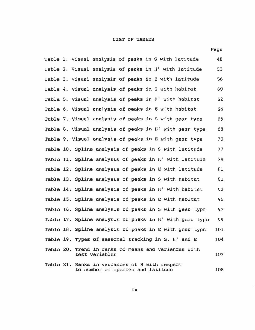
LIST OF TABLES

Page

Table 1. Visual analysis of peaks in S with latitude 48

Table 2. Visual analysis of peaks in H' with latitude 53

Table 3. Visual analysis of peaks in E with latitude 56

Table 4. Visual analysis of peaks in s with habitat 60

Table 5. Visual analysis of peaks in H' with habitat 62

Table 6. Visual analysis of peaks in E wlth habitat 64

Table 7. Visual analysis of peaks in s with gear type 65

Table 8. Visual analysis of peaks in H' with gear type 68

Table 9. Visual analysis of peaks in E with gear type 70

Table 10. Spline analysis of peaks in S with latitude 77

Table 11. Spline analysis of peaks in H' with latitude 79

Table 12. Spline analysis of peaks in E ~-~i th latitude 81

Table 13. Spline analysis of peaks in s with habitat 91

Table 14. Spline analysis of peaks in H' with habitat 93

Table 15. Spline analysis of peaks in E with habitat 95

Table 16. Spline analysis of peaks in s with gear type 97

Table 17. Spline analysis of peaks in H' with gear type 99

Table 18. Spline analysis of peaks in E with gear type 101

Table 19. Types of seasonal tracking in s, H' and E 104

Table 20. Trend in ranks of means and variances with test variables 107

Table 21. Ranks in variances o f S with respect to number of species and latitude 108

ix

LIST OF TABLES Continued

Page

Table 22. Ranks in variances of H' with respect to number of species and latitude 110

Table 23. Ranks in variances of E with respect to number of species and latitude 112

Table 24. Ranks in the means of S with respect to number of species and latitude 115

Table 25. Ranks in the means of H' with respect to number of species and latitude 117

Table 26. Ranks in the means of E with respect to number of species and latitude 119

Table 27. Summary of autocorrelation analysis of s 122

Table 28. Summary of autocorrelation analysis of H' 124

Table 29. Summary of autocorrelation analysis of E 126

Table 30. Data sets with 'smooth correlograms' in S, H' and E and test variables 129

Table 31. Data sets with 'spiky correlograms' in S, H' and E and test variables 130

•rable 32. Data sets with both 'smooth' and 'spiky' correlograms in S, H' and E and test variables 132

Table 33. Time lapse of prediction of pattern in S, H' and E for data sets with 'smooth correlograms' 133

X

LIST OF FIGURES

Figure 1. Geographical distribution of data sets

Figure 2. Comparison of dispersion of H' from simulated and real data

Figure 3. Comparison of dispersion of E from simulated and real data

Figure 4. Comparison of seasonal pattern of H' from simulated and real data

Figure 5. Comparison of seasonal pattern from simulated and real data

Figure 6. Visual analysis of peaks in s with latitude

Figure 7. Visual analysis of peaks in H' wlth latitude

Figure 8. Visual analysis of peaks in E with latitude

Figure 9. Spline analysis of peaks in S with latitude

Figure 10. Spline analysis of peaks in H' with latitude

Figure 11. Spline analysis of peaks in E with latitude

of

Figure 12. Regression of date of first peak S with latitude

Figure 13. Regression of date of first peak H' with latitude

Figure 14. Regression of date of first peak E with latitude

xi

E

in

i n

in

Page

37

40

42

44

50

55

58

72

71

76

84

86

88

1 INTRODUCTION

Seasonal patterns of diversity in animal communi ties

reflect changes in community structure with time. Temporal

variation in community structure results from changes in

species composition and their relative abundances in the

community over time. In trying to understand the structure of

communities and the patterns of change in the structure with

t.ime, ecologists have traditionally looked at measures of

diversity of communities to try to understand such change in

structure. Reviews by Pianka (1966), Peet (1974), and

Washington (1984) covered the developments in the concept of

diversity and the diversity indices that have been used to

measure diversity in communities of organisms. Pielou (1966)

described and classified types of biological collections one

can get by sampling any community. A key for the

classification of the type of collection and which index of

diversity is suitable for the collection was also presented.

Pielou (1969) and Magurran (1988) provide a good coverage of

indices of diversity which are in use and also discuss their

relc.tive merits.

Diversity measures have two components; the measure of

the variety and richness of communi ties is one whilst the

measure of the relative abundances of the different species in

communities is the other. Indices such as the total numbers of

species present, S, measures the former while indices such as

2

the Shannon-Wiener index of diversity H', attempts to measure

both (Peet, 1974; Magurran, 1988). Furthermore, indices such

as the species evenness index E, which 13 a ratio of observed

diversity H' , to the maximum diversity of the community ( Hm.•x),

where Hmax=ln S (Feet, 1974), are often used to measure the

relative magnitude of the two components of diversity

measured, compared to the maximum possible (Magurran, 1988).

That is, E measures the relative abundance of each species in

the community: an evenness value of 1.0 means all species arc

equally abundant. For the purposes of consistency and clarity

the terms "richness", "heterogeneity", and "L·.JUitability" will

be used throughout the text in association with the three

diversity indices; S, H' and E respectively. This terminology

follows that of Feet (1974).

Seasonal patterns of diversity in marine fish communi ties

are the primary interest of this thesis. If seasonal patterns

of variation in diversity can be discerned, then these should

be useful for purposes of predicting changes in community

structure. If seasonal patterns of div~rsi ty can be predicted,

this should be useful for applied purposes such as fisheries

management and aquatic ecosystems management. In pollution

management studies in aquatic ecosystems, fish data have been

used to assess pollution and habitat degradation (Bechtel and

Copeland, 1970; McErlean et al., 1973; Haedrich and Haedrich,

1974; Haedrich, 1975; Livingston, 1975; Hilman et f3.l . . , 1977;

3

Potter et ~~-~ 1986). In such studies, fish diversity

statistics are often used to describe seasonal patterns of

diversity and community structure.

It is important in environmental management problems such

as impact assessment that studie.s be appropriately designed to

solve the specific problem(s) in question. Because natural

variations within ecological systems can easily confound with

variations incurred by anthropogenic causes, i mproper designs

and irrelevant temporal and spatial scales selected for a

study can fail to detect impacts (Green, 1989). Stressing the

importance of proper design, Eberhardt and 'l'homas ( 1991)

stated that unlike controlled experimentation, ecological and

environmental research often do not meet the criteria of

modern experimental design. In impact assessment studies the

sampling design is often planned to accomplish two principal

goals (Underwood and Peterson , 1988). The first goal is to

formally detect and confirm that a change in the system has

occurred. Secondly, the sampling design should allow the

assessment of whether the observed change is due to the impact

(e.g. pollution) or whether it is due to some other natural

processes. To achieve the first goal often requires the

execution of pilot studies or the utilization of existing

baseline ecological data (Clarke and Green , 1988; Green ,

1989). In situations where such baseline data are unavailable

or financial resources for pilot studies are limited,

4

established pattex·ns in community structure can become usofu.l

in this respect.

In studying seasonal patterns of diversi t.y and community

structure, the choice of what temporal scales to use depends

on the nature of the problem being investigated and some

knowledge of the biology and ecology of the species concerned.

Quarterly and monthly time scales are commonly used in the

study of seasonal patterns of diversity and communi t:y

structure in fish communi ties. The finer resolutions of

seasonal patterns are only adequately shown over mont hly

intervals. This has been assessed quantitatively for ben t h i c

invertebrate and fish data (Livingston, 1987).

The existence of seasonal patterns in diversity in fish

communi ties is evident from various studies. Most of these

earlier studies which looked at seasonal patterns in diversity

and community structure in fish communi tir~s, have been on the

east coast of United States (Merriman and Warfe l , 191\8:

McFarland, 1963: Richards, 1963: Dahlberg and Odurn, 1970;

Tyler, 1971; Oviatt and Nixon, 1973; Haedrich and llaedrich,

1974; Subrahmanyam and Drake, 1975; Hilman ~..t a_],., 1977; Ho f f

and Ibara, 1977). Besides studies on the east coast o f the

United States other studies have been done in California

(Allen and Horn, 1975), Mexico (Warburton, 1978), Severn

Estuary (U.K. ) (Claridge e~ Q.l_., 1 CJ86), Sweden (Thorman,

1986), Australia (Quinn, 1980; Rainer, 1984), Kuwait (Wright,

5

1989), southern Iraq (Al-Daham and Yousif, 1990), and Cape

Coast, South Africa (Bennett, 1989).

Published studies have shown considerable seasonal change

in diversity. Species richness, which is measured in this

study by the index s, has been reported to vary seasonally by

severa 1 studies. It was generally reported to be low in colder

months and high during warmer months (McFarland, 1963;

Richards, 1963; Shuntov, 1971; Oviatt and Nixon, 1973; Hoff

and Ibara, 1977; Warburton, 1978; Quinn, 1980; Rainer, 1984;

Thorman, 1986). Variations do exist in terms of the specific

timing of the occurrence of these seasonal highs and lows in

species richness but not the general trend of more species in

warmer months and a decline in species richness in the colder

months. Studies by McFarland ( 1963) in Texas and Richards

( 1963) in New York, both showed that the richness component of

diversity was low in the winter months and high in the summer

months. Species .:-ichness was reported to be high in October

and low in January in a study in Narragansett Bay (Oviatt and

Nixon, 1973). Two more studies from the North American East

Coast, also reported species richness to reach a maximum in

the summer. These were reported from Florida ( Subrahmanyam and

Drake, 1975) and Massachusetts (Hoff and Ibara, 1977). This

s · ~asonal trend in species richness was also reported from

California (Allen and Horn, 1975; Allen, 1982) and Mexico

(Warburton, 1978). Further studies which rP.ported this pattern

6

in areas other than North America were in S\oJeden

(Thorman,1986); northern Australia (Shuntov, 1971; Quinn,

1980; Rainer, 1984); Kuwait (Wright, 1989) southern Iraq (A1-

Daham and Yousif, 1990); South Africa (Bennett, 1989). One

study reported a reverse seasonal pattern in species richness;

species richness was higher in the colder months. This was

shown by a study done in Severn Estuary, U.K. (Claridge et

al., 1986).

The seasonal pattern of the heterogeneity component of

diversity shO\'led that peaks occurred in either warm and cold

seasons of the year; usually one or the other occurred in any

one study. Maximum values in the heterogeneity component of

diversity in warmer months were reported by a number of

studies (Oviatt and Nixon, 1973; Subrahmanyam and Drake, 197 5;

Allen and Horn, 1975; Warburton, 1978; Al-Daham a nd Yousif,

1990). Other studies reported maximum values in this component

of diversity during the colder months (Hoff and Ibara, 1977;

Allen, 1982; Claridge et al., 1986).

The equi tabili ty component of diversity showed a seasonal

pattern similar to that for the heterogeneity component o f

diversity. That is, maximum values were observed i n both wurm

seasons (Dahlberg and Odum, 1970; Warburton, 1978; Al-Daham

and Yousif, 1990) as well as cold seasons o f the year

(Claridge et al., 1986).

The above studies indicate one pattern to be common. Tha t

'7

is the richness component of diversity reached maximum values

in the warmer months. This ranged from March to about October

in the northern hemisphere studies (McFarland, :1.963; Richards,

1963; Warburton, 1978; Thorman, 1986; Wright, 1989; Al-Daham

and Yousif,1990) and from December to March in the southern

hEmisphere studies (Quinn, 1980; Rainer, 1984; Bennett, 1989).

Late spring into early autumn is generally n=!garded as warm

months while late autumn to early spring can be generally

regarded as cold months, within an annual cycle. 'rhe specific

months for these warmer and colder coudi tions wilJ be

different in the two hemispheres hence this difference should

be borne in mind when referring to seasonal patterns reported

by seasons (i.e spring, summer, autumn and winter) . That is

the summer in the northern hemisphere is from about June to

late early September while in the southern hemisphere this

period is winter. Unlike species richness \-lhich appeared to

show a fairly consistent warm-cold trend, the heterogenei·ty

and equi tabili ty components of diversity seemed to show ei thor

pattern in different studies. This implies that all three

components of diversity can either track each other, o:r that

the heterogeneity and equi tabili ty components of diversity can

show an opposite seasonal pattern to that of species richness.

Whenever the peaks and troughs in the three diversity indices,

C' .... , H' and E, closely follow each other, this represents an

equitable influx and efflux of species. An equitable influx

8

occurs when S, H' and E increase toget!aer. If S shm'ls a peak

while H' and E decrease, this trend represents an inequitable

influx and efflux •::~f species due to one or two dominant

species. A schematic illustra·t.ion of the two types of tracking

of the three indices is given in Figure Al, Appendix A.

From the above descrip1:ions of seasonal variation l n

diversity, it .is evident tha·t seasonal patterns in diversity

do exist in fish c:ommunit:l~~s. Species distributions and

compositions, as well as environmental factors which are often

found to influence them, vary geographically. Thus, one asks

whether one can differentiate between general patterns (those

occurring over large geo£Jraphical scales) and thoso sppt..:ific

to particular 1:ypes of: fish communi ties (those occurring over

local scales). This question deals with large spatial scales

and can only be sufficiently addressed by a comparative

approach. If large scale patterns do exist, then this should

be useful in applied fields such as impact and pollution

assessment as well as fisheries management.

From this review of the literature on studies on seasonal

patterns of diversity and community structure of fish

communities, it is evident that although numerous small scale

or single study investigations on the subject have boen

published, no major large scale comparative studies have been

reported. One recent study used published data sets for fish

captures on power station intake screens from t\lml ve sites

9

throughout England and Wales to study the seasonal patterns of

diversity and community structure of inshore fish communi ties

(Henderson, 1989). This study demonstrated both temporal

( seasonal) as well as spatial (latitudinal) trends in

diversity and community structure. I aim to integrate both

local and large scale seasonal patterns of diver~i ty and

community structure of fish communi ties in this study , which

if accomplished, will be useful for applied purposes.

The information reviewed above can be summarized as a

working hypothesis that seasonal patterns in diversity in

marine fish communities exist, and these patterns are

regula ted by processes influenced by the interaction of a

range of biotic and abiotic variables operating in concert.

The principal objective of this study is to analyse this

hypothesis and propose further testable ones. The study will

specifically involve firstly, using published data sets to

discover seasonal patterns of diversity in marine fish

communi ties. Any apparent patterns discovered will be

described, to allow general seasonal patterns (patterns

occurring over large geographical scales) to be separated from

ones that are specific to local scales. These described

patterns will be used to propose further hypotheses about the

processes and mechanisms regulating seasonal patterns of

div,•rsi ty in marine fish communi ties. Finally, these seasonal

patterns, any relationships among the three components of

10

diversity { dchness, heterogenei 1:y I and equi tabi li ty ) I and the

proposed hypotheses will be used to .Ulustrate examples of hO\v

these information can be used by researchers in applied fields

that use diversity statis·tics de:r:ived from fish catch da ·t.a,

such as fisheries management and marine pollution, to design

and execute more sensitive tests.

To achieve these objectives I two analytical techniques

will be used to identify seasonal patterns of diversity. These

are: ( 1) a graphical technique: and ( 2) the use of statisticG

(means, variances and autocorrelation coefficients) of the

indices S, H' and E. The graphical technique will allow for ,,

visual display of any seasonal patterns as well as any

possible trends in these patterns. In the use of sample

statistics, the ranks of the means, variances, and the

autocorrelation functions o£ the time series of each index for

different data sets will be used. These ranks will he

analysed with respect to major explanatory variables such as

habitat type, type of gear, and latitude, within geographicn1

regions with similar climatic regimes, to determine whether

any relationships exist among the ranks of the differenl

statistics and the explanatory variables.

2 MATER:U\LS AND METHODS

2. 1 Data acquisition

Data used in this study were obtained through published

sources. Literature search for relevant publications was done

by using computer search methods, searching through the

contents of every volume of key journals, and following up

relevant references from every appropriate article. The key

journals searched were: Marine Biology; Bulletin of Marine

Science; Marine Ecology Progress Series; Estuarine Coastal and

Shelf Science; Estuaries; .Journal of the Marine Biological

Association of the United Kingdom; Journal of the Marine

Biological Association of India; Environmental Biology of

Fishes; Canadian Technical Reports of Fisheries and Aquatic

Sciences. Additional journals searched to some extent were:

Fishery Bulletin (U.S o ) ; Australian Journal of Marine and

Freshwater Research; Canadian Journal of Fisheries and Aquatic

Sciences; Journal of Fish Biology o

Throughout the search, the selection criteria for

articles were that: ( 1) the study should involve monthly or

fortnightly sampling for six months or more; ( 2) all data

presented should be sampled by a single sampling gear or where

more than one gear type is used, data from each type of gear

should be separable; ( 3) taxonomic information should be

complete to species level or if species are unidentified, they

should be distinguished from other related species and be

12

consistently recorded by a tentative identification; and ( 4)

the sampling procedures usert should be sufficiently and

accurately described to allow for the calculation of catch per

unit effort (CPUI::) statistics. Based on these criteria, a

total of 22 data sets were selected for this study.

Data sets were either obtained directly from the

publications whenever these were presented or were requested

from the authors. From an initial attempt of thirteen

requests, only one au·i:hor responded by sending orJginal data.

This poor response resulted in abandoning this method of

obtaining data. The twenty-two data sets used in this study

were largely compiled from published sources; they are

available for use upon request.

2.2 Data processing

All data sets acquired were stored as ASCI I files using

Memorial University's mainframe (VAX/VMS) computer. The data

sets were separated by sampling stations and by type of

sampling gear used. These data files \'lere the parent fj J es

from which subsequent manipulations and specific analyses \-tere

done.

2.3 Data analysis

Data analysis was done with three computer soft\-tare

packages. Graphical analyses were performed ~lith sIGMA PLOT

13

and MATHCAD. Statistical analyses were performed with MINITAB,

which was available on the University's mainframe computer.

Two analytical techniques were used in data analysis; the use

of graphical analysis was one technique and the use o£

statistics (means, variances and autocorrelation coefficients)

was the other.

Graphical methods are often useful in exploratory data

analysis as they display any patterns existing in the data.

This enables the researcher to extract visually any possible

relationships between the pattern in the data and the

variables concerned. It also allows the researcher to deci de

on appropriate methods of data analysis to use for testing

these relationships statistically.

The statistical technique used was the analysis of the

autocorrelation coefficients, and the ranks of the means and

variances of S, H' and E. These statistics were analysed with

respect to a number of explanatory variables. Habitat type,

gear type, and latitude within major geographical regions

grouped according to similarities in climatic patterns, t·tr:re

the main explanatory variables used. The ranks of means and

variances for each indt:~:x were checked against each of the

explanatory variables to uncover any rel ationships that

existed. Similarly, the autocorrelation coefficients of the

three indices of diversity were analysed by testing the types

of correlograms of different data sets with the explanatory

14

variables for any relationships.

Several major ~ndices of d~ versi ty are available and

their descriptions and merits have been discussed in a number

of publications (Pielou, 1969; Legendre and Legendre, 1983;

Washington, 1984; 1'-lagurran, 1988). Statistical properties of

these major indices have been compared using data from n

copepod community by Heip and Engels (1974). They showed that

the Shannon-Wiener index H' , was the index that gave a better

measure of the diversity of the copepod community in terms of

the variability and conformity of values calculated for

individual samples and that of all samples pooled. No

consensus exists as to which indices are better and which a r e

not (Washington, 1984; Magurran, 1988). Besides this lack of

consensus, there are also limitations to the biologicn l

interpretations among values of the different diversty

indices. This is because many indices are ratios of meaning£ul

biological variables such as species richness and relat i ve

abundance, and therefore share information (Poole , 1974). Tho

problem arises when these two types of information about a

community are compounded into a single numerical meosurc

(Poole, 1974) as in the Shannon-Wiener index H'. Many such

indices are in use today (Washington, 1984; Magurran, 1988) .

To guard against this problem one must carefully consider the

suitability of sampling methods and designs planned for

collecting species diversity data from a particular commun i ty

15

(Green, 1979), and selecL op~ropriate indices for the samples

collected respectively (Pielou, 1966; Poole, 1974).

Despite this limitation, paying critical attention to

sampling and statistical aspects of selected indices can give

information about the biology of the system studied. This has

been shown with data from bird, benthos and plankton

communities (Webb, 1974). My reasons for using the above

indices are as follows. (1) Species richness that is measured

by the index S, is based on the total counts of the number of

species in a collection. It is an absolute and fundamental

measure of specie~ diversity (Magurran, 1988) since it

measures directly the species content of a sample. (2) The

Shannon-Wiener index has been widely used in diversity studies

in fish communi ties and so it is used here to enable

comparisons of seasonal patterns of this index in this study

with previous ones if necessary. (3) The Shannon-Wiener index

combines both the number of species present in the sample as

well as the apportionment of the number of individuals into

the different species ( Peet, 1974; Magurran, 1988). ( 4) A

common observation in animal and plant communi ties is that

often most individuals in a community belong to a small number

of dominant species while a large number of species are

represented by a small number of individuals (Margalef , 1958;

Hughes, 1986; Lawton, 1990). This generally means that the

number of individuals per species in most animal and plant

16

communities tend to be a logarithmic function of the rank in

abundance of the constituent species of the community.

According to information theory (Shannon and Weaver, 1949) the

Shannon-Wiener index H • , has properties that approxima to

properties of theoretical models of species distribution such

as the log series and log-normal distributions. Therefore, the

Shannon-Wiener index is chosen for use in this study. (5) The

evenness index E, which measures the equi tabili ty component of

diversity, is also selected because it is a measure of the

ratio of the heterogeneity H 1 of the sample to the maximum

heterogeneity possible if all the species were equally

represented ( Peet, 1974; Magurran, 1988). 'l'herefore, this

index gives us a handle on whether or not the species in the

community from which the samples were obtained, are

numerically equally represented. (6) Because each of the three

indices looks at a different aspect of diversity, they were

all used here in order to describe the overall structure of

the community.

2.3.1 Calculation of diversity indices

The diversity indices calculated were: the total number

of species S, recorded for a station on each sampling dote;

the Shannon-Wiener index of diversity H 1; the species ovormm:~s

index of diversity E. The formulae for these indices were as

follo~.o.$:

17

s total number of species recorded at a site on a

sampling date;

HI (Equation 1)

where p 1 = the proportion of the ith species in the

sample ( p1 = nJN):

n 1 is the total number of individuals of the ith species;

N is the total number of individuals of all species in

the sample.

E = H 1 /ln s (Equation 2)

where ln S is equal to the maximum diversity ( Hmax) of the

community (Feet, 1974).

H1 and E were both calculated using the MINITAB statistical

package. Computation routines saved as macros (a saved set of

executable MINITAB commands) were executed sequentially to

obtain each ~ndex for each data set.

The sequence of the computations to obtain H 1 was as

follows: (1) the proportion of each species (p1 , p 2 , ••• p 1 ) for

each sampling date was calculated; (2) the natural logarithm

(ln) of each p was calc11lated and stored; (3) the product of

the values in (1) and (2) respectively were then computed,

18

giving a value corresponding to each species for each sampling

date in the data set; and (4) summing up the values obtained

in (J) for each sampling date finally gave the respective H'

values (see equation 1}.

To calculate the species evenness values E, for each

sampling date, the natural logarithm of the number of species

S, for each date was co~puted. This was then divided into the

corresponding value of H' obtained in (4) above, to give the

respective evenness value (see equation 2). All values of s,

H' and E for each sampling date for each study were then saved

for the subsequent analyses of seasonal patterns.

2.3.2 Effect of sampling bias on seasonal patterns

In any sampling programme, regardless of the type of gear

used, the catchabili ty of the gear varies for different

species as a result of factors such as gear efficiency,

distributional patterns of the different species, and their

response to the gear (Taylor, 1953; Kenchi ngton, 1980; Byrne

et al., 1981; Gulland, 1983). Catchabllity is conventionally

designated as q in the fisheries literature, and is also

termed a "catchability coefficient" (Rickel, 1975; Kjelson and

Johnson, 1978; Gulland, 1983; Blaber ~.t 9!., 1990}. This

coefficient q, in the instance of trawling gear, is defined as

the ratio of individuals of a certain species caught by the

trawl to the total number of that species in the path of the

trawl (Ricker, 1975; Kjelson and Johnson,

19

1978).

Mathematically, this relationship can be repreGanted by the

equation:

q = c/n (Equation 3)

where q = the proportion of individuals of a species in

the path of the gear, represented in the catch;

c = the number of individuals of a species in the catch;

n = the total number of individuals of a species in the

path of the gear.

This study used catch data obtained from published

studies. All data sets used in this study used a single gear

type, except one (Allen, 1982), which was collected by

multiple gear types. This data set was accepted for use in

this study because a common effort was possible to calculate

for the different methods used, enabling the standardization

of the catch in terms of this common effort. It was important

to observe the above criteria in compiling the data sets

because the catchability of different gears for different

species differ and never have a perfect catchability of q =

1.0 (Taylor, 1953; Kenchington; 1980; Byrne et al., 1981;

Gulland, 1983). Therefore, it was important to determine

whether keeping any imperfect catchabilities in gear (q < 1.0)

20

for the different species constant, among samples within a

study, would give comparable seasonal patterns for H' and E to

those discerned under situations of perfect catchability (q =

1.0) for all species. If the two patterns are the same, then

one can assume that as long as the sampling design and the

sampling programme were constant within a study, the seasonal

patterns discerned from the catch data are not biased by

differential catchability of species.

To assess the above question, the data set of Macdonald

et al. (1984) (see Tables Bl and 82, Appendix B) was

arbitrarily chosen to analyse whether imperfect catchability

affected the interpretation of the seasonal patterns observed;

q = 1.0 would imply that c = n. From the catch (c) in this

data set 300 data sets were simulated, each to represent

possible total numbers (n) for each species exposed to tho

gear. In each simulation different values of q were randomly

generated for each species in the data set. Within each

simulation these values of q were kept constant for each

species. This simulation procedure was as follows: (1) MINITAB

was used to generate random values between 0.2 and 1.0 for q

from a uniform probability distribution for each species in

the data set; (2) the catch c, in the original data set for

each species was divided by the corresponding ~.i ~;o give a

simulated data set which represented the simulated n for oach

species (see equation 3); (3) H' and E for this simulated data

21

set were then calculated following the computational sequence

for calculating the two indices described in 2.3.1 above; and

(4) the values for H' and E were then saved. This routine was

repeated 300 times.

The 300 values of H' and E were then giaphically

analysed. This was done to see if the seasonal pattern of

diversity from the original data set differed significantly

from that for the 300 data sets simulated with constant

randomly generated catchabili ties for each species, throughout

all sampling dates. To assess the dispersion of the values of

both H' and E calculated for each sampling date from the

simulated data sets, "Box and Whiskers" plots were done for

each index . . These were plots of the quartiles of the

distribution of the 300 values for each index for each

sampling date. The values for H' and E calculated from the

original data set were then superimposed on the "Box and

Whiskers" plot. This was done to display the variability in

the values of each index from the 300 simulated data sets, in

relation to the corresponding values of the two indices from

the original data set. Values of H' and E of the original data

for each sampling date were further compared with the values

of the two indices obtained from data from two of the 300

simulations. This was done by comparing the graphs of H' and

E calculated from the original data and the values of the two

indices calculated from data from two of the three hundred

22

simulations. The twd simulations used for the comparison were

arbitrarily chosen. From this comparison, it was determined

whether the seasonal pattern of diversity changed when n was

varied at each simulation by a new set of random

catchabilities for each species.

2.3.3 Approximate randomization test

A randomization test was used to determine whether H' and

E calculated from these simulated values of n differed

significantly from the values of the two indices calculat~d

from the original catch (c) data. The simulated data sets were

obtained by randomly generated catchabilities as described in

2.3.2 above. This procedure is called an "approximate

randomization test" (Noreen, 1989). It involves randomly

generating samples from a pool of all possible values of a

variable which are obtainable by complete permutation and then

calculating the required statistic from these samples. In this

case n was the variable sampled and H' and E were the required

statistics. For each simulated data set obtained from randomly

generated catchabilities, H' and E were calculated by

executing macros that carried out the computations described

in 2.3.1 above. The values of the two indices corresponding to

each simulation were saved together. To compute the

descriptive statistics for the 300 sets of values for H' and

E which were obtained from simulated values of n, it was

23

necessary to separate each set of values for each index from

the 300 files in which they were stored. The 300 files

containing H' and E from each simulation were retrieved in

batches of fifty files at a time into MINITAB and the values

for H' and E were then resaved separately. Fifty files were

sorted at a time by repeatedly executing a macro which

conveniently did the sorting because randomization methods are

often lengthy and time con·:;uming. Repeating this procedure six

times resulted in six such files each for H' and E, all with

a data matrix of fifty columns (corresponding to fifty

s .~mulations of random catchabili ty) X sixteen rows

(corresponding to sixteen sampling dates). Finally, these six

files for H' and E respectively, were combined to give the

final 300 x 16 matrix for each index. The descriptive

statistics for the 300 values for each index for each date

obtained from the simulated data sets were calculated from

these two final matrices. These descriptive statistics were

then used to analyse and compare the dispersion of the 300

values of H' and E for the simulated data sets with respect to

the values for each index for the original data set.

2.3.4 Analysis of seasonal patterns of diversity from sigma­

plot graphs

Graphical analysi~ for seasonal patterns in s, H' and E

was done using SIGMA PLOT. Visual inspection of these graphs

24

was done to identify major peaks and troughs and to look for

general seasonal patterns in the three diversity indices.

Those plots of S, H' and E, were all plotted onto a single

page, each index with a suitable y-axis and all indices with

a common x-axis. Exact dates were plo~ted, 01 where such was

not possible from the data, Julian dates corresponding to the

middle of each month were used. This arrangemen~ of graphs

allowed for simultaneous comparisons of seasonal patterns in

the three indices.

2.3.5 Visual analysis of sigma-plot graphs

The graphs drawn with SIGMA PLOT were ordered by latitude

within four major geographical regions from which the data

sets were collected. The four regions were: (1) Europe; (2)

North American East Coast; (3) Mediterranean, South Africa,

and North American West Coast; and (4) Tropics/Subtropics.

Marine biogeographic regions mapped according to the

distributional patterns of shore and shallow sea fauna

(Hedgpeth, 1957) were used to group the above regions.

Hedgpeth's biogeographic regions were based on littoral

provinces of the world classified by Ekman (Ekman, 1953 op

cit. Hedgpeth, 1957). Those provinces were: Arctic-Antarctic;

Boreal-Antiboreal; Warm Temperate; Tropic. They reflected

temperature regimes associated with latitude. According to

this scheme, the appropriate biogeographic provinces for the

25

respective regions were: Europe - Boreal; North American East

Coast - Arctic, Boreal, Temperate; Mediterranean, South Africa

and North American West Coast Warm Temperate,

Boreal/Antiboreal; Tropics/Subtropics - Tropic. Within each

region the data sets were ordered latitudinally from north to

south and the seasonal patterns of S, H' and E from data sets

from the respective regions were inspected for patterns with

the various explanatory variables. The main explanatory

variables were latitude, habitat type and gear type.

To carry out the analysis, a form was drawn up to record

the location of each study, position (latitude/longitude) and

months of sampling. By visual inspection each major cycle of

increase and decrease in each index, S, H' and E, was

identified. Months of highest and lowest values of each index

in each major cycle were then recorded on the form. This

information on the timing of the peaks and troughs of each

index were then plotted. To ensure consistency in the

analysis, definitions for 'peak' and 'trough' were necessary.

A 'peak' is defined here as the highest point which is

approached by a series of progressively increasing data points

and departed from it by a series of progressively decreasing

points, in a time series plot of any of the three indices. A

change within either an overall increasing or decreasing trend

by a minimum of one data point was not considered a change in

the general trend. A 'trough' is defined as the lowest point

26

between any two adjacent peaks in a time series plot of any of

the three indices. Peaks and troughs as defined here are

graphically illustrated in Figure A2 (Appendix A). These

definitions excluded any peaks and troughs at the start and

end of any time series in the analysis because those were

often not represented in a complete cycle.

Graphs of all data sets

regions were latitudinally

from the three geographical

ordered and each index was

separately plotted. Visual inspections of these plots enabled

comparison of major seasonal as well as latitudinal patterns

in each index within each of the major geographical areas.

Patterns related to possible influence of sampling gear and

type of habitat were also explored.

2.3.6 Spline analysis of seasonal patterns in S, H' and E

Spline analysis for the diversity indices S, H' and E, of

all data sets were done with the MathCAD software package.

This method was also used besides the visual method because it

is more quantitative and explicit. That is, different people

using the technique would obtain similar results for any data

set. On the other hand, the visual method may give slightly

different results in this respect, it has the advantage of

permitting intelligent judgements about ·outliers' in the

data, allowing one to appropriately plot seasonal trends in

the data. Spline analysis works best when serial data are

27

collected at equal intervals of time or space. Splines were

found to be highly sensitive to serial data collected at

unequal intervals. Hence, using both methods serves to cross

check the methods of analysis and their results.

The spline analysis involved fi t"ting linear splines

between knots. A spl".ne is a line of best-fit through the data

points within a pre-determined interval (i.e. the resolution)

while a "knot' in a spline plot is an imaginary line

perpendicular to the x-axis, the time axis in this case, that

marks the point at which splines on either side of it are

connected. When adjacent lines are connected at successive

knots, an overall line or a curve results; whether this spline

is straight or curved depends on the power of the function

that describes the relationship between the two variables

plotted. Detailed descriptions and examples of spline analysis

is given in Wold (1974). Figure A2 (Appendix A) shows plots of

both visual and spline analysis with respect to the original

data, for the time series for each of the three indices.

The resolution (i.e. the interval between successive

knots) in my analysis was pre-determined to span two data

points, giving resolutions of: sixty days on average for all

data sets collected over monthly intervals; thirty days on

average for those collected at variable time intervals that

ranged between weekly to monthly intervals; and fifteen days

for data sets collected at a weekly time interval or less. The

28

average resolution in each data set was computed using tho

formula:

(Equation 4)

where Rm is the resolution at knot m;

k is the number of data points spanned (2);

t 1 is time at sampling in Julian days of the ith sample;

t 1 is time at sampling in Julian days of the first

sample;

n is the sample size.

Using the above formula: seventeen data sets har.1 i::i resol u t.lon

of sixty days on average; four data sets had a resolution of

thirty days; and one data set had a resolution of fifteen

days, in the spline analysis for each index in the datn sets.

The analysis resulted in spline plots at appropriately

selected resolutions for each imlex in each data set. 'I'he

peaks and troughs were analysed in the same manner as was done

in section 2.3.5, according to their respective definitions.

For plots of each index of all data sets, the months and

corresponding Julian dates for each peak and trough in the

time series were tabulated. This data was compared with

latitude, habitat type and sampling gear, to determine any

relationships in the peaks and troughs with these v~riables.

29

2.3.7 Patterns of seasonal tracking of S with H' and E

In order to determine the differences in the type of

seasonal patterns ?f species richness S, the heterogeneity

index H' and the equitability index E in different data sets,

the major peaks and troughs visible from the original sigma­

plot graphs of each index for each data set were used. The

peaks and troughs of each index for each dn ta set were

examined to display the pattern of tracking of H' and E with

respect to the peaks in and troughs in species richness, S.

'fhe major pattern( s) of tracking in each data set observed

from this analysis were tabulated.

2.3.8 Ranks of variances and means of S, H' and E

Variances and means of the three diversity indices within

each of the data sets were analysed by ranking and checking to

see whether these statistics were relc.. ted to any of the

variables used in the analysis. Using MINITAB, ~he variances

and the means of S, H' and E of each study were calculated.

The means and variances for each index for each data set were

then ranked and tabulated separately, resulting in two sets of

tables. One set was for the variances of each index while the

other was for the means. In each set of tables, the type of

habitat for each study; latitude for each study; the total

n~rnber of species recorded in the data; the type of sampling

gear( s) used; the sampling interval; and the duration of

30

sampling, were recorded. These tables were then used to

determine whether the ranks in the variances and means for

each index in each data set showHd any relationships with any

of the variables listed above. For example, was high variance

in species number associated with a particular habitat, such

as the nearshore?

The variables that appeared to be related on a rank scala

to the three indices were then analysed in more detail. Hanks

of the variances and means of S, H' and E were also examined

in relation to latitude and the total number of species in the

data sets, to further describe the pattern with respect t:o

these variables.

2.3.9 Autocorrelation analysis of S, H' and E

Autocorrelation functions measure the correlation of any

pair of observations that are k lags apart (Montgomery and

Johnson, 1976) in a series of time-oriented observations

(Montgomery, 1991), called a time series (Montgomery and

Johnson, 1976). The seasonal values c.. ..: diversity .i nd i ces

analysed in this study is an example of such a series.

Autocorrelation coefficients, also called serial correlation

coefficients (Poole, 1974), measure the relative s trength of

association of pairs of observations formed by the original

time series sliding by one observation each time be s i de a copy

of itself (Platt and Denman, 1975) until the lag k,,_1 is

31

reached. Generally, when observations k lags apart have values

of similar magnitudes their autocorrelation coefficients will

be close to 1.0, while those with a large value succeeded by

a small value results in the coefficient having a value close

to -1.0. However, if such observations have very little

relationship, the coefficient would be approximately zero

(Montgomery and Johnson, 1976).

The formula for the autocorrelation functions according

to Legendre and Legendre (1983) is:

( Equation 5 )

= autocovariance at k I variance at zero lag~

k is the lag ( k 1 •••••• kn-t ) ~

rvv< k) is the autocorrelation coefficients at k and

ranges between -1 and +1. The signs indicate the

direction of the relationship.

Autocorrelation functions for the values of each index in each

data set were calculated with the MINITAB statistical package

by executing the autocorrelation function command.

Autocorrelation coefficients for the first lag and the highest

value for each series, for S, H' and E for all data sets, Nere

tabulated. Five explanatory variables which included latitude,

habitat type, type of gear used, the resolution of the time

32

series for each index, and the duration of sampling, were also

included in the table. Besides computing autocorrelation

coefficients for each lag of each series, MINITAB also plotted

correlograms of the computed values.

A correlogram is a plot of the values of the

autocorrelation coefficients versus lags in the series (Poole,

1974; Box and Jenkins, 1976; Legendre and Legendre, 1983).

When the oscillations in a correlogram rapidly dampens to zero

as k increases, this indicates that the oscillations in the

indices with time are not occurring in a "regular and

periodic" manner (Poole, 1974). If they are sinusoidal this

indicates that a regular periodic phenomenon exists

(Stephenson, 1978) .

Th~ee main patterns in correlograms for S, H' and E were

identified. A ' sinusoidal pattern' with each successi ve

coefficient being sequentially related both by rnagn i tude and

direction, was the first kind. In this pattern, connecting the

sequence of coefficients resulted in a sinusoidal curve. The

second pattern was one with each successive coefficients being

generally of a similar magnitude, and with a constant

direction. This pattern resulted in a 'uniformly 1 incnr

pattern' when each coefficient in the sequence was connected.

For the purposes of testing for relationships of these two

patterns ~n the correlograms with the five variables listed

above, they were classified together as ·smooth pattern'.

33

Thirdly, there was the type with the magnitude and direction

of the coefficients being highly variable, giving a ·spiky

pattern' . That is, a plot of the coefficients in the

correlogram appeared as spikes projecting in an irregular

manner either in a positive or negative direction in relation

to lags plotted on the x-axis.

The correlograms of S, H' and E for each data set were

inspected to determine the type of pattern as well as to

classify whether the autocorrelation pattern was ·smooth' or

·spiky 1 • Subsequently, the appropriate pattern of

autocorrelation for each index for each data set was recorded

with each of the five explanatory variables. For the purposes

of clarity in reporting these results, particularly when not

all indices of a data set were classified together under one

or the other of the two classes of autocorrelation patterns,

the data sets were divided into three categories. The first

category was ·all indices with smooth correlograms 1 • This

category contained all the data sets in which the correlograms

for all three indices had a ·smooth pattern 1 • Secondly 1 there

was the category 1 ·all indices with spiky correlograms 1 • It

contained the data sets whose c.;nrrelograms for all three

indices had a ·spiky pattern'. The third one was the 'mixed'

ca1:P.'1ory; it contained data sets with one or two of the three

indiceE belonging to either the first or second category.

A ·smooth correlogram 1 for any index means that the index

34

is correlated with a series of previous values. The sinusoidal

pattern that is characteristic of "smooth correlograms'

indicates that there is strong seasonality in the indices

(Stephenson, 1978). 'Spiky correlograms' indicate that the

values of the index concerned are correlated with few of the

previous values. This implies little or no seasonality in the

index.

3 RESULTS

3.1 Data sets compiled for this study

All suitable data sets acquired for this study are listed

in Table Bl and Table 82 (Appendix B). The ordering in the two

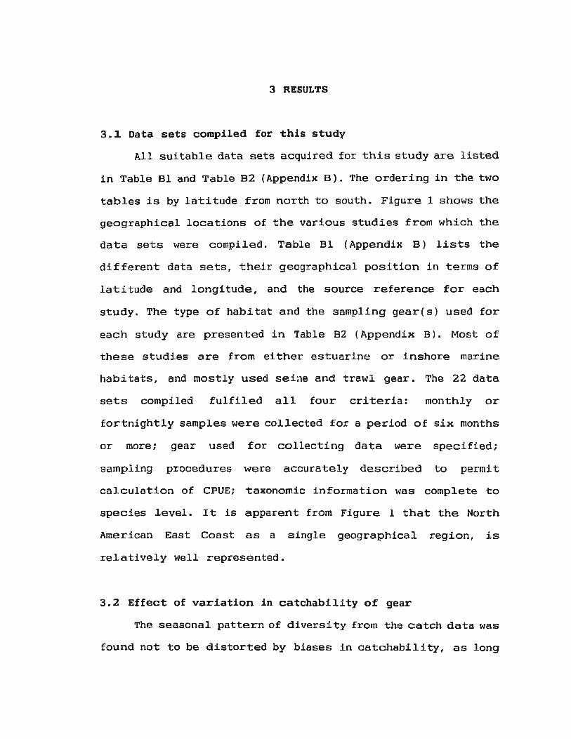
tables is by latitude from north to south. Figure 1 shows the

geographical locations of the various studies from which the

data sets were compiled. Table Bl (Appendix B) lists the

different data sets, their geographical position in terms of

latitude and longitude, and the source reference for each

study. The type of habitat and the sampling gear(s) used for

each study are presented in Table B2 (Appendix B) • Most of

these studies are from either estuarine or inshore marine

habitats, and mostly used seine and trawl gear. The 22 data

sets compiled fulfiled all four criteria: monthly or

fortnightly samples were collected for a period of six months

or more; gear used for collecting data were specified;

sampling procedures were accurately described to permit

calculation of CPUE; taxonomic information was complete to

species level. It is apparent from Figure 1 that the North

American East Coast as a single geographical region, is

relatively well represented.

3. 2 Effect of variation in catchabili ty of gear

The seasonal pattern of diversity from the catch data was

found not to be distorted by biases in catchabili ty, as long

Figure 1. Geographical distribution of data sets compiled

from the literature for this study. 'i'he numbers

representing the different data set correspond to

the numbers given in Tables 81 and 82 (Appendix 8).

=

= en

= CIO -

= en

38

as the b.ias was constant within study. The dispersion of 300

values for the Shannon-Wiener index of diversity H' , and the

species evenness index E, calculated from JOO data sets

simulated with randomly generated catchabili ty coefficients q ,

were plotted in Figure 2 and Figure 3, respectively. /\11 the

values for the two indices representing the original data fel l

within ·the middle boxes that encompassed 26%-75% of the values

in the respective frequency distributions for each 300

simulation for each sampling date. Most of those values for

the original data in both figures were very close to the

median.

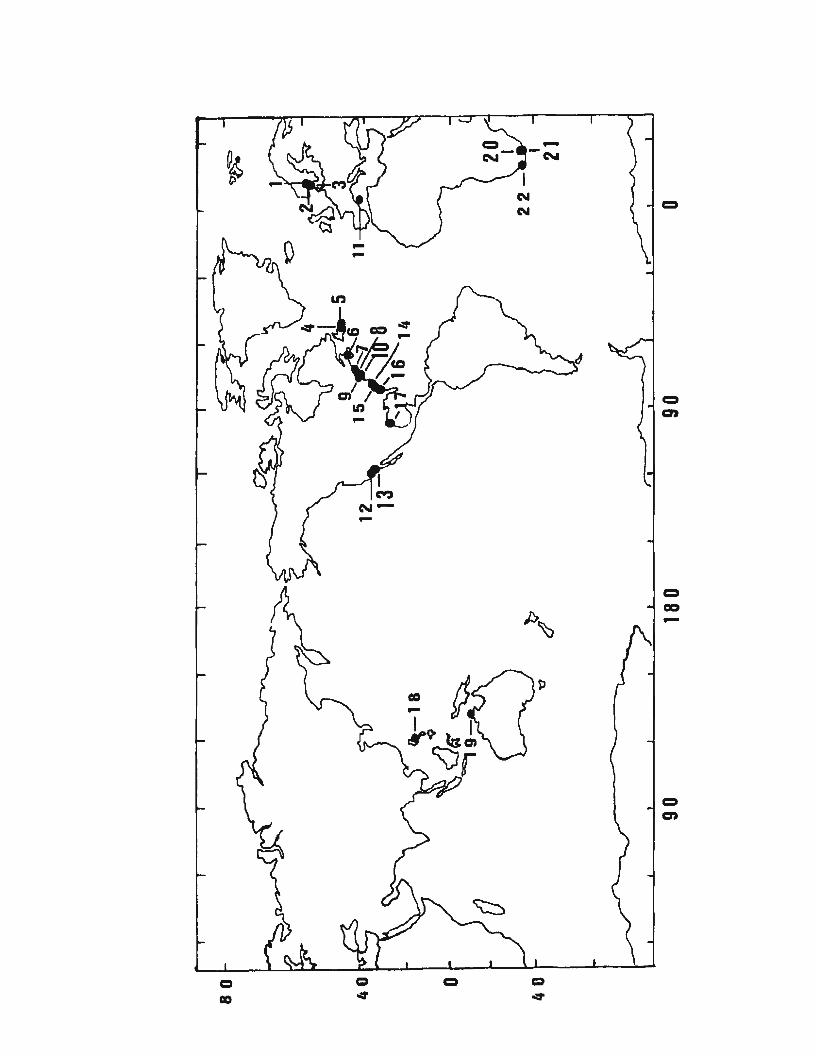
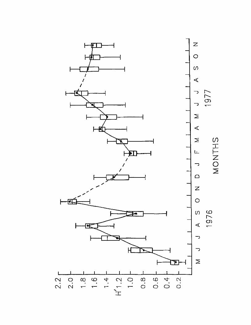
The seasonal pattern for H' and E are shown in Figure 4

and Figure 5 1 respectively. These figures compare the seasonal

pattern for each index calculated from the original data of

Macdonald et al. ( 1984) with those of two of the 300

simulations. From the comparison of the two graphs i t was

apparent that the seasonal patterns of H' and E in the catch

data did not differ from that of the two simulations.

3. 3 Visual analysis of graphs of seasonal patterns in S, H'

and E

Visual analysis of sigma-plot graphs of the three i ndices

showed general seasonal and latitudinal patterns to exls t in

fish communi ties. These seasonal patterns were more apparent

for the North American East Coast; a geographical region that

Figure 2. Graph for H 1 calculated from the original data

(Macdonald §:t. al., 19 84) • • ) and "Box and

Whiskers" plots ( r--cc::t-t) representing quartiles

for the dispersion of 300 values of H 1 calculated

for each month from data simulated with a constant

catchability for each species. The dashed lines (-­

- - -) indicate no monthly samples being taken.

z

0

(/)

I I <(

I

J f'. f'. (J") --, ~

2

<(

2 (/)

I LL 1-

I z I """") 0

I 2 1--P I. J 0

, ; z

0

(f) (.()

"' 01 <( ~

"""")

"""")

~

N 0 OJ C.O ~ C\1 0 OJ tO ~ N . . . . . . . . . . NN,-~,-~ ..- 0 0 0 0

' I

Figure 3. Graph for E calculated from the original data

(Macdonald et al. , 1984 ) ( • • ) and "Box and

Whiskers" plots ( t--CD--1) representing quartiles

for the dispersion of 300 values of E calculated

for each month from data simulated with a constant

catchability for each species. The dashed lines

( -----) indicate no monthly samples being taken.

z

0

(/)

I I <(

I

J r----. r----. 0)

J ..--

2

<(

2 (/)

I LL }-

J z

' 0 ' I T• • 0 ~ /

/ z / /

/

0

(/) tO ('... 0)

<( ..--

J

J

L

L_

0 CJ) OC) r---- c.o lf) ~ n N ~

• . . . . . . . . • ,....- 0 0 0 0 0 0 0 0 0

w

Figure 4. Seasonal pattern of H' versus time (months) for H'

of original data (Macdonald et al., 1984) and for

H' of two other of the 300 simulations. The two

simulations used for the comparison were

arbitrarily chosen; the comparision was done to

show that the seasonal pattern of H' from simulated

data is comparable to that of the original data.

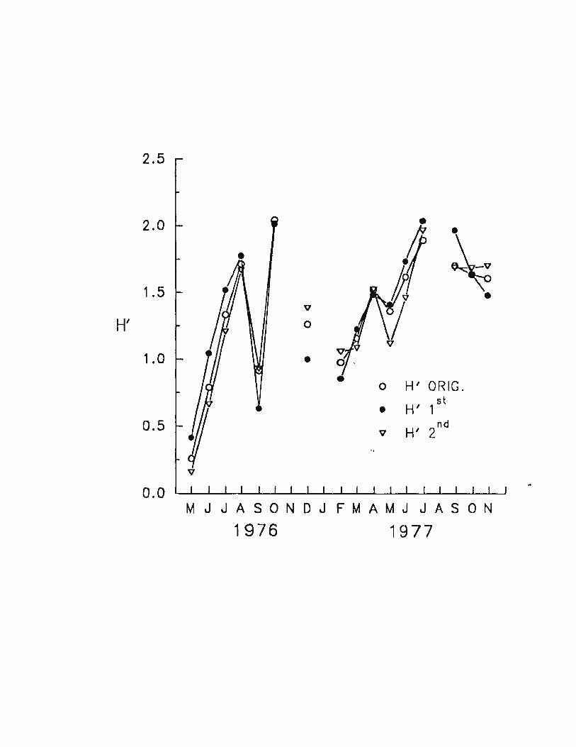
2.5

2.0 • • ~ 1.5 •

v

H' 0

1 .0 • • H' ORIG. 0

• H' 1 st

0.5 v H' 2nd

v

0.0 M J J A S 0 N D J F M A M J J A S 0 N

1976 1977

Figure 5. Seasonal pattern of E versus time (months) for E of

original data (Macdonald et §!., 1984) and forE of

two other of the 300 simulations. The two

simulations used for the comparison were

arbitrarily chosen; the comparison was done to show

that the seasonal pattern of E from simulated data

is comparable to that of the original data.

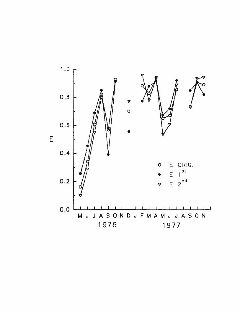
1 . 0

0.8 v • v

0

0.6 •

E

0.4

0 E ORIG.

• E 1 st

0.2 v E 2nd

0.0 I I I I I

M J J A S 0 N D J F M A M J J A S 0 N 1976 1977

47

is relatively well represented in terms of data sets, in this

study. A total of eleven data sets represented this region.

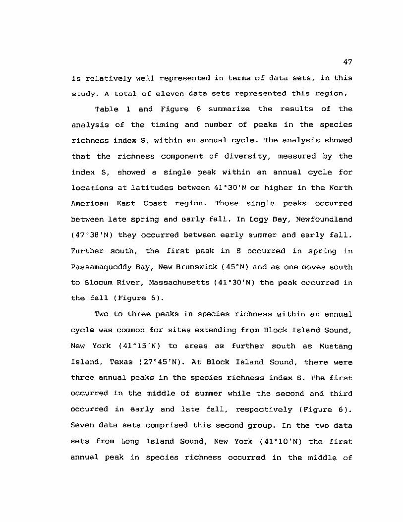
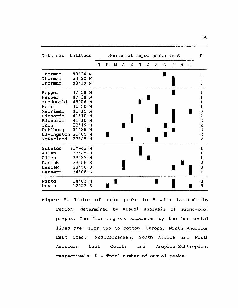
Table 1 and Figure 6 summarize the results of the

analysis of the timing and number of peaks in the species

richness index S, within an annual cycle. The analysis showed

that the richness component of divers! ty, measured by the

index S, showed a single peak within an annual cycle for

locations at latitudes between 41°30'N or higher in the North

American East Coast region. Those single peaks occurred

between late spring and Barly fall. In Logy Bay, Newfoundland

(47 °38'N) they occurred between early summer and early fall.

Further south, the first peak in S occurred in spring in

Passamaquoddy Bay, New Brunswick (45°N) and as one moves south

to Slocum River, Massachusetts (41°30'N) the peak occurred in

the fall (Figure 6).

Two to three peaks in species richness within an annual

cycle was common for sites extending from Block Island Sound,

New York ( 41 o 15 'N) to areas as further south as Mustang

Island, Texas (27°45'N). At Block Island Sound, there were

three annual peaks in the species richness index s. The first

occurred in the middle of summer while the second and third

occurred in early and late fall, respectively (Figure 6}.

Seven data sets comprised this second group. In the two data

sets from Long Island Sound, New York (41°10'N) the first

annual peak in species richness occurred in the middle of

40

Table 1. Numbers and Julian dates of major peaks in the

index S, determined by visual analysis of sigma­

plot graphs. The peaks are class i fied by lati t ude

and major geographical regionB: (1) Europe: (2)

North American East Coast; (3) Mediterranean,

South Africa, and North American West Coast; (4 )

Tropics/Subtropics.

Data set Latitude Region

1. Thorman 58°24'N 1

2. Thorman 58°22 ' N 1

3. Thorman 58°l9'N 1

4. Pepper 47 °38 ' N 2

5. Pepper 47°38'N 2

6. Macdonald 45°06'N 2

7. Hoff 41o30'N 2

8. Merriman 41°15'N 2

9. Ri chards 41°l0'N 2

10. Richards 41°10'N 2

11. Cain 33°19'N 2

12. Dahlberg 3l 0 35 ' N 2

13. Livingston 30°00'N 2

Julian day of pea k

1 2 3

258

289

289

2 96

192

165

228

225 304 3 52

147 289

147 28 9

99 247

136 289

45 258

'l'o t a J

# of

peaks

1

1

1

1

1

1

1

3

2

2

2

2

2

49

Table 1. Continued.

14. McFarland 27°45'N 2 145 238 2

15. Sebates 4l 0 -42°N 3 166 1

16. Allen 33°45'N 3 166 1

17. Allen 33o37'N 3 197 1

18. Lasiak 33°56'5 3 105 319 2

19. Lasiak 33°56'5 3 105 289 350 3

20 . Bennett 34°08'5 3 350 1

21. Pinto l4°03'N 4 75 228 258 3

22. Davis 12°22'5 4 50 280 355 3

Data set Latitude

Thorman Thorman Thorman

Pepper Pepper Macdonald Hoff Merriman Richards Richards Cain Dahlberg Livingston McFarland

Sebates Allen Allen Lasiak Lasiak Bennett

Pinto Davis

58°24'N 58°22'N 58°l9'N

47.38'N 47°38'N 45°06'N 41"30'N 41"15'N 41"10'N 41"10'N 33"19'N 31"35'N 30"00'N 27"45'N

4Qn-42"N 33"45'N 33"37'N 33"56'8 33"56'8 34"08'8

14"03'N 12"22'8

Months of major peaks in S

J F M A M J J A S 0 N 0

I I

I I

I I

I

I I

I

I I

I

I

I

I

I

I

I I

I I

I

I I

I I I

p

1 1 1

so

1 1 1 1 3 2 2 2 7. 2 2

1 l L 2 3 1

3 3

Figure 6. Timing of major peaks in S with latitude by

region, determined by visual analysis of sigma-plot

graphs. The four regions separated by the horizon taJ

lines are, from top to bottom: Europe; North American

East Coast; Mediterranean, South Africa and North

American West Coast; and Tropics/Subtropics,

respectively. P = Total number of annual peaks.

51

spring and the second occurred in early fall. Similar peaks

for the data set from North Inlet, South Carolina (33°19'N)

occurred a little earlier; the first in early spring and the

second in late summer. The fifth data set in this second group

was from Sapelo Sound and St. Catherine's Sound, Georgia

(31"35' N) where the species richness peaked in early summer

and again in early fall. In the study from Apalachee Bay,

North Florida ( 30°N) the first of the two annual peaks

occurred in late summer and the second occurred in the middle

of winter. The last of the seven data sets in this second

group was from Mustang Island, Texas (27°45'N). The two annual

peaks in species richness occurred in the middle of spring and

the middle of summer respectively.

The above descriptions of seasonal and latitudinal

patterns of species richness, as indicated by the species

richness index S, can be summarised as follows: (1) studies at

latitudes greater than and equal to 41 o 15 'N exhibited only one

peak in species richness within an annual cycle while between

two to three such peaks were apparent for studies from

latitudes between 4l 0 l5'N and as far south as 27°45'N; (2) the

occurrence of the first and second peak in the latter group

did not vary in the length of the interval {approximately five

months on average) between the two peaks, but did vary in the

timing of the occurrence of the peaks {Figure 6). The first

peak occurred as late as the middle of spring at Long Island

52

Sound, New York (41°10'N) and as early as the middle of winter

further south at Apalachee Bay, North Florida ( 30" N). A

general conclusion is that the seasonal peaks in species

richness occurred earlier at lower latitudes than at higher

latitudes within an annual cycle in the North American East

Coast geographical region. Another conclusion is that the

number of peaks decreased with increasing latitude.

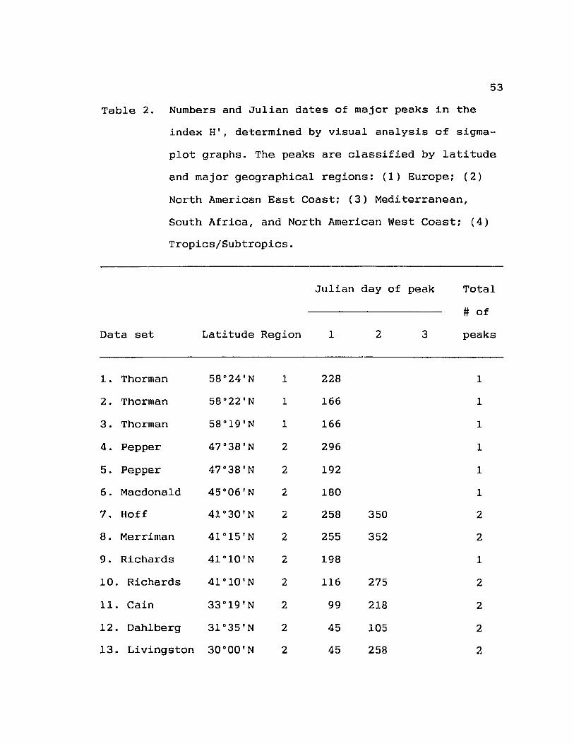
The heterogeneity component of diversity, measured by the

index H' , varied from one to three peaks within an annual

cycle. Two peaks within an annual cycle was the most frequent

pattern; it occurred in six out of the eleven data sets from

the North American region (Table 2 and Figure 7). Figure 7

showed that the interval (in months) between the peaks was

variable and showed no apparent latitudinal trend. However,

the occurrence of the first peaks in H' within an annual cycle

did show a general latitudinal trend; the first peaks occurred

earlier at lower latitudes and later at higher latitudes. That

is, the occurrence of the first peak in H' was in late winter

in the data set from Texas (27°45'N), with the trend generally

progressing over the annual cycle with increasing latitude to

early summer and early fall respectively, in the two data sets

from Newfoundland (47°38'N) (Table 2 and Figure 7).

The occurrence of peaks in the equitability component of

diversity within an annual cycle, as measured by the index E,

is shown in Table 3 and Figure 8. The number of peaks within

53

Table 2. Numbers and Julian dates of major peaks in the

index H', determined by visual analysis of sigma­

plot graphs. The peaks are classified by latitude

and major geographical regions: (1) Europe; (2)

North American East Coast; (3) Mediterranean,

South Africa, and North American West Coast; (4)

Tropics/Subtropics.

Data set Latitude Region

1. Thorman 58°24'N 1

2. Thorman 58°22'N 1

3. Thorman 58°19'N 1

4. Pepper 47°38'N 2

5. Pepper 47°38'N 2

6. Macdonald 45°06'N 2

7. Hoff 41°30'N 2

8. Merriman 41°15'N 2

9. Richards 41°10'N 2

10. Richards 41°10'N 2

11. Cain 33°19'N 2

12. Dahlberg 31°35'N 2

13. Livingston 30°00'N 2

Julian day of peak

1 2 3

228

166

166

296

192

180

258 350

255 352

198

116 275

99 218

45 105

45 258

Total

# of

peaks

1

1

1

1

1

1

2

2

1

2

2

2

2

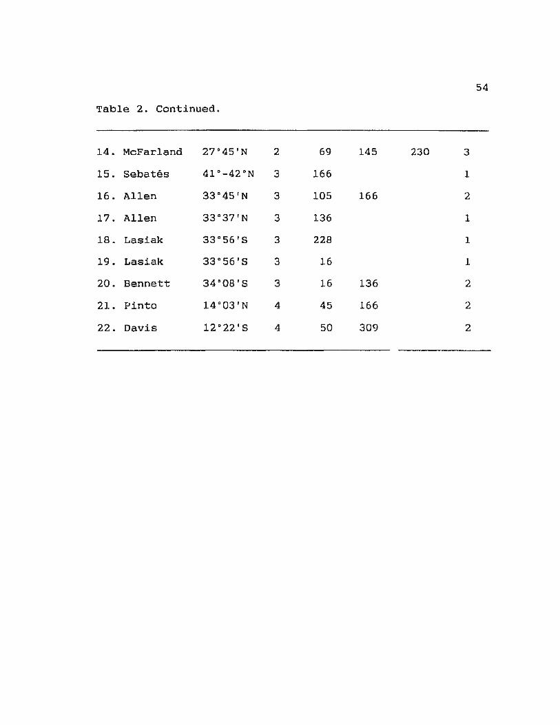
54

Table 2. Continued.

14. McFarland 27•45'N 2 69 145 230 3

15. Sebates 41•-42•N 3 166 1

16. Allen 33"45'N 3 105 166 2

17. Allen 33.37'N 3 136 1

18 . Lasiak 33.56'S 3 228 1

19. Lasiak 33•56'S 3 16 1

20. Bennett 34"08'S 3 16 136 2

21. Pinto 14.03'N 4 45 166 2

22. Davis 12•22'S 4 50 309 2

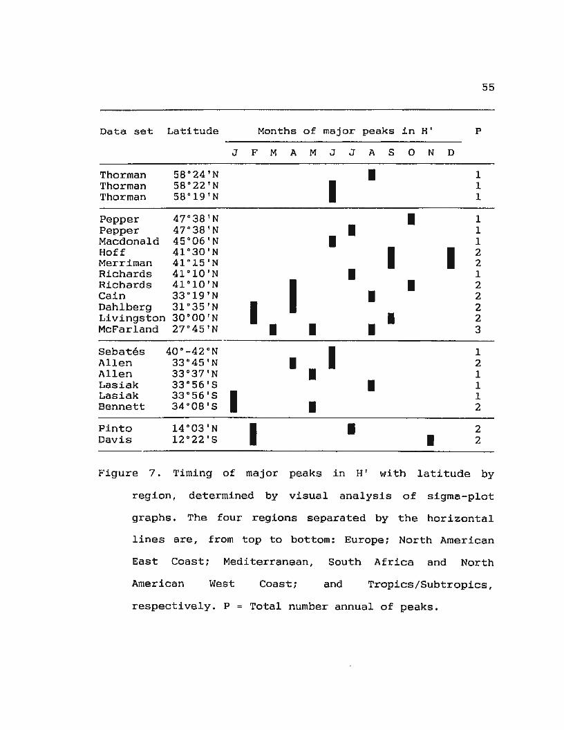
Data set Latitude

Thorman Thorman Thorman

Pepper Pepper Macdonald Hoff Merriman Richards Richards Cain Dahlberg Livingston McFarland

Sebates Allen Allen Lasiak Lasiak Bennett

Pinto Davis

58°24'N 58°22'N 58°19'N

47o38'N 47a38'N 45°06'N 41°30'N 41a15'N 41°10'N 41°10'N 33 a19'N 31°35'N 30°00'N 27o45'N

40°-42°N 33°45'N 33°37'N 33°56'5 33°56'5 34°08'5

Months of major peaks in H'

J F M A M J J A S 0 N D

I I

I I

I I I

I

I I I

I I I I I

I I I

I I I

I I I

p

1 1 1

1 1 1 2 2 1 2 2 2 2 3

1 2 1 1 1 2

2 2

55

Figure 7. Timing of major peaks in H' with latitude by

region, determined by visual analysis of sigma-plot

graphs. The four regions separated by the horizontal

lines are, from top to bottom: Europe; North American

East Coast; Mediterranean, South Africa and North

American West Coast; and Tropics/Subtropics,

respectively. P = Total number annual of peaks.

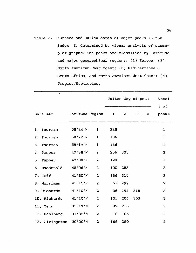
56

Table 3. Numbers and Julian dates of major peaks in the

index E, determined by visual analysis of sigma­

plot graphs. The peaks are classified by latitude

and major geographical regions: (1) Europe; (2)

North American East Coast; (3) MediterrAnean,

South Africa, and North American West Coast; (4)

Tropics/Subtropics.

Data set Latitude Region

1. Thorman 58'24'N 1

2. Thorman 58.22'N 1

3. Thorman 58°19'N 1

4. Pepper 47.38'N 2

5. Pepper 47"38'N 2

6. Macdonald 45.06'N 2

7. Hoff 41°30'N 2

8. Merriman 41"15'N 2

9. Richards 41.10'N 2

10. Richards 41.10'N 2

11. Cain 33°19'N 2

12. Dahlberg 31°35'N 2

13. Livingston 30•00'N 2

Julian day of peak

1 2 3

228

136

166

256 305

129

100 283

166 319

51 299

36 198 318

101 204 303

99 218

16 105

166 350

Total

# of

peaks

1

1

1

2

1

2

2

2

3

3

2

2

2

57

Table 3. Continued.

14. McFarland 27°45'N 2 31 145 188 230 4

15. 8ebates 41°-42"N 3 136 1

16. Allen 33°45'N 3 44 105 2

17. Allen 33°37'N 3 136 1

18. Lasiak 33°56'8 3 197 1

19. Lasiak 33°56'8 3 16 350 2

20. Bennett 34 °08 I 8 3 16 136 2

21. Pinto 14°03'N 4 45 105 166 3

22. Davis 12°22'8 4 62 309 2

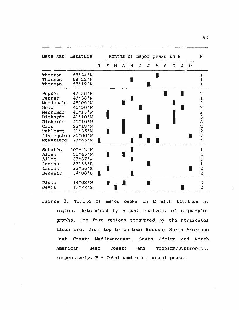
I ' ·~

Data set Latitude Months of major peaks in E

Thorman Thorman Thorman

Pepper Pepper Macdonald Hoff Merriman Richards Richards Cain Dahlberg Livingston McFarland

Sebates Allen Allen Lasiak · Lasiak Bennett

Pinto Davis

J FM AM J J AS 0 N D

58°24'N 58°22'N 58°l9'N

47°38'N 47°38'N 45°06'N 4lo30'N 41°l5'N 4l 0 l0'N 4l 0 l0'N 33°l9'N 31°35'N 30u00'N 27°45'N I

I I

40°-42°N 33°45'N I 33a37'N 33°56'8 33°56's 1 34oo8's 1

I I

I

I I

I I

I I I

I I

I

·-I

I I

I I I

I

I

I I

I I

I

I

I

I

p

1 l l

5B

?. 1 2 2 2 3 3 2 /. 2 4

1 2 1 L 2 7.

3 2

Figure 8. Timing of major peaks in E ~lith la U tude by

region, determined hy visual analysis of sigma-plot:

graphs. The four regions separated by the. horizontal

lines are, from top to bottom: Europe; North Americau

East Coast; Mediterranean, South Africa and North

American West Coast; and Tropics/Suhtropics,

respectively. P = Total number of annual peaks.

59

an annual cycle ranged from one to four. As in H' 1 two peaks

within an annual cycle was the most common pattern. That is,

of the eleven data sets from the North American East Coast

region: two peaks wi th:l.n an annual cycle were observed in

seven data sets; one peak in one data set; three peaks in two

data sets; and four peaks in one data set. Unlike S and H 1 I E

did not show any apparent latitudinal trends in the seasonal

patterns of the occurrence of peaks within an annual cycle

(Figure 8). The sam.a information in each index (date of

occurrence of peaks and number of peaks within an annual

cycle) tested for patterns with habitat type (Tables 4, 5 and

6) and type of gear ( Tabl9s 7 1 8 and 9) showed no apparent

pattern.

3. 4 Spline analysis of seasonal patterns in S, H 1 and E

The timing and number of annual peaks in species richness

s, as measured by spline analysis, showed a general

latitudinal trend in the North American East Coast region. The

occurrence of first peaks was earlier at lower latitudes than

at: higher latitudes. This trend was not progressive with

latitude within each latitudinal division. Generally, the

first peaks occurred earlier (between January and May) at

lower latitudes ( 27 • N to 41"10 'N) while at higher latitudes ( >

<11 o 10 1 N), the peaks occurred later (between June and

September) (Figure 9). Within the higher-latitude division,

Table 4. Numbers and Julian dates of major peaks in the

index S, determined by visual analysis of sigma­

plot graphs. The peaks are classified by habitat

and major geographical regions: (1) Europe; (2)

North American East Coast and Europe; (3)

Mediterranean , South Africa, and North American

West Coast; (4) Tropics/Subtropics.

60

Julian day of peak

Data set Habitat Region 1 2 3

Tota l

# of

peaks

1 . Thorman River 1 258 1

2. Pinto River 4 75 228 25H 3

3. Thorman Estuary 1 289 1

4. Thorman Estuary 1 289 J

5. Hoff Estuary 2 228 1

6. Allen Estuary 3 197 J

7. Cain Estuary 2 99 247 2

8. Dahlberg Estuary 2 136 289 2

9. Davis Estuary 4 50 280 3 5 5 3

10. Pepper Inshore 2 296 L

11. Pepper Inshore 2 192 ]

12 . Macdonald Inshore 2 165 ]

13. Merriman Inshore 2 225 304 352 3

61

Table 4. Continued.

14. Richards Inshore 2 147 289 2

15. Richards Inshore 2 147 289 2

16. Allen Inshore 3 166 1

17. McFarland Surf-zone 2 145 283 2

18. Lasiak Surf-zone 3 105 319 2

19. Lasialt Surf-zone 3 105 289 350 3

20. Bennett Surf-zone 3 350 1

21. Livingston Salt marsh 2 45 258 2

22. Sebates Shelf /Pelagic 3 166 1

62

Table 5. Numbers and Julian dates of major peaks in the

indeK H', determined by visual analysis of sigma­

plot graphs. The peaks are classified by habitat

and major geographical regions: (1) Europe: (2)

North American East Coast: (3) Mediterranean,

South Africa, and North American West Coast; (4)

Tropics/Subtropics.

Data set

1. Thorman

2. Pinto

3. Thorman

4. Thorman

5. Hoff

6. Allen

7. Cain

8. Dahlberg

9. Davis

10. Pepper

11. Pepper

12. Macdonald

13. Merriman

Julian day of peak

Habitat Region 1 2 3

River 1 228

River 4 45 166

Estuary 1 166

Estuary 1 166

Estuary 2 258 350

Estuary 3 136

Estuary 2 99 218

Estuary 2 45 105

Estuary 4 50 309

Inshore 2 296

Inshore 2 192

Inshore 2 180

Inshore 2 225 352

'l'otal

# of

peaks

1

2

1

1

2

1

2

2

2

1

1

1

2

63

Table 5. Continued.

14. Richards Inshore 2 198 1

15. Richards Inshore 2 166 275 2

16. Allen Inshore 3 105 166 2

17. McFarland Surf-zone 2 69 145 230 3

18. Lasiak Surf-zone 3 228 1

19. Lasiak Surf-zone 3 16 1

20. Bennett Surf-zone 3 16 136 2

21. Livingston Salt marsh 2 45 258 2

22. Sebates Shelf/Pelagic 3 166 1

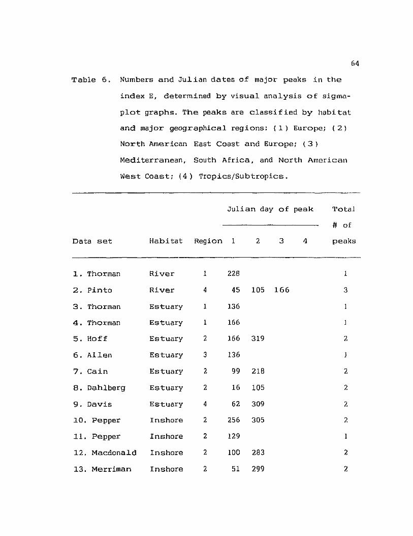
Table 6. Numbers and Julian dates o£ major peaks in the

index E, determined by visual analysis of sigma­

plot graphs. The peaks are classified by habitat

and major geographical regions: ( 1) Europe; ( 2)

North American East Coast and Europe; ( 3 )

Mediterranean, South Africa, and North American

~Jest Coast; ( 4) Tropics/Subtropics.

64

Julian day of peak •rota1

Data set Habitat Region 1

1. Thorman River 1 228

2. Pinto River 4 45

3. Thorman Estuary 1 136

4. Thorman Estuary 1 166

5. Hoff Estuary 2 166

6. Allen Estuary 3 136

7. Cain Estuary 2 99

8. Dahlberg Estuary 2 16

9. Davis Estuary 4 62

lO. Pepper Inshore 2 256

ll. Pepper Inshore 2 129

12. Macdonald Inshore 2 100

13. Merriman Inshore 2 51

2 3

105 166

319

218

105

309

305

283

299

4

# of

penks

1

3

2

J

2

2

2

2

2

2

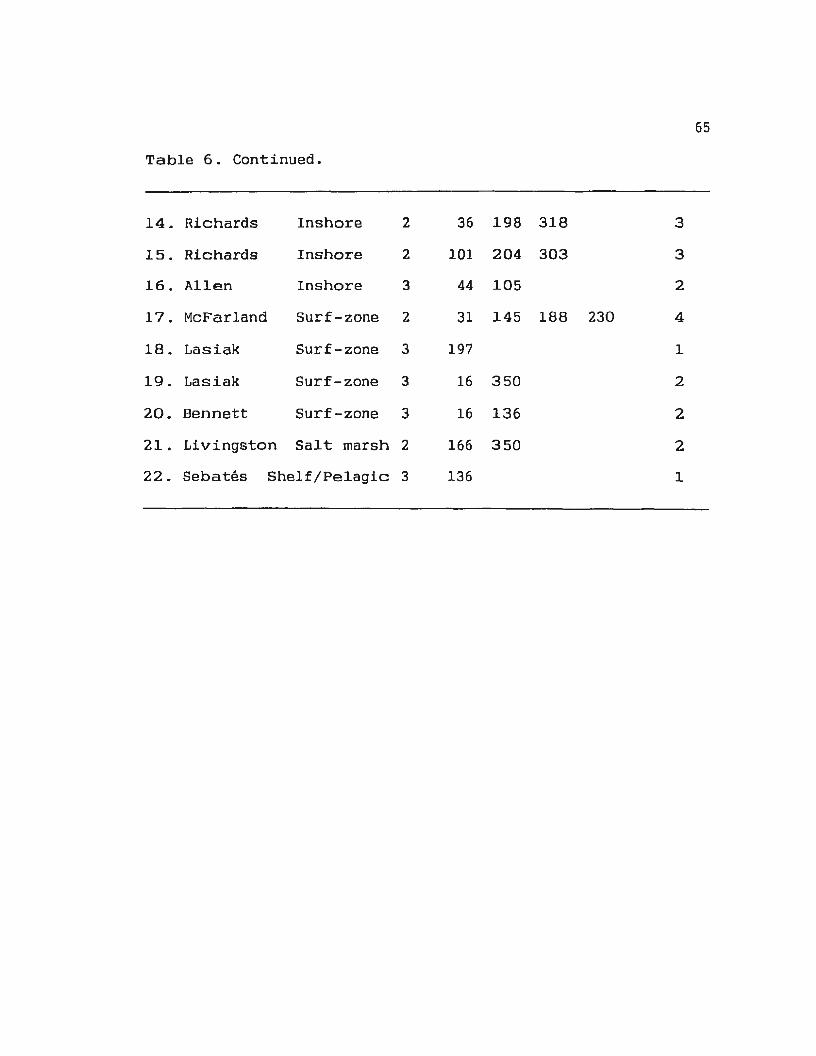
65

Table 6. Continued.

14. Richards Inshore 2 36 198 318 3

15. Richards Inshore 2 101 204 303 3

16. Allen Inshore 3 44 105 2

17. McFarland Surf-zone 2 31 145 188 230 4

18. Lasiak Surf-zone 3 197 1

19 . Lasiak Surf-zone 3 16 350 2

20. Bennett Surf-zone 3 16 136 2

21. Livingston Salt marsh 2 166 350 2

22. Sebates Shelf/Pelagic 3 136 1

66

Table 7. Numbers and Julian dates of major peaks in the

index S, determined by visual analysis of sigma­

plot graphs. The peaks are classified by gear type

and major geographical regions: ( 1 ) Europe; ( 2)

North American East Coast; ( 3) Mediterranean,

South Africa, and North American West Coast; {11)

Tropics/Subtropics.

Julian day of peak 'l'ot a l

Date. set Gear Region 1 2 3

# of

peaks

1. Merriman Trawl 2 225 304 352 3

1. Richards Trawl 2 147 289 2

3. Richards Trawl 2 147 289 2

4. Dahlberg Trawl 2 136 289 2

5. Pinto Trawl 4 75 228 25fl 3

6. Macdonald Seine 2 165 1

7. Hoff Se ine 2 228 1

B. Allen Seine 3 166 l

9. Allen 'Mixture'* 3 197 1

10. McFarland Seine 2 145 238 2

11. Lasiak Seine 3 105 319 ?.

12. Lasi ak Seine 3 105 289 350 3

13. Bennett Seine 3 3 50 1

Table 7. Continued.

14.

15.

16.

17.

18.

19.

20.

21.

22.

*

Thorman Drop net 1 258 1

Thorman Drop net 1 289 1

Thorman Drop net 1 289 1

Davis Flood trap 4 50 280 355 3

Sebates Bongo net 3 166 1

Pepper Scuba census 2 296 1

Pepper Scuba census 2 192 1

Cain Poison 2 99 247 2

Livingston r.oison 2 45 258 2

A mixture of sampling gears wi th known effort were used. The gears included a Bag seine, Seine, Drop net and Enclosure net.

67

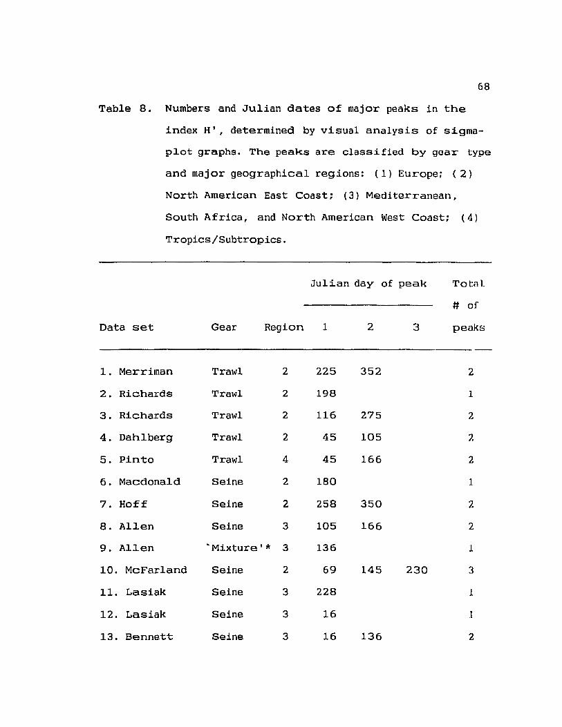
68

Table 8. Numbers and Julian dates of major peaks in the

index H 1 1 determined by visual analysis of sigma­

plot graphs. The peaks are classified by gear type

and major geographical regions: ( 1) Europe: ( 2)

North American East Coast; ( 3) Mediterranean I

South Africa 1 and North American West Coast; ( 4)

Tropics I Subtropics.

Data set Gear Region

1. Merriman Trawl 2

2. Richards Trawl 2

3. Richards Trawl 2

4. Dahlberg Trawl 2

5. Pinto Trawl 4

6. Macdonald Seine 2

7. Hoff Seine 2

8. Allen Seine 3

9. Allen 'Mixture 1 * 3

10. McFarland Seine 2

11. Lasiak Seine 3

12. Lasiak Seine 3

13. Bennett Seine 3

Julian day of peak

1 2 3

225 352

198

116 275

45 105

45 166

180

258 350

105 166

136

69 145 230

228

16

16 136

To tn 1.

# of

peaks

2

1

2

2

2

1

2

2

1

3

1

1

2

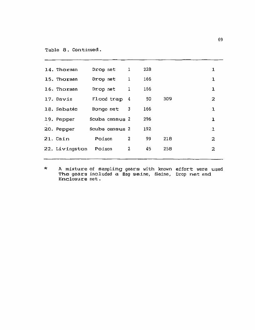
69

Table 8. Continued.

14. Thorman Drop net 1 228 1

15. Thorman Drop net 1 166 1

16. Thorman Drop net 1 166 1

17. Davis Flood trap 4 50 309 2

18. Sebateo Bongo net 3 166 1

19. Pepper Scuba census 2 296 1

20. Pepper Scuba census 2 192 1

21. Cain Poison 2 99 218 2

22. Livingston Poison 2 45 258 2

* A mixture of sampling gears with known effort were used The gears included a Bag seine, Seine, Drop net and Enclosure net •

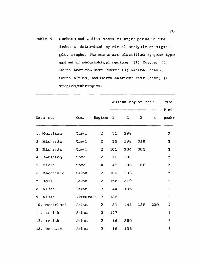
70

Table 9. Numbers and Julian dates of major peaks in the

indeK E, determined by visual analysis of sigma­

plot graphs. The peaks are classified by gear type

and major geographical regions: ( 1) Europe; ( 2)

North American East Coast; ( 3 ) Medi terranean,

South Africa, and North American West Coast; ( 4)

Tropics/Subtropics.

Data set

1. Merriman

2. Richards

3. Richards

4. Dahlberg

5. Pinto

6. Macdona ld

7. Hoff

8. Allen

9. Allen

10. McFarland

11. Lasiak

12. Lasiak

13. Bennet t

Julian day of peak

Gear Region 1 2 3 4

Trawl 2 51 299

Trawl 2 36 198 31 8

Trawl 2 101 204 303

Trawl 2 16 105

Trawl 4 45 105 166

Seine 2 100 283

Seine 2 166 319

Seine 3 44 105

'Mixture'* 3 136

Seine 2 31 145 188 230

Sei.ne 3 197

Sei ne 3 1 6 350

Seine 3 16 136

'fatal

# of

peaks

?.

3

3

2

3

2

2

2

J.

11

1

2

2

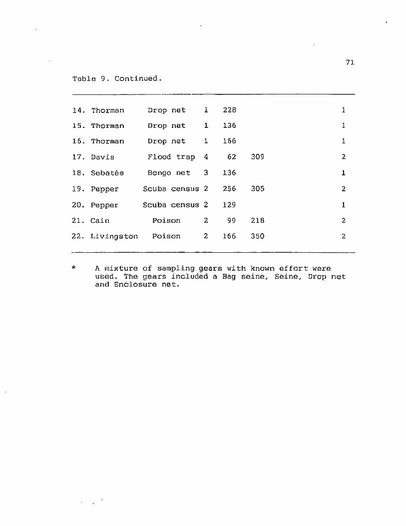
Table 9. Continued.

14. Thorman Drop net l 228 1

15. Thorman Drop net 1 136 1

16. Thorman Drop net 1 166 1

17. Davis Flood trap 4 62 309 2

18. Sebates Bongo net 3 136 1

19. Pepper Scuba census 2 256 305 2

20. Pepper Scuba census 2 129 1

21. Cain Poison 2 99 218 2

22. Livingston Poison 2 166 350 2

* A mixture of sampling gears with known effort were used. The gears included a Bag seine, Seine , Drop net and Enclosure net.

71

Data set Latitude Months of major peaks in S

J F M A M J J A S 0 N D

Thorman Thorman Thorman

58°24'N 58°22'N 58°19'N

I

I I

I I

I I •

Pepper Pepper Macdonald Hoff Merriman Richards Richards Cain Dahlberg Livingston McFarland

47°38'N 47o38'N 45°06'N 41°30'N 41°15'N 4l 0 10'N 41ol0'N 33°19'N 31°35'N 30°00'N 27°45'N

I I I

I I

I I

I I I

Sebates Allen Allen Lasiak Lasiak Bennett

Pinto Davis

40o-42oN 33°45'N 33a37'N 33°56'S 33°56'S 34°08'S I

I

I I I

I

+ Splines fitted with a 15 days resolution; ++ Splines fitted with a 30 days resolution;

I

I

All others were fitted with a 60 days resolution.

p

l 0 I

72

7. ·I 2 I 1 ~I I

3+1 2 2 3 2·1 ·I

I I I I. 1 I

I. 1·H

Figure 9. Timing of major peaks in S with latitude by

region, determined by spline analysis. 'rhe four regions

separated by the horizontal lines are, from top to

bottom: Europe; North American East Coast; Mediterranean,

South Africa and North American West Coast; and

Tropics/Subtropics. P ; Number of annual peaks.

73

the first peaks occurred earlier at higher latitudes and later

at lower latitudes (Figure 9). This contrasts with the general

pattern of earlier peaks at lower latitudes and later peaks at

higher latitudes, observed between the two latitudinal

divisions. The position of this change in the timing of the

occurrence of the first peak inS between the two latitudinal

divisions seem to be at about 41°10' N (Figure 9). In addition

to differences in the timing of the first annual peaks in the

index S, there were generally two or more peaks in the index

within an annual cycle at latitudes less than and equal to

41°10'N, while at latitudes greater than 41.10'N there were

between one and two peaks within an annual 0ycle.

The timing of the first peak in heterogeneity H', also

appeared to occur earlier at lower latitudes (27•N to 41.15'N)

than at higher latitudes (> 41.15'N) in the North American

East Coast region (Figure 10). In comparison to the latitude

of separation between higher and lower latitudes in S, which

is 41.10'N, the latitude of 41"15'N for H' is comparable in

this respect. The occurrence of the first peaks ranged between

January and April at lower latitudes (27.45'N to 41.15'N) in

this region while at the higher latitudes ( > 41 • 15 'N) i "\.:

ranged between July and October (Figure 10). As in the species

richness index S, there was a tenden.-:y for the data sets from

higher latitudes(> 41"15'N) in the North American East Coast

region to have up to two peaks \'li thin an annual cycle while two

Data set Latitude Months of major peaks in H'

J F M A M J J A S 0 N D

Thorman Thorman Thorman

Pepper Pepper Macdonald Hoff Merriman Richards Richards Cain Dahlberg Livingston McFarland

Sebates Allen Allen Lasiak Lasiak Bennett

Pinto Davis

58°24'N 58°22'N 58°19'N

47°38'N 47°38'N 45°06'N 41°30'N 41°15'N 4lol0'N 41°10'N 33a19'N 31°35'N 30°00'N 27°45'N

40°-42oN 33°45'N 33°37'N 33°56'8 33°56'8 34°08'8

I

I

I

I

I

I

I I

I I

I I

I

I

I I

I

I

I

I

I

I

I

I I

I

+ Splines fitted with a 15 days resolutinn; ++ Splines fitted with a 30 days resolution;

I I

I

I

I

I

I

I

All others were fitted with a 60 days resolution.

p

1 1 l

74

2 t·

2 J 2 2+ I

4 I I

2 1 /. 5t·l

J 2 2 t1 J 1

2 lH

Figure 10. Timing of major peaks ir. H' with latitude by

region, determined by spline analysis. The four regions

separated by the horizontal lines are, from top to

bottom: Europe; North Ame1.:-ican East Coast; Mediterranean,

South Africa and North American West Coast; and

Tropics/Subtropics. P = Number of annual peaks.

75

or more peaks appeared to occur at lower latitudes (s

4ln15'N).

The equitability component of diversity measured by the

index E also showed a trend similar to Sand H', regarding the

timing of the occurrence of the first peak (Figure 11). At

lower latitudes (S 4l 0 15'N) the months of first peaks ranged

between January and April. Similar peaks at higher latitudes

(> 4l 0 l5'N) ranged between March and April (Figure 11). Three

annual peaks in the equitability index E was more common in

the North American East Coast region.

The latitudinal trend in the time of occurrence of the

first peak in all three indices was more obvious than that for

the number of major peaks in the three indices, in the North

American East Coast region. That is, the first annual peaks in

S, H' and E generally occurred earlier at lower latitudes (s

41.10'N) than at higher latitudes(> 41°l0'N) within an annual

cycle (Tables 10, 11 and 12; Figures 9, 10 and 11). This trend

in the time of occurrence of the peaks with latitude was more

apparent in the heterogeneity H' and equitability E components

of diversity but less so in the species richness S component

of di•!ersity. This is evident form the regressions of Julian

dates of first peaks in each index with latitude (Figures 12,

13 and 14). The coefficients of determination (r2 ), which are

measures of explained variances in the regressions, were 0.11

(p = 0.351), 0.28 (p = 0.114), and 0.25 (p = 0.145) for S, H'

Data set Latitude Months of major peaks in E

J F M A M J J A S 0 N D

Thorman Thorman Thorman

Pepper Pepper Macdonald Hoff Merriman Richards Richards Cain Dahlb•arg Livingston McFarland

Sebates Allen Allen Lasiak Lasiak Bennett

Pinto Davis

58°24'N 58.22'N 58°19'N

47°38'N 47°38'N 45°06'N 41°30'N 4l 0 l5'N 41°10'N 4l 0 10'N 33°19'N 3lo35'N 30°00'N 27°45'N

40°-42°N 33°45'N 33°37'N 33°56'8 33°56'S 34°08'S

I

I

I I

I

I

I

I

I

I

I

I I

I

I

I I I

I I I

I I I

I I

I I

+ Splines fitted with a 15 days resolution; ++ Splines fitted with a 30 days resolution;

I

I

I

I I

I

I

I

All others were fitted with a 60 days resolution.

p

1 .l 1

76

3-f 2 2 3 Jl-t I

3t- .. 2 1 3 3 + t

1 2 2 11 2 L

2 1 ·I I

Figure 11. Timing of major peaks in E with l atitude by

region, determined by spline analysis. The four regions

separated by the horizontal lines are, from top to

bottom: Europe; North American East Coast; Medi terrancan,

South Africa and North American West Coa s t; a nd

Tropics/Subtropics. P = Number of annual peaks.

77

Table 10. Number and Julian dates of major peaks in the

index S, determined by spline analysis. The peaks

are classified by latitude and major geographical

regions: (1) Europe; (2) North American East

Coast; (3) Mediterranean, South Africa, and North

American West Coast; (4) Tropics/Subtropi cs.

Data set Latitude Region

1. Thorman 58°24'N 1

2. Thorman 58°22'N 1

3. Thorman 58 °19'N 1

4. Pepper 47 °38'N 2

5. Pepper 47°38'N 2

6. Macdonald 45°06'N 2

7. Hoff 41 °30'N 2

8. Mer riman 41 °15'N 2

9. Richards 41°10'N 2

10. Richa rds 41°10'N 2

11. Cain 33°19'N 2

12. Dahlberg 31 °35'N 2

13. Livingston 30 °00'N 2

14. McFarland 27 a45'N 2

Julian day of peak

1 2 3 4 5

166

0

166

206 297

194 283

228

255

81 147 226 289 338

18 83 226

99 290

197 289

45 105 258

145 2 58

Total

# of

peaks

1

0

1

2+

2

1

1

5++

3+ +

2

2

3

2++

Table 10. Continued.

15. Sebates 40°-42oN 3 166

16. Allen 33"45'N 3 136

17. Allen 33"37'N 3 136

18. Lasiak 33"56'S 3 105 319

19. Lasiak 33"56'S 3 105

20. Bennett 34"08'S 3 16

21. Pinto 14"03'N 4 16 258

22. Davis 12°22'S 4 355

+ Splines fitted with a resolution of 15 days; ++ Splines fitted with a resolution of 30 days:

All others were fitted with a resolution of 60 days.

78

1

1

1

2

1

2

I + t

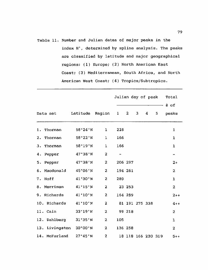
79

Table 11. Number and Julian dates of major peaks in the

index H', determined by spline analysis. The peaks

are classified by latitude and major geographical

regions: (1) Europe; (2) North American East

Coast; (3) Mediterranean, South Africa, and North

American West Coast; (4) Tropics/Subtropics.

Julian day of peak Total

# of

Data set Latitude Region 1 2 3 4 5 peaks

1. Thorman 58°24'N 1 228 1

2. Thorman 58°22'N 1 166 1

3. Thorman 58°19'N 1 166 1

4. Pepper 47°38'N 2

5. Pepper 47°38'N 2 206 297 2+

6. Macdonald 45°06'N 2 194 261 2

.... Hoff 41°30'N 2 289 1 I •

8. Merriman 41°15'N 2 23 253 2

9. Richards 41°10'N 2 164 289 2++

10. Richards 41°10'N 2 81 191 275 338 4++

11. Cain 33°19'N 2 99 218 2

12. Dahlberg 31°35'N 2 105 1

13. Livingston 30°00'N 2 136 258 2

14. McFarland 27°45 1 N 2 18 118 166 230 319 5++

Table 11. Continued.

15. Sebates 40°-42°N 3 166

16. Allen 33°45'N 3 105 289

17. Allen 33°37'N 3 136 289

18. Lasiak 33°56'S 3 16 105 228 319

19. Lasiak 33°56'8 3 45

20. Bennett 34°08'8 3 16

21. Pinto l4°03'N 4 75 289

22. Davis 12°22'8 4 ~)0

+ Splines fitted with a resolution of 15 days; ++ Splines fitted with a resolution of 30 days;

80

1

2

2

t1

1.

1

2

1++

All others were fitted with a resolution of 60 days.

81

Table 12. Number and Julian dates of major peaks in the

index E, determined by spline analysis. The peaks

are classified by latitude and major geographical

regions: (1) Europe; (2) North American East

Coast; (3) Mediterranean, South Africa, and North

American West Coast; (4) Tropics/Subtropics.

Data set Latitude Region

1. Thorman 58"24'N 1

2. Thorman 58"22'N 1

3. Thorman 58"19'N 1

4. Pepper 47"38'N 2

5. Pepper 47"38'N 2

6. Macdonald 45°06'N 2

7. Hoff 41°30 IN 2

8. Merriman 41°15'N 2

9. Richards 4l 0 10'N 2

10. Richards 41°10'N 2

11. Cain 33°19'N 2

12. Dahlberg 31"35'N 2

13. Livingston 30"00'N 2

14. McFarland 27"45'N 2

Julian day of peak

1 2 3 4

228

166

166

129 241 341

100 283

105 319

23 83 253

36 116 191 318

81 226 303

99 218

105

16 136 197

13 118 230

Total

# of

peaks

1

1

1

3+

2

2

3

4++

3++

2

1

3

3++

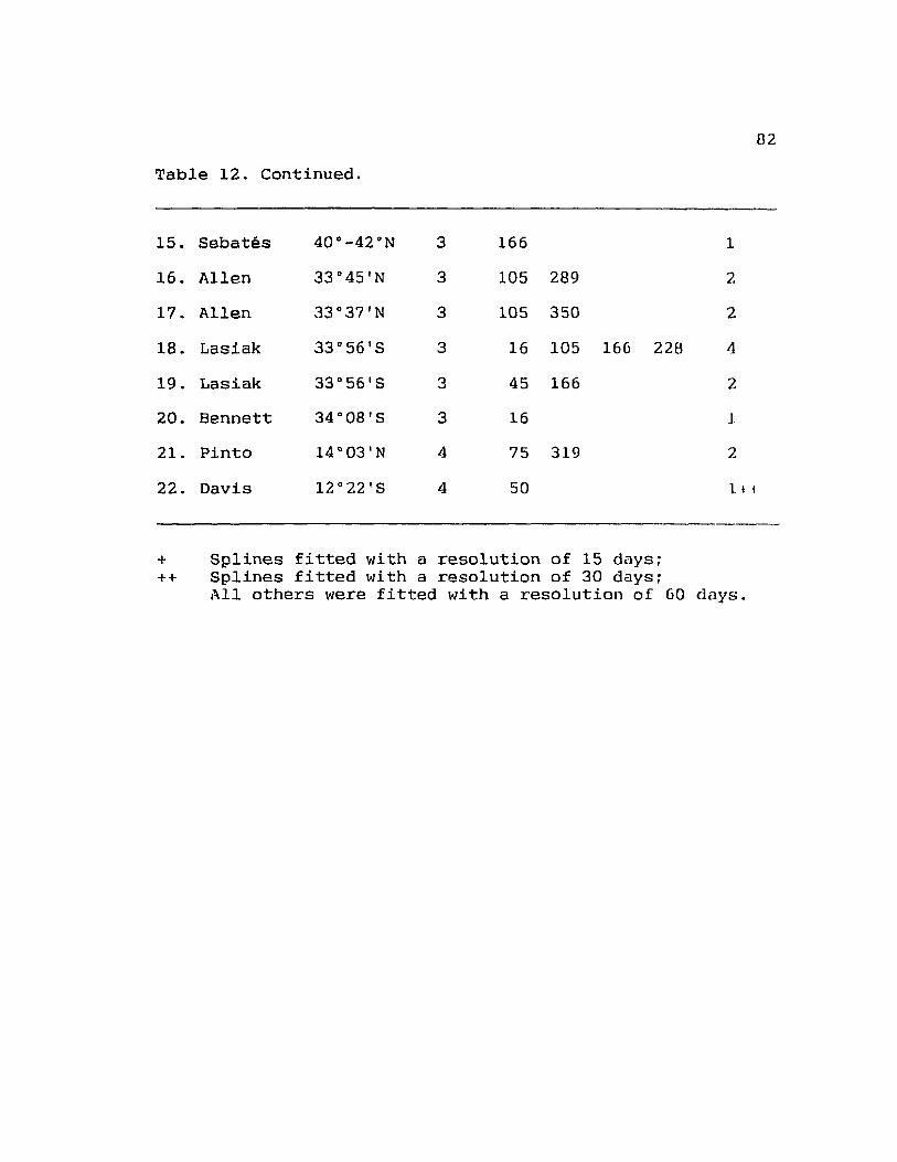
Table 12. Continued.

15. 8ebates 40°-42°N 3 166

16. Allen 33°45'N 3 105 289

17. Allen 33°37'N 3 105 350

18. Lasiak 33°56'8 3 16 105 166 228

19. Lasiak 33°56'8 3 45 166

20. Bennett 34°08'8 3 16

21. Pinto 14°03'N 4 75 319

22. Davis 12°22'8 4 50

+ Splines fitted with a resolution of 15 days; ++ Splines fitted with a resolution of 30 days;

1

2

2

4

2

1

2

ll I

All others were fitted with a resolution of 60 days.

02

Figure 12. Regression of Julian day of first peak in

s with latitude. The coefficient of

determination (r2 ) of the regression is

0.11 (p=0.351).

300

250 • •

(/) 200 • ~

• • 0 z 150 <( :J :::> "") 100 •

•

50 • •

0 25 30 35 40 45 50

LATITUDE (DEGREES NORTH)

Figure 13. Regression of Julian day of first peak in H'

with latitude. The coefficient of

determination (r2 ) of the regression is 0 . 28

(p=0.114).

300 •

250

200 • (/)

~ 0 150 z <1: :J ~ 100 """)

50

• • 0

25 30 35 40 45 50

LATITUDE (DEGREES NORTH)

Figure 14. Regression of Julian day of first peak in E

with latitude. The coefficient of

determination (r2 ) of the regression is 0.25

( p=O. 145).

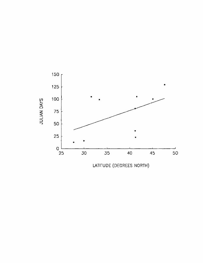
150

125 •

• • Vl 100 • ~ ~

---~ 0

z 75 <t _J

:::> J 50

• 25 •

• • 0 25 30 35 40 45 50

LATITUDE (DEGREES NORTH)

89

and E, respectively. Taking into account the fact that the

data used for the regressions were from an inevitably limited

number of field, not experimental, studies an a :5 0.15 is

accepted as significant. A significance criterion of a s 0.15

was used in this exploratory analysis, in order to reduce Type

II error, failure to detect a true pattern. Even if taking a

:5 0.05, a conservative level traditionally accepted in

hypothesis testjng, renders these regressions non-significant,

Figures 12, 13 and 14 do indicate a latitudinal trend in the

northward progression of the dates of first peaks in s, II ' and

E.

The slope of the regressions for H' and E were 6.58 and

3.19 days per degree north, respectively. These slopes can be

interpreted as the rate of northward progression of the

occurrence of first peaks in heterogeneity and equitability in

an annual cycle. As evident from the coefficients of

determination, only dates of occurrence of first peaks in

heterogeneity H' and equi tabili ty E showed a trend with

latitude but not species richness S. The number of peaks was

variable between lower and higher latitudes. On the whole, two

annual peaks in species richness s, he terogene.i ty II' a nd

equi tabili ty E commonly occurred at higher latitudes in the

North American East Coast region. Two to three peaks r,.mre

generally noted in the three indices at lower latitudes Jn

this regard.

90

The position of the latitudinal division for "northern'

and ·southern' latitudes was lower ( 41 a 10' N) for S, while

forH' and E it was at 41°15'N. This difference by only 5' is

a minor one. However, this latitudinal position does coincide

with the approximate latitudinal range (4loN- 42°N) at which

the cooler (soc - l0°C) "bore-al" water masses separate from

the warmer ( 10oc - 25°C) "warm temperate" waters (Hedgpeth,

1957; Colton, 1964 QQ Qit. Colton et al., 1979; Backus, 1986);

·the temperature ranges given for the two water masses are

taken from Figure 5 of Hedgpeth ( 1957). The trend for the

number of peaks to be more than two within an annual cycle at

lower latitudes was stronger for S and H' than E.

Tables 10, 11, and 12 summarize the timing and number of

annual peaks in S, H' and E respect! vely, which were

determined by spline analysis. The timing and number of annual

peaks are compared with respect to latitude. Similar summaries

for S, H' and E are given for the testing for relationships

with habitat (Tables 13, 14, and 15) and type of gear (Tables

16, 17, and 18). The information in Tables 10, 11, and 12

agreed with the patterns described above using Figures 9, 10,

and 11. There was no apparent ~e1ationship in the timing of

seasonal peaks in S, H' and E with habitat type (Tables 13,

14, and 15) or type of gear used (Tables 16, 17, and 18).

However, there was a relationship in the two variables with

the total number of peaks in an annual cycle for all

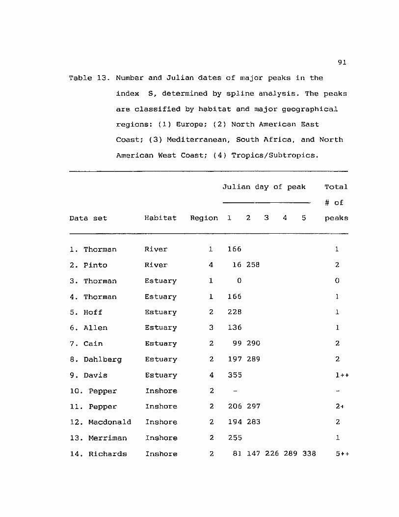
91

Table 13. Number and Julian dates of major peaks in the

index S, determined by spline analysis. The peaks

are classified by habitat and major geographical

regions: (1) Europe; (2) North American East

Coast; (3) Mediterranean, South Africa, and North

American West Coast; (4) Tropics/Subtropics.

Data set Habitat

1. Thorman River

2. Pinto River

3. Thorman Estuary

4. Thorman Estuary

5. Hoff Estuary

6. Allen Estuary

7. Cain Estuary

8. Dahlberg Estuary

9. Davis Estuary

10. Pepper Inshore

11. Pepper Inshore

12. Macdonald Inshore

13. Merriman Inshore

14. Richards Inshore

Julian day of peak

Region 1 2 3 4 5

1 166

4 16 258

1 0

1 166

2 228

3 136

2 99 290

2 197 289

4 355

2

2 206 297

2 194 283

2 255

2 81 147 226 289 338

Total

# of

peaks

1

2

0

1

1

1

2

2

1++

2+

2

1

5 ++

Table 13. Continued.

15. Richards Inshore 2 18 83 226

16. Allen Inshore 3 136

17. McFarland Surf-zone 2 145 258

18. Lasiak Surf-zone 3 105 319

19. Lasiak Surf-zone 3 105

20. Bennett Surf-zone 3 16

21. Livingston Salt marsh 2 45 105 258

22. Sebates Shelf/Pelagic 3 166

+ Splines fitted with a resolution of 15 days; ++ Splines fitted with a resolution of 30 days;

All others were fitted with a resolution of 60 days.

92

3++

1

2++

2

1

1

3

1

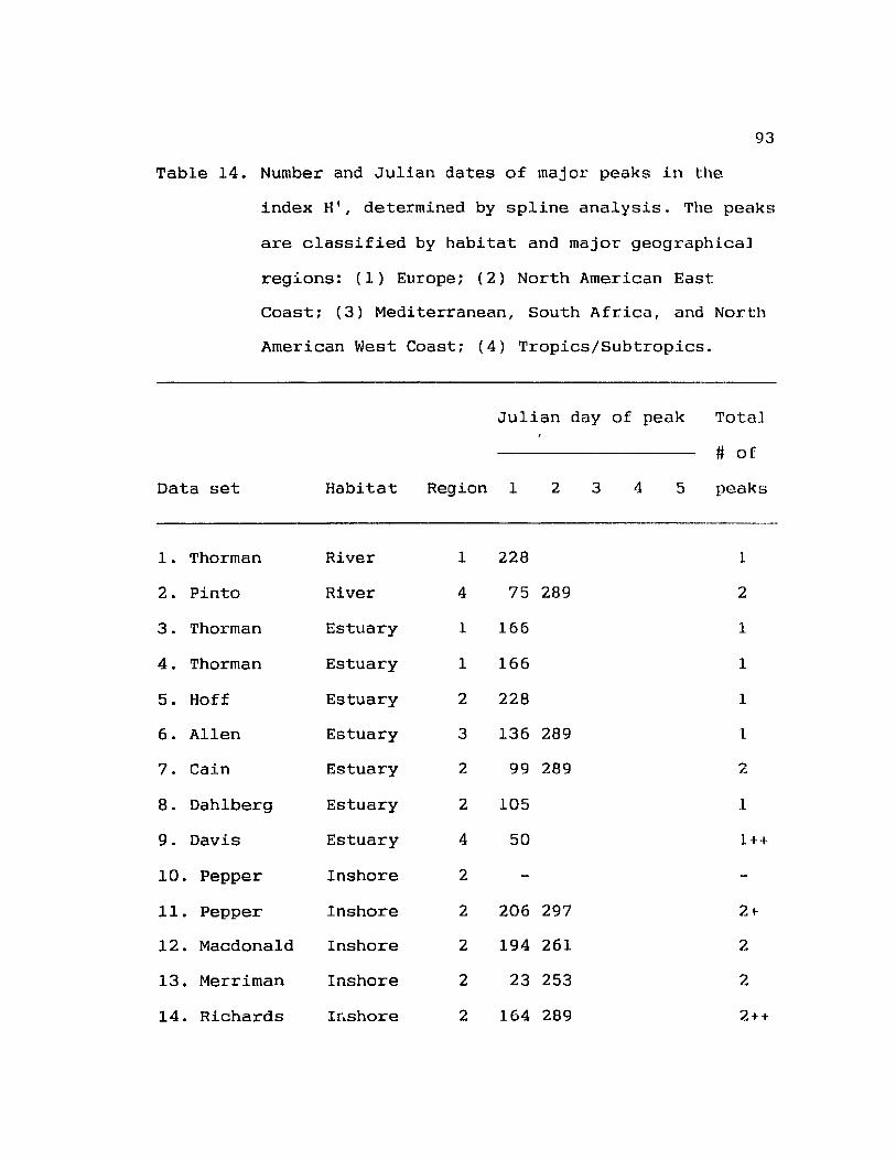
93

Table 14. Number and Julian dates of major peaks in the

index H' , determined by spline analysis. The peaks

are classified by habitat and major geographical

regions: (1) Europe; (2) North American East

Coast; (3) Mediterranean, South Africa, and North

American West Coast; (4) Tropics/Subtropics.

Julian day of peak Tot a]

# o f

Data set Habitat Region 1 2 3 4 5 peaks

1. Thorman River 1 228 1

2. Pinto River 4 75 289 2

3. Thorman Estuary 1 166 1

4. Thorman Estuary 1 166 1

5. Hoff Estuary 2 228 1

6. Allen Estuary 3 136 289 l

7. Cain Estuary 2 99 289 " L.

8. Dahlberg Estuary 2 105 1

9. Davis Estuary 4 50 1 ++

10. Pepper Inshore 2

11. Pepper Inshore 2 206 297 2+-

12. Macdonald Inshore 2 194 261 2

13. Merriman Inshore 2 23 253 2

14. Richards I r.shore 2 164 289 2++

Table 14. Continued.

15. Richards Inshore 2 81 191 275 338

16. Allen Inshore 3 105 289

17. McFarland Surf-zone 2 18 118 166 230

18. Lasiak Surf-zone 3 16 105 228 319

19. Lasiak Surf -zone 3 45

20. Bennett Surf-zone 3 16

21. Livingston Salt marsh 2 136 258

22. Sebates Shelf/Pelagic 3 166

+ Splines fitted with a resolution of 15 days ; ++ Spl ines f i tted with a resol u t ion of 30 days ;

94

4 ++

2

319 5++

2

1

1

2

1

All others were fitted with a resolution o f 60 days.

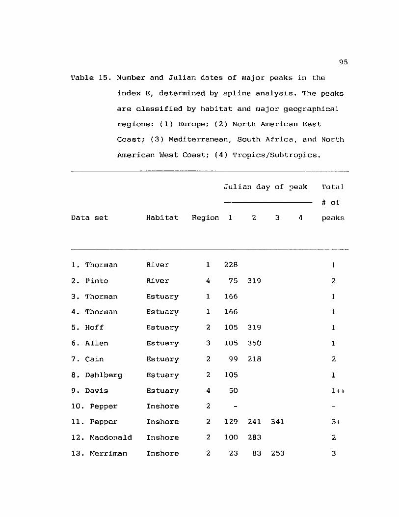
95

Table 15. Number and Julian dates of major peaks in the

index E, determined by spline analysis. The peaks

are classified by habitat and major geographical

regions: (1) Europe; (2) North American East

Coast; (3} Mediterranean , South Africa, a nd No r. lh

American West Coast; (4} Tropics/Subtropics.

Data set Habitat

1. Thorman River

2. Pinto River

3. Thorman Estuary

4. Thorman Estuary

5. Hoff Estuary

6 . Allen Estuary

7. Cain Estuary

8. Dahlberg Estuary

9. Davis Estuary

10. Pepper Inshore

11. Pepper Inshore

12. Macdonald Inshore

13. Merriman Inshore

Julian day of ~eak

Region 1 2 3

1 228

4 75 319

1 166

1 166

2 105 319

3 105 350

2 99 218

2 105

4 50

2

2 129 241 341

2 100 283

2 2 3 83 253

Totul

# o f

pea k s

:7.

I

1

1

1

2

1

1 ++

3-+

2

3

Table 15. Continued.

14. Richards Inshore 2 36 116 191 318

15. Richards Inshore 2 81 226 303

16. Alle-.n Inshore 3 105 289

17. McFarland Surf-zone 2 13 118 230

18. Lasiak Surf-zone 3 16 105 166 228

19. Lasiak Surf-zone 3 45 166

20. Bennett Surf-zone 3 16

21. Livingston Salt marsh 2 16 136 197

22. SeLates Shelf/Pelagic 3 166

+ Splines fitted with a resolution of 15 days; ++ Spllnes fitted with a resolution of 30 days;

96

4++

3++

2

3++

4

2

1

3

1

All others were fitted with a resolution of 60 days.

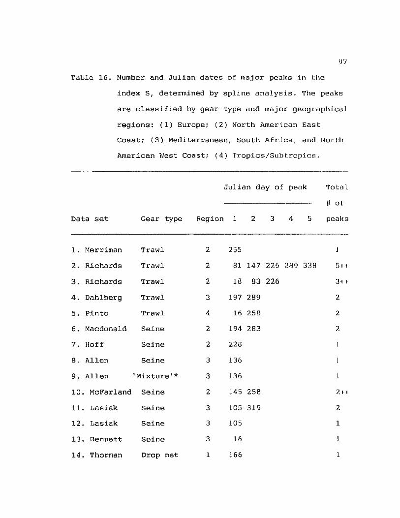
1)7

Table 16. Number and Julian daten of major peaks in the

index S, determined by spline analysis. The peaks

are classified by gear type and major geographical

regions: (1) Europe: (2) North Ameri..can East

Coast; (3) Mediterranean, South Africa, and North

American West Coast; (4) Tropics/Subtropics.

Data set Gear type

1. Merriman Trawl

2. Richards Trawl

3. Richards Trawl

4. Dahlberg Trawl

5. Pinto Trawl

6. Macdonald Seine

7. Hoff Seine

8. Allen Seine

9. Allen 'Mixture'*

10. McFarland Seine

11. Lasiak Seine

12. Lasiak Seine

13. Bennett Seine

14. Thorman Drop net

Julian day of peak

Region 1 2 3 4 5

2 255

2 81 147 225 289 338

2 1t3 83 226

:2 197 289

4 16 258

2 194 283

2 228

3 136

3 136

2 145 258

3 105 319

3 105

3 16

1 166

Total

# of

peaks

1

51-1

3-i ..

2

2

7.

1

?, I I

2

1

1

1

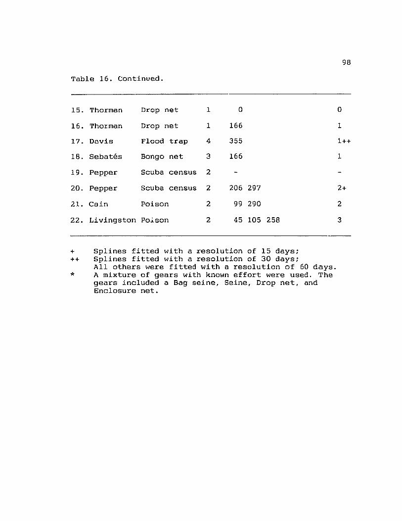
Table 16. Continued.

15. Thorman Drop net 1 0

16. Thorman Drop net 1 166

17. Dnvis Flood trap 4 355

18. Sebates Bongo net 3 166

19. Pepper Scuba census 2

20. Pepper Scuba census 2 206 297

2.t. Cain Poison 2 99 290

22. Livingston Po..i.son 2 45 105 258

+ Splines fitted with a resolution of 15 days; ++ Splines fitted with a resolution of 30 days;

All others were fitted with a resolution of 60 days. * A mixture of gears with known effort were used. The

gears included a Bag seine, Seine, Drop net, and Enclosure net.

98

0

1

1++

1

2+

2

3

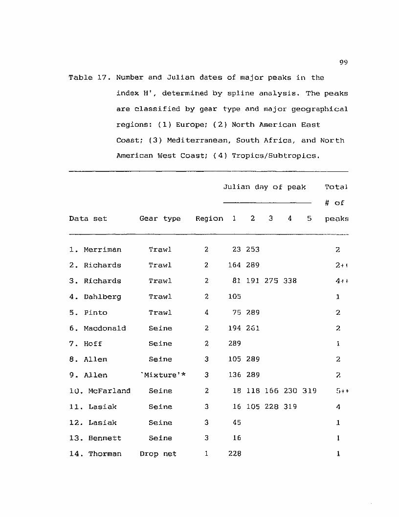
99

Table 17. Number and Julian dates of major peaks in the

index H', determined by spline analysis. The peaks

are classifi ed by gear type and major geographical

regions: (1) Europe; (2) North American East

Coast; (3) Mediterranean, South Africa, and North

American West Coast; (4) Tropics/Subtropics.

Data set Gear type

1. Merriman Trawl

2. Richards Trawl

3. Richards Trawl

4. Dahlber g Trawl

5. Pinto Trawl

6. Macdonald Seine

7. Hoff Seine

8. Allen Seine

9. Allen ' Mixture'*

10. McFa rland Seine

11. Lasiak Seine

12 . Lasiak Seine

13 . Bennett Seine

14. Thorman Drop net

Julian day of peak

Region 1 2 3 4 5

2 23 253

2 164 289

2 81 191 275 338

2 105

4 75 289

2 194 261

2 289

3 105 289

3 136 289

2 18 118 166 230 3 19

3 16 105 228 31 9

3 45

3 16

1 228

Tota l

# of

peaks

2

2 -+ 1

4 -11·

1

2

2

1

2

2

5 ++

4

1

1

1

Table 17. Continued.

15. Thorman Drop net 1 166

16. Thorman Drop net 1 166

17. Davis Flood trap 4 50

18. Sebates Bongo net 3 166

19. Pepper Scuba census 2

20. Pepper Scuba census 2 206 297

21. Cain Poison 2 99 218

22. Livingston Poison 2 136 258

+ Splines fitted with a resolution of 15 days; ++ Splines fitted with a resolution of 30 days;

All others were fitted with a resolution of 60 days. * A mixture of gears with known effort were used. The

gears included a Bag seine, Seine , Drop net, and Enclosure net.

100

1

1

1++

1

2+

2

2

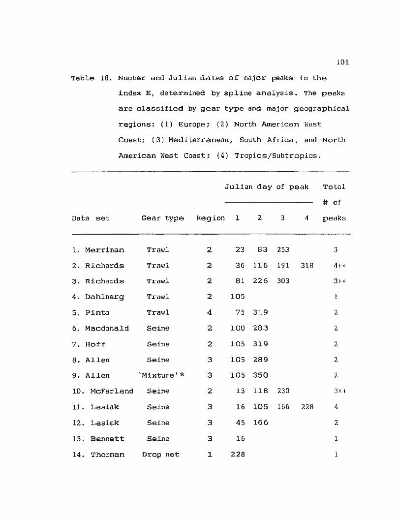
101

Table 18. Nuwber and Julian dates o£ major peaks in the

index E, determined by spline analysis. ThE~ peaks

are classified by gear type and major geographical

regions: ( 1) Europe; ( 2) North American Ettst

Coast; (3) Mediterranean, South Africa, and Nort h

American West Coast; ( 4) Tropics/Subtropics.

Data set Gear type

1. Merriman Trawl

2. Richards Trawl

3. Richards Trawl

4. Dahlberg Trawl

5. Pinto Trawl

6. Macdonald Seine

7. Hoff Seine

8. Allen Seine

9. Allen · Mixtur e'*

10. McFarland Seine

11. Lasi ak Seine

12. Lasi uk Seine

13. Bennett Seine

14. Thorman Dr op net

Julian day of peak

Region 1 2 3 4

2 23 83 253

2 36 116 191 318

2 8 1 226 303

2 105

4 75 319

2 100 283

2 105 319

3 1.05 289

3 105 350

2 13 118 230

3 16 105 166 228

3 45 166

3 16

1 228

Tot al

# o f

peal<s

3

4++

3 1+

1

2

2

2

2

2

3 1 ..

11

2

1

1

102

Table 18. continued.

15. Thorman Drop net 1 166 1

16. Thorman Drop net 1 166 1

17. Davis Flood trap 4 50 1++

18. Sebates Bongo net 3 166

19. Pepper Scuba census 2

20. Pepper Scuba census 2 129 241 341

21. Cain Poison 2 99 218

22. Livingston Poison 2 16 136 197

+ Splines fitted with a resolution of 15 days; ++ Spl i nes fitted with a resolution of 30 days;

1

3+

2

3

All others were fitted with a resolution of 60 days. * A mixture of gears with known effort were used. The

gears included a Bag seine, Seine, Drop net, a nd Enclosure net.

103

indices. Tables 13, 14, and 15 showed that two or more peaks

were more frequent in inshore and surf- zone habitats than in

other habitats. Regarding rel.ationships with gear type, there

was a similar relationship in the number of peaks with

trawling and seining (Tables 16, 17, and 18). That is, there

were two or more peaks in the three indices in an annual cycle

for data sets collected with trawls and seines but there was

no obvious pattern with any of the other gears used.

3. 5 Patterns of seasonal tracking of S with H' and E

The analysis of the type of tracking of the seasonal

patterns of S, H' and E showed two patterns: an ~in-phase'

pattern and an 'out-of-phase' pattern. The more frequent of

the two patterns is the "in-phase' pattern of tracking (Table

19). In this pattern, the major seasonal peaks and troughs in

species richness S coincided with corresponding peaks and

troughs in the heterogeneity H' and equi tabil i ty E components

of divers! ty. The second and less frequent pattern was the

"out-of-phase' pattern of tracking where the seasonal peaks

and troughs in species richness S coincided with opposite

patterns (i.e. troughs) in the heterogeneity H', and

equitability E components of diversity. This resulted in the

seasonal patterns of peaks and troughs in S to be mirror­

imaged by the corresponding peaks and troughs in H ' and E.

Figure Al (Appendix A) gives a schematic illustration of the

104

Table 19. Summary of type of seasonal tracking of the

heterogeneity H', and the equitability E,

components of diversity with respect to species

richness S. Two major patterns of this tracking

analysed from sigma-plot graphs are ·in-phase'

tracking (I.p) and ·out-of-phase' tracking (O.p)

(see text and Figure Al). Names of dominant

species associated with the major troughs in H'

Data set

1. Thorman

2. Thorman

3. Thorman

4. Pepper

5. Pepper

and E in each data set are also li.sted; names of

species for the data sets from North American East

Coast are from Scott and Scott ( 19 88).

Dorminant species

I.p O.p Family Scientific name

X Gobiidae Pomatoschistus microps

X P. microps

X P. microps

X Cottidae Myoxocephal us scorpius

X Cyclopter idae Liparis atlanticus

Stichaeidae Stichaeus punctatus

6. Macdonald X Gadidae Pollachus virens

Gasterosteidae Gasterosteus acul eatus

7. Hoff X X Atherinidae Menidia menidia

Table 19. Continued.

8. Merriman X

9. Richards X

10. Richards X

11. Cain X

12. Dahlberg X

13. Livingston X

14. McFarland X

15. Sebates x

16. Allen X

17. Allen

18. Lasiak X

19. Lasiak

20. Bennett

21. Pinto

22. Davis X

X

X

X

X

X

X

105

P leuronectidae fseudQP_le\!_t;:_Q..Q~.9t_e~

2ffi~~;i._c~rH.l.s

Ammodytidae Ammodytgs am~r_ipanus

Pleuronectidae ~· ?mericanus

Bothidae S_c;:QQ..t..b.Q.J,JH.\.1_~ aquo_sus

Pleuronectidae ~. am~.rJ~_C!!l!JS

Atherinidae Menidi2. •!!~Q_;i._giJJ.

Sciaenidae

Clupeidae

Atherinidae

Stellif~-~ J..aug_eg.l,at~s

BreVQQ~_tii? piJtro_nus

Menidia qeryl_!~n_a

Gonostomatidae Cycl_gtt:!_Qn~ l;>r_:au_eri

Engraulidae

Atherinidae

Haemulidae

Sparidae

Haemulidae

Sparidae

Atherinidae

Centropomidae

Cen tropomidae

Sea tophag i dae

AnchQQ 9.~.!...:!-g_~J;issima.

Engra_JJ_lis !nq:r;-_d_ax

~the:r;ii)Op~ a.ff;i.!1;i.S

P.9lll?..9_a_!?YS ol ~ vace!.lm

sar_p_Q §lalpa

~. oliyace_u_m

_Li t...D..Q9tl9J:_h_U_!?._ I]J_Or-!:fi.Y.rus

[\ther~_I}_i_Cl_ Qr.J!Y.:i.G~ps

AmQ_?._~~J_!:! ~.9.P_~i

b..!.llbC;i_~si_s 9.Y!:fl..!J_Qp~phalu_s

§iJ!l_enQ.t.9_Qa ~uJ,tJJ~s~_iata

106

two types of tracking.

The dominant species recorded in the original data sets

for the dates of major troughs in H' and E were also recorded

in this analysis. Generally, most of those dominant species

appeared to be species known to occur simultaneously in large

numbers or are schooling species (Table 19).

3.6 Variances and means of S, H' and E

Table 20 summarizes whether the ranks in the variances

and means of S, H' and E in different data sets showed strong,

weak, or no trend, with total number of species in the data

sets, latitude, habitat, gear type, and sampling frequency.

This summary shows that the ranks in the variances and means

of s, H' and E all showed relatively strong trends with the

total number of species in the data sets. Trends in the ranks

in the variances and means of the three indices with latitude

was, by comparison, weaker. This trend with latitude was

noticeable within regions, especially the North American East

Co8st region; it was the latitudinally most well represented

region. Habitat, sampling gear, and frequency of sampling did

not show any relationships with the ranks in the variances and

means of the three indices (Table 20).

The relative strengths of the trends in the ranks of

thevariances of the three indices with total number of species

and latitude, can be seen from Tables 21, 22 and 23. Similar

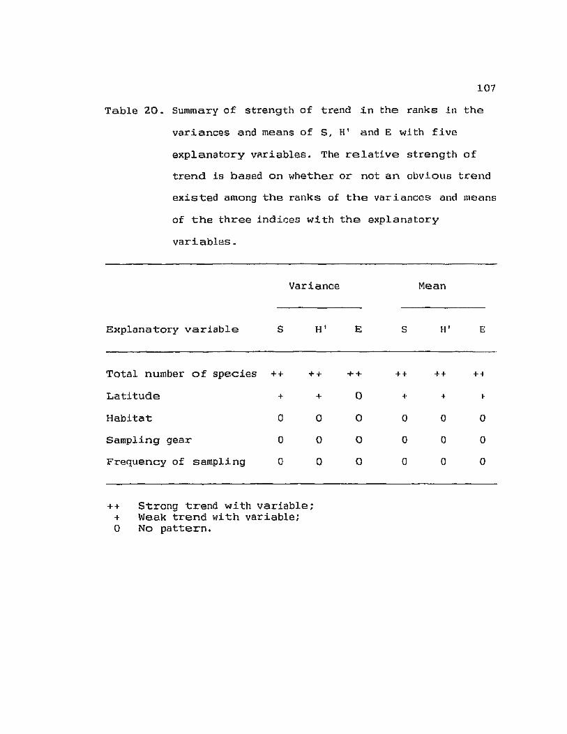
107

Table 20. Summary of strength of trend in the ranks in the

variances and means of S , H' and E with five

explanatory vnriables. The relative strength of

trend is based on whether or not an obvious trend

existed among the ranks of the variances and means

of the three indir::es wi. th the explanatory

variables.

variance

Explanatory variable S H'

Total number of species ++ ++

Latitude + +

Habitat 0 0

Sampling gear 0 0

Frequency of sampling 0 0

++ Strong trend with variable; + Weak trend with variable; 0 No pattern.

Mean

E s H'

++ ++ + +

0 + +

0 0 0

0 0 0

0 0 0

E

+-t

1-

0

0

0

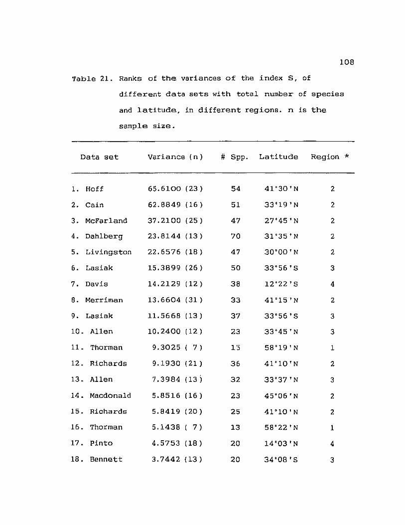
108

Table 21. Ranks of the variances of the index S, of

different data sets with total number of species

and latitude, in different regions. n is the

sample size.

Data set Variance ( n ) # Spp. Latitude Region *

1. Hoff 65.6100 ( 23) 54 41 "30 1 N 2

2. Cain 62.8849 ( 16) 51 33"19 ' N 2

3. McFarland 37 . 2100 ( 25) 47 27"45 1 N 2

4. Dahlberg 23.8144 ( 13) 70 31 "35 IN 2

5. Livingston 22.6576 ( 18) 47 30"00 IN 2

6. Lasiak 15.3899 ( 26) 50 33 "56 1 8 3

7. Davis 14.2129 ( 12) 38 12 "22 1 8 4

B. Merriman 13.6604 ( 31) 33 41 "15 1 N 2

9. Lasiak 11.5668 ( 13) 37 33"56 1 S 3

10. Allen 10.2400 ( 12) 23 33 •45 1 N 3

11. Thorman 9.3025 ( 7) 15 58"19 1 N 1

12. Richards 9.1930 ( 21) 36 41"10 1 N 2

13. Allen 7. 3984 ( 13) 32 33"37 1 N 3

14. Macdonald 5.8516 ( 16) 23 45"06 1 N 2

15. Richards 5.8419 ( 20) 25 41"10 1 N 2

16 . Thorman 5.1438 ( 7 ) 13 58 "22 1 N 1

17. Pinto 4.5753 ( 18) 20 14"03 1 N 4

18 . Bennett 3. 7442 ( 13) 20 34"08 1 8 3

Table 21. Continued.

19. Sebates

20. Pepper

21. Pepper

22. Thorman

1 . 8660 { 6 )

1.3783 {74)

1.2814 {33)

1.2388 { 7)

12

7 47"3B'N

5 47 "38' N

7

* The geographical regions numerically coded are: 1: Europe; 2: North American East Coast;

3

2

2

1

3: Mediterranean, South Africa, and North American Wesl Coast;

4: Tropics/Subtropics.

109

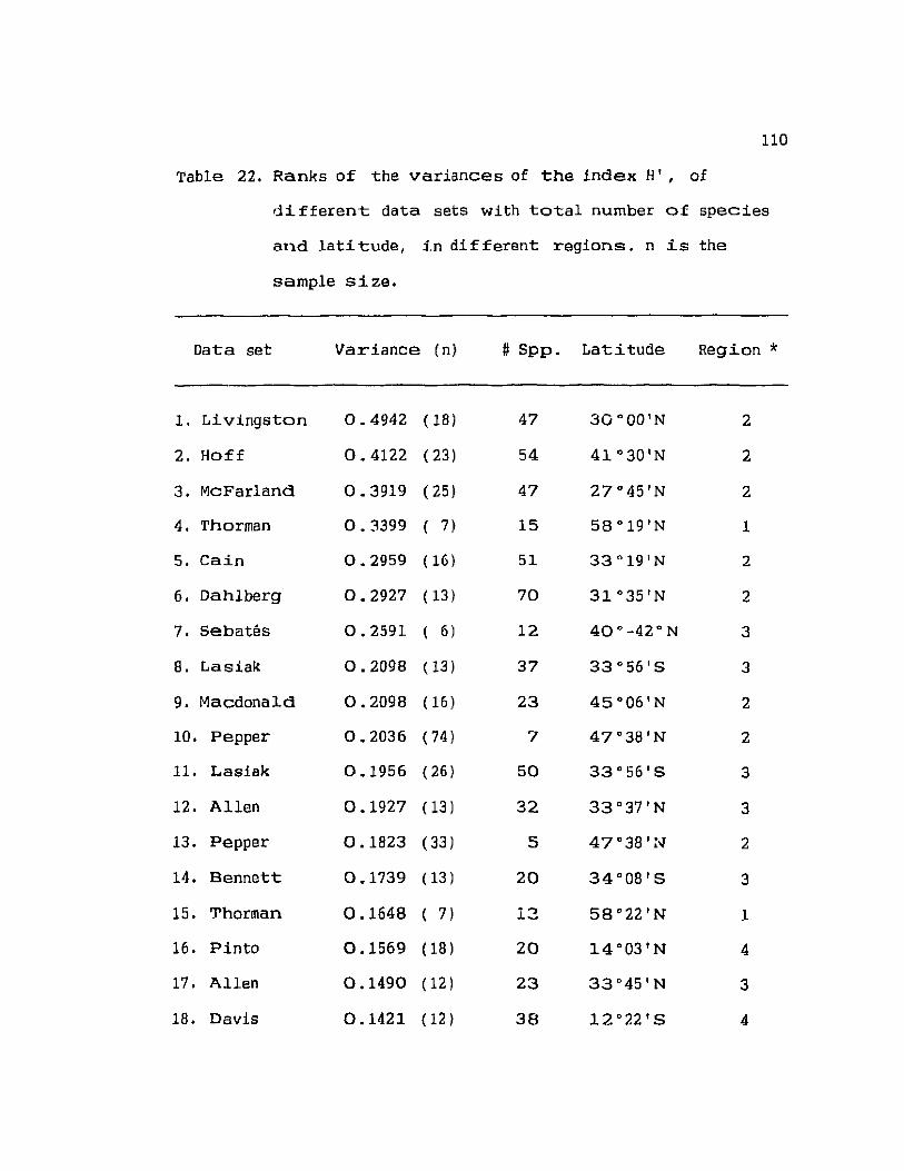
110

Table 22. Ranks of the variances of the index H' , of

d:i.. fferent data sets with total number of species

and latitude, in different regions. n is the

sample size.

Data set Variance ( n) # Spp. Latitude Region *

1. Livingston 0. 4942 ( 18) 47 30 ooO'N 2

2 . Hoff 0. 4122 ( 23) 54 41 o 30'N 2

3. McFarland 0. 3919 ( 25) 47 27 o 45' N 2

4 . Thorman 0. 3399 ( 7) 15 58°19'N 1

5. Cain 0. 2959 ( 16) 51 33°19'N 2

6 . Dahlberg 0. 2927 ( 13) 70 31 °35'N 2

7 . Sebates 0. 2591 ( 6) 12 40°-42oN 3

8. Las i ak 0. 2098 ( 13) 37 33 ° 56's 3

9. Macdonald 0. 2098 (16) 23 45 °06 'N 2

10. Pepper 0. 2036 ( 74) 7 47 °38 ' N 2

11 . Lasiak 0. 1956 (26) 50 33 ° 56's 3

12. Allen 0 .1927 (13) 32 33°37'N 3

13. Pepper 0.1823 (33) 5 47 °38 'N 2

14. Bennett 0 . 1739 ( 13) 20 34°08'S 3

15. Thorman 0 .1648 ( 7) . ..., .L ..... 58 °22' N 1

16. Pinto 0 . 1569 ( 18) 20 14 °03 'N 4

17. Allen 0 . 1490 ( 12) 23 33"45'N 3

18. Da vis 0.1421 (12) 38 12 °22 's 4

Table 22 • Continued.

19. Merriman

20 • Richards

21. Thorman

22 • Richards

0.1359 (31)

0.0782 (21)

0.0439 ( 7)

0.0381 (20)

33 41"15'N

36 41 • 10 'N

7 58"24'N

25 41 °10 'N

* The geographical regions numerically coded are: 1: Europe; 2: North American East Coast;

111

2

2

1

2

3: Mediterranean, South Africa, and North American West Coast;

4: Tropics/Subtropics.

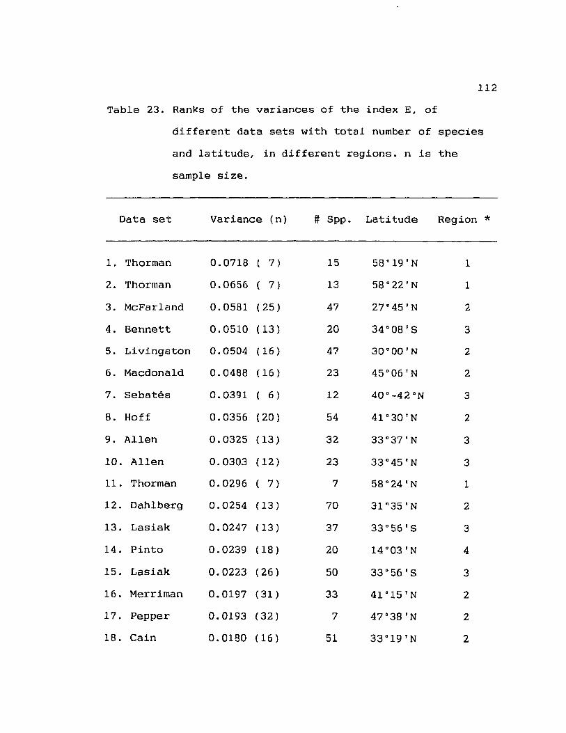
112

Table 23. Ranks of the variances of the index E, of

different data sets with total number of species

and latitude, in different regions. n is the

sample size.

Data set Variance (n) # Spp. Latitude Region *

1. Thorman 0.0718 7) 15 58°19'N 1

2. Thorman 0.0656 7) 13 58 o22'N 1

3. McFarland 0.0581 (25) 47 27°45'N 2

4. Bennett 0.0510 ( 13) 20 34"08'8 3

5. Livingston 0.0504 (16) 47 30"00'N 2

6. Macdonald 0.0488 ( 16) 23 45°06'N 2

7. Sebates 0.0391 ( 6) 12 40 °-42°N 3

8. Hoff 0.0356 (20) 54 41"30'N 2

9. Allen 0.0325 ( 13) 32 33 •37' N 3

10. Allen 0.0303 (12) 23 33"45 'N 3

11. Thorman 0.0296 ( 7) 7 58"24 'N 1

12. Dahlberg 0.0254 (13) 70 31 ~35 'N 2

13. Lasiak 0.0247 (13) 37 33"56'S 3

14. Pinto 0.0239 (18) 20 14 °03 'N 4

15. Lasiak 0.0223 (26) 50 33"56'8 3

16. Merriman 0.0197 (31) 33 41.15'N 2

17. Pepper 0.0193 (32) 7 47"38'N 2

lB. Cain 0.0180 (16) 51 33"19'N 2

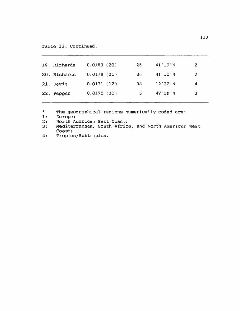
Table 23. Continued.

19 . Richards

20. Richards

21. Davis

22. Pepper

0.0180 (20)

0.0178 (21)

0.0171 (12)

0.0170 (30)

25

36

38

5

41"10'N

41"10'N

* The geographical regions numerically coded are: 1: Europe; 2: North American East Coast;

113

2

2

4

2

3: Mediterranean, South Africa, and North American West Coast;

4: Tropics/Subtropics.

114

strengths in the ranks of the means of S, H' and E wlth the

two variables can be noted from Tables 24, 25 and 26.

The ranks in the variances in S and H' were generally

higher in the data sets that recorded greater than thirty

species (Tables 21 and 22, respectively). Conversely, the

order in the ranks of the variance of E showed an inverse

relationship in this respect (Table 23). That is, the data

sets with greater than thirty species generally had lower

ranks in E. Similar patterns were observed in the ranks in the

means of S, H' and E (Tables 24, 25 and 26, respectively) with

total number of species recorded in the data sets. That is,

the ranks in the means of species richness S, and

heterogeneity H', of data sets with greater than thirty

species recorded, generally tended to be ranked higher than

those with thirty or less number of species recorded. This

pattern was again reversed in the equitability index E; the

data sets that had greater than thirty species tended to have

lower ranks in the means of E.

A relatively weaker trend in the ranks of the variances

and means in S, H' and E with latitude was observed. It was

difficult to confirm an overall latitudinal trend (i.e.

pattern among regions) in this respect. However, latitudinal

comparisons within regions, especially the North American East

Coast region, showed a pattern weaker than that shown with

numbers of species recorded in the data sets. This region is

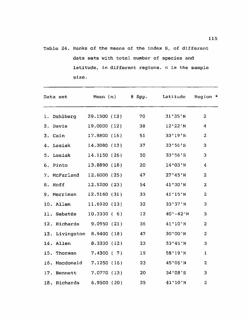
Table 24. Ranks of the means of the index 8, of different

data sets with total number of species and

latitude, in different regions. n is the sample

size.

115

Data set Mean (n) # 8pp. Latitude Region *

1. Dahlberg 29.1500 (13) 70 3l 0 35 ' N 2

2. Davis 19.0000 (12) 38 12u22 1 N 4

3. Cain 17.8800 (16) 51 33°19'N 2

4. Lasiak 14.3080 ( 13) 37 33 " 56'8 3

5. Lasiak 14.1150 ( 26) 50 33°56'8 3

6. Pinto 13.8890 (18) 20 14°03'N 4

7. McFarland 12.6000 (25) 47 27°45'N 2

8. Hoff 12.5200 (23) 54 4l 0 30'N 2

9. Merriman 12.5160 ( 31) 33 41n15'N 2

10. Allen 11.6920 (13) 32 33°37'N 3

11. sebates 10.3330 ( 6) 12 40"-42 "N 3

12. Richards 9.0950 (21) 36 41"10'N 2

13. Livingston 8.9400 (18) 47 30°00'N 2

14. Allen 8.3330 (12) 23 33a45'N 3

15. Thorman 7.4300 ( 7) 15 58 ° 19'N 1

16. Macdonald 7.1250 (16) 23 45"06'N 2

17. Bennett 7.0770 (13) 20 34°08'8 3

18. Richards 6.9500 (20) 25 41°10'N 2

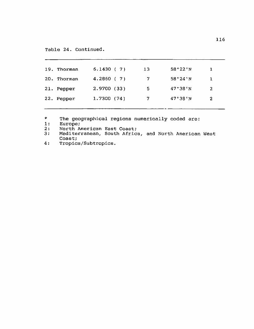
Table 24. Continued.

19. Thorman

20. Thorman

21. Pepper

22. Pepper

6.1430

4.2860

7)

7)

2.9700 (33)

1.7300 (74)

13 58°22'N

7 58°24'N

5

7

* The geographical regions numerically coded are: 1: Europe; 2: North American East Coast;

1

1

2

2

3: Mediterranean, South Africa, and North American West Coast;

4: Tropics/Subtropics.

116

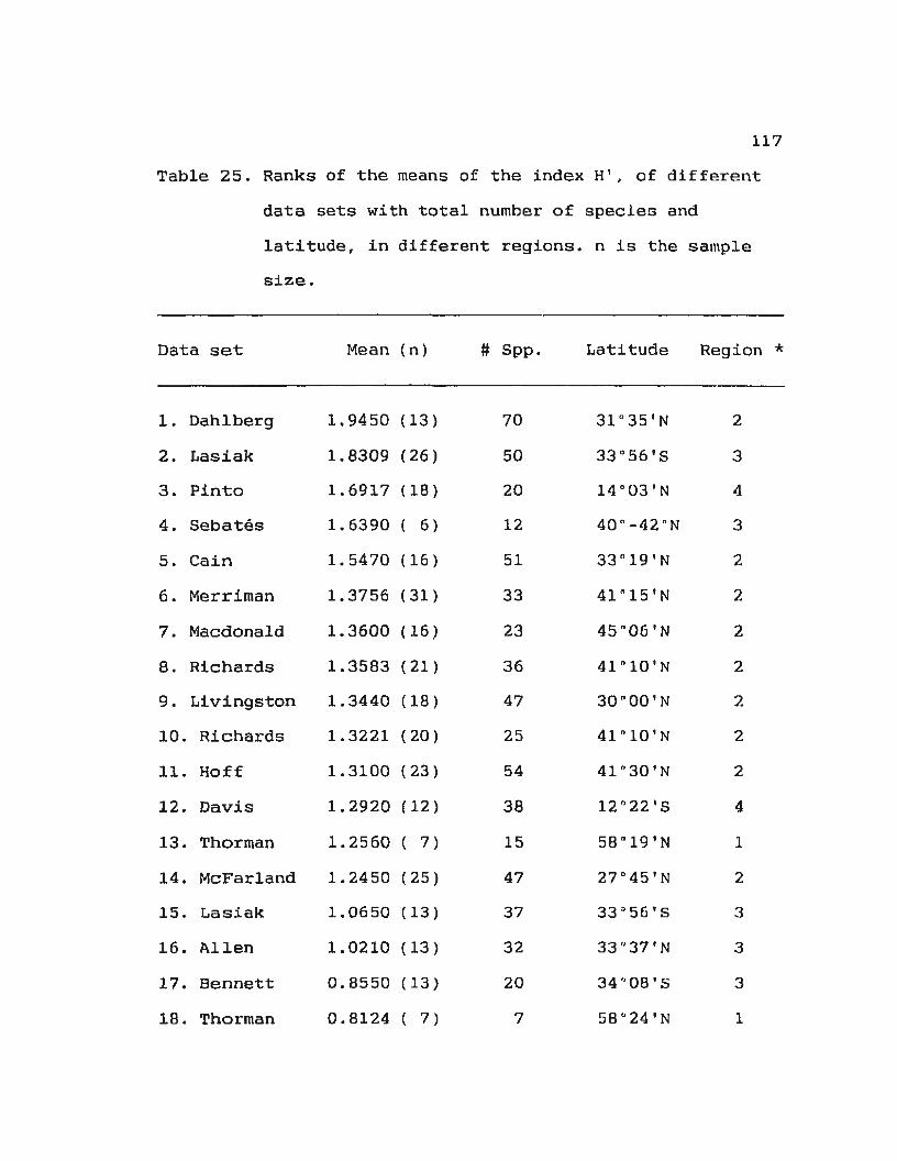
117

Table 25. Ranks of the means of the index H', of different

data sets with total number of specles and

latitude, in different regions. n is the sample

size.

Data set Mean ( n) # 5pp. Latitude Region *

1. Dahlberg 1. 9450 (13) 70 3l 0 35'N 2

2. Lasiak 1.8309 (26) 50 33 °56'5 3

3. Pinto 1. 6917 (18) 20 14°03'N 4

4. 5ebates 1.6390 ( 6) 12 4Qn-42"N 3

5. Cain 1. 5470 ( 16) 51 33°l9'N 2

6. Merriman 1.3756 (31) 33 41"15'N 2

7. Macdonald 1.3600 (16) 23 45"06'N 2

8. Richards 1. 3583 ( 21 ) 36 41"10'N 2

9. Livingston 1.3440 (18) 47 30"00'N 2

10. Richards 1. 3221 (20) 25 41"10'N 2

11. Hoff 1. 3100 ( 23} 54 41"30'N 2

12. Davis 1. 2920 (12) 38 12 "22'5 4

13. Thorman 1. 2560 ( 7) 15 58°19'N 1

14. McFarland 1. 2450 (25) 47 27°45'N 2

15. Lasiak 1 . 0650 (13) 37 33 , 56'S 3

16. Allen 1. 0210 ( 13) 32 33 "37'N 3

17. Bennett 0.8550 (13) 20 34 "08'S 3

18. Thorman 0.8124 ( 7} 7 58o24'N 1

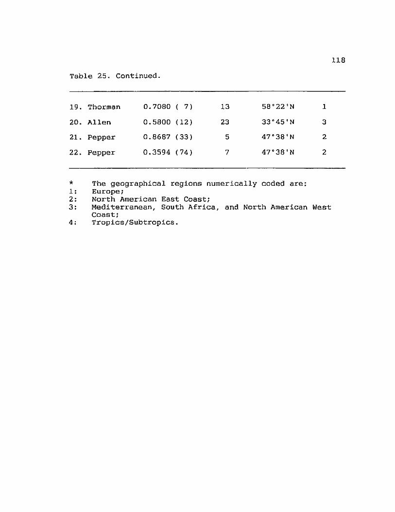
Table 25. Continued.

19. Thorman

20. Allen

21. Pepper

22. Pepper

0.7080 ( 7)

0.5800 (12)

0.8687 (33)

0.3594 (74)

13

23

5

7

* The geographical regions numerically coded are: 1: Europe; 2: North American East Coast;

1

3

2

2

3: Mediterranean, South Africa, and North American West Coast;

4: Tropics/Subtropics.

118

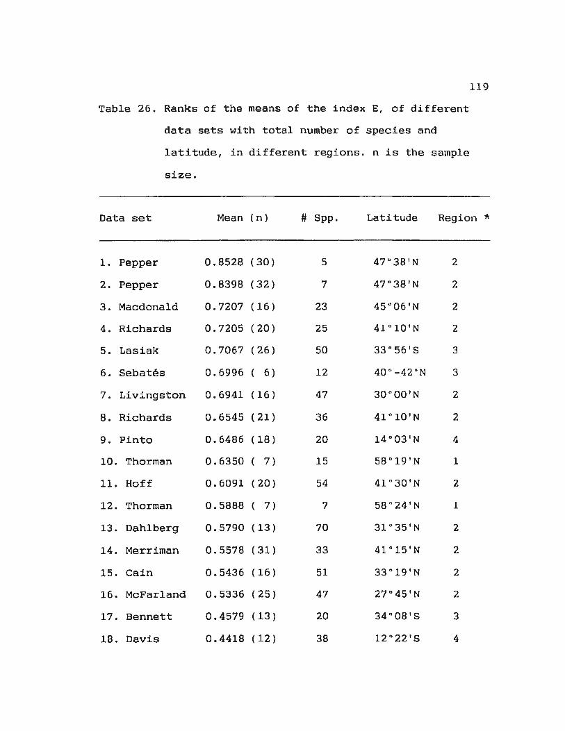
Table 26. Ranks of the means of the index E, of different

data sets with total number of species and

latitude, in different regions. n is the sample

size.

119

Data set Mean (n) # 5pp. Latitude Region *

1. Pepper 0.8528 (30) 5 47"38'N 2

2. Pepper 0.8398 (32) 7 47"38'N 2

3. Macdonald 0.7207 ( 16) 23 45"06'N 2

4. Richards 0.7205 (20) 25 4l 0 l 0'N 2

5. Lasiak 0.7067 ( 26) 50 33"56'5 3

6. 5ebates 0.6996 ( 6) 12 40o-42"N 3

7. Livingston 0.6941 (16) 47 30 " 00'N 2

8. Richards 0.6545 (21) 36 41°10'N 2

9. Pinto 0.6486 ( 18) 20 14"03'N 4

10. Thorman 0.6350 ( 7) 15 58°19'N 1

11. Hoff 0.6091 (20) 54 41"30'N 2

12. Thorman 0.5888 ( 7) 7 58"24'N 1

13. Dahlberg 0.5790 (13) 70 31 o35'N 2

14. Merriman 0.5578 ( 31) 33 41"15'N 2

15. Cain 0.5436 ( 16) 51 33"19'N 2

16. McFarland 0.5336 (25) 47 27°45'N 2

17. Bennett 0.4579 (13) 20 34 ° 08' 5 3

18. Davis 0.4418 (12) 38 12"22'5 4

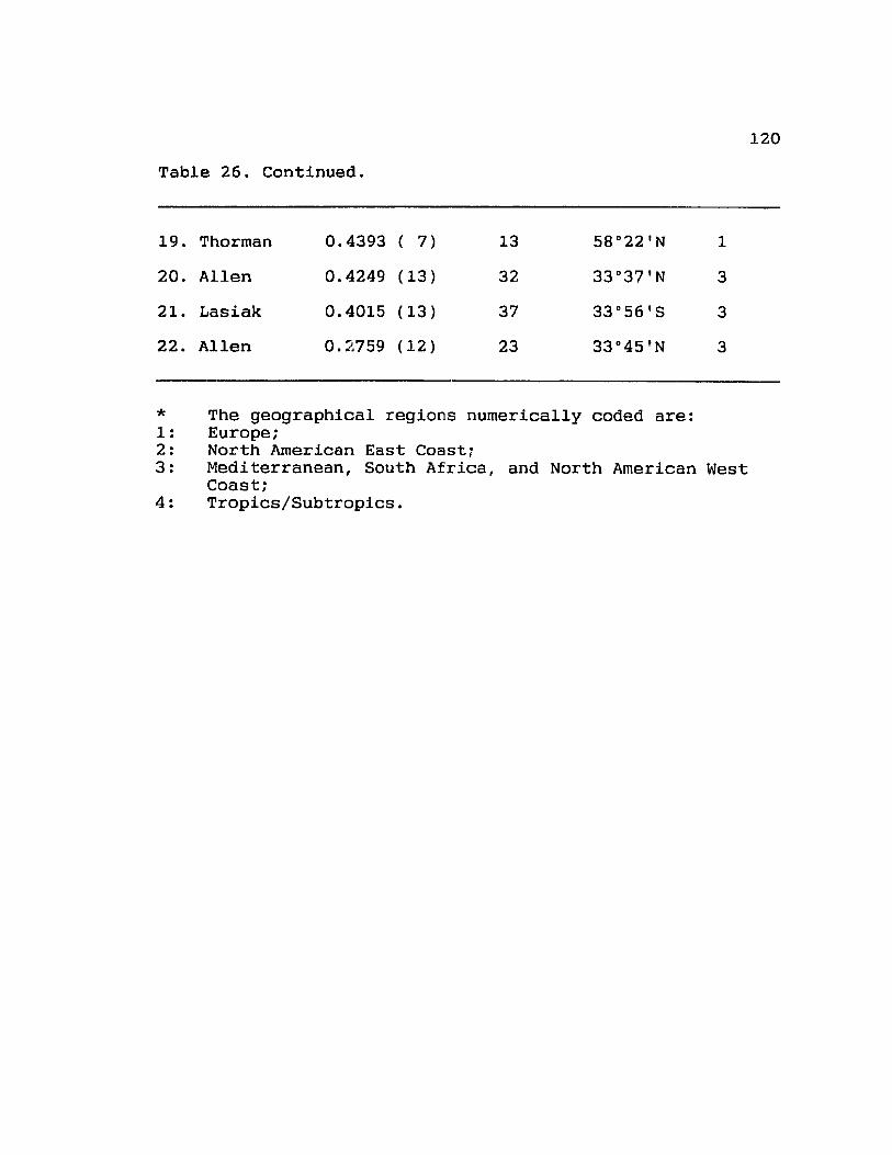
Table 26. Continued.

19. Thorman

20 . Allen

21. Lasiak

22 . Allen

0.4393 ( 7)

0 . 4249 (13)

0.4015 (13)

0.2759 (12)

13

32

37

23

* The geographical regions numerically coded are: 1: Europe; 2: North American East Coast;

1

3

3

3

3: Mediterranean, South Africa, and North American West Coast;

4: Tropics/Subtropics.

120

121

the only region for which such a comparison can be made

because the within-region latitudinal coverage is more

complete than the other three regions. There were larger

variances and means for S and H' in data sets from lower

temperate latitudes (30"N to 42"N) than at higher latitudes(>

42°N) in this region. This can be seen from Tabl~ 21 and Table

~2 for the variances and Table 24 and Table 25 for the means.

However, this latitudinal pattern was less strong in the ranks

of the variances and means for the equi tabili ty index E.

Generally, the variances for E were higher at higher temperate

latitudes (> 42"N) than at lower temperate latitudes (Table

23). The means of E from data sets collected at latitudes from

41 "N or higher in the North American East Coast region,

appeared to be ranked higher (Table 26).

3.7 Autocorrelation analysis of S, H' and E

Ranges in the minimum and maximum values for the degree

of autocorrelation (i.e. the magnitude of the regression

coefficients), the category of autocorrelation (·spiky',

·smooth', and ·mixed'), and the number of lags in each series

for S, H' and E are summarized in Tables 27, 28 and 29,

respectively. The overall ranges, minimum and maximum

respectively, for all three indices were: 10.000 to 0.6761 for

S; I 0. 000 to 0. 7341 for H': I 0. 000 to 0. 5351 for E. Of the

ranges of the autocorrelation coefficients of each index

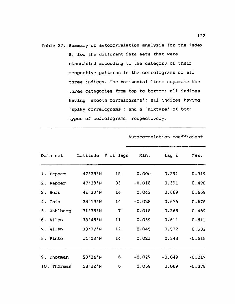
122

Table 27. Summary of autocorrelation analysis for the index

S, for the different data sets that were

classified according to the category of their

respective patterns in the correlograms of all

three indices. The horizontal lines separate the

three categories from top to bottom: all indices

having ·smooth correlograms'; all indices having

·spiky correlograms'; and a 'mixture' of both

types of correlograms, respectively.

Autocorrelation coefficient

Data set Latitude # of lags Min.

1. Pepper 47"38'N 18 o.oou

2. Pepper 47"38'N 33 -0.018

3. Hoff 41"30'N 14 0.043

4. Cain 33"19'N 14 -0.028

5. Dahlberg 31.35'N 7 -0.018

6. Allen 33.45'N 11 0.069

7. Allen 33.37'N 12 0.045

8. Pinto 14"03'N 14 0.021

9. Thorman 58"24'N 6 -0.027

10. Thorman 58"22'N 6 0.069

Lag 1

0.291

0.391

0.669

0.676

-0.265

0.611

0.532

0.348

-0.049

0.069

Max.

0.319

0.490

0. 669

0.676

0.469

0.611

0.532

-0. 515

-0.217

-0.378

Table 27. Continued.

11. Thorman 58°l9'N

12. Macdonald 45°06'N

13. Richards 41°10'N

14. Richards 41°10'N

15. Lasiak 33°56'8

16. Lasiak 33"56'S

17. Davis 12°22'8

18. Merriman

19. Livingston 30°00'N

20. McFarland 27°45'N

21. Bennett 34°08'8

6

5

14

14

12

15

11

14

14

14

12

0.070

-0.152

0.012

0.008

0.048

-0.002

0.000

0.033

-0.002

-0.015

-0.040

0.148

-0.305

0.078

0.072

0.059

-0.011

-0.564

0.504

0.352

0.672

0.615

123

-0 .358

0.438

-0.388

-0.284

-0.337

-0.192

-0.564

0.504

-0.391

0.672

0.615

124

Table 28. Summary of autocorrelation analysis for the index

H', for the different data sets that were

classified accordi ng to the category of their

respective patterns in the correlograms of all

three indices. The horizontal lines separate the

categories from top to bottom: all indices having

·smooth correlograms'; all indices having 'spiky

correlograms'; a 'mixture' of both types of

correlograms, respectively.

Data set

1. Pepper

2. Pepper

3. Hoff

4. Cain

5. Dahlberg

6. Allen

7. Allen

8. Pinto

9. Thorman

10. Thorman

Latitude # of lags

47D38'N

47°38'N

41D30'N

33°19'N

31°35'N

33D45 ' N

33°37 ' N

14D03 ' N

18

33

14

14

7

11

12

14

6

6

Autocorrelation coefficient

Min.

-0.010

0.031

0.031

-0.025

-0.006

-0.027

-0.036

0.019

-0.063

0.009

Lag 1

0.236

0.232

0.479

0.734

0.449

0.291

0.410

0.333

- 0 . 646

0.009

Max.

0.370

0.459

0.479

0.734

-0.449

-0.358

0.410

-0.378

-0.646

- 0.395

Table 28. Continued.

11. Thorman 58°19'N

12. Macdonald 45°06'N

13. Richards 41°10'N

14. Richards 41°10'N

15. Lasiak 33"56'S

16. Lasiak 33"56'5

17. Davis !2°22'S

18. Merriman

19. Livingston 30°00'N

20. McFarland 27°45'N

21. Bennett 34"08'S

6

5

14

14

12

15

11

14

14

14

12

-0.033

0.006

-0.004

-0.062

0.000

0.002

-0.008

-0.013

0.005

0.015

- 0.011

-0.182

0.006

-0.030

0.104

0. 287

-0.384

-0.079

0. 186

0.209

-0.097

-0.049

125

-0.567

-0.375

0.230

0.277

-0.436

0.401

0.290

-0.244

-0.292

0.365

0.243

126

Table 29. Summary of autocorrelation analysis for the index

E, for the different data sets that were

classified according to the category of their

respective patterns in the correlograms of all

three indices. The horizontal lines separate the

categories from top to bottom: all indices having

'smooth correlograms'; all indices having 'spiky

correlograms'; a "mixture' of both types of

correlograms, respectively.

Data set

1. Pepper

2. Pepper

3. Hoff

4. Cain

5. Dahlberg

6. Allen

7. Allen

B. Pinto

9. Thorman

10. Thorman

Autocorrelation coefficient

Latiude # of lags Min.

47"38'N 18

47•38'N 33

41.30'N 14

33"19'N 14 -0.010

31°35'N 7 -0.027

33"45'N 11 0.032

33"37'N 12 -0.033

14"03'N 14 0.003

58"24'N 6 -0.036

58"22'N 6 0.039

Lag 1

0.362

0.493

0.150

0.402

0.376

-0.535

0.215

Max.

-0.365

0.493

-0.435

0.402

-0.390

-0.535

-0.315

Table 29. Continued.

11. Thorman 58°19'N 6

12. Macdonald 45°06'N 5

13. Richards 41°10'N 14

14. Richards 41°10'N 14

15. Lasiak 33°56'8 12

16. Lasiak 33°56'8 15

17. Davis 12°22'5 11

18. Merriman 14

19. Livingston 30°00'N 14

20. McFarland 27°45'N

21. Bennett 34°08'8

14

12

0.030

0.043

-0.031

0.021

0.003

0.020

0.001

-0.022

0.001

0.018

-0.195

0.225

-0.283

-0.309

0. 295

-0.302

0.033

0.266

0. 065

-0. 058

127

0.223

-0.355

-0.283

-0. 40'1

-0. 48 .1.

-0.250

-0.292

-0.417

-0.233

-0.210

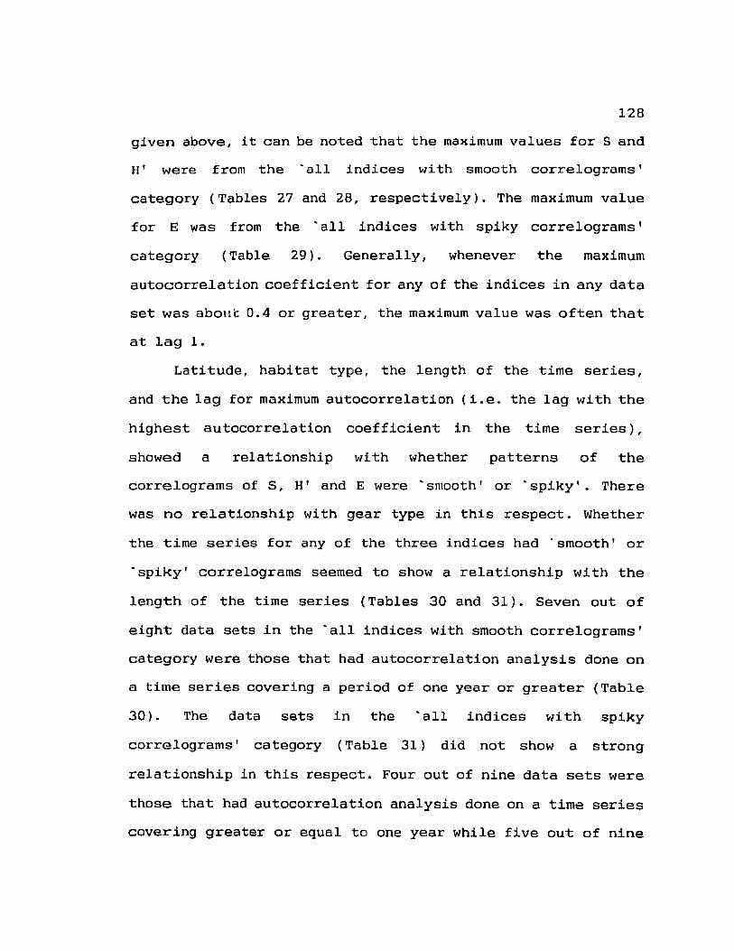
128

given above, it can be noted that the maximum values for S and

H' were from the ·all indices with smooth correlograms'

category {Tables 27 and 28, respectively). The maximum value

for E was from the ·all indices with spiky correlograms'

category (Table 29). Generally, whenever the maximum

autocorrelation coefficient for any of the indices in any data

set was aboBi: 0.4 or greater, the maximum value was often that

at lag 1.

Latitude, habitat type, the length of the time series,

and the lag for maximum autocorrelation (i.e. the lag with the

highest autocorrelation coefficient in the time series),

showed a relationship with whether patterns of the

correlograms of S, H' and E were ·smooth' or 'spiky'. There

was no relationship with gear type in this respect. Whether

the time series for any of the three indices had ·smooth' or

'spiky' correlograms seemed to show a relationship with the

length of the time series (Tables 30 and 31). Seven out of

eight data sets in the 'all indices with smooth correlograms'

category were those that had autocorrelation analysis done on

a time series covering a period of one year or greater (Table

30). The data sets in the 'all indices with spiky

correlograms' category (Table 31) did not show a strong

relationship in this respect. Four out of nine data sets were

those that had autocorrelation analysis done on a time series

covering greater or equal to one year while five out of nine

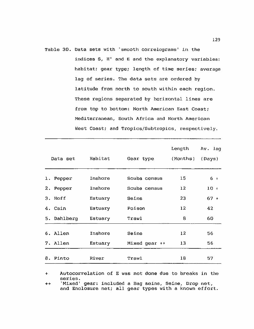
129

Table 30. Data sets with "smooth correlograms' in the

indices 5, H' and E and the explanatory variables:

habitat; gear type; length of time series; average

lag of series. The data sets are ordered by

latitude from north to south wi thin each reg i on.

These regions separated by horizontal lines are

from top to bottom: North American East Coast ;

Mediterranean, South Africa and North American

West Coast; and Tropics/Subtropics, respectively.

Lengt h Av. l.ag

Data set Habitat Gear type (Months) (Days)

1. Pepper Inshore Scuba census 15 6 • 2. Pepper Inshore Scuba census 12 10 ~

3. Hoff Estuary Seine 23 67 +

4. Cain Estuary Poison 12 42

5. Dahlberg Estuary Trawl 8 60

6. Allen Inshore Seine 12 56

7. Allen Estuary Mixe d gea r ++ 13 56

8. Pinto River Trawl 18 57

+ Autocorrelation of E was not done due t o breaks in t he series.

++ "Mixed' gear: i ncluded a Bag seine, Seine, Dr op net, and Enclosure net; all gear types with a known effort.

130

Table 31. Data sets with 'spiky correlograms' in the indices

s, H' and E and the explanatory variables:

habitat; gear type; length of time series; average

lag of series. The data sets are ordered by

latitude from north to south within each region.

These regions separated by horizontal lines are

from top to bottom: Europe; North American East

coast; Mediterranean, south Africa, and North

American West Coast; Tropics/Subtropics,

respectively.

Data set Habitat Gear type

Length

(Months)

Av. lag

(Days)

1. Thorman River Drop net 7 53

2. Thorman Estuary Drop net 7 53

3. Thorman Estuary Drop net 7 53

4. Macdonald Inshore Seine 6 70

5. Richards Inshore Trawl 13 35

6. Richards Inshore Trawl 13 37

7. Lasiak Surf-zone Seine 13 56

8. Lasiak Surf-zone Seine 26 59

9. Davis Estuary Flood trap 6 27

131

data sets were those covering a time series of less than one

year (Table 31). Whether a data set had both types of

correlograms among the three indices, where any two indices

may have either ·smooth' or ·spiky' correlograms, seemed to be

related to habitat. That is, the data sets in the 'mixed '

category were data collected either in a surf-zone or an

estuarine marsh habitat (Table 32) . Two other surf -zone data

sets were included in the ·all indices with spi!<y

correlograms ' category (Table 31).

The lag with the maximum autocorrelation in all data sets

with ·smooth correlograms' in S, H' and E showed a

relationship with latitude (Table 33). Apparently the lags

with maximum autocorrelation are between five t o six months

after, in the time series at higher latitudes for all three

indices. At lower latitudes the lag with the maximum

autocorrelation is often less than five months (Table 33).

3.8 Summary of results

1. Differential catchabili ty of species d i d not n ffec t

the seasonal pattern of diversity if catchability was constan t

within a study.

2. Visual and spline analysis showed that there was no

latitudinal difference in the number of annual peaks in

species richness S, heterogeneity H' and equitability E within

the North American East Coast region. Although the number of

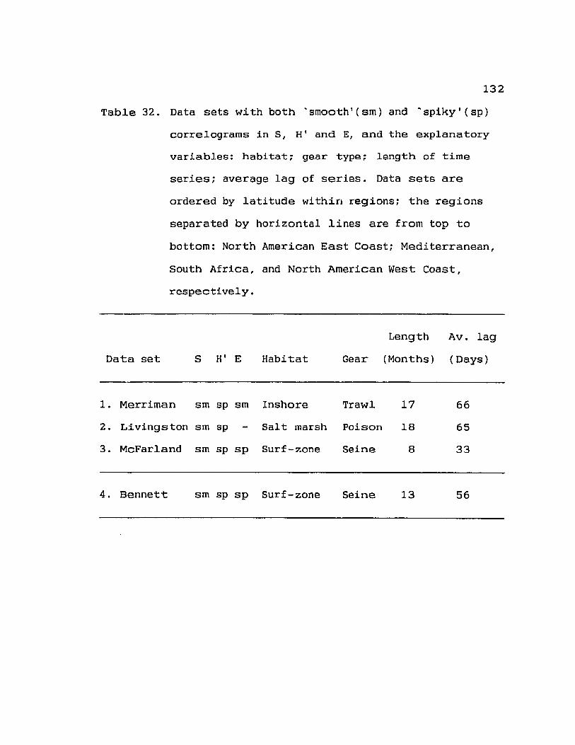
132

Table 32. Data sets with both ·smooth' ( sm) and ~spiky' { sp)

correlograms in S, H' and E, and the explanatory

variables: habitat; gear type; length of time

series; average lag of series. Data sets are

ordered by latitude within regions; the regions

separated by horizontal lines are from top to

bottom: North American East Coast; Mediterranean,

South Africa, and North American West Coast,

respectively.

Data set s H' E Habitat Gear

1. Merriman sm sp sm Inshore Trawl

2. Livingston sm sp Salt marsh Poison

3. McFarland sm sp sp Surf-zone Seine

4. Bennett sm sp sp Surf-zone Seine

Length

(Months)

17

18

8

13

Av. lag

(Days)

66

65

33

56

133

Table 33. Latitudinal trend in the time lag of maximum

autocorrelation of pattern in S, H' and E for data

sets with "smooth correlograms'. · The time (t) at

maximum lag is in months.

Data set

1. Pepper

2. Pepper

3. Hoff

4. Merriman

5. Allen

6. Allen

7. Cain

8. Dahlberg

9. Livingston

10. McFar land

11 . Pinto

12. Bennett

1. Pepper

2. Hoff

3. Allen

Latitude

47°38'N

47°38 1 N

41°30 1 N

41°15 IN

33°45'N

33 °37 1 N

33 °19 IN

31°35 1 N

30° 00 IN

27°45 1 N

l4°03 1 N

34°08'8

47°38 1 N

41°30 1 N

33°45'N

Index

s

s

s

s

s

s

s

s

s

s

s

s

HI

HI

H'

Autocorrel. coeffs.

Lag 1

0.291

0.391

0.669

0.504

0.661

0.532

0.676

-0.265

0.352

0.672

0.352

0.61 5

0.232

0.479

0.291

Max. t

0.319 0.75

0.464 0.50

-0.544 6

-0.466 6

-0.576 5

-0.473 5

0.610 1

0.469 3

-0.39 1 8

0.61 7 1

-0. 5 1 5 3

- 0.52 5 5

0. 4 59 0.50

0.401 12

-0.358 7

Table 33. Continued.

4. Allen

5. Cain

6. Dahlberg

7. Pinto

1. Merriman

2. Allen

3. Allen

4. Cain

5. Dahlberg

6. Pinto

33"37 1 N

33" 19 IN

31 "35 1 N

14"03'N

41"10'N

33"45 IN

33" 37 IN

33" 19 IN

31"35'N

14"03 'N

HI

HI

HI

H'

E

E

E

E

E

E

0.410

o. 734

0.449

0.333

0.266

0.150

0.402

0.362

0.493

0.376

-0.230

-0.577

-0.437

-0.378

-0.417

-0.435

-0.202

-0.365

-0.430

-0.390

8

3

4

14

5

7

4

1

4

14

134

135

annual peaks were variable in this region, two peaks within an

annual cycle was found to be common by both analyses. That is

all data sets had at least two peaks within an annual cycle.

The time interval between the first and second peak for the

eleven data sets from this region was five months on average.

On the other hand, the analysis for time of occurrence of

seasonal peaks in S, H' and E showed a relationship with

latitude within the North American East Coast region. '!'hat is,

the peaks within an annual cycle occurred earlier at lower

latitudes (:5 4l 0 15'N) and later at higher latitudes (>

4l 0 l5'N). Regression analysisof this latitudinal trend in the

time of occurrence of the first peak for all the dL~tu sets

from this region was stronger in heterogeneity II' and

equi tabili ty E, than in species richness s.

3. Analysis of peaks and troughs showed that there were

two major patterns of seasonal tracking of specjes richness S

by heterogeneity H' and equitability E in marine fish

communities; an "in-phase' pattern is one, an ·out-of-phase'

pattern is another. In-phase changes in S, H' and E occur more

than the out-of-phase pattern.

4. Seasonal variability inS, H' or E was not related to

geographical region, habitat type, sampling gear and frequency

of sampling (Table 20).

5. The seasonal variability in the three indi.ces measured

by the means and variances was related to species richness S

136

of individual data sets (Table 20). Variances and means in

species richness S (Tables 21 and 24) and heterogeneity

H 1 (Tables 22 and 25) tended to be higher in data sets with

more. species and lower in data sets with fewer species. On the

other hand, the variance and mean of equi tabili ty E (Tables 23

and 26) showed an opposite pattern in this respect. There was

also some relationship with latitude within the North American

East Coast region.

6. Results of autocorrelation analysis showed that, in

data sets with ~smooth correlograms' , the lag of maximum

autocorrelation for S, H 1 and E was longer at latitudes ~

33" 37 1 N than at latitudes < 33 • 37 1 N. In higher latitudes it

\oJas five months or greater; this length of time was generally

shorter than five months at latitudes < 33 a 37 IN.

4 DISCUSSION

4.1 Data sets used in this study

The principal objective of this study was to use

available research fish catch data, collected over time, to

discover and describe seasonal patterns of diversity in fish

communi ties. Such research requires large sui table databases:

the data have to be quantitative and collected by consistent

sampling procedures. Twenty-two data sets which fulfilled

these conditions were compiled for use in this study. Eleven

of these data sets were from the North American East Coast

region, making this region the best represented reg.ion in the

study. This enabled within study as well as among study

comparisions of seasonal patterns of diversity to be made for

this region.

The limitation in terms of global and regional coverage

reflects firstly historical and current research interests in

the subject in different regions. Secondly, the small number

of data sets compiled for this study is the rosul t of

inaccessibility of any available data as well as the

unsuitability of data based on the above criteria. 'fhal ts,

for inclusion the data sets have to be collected by clearly

specified sampling gear( s), the sampling procedures have to be

accurately described and the taxonomic information of speci.cs

caught had to be complete to species level.

138

4.2 Effect of bias by sampling gears

A wide range of fishing gears for large scale commercial

purposes are described in FAO (1978) and Strange (1981).

Rounsefell ( 1975) provided descriptions and illustrations of

a fairly complete range of fishing gears. He: classified these

range of gears according to types of species which can be

suitably captured with particular gear types as well as the

types of habitats in which the gears are suitable for use.

Often ecological or fisheries researchers rely on modified and

appropriately adapted miniature versions of such fishing gears

to obtain samples for studying biological and ecological

aspects of fish.

Different sampling gears have different efficiencies in

catchability (Taylor, 1953; Kenchington, 1980; Byrne et al.,

1981; Gulland, 1983). Gears such as seines, traps set for

migrating species, electrofishing and poisoning with compounds

such as rotenone are more complete (Huntsman, 1948); their

efficiency can be increased with repeated usage in a set area.

On the other hand, gears such as trawls (Taylor, 1953; Kjelson

and Johnson, 1978; Gibbs and Mathews, 1982; Engas and God¢,

1989(a, b)) and gillnets (Hamley, 1975) are less complete. It

is known that regardless of the type of gear or design, the

existence of a certain degree of bias in any research sampling

protocol is inevitable (Byrne et al. , 1981 ) . Therefore, any

research sampling design should aim to eliminate or control

139

any bias as much as possible. One has to take into account the

possible biases of the sampling gear( s) and any underlying

assumptions of the design of the

interpreting the data (Byrne ~-.t

Sissenwine, 1983).

sampling procedure(s) in

al_., 1981; Collie and

Because research catch data available from published

sources were used to study seasonal patterns of diversity of

fish communities in this study, it was necessary to assess if

biases in sampling affected seasonal patterns of divcrsi ty

discerned from the data. The results of the simulation using

the "approximate randomization test" procedure (Noreen, 1989)

showed that as long as any bias that existed within studies

was constant, it does not affect the seasonal patterns of

diversity discerned from the data in relative terms. FJgures

2 and 4, and Figures 3 and 5 demonstrate this conclusion for

the heterogeneity H' and equi tabili ty E components of

diversity, respectively.

As demonstrated by the above simulation analysis, as long

as biases were constant within each study, conclusions from

any comparisions of seasonal patterns of diversity among

studies should be valid. Furthermore, most of the data sets

used in this study were collected largely in similar habitats

(inshore and estuary) and by related sdmpling gears ( traHling

and seining) (Table B2, Appendix B), using sampling designs

planned for research purposes. Problems of gear selectivi. ty

140

and amonq-study biases 1r1ere carefully guarded against by

screening and selecting the data sets, based on the efficiency

and consistency of the design of the sampling protocol (see

section 2.1). Although sampling biases may not be perfectly

controlled in this manner, such considerations would minimize

its effects and that of any interaction among latitude,

habitat and gear type, enabling true patterns due to these

variables to be exposed.

The among-study comparisions

variances and means of the indices

of the ranks in the

can also be argued to

suffer from variabilities due to biases in sampling gear among

studies because of problems discussed in Green (1979, pp. 32-

35). However, my results consistently showed strong trends in

the ranks in all indices with the total number of species

recorded in each study (Table 20). There was no trend

associated with gear. Hence, I conclude that the influences of

any biases in gear on the variability in the variances and

means in the indices among studies are relatively negligible,

at least at the spatial scales involved in this comparative

study (Figure 1), than that due to the influence of species

numbers.

With respect to gear selectivity, it is also necessary to

clarify here that the term ·fish community' used in the text

in the context of this study, refers specifically to species

of a certain size range and to individuals of certain size

141

ranges of particular species which, as a result of their size

and behaviour, are susceptible to the sampling gear used.

Therefore, -fish community', as used in this context, does not

represent truely natural communities; I define a natural fish

community to be one that comprises of all individuals of the

different species that coe>:ist and interact within a def lncd

geographical area.

4.3 Seasonal patterns of diversity in fish communities

Fish communi ties from the North American East Coust:

generally tended to have two peaks in species richness S,

heterogeneity H', and equitability E over an annual cycle at

latitudes > 41 a 10 'N and two to three peaks at latitudes $

41°10'N. However, two annual peaks in the three indices is the

most common pattern (Figures 9, 10, and 11 ) . 'I'hc peaks,

indicating an influx of species into the communi ties, are

separated by troughs which indicate an efflux, respectively.

Consequently, seasonal patterns of peaks and troughs appear in

the three indices, which are either "in-phase' or "out-of­

phase' (Figure Al, Appendix A).

It has been calculated from Julian dates that the time

interval between the two peaks, or that of the first two peaks

in data sets with more than two peaks, \'laS five months on

average. Of the 22 data sets analysed, the index S from data

sets from higher temperate latitudes (> 33o north or south)

142

that had ·smooth correlograms' appeared to have a time

interval of five or six months between lag 1 and the lag of

maximum autocorrelation (Table 33). This indicates that there

is a better chance of predicting the seasonal pattern of any

of the three indices five or six months later at higher

latitudes. An interval of such magnitude coincides with the

time interval between spring and fall peaks in primary

production in temperate latitudes as proposed by the "match­

mismatch" hypothesis (Cushing, 1967; 1975; 1990). Several

examples using autocorrelation techniques to analyse temporal

and spatial cycles in ecological data have been reviewed

(Platt and Denman, 1975). They stated that spectral analysis

using autocorrelation techniques is a relevant method of

verifying any predictions in the periodicity of such cycles.

The results of the spline analysis (Figures 9, 10, and

11) show that the number of peaks inS, H' and E within an

annual cycle fall into two main clusters in the North American

East Coast region; one cluster is more a warm-months cluster

while the other is a cold-months cluster. This implies that

there are two major events of influx and efflux of species

within an annual cycle in this region; one is associated with

the warming of the sea during early spring into late summer

while the other is associated with its cooling during early

fall till late winter.

As reviewed in the introduction, many studies on seasonal

143

patterns of diversity in fish communities have reported peaks

and troughs in species richness S, heterogeneity H' and

equitability E to be associated with warm and cold seasons of

the year. Species richness S was reported to be low in colder

months of the year and high during the warmer months

(McFarland, 1963; Richards, 1963; Shuntov, 1971; Oviatt and

Nixon, 1973; Hoff and Ibara, 1977; Warburton, 1978; Quinn,

1980; Rainer, 1984; Thorman, 1986). Unlike species richness s,

the heterogeneity component of diversity H' was found to be

high during both the colder and warmer seasons of the yeur.

Species heterogeneity H' was reported to be high during t he

warmer seasons of the year by a number of studies (Oviatt and

Nix()n, 1973; Subrahmanyam and Drake, 1975; Allen and Ho r n,

1975; Warburton, 1978; Al-Daham and Yousif, 1990). On the

other hand, some studies reported this index to be high during

the colder seasons of the year (Hoff and I b a ra, 1977; Allen,

1982; Claridge et al., 1986). Similarly, the equ i tabi. .Uty

index of diversity E was also reported to have maximum values

during both the warmer (Dahlberg and Odum, 1970; War burton,

1978; Al-Daham and Yousif , 1990) and colder seasons of the

year (Claridge et al., 1986).

Therefore, it can be concluded that the seasonal changes

in patterns of diversity in fish communities, as descri bed

above, are associated with major influxes and effluxes of

species into and out of those respective communi ties. My

144

analysis of the major seasonal "troughs' in H' and E from the

22 data sets used in this study showed that the 'troughs' were

associated with the influx into the different communities by

dominant species. This was also observed from a study of small

flatfishes and other demersal fishes at seven stations inshore

of Heceta Bank, Oregon (Pearcy, 1978). A decline in the

heterogeneity index H' in Pearcy's study was found to be

associated with the predominance in the catch (86% by number)

by the Pacific sanddab, Ci tharichthys sordidus, a dominant

species in inshore ( 74-102 m) waters. In this regard, the

species associated with the major 'troughs' observed in the

data sets used in my study are recorded in Table 19, many of

them are either schooling species or those that have some form

of aggregating behaviour.

When a species with an aggregating behaviour, or one that

is numerically dominant in a community occurs, there is a

proportionately greater contribution to the total numbers of

fish in the community by this species. However, there is no

corresponding increase in S with increase in total numbers.

Consequently, the hetergeneity (H') and equitabllity (E)

indices drop, resulting in the occurrence of 'troughs' in

these two indices, and an ·out-of-phase' pattern in the

overall seasonal pattern of diversity. However, when the

fluxes are equitable for all species, the overall seasonal

pattern would be 'in-phase' {Figure Al, Appendix A).

145

4.4 Processes regulating seasonal patterns of diversity

The seasonal influx and efflux of fish species that is

responsible for the two major peaks in the indices S, H' and

E observed in data sets from the North American East Coast

region, can be due to a number of processes. Some idea of what

these processes are can be attained by thinking of variables

and factors that are known to influence and regulate fish

populations on a seasonal basis. In studies on fish population

dynamics it is known that the number of fish at a given time

in a given area is the result of an integration of the

influences of both abiotic (environmental) and biotic

variables. Abiotic variables include temperature, light and

motion (water circulation and currents) ( Skud, 1982;

Longhurst, 1984; Rothschild, 1986). Cushing (1982) discussed

some of these factors under the general topic "climate" and

how it influences marine fisheries production. Biotic

variables include fecundity, growth, age at maturi ·ty

(Rothschild, 1986; Daan et al., 1990; Rijnsdorp ~~ ~l_.l_ ., 1991),

larval nutrition and larval predation (Longhurst, 1984;

Rothschild, 1986; Pepin, 1990). Besides these, anthropogenic

factors such as impact from fishing and water pollution also

influence fish population dynamics (Rothschild, 1986). Because

of the complexity of the relationships among these variables

and their influences on fish population dynamics, the

separation of the effects of fishing from that of any of the

other factors has been difficult for exploited

populations (Rothschild, 1986; Daan et al., 1990).

146

fish

In this study, I have collated time series data on fish

catches from which the indices S, H' and E were calculated, as

well as data on habitats sampled and gear used. Based on the

patterns shown by my analyses of these data, as well as

published information, I propose the following processes to be

possible contributors to the observed seasonal patterns of

diversity in fish communi ties of the North American East Coast

region. The proposed processes would serve as starting points

from which to investigate accurately which of them are

involved, by collecting further data on variables such as

reproductive condition, age composition, diet, body condition,

as well as direct measurements of physical variables such as

sea temperature and motion. This will allow one to integrate

and identify accurately what processes are responsible for the

observed patterns.

4.4.1 Recruitment variability

Seasonal reproductive and recruitment patterns (i.e.

recruitment variability) (Longhurst, 1984) of different

species of fish can influence the seasonal patterns of

diversity in fish communi ties as analysed in this study.

Ricker (1975) defines recruitment as the addition of new fish

to the vulnerable population by growth from among smaller size

147

categories. "Vulnerable population" in this context implies

the size classes of fish in the population that are

susceptible to capture by any appropriate fishing gear. A

definition of recruitment more specific to fisheries

scientists is "adding a new cohort of individuals to an

exploitable stock", rather than to a biologically defined

population (Holt, 1990). On the other hand, a definition more

sui tabla to ecology is the addition of a cohort of young

individuals to a population (Sale, 1990). Ricker's definition,

which is intermediate between that by Holt and Sale and too

that it is appropriate to the context of this study, will be

implied throughout the text where no further clarification is

given.

In temperate latitudes, physical factors such as

temperature and photoperiod undergo apparent sensonal

variations in their magnitudes, being lowest and shortest in

winter and highest and longest in summer, respectively . These

variations provide external cues for the timing of seasonal

reproductive activity in many temperate species of fish (Fry ,

1971; DeVlaming, 1972, 1975; Lam, 1983) to coincide with

seasons which can potentially enhance recruitment through

increased larval and juvenile food, their survivorship and

dispersal.

The regulation of reproductive activity by temperature

and photoperiod has been observed in both freshwater and

148

marine fishes. DeV1aming (1972) critically reviewed the effect

of these two environmental factors in controlling teleost

reproductive cycles in six major orders. It was reported in

the green sunfish, Lepomis cyanellus (Kaya, 1973), the

cyprinid, Notemigonus crysoleucas (DeVlaming, 1975), and the

pumpkinseed, Lepomis gibbosus (Burns, 1976). Data from Colton

~t ?1. (1979) and Sherman et al. (1984; 1987) showed spawning

seasons in many marine fishes from the North American East

Coast to be occurring either during the 'cold months'(October­

March) or the ·warm months'(April-September) of the year. From

their data from Georges Bank and the Middle Atlantic Bight the

·cold months 1 spawners included examples such as: Gadidae­

Gi:!_du§. morhua, Pollachius virens, Melanogrammus aeqlefinus;

Clupeidae- Clupea harengus; Ammodytes sp .. Examples of the

warm months 1 spawners included: Gadidae- Merluccius

bilinearis, Urophyscis spp.; Scombridae- Scomber scombrus;

Labridae- Tautogolabrus adspersus (this species undergoes

torpor during the 'cold months').

The influence of such cues on the reproductive cycles of

marine fishes is important , especially in temperate regions,

where major pulses of primary production are also seasonal. It

allows for the synchronization of spawning and the emergence

of larval fish with events of high primary production (blooms)

in the oceanic and shelf waters, and to enable larvae to

successfully locate and exploit this primary production.

149

Spring blooms, which are examples of such high primary

production, are associated with the warming of the sea after

the winter, an increase in the day length, and the shallowing

of the mixed layer (Wroblewski, 1989). These cycles of

increased primary production over the shelf waters in

temperate and boreal regions can deliver as much as 50% of the

total annual input of organic carbon to the benthos (Townsend

and Cammen, 1988). Such quantities of organic matter

(phytoplankton and the associated zooplankton, and benthic

heterotrophs) produced over the shelf waters within a brief

period over the annual cycle is important. According to the

"match-mismatch" hypothesis (Cushing, 1967; l975; 1990), this

organic matter can be important sources of food for the larvae

and juveniles of many fish species that can synchronize their

reproduction with these seasonal cyles of primary production

in the sea.

Many examples of synchronization in reproductive cycles

in fish with cycles of primary production in the marine

environment exist. The synchronization of peaks in the

reproductive cycles of various North Sea fishes with different

production cycles (spring, autumn, and summer blooms) were

discussed in Cushing (1975). In the continental shelf waters

of northern United States, between Cape Sable and Cape

Hatteras, several important species of fish have been found to

synchronize their peak spawning periods with peaks in the

150

abundance of their copepod prey (Sherman et al., 1984; 1987).

A coincidence in the occurrence of large numbers of fish

larvae with an increased zooplankton production in spring and

summer was reported from Georges Bank (Sherman et al., 1987).

Iverson {1990) reported marine fish production to be sensitive

to variations in phytoplankton production in oligotrophic

marine environments. The year-class strengths of the anchovy

and horse mackeral in the Black Sea were found to be

correlated with the seasonal abundance of copepods and

phytoplankton biomass (Arkhipov, 1990). Time series analysis

of recruitment data of North Sea fish stocks have revealed

short term fluctuations in these stocks to be associated with

plankton abundance (Pepin, 1990).

4.4.2 Sea water temperature tolerence

The physiological tolerence by different species of fish

to seasonal fluctuations in sea water temperatures is another

process that can influence seasonal patterns of diversity in

fish communities. Teleostean body-fluid systems are highly

sensitive to temperature shock. Both heat and cold stress

trigger variations in the status of the body fluids (Houston,

1973). Temperature has been reported by a number of studies in

the North American East Coast to be an important factor

influencing the abundance and d i stribution of groundfish

(Massman, 1962; Tyler, 1971; Colvocoresses and Musick, 1984 ;

151

Horne and Campana, 1989; Morgan and Brodie, 1991).

In the context of phenotypic p1astici ty in teleosts

(Warner, 1991), species which are more mobile with wide

dispersal abilities would tend to be more tolerent over wide

ranges of temperature change than species which have narrow

dispersal abilities and are less mobile. Therefore, different

species have different ranges of tolerance to fluctuations in

temperature. They can respond either behaviourally,

physiologically or some intermediate adaptation between these

extremes, when encountered with such changes. This wAs evident

in fish communi ties from temperate and boreal latitudes of the

North American East Coast region during summer and winter,

resulting in seasonal groups in the ichthyofauna (Tyler, 1971;

Colton et al., 1979; Colvocoresses and MusicJ.~, 1984; Jeffries

and Terceiro, 1985).

Behaviourally, fish can move away from areas of

unfavourable temperatures to ones where tolerable ranges of

temperature prevail. Many studies have reported such

behavioural responses in fish communi ties along the North

American East Coast. In summer in Conception Bay,

Newfoundland, Canada, juvenile Atlantic cod, 9. ~orhua ,

migrated into shallower and warmer waters during the day, and

migrated to deeper and colder waters during the night (Clark

and Green, 1990). Nearshore distributions of cod were found to

be associated with sea temperatures ranging from - 0.5QC to +

152

a.soc in the Gulf of st. Lawrence, Canada (Rose and Leggett,

1988). This study also reported highest cod densities in July

(summer). The distribution pattern of American plaice,

Hippoglossoides platessoides, in NAFO Division 3L on the Grand

Banks was reported to be more aggregated in winter, avoiding

waters with temperatures s minus 1.2°C (Morgan and Brodie,

1991). Furthermore, demersal fish species studied from a trap

fishery in the Middle Atlantic Bight indicated dominant

species in the community to be migrating inshore in spring and

going offshore in autumn (Eklund and Targett, 1991). Tyler

(1971) has shown seasonal groups of fish to change their

relative abundances in response to seasonal changes in

temperature in Passamaquoddy Bay, New Brunswick, Canada.

Seasonal dispersal and habitat selection by the cunner, T·

adspersus, and young tautog, Tautoga onitis, in Long Island,

New York has been found to be related to seasonal changes in

water temperature ( Olla, et al., 1979). In summer, some

portion of the population of these two species would move from

their resident (perennial) habitats to the seasonal (summer)

habitats, moving back to the former in the fall, where they

over winter in torpor.

Of course, not all fish need to migrate in order to cope

with seasonal changes in temperature. Some species of fish are

physiologically adapted to very cold temperatures by their

ability to lower respiration and growth rates (DeVeries, 1971)

153

through physiological processes such as torpor (Green and

Farwell, 1971; Pottle and Green, 1979(a&b)). Oth~rs evolve

abilities to lower freezing temperatures of plasma and body

fluids (DeVeries, 1971). Species with such adaptations are

usually residents in temperate and boreal fish communities

where freezing temperatures are normally experienced during

the winter and the overall seasonal temperature fluctuations

are minimal (Auster, 1988).

Examples of both of the above physiological adaptations

have been reported from boreal marine environments. In

Newfoundland waters it has been reported that the cunner, r. adspersus undergoes torpor to survive the cold winter

temperatures (Green and Farwell, 1971; Pottle and Green,

1979(a&b)). During torpor the cunner remains under loose rock

and boulders until water temperatures reach 5-6uc from April

to late May, by which time they become active again (Green and

Farwell, 1971; Pottle and Green, 1979(a&b)). Another study

looked at the relative abilities of different species of fish

in lowering freezing temperatures of plasma and body fluids,

and their seasonal patterns of occurrence, in response to

changes in sea temperature. This was investigated in a

subarctic fish community in Izembek Lagoon, Bering Sea (Smith

and Paulson, 1977). They noted that seven species out of 23,

which were year-round residents, had winter serum osmotic

concentrations of about 60% above that of summer values.

154

Whether a behavioural or a physiological response is the

strategy of adaptation for different species of fish when

unfavourable temperatures are encountered, is dependent on

their ~elative ranges of tolerence. Species with wider ranges

of tolerence, which generally have wider dispersal abilities

and greater mobility (Warner, 1991), are likely to respond

bahaviourally. On the other hand, species with narrower ranges

of tolerence, narrower dispersal abili tics, and are less

mobile are likely to respond physiologically.

Which of these two strategies are attained by a

particular species inhabiting any given temperate or boreal

marine fish commu1'd ty, will determine whether it will migrate

or not during changes in sea water temperature in early spri ng

and early autumn. These extreme responses to temperature

together with their many intermediate modifications that

fulfil microhabitat thermal requirements by different species,

will affect the relative numbers of residents and seasonally

migrant species of fish in the respective communities.

Consequently, such changes in the relative composition of

these groups of fish will affect the seasonal patterns of

diversity in these communi ties. The peaks and troughs in S, H'

and E will be 'in-phase' if the influx and efflux of the

different species are equitable. Howeve1: , if only a few

abundant species shift seasonally in response to seasonal

temperature changes then an 'out-of-phase' pattern is

155

expected.

4.4.3 Avoidance of competition and predation

A third process that can also influence the seasonal

patterns of diversity is due to the ecological adaptation by

different species of fish to avoid competition and/ or

predation. In the context of the theory of competitive

exclusion (Hardin, 1960), large numbers of species can utilize

a common resource (food or habitat) by varying their timing

and strategies of utilizing these resources in order to avoid

competition. Studies from the North American East Coast reg ion

have shown different species of fish to be abundant at

different seasons and substituted each other, resulting in

seasonal groups in the fauna, namely: spring, summer, fall,

winter, resident, and transient groups (Massman, 1962; Tyler,

1971; Jeffries and Johnson, 1974; Colvocoresses and Musick,

1984; Jeffries and Terceiro, 1985) . Winter f launder,

Pseudopleuronectes americanus, a dominant and normally

resident species in Narragansett Bay, Rhode Island has been

shown to be replaced by migrant species when its numbers

declined (Jeffries and Terceiro, 1985). This influx of

migrants, following a decline in the winter flounder

population, was thought to be attracted by the abundant food

resources which are normally utilized by the winter flounder.

This ·substitution' by different seasonal groups of fish

156

at different times of the year may be a strategy evolved to

avoid competition and predation pressures. Daan (1980) used

the term "replacement" to describe this phenomenon stating

that two or more species undergoing replacement must be

functionally related in exploiting a common resource base

(food or habitat). This has been studied in some of the

world's major fisheries over time scales of many years (Daan,

1980). One such example is the study by Skud (1982), which

looked at the changes in the relative abundances of the

Atlantic herring, Clupea harengus, and the Atlantic mackerel,

Scpmber §Combrus. These two species alternated as dominant and

subordinate species depending on their relative abundances.

Predation on eggs and larval fish is a density-dependent

mortality factor that all fish must endure. This has been

identified for the recruitment of herring in the Gulf of Maine

( Campbell and Graham, 19 91 ) and coral reef fishes ( Hixon,

1991). To be successful evolutionarily different species of

fish, especially those that do not offer parental care to

their young, must be able to identify and utilize spawning

grounds and seasons that minimize the impact of thi s factor on

recruitment. It is evident from section 4.4.1 that at

temperate and boreal latitudes of the North American East

Coast, different species of fish spawn during two distinct

seasons: one is during the ·warm months' (Apri l-September) and

the other is uuring the 'cold months' (October-March) of the

157

year. This separation can allow different species of fish to

minimize both competition for larval food sources as well as

larval and egg predation. For example, in a study on the

troph}.c structure within the Bristol Channel, United Kingdom,

the abundance of cohorts of Sprattus sprattus was found to

vary within seasons between years. This was thought to

influence the predatory pressures of Merlang.;I,._'L!..!?.. mer_.l_,_~D91.J.~­

( Henderson et al., 1992).

Therefore, it is evident that the avoidance of

competition and predation pressures can be another process

that could be responsible for major seasonal influxes and

effluxes in temperate and boreal marine fish communi ties,

j nfluencing their seasonal pa.tterns of diversity.

In a fish community, it is unlikely for one to find large

numbers of species responding similarly to any given set of

biological and environmental variables. Similarly, it would be

unlikely to find only one of the above processes to be

responsible in influencing the influx and efflux of species in

any community, affecting its seasonal patterns of diversity.

Furthermore, not all the processes described above would

operate over the same temporal and spatial scales.

However, it may be possible to rank the different

processes in terms of their importance in determinig the

seasonal patterns of diversity of a particular fish community.

This can be done by properly identifying the variables to

158

measure, the appropriate spatial and temporal scales at which

these variables are relevant, and appropriately designing

field studies to investigate the relative importance of each

process. The use of comparative studies, as attempted in this

study, as well as the use of ecological models (Campbell and

Graham, 1991) can be very useful tools in this regard. Through

constant use of field data with the above methods, more

accurate insights into the processes involved can be attained.·

4.5 Hypotheses on seasonal patterns of diversity

One of the objectives of this study was to formulate

hypotheses using seasonal patterns discerned from the

analysis. The spatial scale of this work was intended to cover

local, regional and global scales. Among-region comparisions

of patterns was limited due to fewer data sets from the three

other regions (Europe: three data sets; Mediterranean, South

Africa and North American West Coast: six data sets;

Tropics/Subtropics: two data sets) in comparision to the North

American East Coast which alone was represented in the study

by eleven data sets (Figures 1; Tables 1, 2, 3 , 10, 11, and

12; Tables 81 and 82, Appendix 8). Therefore, detailed

analysis at regional scales was only restricted to the latter.

4.5.1 Plankton and Fish Phenology hypothesis

From the North American East Coast data a major

159

latitudinal pattern in the number and timing of seasonal peaks

in the three indices (S, H 1 and E) was observed. Generally,

two major seasonal peaks in the three indices occurred at:

latitudes > 41 o 10 1 N while two to three peaks occurred at

latitudes ~ 41 o 10 1 N. The heterogeneity index H' and the

equitability index E, showed a steady progress1on with

latitude where the first peaks in the two indices occurred

earlier at lower latitudes and later at higher latitudes. This

trend was shown to be significant by regression analysis

(Figures 13 and 14). Their respective slopes were 6. 58 and

3.19, and these slopes can be interpreted as rates of

northward progression of the production cycle, expressed as

days per degree north. A similar latitudinal trend was noted

from a study on food supply and the phenology of migrating

shorebirds along the North American East Coast, where their

pattern of northward movement was related to the "poleward

moving bloom of benthic marine invertebrates" (Schneider,

1981).

The demarcation at 41°10 1 N may not be accidental. It is

within the latitudinal range (4Q•N- 42°N) at which the cooler

"boreal" water masses (5°C - 10•c) separate from the warmer

"warm temperate" waters (1o•c- 25°C) (Hedgpeth, 1957; Colton,

1964 QQ cit. Colton et al., 1979; Backus, 1986); the

temperature ranges for the two water masses is taken from

Figure 5 of Hedgpeth ( 1957). It is also proximal to the

160

latitude ( 40°) poleward from which the production cycle

becomes seasonally marked in the two hemispheres (Cushing,

1989; Angel and Hargreaves, 1992), as a consequence of the

large scale patterns in both vertical and horizontal heat flux

in the ocean (Longhurst, 1984). This pattern revealea by the

eleven data sets representing the entire east coast of North

America ranging from Texas (27°45'N) to Newfoundland (47°38'N)

(Figure 1; Tables 1, 2, 3, 10, 11 and 12; Tables Bl and 82,

Appendix 8) signals the existence of a process that is

influencing the seasonal abundance and diversity of marine

fishes over a large spatial scale in this region.

From the list of processes proposed in section 4. 4 above,

it seems that recruitment variability (section 4.4.1) is the

process that would be most relevant at this regional scale.

Throughout this latitudinal range seasonality in physical

factors such as sea water temperature, photoperiod, wind

forcing and the stability of the water column (stratification

regimes) exist. Successful recruitment is dependent on the

enhancement of larval and juvenile suvivorship and their

subsequent inclusion in the adult population.

Seasonal peaks in diversity in fish communities result

from an influx of fish into these communities. Major peaks in

recruitment would also be seasonal throughout this latitudinal

range within the North American East Coast, in relation to

major seasonal cycles in the reproductive biology of marine

161

fishes. Reproductive variability has been suggested to be more

important than density-dependent factors in regulating the

numerical strengths of cohorts of North Sea plaice, sole and

cod ( Rij nsdorp et al., 1991). In the documentation by Sherman

et al. (1984; 1987) of the seasonal reproductive activity of

principal groups of marine fishes of the shelf waters of

northeastern United States, different species were shown to be

reproductively active either in the ·cold months 1 or the ·warm

months 1 of the year (see section 4. 4. 1 ) . However, appearance

of juveniles from the two reproductive seasons in their

respective communities is reversed: juveniles of ·cold months'

spawners appear in ·warm months 1 and those of ·warm man ths 1

appear in ·cold months'. This reversal is due to the duration

of the larval phase which generally is equivalent to the time

interval between the two seasonal periods. For the Atlantic

herring ( Clupea harengus harengus) stocks along the North

American East Coast, this duration ranges between four to five

months (Sinclair and Tremblay, 1984), with tho more northerly

stocks spawning in the 'warm months' (spring-summer) and the

southerly stocks in the ·cold months' (autumn-winter). This

time period corresponds with the time interval between lag 1

and the lag of maximum autocorrelation (Table 33), which was

interpreted to be the time interval between spring and fall

peaks in primary production at temperate latitudes.

The availability of food resources is very important for

162

fish larvae as soon as the yolk is totally reabsorbed. Food

supply was one of two primary factors identified to be

controlling recruitment of herring populations in the coastal

waters of Maine during years when the larval stage was

critical (Campbell and Graham, 19 91 ) . Phytoplankton production

i~ fundamental to the trophic requirements of marine

communi ties and ecosystems (Ryther, 1969; Townsend and Cammen,

1988; Urban et al., 1992). Its development is dependent on the

total amount of light and photoperiod (Tarzwell, 1970), both

of which are aspects of radiant energy (Hedgpeth, 1957).

Therefore, the seasonal cycles in phytoplankton and the

associated zooplankton, from hereon to be referred to as

'plankton', at higher latitudes which follow variations in

these variables may be regulating similar cycles in secondary

and tertiary production such as fish biomass. The

seasonalities in the reproductive biology of various high

latitude marine fishes and their recruitment may be

evolutionarily linked with these seasonal production cycles of

plankton. Hence, I propose the hypothesis that the recruitment

variability, influenced by evolutionary mechanisms that link

the timing of major reproductive seasons of marine fishes with

seasonal pulses in marine primary production, is the major

process regulating the described trend in the number and

timing of occurrence of seasonal peaks in the diversity

indices S, H' and E in the North American East Coast.

163

This hypothesis is theoretically very similar to

Cushing's "match-mismatch" hypothesis (Cushing, 1967; 1975:

1990). However, in Cushing's hypothesis the seasonal cycles in

absolute abundance of fish populations, formulated largely

from herring data, were matched with similar cycles in

plankton. In my "plankton and fish phenology" hypothesis the

relative abundances of different species of fish in entire

communi ties, measured by diversity indices, are considered.

Thus, the results reflect seasonal changes in the structure of

these ichthyofaunal communi ties over large spatial scales in

response to the seasonal cycles in plankton productivity,

rather than seasonal changes in single populations to such

productivity. These two hypotheses pertain to similar

ecological phenomena but look at two different levels of

ecol.ogical urganization. They are complemetary and are both

relevant over large spatial scales, in contrast to the "larval

retention" hypothesis (Iles and Sinclair, 1982; Sinclair and

Tremblay, 1984) •

The "larval retention" hypothesis states that marine

fishes spawn in areas where local oceanographic features

faci.li tate the retention of larvae that hatch in these areas

which also serve as rich larval feeding grounds ( I les and

Sinclair, 1982; Sinclair and Tremblay, 1984). Considering the

heterogeneity of the marine environment (Longhurst, 1984) such

areas would be patchy as a consequence of the local

164

variability in bathymetric and oceanographic features. Such

hypothesis would not be relevant to explain the large scale

seasonal patterns in diversity described £or the North

American East Coast in my study. However, the proposed

"plankton and fish phenology" hypothesis or the "match­

mismatch" hypothesis can be used to eKplain such patterns at

their respective level of ecological organization.

4. 5. 2 Instability-Dominance hypothesis

The use of indices such as s, H' and E can serve as an

univariate approach (Clarke and Green, 1988) to the

measurement of community structure. Divers! ty encompasses two

components of ecological communi ties, namely their richness

and the relative abundances of their constituent species.

Indices such as S measures the former while H' measures both

(Peet, 1974: Magurran, 1988). The equitability index E,

measures the magnitude of the two components of diversity

relative to the maximum possible (Peet, 1974: Magurran, 1988).

Therefore, the seasonal patterns in S, H 1 and E described

in this study can be interpreted as seasonal patterns of

change in structure in marine fish communi ties along the North

American East Coast. Theoretically, peaks in the three indices

indicate an influx of species into a community and the troughs

are associated with an efflux. Two major patterns of peaks and

troughs were described in this study. One was an ·in-phase 1

165

pattern where all three indices ( S, H' and E ) either approach

peaks or fall into troughs simultaneously, while the other was

an ·out-of-phase' pattern where when S approaches a peak, II'

and E fall into troughs and vice versa (Figure Al, Appendix

A). Of the twenty two data sets analysed, the ·in-phase'

pattern was more common than the ·out-of-phase' pattern (Table

19).

In searching for patterns in the seasonal occurrence of

the two patterns among the different data sets, one

relationship became apparent . The ·out-of-phase' pattern was

found to be associated with the predominance of schooU ng

species, or species with any other form of aggregating

behaviour, in the catch (Table 19). That is, it occurred when

the community was swamped by one or two dominant species. A

recent study reporting the structure of ichthyoplankton

communities in the Celtic Sea stated similar influences on the

heterogeneity and equitability indices by the predominance of

the larvae of the mackerel, Scomber ~comt;?r_\..! _~, in the catches

(Hortsman and Fives, 1994). On the other hand, the 'in-phase'

pattern occurred when there were no single numerically

dominant species in the catch, resulting in a relatively

equitable species composition in the catch.

An important aspect of communi ties is the stabi lity j n

their structure. The stability of a community is dependent on

whether or not all variables return to the initial equilibrium

166

levels after a perturbation in the system ( Pimm, l. 984).

Related to stability is resilience which is how fast a

community attains this stability ( Pimm, 1984). Perturbations

in ecological communi ties often resu1 t in the appearance of

dominant species (e.g. during early succession), and when they

stabilize the situation tends towards equitable species

compositions (e.g. in climax communities) {May, 1986~ 1988).

Once the structure of a community has stabilized by having a

well established set of species of different trophic levels

(Pimm, 1980; 1984; Cohen, 1989; May, 1986~ 1988), any dynamics

and instability .in its structure would be the result of

factors such as: ( i) natural perturbation~ ( ii) seasonal

changes in environmental conditions~ (iii) recruitment

variability of dominant species (section 4. 4 .1) ~ and ( i v) any

anthropogenic causes (e.g. pollution and habitat destruction).

Having discussed the interrelationships between

diversity, and community structure and stability above, I

propose the hypothesis that in any marine fish community ,

whenever the seasonal pattern of diversity of s, H' and E

appear to be ·out-of- phase' it indicates the occurrence of

dominant species in the community. Hence, this implies any of

the four above factors to be operating. Where anthropogenic

causes are known to occur in an area , this could signal the

need to execute an impact study (section 4. 6. 2). With a

knowledge of possible factors responsible, as listed above ,

167

appropriate test variables, sampling designs and statistical

tests can be sel.ected. This will enable the definite cause(s)

to be established using appropriate statistical analyses.

Therefore, this hypothesis should serve as a useful basis for

applied problems such as fisheries management and

environmental moni taring in the marine environment. Detai 1 ed

discussions in this respect is ebmbarked on below (section

4. 6).

4. 6 Appl.ications for described patterns in S, H' and E

The description of existing patterns in structure of any

ecological. community is useful for purposes of developing

predictions about the temporal and spatial dynamics of its

structure. If predictions can be made, then this can provide

a means to test for underlying processes and mechanisms

responsible for observed patterns in community structure

(Gaston, 1990; Lawton, 1990). Once the underlying processes

are understood, they can be used in applied research. The use

of diversity indices S, H' and E is a univariate approach to

studying community structure (Clarke and Green, 1988 ) . In thJs

study it enabl.ed the determination of seasonal patterns o(

diversity of fish communi ties, reflecting also the seasonal

patterns of change in their structure. The seasonal. patterns

of the three indices described in this study can be applied in

fisheries management, environment moni taring and impact

168

assesr1ment.

As discussed in section 4.4, seasonal patterns of

divers! ty in fish communi ties reflect the temporal dynamics of

the populations of their constituent species. These dynamics

can be attributed to processes to which the different species

respond. For example, the principal processes that have been

proposed in this s1..udy for the North American East Coast

region are: (1) recruitment variability; (2) sea water

temperature tolerence; and (3) avoidance of competition and

predation (section 4.4).

In the present study, two major seasonal patterns of

diversity were described, largely from data from the North

American East Coast. Firstly, there are two seasonal peaks in

the three indices {S, H' and E) at latitudes> 41°10'N and two

to three peaks at latitudes~ 4l 0 10'N (see sections 3.8.2 and

4. 3 ) over an annual cycle. These peaks separate into two

clusters, one for those that occur during the cold-months of

the year and the other for those that occur during the warm­

months. Secondly, the peaks in the three indices are either

'in-phase' or ·aut-of-phase' (Figure Al, Appendix A),

indicating an equitable influx or a non-equi~able influx (i.e.

dominance by a few, usually one or two species), respectively

(see sections 3.8.3 and 4.3).

The number and relative abundance of species are of

interest in the context fisheries management, environment

169

monitoring, and impact assessment. Spatial and temporal

patterns in the number and relative abundance of species {S,

H' and E) can be used to determine: (1) the amount of spatial

and temporal variability; (2) the timing of the major peaks

and troughs within/between latitude and region; and (3) the

sampling frequencies needed to resolve seasonal variation in

the abundance of different species within each community. •rhis

allows the design of appropriate sampling P"="Ogrammes which

will enable sensitive and statistically powerful tests to be

done. Consequently, a knowledge of spatial and temporal

patterns in S, H' and E augment the reliability of monitoring

and management decisions.

4.6.1 Application in fisheries management

An important aspect of the dynamics of fish populations

relevant to fisheries management is the timing of peaks in

their abundance and their subsequent decline. The timing of

such peaks described in this study, largely from data from

temperate and boreal latitudes from the North American East

Coast, indicate that these occur during early spring into late

summer, and during early fall till late \olin ter. 1 f these

periods are confirmed to coincide with the proposed processes

such as spawning and recruitment of fish stocks (see section

4. 4) in this region, managers can use this information to

ensure that vulnerable stocks are not fished during these

170

periods or are only fished under restricted quotas. This will

allow the populations of such stocks to recover to sustainable

levels.

such ::1 management approach can be applied in other

regions where similar seasonal patterns in abundance of fish

populations also occur. Alternatively, if studies are needed

in a different region to establish the timing of peaks and

intervals between annual peaks within this region, the results

from my comparative study could provide the basis for the

design of such a study. For example, the decision on a

suitable sampling interval can be directly adapted from my

study which indicates that an interval of one month gives the

resolution sufficient to show seasonal patterns. That is,

where labour and financial constraints render regular sampling

difficult, every effort must be made to secure a mon·chly

interval of sampling when studying seasonal patterns; seasonal

patterns would not be resolved at sampling intervals greater

than one month.

Another important result from this study is the

latitudinal trend in the dates (measured in Julian days) of

occurrence of the first annual peak in diversity, which is the

peak starting in early summer. In the North American East

Coast region the first peaks in th~ three indices occurred

earlier at lower latitudes and progressed steadily northwards.

Regression analysis of this data was significant for the

171

heterogeneity H' and equitability E components of diversity

(Figures 13 and 14, respectively).

This result has predictive value among latitudes within

this region. These regressions can enable predictions to be

made within region of the time of occurrence of peaks in the

respective diversity indices in fish communities of interest.

It can be useful to fisheries scientists and managers who are

involved with the task of forcasting seasonal dynamics of fish

populations. AddL .. ionally, it can be used by marine ecologists

working in this region to study local processes that regulate

the occurrence of the peaks, by comparing biotic and abiotic

variables in localities that are successfully predicted and

those that are not. Because the coefficients of determination

(r2) of these regressions are known, 0.11, 0.28 and 0.25 for.

S, H' and E respect! vely, an assessment of the ex pee ted

variations in the predictions can be made. This will allow the

determination of the degree of confidence in these estimates

and predictions.

4. 6. 2 Application in environmental moni taring and impact

assessment

In environmental monitoring and impact assessment proper

sampling designs and sensitive testing are necessary in

achieving desired objectives.

related to the goals of the

Several important factors

study and the appropriate

172

analytical methods to use on the data when they are collected

must be considered during the design of the sampling

programme. These include: ( i) the identification of

appropriate test variables to be measured (Clarke and Green,

1988; Underwood and Peterson, 1988); (ii) proper designation

of controls for these variables (Green, 1989; Eberhardt and

Thomas, 1991); (iii) proper replications of samples (Hurlbert,

1984); (iv) appropriate spatial and temporal scales of study

(Green, 1989; Livingston, 1987); (v) the classification of the

structure of the variables measured; (vi) the assignment of

appropriate degrees of freedom; and (vii) appropriate

statistical tests to employ in the analysis (Clarke and Green

1988; Underwood and Peterson, 1988; Green, 1989; Eberhardt and

Thomas, 1991}. This list gives a general guide to what factors

should essentially be considered in the design, sampling and

analysis stage of an environmental moni taring and impact

assessment study. These considerations reduce any analytical

difficulties oi the data at the end of the study.

Environmental monitoring and impact assessment studies

can be classified into three categories; baseline, impact and

monitoring studies (Green, 1979). According to Green (1979) a

basline study is, "one in which data are collected and

analyzed for the purpose of defining the present state of the

biological community, the environment or both. "Usually some

environmental change is anticipated". He defines an impact

173

study as, "one whose purpose is to determine \'lhether a

specified impact causes change in a biological community and,

if it does, to describe the nature of that change''. Finally,

''a moni taring study has the purpose of detecting a change from

the present state". A decision key for determining what

category an enviromental study comes under, the appropriate

sampling designs and suitable tests of hypotheses necessary

for each category is provided in Figure 3.4 (p. 72) of Green

(1979).

In enviromental monitoring and impact assessment studies

in aquatic environments fish is often a taxa of choice (e.g.

Bechtel and Copeland, 1970; Haedrich and Haedrl.ch, 1974;

Livingston, 1975; Hilman et al., 1977), setting measures of

its abundance as the response variable. I will discuss below

how my results of seasonal patterns in diversity of marine

fish communities can be applied in environmental studies, with

examples for each of the above categories.

In a baseline study a programme of data collection is

usually executed in anticipation of an impact at a particular

site (Green, 1979). Here the spatial scale is relatively fixed

since the site is known, however a decision on a sui tnble

temporal scale over which sampling intervals are to be set

have to be made.

The results of this study (Figure A2, Appendix A) sho\'/ed

that a temporal scale of one month gives sufficient resolution

174

to detect natural seasonal patterns of diversity (see also

section 4.6.1). One month should be an appropriate temporal

scale of resolution to analyse whether or not an impact has

occurred, despite any natural seasonal variability in relative

abundances of different species in any fish community. Hence,

if an impact is anticipated and a chronic (e.g. prolonged

discharge of sewage or thermal effluents) effect on fish

communities is expected, the collection of monthly samples

during the "baseline' phase of the study would be sufficient

to resolve natural seasonal patterns of diversity, if

diversity statistics are used. Decisions on whether an impact

on fish communi ties has occurred in the area can then be made,

based on testing for the significance of the differences in

the variances of the seasonal patterns resulting from natural

causes and that resulting from the impact.

Furthermore, the knowledge of the timing of seasonal

peaks and troughs in S, H' and E as described for the North

American East Coast region in section 4 . 3 above, can also be

applied in baseline studies in this region. The seasonal peaks

in the indices are found to occur during two principal

seasons. Some peaks occur during the warm months from early

spring to late summer while others occur during the cold

months, starting in early fall till late winter. A knowlEdge

of seasons of expected peaks and troughs, and processes (see

section 4.4) regulating them, in a specific location must be

175

developed during baseline studies as points of reference to

use to compare any alteration to this expectation when the

anticipated impact occurs. For example, from the "Dahlberg"

data set obtained at a latitude Jf 31°35'N, two peaks in s

have been analysed by spline analysis (Figure 9) to occur in

July and October. On the other hand, only a single peak was

recorded for both H' and E, both occurring in April (Figure 10

and 11 respectively). This is an example of an ·out-of-phase'

pattern since the peaks inS do not coincide with those of H'

and E.

If such a pattern was established during a baseline study

at the site of an anticipated impact, a deviation from this

expected pettern should signal a perturbation in the system.

If the deviation in the pattern occur~ after the anticipated

impact has occurred, appropriate statistical analyses should

be undertaken to confirm if the change in pattern is due to

the impact or any of the other factors listed in sec·tion

4.5.2.

In an impact study, the principal aim is to determine if

a specific impact causes a change in the biological community,

and to describe this change (Green, 1979). Here, the time the

impact has occurred is known. A suitable control site has to

be selected, ideally one in proximity to the impact site, must

have similar environmental features, and it must be separated

from the influences of the impact. For example, if an inshore

176

area is the site of impact due to the discharge of a

pollutant, a site unlikely to be reached by this pollutant by

known physical and oceanographic processes occurring in the

area must be selected. With a proper sampling design, the

impact and control sites can he sampled at the same points in

time; immediately after impact, several months later and same

time the following year. Calculating S, H' and E and

statistically comparing their values can establish the

relative differences in the community structure caused by the

impact.

Furthermore, the analysis of the ranks in the means and

variances of S and H' in my study showed a clearer

relaticnship with the total number of species recorded in the

data sets than with latitude (Tables 20, 21, 22, 23, 24, 25,

and 26). Data sets with greater than thirty species recorded

generally had higher ranks in the means and variances of the

species richness index S and the heterogeneity index H' . There

was a reverse trend in the equi tabili ty index E in this

respect: means and variances were generally ranked higher for

data sets that recorded fewer than thirty species.

Therefore, when impact analyses are planned for a site

where the total number of species recorded is large, say

greater than thirty from my analysis, one would expect the

natural seasonal variability in H' to be high at this site.

Thus, greater attention must be paid to the timing of peaks

177

and troughs in seasonal patterns of diversity as described

above (see section 4. 3). Besides the samples taken immediately

after the impact and at the same time the follm'ling year, at

least two samples must be taken "several months later', one

during the time of a known peak and another during a known

trough. This will enhance the sensi ti vi ty of the test by

increasing the chances of detecting changes in seaonal

diversity due to the impact despite the existence of greater

natural variabilities in seasonal patterns. Seasonal

variability in the data due to natural causes can mask any

effect due to anthropogenic causes and so this requires proper

sampling designs and sensitive tests (Hurlbert, 1984; Green,

1989).

Finally, I would like to consider an example of

application of my results in a moni taring study, where tho aim

is to detect a change from the present state of the

environment or biological community (Green, 1979). In such

studies time series data of key variables are collected for

the purpose of detecting a change in the trer ,,·) of these

variables in response to some perturbation. In my view, a

moni taring study incorporates aspects of both a baseline study

and an impact study.

The particular results from this study that I think can

be used in a monitoring study of marine fish communities is

the "in-phase' and ·out-of-phase' patterns of divers.ity,

178

described in section 3. 5 and Figure Al, Appendix A. As

concluded from Table 19, the "in-phase' pattern is the more

commonly occurring pattern in fish communities. The ·out-of­

phase' pattern is less common, and is concluded (Table 19) to

be associated with the occurrence of only a few dominant

species in the community.

Therefore, if an ·aut-of-phase' pattern is detected from

monitoring data, a swamping of the fish community by a few

dominant species is implied. Such swamping indicates that an

ecological perturbation, either anthropogenic or natural, has

occurred. The cause may or may not be immediately known.

However, in either case a properly designed impact study (see

this section) with careful consideration of key variables, and

natural and artificial processes that may be responsible, the

cause(s) of the ·out-of-phase' pattern in diversity can be

established (see section 4.5.2).

5 REFERENCES

Al-Daham, N.K. and Yousif, A.Y. 1990. Composition, seasonality and abundance of fishes in the Shatt Al-Basrah Canal, an estuary in southern Iraq. Estuar. Coast. Mar. Shelf Sci. 31: 411-421.

Allen, L.G. 1982. Seasonal abundance, composition and productivity of the littoral fish assemblage in upper Newport Bay, California. Fish. Bull. U.S. 80: 769-790.

Allen, L.G. and Horn, M.H. 1975. Abundance, diversity and seasonality of fishes in Colorado Lagoon, Alamitos Bay, California. Estuar. Coast. Mar. Shelf Sci. 3: 371-380.

Angel, M.V. and Hargreaves, P.M. 1992. Large-scale patterns in the distribution of planktonic and micronektonic biomass in the north-east Atlantic. ICES J. Mar. Sci. 49: 403-411.

Arkhipov, A.G. 1990. Effect of environmental factors on year­class strength of commercial summer spawning fishes of the Black Sea. Hydrobiological Journal 25: 27-31.

Auster, P.J. 1988. A review of the present state of understanding of marine fish communi ties. J. Northw. Atl. Fish. Sci. 8: 67-75.

Backus, R.H. 1986. Biogeographic boundaries in the open ocean. UNESCO Technical Papers in Marine Science 49: 9-13.

Bechtel, T.J. and Copeland, B.J. 1970. Fish species diversity as indicators of pollution in Galveston Bay, Texas. Contrib. Mar. Sci. 15: 103-132.

Bennett, B.A. 1989. The fish community of a moderately exposed beach on the south-western Cape Coast of South Africa and an assessment of this habitat as a nursery for juvenile fish. Estuar. Coast. Mar. Sci. 28: 293-306.

Blaber, S.J.M., Brewer, D.T., Salini, J.P. and Kerr, J. 1990. Biomasses, catch rates and abundances of demersal fishes, particularly predators of prawns, in a tropical bay in the Gulf of Carpentaria, Australia. Mar Biol. 107: 397-408.

Box, G. E. P. and Jenkins, G.M. 1976. Time Serl.es Analysis: Forecasting and Control. Holden-Day Inc., San Francisco, California. 575 pp.

180

Burns, J.R. 1976. The reproductive cycle and its environmental control in the pumpkinseed, Lepomis gibbosu~ (Pisces: Centrarchidae). Copeia (1976): 449-455.

Byrne, C.J., Azarovitz, T.R. and Sissenwine, M.P. 1981. Factors affecting variability of research vessel trawl surveys. Can. Spec. Publ. Fish. Aquat. Sci. 58: 258-273.

Cain, R.L. and Dean, J.M. 1976. Annual occurrence, abundance and diversity of fish in a South Carolina creek. Mar. Biol. 36: 369-379.

Campbell, D.E. and Graham, J.J. 1991. Herring recruitment in Maine coastal waters: An ecological model. Can. J. Fish. Aquat. Sci. 48: 448-471.

Claridge, P.N., Potter, I.C., and Hardisty, M.W. 1986. Seasonal changes in movements, abundance , size composition and diversity of the fish fauna of the Severn Estuary. J. Mar. Biol. Assoc. U.K. 66: 229-258.

Clark, D. S. and Green, J.M. 1990. Activity and movement patterns of juvenile Atlantic cod, Gadus morhua, in Conception Bay, Newfoundland as determined by sonic telemetry . Can. J. Zool. 68: 1434-1442.

Clarke, K.R. and Green, R.H. 1988. Statistical design and analysis for a 'biological effects' study. Mar . Ecol. Prog. Ser. 46: 213-226.

Cohen, J.E. 1989. Food webs and community structure. In: Perspectives in Ecological Theory. Roughgarden, J., May, R.M. and Levin, S.A. (eds. ). Princeton University Press, Princeton, New Jersey. pp 181-202.

Collie, J.S. and Sissenwine, M.P. 1983. Estimating population size from relative abundance data measured with error. Can. J. Fish. Aquat. Sci. 40: 1871-1879.

Colton, J.B. , Jr., Smith, W.G., Kendall, A.W. , Jr., Berrien, P.L. and Fahay, M.P. 1979. Principal spawning areas and times of marine fishes , Cape Sable to Cape Hatteras. Fish. Bull. 76: 911-915.

Co1vocoresses, J.A. and Musick, J.A. 1984. Species associations and community composition of middle Atlantic Bight continental shelf demerasal fishes. Fishery Bulletin 82: 295-313.

18l

Cushing, D.H. 1967. The grouping of herrinq populations. J. Mar. Biol. Assoc. U.K. 47: 193-208.

---1975. Marine Ecology and Fisheries. Cambridge University Press, Cambridge. 278 pp.

---1982. Climate and Fisheries. Academic Press, London. 373 pp.

---1989. A difference in structure between ecosystems in strongly stratified waters and in those that arc only weakly stratified. J. Plank. Res. 11: 1-13.

---1990. Plankton production and year-class strength in fish populations: an update of the match/mismatch hypothes.ls. Adv. Mar. Biol. 26: 249-293.

Davis, T.L.O. 1988. Temporal changes in the fish faunil entering a tidal swamp system in tropical Australia. Env. Biol. Fish. 21: 161-172.

Dahlberg, M.D. and Odum, E.P. 1970. Annual cycl8s of species occurrence, abundance and diversity in Georgia estuar i n0 fish populations. Amer. Midl. Nat. 83: 383-392.

Daan, N. 1980. A review of replacement of depleted stocks by other species and the mechanisms under 1 y i ng such replacement. Rapp. P.-v. Reun. Cons. int. Explor. Mer. 177: 405-421.

Daan, N., Bromley, P.J., Hislop, J.R.G. and Nielsen , N.A. 1990. Ecology of the North Sea fish. Netherlands J. Soil Res. 26(2-4): 343-386.

DeVeries, A.L. 1971. Freezing resistence in fishes. In: FJsh Physiology, Vol. VI. Hoar, W. S. and Randall, D. J. ( edr.. ) . Academic Press, London. pp. 157-190.

DeVlaming, V.L. 1972. Environmental control of teleost reproductive cylces: a brief review. J. FJsh Dial. 4: 131-140.

---1975. Effects of photoperiod and temper ature on gonadal activity in the cyprinid teleost , Notemigorms crysoleucas. Biol. Bull. 148: 402-415.

Eberhardt, L.L. and Thomas, J.M. 1991. Designing onvironrnen t al field studies. Ecol. Monogr. 61: 53-73.

LB2

Eklund, A.M. and Targett, T.E. 1991. Seasonality of fish catch rates and species composition from the hard bottom trup fishery in the Middle Atlantic Bight (U.S. eust canst). Fish. Res. 12: 1-22.

Ekman, S. 1953. Zoogeography of the Sea. Sidgwick and Jackson. London. xiv + 417 pp. illus.

Engas, A. and Godc;t>, O.R. 1989a. The effect of different sweep lengths on the length composition of botlom-smnpJ in~J trawl catches. J. Cons. int. Explor. Mer . 45: 263- 20R.

---19B9b. Escape of fish under fishing line of a Nonvc~J i tin

sampling trawl and its influence on survey resul t:s. ,J. Cons. int. Explor. Mer. 45: 269-276.

FAO, 1978. Catalogue of Fishing Gear Designs. Fishing News Books Ltd., Farnham, U.K. 160 pp.

Fry, F.E.J. 1971. The effect of environmental f a ctor-s on the physiology of fish. In: Fish Physiology. Vol. VI. llo.:u-, W.S. and Randall, D.J. (eds. ). Academic Press , New York. pp. 1-98.

Gaston, K.J. 1990. Patterns in the geogr aphicCJl. rCJnges of species. Biol. Rev. 65: 105-129.

Gibbs, P.G. and Mathews, J. 1982. Analysis of experi.menti11 trawling using a miniature otter trawl to sample demorsa I fish in shallow estuarine waters. Fish. Res. 1: 235-2~9.

Green, J.M. and Farwell, r.r1. 1971. Winter habits of the cunner, Tauto_golabrus f!.dspe:~;:.§_\!~ ( Walbaum 1792), in No\>1 (ollndl<md. Can. J. Zool. 49: 1497-1499.

Green, R.H. 1979. Sampling Design and StatisUcu1 Methods For Environmental Biologists. John Wiley and Sons, 1 nc., New York. 257 pp.

---1989. Inference from observational da t:EI in environmental impact studies: What is valid? What. is possible? Proc. 47th Session Internat. Statist. Inst., Invited Papers. Pari s, France.

Gulland, J.A. 1983. Fish Stock Assessment: A manual of basic methods. FAO/Wiley Series on Food and Agriculture. Vol. 1 . John Wiley and Sons. 223 pp.

183

Haedrich, R.L. 1975. Diversity and overlap as a measure of environmental quality. Wat. Res. 9: 945-952.

Haedrich, R.L. and Haedrich, S.O. 1974. A seasonal survey of the fishes in the Mystic River, a polluted estuary in downtown Boston, Massachusetts. Estuar. Coast. Mar. Sci. 2: 59-73.

Hamley, J.M. 1975. Review of gillnet selectivity. J. Fish. Res. Bd. Can. 32: 1943-1969.

Hardin, G. 1960. The competitive exclusion principle. Science 131: 1292-1297.

Hedgpeth, J.W . 1957. Marine biogeography. In: Treatise on Marine Ecology and Paleoecology. J.W. Hedgpeth (ed. ). The Geological Society of America Memoir. 67(1): 359-382.

Heip, c. and Engels, P. 1974. Comparing species diversity and evenness indices. J. Mar. Biol. Assoc. U.K. 54: 559-563.

Henderson, P.A. 1989. On the structure of the inshore fish community of England and Wales. J. Mar. Biol. Assoc. U.K. 69: 145-163.

Henderson, P.A., James, D. and Holmes, R.H.A. 1992. Trophic structure within the Bristol Channel: seasonality and stability in Bridgwater Bay. J. Mar. Biol. Assoc. U.K. 72: 675-690.

Hilman, H.E., Davis, N.W. and Wennemer, J. 1977. Abundance , diversity and stability in shore-zone fish communi ties in an area of Long Island Sound affected by the thermal discharge of a nuclear power station. Estuar. Coast. Mar. Sci. 5: 355-381.

Hixon, M.A. 1991. Predation as a process structuring coral reef fish communities. In: Sale, P.F. {ed. ). The Ecology of Fishes on Coral Reefs. Academic Press, Inc. , San Diego, California. pp. 475-508.

Hoff, J.G. and Ibara, R.M. 1977. Factors affecting the seasonal abundances, composition and diversity of fishes in a southeastern New England estuary. Estuar. Coast. Mar. Shelf Sci. 5: 665-678.

Holt, S.J. 1990. Recruitment in marine populations. Trends Ecol. Evol. 5: 231.

1B4

Horne, J.K. and Campana, S.E. 1989. Environmental f.Jctors influencing the distributic.m of juvenile groundfish )n

nearshore habitats of southwest Nova Scotia. C<1n. J. Fish. Aquat. Sci. 46: 1277-1286.

Hortsman, K.R. and Fives, J.M. 1994. Ichthyoplankton distribution and abundance in the Celtic Sea. ICES J. Mar. Sci. 51: 447-460.

Houston, A.H. 1973. Environmental temperature and the body fluid system of the teleost. In: Chavin, W. (ed. ). Responses of Fish to Environmental Changes. Charles C. Thomas Publishers. pp. 87-160.

Hurlbert, S. H. 1984. Pseudoreplicat.\.on and the design o f ecological field experiments. Ecol. Monogr. 54: 1 8 7 -21 I.

Huntsman, A.G. 1948. Fishing and assessing fish populations . Bull. Bingham Oceanogr. Call. Yale Un i v. 11(4): S-3 1 .

Iles, T.D. and Sinclair, M. 1982. Atlantic herring: stock discreteness and abundance. Science 215: 627 - 633.

Iverson, R.L. 1990. Control of marine fish production. Limnol. Oceanogr. 35(7}: 1593-1604.

Jeffries, H.P. and Johnson, W.C. 1974. Seasonal distr i butions of bottom fishes in the Narragansett Bay arect: s even-year· variations in the abundance of winte r fJ ounde r· ( Pseudopleuronectes amerj,~anus. ). J. F lsh. Res. Bd. Can. 31: 1057-1066.

Jeffries, H.P. and Terceiro, M. 1985. Cycle of cha nging abundances in the fishes of the Narraganse tt Bay area. Mar. Ecol. Prog. Ser. 25: 239-244.

Kaya, C. M. 1973. Effects of temperature and phot ope r i.od on seasonal regression of gonads of green sunf ish, Le pomi s gyanellus. Copeia (1973): 369-373.

Kenchington, T.J. 1980. The fishes of St. Georges Bay , Nova Scotia. Can. Tech. Rep. Fish. Aquat. Sci. No. 955.

Kjelson, M.A. and Johnson, G.N . 1978. Catch ef f iciencies of a 6.1 metre otter trawl for estuarine fish populations. Trans. Am. Fish. Soc. 107: 246-254.

185

Lam, T.J. 1983. Enviromental influences in gonadal activity in fish. In: Fish Physiology. Vol. IX. Hoar, w.s., Randall, D. J. and Donaldson, E. M. ( eds. ) . Academic Press, New York. pp. 65-116.

Lasiak, T.A. 1984. Structural aspects of surf-zone fish assemblage at King's Beach, Algoa Bay, South Africa: long-term fluctuations. Estuar. Coast. Shelf Sci. 18: 459-483.

Lawton, J.H. 1990. Species dynamics of animal assemblages. Patterns in body size:abundance space. Phil. Trans. R. Soc. Lond. B. 330: 283-291.

Legendre, L. and Legendre, P. 1983. Numerical Ecology. Elsevier Scientific Publishing Company, Amsterdam. 419 pp.

Livingston, R.J. 1975. Impact of Kraft pulp-mill effluents on estuarine and coastal fishes in Apalachee Bay, Florida, USA. Mar. Biol. 32: 19-48.

-----1987. Field sampling in estuaries: the relationship of scale and variability. Estuaries 10: 194-207.

Longhurst, A. 1984. Heterogeneity in the ocean: implication for fisheries. Rapp. P. -v. Reun. Cons. int. Explor. Mer. 185: 268-282.

Macdonald, J.S., Dadswell, M.J., Appy, R.G., Melvin, G.D. and Methven, D.A. 1984. Fishes, fish assemblages, and their seasonal movements in the lower Bay of Fundy and Passamaquoddy Bay, Canada. Fish. Bull. 82: 121-139.

Magurran, A.E . 1988. Ecological Diversity and its Measurement. Princeton University Press, Princeton, New Jersey. 179 pp.

Margalef, D.R. 1958. Information theory in ecology. General Systems 3: 36-71.

Massman, W.H. 1962. Water temperatures, salinities, and fishes collected during trawl surveys of Chesapeake Bay and York and Pamunkey Rivers, 1956-1959. Va. Inst. Mar. Sci. Spec. Sci. Rep. No. 27: 51 pp.

May, R. M. 19 86. The search for patterns in the balance of nature: advances and retreats. Ecology 67: 1115-1126.

186

---1988. How many species are there on earth? Science 241: 1441-1449.

Merriman, D. and Warfel, H.E. 1948. Studies on the marine resources of southern New England. VII. Analysis o f o fish population. Bull. Bingham Oceanogr. Call. Yale Univ. 11(4): 131-164.

McErlean, A.J., O'Connor, S.G., Mihursky, J.A. and Gibson, C.I. 1973. Abundance, diversity and seasonal patterns of estuarine fish populations. Estuar. Coast. Mar. Sci. 1: 19-36.

McFarland, W.N. 1963. Seasonal change in the number and biomass of fishes from the surf at Mustang Islnnd, Texas. Publ. Inst. Mar. Sci. Univ. Texas 9: 91-105.

Montgomery, D.C. 1991. Introduction to Statistical Qual i. ty Control. John Wiley and Sons, Inc. 674 pp. + Appe ndices.

---and Johnson, L.A. 1976. Forcasting and 'l'lme Seri e s Analysis. McGraw-Hill, New York. 304 pp.

Morgan, M.J. and Brodie, W.B. 1991. Seasonal distribution of American plaice on the northern Grand Banks. Mar. Ecol. Prog. Ser. 75: 101-107.

Noreen, E.W. 1989. Computer-intensive Methods for 'l'estlng Hypotheses: An Introduction. John Wiley and Sons Inc., u.s.A. 229 pp.

Olla, B.L., Bejda, A.J. and Martin, A.D. 1979. Seasonal dispersal and habitat selection of the cunner, Tautogolabrus adspersu~ , and young tautog, Tautoga oni tis, in Fire Island Inlet, Long Island, New Yor k. Fish. Bull. 77: 255-261.

Oviatt, C.A. and Nixon, s.w. 1973. The demersal fish o f Narragan::;ett Bay: an analysis of commun i ty str uctur e , distribution and abundance. Estuar. Coast. Mar . Sci. 1: 361-378.

Pearcy, W.G. 1978. Distribution and abundance of smill l flatfishes and other demersal fishes in a reg ion of diverse sediments and bathymetry off Oregon. Fish. Bu l l. 76: 629-640.

Peet, R. K. 197 4. The measurement of diver sity. Ann. Rev. Ecol.System. 5: 285-307.

Pepin, P. 1990. Biological var.iabili ty in North Sea Explor. Mer. 47: 89-98.

correlates fish stocks.

of J.

187

recruitment Cons. int.

Pepper, V.A. 1974. Seasonal and daily variation in distribution and abundance of some shallow water benthic marine fish species of Logy Bay, Newfoundland, with special reference to Myoxocephalus scorpius and M· octode_gemspinosus. M. Sc. Thes.is, Biology Department, Memorial University of Newfoundland. 54 pp + 4 appendices.

Pianka, E.R. 1966. Latitudinal gradients in species diversity: a review of concepts. Am. Nat. 910: 33-46.

Pielou, E.C. 1966. The measurement of diversity in different types of biological collections. J. Theoret. Biol. 13: 131-144.

-----1969. An Introduction to MathematicQl Ecology. John Wiley & Sons Inc., New York. 286 pp.

Pimm, S.L. 1980. Food web design and effects of species deletion. Oikos 35: 139-149.

-----1984. The complexity and stability of ecosystems. Nature 307: 321-326.

Pinto, L. 1987. Environmental factors influencing the oc:- trrence of juvenile fish in the mangroves of Pagbilao, Philippi nes. Hydrobiologia 150: 283-301.

Platt, T. and Denman, K.L. 1975 . Spectral analysis in ecology. Ann. Rev. Ecol . Syst. 6: 189-210.

Poole, R.W . 1974. An In~roduction to Quantitative Ecology. McGraw-Hill, Inc. U.S.A. 532 pp.

Potter, I.C., Claridge, P.N., and Warwick, R.M. 1986. Consistency ot seasonal changes in an estuarine fish assemblage. Mar. Ecol. Prog Ser. 32: 217-228.

Pottle, R.A. and Green, J.M. 1979a. Field observations on the reproductive bahaviour of the cunner, Tautogolabrus ~g~_pe~~us (Walbaum) , in Newfoundland. Can. J. Zool. 57: 247-256.

188

---1979b. Territorial behaviour of tho north temperate labrid, Tautogolabr~~ a~sp_eL~~~- Can. J. Zool. 57: 2337-2347.

Quinn, N.J. 1980. Analysis of temporal changes in fish assem­blages in Serpentine Creek, Queensland. Env. Biol. Fish. 5: 117-133.

Rainer, S. F. 1984. Temporal changes in a demersal fish rmd cephalopod community of an unexploi ted coastal area in Northern Australia. Aust. J. Mar. Freshwat. Res. 35: 747-768.

Richards, S.W. 1963. The demersal fish production Island Sound. I. Species composition and abundances in two localities, 1956-57. Bull. Oceanogr. Call. Yale Univ. 18(2): 5-31.

of r.ong relaU ve

Bingham

Ricker, W.E. 1975. Computation and interpretuUon of biological statistics of fish populations. Bull. Fish. Res. Bd. Can. 191: 382 pp.

Rij nsdorp, A.D., Daan, N., VanBeek, F. A. and l!ecssen, 11. ~J. L. 1991. Reproductive variability in North Sea plaice, soJe and cod. J. Cons. int. Explor. Mer. 47: 352-375.

Rose, G.A. and Leggett, W.C. 1988. Atmosphere-ocean coupling and Atlantic cod migrations: effects of wind-forced variations in sea temperatures and currents on nearshore distributions and catch rates of Q_~dus morhua. Can. J. Fish. Aquat. Sci. 45: 1234-1243.

Rothschild, B.J. 1986. Dynamics of Marine Fish Populations. Harvard University Press. Cambridge, Massachusetts and London. 277 pp.

Rounsefell, G.A. 1975. Ecology, Utilization, and Management of Marine Fisheries. The C.V. Mosby Company, U.S.A. 516 pp.

Ryther, J.H. 1969. Photosynthesis and fish product i on in the sea. Science 166: 72-76.

Sale, P.F. 1990. Recruitment of marine species: is the bandwagon rolling in the right direction? Trends Ecol. Evol. 5: 25-27.

Schneider, D.C. 1981. Food supplies and the phenology of migratory shorebirds: a hypothesis. Bullet i n 33: 43-45.

189

Scott, J.S. 1971. Abundance of groundfishes on the Scotian Shelf. Fish. Res. Board Tech. Rep. 260: 18 pp.

scott, W.B. and Scott, M.G. 1988. Atlantic Fishes of Canada. Fish. Res. Bd. Can. Bulletin 219: 731 pp.

Sebates, A. and Mas6, M. 1990. Effect of a shelf-slope front on the spatial distribution of mesopelagic fish larvae in the western Mediterranean. Deep Sea Res. 37: 1085-1098.

Shannon, C.E. and Weaver, W. 1949. The Mathematical Theory of Communication. University of Illinois Press, Urbana. 117 pp.

Sherman, K. Smith, W., Morse, w., Berman, M., Green, J. and Ejsymont, L. 1984. Spawning strategies of fishes in relation to circulation, phytoplankton production, and pulses in zooplankton off the northeastern United States. Mar. Ecol. Prog. Ser. 18: 1-19.

Sherman, K., Smith, W.G., Green, J.R., Cohen, E.B., Berman, M.S., Marti, K.A. and Goulet, J.R. 1987. Zooplankton production and the fisheries of the northeastern shelf. In: Georges Bank. Backus, R.H. (ed. ). MIT. pp. 262-282.

Shuntov, V.I. 1971. Some data on the biology of fishes of the Arafura Sea and their environmental conditions. J. Ichth­yol. (USSR) 11: 1-13.

Sinclair, M. and Tremblay, M.J. 1984. Timing of spawning of Atlantic herring (Clupea harengus harengus) populations and the match-mismatch theory. Can. J. Fish. Aquat. Sci. 41: 1055-1065.

Skud, B.E. 1982. Dominance in fishes: The relation between environment and abundance. Science 21(9): 144-149.

Smith, R.L. and Paulson, A.C. 1977. Osmoregulatory seasonality and freezing avoidance in some fishes from a subarctic eelgrass community. Copeia (1977): 362-369.

Stephenson, w. 1978. Analysis of periodicity in macrobenthos using constructed and real data. Aust. J. Ecol. 3: 321-336.

Strange, E.S. 1981. An introduction to commercial fishing gear and methods used in Scotland. Scottish Fisheries Information Pamphlet No. 1. Department of Agriculture and Fisheries for Scotland, Marine Laboratory. 35 pp.

EJO

Subrahmanyam, C.B. and Drake, S.H. 1975. Studies on the ctnima1 communities in two north Florida salt marshes. Part I. Fish communities. Bull. Mar. Sci. 25: 445-465.

Tarzwell, C.M. 1970. Thermal requirements to protect aquati.c life. J. Water Poll. Cont. Fed. 42: 824-828.

Taylor, C.C. 1953. Nature of variability in trawl catches. Fish. Bull. u.s. 54: 145-166.

Thorman, S. salinity abundance

1986. Seasonal colonization and effects of and temperature on species richness and of fish of some brackish and estuarine shallow

waters in Sweden. Holarctic Ecol. 9: 126-132.

Thorman, S. and Fladvad, B. 1981. Growth and production of fish in River Broalven Estuary on the Swedish west coast. National Swedish Environmental Protection Board, Report No. 1416. 112 pp.

Townsend, D.W. and Cammen, L.M. 1988. Potential i mportance of the timing of spring plankton blooms to benthic-pelaglc coupling and recruitment of juvenile demersal fishes. Biol. Oceanogr. 5: 215-229.

Tyler, A.V. 1971. Periodic and resident components in communities of Atlantic fishes. J. Fish. Res. Bd. Can. 28: 935-946.

Underwood, A.J. and Peterson, C.H. 1988. Towards an ecologicaJ framework for investigating pollution. Mar. Ecol. Prog. Ser. 46: 227-234.

Urban, J.L., McKenzie, C.H. and Deibel, D. 1992. Seasonal differences in the content of OikqQ_leu~_a vanhoeffeni and Calanus finmarchicus faecal pellets: illustra t.ion!::l of zooplankton food shifts in coastal Newfoundland waters. Mar. Ecol. Prog. Ser. 84: 255-264.

Warner, R.R. 1991. The use of phenotypic plasticity in coral reef fishes as tests of theory of evolutionary ecology. In: Sale, P.F. (ed. ). The Ecology of Fishes on Coral Reefs. Academic Press, Inc., San Diego, California. pp. 387-398.

Warburton, K. 1978. Community structure, diversity of fish in a Mexican coastal Estuar. Coast. Mar. Sci. 7: 497-519.

abundance and lagoon system.

Washington, H.G. 1984. Diversity, biotic and indices: a review with special relevance ecosystems. Wat. Res. 18: 563-694.

19 1

similarity to aquatic

Webb, D.J. 1974. The statistics of relative abundance and diversity. J. Theor. Biol. 43: 277-291.

Wold, S. 1974. Spline functions Technometrics 16: 1-11.

in data analysis.

Wright, J.M. 1989. Die! variation and seasonal consistency in fish assemblage of the non-estuarine Sulaibikhat Bay, Kuwait. Mar. Biol. 102: 135-142.

Wroblewski, J. S. 1989. A model of the spring bloom in the North Atlantic and its impact on ocean optics. Limnol. Oceanogr. 34(8): 1563-1571.

6 APPENDICES

193

6.1 Appendix A: Illustrative figures

Figure Al. A sGhematic illustration of seasonal tracking

in the three components of diversity; 'in­

phase' tracking of species richness S by

heterogeneity H' and equitability E (left) and

·out-of-phase' tracking of S by H' and E

(right).

(/) w (.)

0 z

~ (f)

0:: w > 0

20

15

10

:t J.O 2.5 2.0 1.5 1.0 0.5 0.0

1.0 0.8

0.6 0.4 0.2

,_... _,.

•

·-./

s .-. " /.-.'\.. / • • • .......... ./ ........... ...._ _... --·

H' /.-." •

"· - ""' .....-· . , / . • • "'-._./

E

---. .----· '· ,/ "· ./ -0. 0 '-----'----'---"-----J----'---"--___.I.-__.___-'--___,

0 50 , 00 150 200 250 300 350 400 450 500

JULIAN DAYS

Figure A2. visual Peak3 and troughs determined by

analysis (solid line) and spline analysis

with the (jittery line), in comparison

original data points (crosses). The x-axes in

all plots is time in Julian days (T) whil0 the

y-axes are the three indices: S ( ·top); II'

(centre); and E (bottom). Both 'in-phase' and

'out-of-phase' patterns of tracking in S, II'

and E, illustrated in Figure Al can be soon in

this figure from original data of Merriman and

Warfel (1948).

''; r

,. ,,

0

J

II'

0

o . 'J

1:

0

Cl

I I

----------------------.

T 1280

T 1280

T 1280

6. 2 Appendix B:

198

Summary of data sets compiled for

this study

199

Table Bl. A summary of data sets compiled for this study

showing locality of study and source of data.

Location

1. Broal ven Estuary,

Sweden (Site RR)

2. Broal ven Estuary,

Sweden ( Site R )

3. Broal ven Estuary,

Sweden (Site Z )

4. Logy Bay, Newfoundland

(Smaller species)

5. Logy Bay, Newfoundland

( Larger species)

6. Passamaquoddy Bay,

New Brunswick

7. Slocum River,

Massachusetts

Lat./Long.

58•24'N

ll 0 26'E

sa·zz'N

11•26'E

58.19'N

11.26'E

47.38'N

52•4Q'N

45°Q6'N

67•o7'w

41"30'N

7Q•45'W

Source

Thorman &

Fladvad, 1981

Thorman &

Fladvad, 1981

Thorman &

Fladvad, 1981

Pepper, 1974

Pepper, 1974

Macdonald,

et al . 1984

Hoff &

Ibara, 1977

Table Bl. Continued.

8. Block Island Sound

9. Long Island Sound,

New York (Station 1)

10. Long Island Sound,

New York (Station 3A)

11. Catalan Shelf,

Western Mediterranean

12. Colorado Lagoon,

California

13. Newport Bay,

California

14. North Inlet,

South Carolina

4l 0 15'N

71o - 72°W

41n10 1 N

72°15 1 W

41°10 IN

72 °15 I W

4Qn-42"N

Ol 0 -04°W

33o45 1 N

118"10 1 W

33°37 I 30"N

ll7°54 1 20"W

33 D 19 IN

79"08 1 W

200

Merriman &

Warfel, 1948

Richards, 1963

Richards, 1963

Sebates &

Mas6, 1990

Allen &

Horn, 1975

Allen, 1982

Cain &

Dean, 1976

Table Bl. Continued.

15. Sapelo & St. Catherine's

Sounds, Georgia

16. Apalachee Bay,

N. Florida (Site 4A)

17. Mustang Island, Texas

18. Pagbilao Bay,

Quezon, Philippines

19. Leaner Swamp,

Darwin, Australia

20. King's Beach,

S. Africa (Coarse net)

21. King's Beach,

s. Africa (Fine net)

22. Cape Coast,

S. Africa

31.35'N

81°15'W

3o·oo'N

84°12'W

27.45'N

97°09'W

14"03'N

121.45'E

12"22'5

130"55'E

33"56'S

25"39'E

33"56'5

25"39'E

34"08'5

18"27'E

Dahlberg &

Odum, 1970

201

Livingston, 1975

McFarland, 1963

Pinto, 1987

Davis, 1988

Lasiak, 1984

Lasiak, 1984

Bennett, 1989

202

Table B2. A summary of data sets compiled for this study

showing locality, type of habitat, sampling gear

used and duration of each study.

Location Habitat

Type

1. Broa~ven Estuary, River

Sweden ( Site RR)

2. Broa~ ven Estuary, Estuary

Sweden (Site R)

3. Broa~ ven Estuary, Estuary

Sweden (Site Z)

4. Logy Bay, Nfld.

( Sma~~er species)

5. Logy Bay, Nfld

( Larger species )

Inshore

bay

Inshore

bay

6 • Passamaquoddy Bay, Inshore

New Brunswick cove

Sampling

Gear

Drop net

Drop net

Drop net

SCUBA Census

(Quadrat)

SCUBA Census

(Visual)

Seine

Duration

Start

April

1978

April

1978

April

1978

Aug.

1972

Aug.

1972

May

1976

End

Oct.

1978

Oct.

1978

Oct.

1978

Dec.

1973

Dec.

1973

Nov.

1977

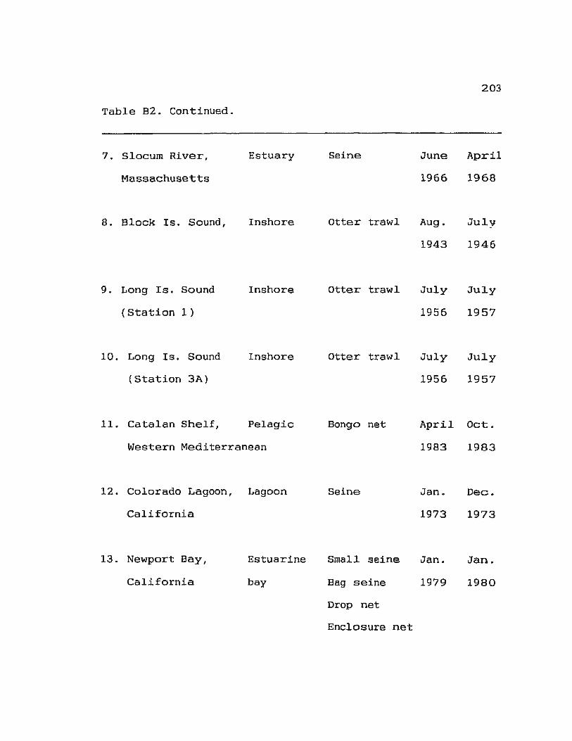
Table 82. Continued.

7. Slocum River,

Massachusetts

8. Block Is. Sound,

9. Long Is. Sound

(Station 1)

10. Long Is. Sound

(Station 3A)

11. Catalan Shelf,

Estuary

Inshore

Inshore

Inshore

Pelagic

Western Mediterranean

12. Colorado Lagoon, Lagoon

California

13. Newport Bay,

California

Estuarine

bay

Seine

Otter trawl

Otter trawl

Otter trawl

Bongo net

Seine

Small seine

Bag seine

Drop net

Enclosure net

June

1966

Aug.

1943

July

1956

July

1956

203

April

1968

July

1946

July

1957

July

1957

April Oct.

1983 1983

Jan.

1973

Jan.

1979

Dec.

1973

Jan.

1980

Table 82. Continued.

14. North Inlet,

South Carolina

Estuary

15. Sapelu 10. St. Cath. Estuary

Sounds, Georgia

16. Apalachee Bay, Salt marsh

N. Florida (Site 4A)

Poison

Otter trawl

Seine

Poison

17. Mustang Island, Surf-zone Seine

Texas

18. Pagbilao Bay, River Otter trawl

Quezon, Philippines

19 . Leaner Swamp , Tidal

Darwin, Australia swamp

Fyke net

Poison

June

1971

Jan.

1967

Aprjl

1971

204

May

1972

Feb.

1968

Sept.

1972

May .1u Ly

1960 1961

March Aug.

1973 19'/4

Oct. Mnrch

1979 1980

20. King's Beach, Surf-zone Coarse seine Sept. Oct.

S. Africa (Coarse net)

21. King ' s Beach, Surf-zone

S. Africa (Fine net)

Fine sei ne

1978 1980

Oct.

1979

Oct.

1980

Table B2. Continued.

22. Cape Coast,

S. Africa

Surf-zone Seine May

1980

205

May

1981