Center for Turbulence ResearchAnnual Research Briefs 2012

127

A matching pursuit approach to solenoidalfiltering of three-dimensional velocity

measurements

By D. Schiavazzi, F. Coletti, G. Iaccarino AND J. K. Eaton

1. Motivation and objectives

Various measurement techniques have been developed recently which provide three-dimensional velocity fields. These methodologies have tremendous potential to improvethe understanding of complex flows in both engineering and biomedical applications.Many flows of interest are effectively incompressible which translates into a zero-divergenceconstraint in the Navier-Stokes equations. Noise and intrinsic errors inevitably affectthree-dimensional flow measurements generating a spurious, finite divergence. The de-velopment of a filter to extract a divergence-free field of minimum distance (in the senseof the closest approximation) from the measurements is therefore of primary interest.Beside improving accuracy, the resulting divergence-free velocity fields are most suitableto extract physical information, notably the pressure field, by integration of the NavierStokes equations.

We propose an iterative procedure which progressively evaluates the `2-nearest zerodivergence field from the available data and is compatible with the measurement resolu-tion. Principles developed in the signal processing community (i.e., Mallat & Zhang 1993)are employed to decompose a velocity field as a linear combination of local solenoidalwaveforms. We also show that the proposed algorithm is naturally parallelizable andtherefore can greatly benefit from implementation on modern GPU architectures.

1.1. OutlineSection 2 describes recent trends in the acquisition of experimental three-dimensionalflow fields, specifically by Particle Image velocimetry (PIV) and Magnetic ResonanceImaging (MRI). The divergence-free condition is reviewed in both local and integralforms in Section 3. The problem of extracting a divergence-free field from measuredvelocities is analyzed in Section 4, where a Sequential Matching Pursuit algorithm isproposed and its convergence is discussed. The proposed algorithm is applied to two-and three-dimensional problems in Sections 5 and 6 in the context of engineering flows.

2. Three-dimensional measurements in fluid mechanics

Real engineering and biomedical flows are complex, three-dimensional phenomena.While numerical simulations naturally provide all three spatial components of the velocityfields for an increasingly large array of problems, results may suffer from oversimplifiedmodeling assumptions or excessive computational cost. On the other hand, experimentaltechniques are typically affected by noise and are available over a limited subset of theentire flow domain. For example, Particle Image Velocimetry (PIV, see Adrian 1991)is a standard technique to evaluate in-plane velocity components over two-dimensional

128 D. Schiavazzi et al.

sections of the flow, whereas Laser-Doppler Velocimetry (LDV) can provide up to threecomponents but at a single location in space. However, recent technological achievementshave led to several approaches capable of measuring the three velocity components over athree-dimensional volume (sometimes referred to as 3D-3C velocity measurements). Thisopens exciting new possibilities for a deeper understanding of complex flow phenomenaas well as new paradigms for extracting information from experiments.

Among the various three-dimensional velocimetry techniques available today, ParticleTracking Velocimetry (PTV) was probably the first to be successfully demonstrated,and it has been employed extensively for the study of Lagrangian particle motion inturbulence (Virant & Dracos 1999). Defocusing digital particle image velocimetry hasbeen applied to single-phase and bubbly flow (Pereira et al. 2000). Scanning-light-sheetPIV has been able to describe complex flow patterns in relatively low flow regimes (Hori& Sakakibara 2004). Holography is three-dimensional in nature and can be very effectivein small measurement volumes (Hinsch & Herrmann 2004). Tomographic PIV (Elsingaet al. 2006) has found the largest success due to its broad applicability and has generatedwidespread interest in the fluid mechanics community.

All the methods listed above are laser-based and require both optical access and seedingof the flow. Therefore they are not suited for biomedical in vivo studies, flow-throughporous media, opaque fluids, or geometrically complex configurations. Approaches basedon medical imaging can eliminate these limitations. Notably, MRI can provide time-averaged three-dimensional velocity fields (Elkins et al. 2003), and it has been extensivelyapplied to industrial and biological problems over the past decade (Elkins & Alley 2007).

3. Local and integral divergence free constraints

The continuity equation in its general expression valid for all flow regimes reads

∂ρ

∂t+∇ · (ρv) = 0, (3.1)

where ρ is the density of the fluid and v is the velocity vector. For a single-componentfluid and low Mach number, (Eq. 3.1) can be written as

∇ · v = 0. (3.2)

Discretization is usually associated with numerical simulations, where weak forms ofPDEs are satisfied in an integral sense on a partition of the computational domain.Assume Ω ⊂ R3 which is compact and has a piecewise smooth boundary ∂Ω. If v is acontinuous and differentiable vector field defined on a neighborhood of Ω of normal n,then we have ∫

Ω

(∇ · v) dΩ =∫

∂Ω

(v · n) dS. (3.3)

In other words, for every simply connected partition of the domain of interest, thedivergence-free condition corresponds to zero net flux across its boundaries. We use theterm locally conservative to identify velocity fields with the above integral property.

4. A signal processing perspective on divergence free filtering

Assume we acquire a finite dimensional representation of a signal f at a discrete numberof locations x(i), i = 1, . . . , N , where N is the total number of available samples. A

Solenoidal MP filtering of 3D velocity measurements 129

representation of f is sought in terms of a set of waveforms (also referred to as atoms),as follows:

f(x(i)) =P∑

j=1

αj wj(x(i)) i = 1, . . . , N or, in matrix form f = Wα, (4.1)

where vector f ∈ RN contains the measurements of signal f , W ∈ RN×P is the waveformdictionary of cardinality P , where columns are discrete realizations of single waveformsand α ∈ RP is the unknown coefficient vector.

The vector α can be computed using different techniques, depending on the choice ofN , P and using prior information on the nature of the resulting approximation. For thecase where N P , an approximate solution α∗ can be computed using a least-squaresminimization of the residual,

α∗ = minα‖f −Wα‖2. (4.2)

This will generate a projection in the space spanned by the atoms in W of minimaldistance (in `2 sense) from the original signal, by solving a symmetric algebraic linearsystem of order N . The solution of a non-symmetric system of equations will lead to asolution of the problem for the case where N = P , for a non-singular and possibly wellconditioned dictionary W. As discussed in the following sections, we are particularlyinterested in the case N < P where the above approximation is sought according to aredundant dictionary of waveforms.

For cases where α is expected to be sparse, greedy approaches or quasi-norm relax-ations within the Compressed Sensing paradigm proved to be efficient in computingaccurate approximations of f (see, e.g., Donoho 2006). In the present case, however, thegoal is to expand the measured velocity field in terms of divergence-free atoms, and theresulting representation is not necessarily sparse. We therefore propose an algorithm tosolve the under-determined system (Eq. 4.1), inspired by the one proposed by Mallat &Zhang (1993).

4.1. Sequential matching pursuit algorithmThe vector f is projected onto spanwi, i = 1, . . . , P by iterative refinements of thecoefficients αi. These coefficients are computed by correlating the i-th waveform with theresidual, as follows:

αi = rTi−1 wi, where ri = ri−1 − αi wi and r0 = f . (4.3)

Note that we always assume a normalized waveform, i.e., ‖wi‖2 = 1, i = 1, . . . , P in ourdevelopment. The reconstructed solution f∗i at the i-th iteration will be computed as

f∗i = f∗i−1 + αi wi, where f∗0 = 0. (4.4)

At every iteration we store the two terms of the decomposition f∗i + ri = f , i.e., thereconstructed solution and the residual vector.

At iteration i the residual ri is orthogonal to atom wi:

wTi ri = wT

i (ri−1 − αi wi) = αi − αi = 0. (4.5)

Therefore, the residual is iteratively orthogonal to the last selected atom, but may not beorthogonal to all others. In general, if the original signal f lies in spanwi, i = 1, . . . , P,then more than P iterations will be required to shrink its norm to zero. In practice, the

130 D. Schiavazzi et al.

algorithm is restarted from the first waveform until the residual becomes smaller than apre-defined threshold.

We now address the convergence of the above methodology, i.e., whether and underwhat circumstances the `2 norm of the residual vector is progressively reduced by iterativeprocedure. We notice that

‖ri‖22 = ‖ri−1 − αi wi‖22 = ‖ri−1‖22 − 2 αi rTi−1 wi + α2

i = ‖ri−1‖22 − α2i , (4.6)

andα2

i =(rT

i−1 wi

)2= ‖ri−1‖22 ‖wi‖22 cos2θ = ‖ri−1‖22 cos2θ. (4.7)

By substitution in Eq. 4.6, we obtain

‖ri‖22 = ‖ri−1‖22(1− cos2θ

)and, by induction ‖ri‖2 = ‖f‖2

i∏n=1

(1− cos2θn

)1/2. (4.8)

Note that the residual is monotonically decreasing and that the rate of convergence atevery iteration depends on the angle θi between the residual at the current iteration andthe selected waveform.

Other methodologies are available in the context of signal processing or CompressedSensing, where the residual is made orthogonal progressively to all the previously se-lected waveforms. For example, the Orthogonal Matching Pursuit (OMP) accomplishesthis task by solving a least-squares minimization problem at every iteration (see, e.g.,Tropp & Gilbert 2007). However, the faster convergence is balanced by increasing thecomputational cost per iteration. Three-dimensional velocity measurements may includeup to a few million cells, and the order of the least-squares problem becomes large withthe iterations. Moreover, for waveforms which are sparse in RN or associated with a pre-defined structure, the correlation and residual update operations can be implementedefficiently even for large datasets.

4.2. Solenoidal atoms for discretized domainsTo describe how local waveforms are computed, we first clarify the quantities of interestfor our idealized vector spaces, e.g., the physical meaning of every single component fi,i = 1, . . . , N of our initial signal. Normal face (edge in 2D) fluxes are used in our approachto encode velocity fields. In practice, we choose N as the total number of faces of ourdiscretization, while fi contains the normal fluxes across face i. The initial vector f canbe assembled in various ways depending on the characteristics of the flow, resolution ofthe available data and boundary conditions.

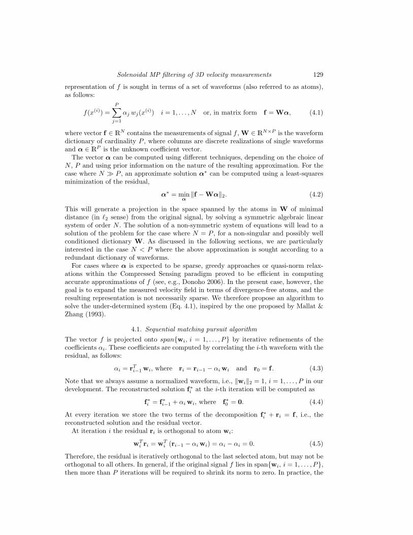
Selection of the best set of atoms for divergence-free projection is driven by variousrequirements. First, the atoms should be compatible with the resolution of the acquireddata. Second, they should be generators for the space of discrete divergence-free flowson the selected partition. In other words, all discrete divergence-free flow patterns in ourmesh should be in spanwi, i = 1, . . . , P. Note that the selected encoding strategy isnaturally suited to represent discrete divergence-free atoms. Examples of atoms are rep-resented in Figure 1, for 2D unstructured and 3D structured discretizations, respectively.

A divergence-free pattern centered at every node is used for 2D applications, whereasedge vortices rotating around global X,Y,Z axes are used in 3D. The fact that the incom-pressible Navier-Stokes equations can be re-written as unsteady transport of vorticitysuggests that a discretized version of the latter could be well employed as a generatorfor any divergence-free flow. Moreover, the above concept can be easily generalized toarbitrary meshes using discrete vortexes defined around every edge in the discretization.

Solenoidal MP filtering of 3D velocity measurements 131

(a) (b) (c) (d)

Figure 1: Examples of divergence-free flux patterns (atoms) for unstructured 2D dis-cretization (a) and structured 3D mesh (b,c,d).

(a) (b) (c)

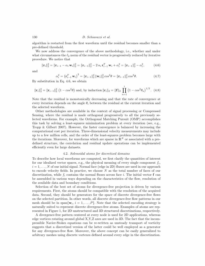
Figure 2: Two-dimensional visualization of faces forming divergence-free atoms (a). Wave-forms with disjoint support whose correlation can be performed concurrently in the firststage (b) and second stage (c) of execution.

To increase the convergence rate of the method, consistent with (Eq. 4.8), every highlycorrelated divergence-free waveform can be added to the dictionary W. For example,a constant flow component, which completely crosses the domain, generally correlatesslowly with local vortex-like diverge-free atoms illustrated in Figure 1. Global atoms aretherefore added in situations consisting of constant fluxes along the three coordinateaxes.

Boundary conditions, with particular reference to a Neumann condition of zero normalflux (solid wall), must be captured in the initial assembling of f and enforced throughoutthe iteration process. A possible strategy is to avoid correlation of the residuals withatoms that are violating the boundary conditions.

The sparsity of a divergence-free atom wi can be understood from its graphical rep-resentation in Figure 1. It is equal to the number of edges shared by a node for the two-dimensional unstructured case, while it always numbers 4 for three-dimensional struc-tured configurations. This means that, in the latter case, only 4 multiplications and 3additions are needed to find the incremental coefficient correlating the components ofthe residual at the current iteration with the non-zero components of wi.

The support of atom wi is defined as the set Γi = j : wi,j 6= 0, i = 1, . . . , P. Wesay the two atoms wi and wj have disjoint support if Γi ∩ Γj = 0. A key featureof the proposed algorithm is that correlation and update with waveforms of disjointsupport can be performed in parallel. For every vortex orientation, practically half ofthe atoms have disjoint support, allowing the above correlations to be performed inonly two stages, assuming a sufficient number of available cores (see Figure 2). In thethree-dimensional structured case, the number of possible concurrent operations when

132 D. Schiavazzi et al.

correlating the residual with one vortex orientation can be estimated as

m =nvortices,X

2=

nc,X(nc,Y + 1)(nc,Z + 1)2

, (4.9)

where nc,X , nc,Y , nc,Z are the number of cells in the X, Y and Z direction, respectively.For example, if nc,X = nc,Y = nc,Z = 10 (1000 cells in total), then m = 605.

Finally, the proposed approach can be used to correlate various encodings (i.e., transla-tion and rotations) of an arbitrary flow pattern, with a given velocity field. For example,a dictionary of waveforms of engineering or clinical interest (vortices, backflows, saddlepoints) could be identified and extracted from the available data.

4.3. Comparison with existing methods

Other techniques to extract the divergence-free components of a measured velocity fieldare described in the literature. A recent publication (Loecher et al. 2012) compares twostrategies developed in the context of clinical applications: the finite difference methodand the radial basis function approach. The first method (Song et al. 2005) uses a 7-pointdiscretization of the Laplacian operator to efficiently solve a Poisson equation using thefast Fourier transform. This technique therefore assumes a structured organization of theacquired field (i.e., measurements on regular grids) and cannot easily be generalized tothe unstructured case. Moreover, the elliptic nature of the Poisson equation raises somequestions on how large local errors in velocity measurements propagate throughout theacquired domain. The second approach (Busch et al. 2012) uses radial basis functionsdefined over a subset of the flow volume. For cases of complex flows, it is not alwaysclear how to define the size of the support for the latter basis and, as a result of adoptingdifferent sizes, the distance of the acquired and filtered velocities may vary.

Our approach differs from the two above. First, divergence-free atoms can also beused for unstructured measurements and Raviart-Thomas interpolation applied to decodevelocities from face fluxes. Moreover, the velocity field is projected on its divergence-freeapproximation of minimal distance. Finally, the selected atoms are the smallest possibledivergence-free waveforms compatible with the measurement grid, and therefore largelocal errors will not be propagated to neighboring velocities.

5. Application to two-dimensional numerical simulation of two-dimensionaldiffusion

The proposed procedure is applied to correct the velocity field computed by solvingthe diffusion equation with a Galerkin residual formulation on linear triangles.

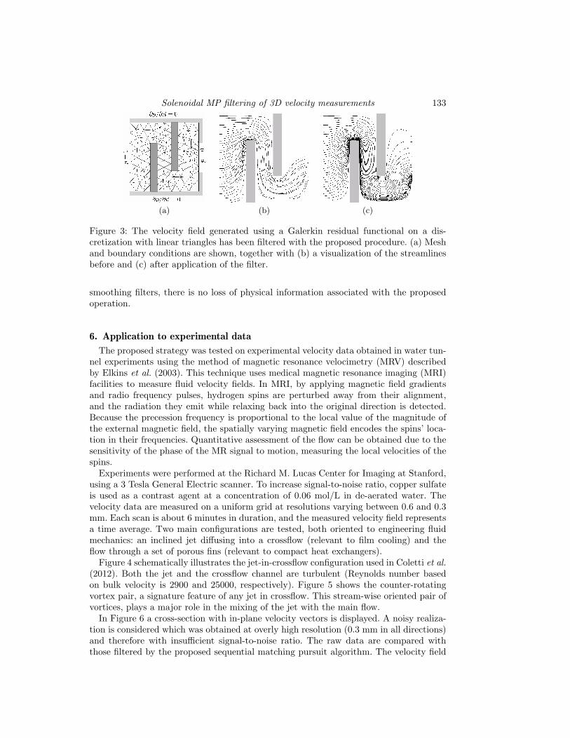
Results are shown in terms of streamlines generated using a Euler approach andelement-wise constant velocities (Figure 3). The streamlines start from the left edgeand, given the imposed pressure difference, should exit from the right edge. Only a fewstreamlines are able to follow the correct velocity path in the Galerkin solution, as thevelocity field is not locally conservative. Application of the proposed divergence-free con-straint significantly improves streamline paths, allowing nearly all of them to reach theexit.

Note that the application of the sequential matching pursuit heuristic is intended asa filter for the measured fields rather than as a correction, meaning that a divergence-free field is extracted from the measurements and that the latter are not corrected byintroducing information not originally contained in the data. However, unlike standard

Solenoidal MP filtering of 3D velocity measurements 133

(a) (b) (c)

Figure 3: The velocity field generated using a Galerkin residual functional on a dis-cretization with linear triangles has been filtered with the proposed procedure. (a) Meshand boundary conditions are shown, together with (b) a visualization of the streamlinesbefore and (c) after application of the filter.

smoothing filters, there is no loss of physical information associated with the proposedoperation.

6. Application to experimental data

The proposed strategy was tested on experimental velocity data obtained in water tun-nel experiments using the method of magnetic resonance velocimetry (MRV) describedby Elkins et al. (2003). This technique uses medical magnetic resonance imaging (MRI)facilities to measure fluid velocity fields. In MRI, by applying magnetic field gradientsand radio frequency pulses, hydrogen spins are perturbed away from their alignment,and the radiation they emit while relaxing back into the original direction is detected.Because the precession frequency is proportional to the local value of the magnitude ofthe external magnetic field, the spatially varying magnetic field encodes the spins’ loca-tion in their frequencies. Quantitative assessment of the flow can be obtained due to thesensitivity of the phase of the MR signal to motion, measuring the local velocities of thespins.

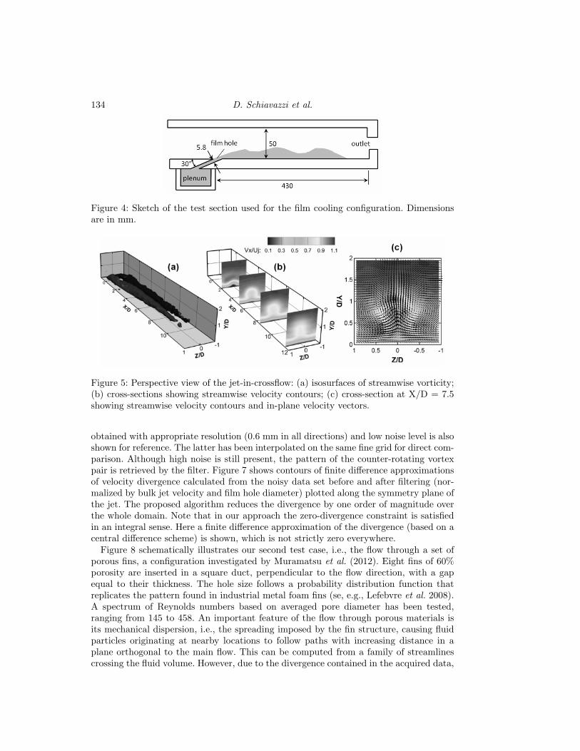
Experiments were performed at the Richard M. Lucas Center for Imaging at Stanford,using a 3 Tesla General Electric scanner. To increase signal-to-noise ratio, copper sulfateis used as a contrast agent at a concentration of 0.06 mol/L in de-aerated water. Thevelocity data are measured on a uniform grid at resolutions varying between 0.6 and 0.3mm. Each scan is about 6 minutes in duration, and the measured velocity field representsa time average. Two main configurations are tested, both oriented to engineering fluidmechanics: an inclined jet diffusing into a crossflow (relevant to film cooling) and theflow through a set of porous fins (relevant to compact heat exchangers).

Figure 4 schematically illustrates the jet-in-crossflow configuration used in Coletti et al.(2012). Both the jet and the crossflow channel are turbulent (Reynolds number basedon bulk velocity is 2900 and 25000, respectively). Figure 5 shows the counter-rotatingvortex pair, a signature feature of any jet in crossflow. This stream-wise oriented pair ofvortices, plays a major role in the mixing of the jet with the main flow.

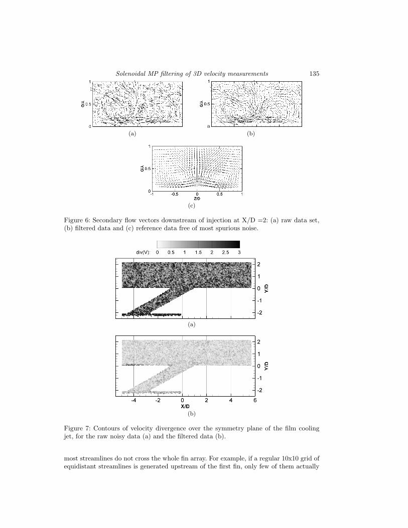
In Figure 6 a cross-section with in-plane velocity vectors is displayed. A noisy realiza-tion is considered which was obtained at overly high resolution (0.3 mm in all directions)and therefore with insufficient signal-to-noise ratio. The raw data are compared withthose filtered by the proposed sequential matching pursuit algorithm. The velocity field

134 D. Schiavazzi et al.

Figure 4: Sketch of the test section used for the film cooling configuration. Dimensionsare in mm.

Figure 5: Perspective view of the jet-in-crossflow: (a) isosurfaces of streamwise vorticity;(b) cross-sections showing streamwise velocity contours; (c) cross-section at X/D = 7.5showing streamwise velocity contours and in-plane velocity vectors.

obtained with appropriate resolution (0.6 mm in all directions) and low noise level is alsoshown for reference. The latter has been interpolated on the same fine grid for direct com-parison. Although high noise is still present, the pattern of the counter-rotating vortexpair is retrieved by the filter. Figure 7 shows contours of finite difference approximationsof velocity divergence calculated from the noisy data set before and after filtering (nor-malized by bulk jet velocity and film hole diameter) plotted along the symmetry plane ofthe jet. The proposed algorithm reduces the divergence by one order of magnitude overthe whole domain. Note that in our approach the zero-divergence constraint is satisfiedin an integral sense. Here a finite difference approximation of the divergence (based on acentral difference scheme) is shown, which is not strictly zero everywhere.

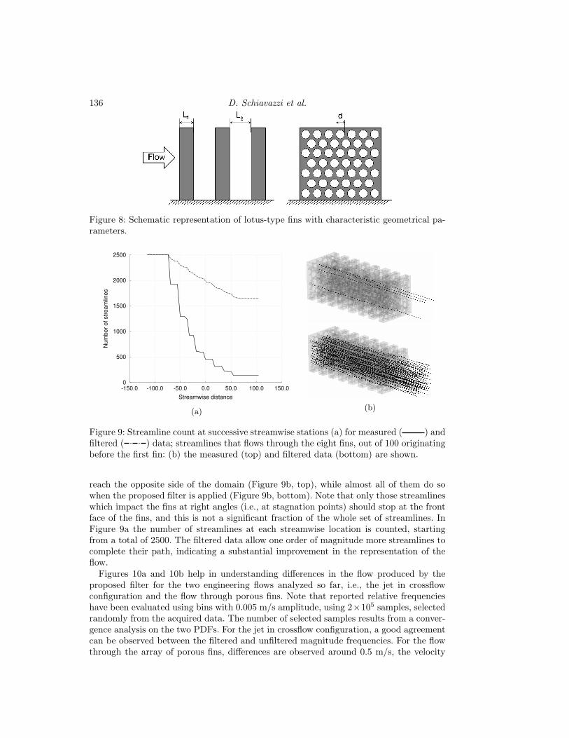
Figure 8 schematically illustrates our second test case, i.e., the flow through a set ofporous fins, a configuration investigated by Muramatsu et al. (2012). Eight fins of 60%porosity are inserted in a square duct, perpendicular to the flow direction, with a gapequal to their thickness. The hole size follows a probability distribution function thatreplicates the pattern found in industrial metal foam fins (se, e.g., Lefebvre et al. 2008).A spectrum of Reynolds numbers based on averaged pore diameter has been tested,ranging from 145 to 458. An important feature of the flow through porous materials isits mechanical dispersion, i.e., the spreading imposed by the fin structure, causing fluidparticles originating at nearby locations to follow paths with increasing distance in aplane orthogonal to the main flow. This can be computed from a family of streamlinescrossing the fluid volume. However, due to the divergence contained in the acquired data,

Solenoidal MP filtering of 3D velocity measurements 135

(a) (b)

(c)

Figure 6: Secondary flow vectors downstream of injection at X/D =2: (a) raw data set,(b) filtered data and (c) reference data free of most spurious noise.

(a)

(b)

Figure 7: Contours of velocity divergence over the symmetry plane of the film coolingjet, for the raw noisy data (a) and the filtered data (b).

most streamlines do not cross the whole fin array. For example, if a regular 10x10 grid ofequidistant streamlines is generated upstream of the first fin, only few of them actually

136 D. Schiavazzi et al.

Figure 8: Schematic representation of lotus-type fins with characteristic geometrical pa-rameters.

0

500

1000

1500

2000

2500

-150.0 -100.0 -50.0 0.0 50.0 100.0 150.0

Nu

mb

er

of

str

ea

mlin

es

Streamwise distance

(a) (b)

Figure 9: Streamline count at successive streamwise stations (a) for measured ( ) andfiltered ( ) data; streamlines that flows through the eight fins, out of 100 originatingbefore the first fin: (b) the measured (top) and filtered data (bottom) are shown.

reach the opposite side of the domain (Figure 9b, top), while almost all of them do sowhen the proposed filter is applied (Figure 9b, bottom). Note that only those streamlineswhich impact the fins at right angles (i.e., at stagnation points) should stop at the frontface of the fins, and this is not a significant fraction of the whole set of streamlines. InFigure 9a the number of streamlines at each streamwise location is counted, startingfrom a total of 2500. The filtered data allow one order of magnitude more streamlines tocomplete their path, indicating a substantial improvement in the representation of theflow.

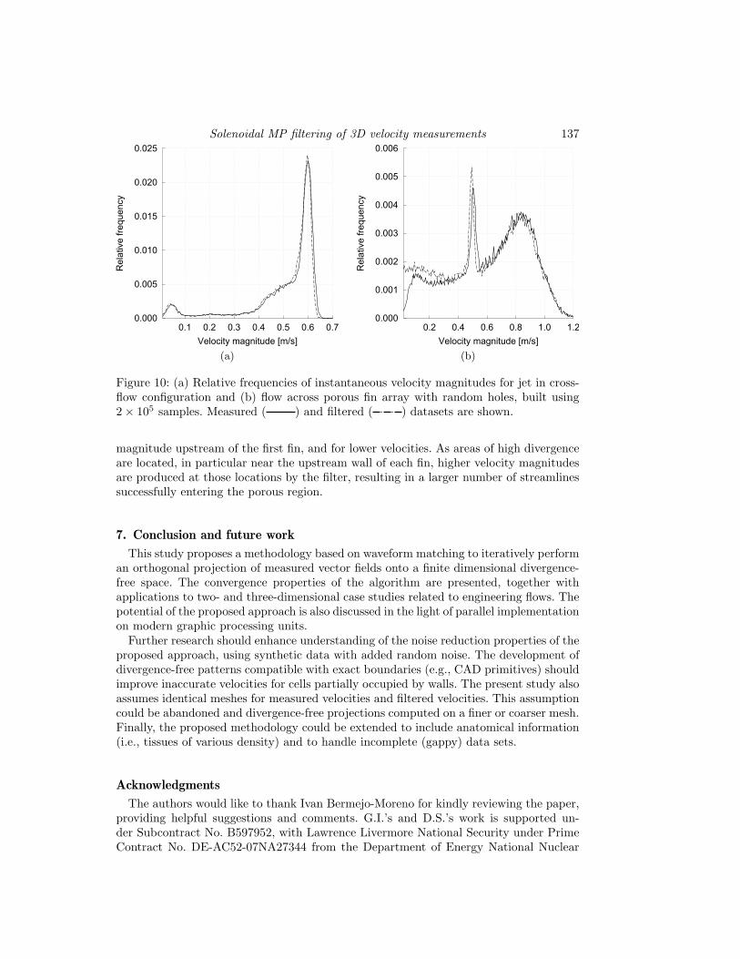
Figures 10a and 10b help in understanding differences in the flow produced by theproposed filter for the two engineering flows analyzed so far, i.e., the jet in crossflowconfiguration and the flow through porous fins. Note that reported relative frequencieshave been evaluated using bins with 0.005 m/s amplitude, using 2×105 samples, selectedrandomly from the acquired data. The number of selected samples results from a conver-gence analysis on the two PDFs. For the jet in crossflow configuration, a good agreementcan be observed between the filtered and unfiltered magnitude frequencies. For the flowthrough the array of porous fins, differences are observed around 0.5 m/s, the velocity

Solenoidal MP filtering of 3D velocity measurements 137

0.000

0.005

0.010

0.015

0.020

0.025

0.1 0.2 0.3 0.4 0.5 0.6 0.7

Rel

ativ

esfr

eque

ncy

Velocitysmagnitudes[m/s]

(a)

0.000

0.001

0.002

0.003

0.004

0.005

0.006

0.2 0.4 0.6 0.8 1.0 1.2

Rel

ativ

esfr

eque

ncy

Velocitysmagnitudes[m/s]

(b)

Figure 10: (a) Relative frequencies of instantaneous velocity magnitudes for jet in cross-flow configuration and (b) flow across porous fin array with random holes, built using2× 105 samples. Measured ( ) and filtered ( ) datasets are shown.

magnitude upstream of the first fin, and for lower velocities. As areas of high divergenceare located, in particular near the upstream wall of each fin, higher velocity magnitudesare produced at those locations by the filter, resulting in a larger number of streamlinessuccessfully entering the porous region.

7. Conclusion and future work

This study proposes a methodology based on waveform matching to iteratively performan orthogonal projection of measured vector fields onto a finite dimensional divergence-free space. The convergence properties of the algorithm are presented, together withapplications to two- and three-dimensional case studies related to engineering flows. Thepotential of the proposed approach is also discussed in the light of parallel implementationon modern graphic processing units.

Further research should enhance understanding of the noise reduction properties of theproposed approach, using synthetic data with added random noise. The development ofdivergence-free patterns compatible with exact boundaries (e.g., CAD primitives) shouldimprove inaccurate velocities for cells partially occupied by walls. The present study alsoassumes identical meshes for measured velocities and filtered velocities. This assumptioncould be abandoned and divergence-free projections computed on a finer or coarser mesh.Finally, the proposed methodology could be extended to include anatomical information(i.e., tissues of various density) and to handle incomplete (gappy) data sets.

Acknowledgments

The authors would like to thank Ivan Bermejo-Moreno for kindly reviewing the paper,providing helpful suggestions and comments. G.I.’s and D.S.’s work is supported un-der Subcontract No. B597952, with Lawrence Livermore National Security under PrimeContract No. DE-AC52-07NA27344 from the Department of Energy National Nuclear

138 D. Schiavazzi et al.

Security Administration for the management and operation of the Lawrence LivermoreNational Laboratory. F.C.’s work is supported by a grant from the Honeywell Corpora-tion.

REFERENCES

Adrian, R. 1991 Particle-imaging techniques for experimental fluid mechanics. Ann.Rev. of Fluid Mechanics 23, 261–304.

Busch, J., Giese, D., Wissmann, L. & Kozerke, S. 2012 Construction of divergence-free velocity fields from cine 3D phase-contrast flow measurements. Journal of Car-diovascular Magnetic Resonance 14, W38.

Coletti, F., Elkins, C. & Eaton, J. 2012 An inclined jet in crossflow under theeffect of streamwise pressure gradients. Experiments in Fluids - Submitted.

Donoho, D. 2006 Compressed sensing. Information Theory, IEEE Transactions on 52,1289–1306.

Elkins, C. & Alley, M. 2007 Magnetic Resonance Velocimetry: applications of mag-netic resonance imaging in the measurement of fluid motion. Experiments in Fluids43, 823–858.

Elkins, C., Markl, M., Pelc, N. & Eaton, J. 2003 4D Magnetic resonance ve-locimetry for mean velocity measurements in complex turbulent flows. Experimentsin Fluids 34, 494–503.

Elsinga, G., Scarano, F., Wieneke, B. & Van Oudheusden, B. 2006 Tomographicparticle image velocimetry. Experiments in Fluids 41, 933–947.

Hinsch, K. & Herrmann, S. 2004 Holographic particle image velocimetry. Measure-ment Science and Technology 15.

Hori, T. & Sakakibara, J. 2004 High-speed scanning stereoscopic PIV for 3D vorticitymeasurement in liquids. Measurement Science and Technology 15, 1067.

Lefebvre, L., Banhart, J. & Dunand, D. 2008 Porous metals and metallic foams:current status and recent developments. Advanced Engineering Materials 10, 775–787.

Loecher, M., Kecskemeti, S., Turski, P. & Wieben, O. 2012 Comparison ofdivergence-free algorithms for 3D MRI with three-directional velocity encoding.Journal of Cardiovascular Magnetic Resonance 14, 1–2.

Mallat, S. & Zhang, Z. 1993 Matching pursuits with time-frequency dictionaries.Signal Processing, IEEE Transactions on 41, 3397–3415.

Muramatsu, K., Coletti, F., Elkins, C. & Eaton, J. 2012 Fluid flow and mechan-ical dispersion through porous fins. Physics of Fluids - Submitted.

Pereira, F., Gharib, M., Dabiri, D. & Modarress, D. 2000 Defocusing digitalparticle image velocimetry: a 3-component 3-dimensional DPIV measurement tech-nique. Application to bubbly flows. Experiments in Fluids 29, 78–84.

Song, S., Napel, S., Glover, G. & Pelc, N. 2005 Noise reduction in three-dimensional phase-contrast MR velocity measurements. Journal of Magnetic Res-onance Imaging 3, 587–596.

Tropp, J. & Gilbert, A. 2007 Signal recovery from random measurements via orthog-onal matching pursuit. Information Theory, IEEE Transactions on 53, 4655–4666.

Virant, M. & Dracos, T. 1999 3D PTV and its application on lagrangian motion.Measurement Science and Technology 8, 1539.