Center for Turbulence Research Annual Research Briefs 2009

Center for Turbulence ResearchAnnual Research Briefs 2009

145

Role of Weber number in primary breakup ofturbulent liquid jets in crossflow

By M. G. Pai, I. Bermejo-Moreno, O. Desjardins† AND H. Pitsch

1. Motivation and objectives

Atomization of liquid fuel controls combustion efficiency and pollutant emissions ofinternal combustion engines and gas turbines (Lefebvre 1998). The liquid jet in crossflow(LJCF) finds application in lean premixed prevaporized (LPP) ducts, afterburners forgas turbines, and combustors for ramjets and scramjets. This flow configuration, whichconsists of a turbulent liquid jet injected transversely into a gaseous laminar or turbulentcrossflow, has been the focus of several experimental studies with the primary objectiveof proposing scaling laws and regime diagrams for liquid breakup (Sallam et al. 2004; Leeet al. 2007; Bellofiore, A. 2006). A typical turbulent LJCF exhibits a Kelvin-Helmoholtz-type instability wave on the windward side of the liquid column (see schematic in Fig. 1).These waves travel along the liquid column and ultimately lead to its breakup aroundthe time the liquid jet reaches the maximum penetration in the transverse direction. Forhigh crossflow Weber number and momentum flux ratios, a turbulent liquid jet with acircular cross-section gradually changes into an almost crescent shape. Ligaments, drops,and other liquid structures, which are termed dispersed phase elements (DPEs) in therest of this brief, are shed along the sides of the liquid column especially along the crescentedges. The shedding of DPEs is more prominent at the location of the traveling wavesand might be a primary source of DPE production in the LJCF. Primary breakup inthe context of a LJCF refers to this first stage of liquid jet breakup, which involves theshedding of DPEs from the liquid column owing to various processes inside the liquidjet and the ambient gas. In the primary breakup stage, DPEs that are shed from theliquid column need not be spherical in shape (see Fig. 1). Depending on the size andvelocity of the DPEs (as characterized, say, by the Weber number and Reynolds numbercorresponding to these structures) that are shed from the liquid column as a result ofprimary breakup, these DPEs undergo further breakup. This second stage of breakupis termed secondary breakup. Experiments report the drop size distribution that resultsafter primary and secondary breakup, in addition to coalescence of drops and ligamentsfurther downstream, and possibly other sources of drop formation (for instance, satellitedrop formation as a result of rebounding drops). Thus a primary breakup model forthe LJCF must be able to capture the size distribution (or more precisely, the volumedistribution) and possibly other geometrical features of the DPEs immediately after beingshed from the liquid column in order to be predictive. This information would be suppliedto a secondary breakup model, which then predicts a drop size distribution that can beemployed in numerical calculations of multiphase reactive flows with sprays.

Several experiments have shed light on various regimes of breakup and scaling lawsfor various statistics such as liquid jet penetration and trajectory, Sauter mean diam-eter of drops and wavelength of liquid surface instabilities have been proposed. Yet,

† Department of Mechanical Engineering, University of Colorado, Boulder, Colorado, USA.

146 M. G. Pai et al.

Figure 1. Schematic of a turbulent liquid jet in crossflow illustrating a typical breakup scenario.Large liquid structures, ligaments and drops that have just broken off the liquid column andclassified to be part of the primary breakup regime are shown in dark grey. Ligaments and dropsshown in light grey constitute the secondary breakup regime.

predictive models for primary breakup of turbulent LJCF are still unavailable. Usingexperiments, it is challenging to perform detailed parametric studies of a LJCF by vary-ing one dimensionless group while fixing the remaining dimensionless groups. However,simple changes of parameters do not pose a challenge to numerical studies. In a recentnumerical study (Pai et al. 2008, 2009), we demonstrated that the liquid Weber number,rather than the crossflow Weber number, controls the wavelength of liquid surface insta-bilities on the windward side of the LJCF. This was seemingly in contradiction with ascaling that was proposed using experimental datasets (Sallam et al. 2004). On carefulinterpretation of the experimental dataset however, this seeming contradiction was re-solved (see Pai et al. 2009 for details) and, interestingly, the experimental observationswere in accord with the numerical results. That study underscored the importance ofcarefully interpreting scaling laws obtained from experiments before using such scalinglaws to build primary breakup models.

In the earlier numerical study (Pai et al. 2009), the focus was on liquid structurescorresponding to the LJCF whose size was on the order of the injector diameter. Theassumption was that such structures would be resolved well by the grid and that ne-glecting the smaller unresolved liquid and gas-phase structures would not affect the largescale structures. In this study, we perform a subset of the simulations from the previousparametric study at the mesh resolution that is necessary to resolve the smallest lengthscales in the problem. In addition, we investigate the geometrical characteristics of theDPEs that separate from the liquid column using concepts from differential geometry,details of which are provided below.

We begin by reviewing the governing equations for the primary breakup of liquid jets.The scope of the current study is reviewed followed by a discussion on some of thecomputational details. A discussion of results obtained from the parametric study andthe geometrical analysis is presented next. The study concludes with a summary of theprincipal results and an outlook for future studies.

Role of Weber number in primary breakup 147

2. Governing equations

We assume constant thermodynamic properties of the liquid and gas phases and use theincompressible Navier-Stokes (NS) equations to describe the problem of liquid breakup:

∂u

∂t+ u · ∇u = −1

ρ∇p +

1

ρ∇ ·

(

µ(

∇u + (∇u)T))

, (2.1)

where u is the velocity, p is the pressure, ρ is the thermodynamic density, and µ is thedynamic viscosity. The continuity equation

∂ρ

∂t+ ∇ · ρu = 0 (2.2)

and the incompressibility constraint Dρ/Dt = 0 imply that the velocity field is solenoidal.If Γ represents the interface that separates the two immiscible fluids or phases, then thefollowing condition holds at the interface:

[p]Γ = σκ +

[

µ

(

∂ui

∂xj+

∂uj

∂xi

)

ninj

]

Γ

(2.3)

where [Q]Γ = Q+ − Q−

represents the jump of a quantity Q, which has values Q+ andQ

−on either side of the interface, κ is the mean curvature, σ is the interfacial tension,

and n is the unit normal to the interface. We denote the (+) side to be in the liquid (liq)and the (−) side to be in the gas (g). The jump condition in Eq. (2.3) can be simplifiedto (Kang et al. 2000)

[p]Γ = σκ + 2 [µ]Γ∂ui

∂xjninj, (2.4)

where [µ]Γ is a constant non-zero jump in the viscosity across the interface. Since thetwo fluids have different densities, there is a jump in the density, i.e., [ρ]Γ = constantacross the interface (we assume constant viscosity and density in the two fluids). Fromthe conservation of mass, it follows that for a flow with no interphase mass transfer, thevelocity at the interface is continuous, i.e., [u]Γ = 0.

A simple analysis of the dimensional quantities that characterize the LJCF revealsthat from among the seven non-dimensional groups that characterize the LJCF, whichare crossflow Weber number, liquid Weber number, liquid-gas density ratio, momentumflux ratio, liquid Reynolds number, cross-flow Reynolds number, and Ohnesorge number,only five are independent (see Pai et al. 2009 for more details).

3. Scope of current study

Although the primary purpose of this study is to understand the implications of highermesh resolution on the liquid jet breakup, the present work also investigates the geomet-rical characteristics of the DPEs that result from the shedding of ligaments and drops inthe domain. From the perspective of primary breakup modeling, it is necessary to quan-tify the geometrical characteristics of DPEs immediately after being shed from the liquidcolumn. However, in this preliminary study, we focus on the geometrical characteristicsof the DPEs in the entire computational domain at a certain characteristic timescale.

From among the five non-dimensional groups that characterize the LJCF, we investi-gate the role of liquid Weber number and crossflow Weber number in the primary breakupof a liquid jet in crossflow. The liquid Weber number characterizes the tendency of theliquid jet to break up owing to a competition between liquid inertia and surface tension


forces, whereas the crossflow Weber number characterizes the tendency of the liquid jetto break up owing to a competition between the gas-phase inertia and surface tensionforces.

4. Computational details

4.1. Numerical methology

In this study, a spectrally refined interface tracking scheme for the level set functionis employed (Desjardins & Pitsch 2009). This interface tracking technique has severaladvantages over other available methods such as the volume of fluid (VOF) (Scardovelli& Zaleski 1999), coupled level set/volume of fluid (CLSVOF) (Sussman et al. 2007),and Lagrangian particle-based methods (Hieber & Koumoutsakos 2005). See Desjardins(2008) for a detailed discussion. In SRI, the level set field is represented on a finite numberof subcell quadrature nodes around the interface. The level set field is advected using asemi-Lagrangian approach, which takes advantage of the fact that the level set equationgiven by

∂G

∂t+ u · ∇G =

DG

Dt= 0, (4.1)

where G(x, t) is the level set field, is a constant along the trajectory of material pointsmoving at velocity u. At the new location x

n+1 and time tn+1, the value of the level setfunction corresponding to each quadrature node is computed by integrating backward intime to the previous position x

n at tn along the material point trajectory that passesthrough x

n+1. The value of Gn+1(xn+1) is then set equal to Gn at location xn. As high-

order schemes can be used to numerically integrate along the material point trajectory,numerical diffusion of the interface is minimal. This method, in conjunction with thesubcell resolution, allows for retaining sharp features of the interface as the liquid jetevolves in time (see Desjardins & Pitsch 2009; Pai et al. 2009 for details).

A high-order conservative finite difference scheme (Desjardins et al. 2008a) is built intoan in-house code called NGA, which has been efficiently written with MPI libraries forlarge-scale distributed memory computations. The variables are staggered in space andtime, and centered finite difference schemes are employed. Accurate jump conditions forthe pressure given by Eq. (2.4) that include the surface tension force are imposed usinga ghost fluid (GF) method (Desjardins et al. 2008b). Only second-order accuracy will beemployed here as the formal order of accuracy is limited by the interfacial GF treatment,which is currently first-order. In order to allow for an implicit treatment of the viscousterms in the NS equations in conjuction with an approximate factorization technique,we adopt a continuous surface force (CSF) formulation for the viscosity. This essentiallyremoves the jump in viscosity in Eq. (2.4) and thus the pressure jump contains only thesurface tension.

4.2. Computational expense

Resolution requirements for the LJCF are dictated by the need to resolve the smallestlength scales in the gas phase and liquid phase, which are primarily governed by theReynolds number corresponding to each phase, and the smallest structures formed duringliquid breakup, which are primarily governed by the liquid and crossflow Weber number.

We use a turbulent pipe flow for the liquid injection, so the smallest length scales inthe liquid jet are governed by the liquid Reynolds number based on injector diameterd, Reliq = ρlUliqd/µliq. Assuming a uniform mesh resolution ∆x = 2δv, where δv is the


viscous length scale in the turbulent pipe flow, we obtain a scaling for the number ofpoints along the injector diameter Ndia = d/∆x with Reliq as (see Pai et al. 2009 fordetails)

Ndia = 0.1 Re7/8

liq . (4.2)

For droplet-laden flows, the liquid Weber number decides the competitive effects of inertiaand surface tension forces and thus the likelihood of a drop to undergo further breakup.Theoretical analyses (Hinze 1955) and experiments (Lefebvre 1998) suggest that dropswith liquid Weber number less than ∼ 10 normally do not undergo further breakup. Theneed to resolve droplets (or liquid structures) until this limit imposes a requirement on thesmallest grid size in the computational domain. In other words, we require that the Webernumber based on the grid size ∆x, We∆x, be less than 10, i.e., We∆x = ρlU

2l ∆x/σ < 10

from which a criterion on Ndia arises as

Ndia > 0.1Weliq. (4.3)

For the cases considered here, the crossflow Weber number (Wecf) based on the injectordiameter is less than the liquid Weber number (Weliq), so the above requirement for Ndia

based on Weliq is more restrictive.

From the foregoing analysis, an estimate for the grid size required in the entire com-putational domain is

NtotE = (Cxb + nxb)(Cyb + nyb)nzq1/2 max ( 0.001We3

liq/r3, 0.001Re21/8

liq ), (4.4)

where nxb = 3 and nyb = 4 account for an additional buffer region upstream of theinjector inlet for the flow to develop around the liquid column, and along the y direction,respectively. Also, r + 1 is the number of quadrature nodes in each cell (see discussionbelow). Note that since this estimate is obtained by using a uniform grid everywhere inthe computational domain, it can be considered as an upper bound on the grid size.

Liquid structures smaller than the flow solver (velocity-pressure) cell can potentiallybe retained as the SRI method provides subcell resolution Desjardins & Pitsch (2009).One may resolve up to r times larger Weber numbers by adopting the subcell resolutioncompared to that resolved on the flow solver grid. Although this is the case, we use r = 2in the current study. This essentially implies that a flow solver cell has 27 quadraturenodes with one of these nodes at the cell center. The primary reason for employing r = 2rather than r = 4 as in Pai et al. (2009) is the significant computational expense in termsof memory that one incurs with increasing r, especially when the flow solver resolutionis itself very high (see Table 1). For instance, r = 2 implies 27 additional memorylocations, whereas r = 4 implies 125 additional memory locations to retain informationon the sub-cell G field in each flow solver cell. For instance, if there are 200,000 flowsolver cells on each process in a parallel computing environment, and assuming that 25%of these cells have subcell resolution due to the presence of the interface, the overhead isaround 1 million additional memory locations for r = 2 and 6 million additional memorylocations for r = 4. Especially at high Weber number Weliq > 500, there are regions inthe computational domain where all the 200, 000 flow solver cells have subcell resolution.Load balancing under these circumstances becomes an enormous challenge, especiallyfor the inhomogeneous geometry that is under consideration and the uniform domaindecomposition adopted in this study. Incorporating an efficient, adaptive load balancingtechnique in the context of the SRI methodology is left as a future exercise.


(a) (b)

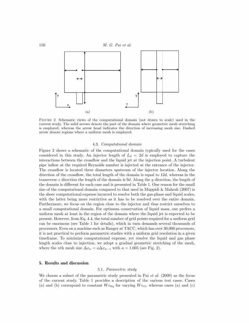
Figure 2. Schematic views of the computational domain (not drawn to scale) used in thecurrent study. The solid arrows denote the part of the domain where geometric mesh stretchingis employed, whereas the arrow head indicates the direction of increasing mesh size. Dashedarrow denote regions where a uniform mesh is employed.

4.3. Computational domain

Figure 2 shows a schematic of the computational domain typically used for the casesconsidered in this study. An injector length of Ld = 2d is employed to capture theinteractions between the crossflow and the liquid jet at the injection point. A turbulentpipe inflow at the required Reynolds number is injected at the entrance of the injector.The crossflow is located three diameters upstream of the injector location. Along thedirection of the crossflow, the total length of the domain is equal to 12d, whereas in thetransverse z direction the length of the domain is 9d. Along the y direction, the length ofthe domain is different for each case and is presented in Table 1. One reason for the smallsize of the computational domain compared to that used in Muppidi & Mahesh (2007) isthe sheer computational expense incurred to resolve both the gas-phase and liquid scales,with the latter being more restrictive as it has to be resolved over the entire domain.Furthermore, we focus on the region close to the injector and thus restrict ourselves toa small computational domain. For optimum conservation of liquid mass, one prefers auniform mesh at least in the region of the domain where the liquid jet is expected to bepresent. However, from Eq. 4.4, the total number of grid points required for a uniform gridcan be enormous (see Table 1 for details), which in turn demands several thousands ofprocessors. Even on a machine such as Ranger at TACC, which has over 30,000 processors,it is not practical to perform parametric studies with a uniform grid resolution in a giventimeframe. To minimize computational expense, yet resolve the liquid and gas phaselength scales close to injection, we adopt a gradual geometric stretching of the mesh,where the nth mesh size ∆xn = a∆xn−1 with a = 1.005 (see Fig. 2).

5. Results and discussion

5.1. Parametric study

We choose a subset of the parametric study presented in Pai et al. (2009) as the focusof the current study. Table 1 provides a description of the various test cases. Cases(a) and (b) correspond to constant Weliq for varying Wecf , whereas cases (a) and (c)


Cases q Wecf Weliq Reliq Ndia Ntot Lx, Ly , Lz Nproc NtotE

(actual) (times d) (Eq. 4.4)

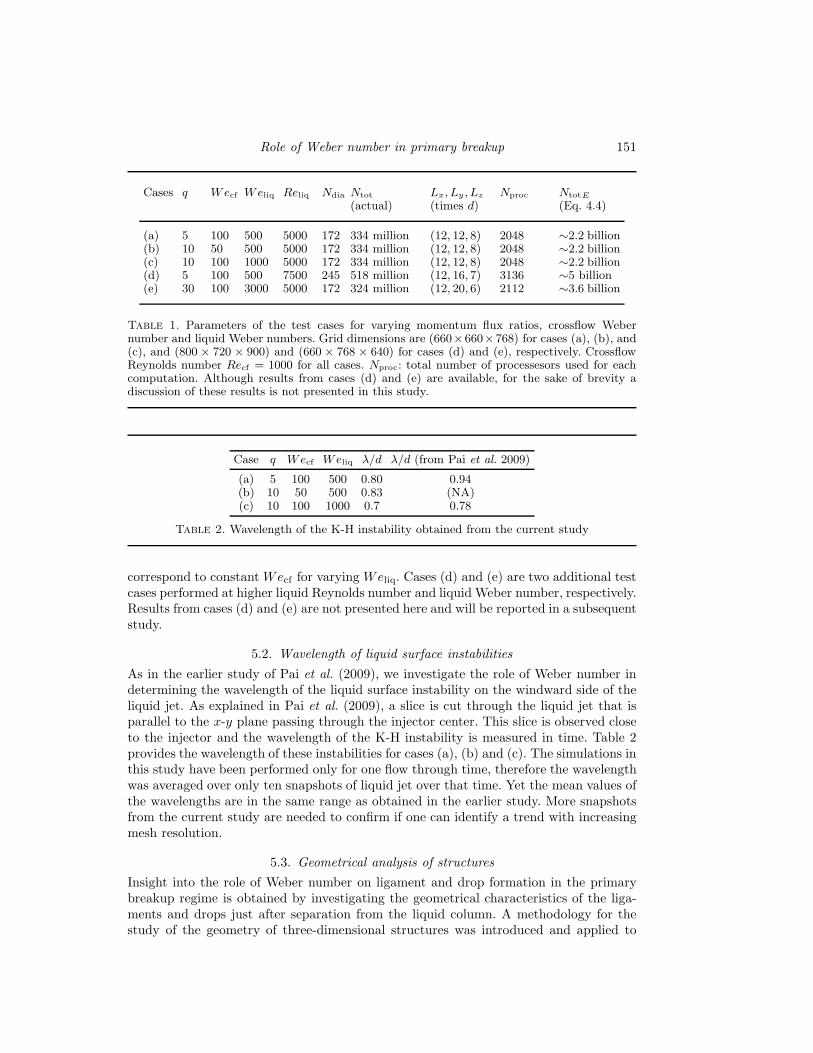
(a) 5 100 500 5000 172 334 million (12, 12, 8) 2048 ∼2.2 billion(b) 10 50 500 5000 172 334 million (12, 12, 8) 2048 ∼2.2 billion(c) 10 100 1000 5000 172 334 million (12, 12, 8) 2048 ∼2.2 billion(d) 5 100 500 7500 245 518 million (12, 16, 7) 3136 ∼5 billion(e) 30 100 3000 5000 172 324 million (12, 20, 6) 2112 ∼3.6 billion

Table 1. Parameters of the test cases for varying momentum flux ratios, crossflow Webernumber and liquid Weber numbers. Grid dimensions are (660×660×768) for cases (a), (b), and(c), and (800 × 720 × 900) and (660 × 768 × 640) for cases (d) and (e), respectively. CrossflowReynolds number Recf = 1000 for all cases. Nproc: total number of processesors used for eachcomputation. Although results from cases (d) and (e) are available, for the sake of brevity adiscussion of these results is not presented in this study.

Case q Wecf Weliq λ/d λ/d (from Pai et al. 2009)

(a) 5 100 500 0.80 0.94(b) 10 50 500 0.83 (NA)(c) 10 100 1000 0.7 0.78

Table 2. Wavelength of the K-H instability obtained from the current study

correspond to constant Wecf for varying Weliq. Cases (d) and (e) are two additional testcases performed at higher liquid Reynolds number and liquid Weber number, respectively.Results from cases (d) and (e) are not presented here and will be reported in a subsequentstudy.

5.2. Wavelength of liquid surface instabilities

As in the earlier study of Pai et al. (2009), we investigate the role of Weber number indetermining the wavelength of the liquid surface instability on the windward side of theliquid jet. As explained in Pai et al. (2009), a slice is cut through the liquid jet that isparallel to the x-y plane passing through the injector center. This slice is observed closeto the injector and the wavelength of the K-H instability is measured in time. Table 2provides the wavelength of these instabilities for cases (a), (b) and (c). The simulations inthis study have been performed only for one flow through time, therefore the wavelengthwas averaged over only ten snapshots of liquid jet over that time. Yet the mean values ofthe wavelengths are in the same range as obtained in the earlier study. More snapshotsfrom the current study are needed to confirm if one can identify a trend with increasingmesh resolution.

5.3. Geometrical analysis of structures

Insight into the role of Weber number on ligament and drop formation in the primarybreakup regime is obtained by investigating the geometrical characteristics of the liga-ments and drops just after separation from the liquid column. A methodology for thestudy of the geometry of three-dimensional structures was introduced and applied to


single-phase turbulent flows in Bermejo-Moreno & Pullin (2008). In the present study,we consider a subset (namely, the geometrical characterization step) of that methodologyto analyze structures educed from instantaneous snapshots of the evolution of turbulentliquid jets in cross flow. Although as noted earlier, the focus of the geometrical character-ization should be the ligaments that have just separated from the liquid column, in thisstudy we focus on all the liquid structures that have separated from the liquid columnuntil a certain characteristic time (see below). In this preliminary study, the effect of thephysical parameters q, Weliq, and Wecf on the liquid structure geometry for two differentinstants in time is reported.

5.3.1. Methodology

At every point of a given closed surface with area A and volume V , we obtain twodifferential geometry properties: the absolute value of the shape index S̃, and the dimen-sionless curvedness C̃ (non-dimensionalized with the lengthscale µ = 3V/A). Then, ajoint probability density function of those two variables, based on area coverage through-out the surface, is calculated and its feature center, {S, C}, is obtained. The featurecenter is a modified mean that accounts for asymmetries of the joint pdf. We also con-sider the stretching parameter, λ = 3

√36π V 2/3/A. A brief physical interpretation of

these properties is presented next.Structures with different shapes have a corresponding location in the {S, C, λ} three-

dimensional space. Blob-like structures, for example, gather near the {1, 1, 1} point(which corresponds to spheres). Tube-like structures are proximal to the {1/2, 1, λ} axis.The transition to sheet-like structures occurs for decreasing values of C and λ. Lower val-ues of λ imply more stretched structures. A complete description of the characterization,as well as the geometrical interpretation of these parameters is given in Bermejo-Moreno& Pullin (2008).

5.3.2. Application to structures of liquid jets

For each of the cases (a), (b), and (c), we consider the characteristic time for breakupof the liquid column tb given by (Sallam et al. 2004)

tb = Cb√

qd

Uinj

,

where Cb = 2.5 and Uinj is the bulk liquid injection velocity, and two instants in timet1 = tb and t2 = 1.4tb (the factor 1.4 is arbitrary and is chosen as we are yet to accumulateresults beyond this time).

Table 3 shows the number of broken-up structures for each case. As expected, thisnumber increases with time for the three cases. It is interesting to note that for the cases(a) and (b) which have the same liquid Weber number, the total number of structuresis about the same. Note that the Wecf of case (b) is half that of case (a). Furthermore,the number of structures in case (c) is nearly three times that of case (a), although theirWecf are the same. One can conclude that at least in this stage of liquid breakup andfor the parameters of the simulation, the number of separated structures is controlled bythe liquid Weber number.

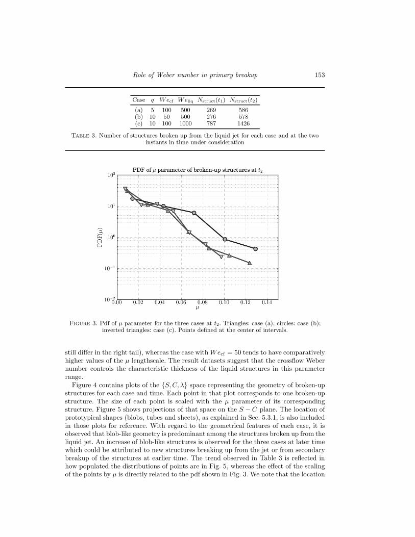
Figure 3 shows the probability density function of the µ parameter of the broken-upstructures. This parameter defines a characteristic lengthscale of the structure. For asphere, µ equals its radius, whereas for tubes and sheets, µtube ≈ 3 t/4 and µsheet ≈ t/2,respectively, where t is the thickness. Interestingly, Wecf has a dominant effect on thesepdfs. Both cases with Wecf = 100 show similar pdfs for a wide range of µ values (they


Case q Wecf Weliq Nstruct(t1) Nstruct(t2)

(a) 5 100 500 269 586(b) 10 50 500 276 578(c) 10 100 1000 787 1426

Table 3. Number of structures broken up from the liquid jet for each case and at the twoinstants in time under consideration

Figure 3. Pdf of µ parameter for the three cases at t2. Triangles: case (a), circles: case (b);inverted triangles: case (c). Points defined at the center of intervals.

still differ in the right tail), whereas the case with Wecf = 50 tends to have comparativelyhigher values of the µ lengthscale. The result datasets suggest that the crossflow Webernumber controls the characteristic thickness of the liquid structures in this parameterrange.

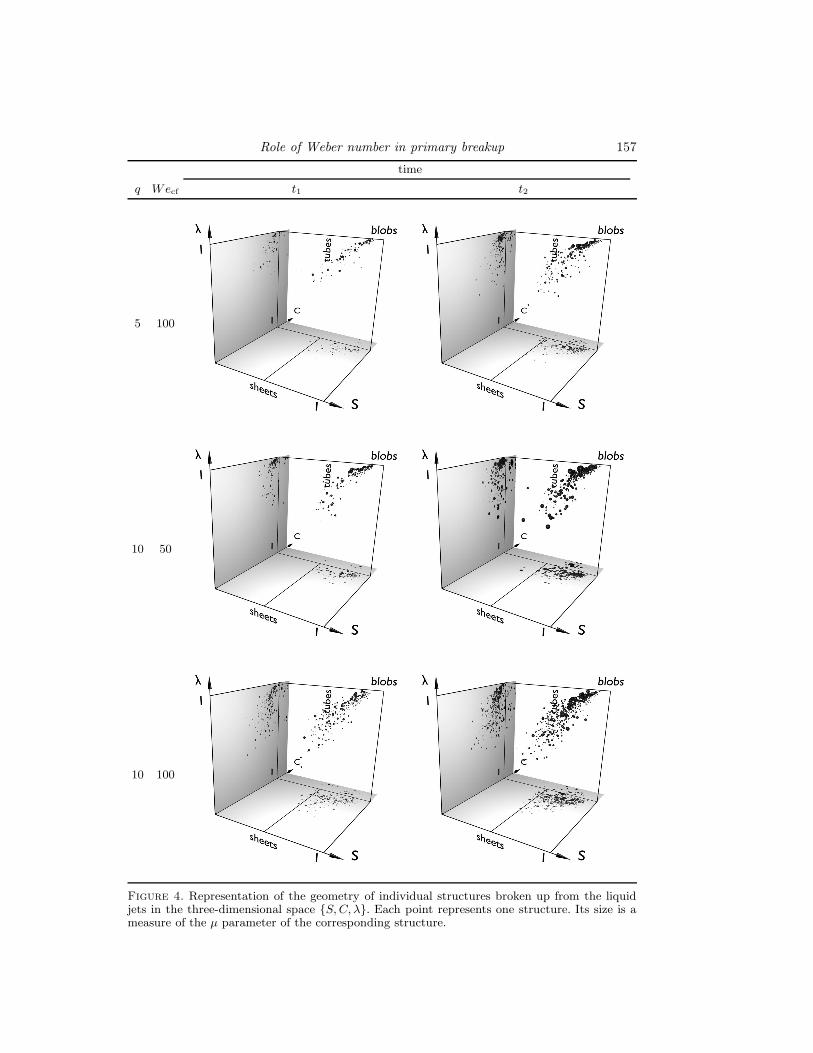
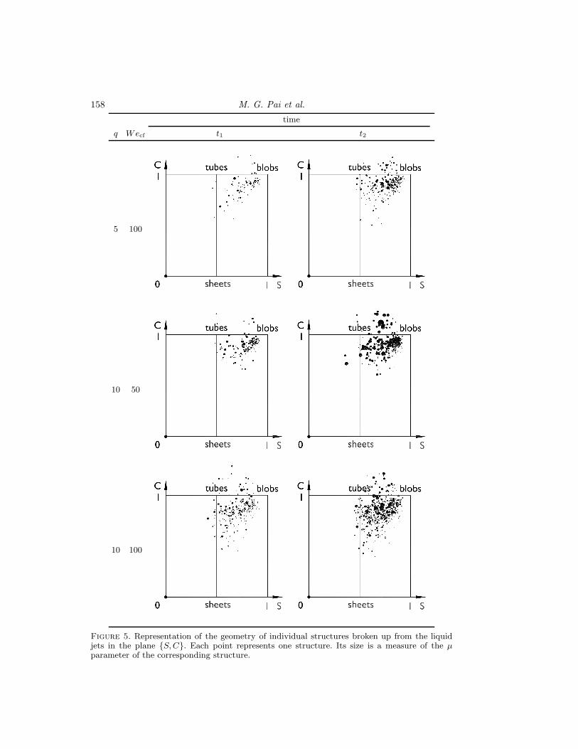
Figure 4 contains plots of the {S, C, λ} space representing the geometry of broken-upstructures for each case and time. Each point in that plot corresponds to one broken-upstructure. The size of each point is scaled with the µ parameter of its correspondingstructure. Figure 5 shows projections of that space on the S − C plane. The location ofprototypical shapes (blobs, tubes and sheets), as explained in Sec. 5.3.1, is also includedin those plots for reference. With regard to the geometrical features of each case, it isobserved that blob-like geometry is predominant among the structures broken up from theliquid jet. An increase of blob-like structures is observed for the three cases at later timewhich could be attributed to new structures breaking up from the jet or from secondarybreakup of the structures at earlier time. The trend observed in Table 3 is reflected inhow populated the distributions of points are in Fig. 5, whereas the effect of the scalingof the points by µ is directly related to the pdf shown in Fig. 3. We note that the location


of points in the {S, C, λ} space contains shape information that is independent of thesize of the structure, while the size of each point in that space is related to a lengthscaleof the structure, as defined above. The scaling is common to all plots, so that they canbe consistently compared. For instance, the presence of larger points in case (b) at t2indicates a tendency to higher values of µ as plotted in Fig. 3.

Case (c) (bottom panel in Figs. 4 and 5) shows a larger spread of geometrical shapesamong the three cases. In particular there are large structures with relatively low valuesof λ (i.e., considerable stretching). Also the value of C shows a higher variance, reachinglower values than for the other two cases. The combined effect of lower values of λ andC reflects a tendency toward sheet-like structures. These are less common for the othertwo cases. Despite some occurrences of structures approaching the sheet-like region, thistype of geometry is not as commonly encountered as blobs, tubes and the other shapes.

6. Conclusions and future work

The objective of this study was twofold. One was to ascertain the effect of meshresolution on the evolution of the LJCF. We notice that the mesh resolution does notaffect the wavelength of the liquid surface instabilities lending credence to our assumptionin Pai et al. (2009) that the coarse mesh resolution does not affect these statistics.The other objective involved using a differential geometry technique to analyze liquidstructures for their geometrical characteristics. In the earlier study (Pai et al. 2009),we provided evidence that the wavelength of liquid surface instabilities were controlledprimarily by the liquid Weber number. We further concluded by observing the liquidmass evolution that the smallest lengthscales of the liquid jet were controlled again bythe liquid Weber number. From the preliminary geometrical analysis of liquid structuresthat was performed in this study, intriguingly however it appears that the role of crossflowWeber number in the primary breakup of the liquid jet cannot be entirely discounted.For the parameters of the study, it appears that the crossflow Weber number controls thecharacteristic thickness of the liquid structures, while the shapes of the liquid structures,such as blobs, tubes or sheets, are controlled by the liquid Weber number. Yet we observethat the number of liquid structures produced at the same characteristic timescale iscontrolled by the liquid Weber number. This may point to an interesting mechanism ofbreakup of ligaments where the inertia in the liquid as characterized by the liquid Webernumber causes separated structures to break up further, with the characteristic thicknessof these structures being controlled by the crossflow Weber number.

Geometrical analyses such as the one presented in this study seem very appropriatefrom the purview of primary breakup modeling. The analysis presented in this studysuggests that it might not be sufficient for a primary breakup model to merely predicta size distribution of droplets. Such geometrical and statistical analyses using multipleindependent simulations of LJCF might reveal that a primary breakup model must cap-ture the presence of a certain proportion of separated structures (such as blobs, tubesand sheets), or model its effect on the size or volume distribution of separated struc-tures that it supplies to a secondary breakup model. Clearly, a primary breakup modelthat simply provides a distribution of spherical droplets without regard to the subtleprocesses involved during this stage of breakup cannot be expected to be predictive inrealistic simulations of gas-turbine combustors, where unsteadiness in both the liquid jetinjection and the crossflow can modify the primary breakup mechanisms. This might in


turn lead to drop size distributions after secondary breakup that can be very differentfrom experimentally measured distributions such as the log-normal distribution.

Ideally the simulations and the analyses presented in this study need to be extended toseveral tens of diameters downstream from the liquid injection, so that a comprehensiveanalysis of primary and secondary breakup of liquid jets may be performed. However,the immense computational cost prohibits such detailed numerical simulations from beingcarried out, at least at present. Such detailed numerical simulations need to be contrastedwith simulations that use the large-eddy simulation technique for the carrier phase. Fur-thermore, in such simulations small separated structures are converted to point particles.While these are attractive techniques to reduce computational expense, they add a levelof uncertainty and modeling into the entire breakup process which defeats the very pur-pose of performing detailed simulations in the first place. Findings from such analyseswill in turn depend on modeling parameters (such as the LES sub-grid models for boththe liquid and gas phase, the threshold below which a ligament is considered a pointparticle, etc.) and their effect on primary breakup processes identified in this study willneed to be precisely quantified.

Detailed numerical simulations are able to provide unique insight into the mechanismof breakup of a LJCF. Such simulations coupled with careful analyses such as the onepresented in this study can unravel intricacies and subtleties in liquid primary breakup,which was until now deemed to be controlled by a single parameter (for instance, thecrossflow Weber number is the principal non-dimensional group used in regime diagramsfor LJCF).

Acknowledgments

Funding from UTRC and NASA is acknowledged. Computational time for numericalsimulations were made available on TACC-Ranger and TACC-Spur at The University ofTexas, Austin, through a NSF compute time grant.

REFERENCES

Bellofiore, A. 2006 Experimental and numerical study of liquid jets injected in high-density air crossflow. PhD thesis, University of Naples.

Bermejo-Moreno, I. & Pullin, D. I. 2008 On the non-local geometry of turbulence.J. Fluid Mech. 603, 101–135.

Desjardins, O. 2008 Numerical methods for liquid atomization and application in de-tailed simulations of a diesel jet. PhD thesis, Stanford University.

Desjardins, O., Blanquart, G., Balarac, G. & Pitsch, H. 2008a High orderconservative finite difference scheme for variable density low Mach number turbulentflows. Journal of Computational Physics 227 (15), 7125–7159.

Desjardins, O., Moureau, V. & Pitsch, H. 2008b An accurate conservative levelset/ghost fluid method for simulating turbulent atomization. Journal of Computa-

tional Physics 227 (18), 8395–8416.

Desjardins, O. & Pitsch, H. 2009 A spectrally refined interface approach for simu-lating multiphase flows. Journal of Computational Physics 228 (5), 1658–1677.

Hieber, S. & Koumoutsakos, P. 2005 A Lagrangian particle level set method. Journal

of Computational Physics 210 (1), 342–367.


Hinze, J. 1955 Fundamentals of the hydrodynamic mechanism of splitting in dispersionprocesses. AIChE Journal 1 (3), 289–295.

Kang, M., Fedkiw, R. & Liu, X. 2000 A boundary condition capturing method formultiphase incompressible flow. Journal of Scientific Computing 15 (3), 323–360.

Lee, K., Aalburg, C., Diez, F., Faeth, G. & Sallam, K. 2007 Primary breakupof turbulent round liquid jets in uniform crossflows. AIAA journal 45 (8), 1907.

Lefebvre, A. 1998 Gas turbine combustion. CRC.

Muppidi, S. & Mahesh, K. 2007 Direct numerical simulation of round turbulent jetsin crossflow. Journal of Fluid Mechanics 574, 59–84.

Pai, M. G., Desjardins, O., & Pitsch, H. 2008 Detailed numerical simulations ofprimary breakup of liquid jets in crossflow. In Annual Research Briefs . Center forTurbulence Research.

Pai, M. G., Pitsch, H. & Desjardins, O. 2009 Detailed Numerical Simulations ofPrimary Atomization of Liquid Jets in Crossflow. In 47 th AIAA Aerospace Sciences

Meeting. American Institute of Aeronautics and Astronautics.

Sallam, K. A., Aalburg, C. & Faeth, G. 2004 Breakup of round nonturbulent liquidjets in gaseous crossflow. AIAA journal 42 (12), 2529–2540.

Scardovelli, R. & Zaleski, S. 1999 Direct numerical simulation of free-surface andinterfacial flow. Annual Review of Fluid Mechanics 31 (1), 567–603.

Sussman, M., Smith, K. M., Hussaini, M. Y., Ohta, M. & Zhi-Wei, R. 2007Direct numerical simulation of free-surface and interfacial flow. J. Comp. Physics

221, 469–505.


time

q Wecf t1 t2

5 100

10 50

10 100

Figure 4. Representation of the geometry of individual structures broken up from the liquidjets in the three-dimensional space {S, C, λ}. Each point represents one structure. Its size is ameasure of the µ parameter of the corresponding structure.


time

q Wecf t1 t2

5 100

10 50

10 100

Figure 5. Representation of the geometry of individual structures broken up from the liquidjets in the plane {S, C}. Each point represents one structure. Its size is a measure of the µparameter of the corresponding structure.

Documents

Center for Turbulence Research Annual Research Briefs 2009