Embed Size (px)
Citation preview
Federal Reserve Bank of Minneapolis Research Department
Catch-up Growth Followed by Stagnation: Mexico, 1950–2010
Timothy J. Kehoe and Felipe Meza
Working Paper 693
Revised November 2012
ABSTRACT___________________________________________________________________ In 1950 Mexico entered an economic takeoff and grew rapidly for more than 30 years. Growth stopped during the crises of 1982–1995, despite major reforms, including liberalization of foreign trade and investment. Since then growth has been modest. We analyze the economic history of Mexico 1877–2010. We conclude that the growth 1950–1981 was driven by urbanization, industrialization, and education and that Mexico would have grown even more rapidly if trade and investment had been liberalized sooner. If Mexico is to resume rapid growth — so that it can approach U.S. levels of income — it needs further reforms. JEL classification: N16, O11, O54, Key words: Mexico, economic growth, total factor productivity. ______________________________________________________________________________ * Kehoe: University of Minnesota, Federal Reserve Bank of Minneapolis, and National Bureau of Economic Research; Meza: Instituto Tecnológico Autónomo de México. Kehoe’s work was undertaken with the support of the National Science Foundation under grant SES-09-62865. Meza thanks CONACYT via research grant 81825 and the Asociación Mexicana de Cultura A.C. for support. We thank Alejandro Hernández, Kim Ruhl, Jaime Serra-Puche, and participants at the conference on “Economic Growth: Latin America at its Bicentennial Celebration” at the Pontificia Universidad Católica de Chile, December 2010, especially Juan Pablo Nicolini and the organizers, Raimundo Soto and Felipe Zurita, for helpful comments. José Asturias and Sewon Hur provided extraordinary research assistance. The data used in this paper are available at www.econ.umn.edu/~tkehoe. The views expressed herein are those of the authors and not necessarily those of the Federal Reserve Bank of Minneapolis or the Federal Reserve System.
1
1. Introduction
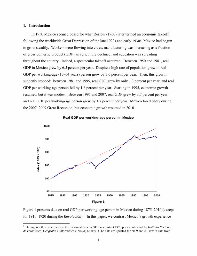
In 1950 Mexico seemed posed for what Rostow (1960) later termed an economic takeoff:
following the worldwide Great Depression of the late 1920s and early 1930s, Mexico had begun
to grow steadily. Workers were flowing into cities, manufacturing was increasing as a fraction
of gross domestic product (GDP) as agriculture declined, and education was spreading
throughout the country. Indeed, a spectacular takeoff occurred: Between 1950 and 1981, real
GDP in Mexico grew by 6.5 percent per year. Despite a high rate of population growth, real
GDP per working-age (15–64 years) person grew by 3.6 percent per year. Then, this growth
suddenly stopped: between 1981 and 1995, real GDP grew by only 1.3 percent per year, and real
GDP per working-age person fell by 1.6 percent per year. Starting in 1995, economic growth
resumed, but it was modest: Between 1995 and 2007, real GDP grew by 3.7 percent per year
and real GDP per working-age person grew by 1.7 percent per year. Mexico fared badly during
the 2007–2009 Great Recession, but economic growth resumed in 2010.
Real GDP per working-age person in Mexico
-1.00
0.00
1.00
2.00
3.00
4.00
1875 1890 1905 1920 1935 1950 1965 1980 1995 2010
ind
ex
(1
87
5 =
10
0)
100
200
400
800
1600
50
Figure 1.
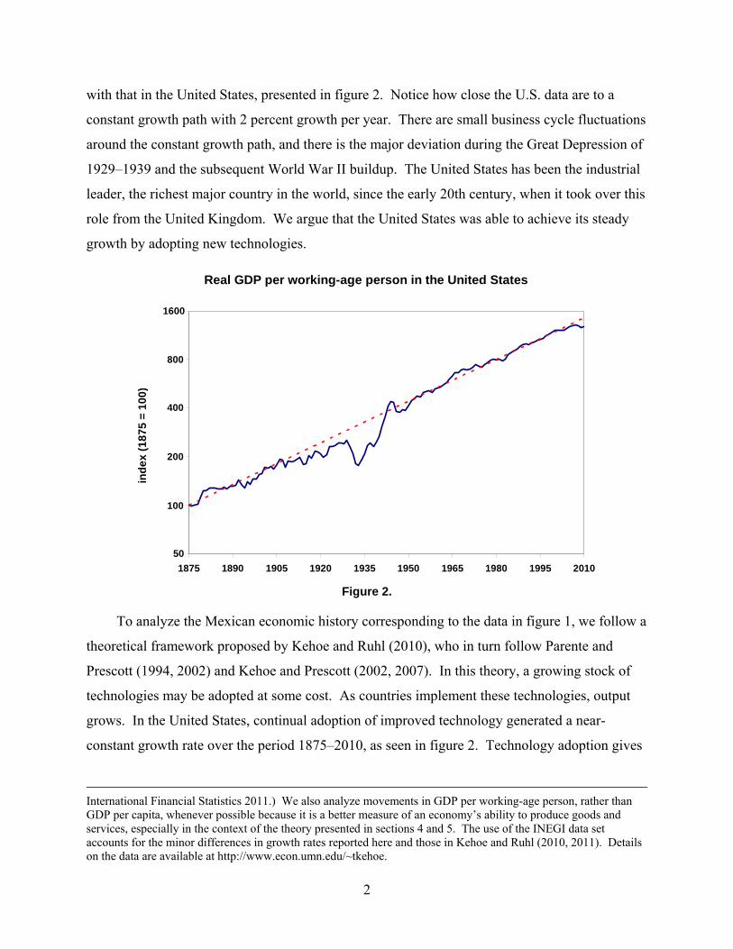
Figure 1 presents data on real GDP per working-age person in Mexico during 1875–2010 (except
for 1910–1920 during the Revolución).1 In this paper, we contrast Mexico’s growth experience
1 Throughout this paper, we use the historical data on GDP in constant 1970 prices published by Instituto Nacional de Estadística, Geografía e Informática (INEGI) (2009). (The data are updated for 2009 and 2010 with data from
2
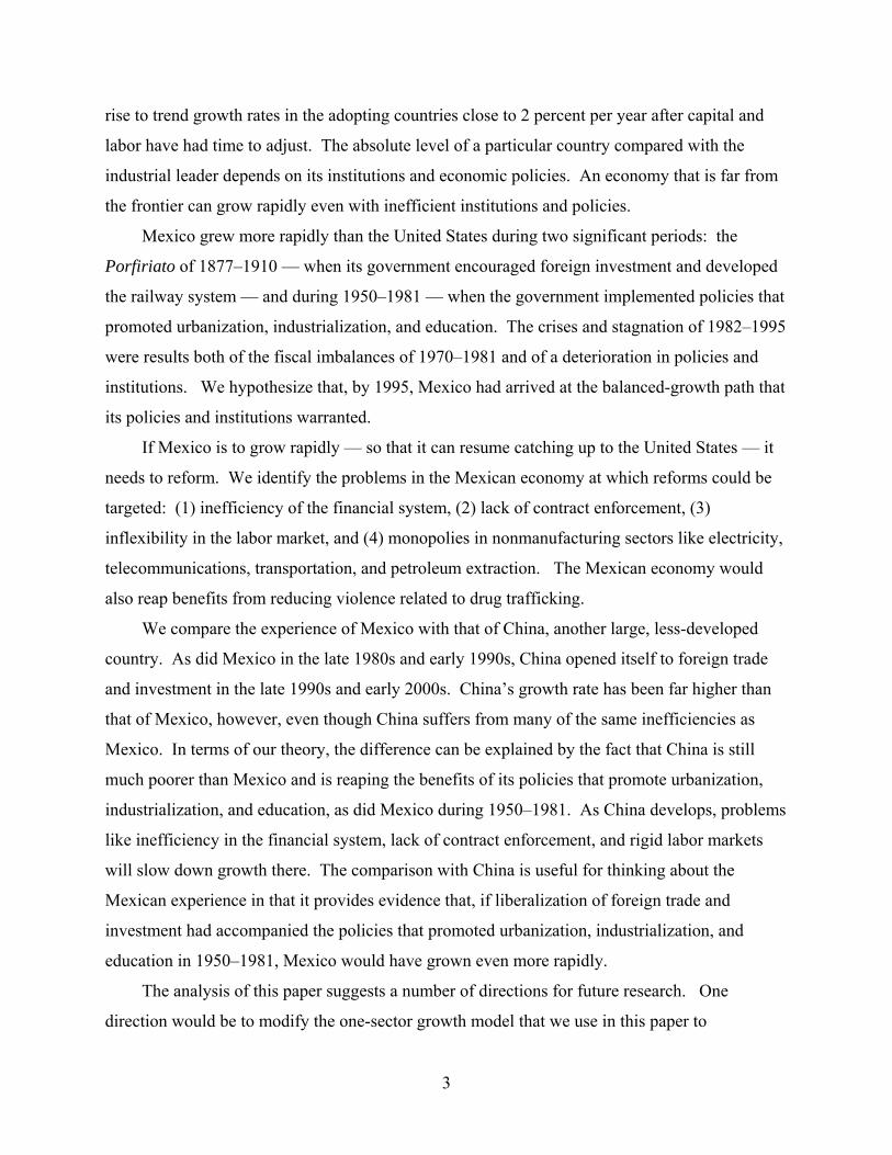
with that in the United States, presented in figure 2. Notice how close the U.S. data are to a
constant growth path with 2 percent growth per year. There are small business cycle fluctuations
around the constant growth path, and there is the major deviation during the Great Depression of
1929–1939 and the subsequent World War II buildup. The United States has been the industrial
leader, the richest major country in the world, since the early 20th century, when it took over this
role from the United Kingdom. We argue that the United States was able to achieve its steady
growth by adopting new technologies.
Real GDP per working-age person in the United States
-1.00
0.00
1.00
2.00
3.00
4.00
1875 1890 1905 1920 1935 1950 1965 1980 1995 2010
ind
ex
(1
87
5 =
10
0)
100
200
400
800
1600
50
Figure 2.
To analyze the Mexican economic history corresponding to the data in figure 1, we follow a
theoretical framework proposed by Kehoe and Ruhl (2010), who in turn follow Parente and
Prescott (1994, 2002) and Kehoe and Prescott (2002, 2007). In this theory, a growing stock of
technologies may be adopted at some cost. As countries implement these technologies, output
grows. In the United States, continual adoption of improved technology generated a near-
constant growth rate over the period 1875–2010, as seen in figure 2. Technology adoption gives
International Financial Statistics 2011.) We also analyze movements in GDP per working-age person, rather than GDP per capita, whenever possible because it is a better measure of an economy’s ability to produce goods and services, especially in the context of the theory presented in sections 4 and 5. The use of the INEGI data set accounts for the minor differences in growth rates reported here and those in Kehoe and Ruhl (2010, 2011). Details on the data are available at http://www.econ.umn.edu/~tkehoe.
3
rise to trend growth rates in the adopting countries close to 2 percent per year after capital and
labor have had time to adjust. The absolute level of a particular country compared with the
industrial leader depends on its institutions and economic policies. An economy that is far from
the frontier can grow rapidly even with inefficient institutions and policies.
Mexico grew more rapidly than the United States during two significant periods: the
Porfiriato of 1877–1910 — when its government encouraged foreign investment and developed
the railway system — and during 1950–1981 — when the government implemented policies that
promoted urbanization, industrialization, and education. The crises and stagnation of 1982–1995
were results both of the fiscal imbalances of 1970–1981 and of a deterioration in policies and
institutions. We hypothesize that, by 1995, Mexico had arrived at the balanced-growth path that
its policies and institutions warranted.
If Mexico is to grow rapidly — so that it can resume catching up to the United States — it
needs to reform. We identify the problems in the Mexican economy at which reforms could be
targeted: (1) inefficiency of the financial system, (2) lack of contract enforcement, (3)
inflexibility in the labor market, and (4) monopolies in nonmanufacturing sectors like electricity,
telecommunications, transportation, and petroleum extraction. The Mexican economy would
also reap benefits from reducing violence related to drug trafficking.
We compare the experience of Mexico with that of China, another large, less-developed
country. As did Mexico in the late 1980s and early 1990s, China opened itself to foreign trade
and investment in the late 1990s and early 2000s. China’s growth rate has been far higher than
that of Mexico, however, even though China suffers from many of the same inefficiencies as
Mexico. In terms of our theory, the difference can be explained by the fact that China is still
much poorer than Mexico and is reaping the benefits of its policies that promote urbanization,
industrialization, and education, as did Mexico during 1950–1981. As China develops, problems
like inefficiency in the financial system, lack of contract enforcement, and rigid labor markets
will slow down growth there. The comparison with China is useful for thinking about the
Mexican experience in that it provides evidence that, if liberalization of foreign trade and
investment had accompanied the policies that promoted urbanization, industrialization, and
education in 1950–1981, Mexico would have grown even more rapidly.
The analysis of this paper suggests a number of directions for future research. One
direction would be to modify the one-sector growth model that we use in this paper to

4
incorporate multiple sectors and to formalize Rostow’s (1960) concept of stages of growth.
Another, related, direction would be to use an open economy model to quantify the costs and
benefits of import substitution during Mexico’s rapid growth of 1950–1981.
2. Economic history up until 1950
Mexico’s economic history from Independence in 1810 until the first inauguration of
Porfirio Díaz as president in 1877 did not involve much economic growth. The period 1810–
1877 was one of political instability. Between 1833 and 1855, for example, Antonio López de
Santa Anna was president during 11 nonconsecutive periods. Mexico suffered from major
military invasions by the United States in 1847–1848 and by France in 1862–1867. Real GDP
per capita fell during the period 1810–1877 by a cumulative 10.5 percent.
Mexican economic history, 1877–2010
-1.00
0.00
1.00
2.00
3.00
4.00
1875 1890 1905 1920 1935 1950 1965 1980 1995 2010
ind
ex
(1
87
7 =
10
0)
Porfiriato
Revoluciónand
reconstruction
Great Depression
and recovery
Import substitution
and catch-up growth
Crisis and
reform
Fiscal imbalances
and collapse of import
substitution
Recovery and
slow growth
100
200
400
800
1600
50
Great Recession
Figure 3.
We date the modern economic history of Mexico as beginning in 1877, with the first
inauguration of Porfirio Díaz. We divide 1877–2010 into the periods in figure 3. In this section,
we examine economic events that took place during 1877–1950, which set the stage for the
takeoff experienced by the Mexican economy starting in 1950. Our principal source is Solís
(2000).
5
2.1. 1877–1910: Porfiriato
Porfirio Díaz was president of Mexico during 1877–1880 and 1884–1911. The Revolución,
the Mexican civil war that started in 1910, grew out of widespread social discontent with the
Díaz regime. At the beginning of the Porfiriato, the economic geography of Mexico could be
described as a collection of small economic units that functioned in an autarkic way, producing
goods for self-consumption. The most important economic feature of the Porfiriato was the
construction of railroads. Mexico became a nationwide market economy as the possibilities of
exchange grew. In parallel, there were major investments in ports, telegraph, telephone, and
electricity. The government played an important role in promoting foreign investment in
railroads. The government granted concessions and paid subsidies per kilometer of railway built.
The principal source of funds for the construction of the railways was American investors.
When Díaz came to power in 1877 Mexico had 640 km of railways. During his first term
as president, railways grew to a total of 1,074 km. Between 1880 and 1884, railways grew to a
total of 5,731 km. As a result, Mexico had railways going from Mexico City to Veracruz, the
main port in the Gulf of Mexico, and to the border with the United States. Railways went from
5,731 km to 19,748 km from 1884 to 1910. The expansion of railways had many effects on the
Mexican economy. Exporting firms (raw materials from mining being the principal Mexican
export) saw their costs reduced. Internal migration of workers, as a function of regional
differences in wages, grew. New mining projects were undertaken, as the fall in transport costs
made them profitable.
Economic growth in Mexico during the Porfiriato was impressive for that time: real GDP
per capita grew by 2.1 percent per year during 1877–1910. According to Rostow (1960), modern
economic growth started in the United Kingdom in the early 19th century, and, according to
Maddison (1995), in the United Kingdom the average growth of real GDP per capita 1820–1900
was 1.2 percent per year. Between 1875 and 1910, real GDP per capita in the United States grew
by 2.0 per year, as the United States overtook and passed the United Kingdom, whose growth
rate during this period was only 0.9 percent per year, to become the world’s industrial leader.
During this period, Mexico, whose growth rate was 2.1 percent per year, grew even faster. As
the data in figure 4 illustrate, the Porfiriato was the period — except for the 1950–1981 import

6
substitution period — in which Mexico was catching up to the United States.2 We interpret the
economic events of the Porfiriato as the beginning of an economic takeoff that was aborted by
the events of the Revolución and the worldwide Great Depression that followed shortly after.
20
25
30
35
40
45
50
1875 1890 1905 1920 1935 1950 1965 1980 1995 2010
per
cen
t
Real GDP per working-age person in Mexico compared to United States
Figure 4.
2.2. 1910–1928: Revolución and reconstruction
The Revolución, or civil war, that started in Mexico in 1910 as Francisco I. Madero led an
uprising against Porfirio Díaz, resulted in a large fall in the population and a large destruction of
the capital stock. The population of Mexico fell from 15.2 million to 14.3 million between 1910
and 1921, the period during which most of the armed conflict took place. Besides the reduction
in population caused directly by the war, there was a large migration to the United States.
According to Solís (2000), between 1910 and 1930, 600,000 Mexicans migrated. Another factor
behind the fall in population was the flu epidemic 1918–1919. The migration to the United
States and the flu epidemic must have disproportionately affected people with low education
levels. According to census data, the number of people who knew how to read and write rose
from 3.0 million in 1910 to 3.6 million in 1921, even as the overall population fell.
2 The data in figure 4 differ from those in figures 1 and 2 and those used in the rest of the paper except in figure 18. They are purchasing power parity real GDP numbers taken from Maddison (2010) and the World Bank World Development Indicators (2011).
7
Álvaro Obregón, president from 1920 to 1924, oversaw the beginning of the reconstruction
of Mexico after the end of the armed conflict. There was an increase in investment in public
education. At the same time, however, the economic situation was characterized by high
uncertainty. For example, Obregón was not initially recognized as president by the United
States. Plutarco E. Calles, president from 1924 to 1928 — and one of the most important figures
in Mexican politics between 1924 and 1936 — created institutions that contributed to economic
development. In 1925, he created the Comisión Nacional de Caminos, which had the objective
of expanding Mexico’s road system. In the same year, Calles created the Banco de México,
Mexico’s central bank. Also in 1925, Calles created the Comisión Nacional de Irrigación, which
was responsible for carrying on large hydraulic projects for irrigation for the agricultural sector.
Growth was lower in this period than during the Porfiriato, as is to be expected. Real GDP
per working-age person grew at 0.4 percent per year. One important change with respect to the
Porfiriato is that the 1917 Constitution established the national interest in Mexico´s natural
resources. The 1938 nationalization of the oil industry, in which there was an important amount
of foreign investment, would reflect that interest in the coming decades.
2.3. 1928–1950: Great Depression and recovery
The worldwide Great Depression had a large negative impact on economic activity in
Mexico. In 1934, GDP per working-age person reached its lowest value since the end of the
19th century. Between 1928 and 1932, real GDP per working-age person fell by 7.0 percent per
year. Exports and imports fell. Given that a large fraction of tax revenues came from tariffs on
foreign trade, tax revenue fell 25 percent. Fiscal expenditures were reduced.
Following the Depression, Mexico started growing again. Important institutions were
created. In terms of politics, military leaders started losing ground to civilian leaders. Industrial
workers and farmers were incorporated to the political system, through the Partido
Revolucionario Institucional (PRI), which governed Mexico until the end of the 20th century.
Four important events took place in the interwar period: the nationalization of the oil industry,
the development of the financial system, expenditure on public investment, and the agrarian
reform.
The nationalization of the oil industry in 1938 had as a major consequence import
substitution, as products that were previously imported were now produced domestically.

8
According to Solís (2000), in broader terms, the management of the oil industry was now aimed
at contributing to the development of the economy.
The financial system recovered after the contraction suffered during the Revolución. Bank
assets were one-third of GDP in 1910. In 1925, they were one-fifth. Bank assets recovered their
pre-Revolución level in 1940. Banking credit also fell during this period. During the Revolución
there was an increase in currency in circulation and in inflation. It is important to note that one
of the main characteristics of the Banco de México was that it was granted the monopoly over
currency emission. Before this event, private banks could print money. Inflation during the
Revolución led to the use of the dollar in the northern part of the country, and in Veracruz and
Tampico. Coins with gold or silver content that had been hoarded started being used in
transactions. After the creation of the Banco de México there was an increase in checking
accounts between 1925 and 1930. The Great Depression brought a fall in the price level and in
the money supply defined as medios de pago (M1). This happened until 1935, when both
variables started growing again. Between 1929 and 1934, the GDP deflator fell at an average
rate of 2.5 percent per year. The money supply as a percentage of GDP fell at an average rate of
3.5 per year.
The composition of government expenditure shifted during 1934–1952. During the
administration of Lázaro Cárdenas (president during 1934–1940), expenditures on irrigation,
credit to the agricultural sector, communications, and public works increased from 20–25 percent
to 37–40 percent of the public budget. Presidents Ávila Camacho and Alemán maintained this
trend. By 1952, these sorts of expenditures represented 46.9 percent of the budget. Additionally,
during the Cárdenas administration, expenditures on education, public health, water provision,
and sewage increased, reaching 19.9 percent of the budget, a maximum until 1962.
The Reforma Agraria was aimed at distributing land to peasants. This was one of the
principal demands of peasants during the Revolución. The Obregón and Calles administrations
had started distributing land through institutional channels. During the Cárdenas administration,
this process accelerated. Cárdenas distributed 18.8 million hectares. Both President Ávila
Camacho and President Alemán carried on this policy, at a slower pace, distributing 7.3 and 4.6
million hectares, respectively. During the Great Depression there was a fall in output in the
agricultural sector. According to Solís (2000), during the period 1929–1950, real GDP (at 1960
9
pesos) in the agricultural sector grew at an average rate of 3.9 percent per year, which is almost
the same growth of total GDP, which was 4.0 percent per year.
Over the entire 1928–1950 period, real GDP per working-age person grew at 1.3 percent
per year. This is the combination of the fall of 7.0 percent per year 1928–1932 with a recovery
at a rate of 3.7 percent per year 1932–1950. The data in figure 4 show that the recovery in
Mexico was not as vigorous as that in the United States, however. According to Solís (2000),
during the period 1929–1950 average yearly inflation, measured with the GDP deflator, was
relatively high, at 6.5 percent per year. It was 9.5 percent per year between 1934 and 1950.
3. Economic history since 1950
In terms of Rostow’s (1960) stages of economic growth, we can think of Mexico as starting
a takeoff during the Porfiriato, only to have it aborted by the events connected with the
Revolución and the Great Depression. The recovery following the Great Depression set the stage
for the takeoff that occurred in the three decades after 1950. We view the takeoff as the product
of urbanization and industrialization and the increase in education levels, as well as the adoption
of advanced technologies from abroad, principally the United States. Our sources are Cárdenas
(1996) and Solís (2000). In this section, we analyze this experience as well as the slowdown
that has followed.
3.1. 1950–1970: Import substitution and catch-up growth
Capital accumulation grew during the 1950s. During the 1950s, total investment grew
faster than GDP. The government invested in public infrastructure: the oil industry, highways,
health, and education. In terms of the loanable funds for investment emphasized by Rostow
(1960), it is worth stressing that the private domestic financial system was a limited source for
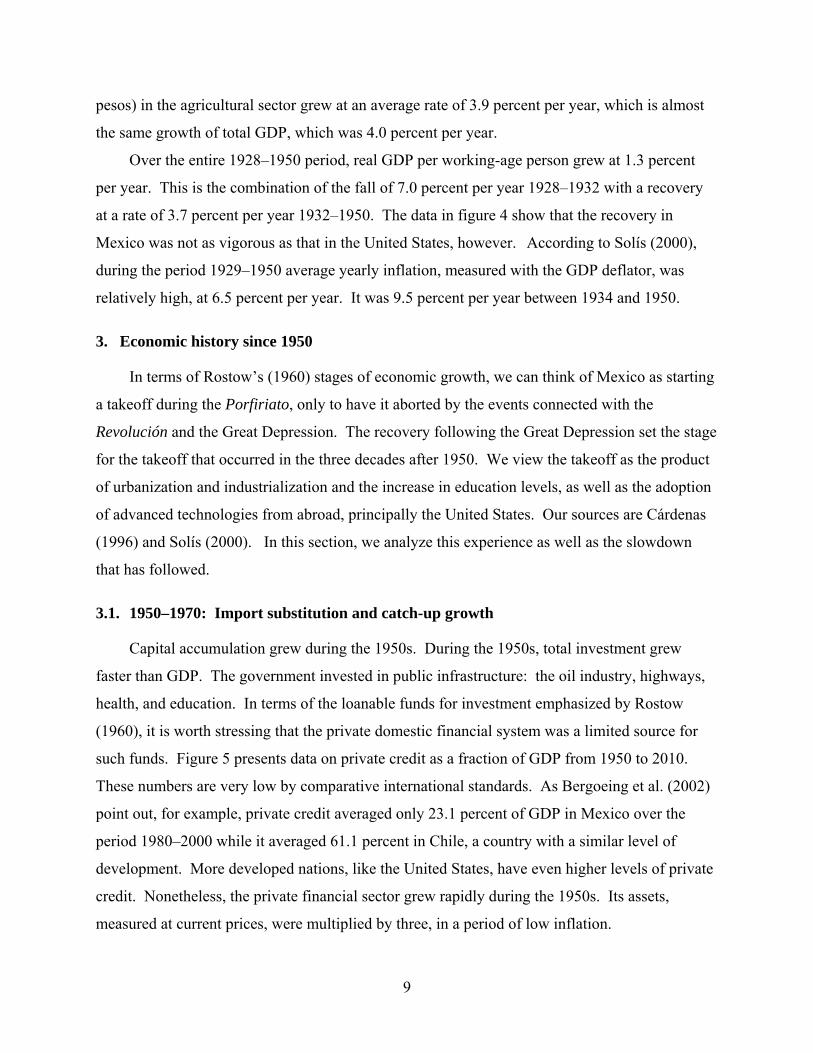
such funds. Figure 5 presents data on private credit as a fraction of GDP from 1950 to 2010.
These numbers are very low by comparative international standards. As Bergoeing et al. (2002)
point out, for example, private credit averaged only 23.1 percent of GDP in Mexico over the
period 1980–2000 while it averaged 61.1 percent in Chile, a country with a similar level of
development. More developed nations, like the United States, have even higher levels of private
credit. Nonetheless, the private financial sector grew rapidly during the 1950s. Its assets,
measured at current prices, were multiplied by three, in a period of low inflation.
10
Private credit in Mexico
10
15
20
25
30
35
40
1950 1960 1970 1980 1990 2000
pe
rce
nt
GD
P
Figure 5.
During this period, the growth of the agricultural sector was related to industrialization.
Between 1945 and 1952, the agricultural sector grew more because of the extensive margin than
because of a higher yield by hectare. The situation reversed between 1952 and 1956. This was
due to a larger domestic and external demand, the growth of cities, and the process of
industrialization. Industries demanded goods such as cotton.
After a balance of payments crisis in 1948, the government decided to protect the domestic
production of consumption goods and imposed import quotas. The government also provided
fiscal measures to foster the reinvestment of profits, and kept and expanded the policy of creation
of new firms through subsidies, fiscal exemptions, and the support of Nacional Financiera, the
largest of the government-operated development banks.
In 1950, for a large set of goods, there was no import substitution, as domestic industries
already satisfied 95 percent of the domestic market for such products as textiles, food, beverages,
and tobacco (classified as basic industries), shoes and soap (classified as consumption goods),
and rubber, alcohol, and glass (classified as intermediate goods). For other products, there was a
significant amount of import substitution. These goods were intermediates, durables, and capital
goods. Cárdenas (1996) decomposes the sources of growth of industrial demand into domestic
demand, external demand, import substitution, and structural change. Between 1950 and 1954,

11
he finds that import substitution was negligible. Between 1954 and 1958 its contribution was 9
percent, a contribution smaller than in the 1930s. It is interesting to note that, between 1952 and
1958, 38 percent of private investment was destined to the purchase of imported machinery and
equipment. In this sense, there was substantial technology adoption from abroad in that period.
According to Cárdenas (1996), during the period 1958–1962, the contribution of import
substitution to the growth of industrial demand was 22.3 percent due to a more protectionist trade
policy. Over time, import substitution became difficult because it had to take place by producing
intermediate and capital goods. Figure 6 presents data on the evolution of foreign trade in
Mexico.
International trade in Mexico
10
20
30
40
50
60
70
1950 1960 1970 1980 1990 2000 2010
pe
rce
nt
GD
P
Figure 6.
The increase in GDP took place at the same time as urban growth. Figure 7 presents data
on urbanization. Here the urban population is defined as that living in agglomerations of more
than 2,500 inhabitants. Similar graphs are obtained for other definitions of urban population, but
there are more data for this definition. There was also a reduction in the size of the agricultural
sector and of mining. Figure 8 presents data on the sectoral composition of GDP. Migration
from rural to urban areas was due to a lack of opportunities in the agricultural sector. The
capital-labor ratio grew 7 percent on average during this period, which increased real wages.

12
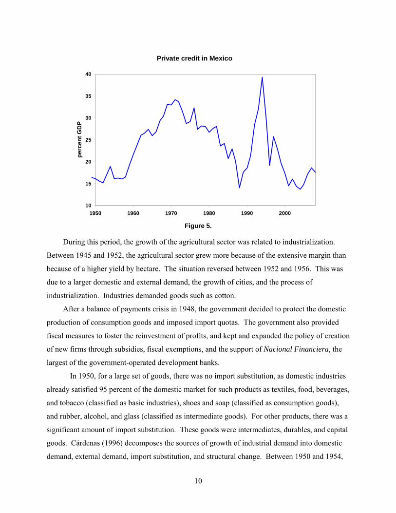
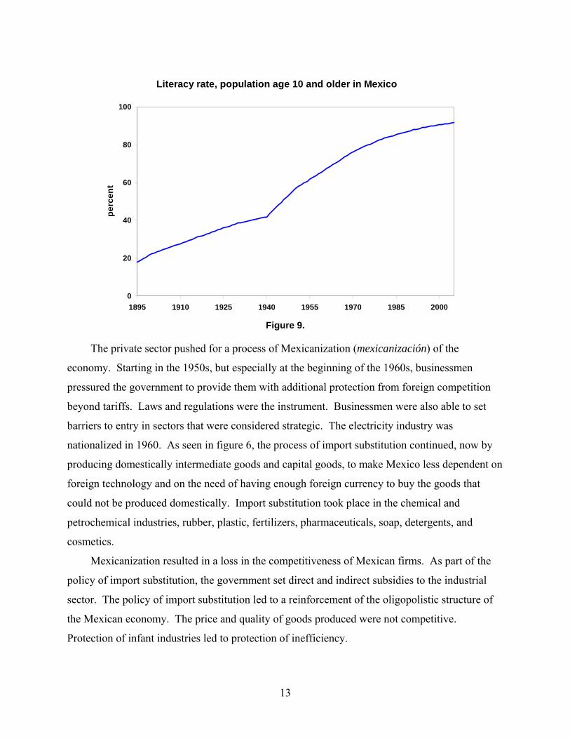
Gross fixed capital formation grew at 10.3 percent between 1963 and 1970, increasing the
investment to GDP ratio to 18.5 percent in 1970. Figure 9 shows the rapid spread of literacy.
Urban population in Mexico
20
30
40
50
60
70
80
1900 1920 1940 1960 1980 2000
pe
rce
nt
Figure 7.
Composition of GDP in Mexico
0
10
20
30
40
50
60
70
1950 1960 1970 1980 1990 2000
pe
rce
nt
services
manufacturing
agriculture
Figure 8.
13
Literacy rate, population age 10 and older in Mexico
0
20
40
60
80
100
1895 1910 1925 1940 1955 1970 1985 2000
pe
rce
nt
Figure 9.
The private sector pushed for a process of Mexicanization (mexicanización) of the
economy. Starting in the 1950s, but especially at the beginning of the 1960s, businessmen
pressured the government to provide them with additional protection from foreign competition
beyond tariffs. Laws and regulations were the instrument. Businessmen were also able to set
barriers to entry in sectors that were considered strategic. The electricity industry was
nationalized in 1960. As seen in figure 6, the process of import substitution continued, now by
producing domestically intermediate goods and capital goods, to make Mexico less dependent on
foreign technology and on the need of having enough foreign currency to buy the goods that
could not be produced domestically. Import substitution took place in the chemical and
petrochemical industries, rubber, plastic, fertilizers, pharmaceuticals, soap, detergents, and
cosmetics.
Mexicanization resulted in a loss in the competitiveness of Mexican firms. As part of the
policy of import substitution, the government set direct and indirect subsidies to the industrial
sector. The policy of import substitution led to a reinforcement of the oligopolistic structure of
the Mexican economy. The price and quality of goods produced were not competitive.
Protection of infant industries led to protection of inefficiency.
14
The government pursued a policy of Mexicanization of production, and to create empresas
paraestatales, firms run by the government, based on the belief that it was better to borrow from
abroad than to accept foreign direct investment (FDI), as during the Porfiriato. In 1961, a new
mining law stated that fiscal incentives would be given only to firms in which the majority of
capital was owned by Mexican nationals. New mining concessions would be granted to firms
with 66 percent national capital. The low production of iron, steel and sulfur led the government
to invest in their production. In the case of the petrochemical industry, the maximum percentage
of foreign capital was 40 percent. In 1966 the financial sector was Mexicanized. In 1970 the
government decided to Mexicanize the iron and steel industry, cement, glass, cellulose,
fertilizers, and aluminum. At least 51 percent of capital had to belong to nationals. This measure
was not retroactive, but existing foreign firms that planned to expand their plans or acquire new
ones had to be authorized by the Secretaría de Relaciones Exteriores (Department of Foreign
Affairs). Additionally, the use of Mexican intermediate goods was required in many sectors, in
particular in the production of cars, trucks and other durable goods. Mexican entrepreneurs were
protected not only from foreign products, but also from foreign capital.
3.2. 1970–1981: Fiscal imbalances and collapse of import substitution
The first half of this period, 1970–1976, was called Desarrollo Compartido (Shared
Development). The goals of economic policy announced in 1970 were economic growth and an
improvement of income distribution. The period known as Desarrollo Estabilizador (Stabilizing
Development), 1958–1970, according to Solís (2000) had been one of growth, but there was a
new objective: to reduce income inequality.
Between 1970 and 1981, the principal policy instrument was government spending. The
government incurred deficits that were financed via domestic credit from the Banco de México
and borrowing from abroad. The average yearly growth rate of the medios de pago (M1) was
25.8 percent between 1970 and 1982. Inflation was on average 18.9 percent per year, measured
with the GDP deflator. Real GDP per working-age person grew at an average rate of 3.5 percent.
Government intervention in the economy had a negative impact on the economy. There
was an increase in regulation and bureaucracy that discouraged the formation of new firms. The
creation of firms managed by the government, and the purchase of firms by the government,
increased the fiscal deficit. These firms represented projects of low social benefit. The economy
15
was also hit by external shocks, such as the fall in the price of oil in international markets, and
the rise in international interest rates, before the 1982 debt crisis.
During the administration of Luís Echeverría (1970–1976), public sector deficit as a
fraction of GDP went from 2.2 percent in 1970 to 9.0 percent in 1975. As the government
borrowed in international markets to finance the public sector deficit, the current account deficit
went from 1.8 percent of GDP in 1972 to 4.8 percent in 1975. The administration of Echeverría
ended with a devaluation of the peso after 22 years of fixing the exchange rate at 12.50 pesos per
dollar.
During the administration of José López Portillo (1976–1982), the discovery of massive oil
fields in early 1978 had a significant impact on economic policy. According to Cárdenas (1996),
proven oil reserves increased 151.2 percent between 1977 and 1978. The government
implemented a program of public investment aimed at the expansion of the oil industry. There
was also an expansion of public infrastructure and of provision of public health and education
services. Between 1978 and 1982, public investment and private investment grew in real terms at
a yearly rate of 15.0 percent. For the first time in history, the demand for elementary school
education was fully satisfied. The fraction of the population with access to medical services
reached 85 percent, having been 60 percent in 1976. The government created important policy
instruments. It implemented the VAT (IVA, Impuesto al Valor Agregado, Value-Added Tax). It
also created what would become the most important government domestic bonds, CETES
(Certificados de la Tesorería de la Federación).
The fall in the price of oil in mid-1981 had a severe negative impact on public finances. The
public sector deficit relative to GDP had reached a level of 10 percent in 1976, although it fell to
7 percent in 1980. The fall in oil exports in 1981 led to a deficit of 14.7 percent in 1981,
however, and to 17.6 percent in 1982. At the same time, the foreign debt of the public sector
went from 4.3 billion U.S. dollars in 1970 to 58.9 billion in 1982. Finally, in 1982, the Mexican
government announced that it could not face the scheduled debt payments, thus starting the 1982
debt crisis.
3.3. 1982–1995: Crisis and reform
In 1982, the macroeconomic situation in Mexico was difficult. The public sector deficit
was 17.6 percent of GDP. The current account deficit was 4 percent of GDP. Inflation,
16
measured with the GDP deflator, was 61.0 percent between 1981 and 1982. GDP per working-
age person fell 3.2 percent between 1981 and 1982, and 6.0 percent between 1982 and 1983.
The administration of Miguel de la Madrid (1982–1988) responded by setting up an economic
program known as Programa Inmediato de Reordenación Económica (PIRE), to be in place
between December 1982 and May 1986. The objectives of the program included reducing the
growth of public expenditure, carrying out public infrastructure projects, and honoring the
payments of external debt.
In terms of fiscal policy, the government reduced its expenditure, modified tax codes to
increase tax revenue, increased the prices of goods controlled by the government (that is, energy
prices such as the price of gasoline), and started a process of privatization of firms owned by the
government (the empresas paraestatales). The process of privatization was important. In 1982
there were 1,155 firms owned by the government. By 1988 there were 618 of these firms. The
privatization process would continue during 1988–1994. The nationalization of the banking
sector was a source of resources for the government. According to Aspe (1993), a major source
of resources was the encaje legal, which represented credit to the public sector at zero cost or at
low interest rates. In 1986 Mexico signaled its intention to open its markets to foreign
competition by joining the General Agreement on Tariffs and Trade (GATT). Inflation was
high despite the PIRE. Between 1986 and 1987, inflation, measured with the GDP deflator, was
141.0 percent.
In December 1987 a new economic program was created, the Pacto de Solidaridad
Económica (PSE), that had as its main objective the reduction of inflation. This program was in
effect until late 1988. The measures taken by the government included a reduction in the public
sector deficit, trade openness, and consensus building (concertación). The aim of consensus
building was to stabilize the price level. The government held meetings with labor union leaders
(sector obrero), peasant leaders (sector campesino), and businessmen. Workers reduced their
demands for increases in wages, peasants agreed not to increase guaranteed prices (precios de
garantía) in real terms, and businessmen agreed to reduce increases in prices and increase
productivity. In turn, the public sector agreed to reduce its expenditure and the number of firms
owned by the government. The public sector deficit went from 16.1 percent of GDP to 11.7
percent between 1987 and 1988. Inflation fell, but it remained at a high level.
17
In December of 1988, the administration of Carlos Salinas (1988–1994) created a new
program called the Pacto para la Estabilidad y el Crecimiento Económico (PECE). The
principal goal was to achieve an inflation rate of one digit by reaching a consensus with workers
and businessmen. The public sector balance was actually a surplus in 1991 and remained a
surplus until the end of the Salinas government. The program was successful as inflation fell
from 141.0 percent in 1987 to 8.3 percent in 1994.
Many reforms took place during 1988–1994: among them, a continued privatization of
firms owned by the government, the signing of the North American Free Trade Agreement
(NAFTA), the liberalization of the banking sector, and the independence of the central bank,
Banco de México. The process of regaining access to international financial markets, after the
1982 debt crisis, was also undertaken. The number of firms owned by the government that were
privatized went from 618 in 1988 to 252 in 1994. An important firm privatized in this period
was TELMEX, the monopoly providing telephone services.
In May 1990 the government announced its intention to sign a trade agreement with the
United States. In January 1994 NAFTA, the trade and foreign investment agreement with the
United States and Canada, came into effect. This agreement was the culmination of a major
liberalization of foreign trade and investment by the Mexican government. (Kehoe 1995a
provides details on this process.)
In the financial system, the trend was to reduce its role as a source of resources for the
government and to allocate credit according to market forces. In 1988 the encaje legal,
previously mentioned, was substituted for an obligation for banks to keep an equivalent of 30
percent of certain liabilities allocated to government bonds. This mechanism was called the
coeficiente de liquidez obligatorio. In 1989 it was eliminated. In 1991 and 1992, the banking
system was privatized.
In 1993, a constitutional reform, Article 28, specified the main task of the Banco de México
as being the protection of the purchasing power of the peso and granted the Banco independence
from the government. This article also stated that no authority could force the Banco de México
to provide financing. In 1994 the Banco de México Law was enacted, specifying the rules under
which it would be related to the government.
The process of debt renegotiation with foreign lenders started in 1989. In that year the
United States announced the Brady plan. Mexico negotiated an agreement with international
18
bankers in July 1989. Domestic interest rates fell 20 percentage points in August of that year,
although they later rose, to levels below those before the negotiation. Mexico signed the
agreement with foreign lenders in February 1990.
These years of reforms preceded the 1994–1995 crisis. Kehoe (1995b) provides a detailed
timeline of the crisis and the events leading up to it. During 1994, several political and economic
negative events took place, in the months before the devaluation of the peso in December. The
peso-dollar exchange rate had been allowed to fluctuate within a predetermined band. The upper
bound of this band was widened, letting it increase periodically. The government issued a
growing amount of short-term dollar-indexed debt, the Tesobono debt. It became the largest
source of short-term borrowing for the government, surpassing the amount of short-term peso
debt in circulation, the CETES debt.
In the last quarter of 1994, the situation worsened. In late December, the government
abandoned the fixed exchange rate regime. The peso devalued considerably. In early January of
1995, the government was unable to roll over the Tesobono debt. The 1994–1995 crisis was a
liquidity crisis, due to the short maturity and dollar indexation of the Tesobono debt: there was a
public sector surplus in 1994. Furthermore, the ratio of total debt to GDP was not at historical
highs. On the other hand, the Tesobono debt grew rapidly during 1994. Stocks of other kinds of
debt remained stagnant, and some decreased. The growth in the stock of Tesobonos had two
consequences, as Cole and Kehoe (1996) point out: First, it increased the ratio of dollar-indexed
debt to international reserves; and, second, it reduced the average maturity of government debt.
By July 1994, the stock of Tesobonos was larger than the international reserves of the Banco de
México. At the same time, the average maturity of government bonds had fallen from a
maximum during 1994 of 305.8 days to 277.8 days (Cole and Kehoe 1996). During the end of
December, Mexico abandoned its exchange-rate regime and let the peso float. At the end of
December 1994, the stock of Tesobonos was much bigger than international reserves, and
maturity had fallen to 205.7 days.
One important consequence of the crisis was its negative impact on the banking system.
During 1988–1994 there was a large increase in the ratio of bank credit to GDP, as seen in figure
5. The rise in interest rates implied a large debt burden on consumers and on firms. There was a
rise in past due loan payments. The government took the decision of rescuing the banking
sector. Initially, this rescue was carried out through the Fondo Bancario de Protección al

19
Ahorro (FOBAPROA), a deposit insurance public institution created in the previous
administration. Solís (2000) estimates the cost of this rescue at 15 percent of GDP.
The financial crisis of 1994–1995 had a large negative impact on economic activity. Real
GDP per working-age person fell 8.4 percent in 1995. Growth accounting indicates that most of
this fall in GDP per working-age person was due to a large fall in total factor productivity (TFP).
That TFP fell by a large amount is robust to measuring it assuming variable capital utilization.
Meza and Quintin (2007) report that capital utilization can account for only one-third of the
drops in TFP in past crises in Argentina and Southeast Asia and the 1994–1995 crisis in Mexico.
This is a reminder that theories that want to explain the economic performance of Mexico have
to be able to account for large falls in TFP, as well as an overall lack of growth in TFP outside
crisis periods.
3.4. 1995–2007: Recovery and slow growth
Two important features of the 1995–2007 period are the rapid growth after the crisis that
started in December 1994, and the fact that the economy grew on average at the same rate as did
the United States: real GDP per working-age person grew at an average annual rate of 1.7
percent in Mexico, the same rate as that in the United States.
Fiscal and monetary policies after the crisis were procyclical. The administration of Ernesto
Zedillo, in office between 1994 and 2000, responded to the crisis with measures of fiscal
austerity. The effects of these measures on economic activity are studied in Meza (2008). In
January 1995, U.S. president Bill Clinton put together a financial aid package that allowed
Mexico to keep access to international financial markets. Ramos-Francia and Torres-García
(2005) argue that the objectives of monetary policy were to reduce inflationary pressures and to
prevent a situation of fiscal dominance.
The Zedillo administration made major reforms to the banking sector. (See, for example,
Haber 2009.) The government limited loans to related parties, required banks to use accounting
practices closer to those in the Organisation for Economic Co-operation and Development
(OECD), put limits on deposit insurance, allowed foreign banks to purchase Mexican banks, and
created reserve minimums that depend on the risk of a bank’s portfolio. To our knowledge, there
is no study that analyzes the impact of these reforms on the amount of credit in the economy, but
figure 5 indicates that they cannot have been large.
20
In 2000 Vicente Fox became president (2000–2006). As the candidate of the Partido
Acción Nacional (PAN), the right-wing party, Fox was the first opposition-party president after
71 years of rule by the PRI. During his term, the average growth rate of real GDP per working-
age person slowed down, to an annual average of 0.7 percent per year. This low average is
partly due to the negative growth of −1.7 percent registered between 2000 and 2001, which
coincided with the 2001 recession in the United States.
The Fox administration undertook reforms aimed at fostering credit in the economy. (See
Haber 2009.) In 2001, it carried out a bankruptcy reform. The change was to avoid the
bankruptcy courts by permitting banks and borrowers to write contracts that put collateralized
assets outside of the borrower’s bankruptcy estate. Those assets are assigned to the lender.
Another reform had to do with the mortgage market. Liens on property were substituted by
trusts in which the bank is at the same time the trustee and the beneficiary of the trust. If a
borrower does not pay, the bank can evict her and sell the house in an auction. A third change
aimed at fostering credit had to do with digitalizing property registers, in a pilot program in some
northern states. This reform was aimed at providing more information to creditors, given that in
Mexico it is commonly uncertain whether a person who owns land actually has title to it.
Finally, the Fox government allowed the entry of more participants into the banking industry,
granting a bank charter to six retailers. Once again, the data in figure 5 indicate that these
reforms did little to expand private credit.
The post-1995 macroeconomic situation of Mexico showed continuous improvement.
Yearly inflation, measured with the consumer price index (CPI), fell to a one-digit level in 2000.
It had a level of 3.8 percent in 2007. Nominal interest rates have also fallen over time. At the
end of 2000, the interest rate on a 28-day CETE was 17.05 percent. By 2007 it was 7.44 percent.
3.5. 2007–2010: Great Recession
In the period 2007–2009, the Mexican economy suffered the impact of the international
financial crisis. The fall in economic activity was much larger in Mexico than in other Latin
American countries. One reason for the bigger contraction is that the Mexican manufacturing
sector is highly synchronized with the economy of the United States. In contrast to previous
episodes, the administration of Felipe Calderón, who is the second president from the PAN and
whose term is 2006–2012, implemented fiscal measures that were in part countercyclical. The
21
central bank lowered interest rates. As of the end of 2010, the Mexican economy had made
progress recovering from the crisis.
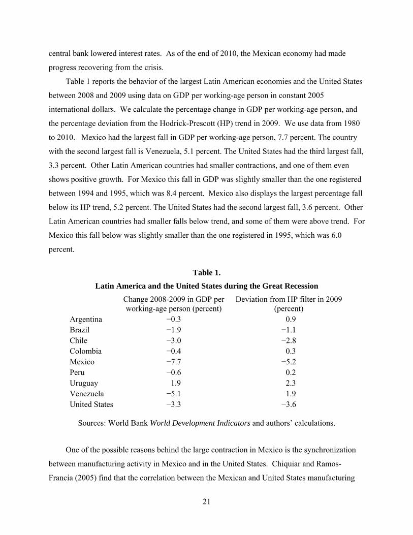
Table 1 reports the behavior of the largest Latin American economies and the United States
between 2008 and 2009 using data on GDP per working-age person in constant 2005
international dollars. We calculate the percentage change in GDP per working-age person, and
the percentage deviation from the Hodrick-Prescott (HP) trend in 2009. We use data from 1980
to 2010. Mexico had the largest fall in GDP per working-age person, 7.7 percent. The country
with the second largest fall is Venezuela, 5.1 percent. The United States had the third largest fall,
3.3 percent. Other Latin American countries had smaller contractions, and one of them even
shows positive growth. For Mexico this fall in GDP was slightly smaller than the one registered
between 1994 and 1995, which was 8.4 percent. Mexico also displays the largest percentage fall
below its HP trend, 5.2 percent. The United States had the second largest fall, 3.6 percent. Other
Latin American countries had smaller falls below trend, and some of them were above trend. For
Mexico this fall below was slightly smaller than the one registered in 1995, which was 6.0
percent.
Table 1.
Latin America and the United States during the Great Recession
Change 2008-2009 in GDP per working-age person (percent)
Deviation from HP filter in 2009 (percent)
Argentina −0.3 0.9 Brazil −1.9 −1.1 Chile −3.0 −2.8 Colombia −0.4 0.3 Mexico −7.7 −5.2 Peru −0.6 0.2 Uruguay 1.9 2.3 Venezuela −5.1 1.9 United States −3.3 −3.6
Sources: World Bank World Development Indicators and authors’ calculations.
One of the possible reasons behind the large contraction in Mexico is the synchronization
between manufacturing activity in Mexico and in the United States. Chiquiar and Ramos-
Francia (2005) find that the correlation between the Mexican and United States manufacturing
22
sectors increased after NAFTA. Looking at data on real value added by industry for the United
States, we see that manufacturing fell approximately 9 percent between 2008 and 2009. The
large fall in manufacturing in the United States can account for part of the contraction in
manufacturing, and therefore for part of the overall fall in GDP in Mexico.
Public policy in response to the crisis was in part countercyclical. This is an important
change compared to previous crises. In response to both the 1982 debt crisis and the 1994–1995
crisis, the government implemented fiscal austerity. From 2000 to 2008, the public sector deficit
fell from 1 percent of GDP to approximately zero.3 In 2009 the deficit rose to slightly more than
2 percent of GDP. The source of this increase in the deficit was a change in accounting rules.
According to Secretaría de Hacienda y Crédito Público (2010) in October 2008, the law that
rules the accounting of PEMEX, the national oil company, was modified so that certain
investments made by PEMEX, called PIDIREGAS (Proyectos de Inversión Diferida en el
Registro del Gasto, Investment Projects with Deferred Expenditure Registration), which were
not previously registered in the public deficit, would be recorded in it starting in 2009. If this
investment by PEMEX is excluded from the deficit, the deficit-GDP ratio is approximately zero
in 2009.
In terms of changes in taxation, the government implemented some procyclical measures in
2010. The government raised certain tax rates and created new taxes. On the other hand, for
2010, according to Secretaría de Hacienda y Crédito Público (2010), there would be a deficit-
GDP ratio of 2.7 percent considering investment made by PEMEX including PIDIREGAS, and
0.7 percent excluding it. The government said that the increase from approximately zero in 2009
to 0.7 percent in 2010 was part of the countercyclical measures in response to the current
international financial crisis.
Monetary policy during the Great Recession was countercyclical. The Banco de México
reduced its target interest rate starting in January 2009. The target fell from 8.25 percent at the
end of 2008 to 4.5 percent in July 2009. (See Banco de México 2009a, 2009b.) The interest rate
remained at that level during 2010.
3 The term “Public Sector” includes both the Federal Government and Institutions and Firms under Direct Budgetary Control (IFDBC). These IFDBC include PEMEX, the national oil company. The statistics related to the Public Sector exclude nonfinancial institutions and firms classified as under Indirect Budgetary Control (IFIBC). These statistics also exclude financial institutions controlled by the government, categorized as financial IFIBC, which are principally the development banks.
23
During 2010, the Mexican economy recovered partially from the crisis. Real GDP per
working-age person increased 3.2 percent. It still had not recovered its pre-crisis level, however.
A question of obvious importance is whether Mexico will grow at a higher rate than in the past
after the crisis is over, or if it will continue to display stagnation, conditional on a possible new
global recession.
4. The power of productivity
In this section, we analyze the performance of the Mexican economy during 1950–2010
using the one-sector neoclassical model. We argue that to understand the evolution of real GDP,
we need to understand the evolution of TFP. In the next section, we propose an extension of the
model to analyze the evolution of TFP in Mexico during 1950–2010.
The model has the aggregate production function
1t t t t t tC I Y A K L . (1)
Here, tK is the capital stock in period t, tL hours worked, tC aggregate consumption, and tI
aggregate investment. We subsume government consumption into tC and government
investment into tI . The parameter tA is TFP. The capital stock depreciates geometrically,
1t t t tK K K I . (2)
The stand-in household has the utility function
0
log 1 log tt t tt T
C hN L
. (3)
Here tN is the working-age population and h is the maximum amount of hours available for
work per person. The household’s budget constraint is
1 (1 )( )t t t t t t t t tC K K w L r K T . (4)
Here the wage rate tw and the rental rate tr are compatible with profit maximization by
competitive firms with the production function (1):
(1 )t t t tw A K L (5)
24
1 1t t t tr A K L . (6)
There is a tax on capital income with a tax rate t and tax revenues
( )t t t tT r K , (7)
which are redistributed in a lump-sum form to the household.
Suppose that both TFP and the working-age population grow at constant rates, 0t
tA A
and 0t
tN N . Then this economy has a unique balanced-growth path in which all the
quantities per working-age person grow by the factor 1/(1 )g , with the exception of market
hours per working-age person /t tL N , which are constant. It is this fact that motivates the
growth accounting employed by Kehoe and Prescott (2002, 2007). This growth accounting
rearranges terms in the production function to decompose the determinants of output into three
factors. The advantage of this decomposition is that each of the three factors leads us to examine
a different set of shocks and changes in policies when studying changes in output:
1
11t t tt
t t t
Y K LA
N Y N
. (8)
In this growth accounting, growth in human capital shows up as growth in TFP.
Fluctuations in factor utilization also show up as fluctuations in TFP, although this is probably
more important in studying business cycle moments, like the 1994–1995 financial crisis in
Mexico, than it is in studying growth over a decade or longer. The growth accounting in
equation (8), in contrast to that of Solow (1957) and Denison (1962), takes into account the
feature of the neoclassical growth model that, in a balanced-growth path, as technological growth
occurs, households save so as to keep the capital-output ratio constant. Researchers like De
Gregorio and Lee (2004) and Bosworth and Collins (2008), who use a growth accounting that
looks at increases in output per worker as a function of variables that include capital per worker,
typically find increases in TFP and increases in capital roughly equally important in accounting
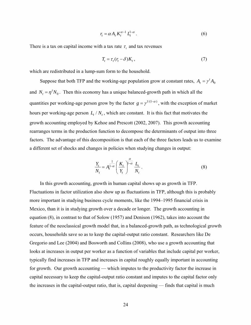
for growth. Our growth accounting — which imputes to the productivity factor the increase in
capital necessary to keep the capital-output ratio constant and imputes to the capital factor only
the increases in the capital-output ratio, that is, capital deepening — finds that capital is much
25
less important and that increases in productivity are typically the driving force of economic
growth.
Growth accounting for the United States
-1.0
0.0
1.0
2.0
1950 1960 1970 1980 1990 2000 2010
ind
ex
(1
95
0 =
10
0)
50
100
200
400
output
productivity
labor
capital
Figure 10.
Figure 10 presents this growth accounting for the United States over the period 1950–2010,
where we follow Bergoeing et al. (2002, 2007) in setting the capital share 0.30 . (All of the
data used in this growth accounting exercise and details on how we have processed these data are
available at www.umn.edu/~tkehoe.) Notice that theses data are close to those of a balanced-
growth path in that the capital factor /(1 )/t tK Y
and the labor factor /t tL N are close to
being constant, and growth in real GNP per working-age person /t tY N is driven by growth in
the productivity factor 1/(1 )tA .
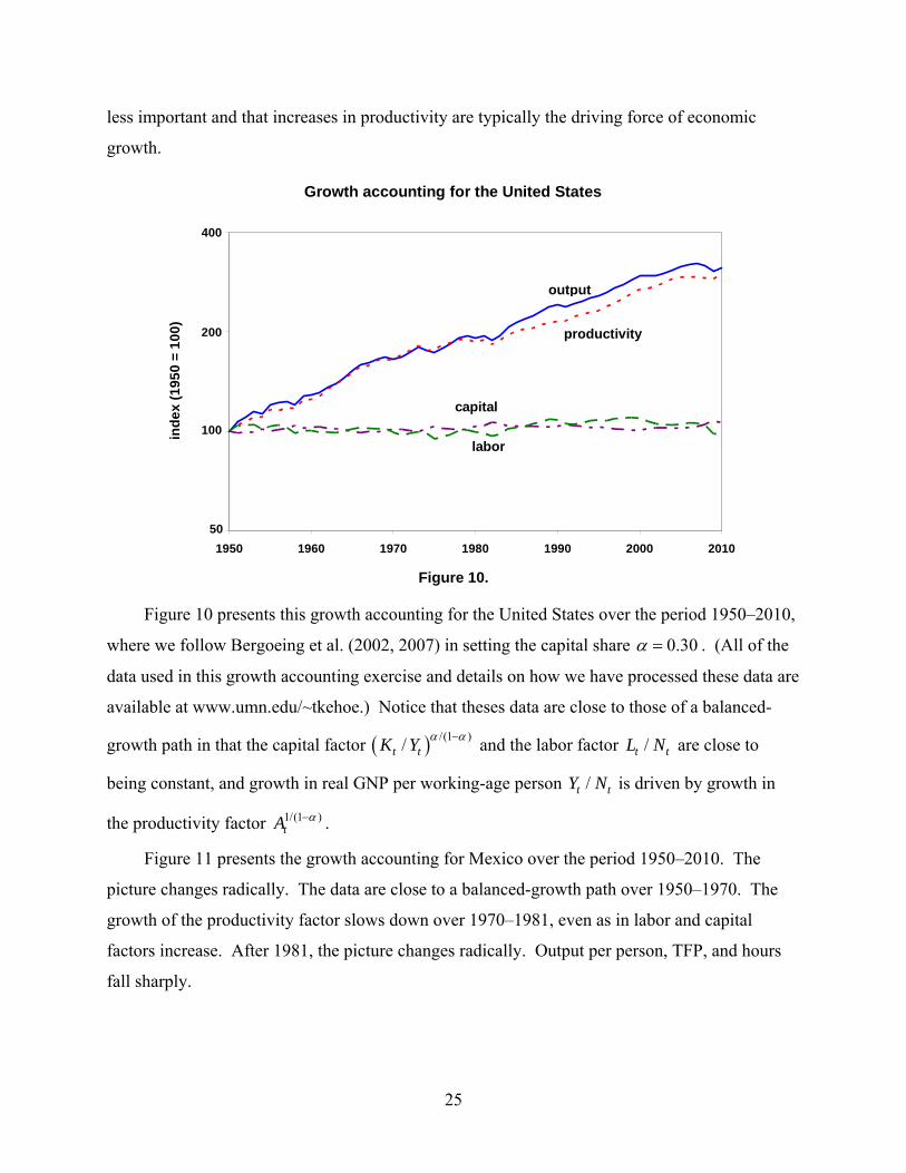
Figure 11 presents the growth accounting for Mexico over the period 1950–2010. The
picture changes radically. The data are close to a balanced-growth path over 1950–1970. The
growth of the productivity factor slows down over 1970–1981, even as in labor and capital
factors increase. After 1981, the picture changes radically. Output per person, TFP, and hours
fall sharply.

26
Growth accounting for Mexico
-1.0
0.0
1.0
2.0
1950 1960 1970 1980 1990 2000 2010
ind
ex
(1
95
0 =
10
0)
50
100
200
400
output
productivity
labor
capital
Figure 11.
The calibration of the parameters of the model and the computation of its equilibrium
follow Bergoeing et al. (2002, 2007). To estimate the consumption weight , we use the
intratemporal first-order condition from the household’s utility maximization problem,
1 1
t
t t t t t
C
hN L A K L
. (9)
We set h equal to 100 hours per week and average over 1950–1960 data to estimate 0.257 .
To calibrate the tax rate, we use the intertemporal first-order condition from the household’s
utility maximization problem, assuming that t is constant,
11 1
1
1 t t
t t t t
C C
A K H C
. (10)
We set 0.980 and average over 1950–1960 data to estimate 0.509 . We have included a
tax on capital in the model because Bergoeing et al. (2002, 2007) argue that fiscal reforms in
Mexico in the late 1980s play a major role in determining capital accumulation there. We will
also run a numerical experiment where we set 0.509t for 1950,1951,...,1987t but have t
unexpectedly change to 0.254 in 1988 and afterwards.
27
Ideally, we would calibrate the parameters and to data from before 1950 so that we
could avoid fitting consumption-savings and consumption-leisure decisions in the model to the
period in which we are interested. Unfortunately, we do not have enough data from before 1950
to do this. We calibrate the model to 1950–1960 data, and, assuming that the capital-output ratio
in 1950 is equal to its average over 1950–1960, we calculate an initial capital stock 1950K . Since
we calibrate the parameters of the model to 1950–1960 data, we should not be surprised to see
the model fit the data well for this period. The test of the model is how well it does for 1960–
2010.
Given the calibrated model, we can perform numerical experiments. In the first
experiment, we start the model in 0 1950T with the initial value of the capital stock 1950K . We
set the values for the TFP series 1950 1951, ,...A A , equal to the observed values over the period
1950–2010 and let tA grow at the rate of 1.40 percent per year after that, which corresponds to a
balanced-growth rate in output per working-age person of 2 percent per year,
1 0.71.0140 1.02 1.02 . We also set the values for the working-age population
1950 1951, ,...N N equal to the observed values over the period 1950–2010 and let tN grow at the
rate of 1.69 percent per year after that, where 1.69 percent per year was the observed growth rate
of the working-age population in 2010. All of the other variables are computed endogenously.
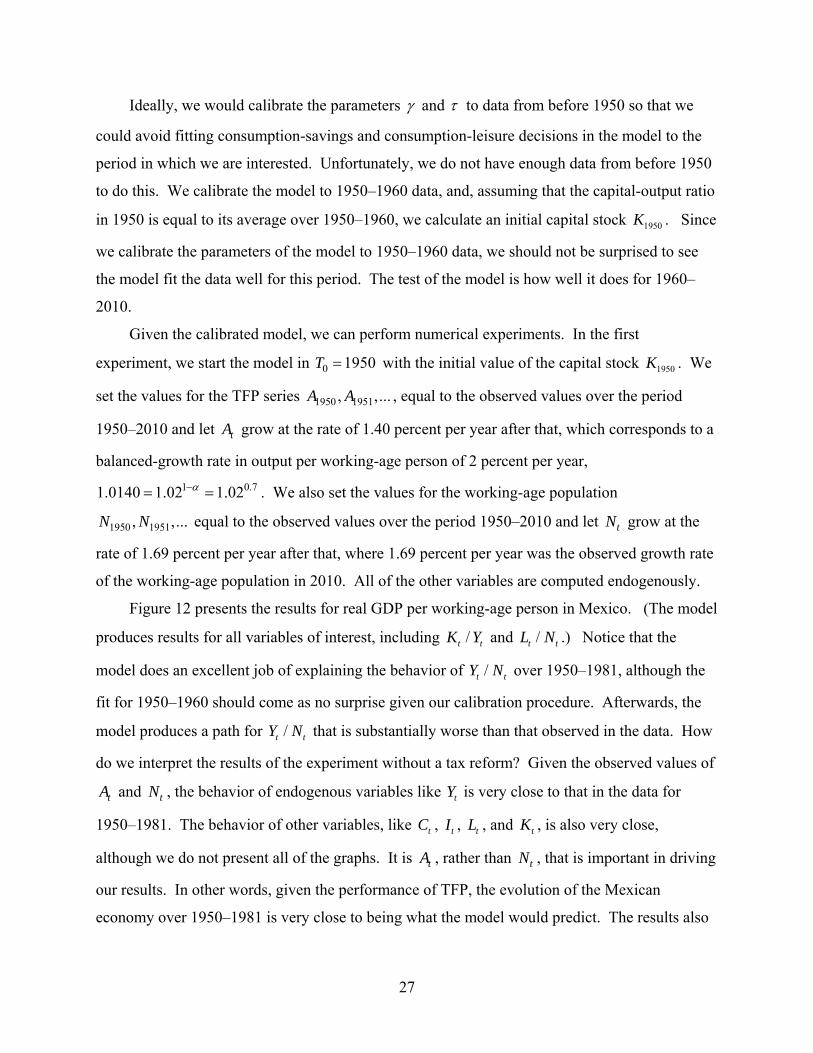
Figure 12 presents the results for real GDP per working-age person in Mexico. (The model
produces results for all variables of interest, including /t tK Y and /t tL N .) Notice that the
model does an excellent job of explaining the behavior of /t tY N over 1950–1981, although the
fit for 1950–1960 should come as no surprise given our calibration procedure. Afterwards, the
model produces a path for /t tY N that is substantially worse than that observed in the data. How
do we interpret the results of the experiment without a tax reform? Given the observed values of
tA and tN , the behavior of endogenous variables like tY is very close to that in the data for
1950–1981. The behavior of other variables, like tC , tI , tL , and tK , is also very close,
although we do not present all of the graphs. It is tA , rather than tN , that is important in driving
our results. In other words, given the performance of TFP, the evolution of the Mexican
economy over 1950–1981 is very close to being what the model would predict. The results also
28
indicate that, had nothing else besides observed productivity and population changed after 1982,
the Mexican economy would have done far worse than it actually did.
Real GDP per working-age person in Mexico
50
100
150
200
250
300
350
1950 1960 1970 1980 1990 2000 2010
ind
ex
(1
95
0 =
10
0) model
data
model withouttax reform
Figure 12.
Bergoeing et al. (2002, 2007) argue that in the late 1980s a series of fiscal reforms in
Mexico changed the incentives to accumulate capital. To capture the impact of these reforms we
run another numerical experiment, identical to the first except that in 1988 we change t from
0.509 to 0.254 and leave it at this level. We model this change as unexpected by households.
The model now does much better in tracking the performance of the Mexican economy over
1982–2010. Our conclusion is that, if we take into account a major change in incentives to
accumulate capital in the 1980s and if we can understand the evolution of TFP in Mexico, we
understand most of the evolution of the Mexican macroeconomy over 1950–2010.
It is worth noting that this model can be modified to include foreign trade and investment,
as in Kehoe and Ruhl (2009). This modification, especially the modeling of the inflow of
foreign investment in the early 1990s and its sudden stop in 1995–1996, can improve the
performance of the model even further.
Many other authors, going back to the late 1950s, have realized that understanding TFP
growth is essential for understanding economic growth. Of particular relevance for the
theoretical framework that we sketch out in the next section are Lewis (2004) and Parente and
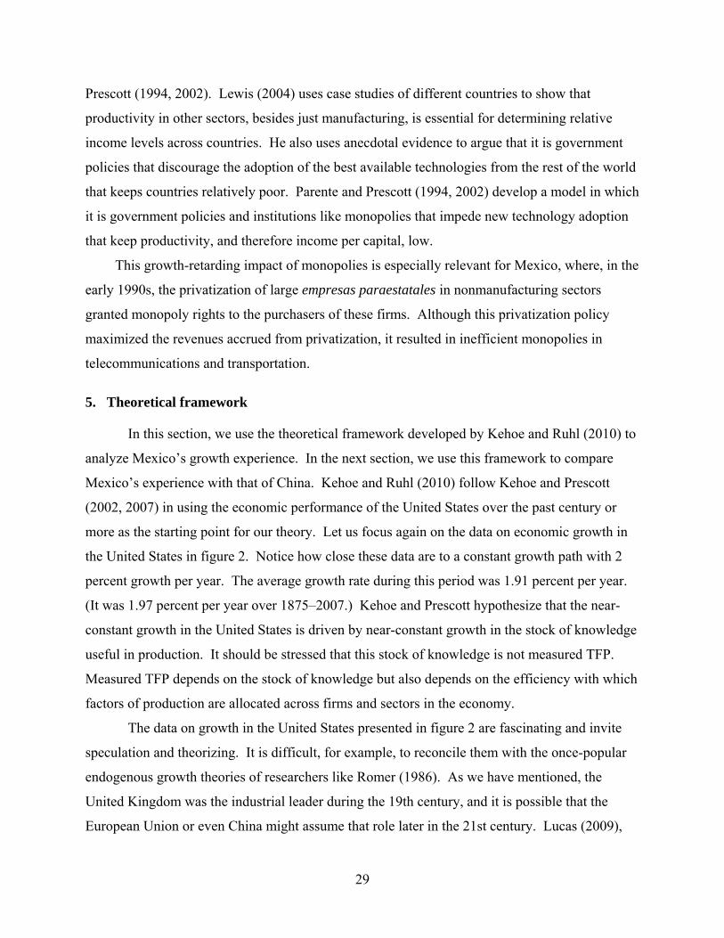
29
Prescott (1994, 2002). Lewis (2004) uses case studies of different countries to show that
productivity in other sectors, besides just manufacturing, is essential for determining relative
income levels across countries. He also uses anecdotal evidence to argue that it is government
policies that discourage the adoption of the best available technologies from the rest of the world
that keeps countries relatively poor. Parente and Prescott (1994, 2002) develop a model in which
it is government policies and institutions like monopolies that impede new technology adoption
that keep productivity, and therefore income per capital, low.
This growth-retarding impact of monopolies is especially relevant for Mexico, where, in the
early 1990s, the privatization of large empresas paraestatales in nonmanufacturing sectors
granted monopoly rights to the purchasers of these firms. Although this privatization policy
maximized the revenues accrued from privatization, it resulted in inefficient monopolies in
telecommunications and transportation.
5. Theoretical framework
In this section, we use the theoretical framework developed by Kehoe and Ruhl (2010) to
analyze Mexico’s growth experience. In the next section, we use this framework to compare
Mexico’s experience with that of China. Kehoe and Ruhl (2010) follow Kehoe and Prescott
(2002, 2007) in using the economic performance of the United States over the past century or
more as the starting point for our theory. Let us focus again on the data on economic growth in
the United States in figure 2. Notice how close these data are to a constant growth path with 2
percent growth per year. The average growth rate during this period was 1.91 percent per year.
(It was 1.97 percent per year over 1875–2007.) Kehoe and Prescott hypothesize that the near-
constant growth in the United States is driven by near-constant growth in the stock of knowledge
useful in production. It should be stressed that this stock of knowledge is not measured TFP.
Measured TFP depends on the stock of knowledge but also depends on the efficiency with which
factors of production are allocated across firms and sectors in the economy.
The data on growth in the United States presented in figure 2 are fascinating and invite
speculation and theorizing. It is difficult, for example, to reconcile them with the once-popular
endogenous growth theories of researchers like Romer (1986). As we have mentioned, the
United Kingdom was the industrial leader during the 19th century, and it is possible that the
European Union or even China might assume that role later in the 21st century. Lucas (2009),
30
for example, develops a model of the development of new ideas that he parameterizes to yield a
growth rate of 2 percent per year. This model might be useful in thinking about how this long-
run growth rate might change. It is possible, for example, that technological progress may be
slowly accelerating: as we have mentioned, according to Maddison (1995), in the United
Kingdom the average growth of real GDP per capita 1820–1900 was 1.2 percent per year. While
all of this is interesting, it is mostly relevant for countries at the technological frontier, countries
like the United States, Canada, and Japan and countries in Western Europe where what Lewis
(2004) calls “best practice” is developed. It is largely irrelevant to our question involving growth
in Mexico, a country that is behind the industrial leader and simply needs to adapt best practice
from elsewhere.
Kehoe and Ruhl (2010) hypothesize that the stock of knowledge, which has increased very
smoothly over the past century or more, can be adopted, perhaps at some cost by countries that
are behind the industrial leader. This would give rise to trend growth of close to 2 percent per
year, at least after capital and labor have had time to adjust. In this framework, changes in
policies — such as the development of railroads during the Porfiriato and of the policies to
promote urbanization, industrialization, and education during the recovery from the Revolución
and the Great Depression and the import substitution period that followed — affect only the
levels of a balanced-growth path. Long-run growth remains at 2 percent per year. The absolute
level that a specific country is at compared to the industrial leader depends on its institutions and
economic policies. Changes in these institutions and economic policies can cause depressions or
booms. Eventually, however, if institutions and policies stabilize, and after capital and labor
have adjusted, the country returns to trend growth.
How do we interpret the economic history of Mexico in terms of this theory? Changes in
economic policies during the Porfiriato and the recovery from the Revolución and the Great
Depression led to catch-up growth. Policy mistakes made during the end of the import
substitution period 1970–1981 led to the crises that followed. After 1995, we interpret Mexico
as being in the balanced-growth path that its policies and institutions warrant.
What are the factors that impede Mexico from continuing catch-up growth and reaching
levels of income like that in its neighbors and trade partners, Canada and the United States? A
number of researchers have addressed this question and conclude that Mexico’s slow growth,
despite its reforms over 1985–1995, is a consequence of its inefficient financial system and lack
31
of contract enforcement. Bergoeing et al. (2002, 2007) compare the growth trajectories of Chile
and Mexico following the financial crises they both suffered in the 1980s; Chile recovered
rapidly while Mexico stagnated. They conclude that the crucial differences between policies in
Mexico and Chile are those related to the banking system and to bankruptcy proceedings.
Krueger and Tornell (1999) and Tornell et al. (2003) also find that the lack of credit, particularly
in the nontradable goods sector, was responsible for the poor growth in Mexico. The data in
figure 4 show the very low levels of credit that the Mexican financial sector provides the private
sector. In 1950–1981 the economy was able to grow in spite of the inefficient financial sector
because the government did much of the investment. One indicator of the problems in contract
enforcement in Mexico, besides anecdotal evidence, is precisely this low level of credit. Another
indicator is the data from the World Bank’s Doing Business on the costs of recovering damages
from a broken contract presented in table 2. Another barrier to growth in Mexico is the rigid
labor market. Kambourov (2009), for example, presents evidence for this rigidity and argues
that it prevented Mexico from benefiting as much from opening to trade as Chile did. The last
column in table 2 presents data collected by Heckman and Pagés (2000) on the costs of job
security regulation, another measure of labor market rigidity.4
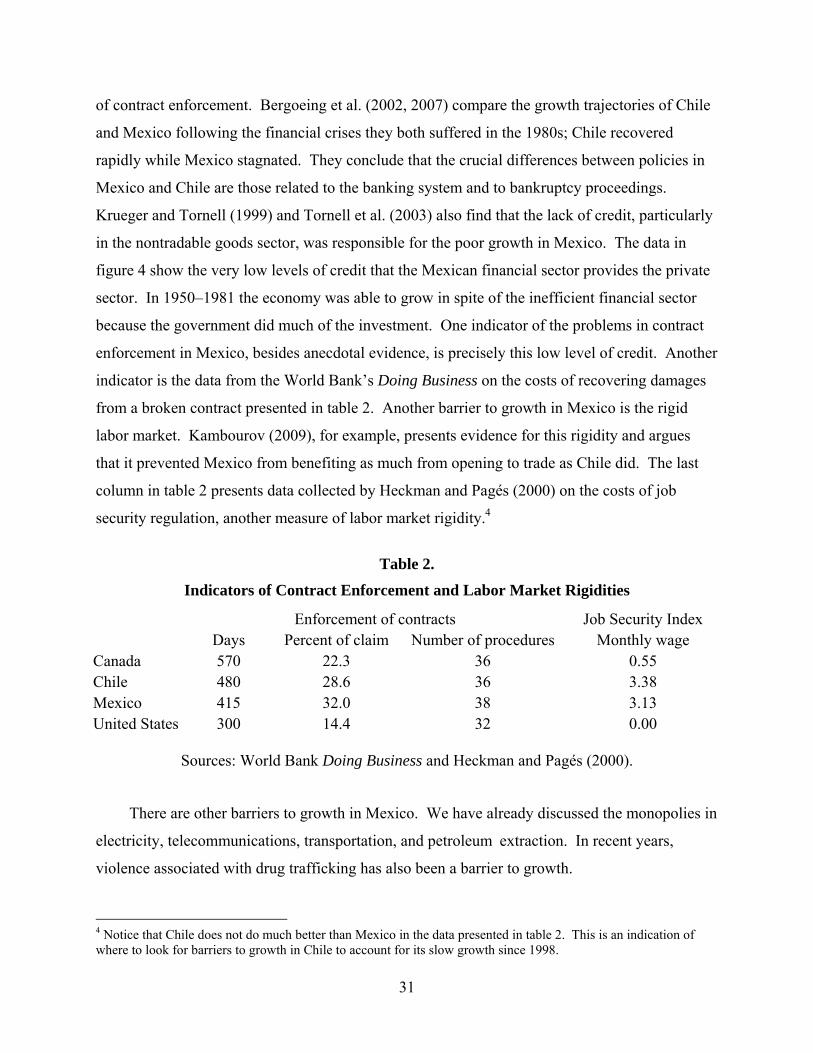
Table 2.
Indicators of Contract Enforcement and Labor Market Rigidities
Enforcement of contracts Job Security Index Days Percent of claim Number of procedures Monthly wage Canada 570 22.3 36 0.55 Chile 480 28.6 36 3.38 Mexico 415 32.0 38 3.13 United States 300 14.4 32 0.00
Sources: World Bank Doing Business and Heckman and Pagés (2000).
There are other barriers to growth in Mexico. We have already discussed the monopolies in
electricity, telecommunications, transportation, and petroleum extraction. In recent years,
violence associated with drug trafficking has also been a barrier to growth.
4 Notice that Chile does not do much better than Mexico in the data presented in table 2. This is an indication of where to look for barriers to growth in Chile to account for its slow growth since 1998.

32
6. Mexico versus China
China is another large, less-developed country that has opened itself to foreign trade and
investment, and to which Mexico is often compared. Growth in recent years in China has been
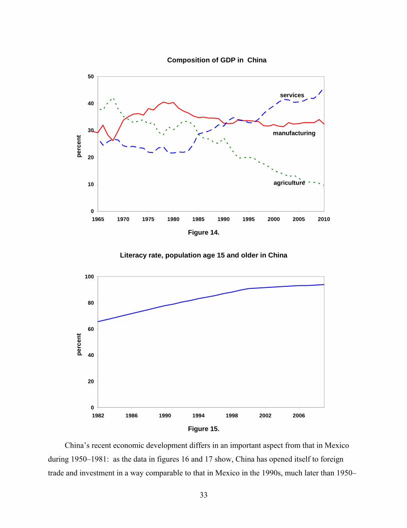
spectacular. As the data in figures 13, 14, and 15 show, the same forces that drove rapid growth
in Mexico during 1950–1981 have been at play more recently in China: urbanization,
industrialization, and education. Notice that in figure 13 China is still substantially behind
Mexico in terms of urbanization and that in figure 14 it is still substantially behind in terms of
industrialization.5 It is only in the data on education in figure 15 where China is ahead of
Mexico.
Urban population in China
10
20
30
40
50
1960 1965 1970 1975 1980 1985 1990 1995 2000 2005
pe
rce
nt
Figure 13.
5 The data in figure 13 are not strictly comparable to those in figure 7, but they are close. The definition of urban population has changed a number of times in the Chinese census, but up until 1982 the urban population was that living in cities and towns, where towns were defined as either settlements with more than 3,000 inhabitants of whom more than 70 percent were registered as nonagricultural or settlements with a population ranging from 2,500 to 3,000 inhabitants of whom more than 85 percent were registered as nonagricultural.
33
Composition of GDP in China
0
10
20
30
40
50
1965 1970 1975 1980 1985 1990 1995 2000 2005 2010
pe
rce
nt
agriculture
services
manufacturing
Figure 14.
Literacy rate, population age 15 and older in China
0
20
40
60
80
100
1982 1986 1990 1994 1998 2002 2006
pe
rce
nt
Figure 15.
China’s recent economic development differs in an important aspect from that in Mexico
during 1950–1981: as the data in figures 16 and 17 show, China has opened itself to foreign
trade and investment in a way comparable to that in Mexico in the 1990s, much later than 1950–
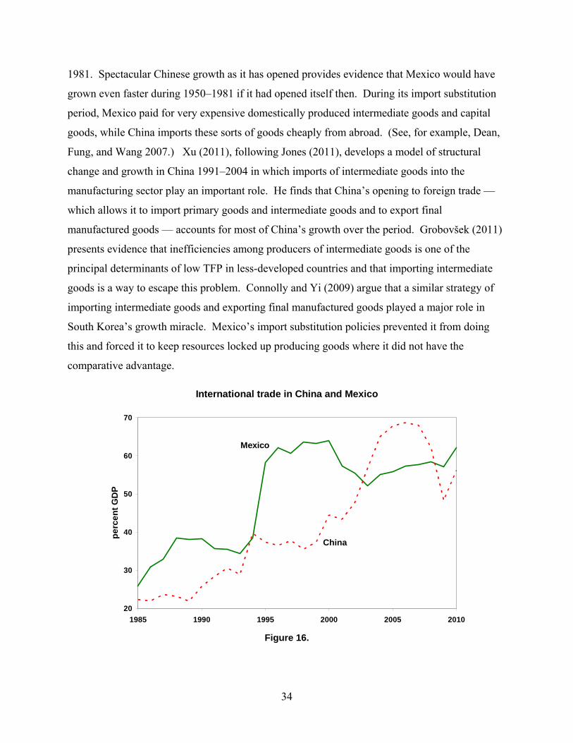
34
1981. Spectacular Chinese growth as it has opened provides evidence that Mexico would have
grown even faster during 1950–1981 if it had opened itself then. During its import substitution
period, Mexico paid for very expensive domestically produced intermediate goods and capital
goods, while China imports these sorts of goods cheaply from abroad. (See, for example, Dean,
Fung, and Wang 2007.) Xu (2011), following Jones (2011), develops a model of structural
change and growth in China 1991–2004 in which imports of intermediate goods into the
manufacturing sector play an important role. He finds that China’s opening to foreign trade —
which allows it to import primary goods and intermediate goods and to export final
manufactured goods — accounts for most of China’s growth over the period. Grobovšek (2011)
presents evidence that inefficiencies among producers of intermediate goods is one of the
principal determinants of low TFP in less-developed countries and that importing intermediate
goods is a way to escape this problem. Connolly and Yi (2009) argue that a similar strategy of
importing intermediate goods and exporting final manufactured goods played a major role in
South Korea’s growth miracle. Mexico’s import substitution policies prevented it from doing
this and forced it to keep resources locked up producing goods where it did not have the
comparative advantage.
International trade in China and Mexico
20
30
40
50
60
70
1985 1990 1995 2000 2005 2010
pe
rce
nt
GD
P
Mexico
China
Figure 16.

35
Foreign direct investment in China and Mexico
0
2
4
6
1985 1990 1995 2000 2005 2010
pe
rce
nt
GD
P
Mexico
China
Figure 17.
Identifying an inefficient financial system and lack of contract enforcement as the factors
that retard Mexican growth generates a puzzle because China also suffers from these problems.
China has been able to grow with a poorly functioning financial and legal system, despite the
lack of significant reforms to these systems (Rawski 1994, Allen, Qian, and Qian 2005).
Studying the Chinese experience, Guariglia and Poncet (2008) go so far as to question whether
an efficient financial system is necessary for growth.
What factors have driven growth in China, and are these factors present in Mexico? Studies
of China’s output growth, such as Brandt and Zhu (2009) and Hsieh and Klenow (2009),
conclude that productivity growth arising from the reallocation of resources across firms is key.
It would be tempting to hypothesize that the mechanisms that generated productivity growth in
manufacturing in China were not present in Mexico, but López-Córdova (2003) finds that trade
and foreign investment reforms resulted in large increases in productivity in the manufacturing
sector in Mexico, especially in those sectors most exposed to foreign trade. This suggests that
the problem in Mexico is not a lack of productivity growth in manufacturing, but in the rest of
the economy.
Our solution to the puzzle of why China has grown rapidly and why Mexico has not is
that China is still at a lower level of development than Mexico and the barriers to growth in
36
Mexico — especially the inefficient financial system and lack of contract enforcement — have
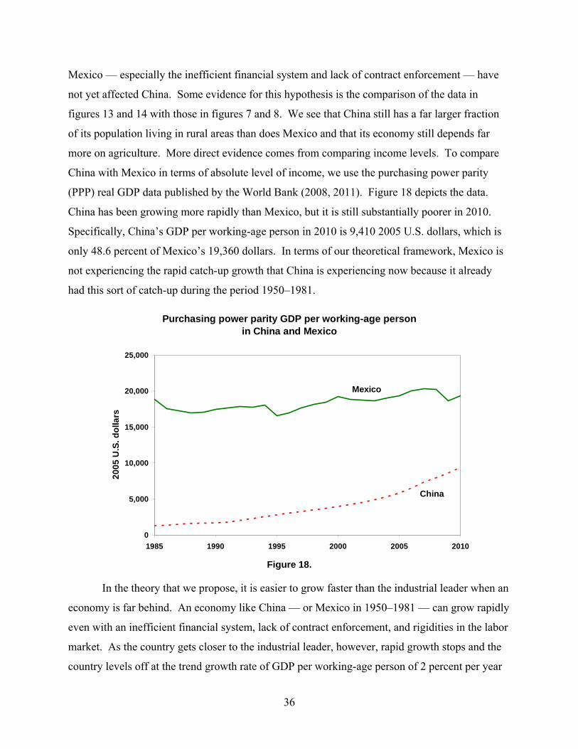
not yet affected China. Some evidence for this hypothesis is the comparison of the data in
figures 13 and 14 with those in figures 7 and 8. We see that China still has a far larger fraction
of its population living in rural areas than does Mexico and that its economy still depends far
more on agriculture. More direct evidence comes from comparing income levels. To compare
China with Mexico in terms of absolute level of income, we use the purchasing power parity
(PPP) real GDP data published by the World Bank (2008, 2011). Figure 18 depicts the data.
China has been growing more rapidly than Mexico, but it is still substantially poorer in 2010.
Specifically, China’s GDP per working-age person in 2010 is 9,410 2005 U.S. dollars, which is
only 48.6 percent of Mexico’s 19,360 dollars. In terms of our theoretical framework, Mexico is
not experiencing the rapid catch-up growth that China is experiencing now because it already
had this sort of catch-up during the period 1950–1981.
Purchasing power parity GDP per working-age person in China and Mexico
0
5,000
10,000
15,000
20,000
25,000
1985 1990 1995 2000 2005 2010
20
05
U.S
. do
llars
Mexico
China
Figure 18.
In the theory that we propose, it is easier to grow faster than the industrial leader when an
economy is far behind. An economy like China — or Mexico in 1950–1981 — can grow rapidly
even with an inefficient financial system, lack of contract enforcement, and rigidities in the labor
market. As the country gets closer to the industrial leader, however, rapid growth stops and the
country levels off at the trend growth rate of GDP per working-age person of 2 percent per year
37
or a little less. This seems to have occurred in Western Europe in the early 1970s, in Japan in the
early 1990s, and in Chile in the late 1990s, to mention a few cases. How far short of the
industrial leader the country levels off depends on its institutions and economic policies. Chile,
for example, after spectacular growth following its great depression in the early 1980s, has had a
level of real GDP per working-age person and a growth rate similar to those in Mexico since
about 1998. Unless China continues to reform, we can expect economic growth there to slow
down sharply at some point. It is an open question whether or not this slowdown will occur
when China is still behind Mexico in terms of real GDP per working-age person.6
7. Outlook for the future
Many open questions remain to be resolved for our theory to be useful in accounting for the
economic development of countries like Mexico and China: In general, is openness to trade and
foreign investment necessary for rapid growth when a country is very far behind the industrial
leader? India’s recent experience along with Mexico’s experience 1950–1981 suggest not.
Specific questions about the experience of Mexico remain to be resolved as well: Why was the
period of rapid growth, 1995–2000, following the enactment of NAFTA so short? Or, put
another way, why was the recovery following the 1982–1995 great depression so modest? It
may be that Mexico’s slower growth since 2000 is the product of the contraction of the U.S.
manufacturing sector and of competition with China. Perhaps most importantly, what sorts of
reforms does Mexico need to enact to resume rapid catch-up growth? We hypothesize that these
are reforms that eliminate the barriers to growth of an inefficient financial system, lack of
contract enforcement, and rigidities in the labor market. In terms of more specific reforms,
promoting competition in nonmanufacturing sectors like electricity, telecommunications, and
transportation would spur productivity growth. So would allowing private investment in
petroleum extraction. Reducing violence related to drug trafficking would also have a positive
impact.
6 Our theory suggests that it may be more fruitful to compare Mexico to economies at a similar level of economic development. Brazil is a frequently cited example. It is a country that has about 80 percent of the real GDP per working-age person of Mexico in 2010 but that has experienced higher rates of growth than Mexico since 2000. Over the period 1995–2007, however, the growth rate of GDP per working age person in Brazil has been 1.1 percent per year, less than Mexico’s 1.7 percent per year. Despite high growth in 2009 and 2010, it has yet to be seen whether Brazil is performing significantly better than Mexico.

38
Our analysis also points to directions for future research. We could expand the one-sector
growth model discussed in sections 4 and 5 to a model like those in Buera and Kaboski
(forthcoming) and Echevarria (1997, 2008) with primary, manufacturing, and service sectors.
The analysis in Xu (2011) indicates that it would also be useful to disaggregate manufacturing
into intermediate goods and final goods. With such a model, we could quantify more precisely
the costs and benefits of import substitution during the period of Mexico’s fast growth 1950–
1981. With such a model, we could also extend the theory of barriers to growth and transitions
to higher balanced-growth paths sketched out in section 5 to incorporate the stages of growth
studied by Rostow (1960).
39
References
Allen, F., J. Qian, and M. Qian (2005), “Law, finance, and economic growth in China,” Journal of Financial Economics 77: 57–116.
Aspe, P. (1993), El Camino Mexicano de la Transformación Económica, 2nd ed., Mexico, Fondo de Cultura Económica.
Banco de México (2009a), Anuncio de Política Monetaria, 26 January 2009, Banco de México.
Banco de México (2009b), Anuncio de Política Monetaria, 17 July 2009, Banco de México.
Bergoeing, R., P.J. Kehoe, T.J. Kehoe, and R. Soto (2002), “A decade lost and found: Mexico and Chile in the 1980s,” Review of Economic Dynamics 5: 166–205.
Bergoeing, R., P.J. Kehoe, T.J. Kehoe, and R. Soto (2007), “A decade lost and found: Mexico and Chile in the 1980s,” in T.J. Kehoe and E. C. Prescott, eds., Great Depressions of the Twentieth Century, 217–56, Minneapolis, MN, Federal Reserve Bank of Minneapolis.
Bosworth, B., and S.M. Collins (2008), “Accounting for growth: Comparing China and India,” Journal of Economic Perspectives 22: 45–66.
Brandt, L., and X. Zhu ( 2009), “Accounting for China’s growth,” IZA Discussion Paper 4764, Institute for the Study of Labor (IZA).
Buera, F.J., and J.P. Kaboski (forthcoming), “Scale and the origins of structural change,” Journal of Economic Theory.
Cárdenas, E. (1996), La Política Económica en México, 1950-1994, Mexico, El Colegio de México, Fideicomiso Historia de las Américas, Fondo de Cultura Económica.
Chiquiar, D., and M. Ramos-Francia (2005), “Trade and business-cycle synchronization: Evidence from Mexican and U.S. manufacturing industries,” North American Journal of Economics and Finance 16: 187–216.
Cole, H. L., and T. J. Kehoe (1996), “A self-fulfilling model of Mexico’s 1994–95 debt crisis,” Journal of International Economics 41: 309–30.
Connolly, M., and K-M. Yi (2009), “How much of South Korea’s growth miracle can be explained by trade policy?” Working Paper 09-19, Federal Reserve Bank of Philadelphia.
De Gregorio, J., and J-W. Lee (2004), “Growth and adjustment in East Asia and Latin America,” Economía 5: 69–134.
Dean, J., K.C. Fung, and Z. Wang (2007), “Measuring the vertical specialization in Chinese Trade,” Working Paper 2007-01-A, U.S. International Trade Commission, Office of Economics.
Denison, E.F. (1962), “The sources of economic growth in the United States and the alternatives before us,” Supplementary Paper No. 13, New York, Committee for Economic Development.
Echevarria, E.C. (1997), “Changes in sectoral composition associated with economic growth,” International Economic Review 38: 431–52.
Echevarria, E.C. (2008), “International trade and the sectoral composition of production,” Review of Economic Dynamics 11: 192–206.
40
Grobovšek, J. (2011), “Development accounting with intermediate goods,” Universitat Autònoma de Barcelona.
Guariglia, A., and S. Poncet (2008), “Could financial distortions be no impediment to growth after all? Evidence from China,” Journal of Comparative Economics 36: 633–57.
Haber, S. (2009), “Why banks do not lend: The Mexican financial system,” in S. Levy and M. Walton, eds., No Growth without Equity? Inequality, Interests and Competition in Mexico, 283–317, New York, NY, Palgrave Macmillan and the World Bank.
Heckman, J., and C. Pagés (2000), “The cost of job security regulation: Evidence from Latin American labor markets,” Research Department Working Paper 430, Inter-American Development Bank.
Hsieh, C-T., and P.J. Klenow (2009), “Misallocation and manufacturing TFP in China and India,” Quarterly Journal of Economics 124: 1403–48.
Instituto Nacional de Estadística y Geografía (INEGI) (2009), Estadisticas Historicas de Mexico, Aguacalientes, Mexico, Instituto Nacional de Estadística y Geografía.
International Monetary Fund, International Financial Statistics Database, accessed 28 November 2011, http://www.imf.org/external/data.htm.
Jones, C.I. (2011), “Intermediate goods and weak links in the theory of economic development,” American Economic Journal: Macroeconomics 3: 1–28.
Kambourov, G. (2009), “Labour market regulations and the sectoral reallocation of workers: The case of trade reforms,” Review of Economic Studies 76: 1321–58.
Kehoe, T.J. (1995a), “A review of Mexico’s trade policy from 1982 to 1994,” World Economy 18: 135–51.
Kehoe, T.J. (1995b), “What happened in Mexico in 1994–95?” in P. J. Kehoe and T. J. Kehoe, eds., Modeling North American Economic Integration, 131–47, Dordrecht, Netherlands, Kluwer Academic Publishers.
Kehoe, T.J., and E.C. Prescott (2002), “Great depressions of the 20th century,” Review of Economic Dynamics 5: 1–18.
Kehoe, T.J., and E.C. Prescott, eds. (2007), Great Depressions of the Twentieth Century, Minneapolis, MN, Federal Reserve Bank of Minneapolis.
Kehoe, T.J., and K.J. Ruhl (2009), “Sudden stops, sectoral reallocations, and the real exchange rate,” Journal of Development Economics 89: 235–49.
Kehoe, T.J., and K.J. Ruhl (2010), “Why have economic reforms in Mexico not generated growth?,” Journal of Economic Literature 48: 1005–27.
Kehoe, T.J., and K.J. Ruhl (2011), “Does openness generate growth? Reconciling the experiences of Mexico and China,” VoxEU, 19 November 2011, http://voxeu.org/index.php?q=node/7301.
Krueger, A., and A. Tornell (1999), “The role of bank restructuring in recovering from crises: Mexico 1995–1998,” Working Paper 7042, Cambridge, MA, NBER.
41
Lewis, W.W. (2004), The Power of Productivity: Wealth, Poverty, and the Threat to Global Stability, Chicago, University of Chicago Press.
López-Córdova, E. (2003), “NAFTA and manufacturing productivity in Mexico,” Economía 4: 55–98.
Lucas, R.E. (2009), “Ideas and Growth,” Economica 76: 1–19.
Maddison, A. (1995), Monitoring the World Economy: 1820–1992, Washington, DC, Organisation for Economic Co-operation and Development.
Maddison, A. (2010), “Historical Statistics of the World Economy: 1-2008 AD” (Excel file), accessed 26 November 2011, http://www.ggdc.net/MADDISON/Historical_Statistics/horizontal-file_02-2010.xls.
Meza, F. (2008), “Financial crisis, fiscal policy and the 1995 GDP contraction in Mexico,” Journal of Money, Credit and Banking 40: 1239–61.
Meza, F., and E. Quintin (2007), “Factor utilization and the real impact of financial crises,” B.E. Journal of Macroeconomics 7: article 33.
Parente, S.L., and E.C. Prescott (1994), “Barriers to technology adoption and development,” Journal of Political Economy 102: 298–321.
Parente, S.L., and E.C. Prescott (2002), Barriers to Riches, Cambridge, MA, MIT Press.
Ramos-Francia, M., and A. Torres-García (2005), “Reducing inflation through inflation targeting: The Mexican experience,” Working Paper 2005-01, Banco de México.
Rawski, T.G. (1994), “Chinese industrial reform: Accomplishments, prospects, and implications,” American Economic Review 84: 271–75.
Romer, P.M. (1986), “Increasing returns and long-run growth,” Journal of Political Economy 94: 1002-1037.
Rostow, W.W. (1960), The Stages of Economic Growth: A Non-Communist Manifesto, Cambridge, Cambridge University Press.
Secretaría de Hacienda y Crédito Público (2010), Criterios Generales de Política Económica 2011, Mexico, Secretaría de Hacienda y Crédito Público.
Solís Manjarrez, L. (2000), La realidad económica mexicana: Retrovisión y perspectivas, 3rd ed., México, El Colegio Nacional, Fondo de Cultura Económica.
Solow, R.M. (1957), “Technical change and the aggregate production function,” Review of Economics and Statistics 39: 312–20.
Tornell, A., F. Westermann, and L. Martinez (2003), “Liberalization, growth, and financial crises: Lessons from Mexico and the developing world,” Brookings Papers on Economic Activity 2003: 1–88.
World Bank (2008), “Global purchasing power parities and real expenditures,” in 2005 International Comparison Program, Washington, DC, World Bank.
World Bank, World Development Indicators Database, accessed 1 December 2011, http://data.worldbank.org/.

42
Xu, N. (2011), “Reallocation, globalization, and economic growth in China,” University of Minnesota.