Carlo R. Laing and S. Coombes- The importance of different timings of excitatory and inhibitory pathways in neural field models

8/3/2019 Carlo R. Laing and S. Coombes- The importance of different timings of excitatory and inhibitory pathways in neura…

http://slidepdf.com/reader/full/carlo-r-laing-and-s-coombes-the-importance-of-different-timings-of-excitatory 1/38

The importance of different timings of excitatory and

inhibitory pathways in neural field models

Carlo R. Laing∗

Institute of Information and Mathematical Sciences, Massey University,

Private Bag 102-904 North Shore Mail Centre, Auckland, New Zealand

and

S. Coombes†

Department of Mathematical Sciences,

University of Nottingham, Nottingham, NG7 2RD, UK.

December 23, 2005

Running title: “Different timings in neural field models”

Corresponding author:

Carlo R. Laing,

Institute of Information and Mathematical Sciences,

Massey University, Private Bag 102-904 North Shore Mail Centre,

Auckland, New Zealand

ph: +64-9-4140800 extn 41038

fax: +64-9-441-8136

email: [email protected]

∗email: [email protected]†email: [email protected]

1



The importance of different timings of excitatory and inhibitorypathways in neural field models

Abstract

In this paper we consider a neural field model comprised of two distinct popula-

tions of neurons, excitatory and inhibitory, for which both the velocities of action po-

tential propagation and the time courses of synaptic processing are different. Using

recently-developed techniques we construct the Evans function characterising the sta-

bility of both stationary and travelling wave solutions, under the assumption that the

firing rate function is the Heaviside step. We find that these differences in timing for

the two populations can cause instabilities of these solutions, leading to, for example,

stationary breathers. We also analyse “anti-pulses,” a novel type of pattern for which

all but a small interval of the domain (in moving coordinates) is active. These results

extend previous work on neural fields with space-dependent delays, and demonstrate

the importance of considering the effects of the different time-courses of excitatory and

inhibitory neural activity.

2



The importance of different timings of excitatory and inhibitorypathways in neural field models

1 Introduction

Models of neural fields have been studied extensively over the last few decades [5, 19, 32, 33,

13, 30, 6, 7], in the hope that they will provide information about possible macroscopic pat-

terns of activity in the cortex. These patterns are on a much larger spatial scale than that of

individual neurons, so the models take a continuum limit in which space is continuous and

the mean firing rate of neurons is the variable of interest. Among some of the patterns of in-

terest are stationary, spatially-localised “bumps” of activity [1, 33, 30]. These are thought to

be involved in working memory and feature selectivity in the visual system [19]. Travelling

waves of activity are also of interest. Experimentally, these can be induced by stimulatingpharmacologically treated neural tissue slices [20, 32]; they have also been observed in sev-

eral different areas of the cortex of awake animals, often when no stimulation is present [10].

An important question is: Given a neural model, what sorts of spatiotemporal patterns can

exist and which features of the model are important in determining the existence and stabil-

ity of these patterns? In this paper we answer these questions, concentrating on delays and

differences in timing relating to neural processing.

It is well-known that different types of synaptic events have quite different time-courses.

For example, inhibitory GABA A synapses decay with a time constant of approximately

15ms, while excitatory NMDA synapses have a time constant of approximately 80ms [27].

Also, the speed of propagation of an action potential along an axon depends on the diameter

of the axon, as well as whether it is myelinated or not [27]. Measured axonal conduction ve-

locities in the cortex can differ by a factor of 10, depending on the type of neuron examined,

and can be as low as 1m/s [38]. These velocities are also use-dependent and can change

over time [37]. Interestingly, anaesthetics have been shown to increase conduction veloc-

ity in myelinated fibres — the consequences of this are discussed in [40]. In this paper we

study a neural field model that explicitly includes differences in timing (in both the speed of

synaptic processing and the conduction speed) for two populations of neurons, excitatoryand inhibitory.

Many authors modelling neural systems have assumed instantaneous communication

between different parts of the domain [19, 33, 13, 30], but recently the effects of delays due

to finite conduction speeds and synaptic processing have been investigated. Some of these

more recent studies have involved rate models, in which the firing rate of neurons is the

variable of interest [6, 7, 32, 22, 21], while several others have investigated networks of spik-

ing neurons [2, 15, 17]. In all of these papers only one type of neuron is considered, and

hence there is only one delay. (Golomb and Ermentrout [17] consider both excitatory and

3



inhibitory neurons, but only one conduction velocity.) In this paper we study the more re-

alistic case of a network of excitatory and inhibitory neurons, each of which have their own

associated conduction velocities (and therefore delays), and their own time-constants for

synaptic processing. We would like to know whether this extra level of complexity brings

with it any new phenomena that cannot occur in simpler models.

The structure of the paper is as follows. In Sec. 2 we discuss the model integral equations

and show that for certain choices of connectivity functions, they can also be formulated as

PDEs. In Sec. 3 we discuss stationary (i.e. time-independent) localised solutions, while we

discuss travelling solutions in Sec. 4. In both cases we use an Evans function approach [7]

to determine the stability of solutions and the conditions necessary for both drift and breath-

ing bifurcations. In Sec. 5 we examine the collision of two fronts, which leads us to study

anti-pulses. We also briefly consider networks in which excitatory connections have longer

spatial range than inhibitory ones. We finish with a discussion in Sec. 6.

2 The model

We analyze a neural field model with synaptic activity u = ue(x, t) − ui(x, t), x ∈ R, t ∈ R+,

where ua, a ∈ {e, i}, is given by the integral equation

ua = ηa ∗ ψa, (1)

ψa(x, t) =

Z ∞

−∞d ywa( y) f ◦ u(x − y, t − | y|/va) (2)

where “e” and “i” label excitatory and inhibitory populations, respectively. Here, the sym-

bol ∗ represents a temporal convolution in the sense that

(η ∗ f )(x, t)=Z t

0η(s) f (x, t − s)ds. (3)

The function ηa(t) (with ηa(t)= 0 for t < 0) represents a synaptic filter, whilst wa(x)= wa(|x|)

is a synaptic footprint describing the anatomy of network connections and va is the speed

of axonal transmission for population a. The function f represents the firing rate of a single

neuron. For the rest of this paper we shall take

wa(x) =Γ a

2σae−|x|/σa (4)

often choosing Γ e = 1 and Γ i = Γ . Thus Γ is a measure of the strength of the inhibitory popu-

lation relative to that of the excitatory. It should be noted that Golomb and Ermentrout [15]

found some qualitatively different results in systems with exponential coupling (as above)

as opposed to systems with other forms of coupling (Gaussian, square), and the same may

happen for the system studied here.

The interpretation of this model is that it is the value of the synaptic activity, u(x, t), that

determines whether neurons at position x are firing at time t. If they are, action potentials

4



from population a then propagate at speed va to other positions in the network, where they

are synaptically filtered by other neurons in population a with function ηa. Thus we have

assumed that interactions of this form within a population are much stronger than those

between populations. The two populations only interact through the difference, ue − ui,

driving both populations. This model is novel in its consideration of different conduction

velocities for the two types of neuron. In Sec. 6 we discuss a more general model, in which

we have different firing rate functions for both populations and the possibility of synaptic

interactions between the two populations of neurons, not just within them.

This non-local description of neural tissue neglects local delays (say within a hypercol-

umn of spatial scale 1mm), though incorporates delays due to the finite velocity of action

potential propagation between distinct cortical regions. For conduction velocities in the

range 1.5–7 m/s (typical of white matter axons) these are expected to be significant over

scales ranging from a single cortical area (of spatial scale 10mm) up to the scale of inter-hemispherical collosal connections. Anatomical surveys show that 80% of the synapses of

long-range lateral connections connect directly between pyramidal cells, which are thought

to make excitatory synapses only [31]. The other 20% of the connections target inhibitory

interneurons which in turn contact the pyramidal cells, and thus represent inhibitory con-

nections. Even though the inhibitory connections are outnumbered, the net effect of having

two distinct delayed pathways has often been ignored in modelling studies.

2.1 A PDE description

For the particular choice of synaptic footprint (4) it is possible to obtain an equivalent PDE

description of the integral equation (2), using ideas developed by Jirsa and Haken [23]. To

see this we write

ψa(x, t) =Z ∞

−∞

Z ∞

−∞Ga(x − y, t − s)ρ( y, s) ds d y, (5)

where

Ga(x, t) = δ(t − |x|/va)wa(x) (6)

and we use the notation ρ(x, t)= f ◦ u(x, t). Introducing Fourier transforms of the following

formψa(x, t) =

1

(2π)2

Z ∞

−∞

Z ∞

−∞e−i(kx+ωt)ψa(k, ω)dkdω, (7)

allows us to write

ψa(k, ω) = Ga(k, ω)ρ(k, ω). (8)

It is straightforward to show that the Fourier transform of (6) is

Ga(k, ω) = ν a(ω/va + k)+ ν a(ω/va − k), (9)

where

ν a(E) =Z ∞

0

wa(x)e−iExdx = Γ a

2σa1

σ−1a + iE

. (10)

5



We have using (9) and (10) that

Ga(k, ω)=Γ a(1+ iω/ωa)

1+ iω/ωa

2+ σ2

a k2, (11)

where ωa = va/σa. We may now write (8) as1+ iω/ωa

2+ σ2

a k2

ψa(k, ω) = Γ a

1+ iω/ωa

ρ(k, ω), (12)

which upon inverse Fourier transforming gives the PDE:

∂ ttψa +

ω2

a − v2a∂ xx

ψa + 2ωa∂ tψa = Γ a

ω2

a +ωa∂ t

ρ. (13)

If we choose the synaptic response ηa(t) to be the exponential: ηa(t) = αaΘ(t)exp(−αat),

where Θ(t) is the Heaviside function, defined by Θ(t) = 1 for t ≥ 0 and zero otherwise, we

can also write the integral equation (1) as the differential equation

1

αa

∂ ua

∂ t= −ua(x, t)+ψa(x, t) (14)

In numerical simulations of the model we integrate (13) and (14) using finite difference ap-

proximations to the spatial derivatives and work with the choice

f (u) =1

1+ e−β (u−h), (15)

where h can be thought of as a threshold and β as a gain parameter.

Note that if we set ve = vi = v and ηe = ηi = η, i.e. we remove the differences in timingsfor the two neural populations, our system reduces to

u = η ∗ ψ, (16)

ψ(x, t) =

Z ∞

−∞d yw( y) f ◦ u(x − y, t − | y|/v) (17)

where w( y) ≡ we( y) − wi( y), which is typically of “Mexican hat” shape. This equation has

been studied elsewhere [32, 6, 7], and provides a useful comparison. We now consider

stationary spatially-localised patterns, or “bumps.”

3 Stationary bump solutions

For general time-independent solutions, Eqn. (14) gives ua(x, t) = ψa(x, t), and u(x, t) can be

replaced by q(x), where q(x) satisfies

q(x) =Z ∞

−∞d yw( y) f ◦ q(x − y), (18)

where w(x)= we(x) − wi(x). Throughout the rest of this paper we shall focus on the particu-

lar choice of a Heaviside firing rate function, f (u) = Θ(u − h). In this case, once the position

6



of the threshold crossings are known, the explicit dependence on q of the right hand side

of (18) is removed. Apart from allowing an explicit construction of travelling bumps and

waves this choice also allows for a direct calculation of wave stability via the construction

of an Evans function [7]. Although often chosen for mathematical reasons the Heaviside

function may be regarded as a natural restriction of sigmoidal functions (such as (15)) to the

regime of high gain (β → ∞). Importantly, numerical simulations show that many of the

qualitative properties of solutions in the high gain limit are retained with decreasing gain

[11, 32, 6].

3.1 Existence

One-bump solutions with q(x) ≥ h for 0 < x < ∆ are given by

q(x)=Z x

x−∆

d yw( y)=

12 ex/σe − e(x−∆)/σe− Γ ex/σi − e(x−∆)/σi x < 0

12

Γ

e(x−∆)/σi + e−x/σi − 2

−

e(x−∆)/σe + e−x/σe − 2

0 ≤ x ≤ ∆

12

e−(x−∆)/σe − e−x/σe

− Γ

e−(x−∆)/σi − e−x/σi

x > ∆

.

(19)

Note that the system (18) is translationally invariant, so we can choose one end point of

the bump to be at x = 0. The width of the bump is then determined by the self-consistent

solution of q(0)= h = q(∆), which gives the equation:

h =1 − e−∆/σe

2 −

Γ 1 − e−∆/σi2 . (20)

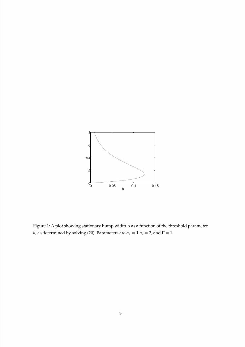
In Fig. 1 we show a typical plot of bump width ∆ as a function of the threshold parameter

h, for particular values of the other parameters. We note that the differences in timings for

the two populations do not affect the existence of stationary patterns, only their stability, as

seen below.

3.2 Stability via the Evans function

We can find the stability of stationary one-bump solutions by constructing the associatedEvans function. Evans functions were first developed to study the stability of travelling

waves in PDEs [12]. In essence the Evans function is an analytic tool whose zeros corre-

spond to eigenvalues of the linearised problem obtained after considering perturbations

around a travelling wave solution. Moreover, the order of the zero and the multiplicity of

the eigenvalue match. A recent review of their use in determining the stability of travelling

pulses in dissipative systems can be found in [25]. This theory has recently been extended to

cover travelling waves in systems with nonlocal interactions, such as studied here [26, 7, 34].

7



0 0.05 0.1 0.150

2

4

6

8

h

∆

Figure 1: A plot showing stationary bump width ∆ as a function of the threshold parameter

h, as determined by solving (20). Parameters are σe = 1 σi = 2, and Γ = 1.

8



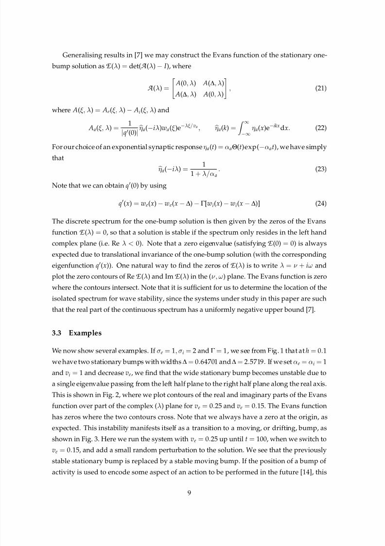
Generalising results in [7] we may construct the Evans function of the stationary one-

bump solution asE (λ) = det(A (λ) − I ), where

A (λ)= A(0, λ) A(∆, λ)

A(∆, λ) A(0, λ) , (21)

where A(ξ, λ) = Ae(ξ, λ) − Ai(ξ, λ) and

Aa(ξ, λ) =1

|q(0)| ηa(−iλ)wa(ξ)e−λξ/va , ηa(k) =

Z ∞

−∞ηa(x)e−ikx dx. (22)

For our choice of an exponential synaptic response ηa(t)= αaΘ(t)exp(−αat), we have simply

that ηa(−iλ) =1

1+ λ/αa. (23)

Note that we can obtain q(0) by using

q(x) = we(x) − we(x −∆) − Γ [wi(x) − wi(x − ∆)] (24)

The discrete spectrum for the one-bump solution is then given by the zeros of the Evans

function E (λ) = 0, so that a solution is stable if the spectrum only resides in the left hand

complex plane (i.e. Re λ < 0). Note that a zero eigenvalue (satisfying E (0) = 0) is always

expected due to translational invariance of the one-bump solution (with the corresponding

eigenfunction q(x)). One natural way to find the zeros of E (λ) is to write λ = ν + iω and

plot the zero contours of Re E (λ) and ImE (λ) in the (ν, ω) plane. The Evans function is zero

where the contours intersect. Note that it is sufficient for us to determine the location of theisolated spectrum for wave stability, since the systems under study in this paper are such

that the real part of the continuous spectrum has a uniformly negative upper bound [7].

3.3 Examples

We now show several examples. If σe = 1, σi = 2 and Γ = 1, we see from Fig. 1 that at h= 0.1

we have two stationary bumps with widths∆= 0.64701 and∆= 2.5719. If we set αe = αi = 1

and vi = 1 and decrease ve, we find that the wide stationary bump becomes unstable due to

a single eigenvalue passing from the left half plane to the right half plane along the real axis.

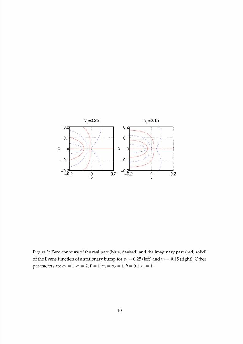
This is shown in Fig. 2, where we plot contours of the real and imaginary parts of the Evans

function over part of the complex (λ) plane for ve = 0.25 and ve = 0.15. The Evans function

has zeros where the two contours cross. Note that we always have a zero at the origin, as

expected. This instability manifests itself as a transition to a moving, or drifting, bump, as

shown in Fig. 3. Here we run the system with ve = 0.25 up until t = 100, when we switch to

ve = 0.15, and add a small random perturbation to the solution. We see that the previously

stable stationary bump is replaced by a stable moving bump. If the position of a bump of

activity is used to encode some aspect of an action to be performed in the future [14], this

9



−0.2 0 0.2−0.2

−0.1

0

0.1

0.2

ν

ω

ve=0.25

−0.2 0 0.2−0.2

−0.1

0

0.1

0.2

ν

ω

ve=0.15

Figure 2: Zero contours of the real part (blue, dashed) and the imaginary part (red, solid)

of the Evans function of a stationary bump for ve = 0.25 (left) and ve = 0.15 (right). Other

parameters are σe = 1, σi = 2,Γ = 1, αi = αe = 1, h = 0.1, vi = 1.

10



t

x

0 100 200 300 400 500 600

0

5

10

15

20

Figure 3: Instability of a stationary bump due to an eigenvalue passing through zero. At

t = 100, ve was changed from 0.25 to 0.15 (and a small random perturbation was added).

ue is plotted, red is high, blue is low. Other parameters are σe = 1, σi = 2,Γ = 1, αi = αe =

1, h= 0.1, vi = 1. The domain was discretised with 200 spatial points and periodic boundary

conditions were used.

11



instability is undesirable. For simulations of the full system we use (15) as the firing rate

function with β = 150. This moving bump will be discussed later in Sec. 4.2.

Conversely, by holding ve constant and decreasing vi we can make the wide stationary

bump in Fig. 1 go unstable through a Hopf bifurcation, in which a pair of complex eigen-

values pass through the imaginary axis. This is shown in Fig. 4, where the Evans function is

represented for vi = 0.4 (left) and vi = 0.2 (right). We see that between these values, a com-

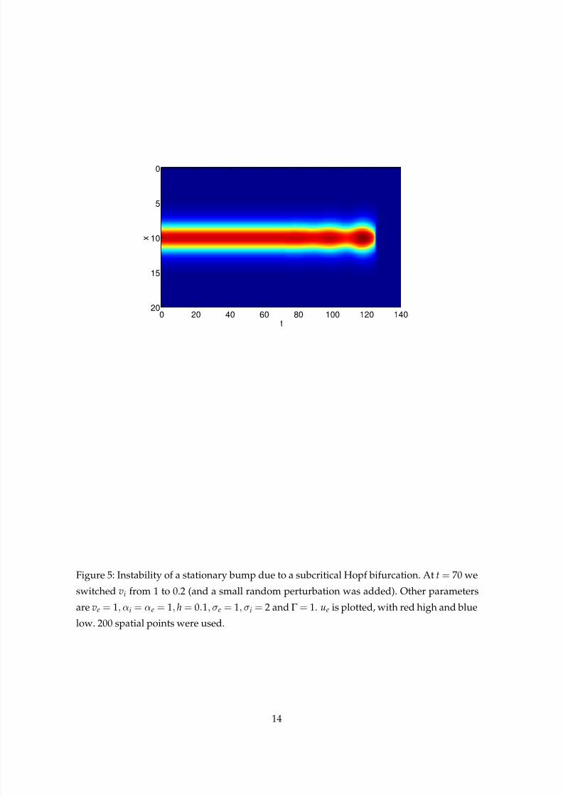
plex pair of eigenvalues moves into the right half plane. The instability is shown in Fig. 5,

where we switch vi from 1 to 0.2 halfway through the simulation. We see an oscillatory in-

stability develop, but it appears to be subcritical, and the system moves to the all-off state.

Clearly this is also undesirable in the context of working memory.

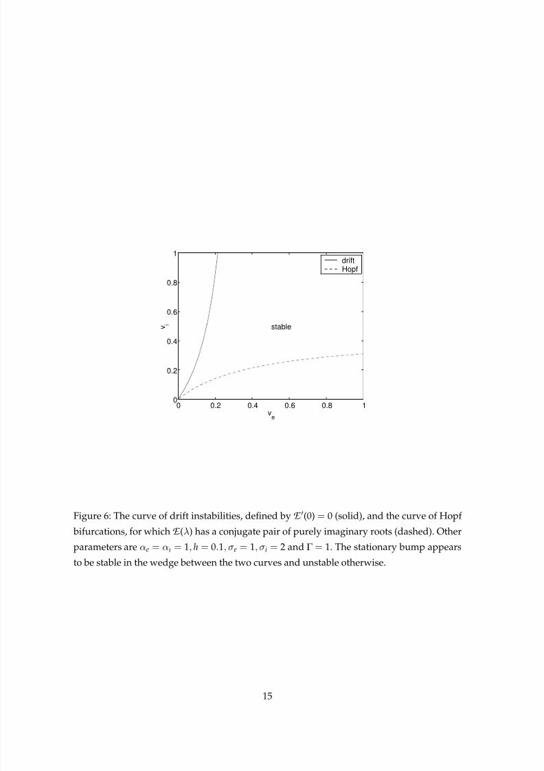
These instabilities are summarised in Fig. 6, where we plot the curves of drift instabilities

and Hopf bifurcations in the ve − vi plane. Note that we have followed only the curve

of Hopf bifurcations corresponding to the imaginary roots with smallest imaginary part.Although we have not proven it, numerical computation of the Evans function at various

points in the ve − vi plane suggests that the stationary bump is always stable in the wedge

between the two curves.

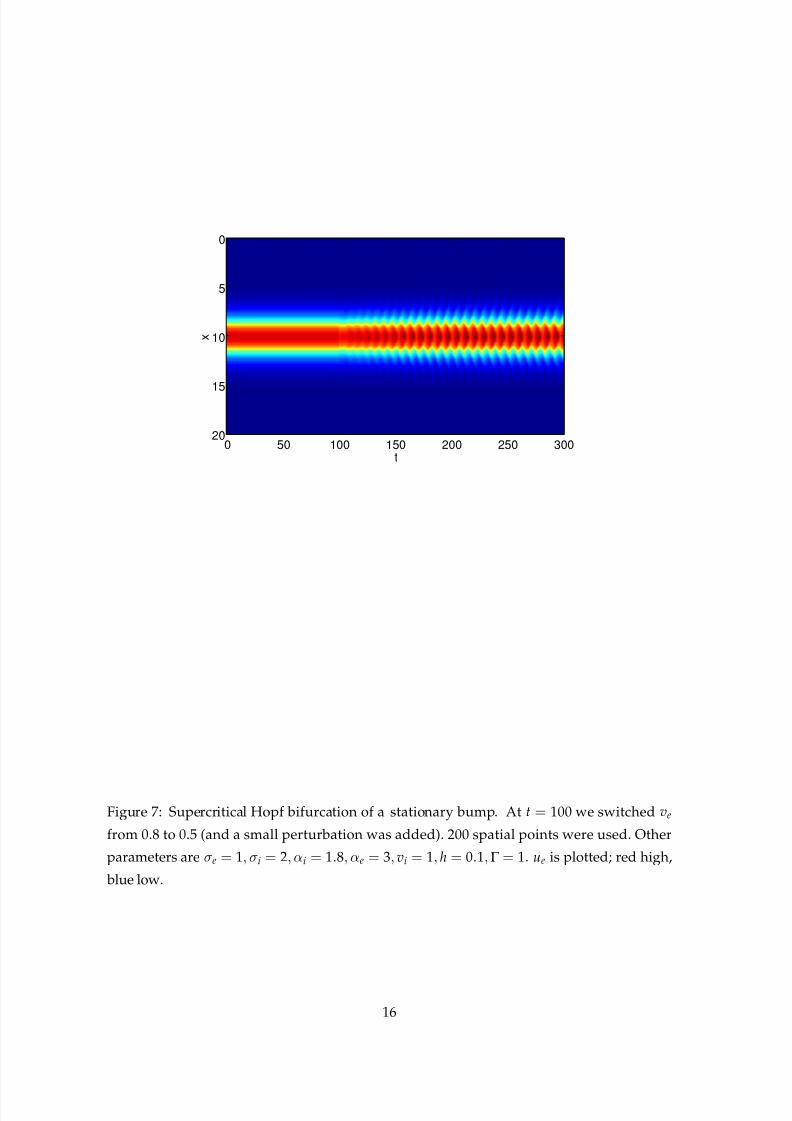
We can also find supercritical Hopf bifurcations if we relax the restriction that αi = αe =

1, i.e. if we allow different time-courses for the synaptic processing in the two populations.

In Fig. 7 we show the effect of decreasing ve from 0.8 to 0.5, where αi = 1.8 and αe = 3.

Oscillations appear, and their amplitude rapidly saturates. Presumably, by changing other

parameters it would be possible to observe higher codimension bifurcations, such as the

Takens-Bogdanov (double zero eigenvalue) [9].

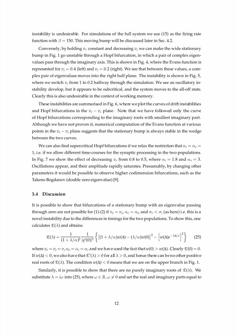
3.4 Discussion

It is possible to show that bifurcations of a stationary bump with an eigenvalue passing

through zero are not possible for (1)-(2) if ve = vi, αe = αi, and σe < σi (as here) i.e. this is a

novel instability due to the differences in timings for the two populations. To show this, one

calculatesE (λ) and obtains

E (λ) = 1(1+ λ/α)2 1

|q(0)|2 (1+ λ/α)w(∆) − (λ/α)w(0)2 − w(∆)e−λ∆/v2 (25)

where ve = vi = v, αe = αi = α, and we have used the fact that w(0) > w(∆). ClearlyE (0)= 0.

If w(∆) < 0, we also have thatE (λ) > 0 for all λ > 0, and hence there can be no other positive

real roots of E (λ). The condition w(∆) < 0 means that we are on the upper branch in Fig. 1.

Similarly, it is possible to show that there are no purely imaginary roots of E (λ). We

substitute λ= iω into (25), where ω ∈ R, ω = 0 and set the real and imaginary parts equal to

12



−0.4 −0.2 0 0.2−0.4

−0.2

0

0.2

0.4

ν

ω

vi=0.4

−0.4 −0.2 0 0.2−0.4

−0.2

0

0.2

0.4

ν

ω

vi=0.2

Figure 4: Zero contours of the real part (blue, dashed) and the imaginary part (red, solid)

of the Evans function for a stationary bump for vi = 0.4 (left) and vi = 0.2 (right). Other

parameters are ve = 1, αi = αe = 1, h = 0.1, σe = 1, σi = 2 and Γ = 1.

13



t

x

0 20 40 60 80 100 120 140

0

5

10

15

20

Figure 5: Instability of a stationary bump due to a subcritical Hopf bifurcation. At t= 70 we

switched vi from 1 to 0.2 (and a small random perturbation was added). Other parameters

are ve = 1, αi = αe = 1, h= 0.1, σe = 1, σi = 2 and Γ = 1. ue is plotted, with red high and blue

low. 200 spatial points were used.

14



0 0.2 0.4 0.6 0.8 1

0

0.2

0.4

0.6

0.8

1

ve

v i

stable

drift

Hopf

Figure 6: The curve of drift instabilities, defined by E (0) = 0 (solid), and the curve of Hopf

bifurcations, for which E (λ) has a conjugate pair of purely imaginary roots (dashed). Other

parameters are αe = αi = 1, h = 0.1, σe = 1, σi = 2 and Γ = 1. The stationary bump appears

to be stable in the wedge between the two curves and unstable otherwise.

15



t

x

0 50 100 150 200 250 300

0

5

10

15

20

Figure 7: Supercritical Hopf bifurcation of a stationary bump. At t = 100 we switched ve

from 0.8 to 0.5 (and a small perturbation was added). 200 spatial points were used. Other

parameters are σe = 1, σi = 2, αi = 1.8, αe = 3, vi = 1, h = 0.1,Γ = 1. ue is plotted; red high,

blue low.

16



zero, obtaining

[w(∆)]2(1 − cos θ) − (ω/α)2[w(∆) − w(0)]2= 0 (26)

w(∆){w(∆)sin θ − 2(ω/α)[w(∆) − w(0)]} = 0 (27)

where θ = 2ω∆/v. Assuming that w(∆) = 0, solving (27) for w(∆) − w(0) and substituting

into (26) we obtain

[w(∆)]2

1 − cos θ − (1/4)sin2 θ= 0 (28)

which is only true if θ = 0, 2π, 4π . . . Substituting these values of θ back into (27) we see that

it cannot simultaneously be satisfied, i.e.E (λ) has no purely imaginary roots. If w(∆)= 0 the

only root of E (λ) is λ = 0, which corresponds to the saddle-node bifurcation in Fig. 1. Thus

both types of instabilities are a result of the differences in timings for the two populations.

Bifurcations of the types discussed in this section have recently been observed in a sys-

tem with one neural population but in which the threshold is a dynamic variable [8]. There,

the authors also saw a stationary bump start to move as an eigenvalue moved through zero,

and stationary breathers caused by a supercritical Hopf bifurcation. Breathers have also

been observed in neural field equations by Bressloff et al. [4, 13], but in those papers the au-

thors made the domain inhomogeneous, inducing a bump to occur over a spatially-localised

input. During normal awake operation the cortex continuously receives inhomogeneous in-

puts, so the response of a neural model with such inputs is of interest. However, under

general anaesthesia the cortex will receive less input (and conduction velocities may be in-

creased [40]) so it is also of interest to study the existence and stability of patterns in thissituation.

Blomquist et al. [1] recently studied a two-layer neural field model that can be best

thought of as a generalisation of that studied by Pinto and Ermentrout [33]. In contrast

with Pinto and Ermentrout, Blomquist et al. included inhibitory-to-inhibitory connections

and did not assume that the firing rate function for the inhibitory population was linear.

They did not include conduction delays, but obtained both stable and unstable breathers

that were created in Hopf bifurcations, as seen here.

The common theme between our results and those of Coombes and Owen [8], Bress-

loff et al. [4, 13] and Blomquist et al. [1] is the presence of a second variable describing either

another population of neurons or a local field such as an adaptation current.

4 Travelling wave solutions

We now discuss travelling wave solutions, both fronts (which connect a region of high activ-

ity to one of low activity) and pulses (travelling bumps, before and after which the medium

is quiescent). We introduce the coordinate ξ = x − ct and seek functions U(ξ, t)= u(x − ct, t)

17



that satisfy the full integral model equations. In the (ξ, t) coordinates, these integral equa-

tions can be expressed as U(ξ, t) =Ue(ξ, t) − Ui(ξ, t), with

Ua(ξ, t) =Z ∞

−∞d ywa( y)

Z ∞

0dsηa(s) f ◦ U(ξ − y+ cs+ c| y|/va, t − s − | y|/va). (29)

The travelling wave is a stationary solution U(ξ, t) = q(ξ) (independent of t), that satisfies

q(ξ) = qe(ξ) − qi(ξ), with

qa(ξ) =Z ∞

0dsηa(s)ψa(ξ + cs), (30)

where

ψa(ξ) =Z ∞

−∞d ywa( y) f ◦ q(ξ − y+ c| y|/va). (31)

4.1 Fronts

We look for travelling front solutions such that q(ξ) > h for ξ < 0 and q(ξ) < h for ξ > 0. It isthen a simple matter to show that (for the special case of the Heaviside firing rate function

chosen earlier)

ψa(ξ) =

R ∞

ξ/(1−c/va) d ywa( y) = Γ a exp(m−a ξ)/2 ξ ≥ 0

R ∞ξ/(1+c/va) d ywa( y) = Γ a

1 − exp(m+

a ξ)/2

ξ < 0, m±

a =ωa

c ± va(32)

The choice of origin, q(0) = h, gives an implicit equation for the speed of the wave as a

function of system parameters:

2h=

1

1 − cm−e /αe −

Γ

1 − cm−i /αi c ≥ 0 (33)

2h = 2(1 − Γ )+Γ

1 − cm+

i /αi−

1

1 − cm+e /αe

c < 0 (34)

Both equations may be written as quadratic equations in c. To ensure that limξ→−∞ q(ξ) > h,

we must haveR R

w( y)d y = 1 − Γ > h. We note that a standing front (c = 0) occurs when

2h = 1 − Γ . Also, it is not necessary to have different propagation velocities and synaptic

processing time-constants for such fronts to exist; they are seen robustly in simpler systems

where these parameters are equal [32].

Once again the Evans function is easily obtained using the techniques described in [7]and may be written in the form

E (λ) = 1 −H (λ)

H (0), (35)

where H (λ) = H e(λ) −H i(λ) and

H a(λ) =Z ∞

0d ywa( y)ηa( y/c − y/va)e−λ y/c. (36)

For the exponential synaptic response we have simply that

H a(λ) =αaΓ a

2σa 1

σa

+αa1

c

−1

va+λ

c −1

. (37)

18



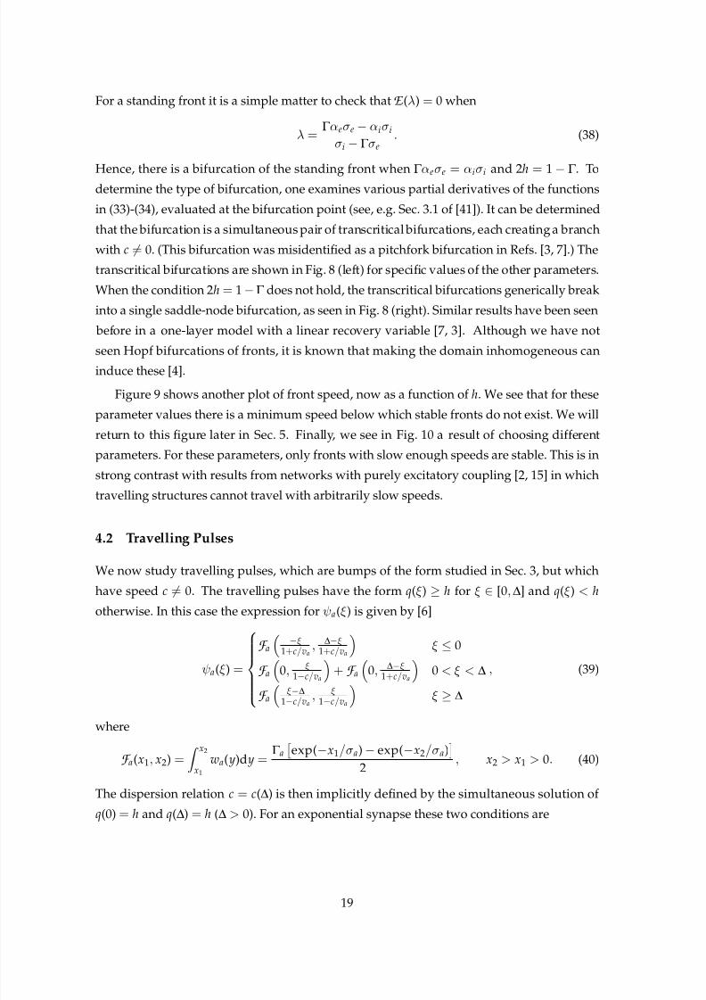
For a standing front it is a simple matter to check that E (λ) = 0 when

λ =Γ αeσe − αiσi

σi − Γ σe. (38)

Hence, there is a bifurcation of the standing front whenΓ

αeσe=

αiσi and 2h=

1 −Γ

. Todetermine the type of bifurcation, one examines various partial derivatives of the functions

in (33)-(34), evaluated at the bifurcation point (see, e.g. Sec. 3.1 of [41]). It can be determined

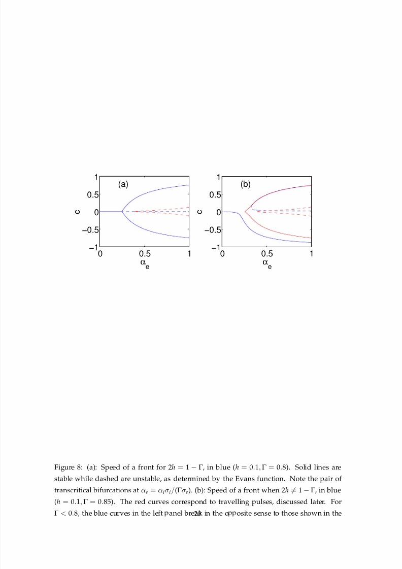
that the bifurcation is a simultaneous pair of transcritical bifurcations, each creating a branch

with c = 0. (This bifurcation was misidentified as a pitchfork bifurcation in Refs. [3, 7].) The

transcritical bifurcations are shown in Fig. 8 (left) for specific values of the other parameters.

When the condition 2h= 1 −Γ does not hold, the transcritical bifurcations generically break

into a single saddle-node bifurcation, as seen in Fig. 8 (right). Similar results have been seen

before in a one-layer model with a linear recovery variable [7, 3]. Although we have not

seen Hopf bifurcations of fronts, it is known that making the domain inhomogeneous caninduce these [4].

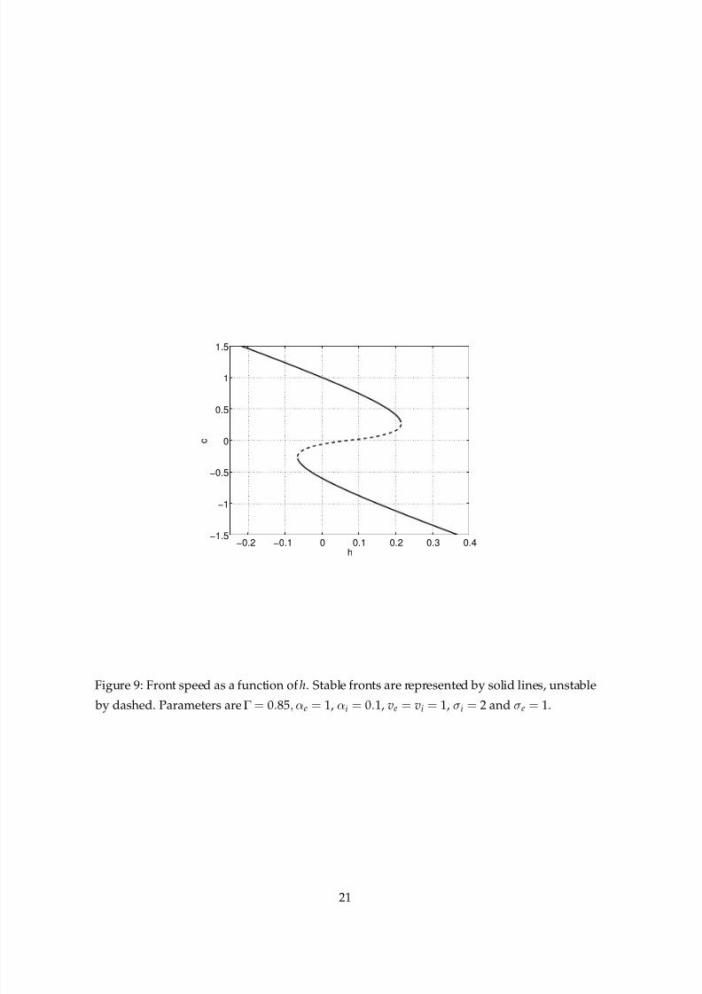
Figure 9 shows another plot of front speed, now as a function of h. We see that for these

parameter values there is a minimum speed below which stable fronts do not exist. We will

return to this figure later in Sec. 5. Finally, we see in Fig. 10 a result of choosing different

parameters. For these parameters, only fronts with slow enough speeds are stable. This is in

strong contrast with results from networks with purely excitatory coupling [2, 15] in which

travelling structures cannot travel with arbitrarily slow speeds.

4.2 Travelling Pulses

We now study travelling pulses, which are bumps of the form studied in Sec. 3, but which

have speed c = 0. The travelling pulses have the form q(ξ) ≥ h for ξ ∈ [0,∆] and q(ξ) < h

otherwise. In this case the expression for ψa(ξ) is given by [6]

ψa(ξ) =

F a

−ξ

1+c/va, ∆−ξ

1+c/va

ξ ≤ 0

F a

0, ξ

1−c/va

+F a

0, ∆−ξ

1+c/va

0 < ξ < ∆

F a ξ−∆

1−c/va ,

ξ

1−c/va ξ ≥∆

, (39)

where

F a(x1, x2) =Z x2

x1

wa( y)d y =Γ a

exp(−x1/σa) − exp(−x2/σa)

2

, x2 > x1 > 0. (40)

The dispersion relation c = c(∆) is then implicitly defined by the simultaneous solution of

q(0)= h and q(∆) = h (∆ > 0). For an exponential synapse these two conditions are

19





−0.2 −0.1 0 0.1 0.2 0.3 0.4−1.5

−1

−0.5

0

0.5

1

1.5

h

c

Figure 9: Front speed as a function of h. Stable fronts are represented by solid lines, unstable

by dashed. Parameters are Γ = 0.85, αe = 1, αi = 0.1, ve = vi = 1, σi = 2 and σe = 1.

21



−0.2 −0.1 0 0.1 0.2 0.3 0.4 0.5

−1.5

−1

−0.5

0

0.5

1

1.5

h

c

Figure 10: Front speed as a function of h. Parameters are αi = αe = 1, ve = vi = 1, σe = 1, σi =

2,Γ = 0.8. The solid branch is stable, while the dashed ones are unstable.

22



2h = 2(1 − Γ )+ 2Γ exp(−αi∆/c) − exp(−αe∆/c)

+

exp(−αe∆/c) − 1

1 − cm−e /αe +

exp(−αe∆/c) − exp(−m+e ∆)

1 − cm+

e /αe −Γ

exp(−αi∆/c) − 1

1 − cm−i /αi

−Γ

exp(−αi∆/c) − exp(−m+

i ∆)

1 − cm+

i /αi

(41)

2h =

1 − exp(m−

e ∆)

1 − cm−e /αe

− Γ

1 − exp(m−

i ∆)

1 − cm−i /αi

(42)

Note that as c → 0, both (41) and (42) reduce to the equation governing the width of a

stationary bump, (20), as expected.

The Evans function takes the same form as in Sec. 3.2, with (21) replaced by

A (λ) = A(0, λ) B(0, λ)

A(∆, λ) B(∆, λ)

. (43)

where A(ξ, λ) = Ae(ξ, λ) − Ai(ξ, λ), B(ξ, λ) = Be(ξ, λ) − Bi(ξ, λ), and

Aa(ξ, λ) =1

c|q(0)|

Z ∞

ξ/(1−c/va)d ywa( y)ηa(−ξ/c+ y/c − y/va)e−λ( y−ξ)/c (44)

Ba(ξ, λ) =1

c|q(∆)|

Z ∞

(ξ−∆)/(1+c/va)d ywa( y)ηa((∆ − ξ)/c+ y/c − | y|/va)e−λ( y−(ξ−∆))/c. (45)

Explicitly, we have

Aa(0, λ) = αaΓ a

2|q(0)|(c − αa/m−a + λσa)

(46)

Aa(∆, λ) = exp[−∆(va + σaλ)/(σa(va − c))] Aa(0, λ), (47)

Ba(0, λ) =αaΓ a

2|q(∆)|

exp[−∆(αa + λ)/c] − exp[−∆(va + λσa)/(σa(va + c))]

c − αa/m+a − λσa

+exp[−∆(αa + λ)/c]

c − αa/m−a + λσa

(48)

B(∆, λ) =

q(0)

q(∆)

A(0, λ), (49)

Note that as c → 0, the matrix (43) reduces to the matrix associated with the stability of

a stationary bump, (21), as expected. To evaluate the derivatives of q in (46)-(49) we use

q= q

e − qi, where q

a = αa(qa − ψa)/c. Specifically, we have

ψa(0) = Γ a[1 − exp(−m+a ∆)]/2, ψa(∆) = Γ a[1 − exp(m−a ∆)]/2, (50)

qa(0) = Γ a

1 − exp(−αa∆/c)+

1 − exp(−αa∆/c)

2(cm−a /αa − 1)

+exp(−m+a ∆) − exp(−αa∆/c)

2(cm+a /αa − 1)

(51)

and

qa(∆) =Γ a[1 − exp(m−

a ∆)]

2(1 − cm−

a /αa)

(52)

23



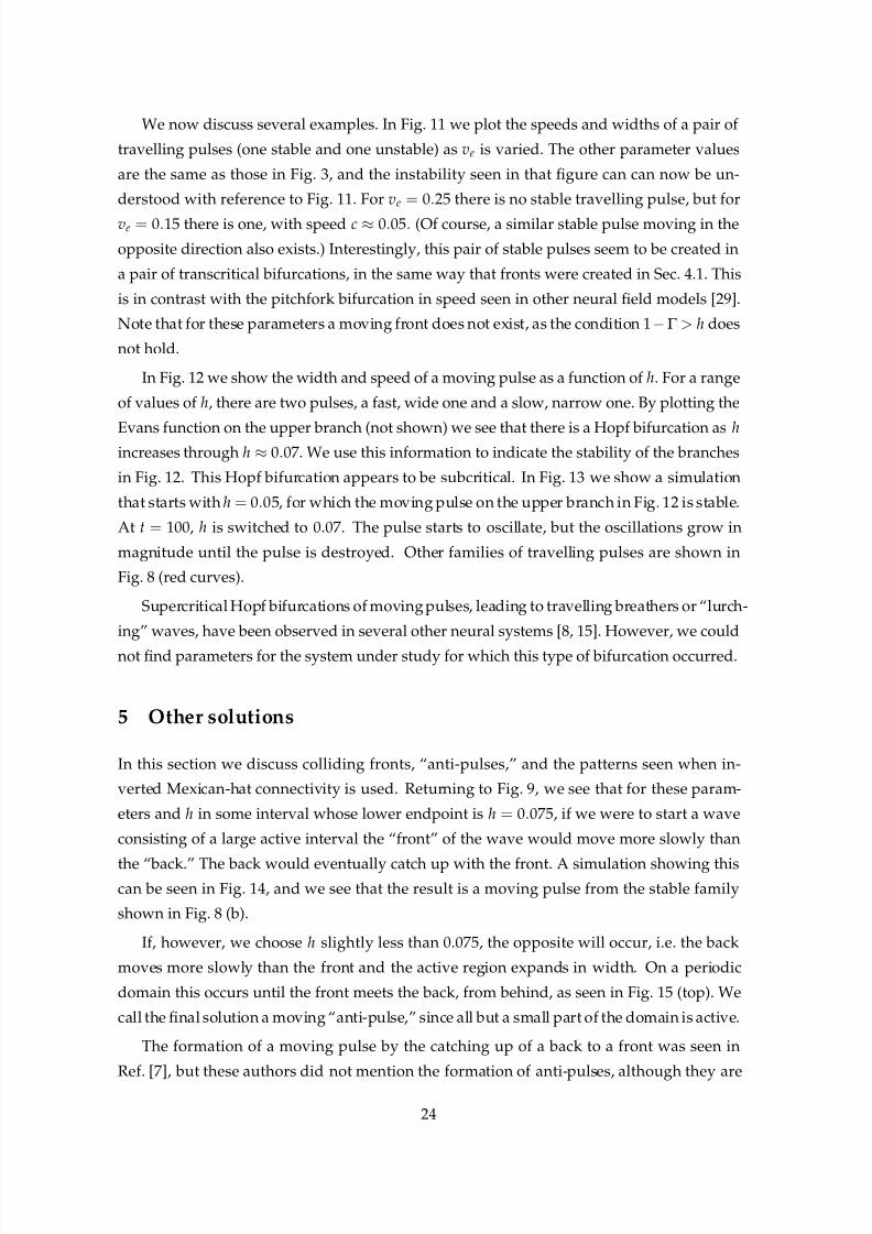
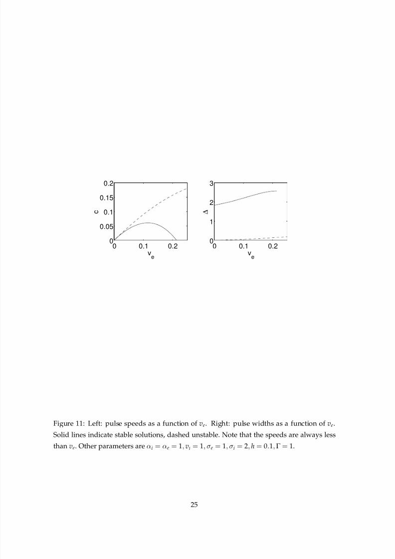
We now discuss several examples. In Fig. 11 we plot the speeds and widths of a pair of

travelling pulses (one stable and one unstable) as ve is varied. The other parameter values

are the same as those in Fig. 3, and the instability seen in that figure can can now be un-

derstood with reference to Fig. 11. For ve = 0.25 there is no stable travelling pulse, but for

ve = 0.15 there is one, with speed c ≈ 0.05. (Of course, a similar stable pulse moving in the

opposite direction also exists.) Interestingly, this pair of stable pulses seem to be created in

a pair of transcritical bifurcations, in the same way that fronts were created in Sec. 4.1. This

is in contrast with the pitchfork bifurcation in speed seen in other neural field models [29].

Note that for these parameters a moving front does not exist, as the condition 1 −Γ > h does

not hold.

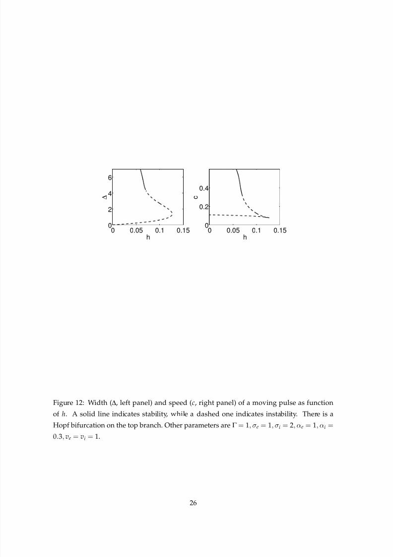
In Fig. 12 we show the width and speed of a moving pulse as a function of h. For a range

of values of h, there are two pulses, a fast, wide one and a slow, narrow one. By plotting the

Evans function on the upper branch (not shown) we see that there is a Hopf bifurcation as hincreases through h ≈ 0.07. We use this information to indicate the stability of the branches

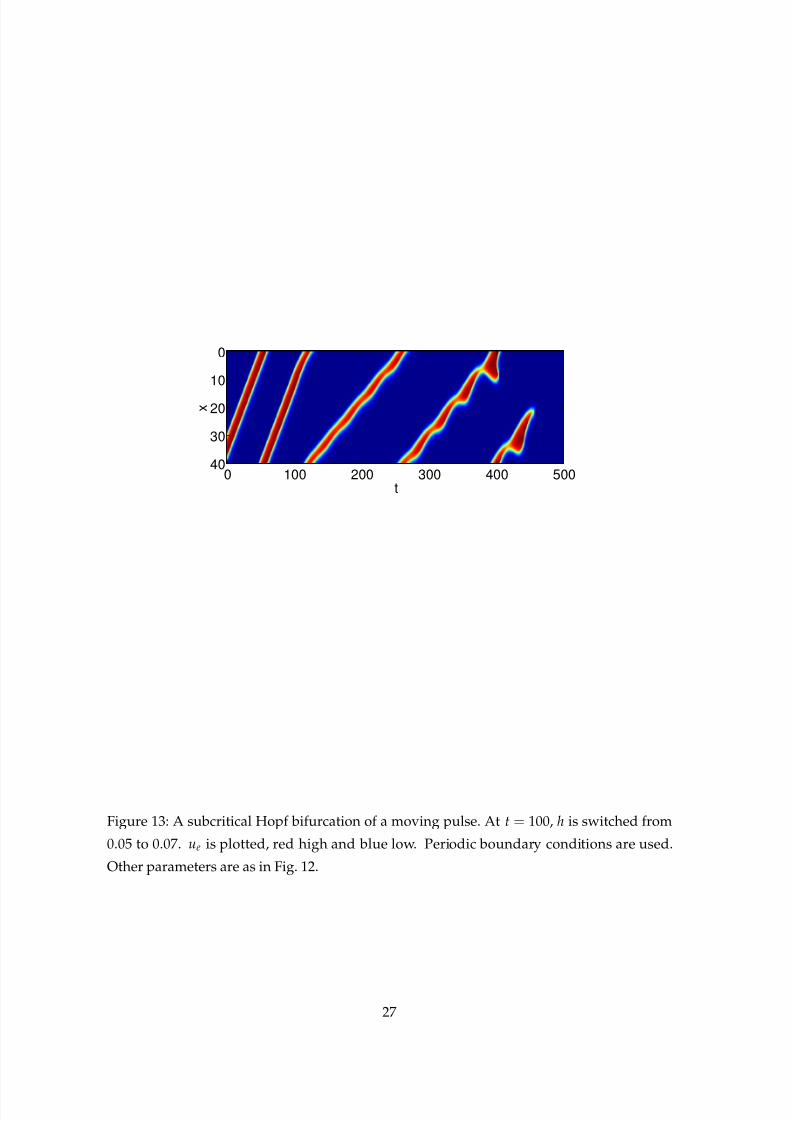
in Fig. 12. This Hopf bifurcation appears to be subcritical. In Fig. 13 we show a simulation

that starts with h= 0.05, for which the moving pulse on the upper branch in Fig. 12 is stable.

At t = 100, h is switched to 0.07. The pulse starts to oscillate, but the oscillations grow in

magnitude until the pulse is destroyed. Other families of travelling pulses are shown in

Fig. 8 (red curves).

Supercritical Hopf bifurcations of moving pulses, leading to travelling breathers or “lurch-

ing” waves, have been observed in several other neural systems [8, 15]. However, we could

not find parameters for the system under study for which this type of bifurcation occurred.

5 Other solutions

In this section we discuss colliding fronts, “anti-pulses,” and the patterns seen when in-

verted Mexican-hat connectivity is used. Returning to Fig. 9, we see that for these param-

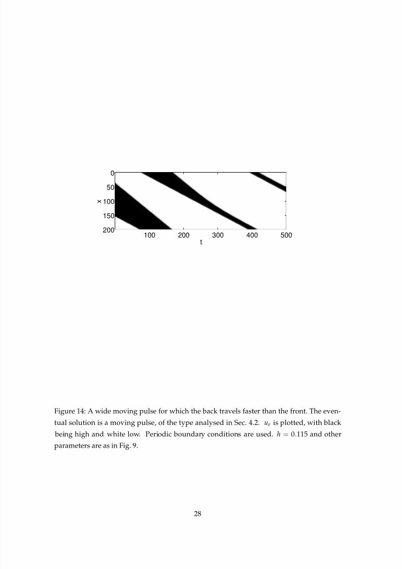
eters and h in some interval whose lower endpoint is h = 0.075, if we were to start a wave

consisting of a large active interval the “front” of the wave would move more slowly than

the “back.” The back would eventually catch up with the front. A simulation showing thiscan be seen in Fig. 14, and we see that the result is a moving pulse from the stable family

shown in Fig. 8 (b).

If, however, we choose h slightly less than 0.075, the opposite will occur, i.e. the back

moves more slowly than the front and the active region expands in width. On a periodic

domain this occurs until the front meets the back, from behind, as seen in Fig. 15 (top). We

call the final solution a moving “anti-pulse,” since all but a small part of the domain is active.

The formation of a moving pulse by the catching up of a back to a front was seen in

Ref. [7], but these authors did not mention the formation of anti-pulses, although they are

24



0 0.1 0.20

0.05

0.1

0.15

0.2

ve

c

0 0.1 0.20

1

2

3

ve

∆

Figure 11: Left: pulse speeds as a function of ve. Right: pulse widths as a function of ve.

Solid lines indicate stable solutions, dashed unstable. Note that the speeds are always less

than ve. Other parameters are αi = αe = 1, vi = 1, σe = 1, σi = 2, h = 0.1,Γ = 1.

25



0 0.05 0.1 0.150

0.2

0.4

h

c

0 0.05 0.1 0.150

2

4

6

h

∆

Figure 12: Width (∆, left panel) and speed (c, right panel) of a moving pulse as function

of h. A solid line indicates stability, while a dashed one indicates instability. There is a

Hopf bifurcation on the top branch. Other parameters are Γ = 1, σe = 1, σi = 2, αe = 1, αi =

0.3, ve = vi = 1.

26



t

x

0 100 200 300 400 500

0

10

20

30

40

Figure 13: A subcritical Hopf bifurcation of a moving pulse. At t = 100, h is switched from

0.05 to 0.07. ue is plotted, red high and blue low. Periodic boundary conditions are used.

Other parameters are as in Fig. 12.

27



t

x

100 200 300 400 500

0

50

100

150

200

Figure 14: A wide moving pulse for which the back travels faster than the front. The even-

tual solution is a moving pulse, of the type analysed in Sec. 4.2. ue is plotted, with black

being high and white low. Periodic boundary conditions are used. h = 0.115 and other

parameters are as in Fig. 9.

28



most certainly expected even when ve = vi and αe = αi. We now analyse anti-pulses.

5.1 Anti-pulses

For anti-pulses, q(ξ) < h for 0 < ξ < ∆ and q(ξ) > h otherwise. UsingR

∞−∞ wa(x)dx = Γ a, wehave

ψa(ξ) =

Γ a −F a

−ξ

1+c/va, ∆−ξ

1+c/va

ξ ≤ 0

Γ a −F a

0, ξ

1−c/va

−F a

0, ∆−ξ

1+c/va

0 < ξ < ∆

Γ a −F a

ξ−∆

1−c/va, ξ

1−c/va

ξ ≥ ∆

, (53)

where F a is given by (40). The conditions q(0) = h = q(∆) are then easily determined using

q(ξ) = qe(ξ) − qi(ξ) and

qa(ξ) =Z ∞

0ηa(s)ψa(ξ + cs)ds (54)

and the fact that these integrals have essentially been done in the determination of (41)-(42).

They are

2h = −2Γ exp(−αi∆/c) − exp(−αe∆/c)

−

exp(−αe∆/c) − 1

1 − cm−e /αe

−

exp(−αe∆/c) − exp(−m+

e ∆)

1 − cm+e /αe

+Γ

exp(−αi∆/c) − 1

1 − cm−i /αi

+ Γ

exp(−αi∆/c) − exp(−m+i ∆)

1 − cm+

i/αi

(55)

and

2h=

2(1 −Γ

) − 1 − exp(m−e ∆)

1 − cm−e /αe +Γ 1 − exp(m−i ∆)

1 − cm−i /αi (56)

The width and speed of anti-pulses is determined by the simultaneous solution of (55)-(56).

The Evans function for antipulses has the same form as that for pulses, since only the fact

that q(0) = q(∆) = h is used, the sign of q(ξ) − h for ξ ∈ (0,∆) being irrelevant.

In fact, the analysis of anti-pulses does not bring any new results, as the system under

study is symmetric about the “balanced” parameter point 2h = 1 − Γ , at which there are

stationary fronts (see Sec. 4.1). If we make the replacement h → 1 − Γ − h in (55)-(56), we

obtain (41)-(42), and vice versa. Thus, for a given value of h, say h∗, at which there exists

a pulse, there exists a corresponding antipulse when h = 1 − Γ − h∗ (all other parameters

being the same). It will have the same width (as determined by the zeros of q(ξ) − h), speed

and stability as the pulse.

5.2 Inverted Mexican hat connectivity

Although much work on pattern formation in neural field models has used one layer of

neurons with Mexican-hat connectivity, for which inhibitory connections have a wider spa-

tial extent than excitatory, there is evidence that the opposite is true, at least in some con-

texts [39]. We now briefly analyse (1)-(2) with coupling function (4), but with σe

> σi,

29



t

x

100 200 300 400 500 600

0

50

100

150

200

0 50 100 150 200

−0.5

0

0.5

x

u

Figure 15: A wide moving pulse for which the back travels slower than the front, leading

to the formation of an “anti-pulse”. Top: ue is plotted, with black being high and white

low. Bottom: u = ue − ui once the anti-pulse has formed. h = 0.05, so most of the domain is

active. Other parameters are as in Fig. 9.

30



i.e. with the excitatory connections having a greater spatial extent than the inhibitory, which

we refer to as inverted Mexican-hat connectivity.

As before, we can find families of moving pulses. In Fig. 16 we show solutions of (41)-

(42) as h is varied for inverted Mexican-hat connectivity. Note that not every point on the

curves in Fig. 16 corresponds to a one-pulse solution, as some of the solutions may have

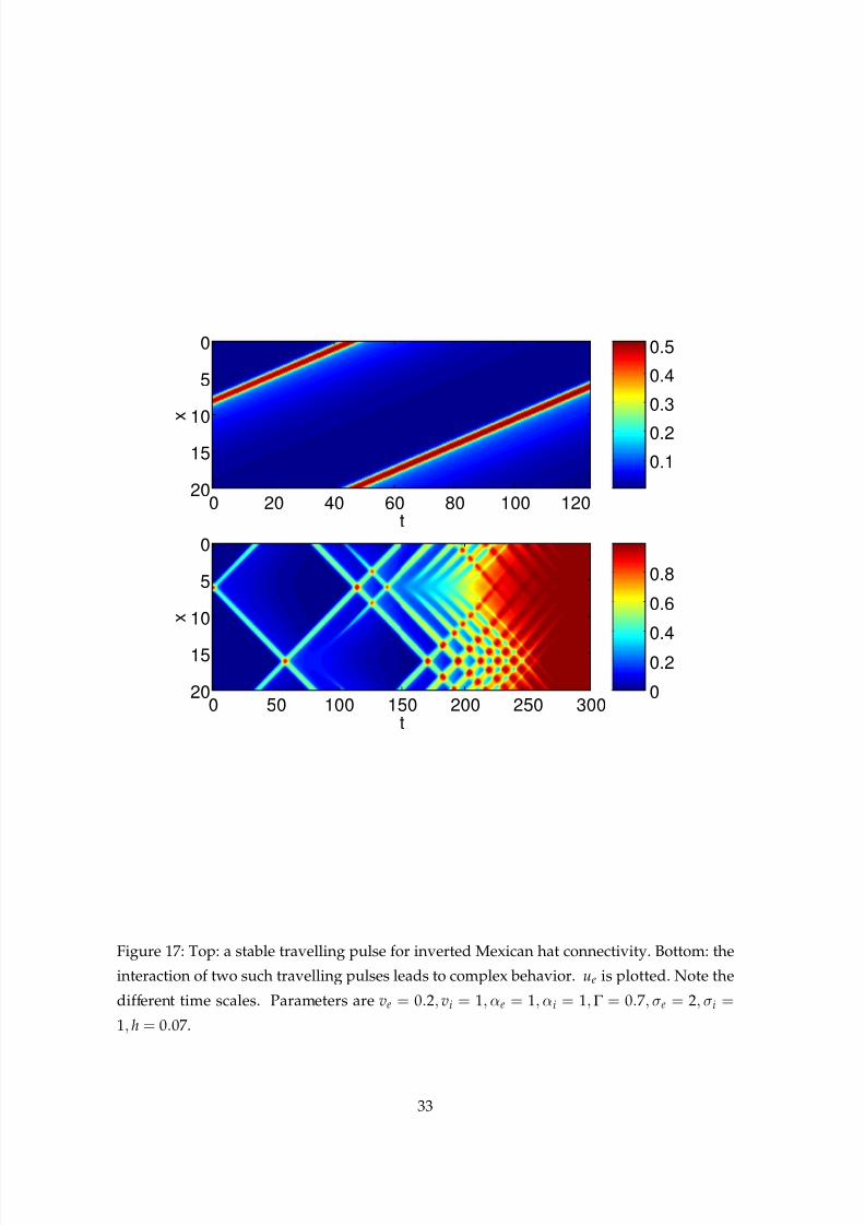
q(ξ) > h for more than one interval. In Fig. 17 we show a stable travelling one-pulse solution

from the curve in Fig. 16 (top panel), and the complex transients that can occur when two

such pulses interact (bottom panel, same parameters). For this connectivity, we can also

obtain families of travelling fronts (not shown).

6 Discussion

We have studied stationary and travelling bump and front solutions of a two-layer neural

field model with different conduction velocities and synaptic processing time-constants for

the two populations. By varying these parameters we have found bifurcations of stationary

bumps to both travelling and breathing bumps. These bifurcations can be found by explic-

itly constructing an Evans function for these solutions and, as shown in Sec. 3.4, they cannot

occur if the synaptic time-constants and conduction velocities are the same for both layers.

Our work has produced results similar to those of several other groups. For example,

Curtu and Ermentrout [9] recently studied an extension of the system first discussed by

Hansel and Sompolinsky [19]. This model had one neural population, Mexican-hat type

connectivity, an adaptation variable and no delays. The authors found travelling and stand-

ing waves, and stationary, spatially-periodic patterns. However, their results were derived

by linearising about the spatially-uniform state, and are thus unable to say anything regard-

ing spatially-localised patterns of the type studied here.

Golomb and Ermentrout [15] studied the effects of delays on propagating activity. They

included a fixed delay and found that increasing this led to lurching waves. (We did not

include a fixed delay, but see below.) However, they used a spiking neural network in which

each neuron could only fire once, and only excitatory coupling. Because of this, they could

not find stationary or arbitrarily slowly moving patterns, as we have. In later work [16, 17]

these authors studied a network with both excitatory and inhibitory populations but did

not include conduction delays for most of their analysis, and still allowed neurons to fire at

most once, thus precluding the existence of stationary patterns. One interesting result that

they found was the coexistence of both fast and slow propagating pulses, which we have

not found. However, these authors found that once neurons were allowed to fire multiple

times this bistability disappeared, with only the slow pulses persisting.

Blomquist et al. [1] studied a two-layer neuronal network without delays (an extension

of that studied by Pinto and Ermentrout [33]), and found both subcritical and supercritical

31



0 0.05 0.10.12

0.14

0.16

0.18

h

c

0 0.05 0.10

2

4

6

h

∆

Figure 16: Width (left panel) and speed (right panel) of a travelling pulse as a function of

h, with inverted Mexican hat connectivity. Solid lines represent stable one-bump solutions

and dashed unstable, while the dotted lines indicate a solution of (41)-(42) which is not a

one-bump solution. Parameters are ve = 0.2, vi = 1, αe = 1, αi = 1,Γ = 0.7, σe = 2, σi = 1.

32



0.1

0.2

0.3

0.4

0.5

t

x

0 50 100 150 200 250 300

0

5

10

15

20

t

x

0 20 40 60 80 100 120

0

5

10

15

20

0

0.2

0.4

0.6

0.8

Figure 17: Top: a stable travelling pulse for inverted Mexican hat connectivity. Bottom: the

interaction of two such travelling pulses leads to complex behavior. ue is plotted. Note the

different time scales. Parameters are ve = 0.2, vi = 1, αe = 1, αi = 1,Γ = 0.7, σe = 2, σi =

1, h = 0.07.

33



Hopf bifurcations of stationary bumps. Coombes and Owen [8] studied a single neural

layer with Mexican-hat connectivity and a variable representing spike frequency adaptation.

They found both drifting and breathing bifurcations of stationary bumps, as we have, and

also supercritical Hopf bifurcations of travelling bumps, which we have not found. We now

discuss possible extensions of the work presented here.

One extension would be to break the homogeneity of the domain (reflected by the ap-

pearance of x and y in (2) in only the combination x − y) as Jirsa and Kelso have done [24],

but for the system studied here. These authors modelled heterogeneity by putting a direct

connection from one part of the domain to another and studied the effect of varying the

length of this connection.

Roxin et al. [35] recently studied a generalisation of a neural field model first presented

by Hansel and Sompolinsky [19] in which there is a fixed delay in the nonlinear term, as op-

posed to the space-dependent delays that we have. This delay is meant to mimic those dueto synaptic and dendritic processing. These authors found a wide variety of spatiotemporal

patterns. Including such a term in our equations would involve replacing u(x − y, t − | y|/va)

in (2) by u(x − y, t − | y|/va − D), where D is a fixed positive delay. As mentioned above, this

type of delay was studied by Golomb and Ermentrout [15]. As an example of the effect of

including such a term, it is straightforward to show that the equations governing the speed

of a front (33)-(34) would be modified to

2h =exp(Dcm−

e )

1 − cm−e /αe

−Γ exp(Dcm−

i )

1 − cm−

i

/αic ≥ 0 (57)

2h = 2(1 −Γ )+Γ exp(Dcm+

i )

1 − cm+

i /αi−

exp(Dcm+e )

1 − cm+e /αe

c < 0 (58)

and it seems likely that all of the calculations performed here could also be done with such

a term included. Hutt [21] discussed a similar idea, but wrote the nonlinear term in (2) as

a linear combination of a term whose delay depends on distance and one whose delay is

fixed.

Further extensions could include verifying some of the predictions here with a network

of spiking neurons. This would be computationally intensive due to the inclusion of de-

lays, but similar work has been performed [15]. An important extension that would make

more valid the results here and elsewhere [7, 8], would be to derive similar results for a con-

tinuous firing rate function, f [9]. Also important is the consideration of a two-dimensional

domain since the cortex is best thought of as a two-dimensional sheet of interconnected neu-

rons. There have been recent results on patterns (multi-bump solutions, breathers and spiral

waves) in two-dimensional neural fields [30, 13, 28], but none of these models have included

even one conduction velocity or delay. While it seems that including a finite conduction ve-

locity does not destabilise travelling bumps or fronts in one spatial dimension [5, 15], it is

not clear whether the same holds in two dimensions.

34



A more general model, more clearly differentiating the two neural populations, would

be

ua = ηa ∗ ψa, a ∈ {e, i} (59)

ψe(x, t) =Z ∞

−∞ d ywee( y) f e ◦ ue(x − y, t − | y|/ve)

−Z ∞

−∞d ywie( y) f i ◦ ui(x − y, t − | y|/vi) (60)

ψi(x, t) =Z ∞

−∞d ywei( y) f e ◦ ue(x − y, t − | y|/ve)

−Z ∞

−∞d ywii( y) f i ◦ ui(x − y, t − | y|/vi) (61)

Here we not only have different conduction velocities ve and vi and different synaptic filters

ηe and ηi, but different firing rate functions f e and f i and four coupling functions, wee, wei, wie

and wii instead of the two in (1)-(2). Choosing f a(u) = Θ(u − ha), i.e. using the Heaviside

function as the firing rate function, with two different thresholds, we should be able to

analyse (59)-(61) in much the same way as we have analysed (1)-(2) in this paper. Some of

the analysis in [8], in which the threshold is a dynamic variable, should be applicable to

the analysis of (59)-(61) when he = hi. The model (1)-(2) can be considered as intermediate

between (59)-(61) and previous models in which there is only one population of neurons,

one synaptic filter, and one conduction velocity [6, 7].

Guo et al. [18] have recently studied a pair of coupled delay-differential equations that

are similar in structure to (59)-(61), as have Shayer and Campbell [36], although those sys-

tems have no spatial structure. Note that after setting ve=

vi=

∞ in (60)-(61) and choosingηe(t) = Θ(t)e−t and ηi(t) = Θ(t)e−t/τ /τ we recover the model originally presented by Pinto

and Ermentrout [33] and later analysed by Blomquist et al. [1].

Acknowledgements: We thank the referees for their comments. CRL was supported by the

Marsden Fund, administered by the Royal Society of New Zealand. This work was initiated

during a visit by CRL to the University of Nottingham, supported by a grant to SC from the

London Mathematical Society. SC would also like to acknowledge ongoing support from

the EPSRC through the award of an Advanced Research Fellowship, Grant No. GR/R76219.

References

[1] P Blomquist, J Wyller, and G T Einevoll. Localized activity patterns in two-population

neuronal networks. Physica D, 206:180–212, 2005.

[2] P C Bressloff. Traveling waves and pulses in a one-dimensional network of excitable

integrate-and-fire neurons. Journal of Mathematical Biology, 40:169–198, 2000.

[3] P C Bressloff and S E Folias. Front-bifurcations in an excitatory neural network. SIAM

Journal on Applied Mathematics, 65:131–151, 2004.

35



[4] P C Bressloff, S E Folias, A Prat, and Y X Li. Oscillatory waves in inhomogeneous

neural media. Physical Review Letters, 91:178101, 2003.

[5] S Coombes. Waves and bumps in neural field theories. Biological Cybernetics, 93:91–108,

2005.

[6] S Coombes, G J Lord, and M R Owen. Waves and bumps in neuronal networks with

axo-dendritic synaptic interactions. Physica D, 178:219–241, 2003.

[7] S Coombes and M R Owen. Evans functions for integral neural field equations with

Heaviside firing rate function. SIAM Journal on Applied Dynamical Systems, 34:574–600,

2004.

[8] S Coombes and M R Owen. Bumps, breathers, and waves in a neural network with

spike frequency adaptation. Physical Review Letters, 94:148102, 2005.

[9] R Curtu and B Ermentrout. Pattern formation in a network of excitatory and inhibitory

cells with adaptation. SIAM Journal on Applied Dynamical Systems, 3:191–231, 2004.

[10] G B Ermentrout and D Kleinfeld. Traveling electrical waves in cortex: insights from

phase dynamics and speculation on a computational role. Neuron, 29:33–44, 2001.

[11] G B Ermentrout and J B McLeod. Existence and uniqueness of travelling waves for a

neural network. Proceedings of the Royal Society of Edinburgh, 123A:461–478, 1993.

[12] J Evans. Nerve axon equations: IV The stable and unstable impulse. Indiana University Mathematics Journal, 24:1169–1190, 1975.

[13] S E Folias and P C Bressloff. Breathing pulses in an excitatory neural network. SIAM

Journal on Applied Dynamical Systems, 3:378–407, 2004.

[14] P S Goldman-Rakic. Cellular basis of working memory. Neuron, 14:477–485, 1995.

[15] D Golomb and G B Ermentrout. Effects of delay on the type and velocity of travelling

pulses in neuronal networks with spatially decaying connectivity. Network: Computa-

tion in Neural Systems, 11:221–246, 2000.

[16] D Golomb and G B Ermentrout. Bistability in pulse propagation in networks of excita-

tory and inhibitory populations. Physical Review Letters, 86:4179–4182, 2001.

[17] D Golomb and G B Ermentrout. Slow excitation supports propagation of slow pulses in

networks of excitatory and inhibitory populations. Physical Review E, 65:061911, 2002.

[18] S Guo, L Huang, and J Wu. Regular dynamics in a delayed network of two neurons

with all-or-none activation functions. Physica D, 206:32–48, 2005.

36



[19] D Hansel and H Sompolinsky. Methods in neuronal modeling: from ions to networks, pages

499–567. MIT Press, Cambridge, MA, 1998.

[20] X Huang, W C Troy, Q Yang, H Ma, C R Laing, S J Schiff, and J Wu. Spiral waves in

disinhibited mammalian neocortex. The Journal of Neuroscience, 24:9897–9902, 2004.

[21] A Hutt. Effects of nonlocal feedback on traveling fronts in neural fields subject to trans-

mission delay. Physical Review E, 70:052902, 2004.

[22] A Hutt, M Bestehorn, and T Wennekers. Pattern formation in intracortical neuronal

fields. Network: Computation in Neural Systems, 14:351–368, 2003.

[23] V K Jirsa and H Haken. Field theory of electromagnetic brain activity. Physical Review

Letters, 77:960–963, 1996.

[24] V K Jirsa and J A S Kelso. Spatiotemporal pattern formation in neural systems with

heterogeneous connection topologies. Physical Review E, 62:8462–8465, 2000.

[25] T Kapitula. Dissipative Solitons, chapter Stability analysis of pulses via the Evans func-

tion: dissipative systems, pages 407–428. Springer-Verlag, 2005.

[26] T Kapitula, N Kutz, and B Sandstede. The Evans function for nonlocal equations. Indi-

ana University Mathematics Journal, 53:1095–1126, 2004.

[27] C Koch. Biophysics of computation: information processing in single neurons. Oxford Uni-

versity Press, 1999.

[28] C R Laing. Spiral waves in nonlocal equations. SIAM Journal on Applied Dynamical

Systems, 4:588–606, 2005.

[29] C R Laing and A Longtin. Noise induced stabilization of bumps in systems with long

range spatial coupling. Physica D, 160:149–172, 2001.

[30] C R Laing and W C Troy. PDE methods for nonlocal models. SIAM Journal on Applied

Dynamical Systems, 2:487–516, 2003.

[31] B A McGuire, C D Gilbert, P K Rivlin, and T N Wiesel. Targets of horizontal connections

in macaque primary visual cortex. Journal of Comparative Neurology, 305:370–392, 1991.

[32] D J Pinto and G B Ermentrout. Spatially structured activity in synaptically coupled neu-

ronal networks: I. Travelling fronts and pulses. SIAM Journal on Applied Mathematics,

62:206–225, 2001.

[33] D J Pinto and G B Ermentrout. Spatially structured activity in synaptically coupled

neuronal networks: II. Lateral inhibition and standing pulses. SIAM Journal on Applied

Mathematics, 62:226–243, 2001.

37



[34] D J Pinto, R K Jackson, and C E Wayne. Existence and stability of traveling pulses in a

continuous neuronal network. SIAM Journal on Applied Dynamical Systems, 4:954–984,

2005.

[35] A Roxin, N Brunel, and D Hansel. Role of delays in shaping spatiotemporal dynamicsof neuronal activity in large networks. Physical Review Letters, 94:238103, 2005.

[36] L P Shayer and S A Campbell. Stability, bifurcation, and multistability in a system of

two coupled neurons with multiple time delays. SIAM Journal on Applied Mathematics,

61:673–700, 2000.

[37] H A Swadlow. Physiological properties of individual cerebral axons studied in vivo for

as long as one year. Journal of Neurophysiology, 54:1346–1362, 1985.

[38] H A Swadlow. Efferent neurons and suspected interneurons in s-1 forelimb represen-tation of the awake rabbit: receptive fields and axonal properties. Journal of Neurophys-

iology, 63:1477–1498, 1990.

[39] N V Swindale. The development of topography in the visual cortex: a review of models.

Network: Computation in Neural Systems, 7:161–247, 1996.

[40] N V Swindale. Neural synchrony, axonal path lengths and general anesthesia: A hy-

pothesis. The Neuroscientist, 9:440–445, 2003.

[41] S Wiggins. Introduction to applied nonlinear dynamical systems and chaos. Springer-Verlag,

New York, 1990.

Documents

Carlo R. Laing and S. Coombes- The importance of different timings of excitatory and inhibitory pathways in neural field models