CanHiS User Manual Version 1 - INAOE - Pastro.inaoep.mx/portalfiles/manualCanHiS.pdf · CanHiS User Manual Version 1.1 ... 3 Observation tutorial 15 ... An external camera used as

CanHiS User Manual

Version 1.1

M.Sc. Joannes Bosco Hernández-Águila.INAOE

May 8, 2013

2

Contents

1 Introduction 3

2 The instrument 5

2.1 The optics . . . . . . . . . . . . . . . . . . . . . . . . . . . . . . . . . . . . . . 5

2.1.1 Comparison lamp . . . . . . . . . . . . . . . . . . . . . . . . . . . . . . 5

2.1.2 The guiding optics . . . . . . . . . . . . . . . . . . . . . . . . . . . . . 6

2.1.3 The spectrograph . . . . . . . . . . . . . . . . . . . . . . . . . . . . . . 7

3 Observation tutorial 15

3.1 Comparison lamp image . . . . . . . . . . . . . . . . . . . . . . . . . . . . . . 15

3.2 Target observation . . . . . . . . . . . . . . . . . . . . . . . . . . . . . . . . . 17

A Normalized Filters Response 21

B Wavelength as Function of Crank Number and Order 25

1

2 CONTENTS

Chapter 1

Introduction

The Cananea High-Resolution Spectrograph –CanHiS– is a f/13.5, “R3.2” high spatial andvery high spectral resolution echelle spectrograph (R ≈ 140 000), with adjustable quasi-Littrow mounting. It uses medium-band interference filters to isolate individual dispersionorders. Not having a cross disperser, CanHiS is therefore a very high efficiency instrument(∼ 36% according to Hunten et al., 1991).

Table 1.1 summarizes the principal opto-mechanical characteristics of CanHiS, attachedto the 2.1-m Telescope of the OAGH.

Table 1.1: CanHiS Optical-Mechanical Performance Specifications

Wavelength range ∆λ (one exposure) ∼ 40 Å

Maximum resolution δλ∼ 0.048 Å

(at minimum slit width = 25 µm )

Maximum power resolution R = λc/δλ∼ 140 000

(at λc = 6707 Å)

Limiting magnitude mv

∼ 9.4 mag(at δλ ∼ 0.112 Å)

3

4 CHAPTER 1. INTRODUCTION

Chapter 2

The instrument

Figure 2.1 shows a general opto-mechanical layout of CanHiS, located into a x, y, z coordinatesystem. The main-rectangular box of the spectrograph is divided in two chambers: a smallupper compartment, containing a box with guiding optics and comparison sources, and thelower and principal compartment, containing the spectrograph optics, separated betweenthem by a shelf. Total size of the spectrograph box is 8.500 × 65.866 × 25.000 inches, inthe x, y, z axis, respectively. Figure 2.2 shows an isometric opto-mechanical modelling of theinstrument.

2.1 The optics

2.1.1 Comparison lamp

CanHiS uses an Uranium-Neon hollow-cathode discharge lamp for high-resolution wavelengthcalibration, placed in the upper compartment containing the guiding optics.

Two rods, one with a handle and the other with a plug, stick out from the guide-box atthe righ side of the spectrograph (the x - z side). The handle selects between the desiredlamp to use (the internal UNe lamp, or an external source if it is available), and the beamlight from the telescope, while the plug moves an entrance mirror to blocks the light from thetelescope and lits the spectrograph entrance slit with the light from the comparison lamp.These two elements are showed in the top of Fig. 2.3.

5

6 CHAPTER 2. THE INSTRUMENT

Figure 2.1: CanHiS optical sketch and mechanical layout.

2.1.2 The guiding optics

For the time being CanHiS only has one single method to help guiding and verify the place-ment of the target object at the entrance slit. An external camera used as an ocular micro-

2.1. THE OPTICS 7

Figure 2.2: Opto-mechanical simulation of CanHiS.

scope placed at the front of the instrument (the y - z side) allows to check if the target objectis centered at the entrance slit (Fig. 2.4), at the same time that it provides a way to helpthe guiding.

2.1.3 The spectrograph

The spectrograph optics consists of the following relevant elements: (a) the configurableentrance slit; (b) a set of interchangeable interference filters for isolate individual dispersionorders (instead of a cross disperser system); (c) the adjustable quasi-Littrow mounting Echellegrating attached to the M3 mirror; and (d) the 2k × 2k EE2V 42-40 CCD at the spectrographfocal plane.


Figure 2.3: Image of the right side of CanHiS.

2.1.3.1 The configurable entrance slit

The entrance slit is placed into a special box which provides four independent degrees offreedom to set: a) the slit width (from 25 to 610 µm); b) the slit length (from 0.5 to ∼ 10mm; c) the slit position over the observation plane; and d) the slit rotation with respect tothe grooves of the Echelle grating. The slit width, length, and position are handled by threeindependent micrometers, while the slit rotation is set through a screw and a calibrate dialat the box base. Figure 2.5 shows each one of the aforementioned elements.

Table 2.1 gives the slit length and the slit position as a function of their micrometer scale.In Table 2.2, for the center wavelength of each filter, the dial value, for which the spatial andthe dispersion directions are perpendicular, is given. Slit width needs to be experimentallydetermined because the corresponding micrometer is affected by mechanical worn-out.

2.1. THE OPTICS 9

Figure 2.4: External camera for guiding.

Figure 2.5: Micrometers used to set the slit length, position and width. The screw sets the rotation angle.

2.1.3.2 The transmission filters set

The filters set is formed by a pair of hand-movable concentric filter wheels containing fifteenmedium-band interference transmission filters for isolating individual dispersion orders, twotransparent windows (one in each filter-wheel), and three dimmers. The desired filter isselected by chosen the corresponding label attached to the edge of each wheel, through asmall section of the wheels that protrudes on the spectrograph rear side (parallel to y-zplane, Fig. 2.6). Table 2.3 lists the central wavelengths for each filter, and shows the order


Table 2.1: Numerical matching between micrometers scales with the slit long and slit position.

micrometer slit long micrometer slit positionscale [inches] [ mm ] scale [inches] [ mm ]

0.′′100 7.70.′′125 6.80.′′150 6.0 0.′′000 −2.160.′′175 5.0 0.′′050 −1.660.′′200 4.4 0.′′100 −1.140.′′225 3.7 0.′′150 −0.580.′′250 2.8 0.′′200 0.000.′′275 2.6 0.′′250 +0.460.′′300 2.3 0.′′300 +1.020.′′325 2.1 0.′′350 +1.530.′′350 1.9 0.′′400 +2.520.′′375 1.7 0.′′450 +3.180.′′400 1.40.′′425 1.00.′′450 0.5

Table 2.2: Numerical matching between dial value and the central wavelength of the filters.

dialcentral wavelength

scale

4086 Å4227 Å4589 Å5007 Å5890 Å 215.56306 Å 211.56563 Å 216.06723 Å 214.57325 Å7682 Å

in which they are placed in the wheels.

Appendix A depicts the normalized response for 14 filters, from 3725 to 8273 Å. Onlythe 10 970 Å filter at the near-infrared region is not characterized. The response of thetransparent windows, made in BK7 glass to give clearance to the light at the filter wheelwhich is not in use (named as CLEAR and labeled as A and 0 in Table 2.3), are also shown,

2.1. THE OPTICS 11

Figure 2.6: Filter wheels window at the rear side of the spectrograph used for selecting the desiredinterference filter.

Table 2.3: List of filters mounted on the wheels

Upper Central Lower Centralwheel lambda wheel lambda

A CLEAR 0 CLEARB 4086 Å 1 ND 1C 6723 Å 2 ND 2D 5890 Å 3 ND 3E 6306 Å 4 4227 ÅF 5007 Å 5 4589 ÅG 3725 Å 6 7325 ÅH 7682 Å 7 6563 ÅJ 8151 Å 8 8047 ÅK 8273 Å 9 10970 Å

as well as the response of the dimmers named ND1, ND2 and ND3 (labeled 1, 2, 3), whichattenuate the light in 10.0%, 1.0% and 0.1%, respectively.

Table 2.4 displays the normalized transmission and the FWHM for the filters, obtainedthrough a simple gaussian fit.

2.1.3.3 The quasi-Littrow mounting Echelle grating

The CanHiS configuration is based on the quasi-Littrow mounting (QLM), one of the threepossible Echelle spectrograph designs referred to the orientation of the incident light beam


Table 2.4: List of filters mounted on the wheels

Central Normalized CentralFWHM

lambda transmission lambda fit

3725 Å 1.0 % 3755.1 Å 52.4 Å4086 Å 35.3 % 4071.0 Å 38.6 Å4227 Å 37.9 % 4217.1 Å 41.5 Å4589 Å 63.8 % 4582.0 Å 50.5 Å5007 Å 69.9 % 4989.6 Å 59.9 Å5890 Å > 90 % 5881.0 Å 73.5 Å6306 Å > 90 % 6297.7 Å 83.8 Å6563 Å > 90 % 6548.4 Å 90.2 Å6723 Å > 90 % 6706.9 Å 110.1 Å7325 Å > 90 % 7303.0 Å 123.7 Å7682 Å > 90 % 7669.5 Å 122.7 Å8047 Å > 90 % 8033.4 Å 149.4 Å8151 Å > 90 % 8158.3 Å 151.5 Å8273 Å > 90 % 8254.9 Å 158.0 Å

with respect the Echelle normal, in which the so-called off-axis angle γ is not equal to zero,and has a direct effect on the blaze function and the efficiency of the grating (Schroeder &Hilliard, 1980).

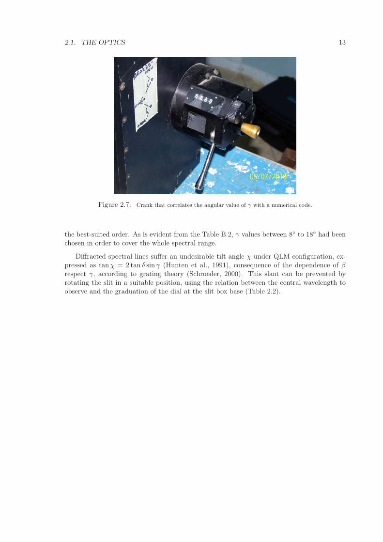
Echelle grating is ruled at 79.01 l mm−1 with a blaze angle δ of 72.◦5 (“R3.2”; tan δ = 3.2).The suitable opto-mechanical arrangement allows to adjust with high-precision the off-axisangle γ between 8◦ and 18◦, while at the same time the mirror M3 rotates and moves tofollow the central diffracted wavelength, ensuring that this wavelength will be diffracted atthe peak of the blaze function and then sent to the camera mirror M4 and the detector. Ahigh-precision external crank, placed at the right side of the spectrograph box, controls γ(from 8◦ to 18◦) correlating its angular value with a numerical code between 0000 and 7298(Fig. 2.7). Both the Echelle grating and the crank, have mechanical brakes for fixed theirmovable parts (See Fig. 2.3).

At the centre of the slit, γ = γ0 and central wavelength diffracted is (Eq. 2.1, Huntenet al. (1991)):

λ0 =2σ sin β

mcos γ0 , (2.1)

where σ = 79.01−1 mm, β is equal to the Echelle blaze angle δ of 72.◦5, and m is the best-suited dispersion order for the central wavelength selected. Appendix B presents a tablecorrelating the numerical code provided by the crank, the central wavelength displayed and

2.1. THE OPTICS 13

Figure 2.7: Crank that correlates the angular value of γ with a numerical code.

the best-suited order. As is evident from the Table B.2, γ values between 8◦ to 18◦ had beenchosen in order to cover the whole spectral range.

Diffracted spectral lines suffer an undesirable tilt angle χ under QLM configuration, ex-pressed as tanχ = 2 tan δ sin γ (Hunten et al., 1991), consequence of the dependence of βrespect γ, according to grating theory (Schroeder, 2000). This slant can be prevented byrotating the slit in a suitable position, using the relation between the central wavelength toobserve and the graduation of the dial at the slit box base (Table 2.2).


Chapter 3

Observation tutorial

The following procedure describes how to carry out an observational run with CanHiS. Asan example, we will obtain a spectrum at the highest resolution attainable at present (R ≈

140 000, with the slit as narrow as possible), using the filter named C, nominally centered at6723 Å.

3.1 Comparison lamp image

1. As a first step, we set the slit length micrometer to 0.′′200, the position micrometer to0.′′200, and the dial at slit box basis to 214.5. With this configuration the slit have aphysical length of ∼ 4.4 mm, it is centered on the optical path of the spectrograph,and it has the suitable angle for setting the spectral dispersion direction perpendicularto the spatial one. For this run, the slit width micrometer was positioned to 0.′′395;however, because of its mechanical worn-out, this is not a repeatable value.

2. Turn-on the UNe lamp by set to ON the switch placed in the aluminium case at therear side of the spectrograph (Fig. 3.1). The current intensity should reach about 25mA.

3. Rotate the handle of the entrance mirror to the INTERNAL position to select the UNelamp (Fig. 3.2), and push in the rod that moves the UNe entrance mirror until the leftedge of the box (viewed from the front) matches with the mark A in Fig. 3.3. Thisblocks the light from the telescope and ensures that the mirror will be centered on theentrance slit and will be evenly illuminated by the UNe lamp.

4. Set the upper filter wheel to the letter C (6723 Å), and the lower filter wheel to thenumber 0 (transparent BK7 window).

15

16 CHAPTER 3. OBSERVATION TUTORIAL

Figure 3.1: Electric switch for turn-on and off the UNe lamp. Ammeter is placed above the switch.

Figure 3.2: Handle for selecting the lamp or the telescope, and the rod for pushing in or out the plug thatenables the lamp or the telescope.

5. Set the Echelle grating brake and the crank brake to the OPEN position (Figure 3.4)From Table B, we choose a crank value of 5260 to center the wavelength range at

3.2. TARGET OBSERVATION 17

Figure 3.3: The mark "A" at the edge of the shelf in the guiding optic box. The left edge of the mirrorbox moved by the rod must match this mark to properly lits the entrance slit with the light from the lamp.

λc = 6707 Å (it is an intermediate value between 5270 (6710 Å) and 5360 (6705 Å) inthe 35th order. Note that the value of λc = 6707 Å is at the center of the 35th order,to avoid, as far as possible, wavelength overlap from adjacent orders.

6. Set the Echelle grating brake and the crank brake to the LOCKED position.

7. A first image of the UNe lamp can now be taken. With the narrowest slit, an exposuretime of 30 s provides clear emission lines (Fig. 3.5).

8. Once the calibration lamp image have been exposed, turn-off the UNe lamp by set toOFF the switch placed in the aluminium case at the rear side of the spectrograph.

3.2 Target observation

1. Rotate the handle of the entrance mirror to the OUT-TELESCOPE position (Fig. 3.2).

2. Pull out the rod that moves the UNe entrance mirror back to the outward limit. Thisallows the light from the telescope to enter to pass through the spectrograph entranceslit.

3. The instrument is ready to observe the target object. Fig. 3.6 shows a 1-d uncalibratedvery high-resolution (R ≈ 140 000) flux spectra of the bright G-type star (mv = 3.45)


Figure 3.4: The Echelle grating brake (above) and the crank brake (below). Echelle brake is open at theupper position and locked at the lower position. Crank brake is open at the lower position and locked at theupper position.

eta Cas, acquired with the same configuration set for the UNe lamp of Fig. 3.5, with aexposure time of 600 s. The depicted spectrum has a high signal-to-noise S/N ≥ 150.

3.2. TARGET OBSERVATION 19

Figure 3.5: Example of a 2-d and transversal cut of a spectrum from the UNe lamp. Note the saturatedNeon line at about 6717 Å.


Figure 3.6: Uncalibrated spectrum of eta Cas, acquired with CanHiS at the 2.1-m OAGH Telescope andthe 1340× 1300 CCD VersArray, 20 µ × 20 µ pixel size, during the CanHiS commissioning.

Appendix A

Normalized Filters Response

21

22 APPENDIX A. NORMALIZED FILTERS RESPONSE

Figure A.1: Normalized response for 5 intermediate band filters used by CanHiS. Dashed lines depicts theresponse of the BK7 windows, whereas dotted lines shows the response of the dimmers.

23


24 APPENDIX A. NORMALIZED FILTERS RESPONSE


Appendix B

Wavelength as Function of Crank

Number and Order

25

26APPENDIX B. WAVELENGTH AS FUNCTION OF CRANK NUMBER AND ORDER

Figure B.1: The highest orders dispersion (41 – 60) displaying their correspondign wavelengths (the bluest,from 3854 to 5832 Å) and the crank value to select a specific lambda central value λc.

27

Figure B.2: The lowest orders dispersion (21 – 59) displaying their correspondign wavelengths (the reddest,from 5756 to 11 386 Å) and the crank value to select a specific lambda central value λc.

28APPENDIX B. WAVELENGTH AS FUNCTION OF CRANK NUMBER AND ORDER

Bibliography

Hunten, D. M., Wells, W. K., Brown, R. A., Schneider, N. M., & Hilliard, R. L. 1991, , 103,1187

Schroeder, D. 2000, Astronomical Optics

Schroeder, D. J. & Hilliard, R. L. 1980, , 19, 2833

29

Documents

CanHiS User Manual Version 1 - INAOE - Pastro.inaoep.mx/portalfiles/manualCanHiS.pdf · CanHiS User Manual Version 1.1 ... 3 Observation tutorial 15 ... An external camera used as