Embed Size (px)
Citation preview
Brown Backstops versus the Green Paradox
Thomas Michielsen
Tilburg University, the Netherlands
June 6, 2011
Abstract
Imperfect climate policies may be ineffective when fossil fuel owners
respond by shifting their supply spatially (coined carbon leakage) or in-
tertemporally (the green paradox). Though these effects are usually an-
alyzed separately, the underlying mechanisms are similar. Exhaustible
fossil fuel owners must trade off present and future extraction or supply-
ing one country and the other. Whereas this is a plausible representation
for oil and natural gas, important emission-intensive substitutes such as
coal and uncoventional oil are so abundant that their owners face no such
trade-off. A decrease in coal demand in one time period or region will
therefore not trigger an equal increase in supply in the other. Moreover,
if imperfect climate policies causes oil and natural gas owners to supply
more in the near future or in countries with lax regulation, demand for
dirtier substitutes will go down. Both effects mitigate intertemporal and
spatial carbon leakage. When the substitutability between oil and coal
differs across time periods or countries, a ’strong green orthodox’ may
occur.
1 Introduction
A main challenge in combating climate change is reducing the consumption
of fossil fuels. A rapidly growing literature has recognized that policy mak-
ers should be careful when selecting appropriate instruments for bringing down
emission levels however. Climate policies typically reduce oil demand only in
some geographic areas (countries impose carbon constraints unilaterally) or in
future time periods (carbon taxes are announced ahead of implementation and
the development of clean alternatives is time-consuming). At the same time,
the supply of conventional oil and natural gas is relatively inelastic because of
1
limited reserves and low extraction costs. When faced with imperfect climate
policies, oil and natural gas owners may thus not reduce supply but merely shift
it spatially or intertemporally. Though these two channels have been named dif-
ferently in the literature (carbon leakage and the green paradox, respectively)
and are often analyzed separaretely, the mechanisms behind them are very sim-
ilar.
When only some countries reduce their emissions, pollution might move
to other countries. This ’carbon leakage’ occurs through two channels [Felder
and Rutherford, 1993]. Firstly, dirty industries move to countries with laxer
regulation. Secondly, the stringent environmental policy in adopting countries
causes the price of fossil fuels to fall, increasing their use in non-adopting re-
gions. Several papers have attempted to estimate the magnitude of this car-
bon leakage with computable general equilibrium (CGE) models [Burniaux and
Oliveira Martins, 2000, Paltsev, 2001, Babiker, 2005]. The reported leakage
rates range from a modest 2-5% to over 100% (the latter implying that uni-
lateral carbon-reduction policies actually increase global emissions). Similar
effects are found in studies on international environmental agreements: when
one group of countries jointly reduce their emissions, non-conforming countries
will free ride on their efforts and pollute more [Barrett, 1994, Hoel, 1994].
Similarly, policies that reduce future dependence on fossil fuels might en-
courage exhaustible resource owners, anticipating a drop in future demand, to
bring forward the extraction of their resources. In this way, well-intended green
policies may actually increase emissions. Sinn [2008a] coined this phenomenon
the ’green paradox’. Whereas Sinn was mainly concerned with the potentially
harmful effects of increasing future carbon taxes, other authors noted a simi-
lar effect can be caused by the development of a clean backstop technology: a
carbon-free substitute for fossil fuels. Strand [2007] and Hoel [2008] show that
reducing the costs of renewable energy sources can increase the present value of
emissions damages. However, this result may vanish if the extraction costs of
the exhaustible resource decline in the remaining stock (i.e. when oil reserves
dwindle, extraction becomes increasingly costly) or when the substitute has an
upward-sloping supply curve [Gerlagh, 2011].
The sensitivity of the green paradox to different types of backstops is ex-
amined by van der Ploeg and Withagen [2009], who distinguish between cheap
and expensive and between clean and dirty backstops. The latter denote substi-
tutes for oil and natural gas that have higher emission intensities, most notably
coal and oil from tar sands. They find that the green paradox occurs for clean
but expensive backstops (such as solar or wind), but not when the backstop is
2
sufficiently cheap relative to emissions damages, as it is then attractive to leave
part of the oil in the ground. van der Ploeg and Withagen [2011] show that
rising carbon taxes may not cause the green paradox when coal, rather than
renewables, is the primary alternative for oil. Moreover, it can be optimal to
subsidize renewables to just below the price of coal.
Considering dirty backstops is important from a policy perspective. Whereas
oil or natural gas reserves might be depleted in the next century under business-
as-usual consumption1, coal2 and tar sands3 are in much more abundant supply.
At the same time, these energy sources are very carbon-intensive. Per unit of
energy, they emit approximately 1.3-1.4 (1.8-2 if processed into synthetic fuels
[Marland, 1983]) and 1.17 [Charpentier et al., 2009] times as many greenhouse
gases as petroleum respectively. To keep global warming within tolerable lim-
its, it is therefore not only important to reduce or delay oil and natural gas
extraction, but also to ensure they are not replaced with dirty alternatives.
We seek to contribute to the literature in a number of ways. We develop a
framework that allows the analysis of both carbon leakage and the green para-
dox: two phenomena that are usually studied separately even though they are
very similar. We define leakage as the shift in emissions from the future to the
present or from conforming to non-conforming countries. The difference be-
tween intertemporal and spatial leakage is the presence or absence of a discount
rate. We show that the presence of an abundant dirty backstop reduces spatial
and intertemporal carbon leakage directly and indirectly, and can even cause
negative leakage rates.
By virtue of the abundance of their resource, owners of dirty backstops do
not need to trade off present and future extraction or supplying one country
and the other. When faced with a demand reduction in the future or in a
group of climate-conscious countries, they will thus not shift their supply to
the present or to countries with lax regulation. When exhaustible resource
emissions ’leak’ away to the present or to non-conforming countries, the resulting
leakage is mitigated indirectly because the increased exhaustible resource supply
reduces demand for the dirty backstop. Imperfect climate policies can even
reduce emissions in both time periods or both countries. Carbon taxes may
cause negative leakage rates when the substitutability between the exhaustible
1According to the 2010 BP Statistical Review of World Energy, at 2009 consumption rates
proved reserves for oil and natural gas will be exhausted in 2052 and 2073 respectively2Proved coal reserves will last until 2260 at current consumption (BP)3Reserves in Alberta alone are estimated at 1700 trln barrels (Source: Alberta’s Energy
Outlook 2009 and Supply/Demand Outlook 2010-2019)
3
resource and the dirty backstop differs between time periods or countries. We
may also call this a ’strong green orthodox’ [Grafton et al., 2010]. Developing a
clean backstop can reduce present emissions when the exhaustible resource and
the dirty backstop are good substitutes and if the emission-intensity of the dirty
backstop is high.
This paper is organized as follows. In section 2 we outline the model.
We consider a dirty exhaustible resource, an even dirtier backstop and a clean
backstop; for ease of interpretation, we sometimes refer to these as energy types.
We allow for a general substitutability structure between energy types. The
model is extended to two-period and two-country settings. In section 3 we
analyze intertemporal and spatial leakage when carbon emissions are taxed in
the future (in the two-period model) or in one country (in the two-country
model). The interplay between demand for the exhaustible resource and the
dirty backstop reduces carbon leakage. Interestingly, a future carbon tax may
cause exhaustible resource owners to delay rather than speed up extraction,
and a unilateral carbon tax may reduce welfare in other countries. In section 4,
we evaluate the impact of a cheaper clean backstop in the future. We obtain
stricter conditions for the green paradox than models that do not include the
interplay between exhaustible resource and dirty backstop demand. The models
are calibrated with interfuel elasticity estimates from previous work. Section 5
concludes. All proofs are relegated to the Appendix.
2 Model
Consider a model with three types of energy: an exhaustible resource (oil or
natural gas), a dirty backstop (coal or unconventional oil) and a clean backstop
(solar or wind power). The backstops are inexhaustible, supplied competitively
and have constant marginal costs4. The exhaustible resource is supplied com-
petitively by a group of energy-exporters and costless to extract. We assume
that for the energy-exporters, it is always optimal to fully exhaust the fossil
resource stock S5. An energy-importing country derives utility from consum-
ing energy. Energy consumption of each type is subject to decreasing marginal
utility and types are imperfect substitutes. Denote the exhaustible resource,
the dirty and the clean backstop with superscripts F , Z and C respectively.
4An upward-sloping supply curve for the clean backstop reduces intertemporal leakage [Ger-
lagh, 2011].5Relaxing this assumption makes the intertemporal leakage less severe [van der Ploeg and
Withagen, 2009, Fischer and Salant, 2010].
4
Demand functions are given by
Di(pi, p−i), i ∈ {F,Z,C} (1)
Letting qF denote the equilibrium quantity of the exhaustible resource, its in-
verse demand function is
pF = ψ(qF , pZ , pC) (2)
where for future reference we note that
∂ψ(qF , pZ , pC)
∂qF=
1∂DF
∂pF
(3)
and
∂ψ(qF , pZ , pC)
∂pi= −
∂DF
∂pi
∂DF
∂pF
, i ∈ {Z,C} (4)
∂Di
∂pi< 0, (A.1)
Energy types are imperfect substitutes for one another: demand for each type
is increasing in the price of other types (A.2) and own-price effects are stronger
than cross-price effects (A.3). We also assume that cross-price effects are sym-
metric (A.4).∂Di
∂pj> 0 (A.2)∣∣∣∣∂Di
∂pi
∣∣∣∣ > ∣∣∣∣∂Di
∂pj
∣∣∣∣ (A.3)
∂Di
∂pj=∂Dj
∂pi(A.4)
We show in Appendix A.1 that (A.4) holds if we can rewrite the demand
structure as demand for a composite good that is produced from F , Z and C
according to a homogeneous function6. This is satisfied for example by CES
demand functions.
In the main text, we will use elasticities ηij of demand for type i with respect
to the price of type j:∂Di
∂pjpj
qi= ηij
6Some energy carriers are also used to produce other goods (e.g. plastics from petroleum).
This can be reconciled with assumption (A.4) if the production function of the other good is
homogeneous of the same degree as that of the composite good.
5
Consumption of the exhaustible resource and the dirty backstop generates a
constant amount of emissions. We assume that the dirty backstop is more
emission-intensive than the exhaustible resource
E = ζF qF + ζZDZ , 0 < ζF < ζZ
We will extend the model in the time (section 2.1) and space (section 2.2)
dimension.
2.1 Intertemporal Leakage
In the sections on intertemporal carbon leakage, we append the model to include
a second time period. Denote time by subscript t, t ∈ {1, 2}. Exhaustible
resource owners discount future revenues at rate r and must decide on the
intertemporal extraction pattern. In equilibrium, they are indifferent between
extracting now and in the future
pF1 =1
1 + rpF2 (5)
Let qF1 denote period 1 exhaustible resource extraction. Substituting the stock
constraint, the indifference condition (5) reads
ψ1(qF1 , pZ , pC1 ) =
1
1 + rψ2(S − qF1 , pZ , pC2 ) (6)
We allow for emissions in the first period to be more harmful than emissions in
the second period, so that total emission damages are
Σ = E1 + βE2, β ≤ 1 (7)
When only cumulative emissions matter, β is equal to one. When society and
ecology can adapt more easily to slow rather than rapid temperature increases
[Hoel and Kverndokk, 1996, Gerlagh, 2011], a higher weight should be put on
near-term emissions (β < 1). The green paradox entails a positive relation
between the future climate policy θ2 and emissions [Sinn, 2008b]. Following
Gerlagh [2011], we differentiate between a weak green paradox (the future cli-
mate policy increases present emissions) and a strong green paradox (emission
damages increase).
Definition 1. The weak green paradox occurs if
∂E1
∂θ2> 0
6
The strong green paradox occurs if
∂Σ
∂θ2> 0
Analogous to the literature on (spatial) carbon leakage, we define the in-
tertemporal carbon leakage of a future climate policy as the share of period 2
emission reductions that ’leaks’ away to the first period.
Definition 2. The intertemporal leakage β∗t of second-period policy θ2 is the
increase in period 1 emissions over the decrease in period 2 emissions.
β∗t = −
∂E1
∂θ2∂E2
∂θ2
Both green paradoxes can be related to the intertemporal leakage rate β∗t
in a straightforward way. As intertemporal leakage is positive if and only if
the future carbon tax increases present emissions, the weak green paradox is
equivalent to β∗t > 0. The strong green paradox occurs if the leakage rate exceeds
the emission discount rate (β∗t > β). We will employ the following shorthand
notation: Dit = Di
t
(pit, p
−it
), ψ1 = ψ1(qF1 , p
Z , pC1 ), ψ2 = ψ2(S − qF1 , pZ , pC2 ).
2.2 Spatial Leakage
For analyzing spatial leakage, we consider two countries. Denote a conforming
country with subscript A and a non-conforming country with subscript B. The
countries are of the same size, have identical demand functions and differ only
with respect to climate policy. The price of the exhaustible resource must be
equal in both countries
pFA = pFB
Letting qFA denote the equilibrium quantity of the exhaustible resource consumed
in country A, this translates into a condition identical to (6) except for the
absence of a discount rate
ψ(qFA , pZ , pC) = ψ(S − qFA , pZ , pC)
Emission damages are equal to the unweighted sum of emissions
Ξ = EA + EB
Definition 3. Spatial carbon leakage β∗s of unilateral policy θA is the increase
in emissions in country B over the emission reduction in country A
β∗s = −
∂E1
∂θA∂E2
∂θA
7
Total emissions go down when β∗s < 1. When β∗
s < 0, the unilateral policy
decreases emissions in both countries.
We will discuss carbon taxes (section 3) and investment in green technologies
(section 4) in turn, differentiating between intertemporal and spatial carbon
leakage. In both sections, our focus will be on the impact of (stricter) climate
policies on emissions through the pattern of exhaustible resource extraction and
changes in the level of dirty backstop use.
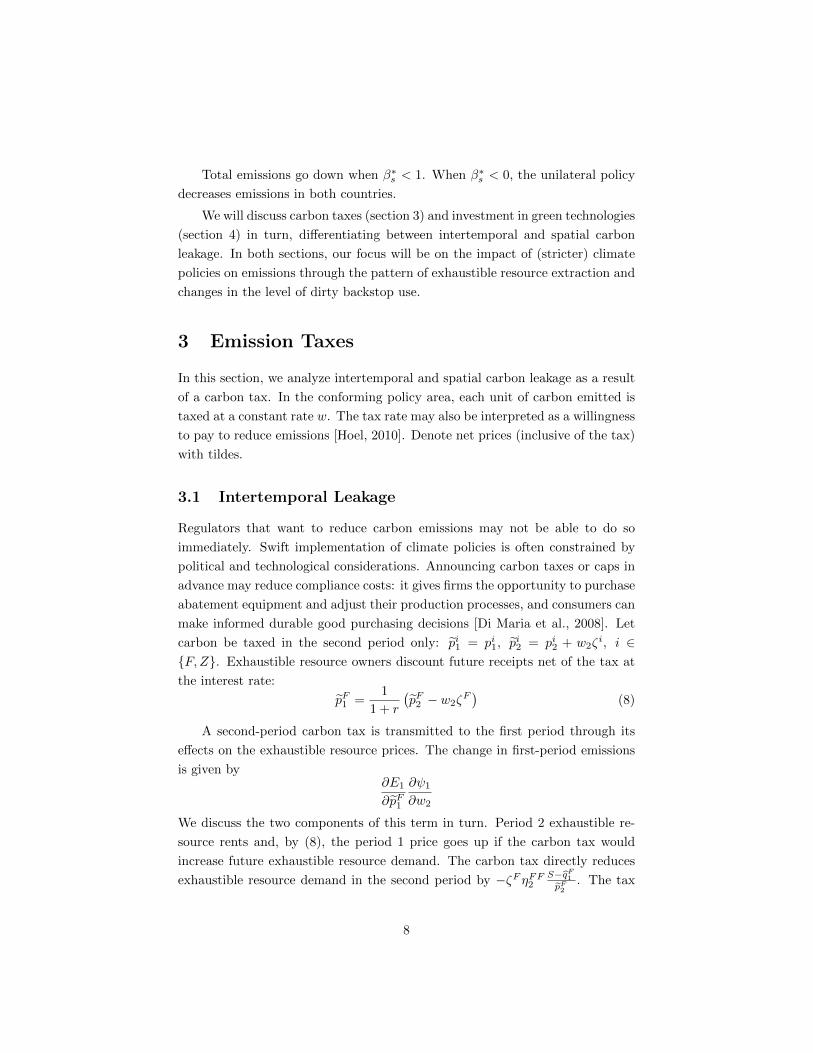
3 Emission Taxes
In this section, we analyze intertemporal and spatial carbon leakage as a result
of a carbon tax. In the conforming policy area, each unit of carbon emitted is
taxed at a constant rate w. The tax rate may also be interpreted as a willingness
to pay to reduce emissions [Hoel, 2010]. Denote net prices (inclusive of the tax)
with tildes.
3.1 Intertemporal Leakage
Regulators that want to reduce carbon emissions may not be able to do so
immediately. Swift implementation of climate policies is often constrained by
political and technological considerations. Announcing carbon taxes or caps in
advance may reduce compliance costs: it gives firms the opportunity to purchase
abatement equipment and adjust their production processes, and consumers can
make informed durable good purchasing decisions [Di Maria et al., 2008]. Let
carbon be taxed in the second period only: pi1 = pi1, pi2 = pi2 + w2ζ
i, i ∈{F,Z}. Exhaustible resource owners discount future receipts net of the tax at
the interest rate:
pF1 =1
1 + r
(pF2 − w2ζ
F)
(8)
A second-period carbon tax is transmitted to the first period through its
effects on the exhaustible resource prices. The change in first-period emissions
is given by∂E1
∂pF1
∂ψ1
∂w2
We discuss the two components of this term in turn. Period 2 exhaustible re-
source rents and, by (8), the period 1 price goes up if the carbon tax would
increase future exhaustible resource demand. The carbon tax directly reduces
exhaustible resource demand in the second period by −ζF ηFF2S−qF1pF2
. The tax
8
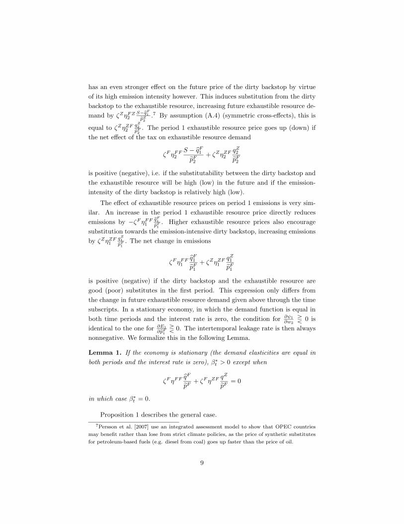
has an even stronger effect on the future price of the dirty backstop by virtue
of its high emission intensity however. This induces substitution from the dirty
backstop to the exhaustible resource, increasing future exhaustible resource de-
mand by ζZηFZ2S−qF1pZ2
.7 By assumption (A.4) (symmetric cross-effects), this is
equal to ζZηZF2qZ2pF2
. The period 1 exhaustible resource price goes up (down) if
the net effect of the tax on exhaustible resource demand
ζF ηFF2
S − qF1pF2
+ ζZηZF2
qZ2pF2
is positive (negative), i.e. if the substitutability between the dirty backstop and
the exhaustible resource will be high (low) in the future and if the emission-
intensity of the dirty backstop is relatively high (low).
The effect of exhaustible resource prices on period 1 emissions is very sim-
ilar. An increase in the period 1 exhaustible resource price directly reduces
emissions by −ζF ηFF1qF1pF1
. Higher exhaustible resource prices also encourage
substitution towards the emission-intensive dirty backstop, increasing emissions
by ζZηZF1qZ1pF1
. The net change in emissions
ζF ηFF1
qF1pF1
+ ζZηZF1
qZ1pF1
is positive (negative) if the dirty backstop and the exhaustible resource are
good (poor) substitutes in the first period. This expression only differs from
the change in future exhaustible resource demand given above through the time
subscripts. In a stationary economy, in which the demand function is equal in
both time periods and the interest rate is zero, the condition for ∂ψ1
∂w2R 0 is
identical to the one for ∂E1
∂pF1R 0. The intertemporal leakage rate is then always
nonnegative. We formalize this in the following Lemma.
Lemma 1. If the economy is stationary (the demand elasticities are equal in
both periods and the interest rate is zero), β∗t > 0 except when
ζF ηFFqF
pF+ ζF ηZF
qZ
pF= 0
in which case β∗t = 0.
Proposition 1 describes the general case.
7Persson et al. [2007] use an integrated assessment model to show that OPEC countries
may benefit rather than lose from strict climate policies, as the price of synthetic substitutes
for petroleum-based fuels (e.g. diesel from coal) goes up faster than the price of oil.
9
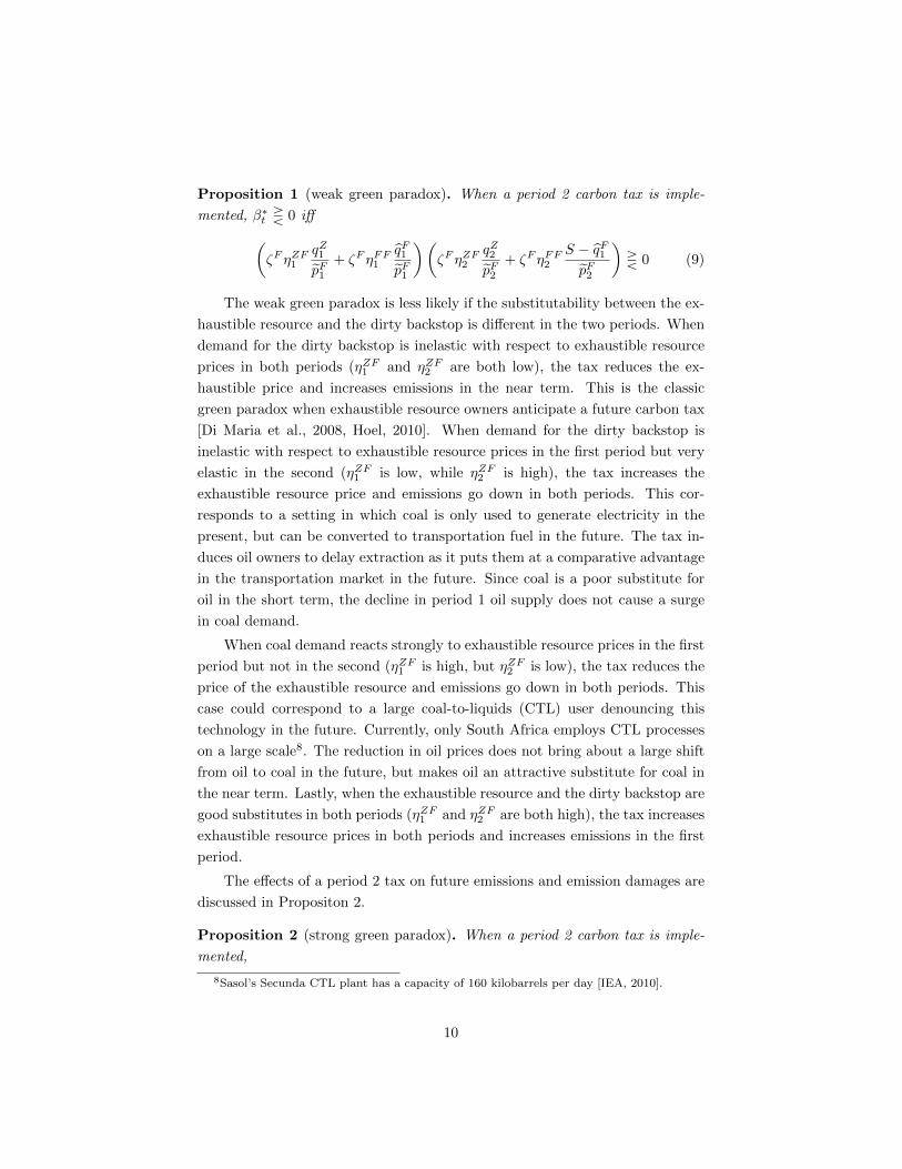
Proposition 1 (weak green paradox). When a period 2 carbon tax is imple-
mented, β∗t R 0 iff(ζF ηZF1
qZ1pF1
+ ζF ηFF1
qF1pF1
)(ζF ηZF2
qZ2pF2
+ ζF ηFF2
S − qF1pF2
)R 0 (9)
The weak green paradox is less likely if the substitutability between the ex-
haustible resource and the dirty backstop is different in the two periods. When
demand for the dirty backstop is inelastic with respect to exhaustible resource
prices in both periods (ηZF1 and ηZF2 are both low), the tax reduces the ex-
haustible price and increases emissions in the near term. This is the classic
green paradox when exhaustible resource owners anticipate a future carbon tax
[Di Maria et al., 2008, Hoel, 2010]. When demand for the dirty backstop is
inelastic with respect to exhaustible resource prices in the first period but very
elastic in the second (ηZF1 is low, while ηZF2 is high), the tax increases the
exhaustible resource price and emissions go down in both periods. This cor-
responds to a setting in which coal is only used to generate electricity in the
present, but can be converted to transportation fuel in the future. The tax in-
duces oil owners to delay extraction as it puts them at a comparative advantage
in the transportation market in the future. Since coal is a poor substitute for
oil in the short term, the decline in period 1 oil supply does not cause a surge
in coal demand.
When coal demand reacts strongly to exhaustible resource prices in the first
period but not in the second (ηZF1 is high, but ηZF2 is low), the tax reduces the
price of the exhaustible resource and emissions go down in both periods. This
case could correspond to a large coal-to-liquids (CTL) user denouncing this
technology in the future. Currently, only South Africa employs CTL processes
on a large scale8. The reduction in oil prices does not bring about a large shift
from oil to coal in the future, but makes oil an attractive substitute for coal in
the near term. Lastly, when the exhaustible resource and the dirty backstop are
good substitutes in both periods (ηZF1 and ηZF2 are both high), the tax increases
exhaustible resource prices in both periods and increases emissions in the first
period.
The effects of a period 2 tax on future emissions and emission damages are
discussed in Propositon 2.
Proposition 2 (strong green paradox). When a period 2 carbon tax is imple-
mented,
8Sasol’s Secunda CTL plant has a capacity of 160 kilobarrels per day [IEA, 2010].
10
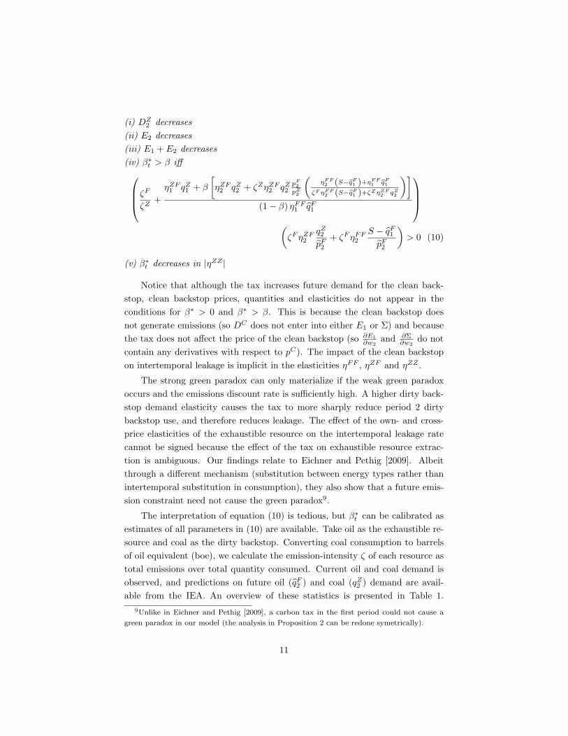
(i) DZ2 decreases
(ii) E2 decreases
(iii) E1 + E2 decreases
(iv) β∗t > β iffζFζZ +
ηZF1 qZ1 + β
[ηZF2 qZ2 + ζZηZF2 qZ2
pF2pZ2
(ηFF2 (S−qF1 )+ηFF
1 qF1
ζF ηFF2 (S−qF1 )+ζZηZF
2 qZ2
)](1− β) ηFF1 qF1
(ζF ηZF2
qZ2pF2
+ ζF ηFF2
S − qF1pF2
)> 0 (10)
(v) β∗t decreases in |ηZZ |
Notice that although the tax increases future demand for the clean back-
stop, clean backstop prices, quantities and elasticities do not appear in the
conditions for β∗ > 0 and β∗ > β. This is because the clean backstop does
not generate emissions (so DC does not enter into either E1 or Σ) and because
the tax does not affect the price of the clean backstop (so ∂E1
∂w2and ∂Σ
∂w2do not
contain any derivatives with respect to pC). The impact of the clean backstop
on intertemporal leakage is implicit in the elasticities ηFF , ηZF and ηZZ .
The strong green paradox can only materialize if the weak green paradox
occurs and the emissions discount rate is sufficiently high. A higher dirty back-
stop demand elasticity causes the tax to more sharply reduce period 2 dirty
backstop use, and therefore reduces leakage. The effect of the own- and cross-
price elasticities of the exhaustible resource on the intertemporal leakage rate
cannot be signed because the effect of the tax on exhaustible resource extrac-
tion is ambiguous. Our findings relate to Eichner and Pethig [2009]. Albeit
through a different mechanism (substitution between energy types rather than
intertemporal substitution in consumption), they also show that a future emis-
sion constraint need not cause the green paradox9.
The interpretation of equation (10) is tedious, but β∗t can be calibrated as
estimates of all parameters in (10) are available. Take oil as the exhaustible re-
source and coal as the dirty backstop. Converting coal consumption to barrels
of oil equivalent (boe), we calculate the emission-intensity ζ of each resource as
total emissions over total quantity consumed. Current oil and coal demand is
observed, and predictions on future oil (qF2 ) and coal (qZ2 ) demand are avail-
able from the IEA. An overview of these statistics is presented in Table 1.
9Unlike in Eichner and Pethig [2009], a carbon tax in the first period could not cause a
green paradox in our model (the analysis in Proposition 2 can be redone symetrically).
11
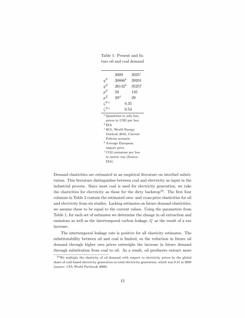
Table 1: Present and fu-
ture oil and coal demand
2009 2035c
qF 30806b 39201
qZ 26142b 35257
pF 59 135
pZ 29d 29
ζF e 0.35
ζZe 0.54
a Quantities in mln boe,
prices in USD per boeb EIAc IEA, World Energy
Outlook 2010, Current
Policies scenariod Average European
import pricee CO2 emissions per boe
in metric ton (Source:
EIA)
Demand elasticities are estimated in an empirical literature on interfuel substi-
tution. This literature distinguishes between coal and electricity as input in the
industrial process. Since most coal is used for electricity generation, we take
the elasticities for electricity as those for the dirty backstop10. The first four
columns in Table 2 contain the estimated own- and cross-price elasticities for oil
and electricity from six studies. Lacking estimates on future demand elasticities,
we assume these to be equal to the current values. Using the parameters from
Table 1, for each set of estimates we determine the change in oil extraction and
emissions as well as the intertemporal carbon leakage β∗t as the result of a tax
increase.
The intertemporal leakage rate is positive for all elasticity estimates. The
substitutability between oil and coal is limited, so the reduction in future oil
demand through higher own prices outweighs the increase in future demand
through substitution from coal to oil. As a result, oil producers extract more
10We multiply the elasticity of oil demand with respect to electricity prices by the global
share of coal-based electricity generation in total electricity generation, which was 0.41 in 2008
(source: CIA World Factbook 2009)
12
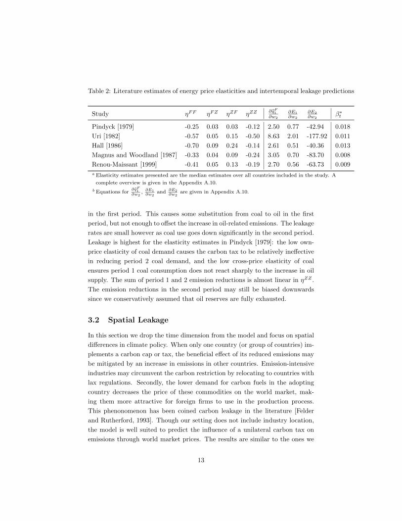
Table 2: Literature estimates of energy price elasticities and intertemporal leakage predictions
Study ηFF ηFZ ηZF ηZZ∂qF1∂w2
∂E1
∂w2
∂E2
∂w2β∗t
Pindyck [1979] -0.25 0.03 0.03 -0.12 2.50 0.77 -42.94 0.018
Uri [1982] -0.57 0.05 0.15 -0.50 8.63 2.01 -177.92 0.011
Hall [1986] -0.70 0.09 0.24 -0.14 2.61 0.51 -40.36 0.013
Magnus and Woodland [1987] -0.33 0.04 0.09 -0.24 3.05 0.70 -83.70 0.008
Renou-Maissant [1999] -0.41 0.05 0.13 -0.19 2.70 0.56 -63.73 0.009
a Elasticity estimates presented are the median estimates over all countries included in the study. A
complete overview is given in the Appendix A.10.
b Equations for∂qF1∂w2
, ∂E1∂w2
and ∂E2∂w2
are given in Appendix A.10.
in the first period. This causes some substitution from coal to oil in the first
period, but not enough to offset the increase in oil-related emissions. The leakage
rates are small however as coal use goes down significantly in the second period.
Leakage is highest for the elasticity estimates in Pindyck [1979]: the low own-
price elasticity of coal demand causes the carbon tax to be relatively ineffective
in reducing period 2 coal demand, and the low cross-price elasticity of coal
ensures period 1 coal consumption does not react sharply to the increase in oil
supply. The sum of period 1 and 2 emission reductions is almost linear in ηZZ .
The emission reductions in the second period may still be biased downwards
since we conservatively assumed that oil reserves are fully exhausted.
3.2 Spatial Leakage
In this section we drop the time dimension from the model and focus on spatial
differences in climate policy. When only one country (or group of countries) im-
plements a carbon cap or tax, the beneficial effect of its reduced emissions may
be mitigated by an increase in emissions in other countries. Emission-intensive
industries may circumvent the carbon restriction by relocating to countries with
lax regulations. Secondly, the lower demand for carbon fuels in the adopting
country decreases the price of these commodities on the world market, mak-
ing them more attractive for foreign firms to use in the production process.
This phenonomenon has been coined carbon leakage in the literature [Felder
and Rutherford, 1993]. Though our setting does not include industry location,
the model is well suited to predict the influence of a unilateral carbon tax on
emissions through world market prices. The results are similar to the ones we
13
obtained when the carbon tax is implemented only in the future. A carbon
tax in one country need not increase emissions in non-adopting countries. We
calibrate a simple demand structure and find that the world market price effect
causes only very modest carbon leakage. Our results suggest that high leakage
rates as in Babiker [2005] require very large industry relocation effects.
Proposition 3. When country A implements a carbon tax unilaterally,
(i) β∗s R 0 iff(
ζZηZF1
qZBpFB
+ ζZηFFBqFBpFB
)(ζF ηZF2
qZApFA
+ ζF ηFFAS − qFBpFA
)R 0 (11)
(ii) β∗s < 1
The carbon tax in country A reduces total emissions Ξ. The conditions for
a negative spatial leakage rate are analogous to those for negative intertemporal
leakage in section 3.1. The second term in brackets is positive (negative) when
the unilateral tax increases (decreases) exhaustible resource demand in country
A. The first term determines whether emissions in country B increase (positive)
or decrease (negative) in the exhaustible resource price. Carbon leakage can be
negative when the substitutability between the exhaustible resource and the
dirty backstop differs across countries. Notice that if the tax causes an increase
in exhaustible resource demand in country A (i.e. when the second term is
positive), country B is made worse off by country A’s climate policy.
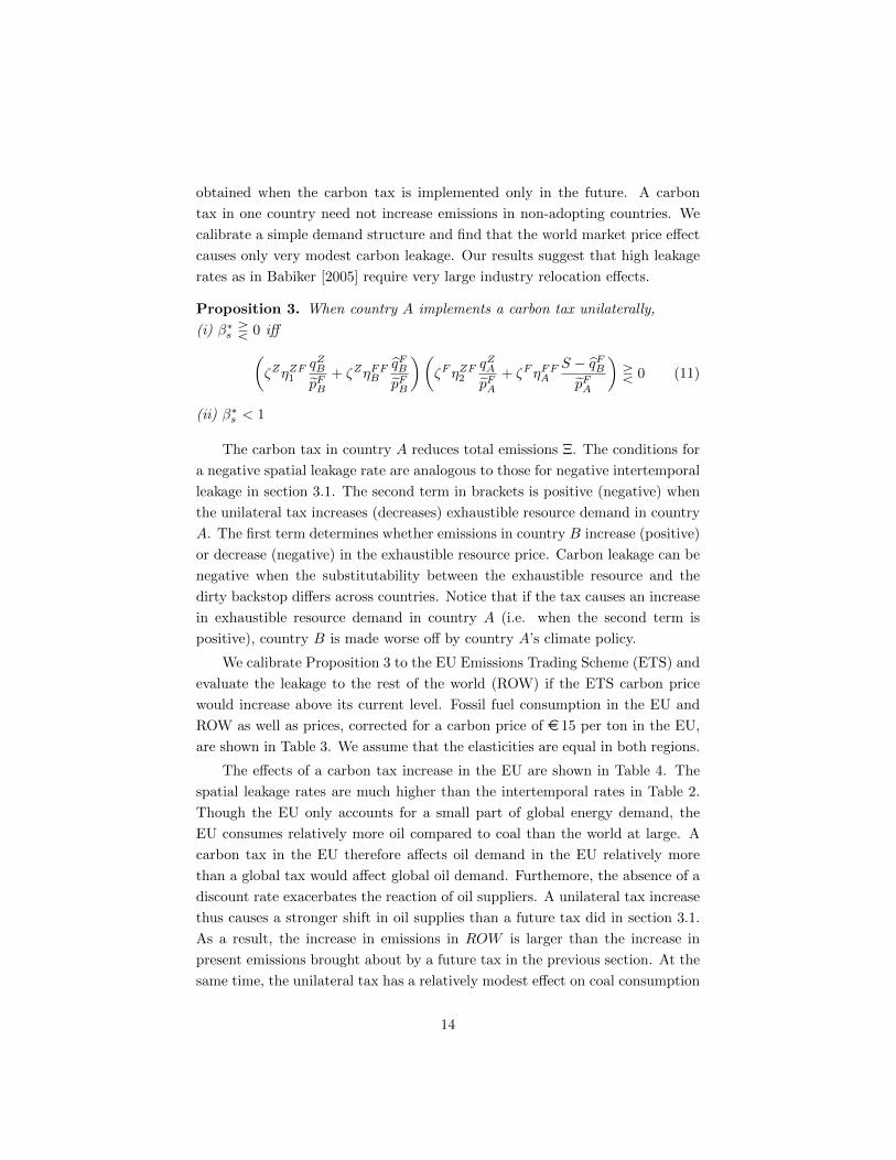
We calibrate Proposition 3 to the EU Emissions Trading Scheme (ETS) and
evaluate the leakage to the rest of the world (ROW) if the ETS carbon price
would increase above its current level. Fossil fuel consumption in the EU and
ROW as well as prices, corrected for a carbon price of e 15 per ton in the EU,
are shown in Table 3. We assume that the elasticities are equal in both regions.
The effects of a carbon tax increase in the EU are shown in Table 4. The
spatial leakage rates are much higher than the intertemporal rates in Table 2.
Though the EU only accounts for a small part of global energy demand, the
EU consumes relatively more oil compared to coal than the world at large. A
carbon tax in the EU therefore affects oil demand in the EU relatively more
than a global tax would affect global oil demand. Furthemore, the absence of a
discount rate exacerbates the reaction of oil suppliers. A unilateral tax increase
thus causes a stronger shift in oil supplies than a future tax did in section 3.1.
As a result, the increase in emissions in ROW is larger than the increase in
present emissions brought about by a future tax in the previous section. At the
same time, the unilateral tax has a relatively modest effect on coal consumption
14
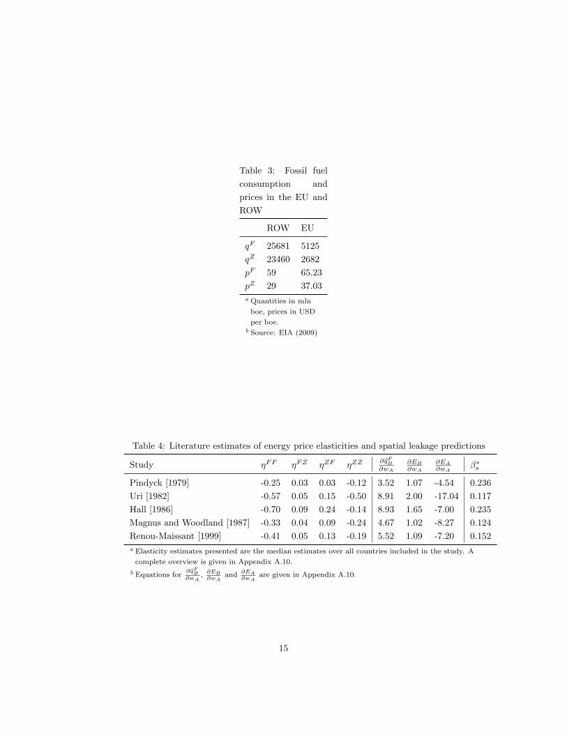
Table 3: Fossil fuel
consumption and
prices in the EU and
ROW
ROW EU
qF 25681 5125
qZ 23460 2682
pF 59 65.23
pZ 29 37.03
a Quantities in mln
boe, prices in USD
per boe.b Source: EIA (2009)
Table 4: Literature estimates of energy price elasticities and spatial leakage predictions
Study ηFF ηFZ ηZF ηZZ∂qFB∂wA
∂EB
∂wA
∂EA
∂wAβ∗s
Pindyck [1979] -0.25 0.03 0.03 -0.12 3.52 1.07 -4.54 0.236
Uri [1982] -0.57 0.05 0.15 -0.50 8.91 2.00 -17.04 0.117
Hall [1986] -0.70 0.09 0.24 -0.14 8.93 1.65 -7.00 0.235
Magnus and Woodland [1987] -0.33 0.04 0.09 -0.24 4.67 1.02 -8.27 0.124
Renou-Maissant [1999] -0.41 0.05 0.13 -0.19 5.52 1.09 -7.20 0.152
a Elasticity estimates presented are the median estimates over all countries included in the study. A
complete overview is given in Appendix A.10.
b Equations for∂qFB∂wA
, ∂EB∂wA
and ∂EA∂wA
are given in Appendix A.10.
15
in the EU as coal demand is already very low to begin with. These two forces
contrive to cause higher spatial leakage rates. The ordering of leakage rates is
similar to that of the intertemporal rates. Leakage is lower when coal demand
is more elastic (as the tax then decreases coal demand more strongly in the
EU) and when the cross-elasticities of oil and coal are large compared to the
own-price elasticity of oil (this decreases the shift in oil supply to ROW and
amplifies the drop in coal demand in ROW , respectively).
The leakage rates in Table 4 are much smaller than some estimates reported
in the CGE literature on carbon leakage. Babiker [2005], who finds leakage rates
up to 130%, claims that most CGE models do not model industry location
correctly and thus underestimate the leakage rate. Our model does not include
production, but it can be argued that industry location is implicit in the demand
function. Other authors are of the opinion that the energy price channel is the
most important determinant of carbon leakage [Paltsev, 2001, Fischer and Fox,
2009, Kuik and Hofkes, 2010].
4 A Cheaper Clean Backstop
Instead of implementing a carbon tax, climate-conscious countries may opt to
reduce emissions by stimulating the development of clean alternatives to fossil
fuels. Such investments have strong public good characteristics: once a break-
through has been achieved in one country, the technology quickly becomes avail-
able in other countries [Golombek and Hoel, 2004, Gerlagh and Kuik]. As tech-
nology differences for renewable energy sources between countries are likely to
be limited, we restrict ourselves to intertemporal carbon leakage in this section.
4.1 Intertemporal Leakage
Developing alternative energy sources requires resources to be committed well
before new technologies can be put to use. The cost of the clean backstop
is lower in the second period: pC2 ≤ pC1 . The cost of the dirty backstop is
assumed to remain constant over time, so the time subscript for pZ is omitted.
We are interested in the effect of a reduction in pC2 on emissions. A lower pC2decreases the right hand side of (6). For exhaustible resource owners to remain
indifferent between extracting in either period, period 1 extraction qF1 must go
up. This is the classic green paradox result [Strand, 2007, Hoel, 2008]. In the
next Propositions, we show how the occurence of the weak and the strong green
paradox depend on the emission intensities and the substitutability structure.
16
Proposition 4 (weak green paradox). When the clean backstop becomes cheaper
in period 2, β∗t > 0 iff
ζF ηFF1
qF1pF1
+ ζZηZF1
qZ1pF1
< 0 (12)
As opposed to the implementation of a future carbon tax, exhaustible re-
source owners always bring extraction forward when clean alternatives become
cheaper in the future. The lower period 1 exhaustible resource price also causes a
drop in demand for the emission-intensive dirty backstop however. Both of these
effects are proportional to the change in period 1 exhaustible resource extrac-
tion∂qF1∂pC2
. Because period 2 parameters only affect period 1 emissions through
this term, the condition for the weak green paradox solely consists of period 1
parameters. The occurence of the weak green paradox hinges on whether the in-
crease in exhaustible resource-related emissions outweighs the decrease in dirty
backstop-related emissions (12). This is more likely if the relative emission-
intensity of the exhaustible resource is high (this puts a higher weight on the
increase in exhaustible resource demand vis a vis the drop in demand for the
dirty backstop) and if the substitutability between the exhaustible resource and
the dirty backstop is low (this dampens the response of dirty backstop demand
to the drop in exhaustible resource prices).
In order to facilitate calibrations, we may rewrite the condition for the weak
green paradox asζF
ζZ>
ηZF1
−ηFF1
qZ1qF1
In Table 1, we saw that ζF
ζZ= 0.65 and
qZ1qF1
= 0.91. Intertemporal leakage is
thus positive for ηZF
−ηFF < 0.72. The elasticity ratio is considerably smaller than
0.72 for all studies in Tables 2 and 4, so the development of clean technologies
is likely to bring about the weak green paradox.
Proposition 5 (strong green paradox). When the clean backstop becomes cheaper
in period 2,
(i) β∗t > β iff
ζF
ζZ>ηZF1 qZ1 + β
[ηZF2 qZ2 +
ηZC2
ηFC2
qZ2S−qF1
(−ηFF2
(S − qF1
)− ηFF1 qF1
)](1− β)
(−ηFF1
)qF1
(13)
(ii) β∗t increases in ηFC and |ηFF |
(iii) β∗t decreases in ηZF and ηZC
17
The technological advance reduces the price of the exhaustible resource in
both periods: the indifference requirement (5) mandates that the price drop in
period 1 (brought about by increased supply) is accompanied by a proportional
decrease in period 2. Together with the lower period 2 clean backstop prices,
this reduces demand for the dirty backstop in both periods. This means that
the strong green paradox can only arise if the lower pC2 causes a sufficiently
large shift in the extraction pattern of the exhaustible resource, so that the
damage from bringing forward exhaustible resource emissions (the denominator
in (13)) exceeds the benefits of reduced dirty backstop consumption in both
periods (the two terms in the numerator). Intertemporal leakage decreases in
ηZF and ηZC (as the technology advance then induces more substitution away
from the dirty backstop). When ηFC is high, a decrease in pC2 triggers a stronger
shift in the intertemporal extraction pattern of the exhaustible resource. The
resulting price drop, which is an important determinant of substitution from
the dirty backstop to the exhaustible resource, depends negatively on the own-
price elasticity |ηFF |. Therefore, β∗t increases in ηFC and |ηFF |. We calibrate
Proposition 5 at the end of this section.
Under reasonable assumptions on the substitutability structure, we are able
to obtain more powerful results about the occurence of the green paradox, as
we will show in the next Corollaries. The energy market can be divided into a
submarket for electricity and one for transport. Natural gas (F ), coal (Z) and
wind and solar energy (C) more readily lend themselves for electricity genera-
tion, whereas oil (F ), tar sands (Z) and biofuels (C) are foremostly used in the
transportation sector. It can be argued that two energy types that are employed
in the same submarket are very close substitutes.
4.1.1 Case I: Developing Alternative Fuels
Suppose that the exhaustible resource and the clean backstop are perfect sub-
stitutes. Food-based biofuels, though not efficient enough to completely replace
petroleum-based fuels [Hill et al., 2006], enjoy significant market shares in the
US and Brazil already. Synthetic biofuels are a promising alternative in the long
run, but still require very large R&D efforts [Blok, 2006, IEA, 2010]. We are pri-
marily interested in this case as a reference point however: the assumption that
clean backstops are perfect substitutes for exhaustible fossil fuels is common in
green paradox models. It leads to the most powerful green paradox results in
the literature: when the substitutability between fossil fuel and the clean back-
stop is high, a cheaper green backstop will cause a larger exhaustible resource
18
demand drop in the future and consequently a larger increase in short-term ex-
traction. When the exhaustible resource and the green backstop are imperfect
substitutes, exhaustible resource owners are ensured of future demand for their
commodities even at higher prices, and the green paradox may vanish [Gerlagh,
2011].
Corollary 1. With perfect substitution between the exhaustible resource and the
clean backstop
(i) if pC2 > ψ2, a decrease in pC2 has no effect
(ii) if pC2 = ψ2, then β∗t > β if
ζF
ζZ>
ηZF1 qZ1 + βqZ2 ηZF2
(1− β)(−ηFF1
)qF1
(14)
The price of the exhaustible resource no longer depends on supply but
is fully determined by the period 2 clean backstop price. The numerator of
(14), which reflects the sensitivity of dirty backstop demand with respect to
exhaustible resource (and clean backstop) prices, is therefore independent of
qF1 . As in section 4, the Strong GP is less likely the higher the substitution
between the dirty backstop and the exhaustible resource, and the lower the
increase in period 1 exhaustible resource extraction as a result of lower period
2 clean backstop prices. In accordance with the literature, the condition for the
Strong GP is weaker than in the general case. In (13), the only effect that is
not proportional to the intertemporal change in exhaustible resource extraction∂qF1∂pC2
is the direct effect of lower clean backstop prices on period 2 dirty backstop
demand∂DZ
2
∂pC2, which works against the strong green paradox. Since qF1 reacts
more strongly to pC2 in this special case, the strong green paradox becomes
more likely when the exhaustible resource and the clean backstop are perfect
substitutes.
The results from Corollary 1 show that if we take into consideration the
availability of dirty backstops, the substitutability structure that is most con-
dusive to the green paradox no longer suffices for its occurence: even when the
exhaustible resource and the clean backstop are perfect substitutes, both short-
term emissions and the emission damages may go down as a result of lower clean
backstop prices.
4.1.2 Case II: Renewable Energy for Electricity
An empirically very relevant case is perfect substitutability between the clean
and dirty backstop. The opportunities to employ renewable energy are highest
19
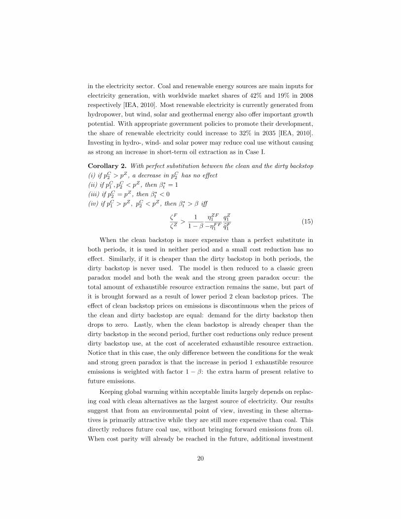
in the electricity sector. Coal and renewable energy sources are main inputs for
electricity generation, with worldwide market shares of 42% and 19% in 2008
respectively [IEA, 2010]. Most renewable electricity is currently generated from
hydropower, but wind, solar and geothermal energy also offer important growth
potential. With appropriate government policies to promote their development,
the share of renewable electricity could increase to 32% in 2035 [IEA, 2010].
Investing in hydro-, wind- and solar power may reduce coal use without causing
as strong an increase in short-term oil extraction as in Case I.
Corollary 2. With perfect substitution between the clean and the dirty backstop
(i) if pC2 > pZ , a decrease in pC2 has no effect
(ii) if pC1 , pC2 < pZ , then β∗
t = 1
(iii) if pC2 = pZ , then β∗t < 0
(iv) if pC1 > pZ , pC2 < pZ , then β∗t > β iff
ζF
ζZ>
1
1− βηZF1
−ηFF1
qZ1qF1
(15)
When the clean backstop is more expensive than a perfect substitute in
both periods, it is used in neither period and a small cost reduction has no
effect. Similarly, if it is cheaper than the dirty backstop in both periods, the
dirty backstop is never used. The model is then reduced to a classic green
paradox model and both the weak and the strong green paradox occur: the
total amount of exhaustible resource extraction remains the same, but part of
it is brought forward as a result of lower period 2 clean backstop prices. The
effect of clean backstop prices on emissions is discontinuous when the prices of
the clean and dirty backstop are equal: demand for the dirty backstop then
drops to zero. Lastly, when the clean backstop is already cheaper than the
dirty backstop in the second period, further cost reductions only reduce present
dirty backstop use, at the cost of accelerated exhaustible resource extraction.
Notice that in this case, the only difference between the conditions for the weak
and strong green paradox is that the increase in period 1 exhaustible resource
emissions is weighted with factor 1 − β: the extra harm of present relative to
future emissions.
Keeping global warming within acceptable limits largely depends on replac-
ing coal with clean alternatives as the largest source of electricity. Our results
suggest that from an environmental point of view, investing in these alterna-
tives is primarily attractive while they are still more expensive than coal. This
directly reduces future coal use, without bringing forward emissions from oil.
When cost parity will already be reached in the future, additional investment
20
does not cause a further reduction in future coal use, and only reduces present
coal use indirectly. The strong green paradox then becomes more likely. This re-
sult relates to Fischer and Salant [2010] and van der Ploeg and Withagen [2011].
Fischer and Salant [2010] analyze the effect of cheaper backstops in the presence
of high- and low-cost oil. They find that for moderate investments, the cheaper
backstop will cause the high-cost oil to remain in the ground and thus improve
the environment. Beyond that point, further investments will bring forward
the extraction of the low-cost oil and cause a ’renewed’ green paradox. van der
Ploeg and Withagen [2011] argue that it can be optimal to subsidize renewables
to just below the price of coal if global warming damages are sufficiently severe.
4.1.3 Case III: Conventional and Unconventional Oil
In this subsection, we look at the effects of cheaper renewable electricity on
the use of unconventional oil. Tar sands deposits in Canada and Venezuela are
thought to exceed reserves of conventional oil. Extracting energy from uncoven-
tional oil is relatively costly: most new oil sands projects are estimated to be
profitable at oil prices of $65-$75 per barrel [IEA, 2010]. Unconventional oil is
also more emission-intensive: producing synthetic crude oil from tar sands gen-
erates 3-4 times as many emissions as from conventional oil; as most emissions
from oil are generated during consumption however, the difference in well-to-
wheels emissions is in the order of 15-20% [Charpentier et al., 2009].
Corollary 3. With perfect substitution between the exhaustible resource and the
dirty backstop
(i) if ψ2 < pZ , both the Weak and the strong green paradox occur
(ii) if ψ2 = pZ , neither the Weak nor the strong green paradox occurs
The environmental implications of investment in the green backstop are
similar as in subsection 4.1.2. If the economy is under regime (ii), cost reductions
will initally benefit the environment by reducing the use of the dirty backstop in
period 2, without affecting the pattern of exhaustible resource extraction. At a
certain point however, demand for the dirty backstop in period 2 will go to zero
and the economy moves into regime (i), in which additional investment only
brings forward the extraction of the exhaustible resource and the green paradox
returns.
21
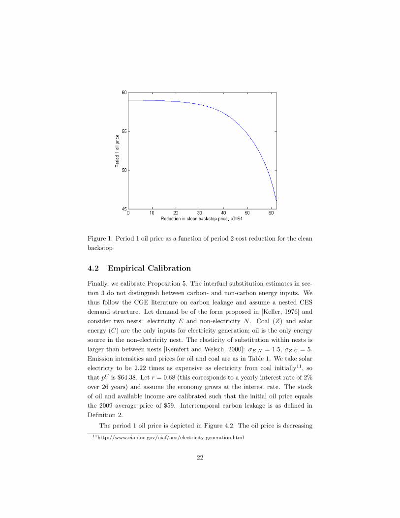
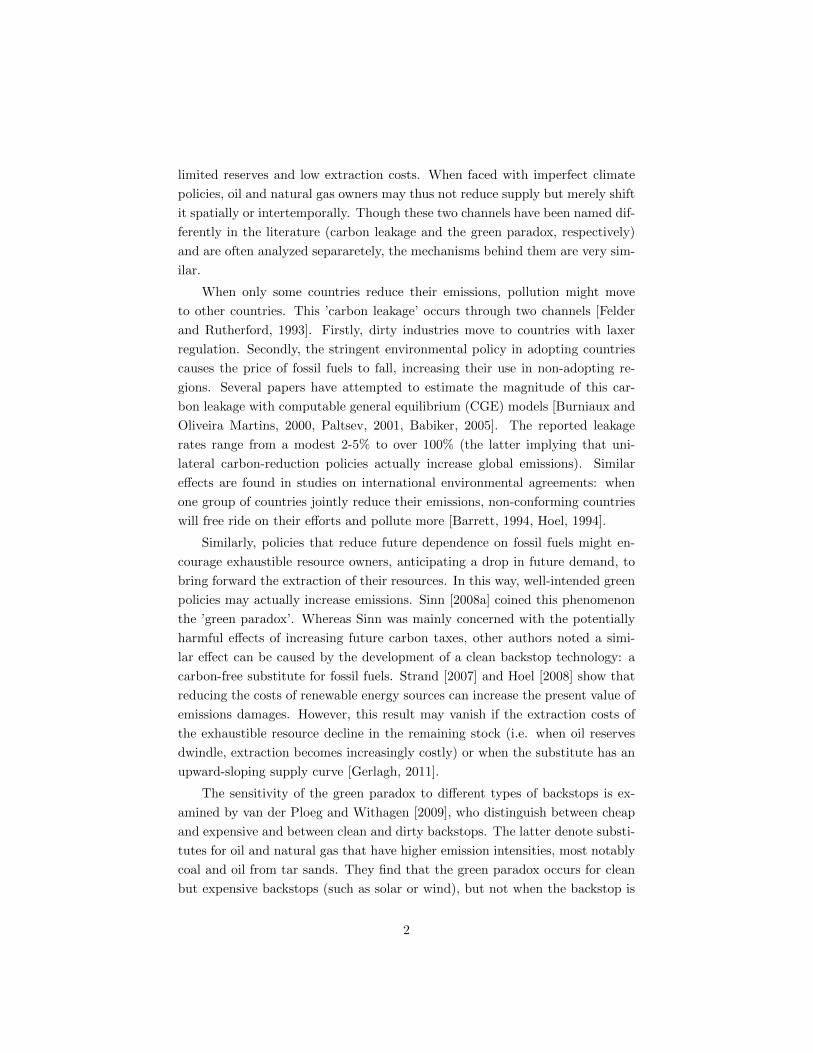
Figure 1: Period 1 oil price as a function of period 2 cost reduction for the clean
backstop
4.2 Empirical Calibration
Finally, we calibrate Proposition 5. The interfuel substitution estimates in sec-
tion 3 do not distinguish between carbon- and non-carbon energy inputs. We
thus follow the CGE literature on carbon leakage and assume a nested CES
demand structure. Let demand be of the form proposed in [Keller, 1976] and
consider two nests: electricity E and non-electricity N . Coal (Z) and solar
energy (C) are the only inputs for electricity generation; oil is the only energy
source in the non-electricity nest. The elasticity of substitution within nests is
larger than between nests [Kemfert and Welsch, 2000]: σE,N = 1.5, σZ,C = 5.
Emission intensities and prices for oil and coal are as in Table 1. We take solar
electricty to be 2.22 times as expensive as electricity from coal initially11, so
that pC1 is $64.38. Let r = 0.68 (this corresponds to a yearly interest rate of 2%
over 26 years) and assume the economy grows at the interest rate. The stock
of oil and available income are calibrated such that the initial oil price equals
the 2009 average price of $59. Intertemporal carbon leakage is as defined in
Definition 2.
The period 1 oil price is depicted in Figure 4.2. The oil price is decreasing
11http://www.eia.doe.gov/oiaf/aeo/electricity generation.html
22
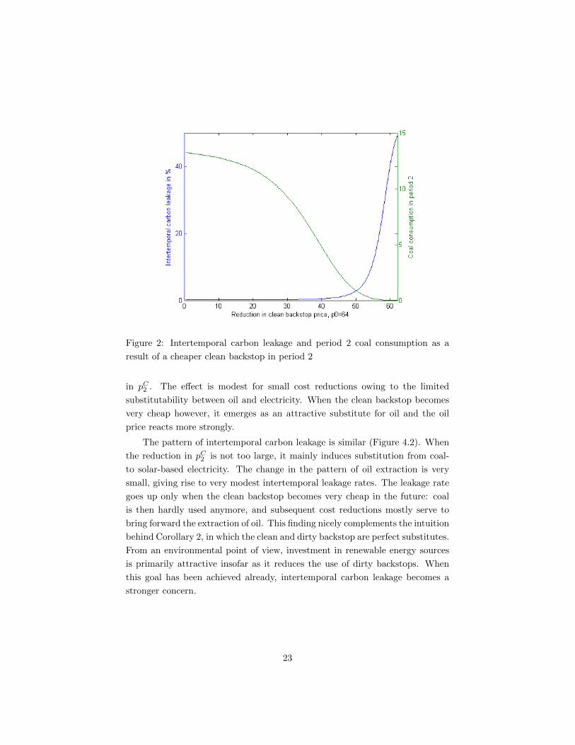
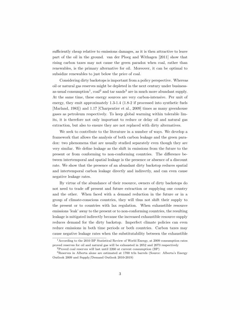
Figure 2: Intertemporal carbon leakage and period 2 coal consumption as a
result of a cheaper clean backstop in period 2
in pC2 . The effect is modest for small cost reductions owing to the limited
substitutability between oil and electricity. When the clean backstop becomes
very cheap however, it emerges as an attractive substitute for oil and the oil
price reacts more strongly.
The pattern of intertemporal carbon leakage is similar (Figure 4.2). When
the reduction in pC2 is not too large, it mainly induces substitution from coal-
to solar-based electricity. The change in the pattern of oil extraction is very
small, giving rise to very modest intertemporal leakage rates. The leakage rate
goes up only when the clean backstop becomes very cheap in the future: coal
is then hardly used anymore, and subsequent cost reductions mostly serve to
bring forward the extraction of oil. This finding nicely complements the intuition
behind Corollary 2, in which the clean and dirty backstop are perfect substitutes.
From an environmental point of view, investment in renewable energy sources
is primarily attractive insofar as it reduces the use of dirty backstops. When
this goal has been achieved already, intertemporal carbon leakage becomes a
stronger concern.
23
5 Conclusion
In this paper we employed a stylized model to analyze carbon leakage in the
presence of an abundant dirty backstop such as coal or uncoventional oil. Our
framework can be used to study both intertemporal and spatial carbon leakage.
Whereas the result from the green paradox literature that the development of a
clean backstop or an anticipated carbon tax can speed up extraction of oil and
natural gas is insightful, it might overstate the adverse consequences of these
policies by not taking into account their potential to reduce emissions from coal
and unconventional oil.
Though a carbon tax increases the price of oil and natural gas, the price
of coal goes up even more. The effect of an anticipated carbon tax on oil and
gas demand, and thus on the intertemporal extraction pattern, depends on the
relative strength of a direct own-price and an indirect substitution (from coal
to oil and gas) effect. When improved technology (e.g. diesel from coal) makes
coal a better substitute for oil in the future than it is today, intertemporal
leakage may become negative: anticipated carbon taxes cause substitution from
coal to oil in the future and thus induce oil owners to delay extraction, but the
reduction in present oil supplies does not trigger a large increase in present coal
demand as coal is still a poor substitute for oil today.
Our calibrations suggest that if a future carbon increases present emissions,
the effect is relatively small. When climate policies are spatially imperfect (only
some countries impose a carbon tax), we find much lower carbon leakage rates
than the 100% that would obtain in a model with only one exhaustible resource
that is supplied perfectly inelastically, as non-adopting countries compensate
increased emissions from one energy type with lower emissions from another.
The future availability of a clean backstop lowers dirty backstop emissions
directly (through substitution from the dirty to the clean backstop) and in-
directly (the clean backstop reduces oil prices, which encourages substitution
away from dirty backstops). These effects can become even more important
when dirty backstops are an even more prominent source of energy in the future.
Anticipated cost reductions for clean backstops are likely to increase emissions
initially, but the reduction in future emissions is considerably larger (as in the
case of future caron taxes). Our results suggest that climate policies are worth-
while even if it is not possible to instate all-encompassing carbon constraints.
24
References
M. H. Babiker. Climate change policy, market structure, and carbon leakage.
Journal of International Economics, 65(2):421–455, 2005.
S. Barrett. Self-enforcing international environmental agreements. Oxford
Economic Papers, 46:878–894, 1994.
K. Blok. Renewable energy policies in the european union. Energy Policy, 34:
251–255, 2006.
J. Burniaux and J. Oliveira Martins. Carbon emission leakages: a general equi-
librium view. OECD Economics Department Working Paper 242, 2000.
A. D. Charpentier, J. A. Bergerson, and H. A. MacLean. Understanding
the canadian oil sands industry’s greenhouse gas emissions. Environmental
Research Letters, 4:014005, 2009.
C. Di Maria, S. Smulders, and E. van der Werf. Absolute abundance and relative
scarcity: Announced policy, resource extraction, and carbon emissions. Nota
di Lavoro 92, 2008.
T. Eichner and R. Pethig. Carbon leakage, the green paradox and perfect future
markets. CESifo Working Paper 2542, 2009.
S. Felder and T. F. Rutherford. Unilateral co2 reductions and carbon leakage:
The consequences of international trade in oil and basic materials. Journal of
Environmental Economics and Management, 25:162–176, 1993.
C. Fischer and A. K. Fox. Comparing policies to combat emissions leakage:
Border tax adjustments versus rebates, 2009. Resources for the Future.
C. Fischer and S. Salant. On hotelling, emissions leakage, and climate policy
alternatives. 2010.
R. Gerlagh. Too much oil? CESifo Economic Studies, 57(1):79–102, 2011.
R. Gerlagh and O. Kuik. Carbon leakage with international technology
spillovers. Nota di Lavoaro 33.2007.
R. Golombek and M. Hoel. Unilateral emission reductions and cross-country
technology spillovers. Advances in Economic Analysis & Policy 4(2), article
3, 2004.
25
R. Q. Grafton, T. Kompas, and N. V. Long. Biofuels subsidies and the green
paradox. CESifo Working Paper 2960, 2010.
V. Hall. Major oecd country industrial sector interfuel substitution estimates,
1960-79. Energy Economics, 8(2):74–89, 1986.
J. Hill, E. Nelson, D. Tilman, S. Polasky, and D. Tiffany. Environmental,
economic, and energetic costs and benefits of biodiesel and ethanol biofuels.
Proceedings of the National Academy of Sciences of the United States of
America, 103(30):11206–11210, 2006.
M. Hoel. Efficient climate policy in the presence of free riders. Journal of
Environmental Economics and Management, 27(3):259–274, 1994.
M. Hoel. Bush meets hotelling: Effects of improved renewable energy technology
on greenhouse gas emissions. CESifo Working Paper 2492, 2008.
M. Hoel. Is there a green paradox? CESifo Working Paper 3168, 2010.
M. Hoel and S. Kverndokk. Depletion of fossil fuels and the impacts of global
warming. Resource and Energy Economics, 18:115–136, 1996.
IEA. World energy outlook, 2010.
W. J. Keller. A nested CES-type utility function and its demand and price-index
functions. European Economic Review, 7:175–186, 1976.
C. Kemfert and H. Welsch. Energy-capital-labor substitution and the economic
effects of co2 abatement: Evidence from germany. Journal of Policy Modeling,
22(6):641–660, 2000.
O. Kuik and M. Hofkes. Border adjustment for european emissions trading:
Competitiveness and carbon leakage. Energy Policy, 38:1741–1748, 2010.
J. R. Magnus and A. D. Woodland. Inter-fuel substitution in dutch manufac-
turing. Applied Economics, 19:1639–1664, 1987.
G. Marland. Carbon dioxide emission rates for conventional and synthetic fuels.
Energy, 8(12):981–992, 1983.
S. V. Paltsev. The kyoto protocol: regional and sectoral contributions to the
carbon leakage. The Energy Journal, 22:53–79, 2001.
26
T. A. Persson, C. Azar, D. Johansson, and K. Lindgren. Major oil exporters
may profit rather than lose, in a carbon-constrained world. Energy Policy,
35:6346–6353, 2007.
R. S. Pindyck. Interfuel substitution and the industrial demand for energy: An
international comparison. Review of Economics and Statistics, 61(2):169–179,
1979.
P. Renou-Maissant. Interfuel competition in the industrial sector of seven oecd
countries. Energy Policy, 27(2):99–110, 1999.
H.-W. Sinn. Das grune Paradoxon, Pladoyer fur eine illusionsfreie Klimapolitik.
Econ-Verlag, 2008a.
H.-W. Sinn. Public policies against global warming: a supply side approach.
International Tax and Public Finance, 15(4):360–394, 2008b.
J. Strand. Technology treaties and fossil-fuels extraction. The Energy Journal,
28:129–142, 2007.
N. D. Uri. Energy demand and interfuel substitution in the united kingdom.
Socio-Economic Planning Sciences, 16(4):157–162, 1982.
F. van der Ploeg and C. Withagen. Is there really a green paradox? CESifo
Working Paper 2963, 2009.
F. van der Ploeg and C. Withagen. Optimal carbon tax with a dirty backstop:
Oil, coal or renewables? CESifo Working Paper 3334, 2011.
A Appendix
A.1 Cross-Effects
In this section, we show that cross-effects are symmetric if we can define a
demand function for a composite good Y that is produced from the three energy
types according to a homogeneous function. Let
~q =
qF
qZ
qC
, ~p =
pF
pZ
pC
27
The production function for the composite good is Y = f (~q). Define the con-
ditional expenditure function e (Y, ~p) as the minimum cost to produce Y given
prices ~p. Then conditional demand for energy types exhibits symmetric cross-
effects:∂e
∂pi= qi ≡ Di (Y, ~p)
∂e2
∂pi∂pj=∂Di
∂pj=∂Dj
∂pi
By homogeneity of f (~q), we have
∂Di
∂Y= Di (1, ~p)
Let π (~p) be the price of Y . Since f (~q) is homogeneous
∂π
∂pi= Di (1, ~p)
Lastly, define demand for the composite good DY (π (~p)) and the unconditional
demand for energy types Di (~p) = Di(DY (π (~p)) , ~p
). Then
∂Di
∂pj=∂Di
∂Y
∂DY
∂π
∂π
∂pj+∂Di
∂pj= Di (1, ~p)
∂Y
∂πDj (1, ~p) +
∂Di
∂pj
∂Dj
∂pi=∂Dj
∂Y
∂DY
∂π
∂π
∂pi+∂Dj
∂pi= Dj (1, ~p)
∂Y
∂πDi (1, ~p) +
∂Dj
∂pi
Since the conditional cross-effects are equal, the unconditional cross-effects are
also equal.
A.2 Proposition 1
Proof. Period 1 emissions only depend on pC2 through qF1 , so the weak green
paradox does not occur when∂qF1∂w2
= 0. A necessary and sufficient condition for∂qF1∂w2
< 0 is that the tax increases demand for the exhaustible resource at current
prices:∂DF
2
∂w2> 0
⇔ ζF∂DF
2
∂pF+ ζZ
∂DF2
∂pZ> 0
Here we can see that period 2 extraction increases if the indirect (substitu-
tion from the dirty backstop to the exhaustible resource) outweighs the direct
28
(a higher effective exhaustible resource price) effect of the tax on exhaustible
resource demand. Rearranging and using (A.4) gives
ζF
ζZ< −
∂DZ2
∂pF
∂DF2
∂pF
The condition for the weak green paradox is
∂E1
∂w2= ζF
∂qF1∂w2
+ ζZ∂DZ
1
∂pF∂ψ1
∂qF1
∂qF1∂w2
< 0 (16)
Taking into account the sign of∂qF1∂w2
and using (3), this translates intoζFζZ
+
∂DZ1
∂pF
∂DF1
∂pF
ζFζZ
+
∂DZ2
∂pF
∂DF2
∂pF
> 0
A.3 Proposition 2
Proof. The tax w2 cannot increase the price of the exhaustible resource more
than that of the dirty backstop
∂pF2∂w2
<∂pZ
∂w2(17)
If the inequality were reversed, exhaustible resource demand would go down in
period 2 by (A.3). The period 2 gross price of the exhaustible resource goes up,
so for owners to remain indifferent between extracting in either period (8), so
must the period 1 price. Demand would go down in both periods, which would
violate the full extraction requirement. The same argument can be used to show
that (17) and (A.3) entail∂DZ
2
∂w2< 0, which proves (i). It is then straightforward
that (ii) and (iii) hold if period 2 exhaustible resource extraction decreases
(∂qF1∂w2
> 0). We proceed to prove (ii) and (iii) if∂qF1∂w2
< 0. The effect of w2 on
E2 is∂E2
∂w2=∂DZ
2
∂w2ζZ +
∂[S − qF1
]∂w2
ζF
=(ζZ)2 ∂DZ
2
∂pZ+ ζZ
∂DZ2
∂pF
(∂ψ2
∂qF1
∂qF1∂w2
+∂ψ2
∂w2
)− ζF ∂q
F1
∂w2
By the chain rule ∂ψ2
∂w2can be rewritten as ζZ ∂ψ2
∂pZ, to which we can apply (4)
=(ζZ)2 ∂DZ
2
∂pZ+ ζZ
∂DZ2
∂pF
(∂ψ2
∂qF1
∂qF1∂w2
− ζZ∂DF
∂pZ
∂DF
∂pF
)− ζF ∂q
F1
∂w2(18)
29
In this expression, the first two terms are negative and the last two terms are
positive. The first term outweighs the third term by (A.3) and the second term
outweighs the fourth term (this follows from Proposition 1 and our assumption
that∂qF1∂w2
< 0). This completes the proof of (ii). Notice that since the tax reduces
period 2 emissions, the strong green paradox implies the weak green paradox (as
in section 4). To prove (iii), we must show that ∂∂w2
[DZ
1 +DZ2
]< 0 (total use
of the dirty backstop goes down) when∂qF1∂w2
< 0 (which implies that exhaustible
resource prices rise in both periods), i.e. that
∂DZ1
∂pF∂ψ1
∂qF1
∂qF1∂w2
+ (1 + r)∂DZ
2
∂pF∂ψ1
∂qF1
∂qF1∂w2
+ ζZ∂DZ
2
∂pZ< 0 (19)
In order to back out the change exhaustible resource extraction∂qF1∂w2
, substitute
the equilibrium exhaustible resource price in (8) and totally differentiate with
respect to w2
∂ψ1
∂qF1
∂qF1∂w2
=1
1 + r
(∂ψ2
∂w2+∂ψ2
∂qF1
∂qF1∂w2
− ζF)
∂ψ1
∂qF1
∂qF1∂w2
=1
1 + r
(ζZ∂ψ2
∂pZ+∂ψ2
∂qF1
∂qF1∂w2
− ζF)
(20)
We then find∂qF1∂w2
=ζF − ζZ ∂ψ2
∂pZ
∂ψ2
∂qF1− (1 + r) ∂ψ1
∂qF1
(21)
Here, apply (3) and (4) and multiply the numerator and denominator with∂DF
2
∂pF
∂qF1∂w2
=
ζF∂DF
2
∂pF+ ζZ
∂DF2
∂pZ
−1− (1 + r)
∂DF2
∂pF
∂DF1
∂pF
Substitute in (19)
−∂DZ
1
∂pF+ (1 + r)
∂DZ2
∂pF
∂DF1
∂pF+ (1 + r)
∂DF2
∂pF
(ζF∂DF
2
∂pF+ ζZ
∂DF2
∂pZ
)+ ζZ
∂DZ2
∂pZ< 0
The fraction is smaller than one (A.3). The term in brackets is positive (since
we assumed∂qF1∂w2
< 0). Then the inequality is satisfied (−ζZ ∂DZ2
∂pZ> ζZ
∂DF2
∂pZ>
ζF∂DF
2
∂pF+ ζZ
∂DF2
∂pZ). The condition for the strong green paradox is analogous to
30
Proposition 5 with one caveat: if∂qF1∂w2
< 0, the sign of the inequality changes.ζFζZ
+
∂DZ1
∂pF∂ψ1
∂qF1
∂qF1∂w2
+ β(
(1 + r)∂DZ
2
∂pF∂ψ1
∂qF1
∂qF1∂w2
+ ζZ∂DZ
2
∂pZ
)(1− β)
∂qF1∂w2
(−ζF ∂DF2
∂pFζZ∂DF
2
∂pZ
)> 0
Divide both the numerator and denominator of the second part of the first term
by∂qF1∂w2
and substitute (21)ζF
ζZ+
∂DZ1
∂pF+ β
(1 + r)∂DZ
2
∂pF+ ζZ
∂DZ2
∂pZ
−∂DF1
∂pF− (1 + r)
∂DF2
∂pF
ζF∂DF
2
∂pF− ζZ ∂D
F2
∂pz
(1− β)
∂DF1
∂pF
ζFζZ
+
∂DZ2
∂pF
∂DF2
∂pF
> 0
A.4 Proposition 3
Proof. Analogous to Propositions 1 and 2
A.5 Proposition 4
Proof. Determine the condition for ∂E1
∂pC2< 0
∂E1
∂pC2= ζF
∂qF1∂pC2
+ ζZ∂DZ
1
∂pF∂ψ1
∂qF1
∂qF1∂pC2
< 0 (22)
⇔ ∂qF1∂pC2
(ζF + ζZ
∂DZ1
∂pF∂ψ1
∂qF1
)< 0
∂qF1∂pC2
is negative by (A.3), so the term in brackets must be positive for the weak
green paradox to materialize: A reduction in pC2 increases period 1 exhaustible
resource extraction
ζF > −ζZ ∂DZ1
∂pF∂ψ1
∂qF1
ζF
ζZ> −
∂DZ
∂pF
∂DF
∂pF
31
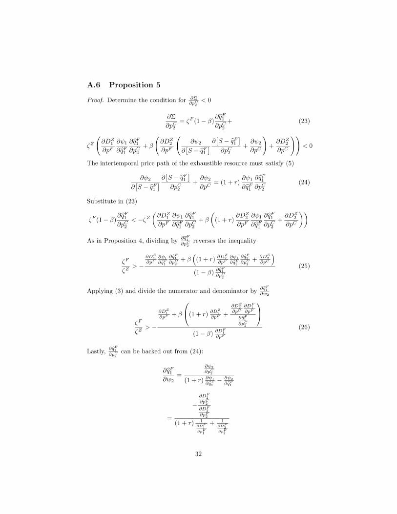
A.6 Proposition 5
Proof. Determine the condition for ∂Σ∂pC2
< 0
∂Σ
∂pC2= ζF (1− β)
∂qF1∂pC2
+ (23)
ζZ
(∂DZ
1
∂pF∂ψ1
∂qF1
∂qF1∂pC2
+ β
(∂DZ
2
∂pF
(∂ψ2
∂[S − qF1
] ∂[S − qF1 ]∂pC2
+∂ψ2
∂pC
)+∂DZ
2
∂pC
))< 0
The intertemporal price path of the exhaustible resource must satisfy (5)
∂ψ2
∂[S − qF1
] ∂[S − qF1 ]∂pC2
+∂ψ2
∂pC= (1 + r)
∂ψ1
∂qF1
∂qF1∂pC2
(24)
Substitute in (23)
ζF (1− β)∂qF1∂pC2
< −ζZ(∂DZ
1
∂pF∂ψ1
∂qF1
∂qF1∂pC2
+ β
((1 + r)
∂DZ2
∂pF∂ψ1
∂qF1
∂qF1∂pC2
+∂DZ
2
∂pC
))As in Proposition 4, dividing by
∂qF1∂pC2
reverses the inequality
ζF
ζZ> −
∂DZ1
∂pF∂ψ1
∂qF1
∂qF1∂pC2
+ β(
(1 + r)∂DZ
2
∂pF∂ψ1
∂qF1
∂qF1∂pC2
+∂DZ
2
∂pC
)(1− β)
∂qF1∂pC2
(25)
Applying (3) and divide the numerator and denominator by∂qF1∂w2
ζF
ζZ> −
∂DZ1
∂pF+ β
(1 + r)∂DZ
2
∂pF+
∂DZ2
∂pC∂DF
1
∂pF
∂qF1∂pC2
(1− β)
∂DF1
∂pF
(26)
Lastly,∂qF1∂pC2
can be backed out from (24):
∂qF1∂w2
=
∂ψ2
∂pC2
(1 + r) ∂ψ1
∂qF1− ∂ψ2
∂qF1
=
−∂DF
2
∂pC2∂DF
2
∂pF2
(1 + r) 1∂DF
1∂pF1
+ 1∂DF
2∂pF2
32
= −∂DF
2
∂pC2
(1 + r)
∂DF2
∂pF
∂DF1
∂pF
+ 1
Substitute in (26), so that the final condition becomes
ζF
ζZ> −
∂DZ1
∂pF+ β
((1 + r)
∂DZ2
∂pF+
∂DZ2
∂pC
∂DF2
∂pC
[−(
1 + r)∂DF
2
∂pF−∂D
F1
∂pF
])(1− β)
∂DF1
∂pF
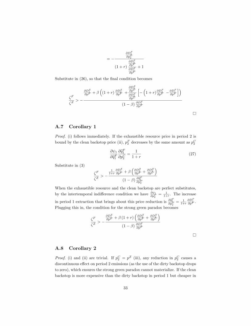
A.7 Corollary 1
Proof. (i) follows immediately. If the exhaustible resource price in period 2 is
bound by the clean backstop price (ii), pF2 decreases by the same amount as pC2
∂ψ1
∂qF1
∂qF1∂pC2
=1
1 + r(27)
Substitute in (3)
ζF
ζZ> −
11+r
∂DZ1
∂pF+ β
(∂DZ
2
∂pF+
∂DZ2
∂pC
)(1− β)
∂qF1∂pC2
When the exhaustible resource and the clean backstop are perfect substitutes,
by the intertemporal indifference condition we have ∂ψ1
∂pC2= 1
1+r . The increase
in period 1 extraction that brings about this price reduction is∂qF1∂pC2
= 11+r
∂DF1
∂pF.
Plugging this in, the condition for the strong green paradox becomes
ζF
ζZ> −
∂DZ1
∂pF+ β (1 + r)
(∂DZ
2
∂pF+
∂DZ2
∂pC
)(1− β)
∂DF1
∂pF
A.8 Corollary 2
Proof. (i) and (ii) are trivial. If pC2 = pZ (iii), any reduction in pC2 causes a
discontinuous effect on period 2 emissions (as the use of the dirty backstop drops
to zero), which ensures the strong green paradox cannot materialize. If the clean
backstop is more expensive than the dirty backstop in period 1 but cheaper in
33
period 2 (iv), the dirty backstop is not used in the second period, which means
the β(
(1 + r)∂DZ
2
∂pF2
∂ψ1
∂qF1
∂qF1∂pC2
+∂DZ
2
∂pC
)term in (13) is equal to zero. The
∂qF1∂pC2
terms
in the numerator and denominator then cancel out, so the condition for the
strong green paradox becomes
ζF
ζZ> −
∂DZ1
∂pF∂ψ1
∂qF1
1− β(28)
A.9 Corollary 3
Proof. If the exhaustible resource price would always be lower than pZ (i), the
model is equivalent to a setting without the dirty backstop, and we have both
green paradoxes for the usual reasons. Under (ii), the dirty backstop is only
used in the second period (if the exhaustible resource and dirty backstop prices
are equal in period 2, the exhaustible resource must be cheaper in period 1 by
(5)). Because exhaustible resource owners are first-movers and residual demand
is fulfilled by the dirty backstop, a reduction in period 2 green backstop costs
only reduces demand for the dirty backstop. The optimal extraction path is not
affected, and since we assumed ζZ > ζF neither the weak nor the strong green
paradox occurs.
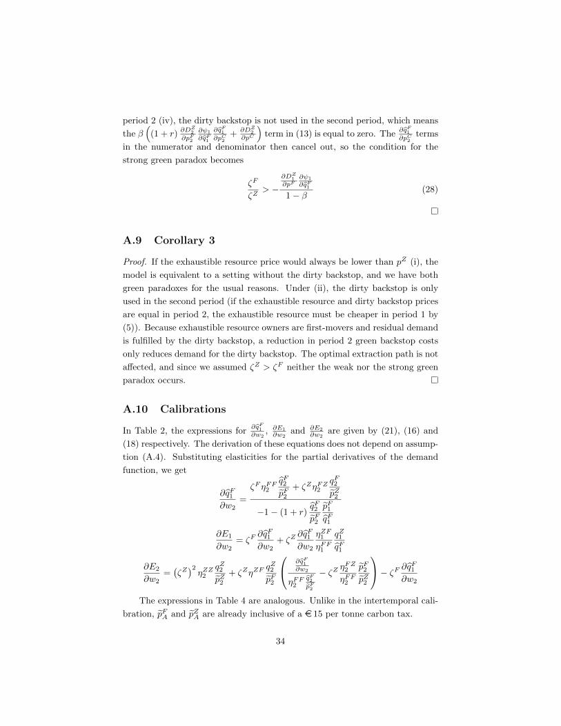
A.10 Calibrations
In Table 2, the expressions for∂qF1∂w2
, ∂E1
∂w2and ∂E2
∂w2are given by (21), (16) and
(18) respectively. The derivation of these equations does not depend on assump-
tion (A.4). Substituting elasticities for the partial derivatives of the demand
function, we get
∂qF1∂w2
=
ζF ηFF2
qF2pF2
+ ζZηFZ2
qF2pZ2
−1− (1 + r)qF2pF2
pF1qF1
∂E1
∂w2= ζF
∂qF1∂w2
+ ζZ∂qF1∂w2
ηZF1
ηFF1
qZ1qF1
∂E2
∂w2=(ζZ)2ηZZ2
qZ2pZ2
+ ζZηZFqZ2pF2
∂qF1∂w2
ηFF2qF2pF2
− ζZ ηFZ2
ηFF2
pF2pZ2
− ζF ∂qF1∂w2
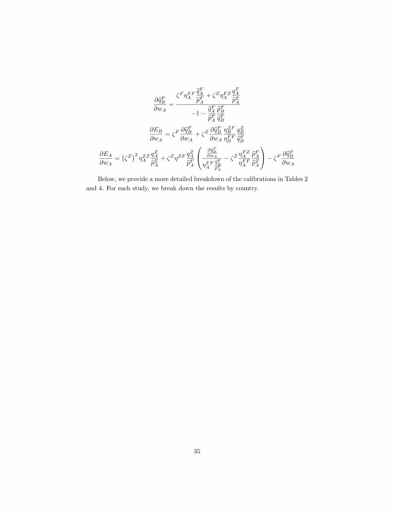
The expressions in Table 4 are analogous. Unlike in the intertemporal cali-
bration, pFA and pZA are already inclusive of a e 15 per tonne carbon tax.
34
∂qFB∂wA
=
ζF ηFFAqFApFA
+ ζZηFZAqFApZA
−1− qFApFA
pFBqFB
∂EB∂wA
= ζF∂qFB∂wA
+ ζZ∂qFB∂wA
ηZFBηFFB
qZBqFB
∂EA∂wA
=(ζZ)2ηZZA
qZApZA
+ ζZηZFqZApFA
∂qFB∂wA
ηFFAqFApFA
− ζZ ηFZA
ηFFA
pFApZA
− ζF ∂qFB∂wA
Below, we provide a more detailed breakdown of the calibrations in Tables 2
and 4. For each study, we break down the results by country.
35
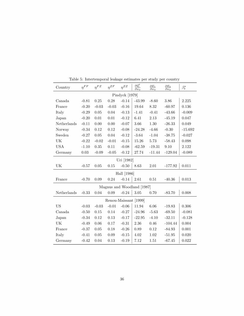
Table 5: Intertemporal leakage estimates per study per country
Country ηFF ηFZ ηZF ηZZ∂qF1∂w2
∂E1
∂w2
∂E2
∂w2β∗t
Pindyck [1979]
Canada -0.81 0.25 0.28 -0.14 -43.99 -8.60 3.86 2.225
France -0.20 -0.03 -0.03 -0.16 19.64 8.32 -60.97 0.136
Italy -0.29 0.05 0.04 -0.13 -1.41 -0.41 -43.66 -0.009
Japan -0.20 0.01 0.01 -0.12 6.41 2.13 -45.19 0.047
Netherlands -0.11 0.00 0.00 -0.07 3.66 1.30 -26.33 0.049
Norway -0.34 0.12 0.12 -0.08 -24.28 -4.66 -0.30 -15.692
Sweden -0.27 0.05 0.04 -0.12 -3.64 -1.04 -38.75 -0.027
UK -0.22 -0.02 -0.01 -0.15 15.26 5.73 -58.43 0.098
USA -1.10 0.35 0.11 -0.08 -62.59 -19.31 9.10 2.122
Germany 0.03 -0.09 -0.05 -0.12 27.74 -11.44 -129.04 -0.089
Uri [1982]
UK -0.57 0.05 0.15 -0.50 8.63 2.01 -177.92 0.011
Hall [1986]
France -0.70 0.09 0.24 -0.14 2.61 0.51 -40.36 0.013
Magnus and Woodland [1987]
Netherlands -0.33 0.04 0.09 -0.24 3.05 0.70 -83.70 0.008
Renou-Maissant [1999]
US -0.03 -0.03 -0.01 -0.06 11.94 6.06 -19.83 0.306
Canada -0.50 0.15 0.14 -0.27 -24.96 -5.63 -69.50 -0.081
Japan -0.34 0.12 0.13 -0.17 -22.95 -4.10 -32.11 -0.128
UK -0.49 0.06 0.17 -0.31 2.36 0.46 -104.44 0.004
France -0.37 0.05 0.18 -0.26 0.89 0.12 -84.93 0.001
Italy -0.41 0.05 0.09 -0.15 4.02 1.02 -51.95 0.020
Germany -0.42 0.04 0.13 -0.19 7.12 1.51 -67.45 0.022
36
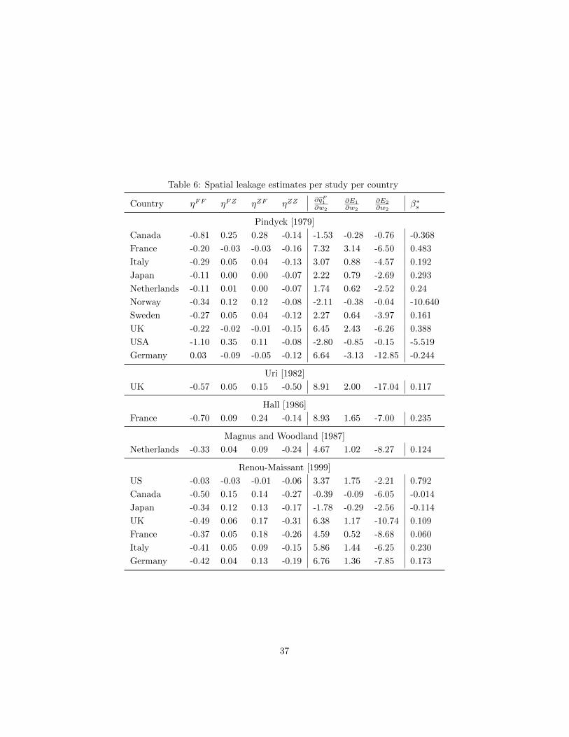
Table 6: Spatial leakage estimates per study per country
Country ηFF ηFZ ηZF ηZZ∂qF1∂w2
∂E1
∂w2
∂E2
∂w2β∗s
Pindyck [1979]
Canada -0.81 0.25 0.28 -0.14 -1.53 -0.28 -0.76 -0.368
France -0.20 -0.03 -0.03 -0.16 7.32 3.14 -6.50 0.483
Italy -0.29 0.05 0.04 -0.13 3.07 0.88 -4.57 0.192
Japan -0.11 0.00 0.00 -0.07 2.22 0.79 -2.69 0.293
Netherlands -0.11 0.01 0.00 -0.07 1.74 0.62 -2.52 0.24
Norway -0.34 0.12 0.12 -0.08 -2.11 -0.38 -0.04 -10.640
Sweden -0.27 0.05 0.04 -0.12 2.27 0.64 -3.97 0.161
UK -0.22 -0.02 -0.01 -0.15 6.45 2.43 -6.26 0.388
USA -1.10 0.35 0.11 -0.08 -2.80 -0.85 -0.15 -5.519
Germany 0.03 -0.09 -0.05 -0.12 6.64 -3.13 -12.85 -0.244
Uri [1982]
UK -0.57 0.05 0.15 -0.50 8.91 2.00 -17.04 0.117
Hall [1986]
France -0.70 0.09 0.24 -0.14 8.93 1.65 -7.00 0.235
Magnus and Woodland [1987]
Netherlands -0.33 0.04 0.09 -0.24 4.67 1.02 -8.27 0.124
Renou-Maissant [1999]
US -0.03 -0.03 -0.01 -0.06 3.37 1.75 -2.21 0.792
Canada -0.50 0.15 0.14 -0.27 -0.39 -0.09 -6.05 -0.014
Japan -0.34 0.12 0.13 -0.17 -1.78 -0.29 -2.56 -0.114
UK -0.49 0.06 0.17 -0.31 6.38 1.17 -10.74 0.109
France -0.37 0.05 0.18 -0.26 4.59 0.52 -8.68 0.060
Italy -0.41 0.05 0.09 -0.15 5.86 1.44 -6.25 0.230
Germany -0.42 0.04 0.13 -0.19 6.76 1.36 -7.85 0.173
37