c© 2012

Nadide Banu Olcay

ALL RIGHTS RESERVED

ESSAYS ON PRINCIPAL-AGENT MODELS

BY NADIDE BANU OLCAY

A dissertation submitted to the

Graduate School—New Brunswick

Rutgers, The State University of New Jersey

in partial fulfillment of the requirements

for the degree of

Doctor of Philosophy

Graduate Program in Economics

Written under the direction of

Professor Tomas Sjostrom

and approved by

New Brunswick, New Jersey

May, 2012

ABSTRACT OF THE DISSERTATION

Essays on Principal-Agent Models

by Nadide Banu Olcay

Dissertation Director: Professor Tomas Sjostrom

This dissertation consists of three chapters on principal-agent models. Chapter 2 studies

a dynamic optimal contract design problem whereas chapter 3 is an empirical investiga-

tion of the incentive contracts in the market of top executives. Chapter 4 is a theoretical

chapter exploring welfare impacts of the structure in the top-level bureaucracy.

In chapter 1, I consider a dynamic moral hazard model where the principal offers a

series of short-run contracts. I study the optimal mix of two alternative instruments for

incentive provision: a performance based wage (a “carrot”) and a termination threat

(a “stick”). Both carrot and stick, which act as substitutes for each other, are used

more intensively as the agent approaches the end of her finite life. The sharing of the

surplus from the relationship plays a key role: a termination threat is included in the

optimal contract if and only if the agent’s expected future gain from the relationship is

sufficiently high, compared to the principal’s expected future gain. Also, a termination

threat is more likely to be optimal if output depends more on “luck” than on effort, if

the discount factor is high, or if the agent’s productivity is low.

Chapter 3 is an empirical study with a focus on the use of direct pay and forced

turnover in executive contracting and how they depend on tenure and managerial ability.

Managerial ability is proxied by the age at the time of promotion and by “reputation”

which rely on media citations. I find that pay increases with tenure, yet there is no

ii

strong evidence that termination threat follows a particular time pattern. A better

reputation increases pay and decreases the likelihood of forced turnover. Managerial

ability, as both proxied by age-at-promotion for insiders and by reputation for outsiders,

decreases the likelihood of forced turnover.

Chapter 4 investigates the welfare implications of multiple principals in the highest

level of bureaucracy. The existence of multiple principals generates a “common agency”.

The analysis reveals that the optimal hierarchy depends on the existence of “rents” from

office that the principals enjoy: a single-principal model dominates common agency only

if there are positive rents.

iii

Acknowledgements

It is hardly possible to adequately thank my advisor, Prof. Tomas Sjostrom, without

whom this work would have simply been impossible. But as far as the words allow

me to express my gratitude, I am profoundly thankful for providing compassionate

supervision, guidance and inspiration on every stage of this thesis, which was leaving me

in admiration of his inexhaustible energy and persistent enthusiasm; for persuading me

to believe that my ideas are valuable and the confidence he placed in me; for his endless

patience in helping me to write papers; and for his unflagged interest in my research

even at the times of slow progress. Throughout my entire graduate life at Rutgers, it

has been both a great experience to have such a positively challenging instructor and a

blessing to have the chance to benefit from his sharp intellect, knowledge, intelligence

and wisdom.

I am also grateful to Prof. Carolyn Moehling for her encouragement and guidance

on my empirical chapter. Without her advice and her patience regarding my lack of

experience on empirical work, this chapter would not be as it is. I am also thankful to

Prof. Colin Campbell for providing valuable suggestions and discussions which helped to

improve my papers. Prof. Kalyan Chatterjee, as the outsider reader of my dissertation

committee, and Prof. Mark Killingsworth, are also gratefully acknowledged for their

helpful comments.

My deepest gratitude to Prof. Ismail Saglam for inspiring me towards studying

economics at the graduate level. His research enthusiasm and his constant support to

his students will always be an example for me to follow. I am also thankful to Prof.

Fikret Adaman for his mentorship on my pursuits towards a graduate study.

I would like to specially thank Dorothy Rinaldi for her encouragement and support

in my graduate life. She was more than an administrative staff for all of the graduate

iv

students.

I would never reach to this point in my life without endless love and unconditional

support of my parents. I also would like to thank my brother for especially facilitating

my trips back home, and to Bengi for her constant moral support. A special thanks

goes to my dear Esra who were always there for me even we are miles apart. Many

thanks to my long-time friend, Oylum for sharing both the pain and the joy; to Basak

for her patience and help at the rough times, and to Nil and Dilara, without whom

my last year at Rutgers would be unthinkable. Meric, Bahar, Gokce, and many other

friends at Rutgers, made me feel lucky to have been surrounded by them; thanks to all.

v

Dedication

To my mother, Ayse Selda Olcay ; and my father, Gurol Olcay.

vi

Table of Contents

Abstract . . . . . . . . . . . . . . . . . . . . . . . . . . . . . . . . . . . . . . . . ii

Acknowledgements . . . . . . . . . . . . . . . . . . . . . . . . . . . . . . . . . iv

Dedication . . . . . . . . . . . . . . . . . . . . . . . . . . . . . . . . . . . . . . . vi

List of Tables . . . . . . . . . . . . . . . . . . . . . . . . . . . . . . . . . . . . . x

List of Figures . . . . . . . . . . . . . . . . . . . . . . . . . . . . . . . . . . . . xi

1. Introduction . . . . . . . . . . . . . . . . . . . . . . . . . . . . . . . . . . . 1

2. Dynamic Incentive Contracts with Termination Threats . . . . . . . 9

2.1. Introduction . . . . . . . . . . . . . . . . . . . . . . . . . . . . . . . . . 9

2.2. The Model . . . . . . . . . . . . . . . . . . . . . . . . . . . . . . . . . . 16

2.2.1. Dynamics of the Equilibrium . . . . . . . . . . . . . . . . . . . . 24

2.2.2. The Equilibrium Path: Main Theorem . . . . . . . . . . . . . . . 28

2.3. Proof of Theorem 5 . . . . . . . . . . . . . . . . . . . . . . . . . . . . . . 32

2.3.1. Equilibrium path with q(t) = 0 for all t . . . . . . . . . . . . . . 33

2.3.2. Equilibrium path with q(t) = 1 for all t . . . . . . . . . . . . . . 35

2.3.3. “Mixed” equilibrium path . . . . . . . . . . . . . . . . . . . . . . 40

Optimal Firing Rule for the “Mixed” Equilibrium . . . . . . . . 42

2.3.4. Summary of the analysis . . . . . . . . . . . . . . . . . . . . . . . 46

2.4. Comparative Dynamics . . . . . . . . . . . . . . . . . . . . . . . . . . . 50

2.4.1. A change in quality differential . . . . . . . . . . . . . . . . . . . 50

2.4.2. A change in luck . . . . . . . . . . . . . . . . . . . . . . . . . . . 55

2.4.3. A change in discount rate . . . . . . . . . . . . . . . . . . . . . . 60

a. High productivity . . . . . . . . . . . . . . . . . . . . . . . . . 60

vii

b. Moderate productivity . . . . . . . . . . . . . . . . . . . . . . 60

c. Low productivity . . . . . . . . . . . . . . . . . . . . . . . . . 64

d. Summary of the effect of a change in r . . . . . . . . . . . . . 65

2.5. Concluding Comments . . . . . . . . . . . . . . . . . . . . . . . . . . . . 67

3. Incentivizing CEOs via Pay and Forced Turnover: Do Tenure and

Managerial Ability Matter? . . . . . . . . . . . . . . . . . . . . . . . . . . . . 68

3.1. Introduction . . . . . . . . . . . . . . . . . . . . . . . . . . . . . . . . . . 68

3.2. Data Description . . . . . . . . . . . . . . . . . . . . . . . . . . . . . . . 75

3.2.1. Sample Selection . . . . . . . . . . . . . . . . . . . . . . . . . . . 75

3.2.2. Measures for Firm Performance and Firm Level Controls . . . . 77

3.2.3. CEO Pay, Tenure and CEO Characteristics . . . . . . . . . . . . 77

3.2.4. Measures for CEO’s power on Corporate Governance . . . . . . . 78

3.2.5. Measures for CEO Ability . . . . . . . . . . . . . . . . . . . . . . 78

3.3. Analysis I: Relations of CEO Pay with Tenure and Managerial Ability . 81

3.3.1. CEO Pay and Tenure . . . . . . . . . . . . . . . . . . . . . . . . 81

a. Empirical Strategy . . . . . . . . . . . . . . . . . . . . . . . . 81

b. Results . . . . . . . . . . . . . . . . . . . . . . . . . . . . . . . 83

3.3.2. The Impact of Ability on CEO Pay and Tenure-Pay Relationship 85

a. Empirical Strategy . . . . . . . . . . . . . . . . . . . . . . . . 86

b. Results . . . . . . . . . . . . . . . . . . . . . . . . . . . . . . . 87

3.4. Analysis II: Relations of CEO Forced Turnover with Tenure and Man-

agerial Ability . . . . . . . . . . . . . . . . . . . . . . . . . . . . . . . . . 89

3.4.1. CEO Forced Turnover and Tenure . . . . . . . . . . . . . . . . . 89

a. Empirical Strategy . . . . . . . . . . . . . . . . . . . . . . . . 89

b. Results . . . . . . . . . . . . . . . . . . . . . . . . . . . . . . . 90

3.4.2. The Impact of Ability on Forced Turnover and Tenure-Forced

Turnover Relationship . . . . . . . . . . . . . . . . . . . . . . . . 93

Empirical Strategy and Results . . . . . . . . . . . . . . . . . . . 94

viii

3.5. Concluding Comments . . . . . . . . . . . . . . . . . . . . . . . . . . . . 95

Appendix A: Figures and Tables . . . . . . . . . . . . . . . . . . . . . . . . 97

Appendix B . . . . . . . . . . . . . . . . . . . . . . . . . . . . . . . . . . . . . . 121

4. Common Agency within Bureaucracy . . . . . . . . . . . . . . . . . . . 122

4.1. Introduction . . . . . . . . . . . . . . . . . . . . . . . . . . . . . . . . . . 122

4.2. The Model . . . . . . . . . . . . . . . . . . . . . . . . . . . . . . . . . . 126

4.2.1. Agent’s Problem . . . . . . . . . . . . . . . . . . . . . . . . . . . 128

4.2.2. Equilibrium in Single-Principal Model . . . . . . . . . . . . . . . 131

a. Principal’s Problem . . . . . . . . . . . . . . . . . . . . . . . . 131

b. Citizen’s Problem . . . . . . . . . . . . . . . . . . . . . . . . . 133

4.2.3. Equilibrium in Common Agency . . . . . . . . . . . . . . . . . . 151

a. Principal’s Problem . . . . . . . . . . . . . . . . . . . . . . . . 151

b. Citizen’s Problem . . . . . . . . . . . . . . . . . . . . . . . . . 154

4.3. A Comparative Assessment: One Principal or Many? . . . . . . . . . . . 158

4.4. An Extension: Full Information . . . . . . . . . . . . . . . . . . . . . . . 160

4.4.1. Equilibrium in Single-Principal Model . . . . . . . . . . . . . . . 161

4.4.2. Equilibrium in Common Agency . . . . . . . . . . . . . . . . . . 162

4.5. Concluding Remarks . . . . . . . . . . . . . . . . . . . . . . . . . . . . . 163

References . . . . . . . . . . . . . . . . . . . . . . . . . . . . . . . . . . . . . . . 166

Vita . . . . . . . . . . . . . . . . . . . . . . . . . . . . . . . . . . . . . . . . . . . 173

ix

List of Tables

3.1. Theoretical Predictions . . . . . . . . . . . . . . . . . . . . . . . . . . . . 102

3.2. CEO Turnover . . . . . . . . . . . . . . . . . . . . . . . . . . . . . . . . 103

3.3. Forced CEO Turnover . . . . . . . . . . . . . . . . . . . . . . . . . . . . 104

3.4. Descriptive Statistics . . . . . . . . . . . . . . . . . . . . . . . . . . . . . 105

3.5. CEO Performance, Pay and Tenure . . . . . . . . . . . . . . . . . . . . . 106

3.6. Proxy: Media Visibility . . . . . . . . . . . . . . . . . . . . . . . . . . . 107

3.7. Proxy: Age-at-Promotion . . . . . . . . . . . . . . . . . . . . . . . . . . 108

3.8. CEO Performance, Pay, Tenure and Reputation (Good Press (1 year)) . 109

3.9. CEO Performance, Pay, Tenure and Reputation (Good Press (3 year)) . 110

3.10. CEO Performance, Pay, Tenure and Reputation (Good Press (5 years)) 111

3.11. CEO Performance, Pay, Tenure and Reputation (Press (1 year)) . . . . 112

3.12. CEO Performance, Pay, Tenure and Reputation (Press (3 years)) . . . . 113

3.13. CEO Performance, Pay, Tenure and Reputation (Press (5 years)) . . . . 114

3.14. CEO Performance, Pay, Tenure and Ability (Age-at-Promotion) . . . . . 115

3.15. CEO Performance and Forced Turnover . . . . . . . . . . . . . . . . . . 116

3.16. CEO Performance and Forced Turnover - More Controls . . . . . . . . . 117

3.17. CEO Performance, Forced Turnover and Reputation (Good Press) . . . 118

3.18. CEO Performance, Forced Turnover and Reputation (Press) . . . . . . . 119

3.19. CEO Performance, Forced Turnover and Ability (Age-at-Promotion) . . 120

x

List of Figures

2.1. Dynamics of the Equilibrium (r = 0) . . . . . . . . . . . . . . . . . . . . 25

2.2. Dynamics of the Equilibrium (r > 0) . . . . . . . . . . . . . . . . . . . . 29

2.3. Equilibrium Path with q(t) = 0 for all t . . . . . . . . . . . . . . . . . . 35

2.4. Equilibrium Path with q(t) = 1 for all t . . . . . . . . . . . . . . . . . . 41

2.5. ”Mixed” Equilibrium Path . . . . . . . . . . . . . . . . . . . . . . . . . . 42

2.6. The Optimal Contract . . . . . . . . . . . . . . . . . . . . . . . . . . . . 49

2.7. A Change in Quality Differential . . . . . . . . . . . . . . . . . . . . . . 54

2.8. A Change in Luck . . . . . . . . . . . . . . . . . . . . . . . . . . . . . . 59

2.9. A Change in Discount Rate . . . . . . . . . . . . . . . . . . . . . . . . . 66

3.1. Tenure and CEO Pay . . . . . . . . . . . . . . . . . . . . . . . . . . . . 97

3.2. % Change in Median CEO Compensation as Tenure Increases (from “less

than 5 years” to “more than 5 years”)-Top 25% vs. Bottom 25% . . . . 98

3.3. Incidence of Forced CEO Turnover . . . . . . . . . . . . . . . . . . . . . 99

3.4. [a] Tenure and Likelihood of Forced CEO Turnover [b] Tenure and Likeli-

hood of Forced CEO Turnover (Top 25% vs. Bottom 25% Performance)

[c] Tenure and Likelihood of Forced CEO Turnover (At Top 5%, Top

25%, Bottom 25% and Bottom 5% Performance) . . . . . . . . . . . . . 100

3.5. Incidence of Forced CEO Turnover–Top 25% vs. Bottom 25% . . . . . . 101

4.1. Example: Equilibrium Outcomes for a Given Contract Option . . . . . 135

4.2. Proof of Proposition 35 . . . . . . . . . . . . . . . . . . . . . . . . . . . 144

4.3. Agent’s Effort Choice in Common Agency . . . . . . . . . . . . . . . . . 152

4.4. Equilibrium in Common Agency . . . . . . . . . . . . . . . . . . . . . . 154

4.5. Proof of Proposition 41 . . . . . . . . . . . . . . . . . . . . . . . . . . . 157

4.6. Equilibrium in Common Agency: Full Information . . . . . . . . . . . . 164

xi

1

Chapter 1

Introduction

The principal-agent framework, which is the focus of analysis presented in this study,

relies on a frequently observed real life phenomena: an economic agent’s (“the princi-

pal“) delegation of a task to another one (“the agent”), who has different objectives than

the principal, becomes problematic for the principal when she does not have perfect

information about the agent.

Incentive theory, via study of optimal contracts, attempts to find solutions to the

problems which arise due to such conflicting interests in the presence of asymmetric in-

formation. It has been a long while since the economists realized the incentive problems,

and these problems had been considered as a mere failure of the market mechanism until

they were visited within the principal-agent paradigm.

This dissertation presents three chapters within this paradigm. Chapter 2 studies

the optimal contracts in a dynamic principal-agent model while Chapter 3 is an em-

pirical analysis of the employment contracts in the market of CEOs. The last chapter

investigates the welfare implications of the two bureaucratic systems each of which has

a different type of agency problem.

Chapter 2: Dynamic Incentive Contracts with Termination Threads

In this chapter I consider a dynamic principal-agent model which is applicable to

employment contracts where the principal can use two different incentive instruments,

incentive pay and threat of termination, both of which can be contingent on perfor-

mance. Previous literature has extensively studied the provision of incentives only

through one channel, i.e. incentive pay, but not much considered alternative channels.

However, firing when the performance is not satisfactory can play an important role in

providing incentives.

2

The idea that thread of termination is a powerful incentive devise is not peculiar

to firm-employee relationships. Bank-borrower relationships where banks deny future

loans to defaulters, or landlord-tenant relationships where the landlord reacts to poor

crops by evicting the share-cropper, are other examples of the use termination as an

incentive device.

I focus on the contracts which allow the use of the two incentive tools and study

how the efficient mix of these devices changes through time. As a common real life

observation, the increasing wage-profile through a worker’s tenure on the same job

inspired many researchers to understand the reasons behind. Lazear (1979), as a first

attempt to explain the issue, develops a theoretical model where the firm fully commits

to a long-term contract specifying all future wages at the start of the firm-worker

relationship. In this setting, an upward sloping wage profile, which pays less than the

worker’s productivity in the early stages but promises to pay more towards the end

of her career, is the efficient way to provide incentives for the firm since it completely

solves the moral hazard problem.

How significant is the full-commitment assumptions in explaining upward sloping

incentive schemes? In practice, committing to a long-term contract create problems on

the firm’s side. For that reason, employment contracts are mostly renewed in shorter

terms after the performance of the employee is evaluated. Therefore, as a second

attempt to explain the issue, Gibbons and Murphy (1992) studies the optimal contracts

in the presence of short-term commitment.

In an adverse selection model, where the employee’s true ability is not known,

Gibbons and Murphy (1992) show that “career concerns” is the reason for increasing

earnings profile. When the beliefs about her ability is updated each period after observ-

ing her performance, in the early stages of her career, the employee is already highly

motivated to work hard. Then the optimal explicit incentives should be weak. However,

in the later stages, career concerns is no longer important, hence the optimal incentives

should be stronger. Gibbons and Murphy’s (1992) model is helpful to explain a real

life practice in employment contracts, yet the key point is the adverse selection and the

3

market’s ability to update its beliefs about the employee.

I maintain Gibbons and Murphy’s short-term commitment assumption. However,

I drop the career concerns dimension but add the termination threat as an alternative

incentive device and try to answer the following questions: what is the role of termina-

tion threat in a pure moral hazard model with limited commitment, and how does the

optimal use of this threat interact with explicit wage incentive in a dynamic setting?

In order to study these questions, I consider a finite horizon principal-agent model:

there is a fixed point in time when the relationship ends, where this assumption can

be understood by the date of mandatory retirement that is used widely in practice.

The model predicts that, first, the use of both incentive devices; i.e. termination

probability contingent on poor performance and performance based wage increases as

the agent is more senior in her tenure. Second, the two incentive mechanisms are used as

substitutes for each other. The theory predictions are best understood when the results

are interpreted in terms of how the surplus from the relationship is shared between the

two parties. A termination threat is included in the optimal contract if and only if the

agent’s expected future surplus from the relationship is sufficiently high, compared to

the principal expected future gain.

The main result, by relying on the share of surplus, is in the spirit of self-enforcing

contract literature which studies the optimal contract design when there is an enforce-

ment issue in the absence of verifiable outcomes. As a benchmark result in this area,

MacLeod and Malcomson (1987) show that self enforcing contracts solve the enforce-

ment problem only if the agreement can generate a surplus for at least one of the two

parties.

In contrast to these models, I assume short-term performance-based contracts are

enforceable. Also, since the agent has a finite life, the series of short-run contract is

not stationary, in contrast to MacLeod and Malcomson (1987). Towards the end of the

agent’s “life”, the expected future surplus from the relationship dwindles, and the ter-

mination threat becomes less effective. I show that even with short-term contracts and

no “career concerns”, the incentive wage and termination profiles are upward sloping.

4

That is, as the agent approaches the end of her life, the probability of termination if the

quality of output is unacceptable, and the wage when the quality is acceptable, both

increase.

Furthermore, for a given observed productivity (as a measure for “ability”), the

model provides several predictions in terms of how the two incentive devices should be

used. At a given point in time, higher ability increases pay and reduces probability

of forced turnover. The key point here is that such ability change affects the share of

surplus created by the relationship. As ability increases, principal’s surplus increases

relative to the agent’s; therefore it becomes optimal to decrease probability of termina-

tion. However, to provide sufficient incentives to work hard, the decrease in termination

probability is accompanied by the increase in incentive pay.

Chapter 3: Incentivizing CEOs via Pay and Forced Turnover: Do Tenure

and Ability Matter?

This chapter is an empirical study of the employment contracts in the market for

CEOs where short-term contracts are a common practice. The study is not a direct

test of, but mainly inspired from the theoretical results of Chapter 2, with a focus on

how the explicit incentives, in the form of total CEO pay, and the implicit incentives,

i.e. the probability of forced CEO turnover, change with tenure and managerial ability.

Executive contract design, as a research field, has attracted the interest of many

researchers mainly because of the need to optimally determine the contracts for the top-

level employees, given that they constitute a significant part of the firm’s compensation

costs. For example, the empirical evidence presents that CEO compensation has risen

dramatically beyond the rising levels of an average worker’s compensation. While the

average CEO pay at the largest companies in the US was 40 times that of the average

worker a generation ago, in 2005, the pay of top American CEOs was over 400 times

average earnings1. Boards, senior management teams, and shareholders are constantly

struggling with how to design the right type of executive compensation plans.

Both the amount of the executive pay and the organizational role of executives

1The Economist, March 3rd, 2006.

5

increase the importance of executive compensation design. As a first step to approach

this problem, the relationship between the executive and shareholders, who actually

delegated their authority to the board of directors, has been identified as a principal-

agent model. The design problem is to give the right incentives to the executives, i.e.

motivating the CEO of the firm to act in the best interests of the shareholders. For

example, if shareholders (the principals) desire to maximize their wealth as measured by

the market value of the firm’s common stock, stock options might be a way to encourage

CEOs (the agents) to work in order to increase the firm’s stock market value. Then

the task of shareholders is actually to derive the optimal contracts that would induce

results to increase the firm value.

The idea that separation of ownership and control in modern corporations can be

viewed as an agency problem was fist suggested by Berle and Means (1932). Later

Jensen and Meckling (1976) formalized this perspective. However, the modern literature

on executive compensation research began in the early 1980s following the common

acceptance of agency theory.

Executive contract design’s direct link to agency theory increases this field’s popu-

larity beyond the fact of important roles of executives. As far as the empirical testing

of contract theory is concerned, the executive market is a natural sample. However,

executive compensation as a research field presents an extremely valuable laboratory for

the theory for several reasons. First, the data for executive compensation is publicly

available (through Standard and Poors’ Compustat database, Forbes’ Annual Com-

pensation Surveys or Towers Perrin’s Worldwide Total Remuneration surveys) where

the compensation data is expressed in detail in terms of its components; salary, bonus

(with respect to different accounting measures), stocks and options, restricted stock,

etc. Second, it is easy to test the main predictions of contract theory that contracts

offered by the principal affect the incentives of the agent. Given that the actions cannot

be observed, the contract can be written in terms of the observed output rather than

unobservable effort. Since it is easy to measure the performance of the CEO by just

looking at the total earnings, profit or output of the firm, the hypothesis that contracts

6

affects incentives can directly be tested.

In this chapter, I empirically investigate the relationships of job tenure and manage-

rial ability to the two incentive devices; pay and forced turnover. I also consider how

ability and tenure interact in the provision of incentives. The dataset includes a sample

of firms listed in S&P 1500 over the period 1998-2008. Data on executive compensation,

firm performance and control variables, both at the CEO and firm level, is drawn from

the COMPUSTAT database. Data for forced turnover is hand-collected by reading news

items which are found through Factiva and Google web search. Two empirical proxies

for managerial ability are used: media visibility, which attempts to capture reputa-

tional aspects of the “outsider” CEO’s ability and is hand-collected through counting

articles in top business journals; and the age when the “insider” CEO is promoted to

the position.

The results present strong evidence that both instruments are used as an incentive

device through the CEO’s tenure. I also find that, as they are more senior, CEOs

receive higher pay, but the results are inconclusive regarding the relationship between

tenure-likelihood of forced turnover. The empirical proxy I use in the analysis, which is

based on media visibility, performs well in explaining the positive relationship between

pay and ability. In terms of the probability of forced turnover, my results are robust to

the choice of empirical proxy: ability decreases probability of forced turnover.

Chapter 4: Common Agency within Bureaucracy

This chapter is related to the political economy literature and explores the welfare

implications of the two structurally different bureaucratic systems both of each have

an agency problem. It is conventional in political economy literature to model the

relationship between voters and politicians in principal-agent framework where voters

are identified as principals, and the politicians as their agents. Yet the agency problem is

also applicable to multi-tiered governments, where policy implementation is complicated

for the top-level principals, so that middle-level bureaucrats administers the policies

that are decided by their principals, i.e. the top-level rulers. It was first Dixit (2006)

pointing out this innate agency problem within bureaucracy. I develop his model further

7

and allow a multiplicity in the top-level bureaucracy where the middle-level bureaucrat

is their common agent.

Standard economics literature presents a number examples relating to common

agency framework. Laussel and Le Breton (1996) suggest a model in which a pri-

vate firm (i.e. the agent) produces the public good and paid by the consumers (i.e.

principals); whereas Martimort and Stole (2003) consider a common agency where the

retailers (the principals) independently contract with the manufacturer (the agent) and

the production level of one retailer directly affects the price faced by the other retailer.

Interestingly, relatively few attempts have been made to view the bureaucracy as

a common agency problem. This study aims to fill the gap relating these two fields

and investigate the impact of a multiplicity of principals, in the top level bureaucracy,

on social welfare. A practical example for this model is where there exist multiple

ministries responsible for the production of one type of public good and a municipality

which has to take into account the concerns of different ministers while taking an

action. Other examples include the case of administrative agencies who are basically

responsible to the lawmakers, yet are practically influenced by the courts, media, and

various interest groups, or as in European Union where several sovereign governments

deal with a common entity in policy making.

I consider a simple common agency model which involves two top-level bureaucrats

(the principals), a middle-level bureaucrat (the agent) who is in charge of producing

public goods, and additionally a third party; the representative citizen who consumes

the public good.

The key aspect of the model is that the principals value only one type of public

good and hence contract with the common agent on the level of production of this

public good. There is only one type of informational asymmetry at the bottom level

of agency: the agent’s effort, which determines the quality of the public goods, cannot

be unobserved by the principals. However, the agent is compensated by the principal

whose budget is determined by the citizen. Hence, there are two types of contracts,

one is offered by a principal to the agent, and the other is offered by the citizen to a

8

principal. There is an additional informational asymmetry at the top level of agency:

the contract between the agent and the principal, as well as the cost structure of the

public good production cannot be observed by the citizen. There are rents from the

office which can be enjoyed by the principals only when they succeed in inducing their

agent to produce a high quality public good.

I show that the optimal system, from the citizen’s point of view, directly depends

on the existence of the rents. When there are positive rents, a single principal model is

favorable: the citizen can always reduce the optimal transfer which is paid when both

goods are supplied with high quality, by a fraction of the rent unless the rent is too large.

The competition between the principals in common agency, however, limits the citizen’s

ability to reduce the cost of providing incentives in a similar manner. Therefore, single

principal model yields a higher expected payoff to the citizen than a common agency.

The two systems are equally welfare-efficient if there are no rents from the public office.

9

Chapter 2

Dynamic Incentive Contracts with Termination Threats

2.1 Introduction

The provision of incentives is the essence of economics. In attempts to deal with this

issue, there has been a large theoretical literature built upon the principal-agent frame-

work, in which the agent’s incentives may not be aligned with those of the principal.

The problem of the principal is then to find the optimal contract that would induce her

agent to work in the interest of herself. The theory provides crucial implications for

the optimal design of employment contracts.

An extensive agency literature (e.g., Holmstrom (1979), Grossman and Hart (1983),

and Gibbons and Murphy (1992)) provides insight into the determinants of pay, but

seldom considers alternative incentive mechanisms.1 In particular, firms commonly

provide incentives to workers through the threat of terminating the relationship if per-

formance is not satisfactory.2 Firing is a way of excluding agents from future benefits

which would accrue if they retain their jobs. Under particular conditions, this is an

efficient means of incentive provision, and the threat of dismissal can offset the need

to provide incentives through other means, such as explicit cash compensation. In this

paper we study optimal contracts with incentive pay and termination threats, both of

which can be contingent on the agent’s performance.

Given the abundant empirical evidence that incentives provided by employment

contracts change through time, we consider the provision of incentives in a dynamic

1In the theoretical literature, two early exceptions are Shapiro and Stiglitz (1980) and Stiglitz andWeiss (1983), but they differ significantly from our model, as we discuss futher in the text.

2Subramanian (2002),Weisbach (1988), Warner, Watts and Wruck (1988), Murphy and Zimmerman(1993), Denis, Denis and Sarin (1997), Parrino (1997), and Goyal and Park (2002) point out the strongempirical support between performance and forced turnover.

10

model. We are interested in how the efficient mix of incentive devices changes through

time. As far as wage incentives are concerned, a robust empirical finding is an upward

sloping earning profile. By using a dynamic principal-agent model, our theory attempts

to provide both explanations for such empirical findings and solutions to contract design

when the relationship is repeated over a finite number of periods.

In his classic paper, Lazear (1979) provides a theoretical explanation for not only

increasing wage schemes but also the frequent use of mandatory retirement policies. His

argument is that a wage profile which pays less than the marginal productivity when

the agent is young, but more when he gets old, solves the moral hazard problem over the

agent’s employment horizon.3 Lazear (1979) argues that termination of employment

should be mandatory, since marginal product is below the wage at later stages in

the career, and the worker cannot be trusted to quit voluntarily at that time. The

firm is imperfectly aware of the worker’s outside alternative, but knows that social

security starts at the age 65. Lazear’s model shows how introducing dynamics can yield

additional predictions into the basic agency set-up: optimal incentives must be stronger

as the agent gets more senior. However his result relies on one crucial assumption: the

firm can commit to a long-term contract which specifies all future wages as well as a

mandatory retirement date.

I will use a pure moral hazard model to investigate optimal contracts when long-term

commitment is not feasible. Particularly, I try to find answers to two main questions:

what is the role of termination threat, and how does the optimal use of this threat

interact with explicit wage incentives in a dynamic setting? We find that optimal

use of both instruments becomes more intense as the agent is more senior. Moreover,

the optimal contract uses the two devices (incentive pay and termination threat) as

substitutes for each other.

The difficulty of committing to pre-determined incentive schemes challenges the

validity of long-term contracts. Gibbons and Murphy (1992), for example, discard the

3Charmichael’s (1983) accumulation of human capital explanation provides an alternative perspec-tive to understand the gap between marginal product and the wage. Leigh (1984) empirically challengesLazear’s explanation for upward sloping wage profile and he finds wages rise in fact faster than marginalproductivity.

11

full-commitment assumption and show that it is still possible to explain an upward

time trend in wage profile. However, the key driver of their model is career concerns in

the presence of adverse selection. When updated beliefs about ability and hence future

wages depend on his observed performance, the worker has strong incentives to work

hard when he is young. But as he gets old, his incentive to influence the employer’s

belief about his ability gets weaker, and wage incentives should increase. Gibbons and

Murphy (1992) do not consider provision of incentives via termination threats. I will

show that even in the absence of career concerns, the wage profile is upward sloping

when the principal uses both termination threats and incentive pay.

Two recent examples of papers in which limited commitment is allowed together with

termination option are Kwon (2005) and Subramanian (2002). Like my model, both of

these models explore the optimal relationship between performance pay and termination

threat when contracts are short-term.4 But unlike my model, they assume an adverse

selection problem exists. With adverse selection, incentive pay and termination threats

are complements. The reason is that the more strongly pay depends on performance, the

more likely it is that poor performance is caused by low ability rather than low effort.

Firms providing high-powered monetary incentives therefore have more reason to fire

their employees for poor performance. Thus, under adverse selection, the termination

threat functions as a sorting mechanism that complements monetary incentives, rather

than “economizes” on them as in my pure moral hazard model.

Hartzel (1998) studies incentive pay in a pure moral hazard problem with an exoge-

nous probability of termination. He finds an inverse relationship between optimal pay

and the probability of termination. In our paper, the termination threat is endogenous,

i.e., optimally chosen as a part of the employment contract.

The idea that the threat of termination is a powerful incentive device is not peculiar

to firm-employee relationships. Bank-borrower relationships where banks deny future

loans to defaulters, or landlord-tenant relationships where the landlord reacts to poor

crops by evicting the share-cropper, are other examples of the use termination as an

4Bac and Genc (2009) point out the same relationship between the two devices under short-termcommitment and adverse selection but when performance is not contractable.

12

incentive device. In such models too, there is a trade-off between termination threats

and other incentive devices: banks terminate the relationship rather than raise the

interest rate, and landlords terminate the contract instead of lowering the share of the

cropper.

Stiglitz and Weiss (1983) analyzed how, by threatening to cut off credit, the bank

provides the borrower with incentives to make the right investments.5 The optimal

contracts have a “memory”: past credit history affects current interest rate. This

history acts as a reputation and can be used as a screening mechanism by the bank.

The reputation causes the borrower’s behavior to become intertemporally linked and,

in equilibrium, the bank refuses credit to borrowers who fail to repay earlier loans.

Banerjee, Gertler and Ghatak (2002) studied the reform of agricultural tenancy

laws. The law offered security of tenure to tenants and regulated the share of output

that is paid as rent on farm productivity. They argued that a reform which relaxes

the security of tenure increases efficiency if the regulated share of output, which in fact

stands as the agent’s outside option, is sufficiently high. Their result can be contrasted

with classical labor contracts: optimal use of termination increases the principal’s payoff

if the agent’s outside option is low enough. However, they do not consider the optimal

mix of alternative instruments for incentive provision, and the dynamic interaction

between them, which is the main focus of my paper.

Shapiro and Stiglitz (1984) showed that the termination threat provides insights for

equilibrium unemployment in an efficiency wage model. When the agent’s output is not

contractible and monitoring is costly, they obtained a self enforcing contract that uses

a termination threat to prevent shirking. But since they assume that the firing decision

is contingent on performance but the wage is not, the efficiency wage model is open

to criticism. In reality, firms frequently offer performance pay to its employees. Also,

in the Shapiro-Stiglitz type models, the contract is stationary and does not provide

insights into dynamic aspects of the use of the incentive tools.

5See Allen (1983) and Eaton and Gersovitz (1981) for other examples of termination contracts withlimited commitment where in the case of sovereign debt the threat of not refinancing a country couldbe used to foster debt repayment.

13

As long-term commitment may be difficult to achieve in practice, a large literature

has investigated the consequences of replacing a long-run contract with a series of short-

run contracts. Chiappori et al. (1994) show that short-term contracts can replicate

an optimal long-term contract provided the latter is renegotiation proof. Fudenberg,

Holmstrom and Milgrom (1990) argue that the agent’s perfect access to credit markets

is key to the optimality of short-term contracts. Malcomson and Spinnewyn (1988), and

Rey and Salanie (1996) show that a long-term contract dominates a sequence of short

term contracts if it can commit either the principal or agent to a payoff in some future

circumstance that is lower than what could be obtained from a short term contract

negotiated if that circumstance occurs.

In our model, the principal offers short-term contracts that specify the wage and

probability of termination as a function of the quality of the output produced by the

agent. The quality of the output is assumed verifiable and hence contractible, but

the agent’s effort is not observed, hence not contractible. Long-term commitment is

ruled out by assumption. The short-run contract specifies that the agent is fired if

the observed quality is too low. Once the agent is fired, the principal cannot rehire

her. We focus on a situation where the agent’s outside option is not very good, so the

termination threat can provide good incentives. Of course, termination is not costless

to the principal, as he loses the expected future surplus from the relationship. The

optimal short-run contract trades off the gain from providing current incentives against

this future loss.

Even though there is no long-term commitment, the agent has rational expectations:

by backward induction, she realizes that if she stays in the relationship, over the rest

of the horizon she will get a surplus, as long as it is the interest of the principal to

pay high wages in the future (even though there is no commitment to this). If the

agent expects a lot of future surplus from continuing the relationship (so a termination

threat provides high-powered incentives) but the principal’s expected future surplus

is not too high (so that the cost of firing the agent is not too high) then the benefit

of a termination threat exceeds the cost. In this case, the optimal short-run contract

14

includes a termination threat. But if the principal’s expected future gain from the

relationship is high, while the agent does not expect a lot of future surplus, then the

cost of a termination threat exceeds the benefit, and the optimal short-run contract

does not include any termination threat.

As explained in the previous paragraph, the way the future surplus is expected to

be shared plays a key role in our model. This is not surprising in view of the litera-

ture on of self-enforcing contracts. MacLeod and Malcomson (1987) showed that self

enforcing contracts solve the enforcement problem when the performance is observable

but not verifiable only if the agreement can generate a surplus for at least one of the

two parties. The surplus in fact functions in the same way as the equilibrium unem-

ployment in efficiency wage models such as Shapiro and Stiglitz (1984). MacLeod and

Malcomson (1989), while keeping the assumption of unverifiable performance, show

that performance-based contracts, either in the form of piece rate or an informally

agreed-on bonus, could be made self enforcing if it is possible to generate a surplus

from the employment.6

In contrast to these models, I assume short-term performance-based contracts are

enforceable. I focus on the optimal mix of incentives, and show it depends on how

the surplus is divided between the two parties. Since the agent has a finite life, the

series of short-run contract is not stationary. Towards the end of the agent’s “life”,

the expected future surplus from the relationship dwindles, and the termination threat

becomes less effective. We show that even with short-run contracts and no “career

concerns”, the incentive wage and termination profiles are upward sloping. That is, as

the agent approaches the end of her life, the probability of termination if the quality

of output is unacceptable, and the wage when the quality is acceptable, both increase.

Both the “stick” and the “carrot” are used more intensely for more senior workers.

To simplify the derivation of our results, we assume that the length of each period

goes to zero and consider the model in continuous time. The literature on continuous

6Firm specific human capital, savings in costs of firing, reputations either on the side of the firm,where it will find it hard to attract workers if randomly fires its workers, or the agent who will againfind it hard to find another job when dismissed, are some examples for generating surplus.

15

time principal-agent models was stimulated by the findings of Holmstrom and Milgrom

(1987) who study a dynamic moral hazard problem in the absence of wealth effects or

a changing economic environment. Their model generates a second-best solution and

avoids the well-known drawback of its discrete-time counterpart where the first-order

approach for the second-best solution may fail. Remarkably, their solution is simple:

the optimal contract is linear in output. Among others, Schattler and Sung (1993),

Sung (1995) and Ou-Yang (2003) further develop this result.

Later attempts to extend Holmstrom and Milgrom (1987) focus on calculating equi-

libria with wealth effects and changing economic conditions, which has been mostly

addressed in discrete time formulations but presents a technical challenge for contin-

uous time versions.7 Sannikov (2006) created a continuous time model for which the

solution can be characterized by an ordinary differential equation. DeMarzo and San-

nikov (2004) show how this approach can work in an application to agency costs and

capital structure. Cadenillas, Cvitanic, and Zapatero (2005) shows how the problem

can be solved with full information, while Cvitanic and Zhang (2006) extend the Holm-

strom and Milgrom (1987) model with adverse selection. Williams (2004) uses a general

approach, including hidden savings, and is able to characterize the solution as a system

of forward-backward stochastic differential equations. Westerfield (2006) develops an

approach that uses the agent’s continuation value as a state variable. However, these

models do not deal with the commitment issue.

Only a few papers have studies short-term contracts in the continuous time limit.

De Marzo and Sannikov (2006) study the optimal contract in a cash flow diversion

model, but in their model there is adverse selection and the termination threat is used

as a sorting mechanism. Our approach is more similar to Guriev and Kvasov (2005),

who present a continuous time moral hazard problem where the contract is renegotiated

at every point in time.

The presentation in this paper is organized as follows. In Section 2.2, we describe

7A significant number of works on continuous time principal agent models build on the vast literatureof discrete-time long-term models. In two period models, Rogerson (1985) and Spear and Srivastava(1987) simplify the problem by using the agent’s continuation value as a state variable, and Phelan andTownsend (1991) extend the dynamic analysis to many other types of problems.

16

the model with constant productivity and state our main theorem. Section 2.3 presents

the proof of the main theorem. In Section 2.4, we make comparative statics analysis.

Section 2.5 concludes.

2.2 The Model

There is one principal and one agent, both risk-neutral. The agent works during the

time interval [0, T ]. T can be thought of as an (exogenously determined) mandatory

retirement date. We first set the model in discrete time, and then study the continuous-

time limit of the discrete case, where the length of each period vanishes.

Suppose the length of each period in discrete time is ∆. Thus, there are T/∆ discrete

periods during the interval [0, T ]. The first period lasts from time 0 to time ∆, the second

period from time ∆ to time 2∆, etc. With a slight abuse of terminology, we refer to

the period which starts at time t as period t. Thus, period t lasts from time t to time

t+ ∆. Payoffs received with one period’s delay are discounted by the factor δ∆, where

δ < 1.

At the beginning of period t, the principal offers a short-term contract which is

binding for this period only. As discussed below, the contract specifies the period’s

wage as a function of the quality of output produced during the period, and whether

the agent is fired or can remain employed, also as function of the quality of the output.

It is important to note that long-term contracts are not available, that is, the principal

does not commit to a contract with the agent over the finite horizon.

If the agent accepts the contract at time t, then she chooses her effort level e(t) for

period t, normalized to either zero or one; e(t) ∈ 0, 1. The agent’s cost (disutility)

of working hard (e(t) = 1) is c∆. (The cost of shirking is normalized to 0 without loss

of generality.) The effort choice is unobservable to the principal. At the end of period

t, output is realized with probability γ∆. The output is either high quality (“success”)

or low quality (“failure”). If output is realized, then the quality is observed by the

principal.8 The probability of success is determined by the agent’s effort e(t) during

8Equivalently, we could assume output is always realized at the end of each period, but the principal

17

period t. Specifically, the quality is high with probability pe(t) and low with probability

1 − pe(t), where 0 < p0 < p1 < 1. The value of high quality output to the principal is

YH , and the value of low quality output is YL. Since output is realized with probability

γ∆, and high effort raises the probability of high quality from p0 to p1, the principal

considers high effort to be worth y∆, where

y ≡ γ(p1 − p0) (YH − YL) . (2.1)

Thus, y∆ is the value of the expected increase in quality when effort is exerted, and y

is interpreted as a measure of the agent’s productivity. We will assume a lower bound

on y:

Assumption 1 : y ≥ p1cp1−p0

Assumption 1 guarantees that inducing effort is always profitable. To see the in-

tuition, consider a hypothetical one-shot principal-agent game where the value of low

effort is 0 and the value of high effort is y. If the principal pays nothing in case of fail-

ure, the minimum success wage she must pay to induce high effort is w = c/(p1 − p0),

and the principal’s expected payoff is y − p1w which is positive by Assumption 1. Our

game is dynamic, but the conclusion is the same. That is, as long Assumption 1 holds,

the principal finds it profitable to offer a contract that induces the agent to work hard

(i.e., that satisfies the IC constraint derived below).

The period t contract specifies that at the end of period t, the agent receives a wage,

which can depend on the quality of output observed this period. There is a limited

liability constraint, so the wage must be non-negative. Without loss of generality,

assume the principal does not pay anything when no output is realized, or when low

output is realized (doing so would not be optimal). The period t contract also specifies

whether or not the agent will be fired if low quality output is observed. (It will not be

optimal to fire the agent when output is of high quality or if no output is realized.)

Thus, a period t contract is a pair (w(t), q(t)) ∈ R2+ where w(t) is the “success wage”

only observes the quality with probability γ∆ (with probability 1− γ∆ no observation is made).

18

paid if high quality output is observed in period t, and q(t) ∈ [0, 1] is the probability that

the agent is fired if low quality output is observed. Firing terminates the relationship

between the principal and the agent: the agent will not be rehired.

If the agent is fired, she will earn her outside option ω∆ each period until time T .

The value of the agent’s outside option in period t is the discounted value of this future

stream,

ω(t) =

J∑j=1

δ(j−1)∆ω∆ (2.2)

where J = T/∆− t is the number of remaining periods. For simplicity, we assume the

principal cannot hire another agent before time T, and so will earn zero until time T if

he fires the agent. We make one crucial assumption on the agent’s outside option.

Assumption 2: ω < p0cp1−p0

.

Assumption 2 will guarantee that the Individual Rationality (IR) constraint is not

binding in equilibrium. To see the intuition consider again a hypothetical one-shot

game where output is always realized. If the principal pays nothing for low quality,

the minimum she must pay for high quality to induce high effort is c/(p1 − p0), which

in fact leaves the agent indifferent between exerting effort or not. Then if the agent

accepts the contract, her expected payoff is p1c/(p1 − p0) −c = p0cp1−p0

. If Assumption 2

holds, then this strictly exceeds ω so the IR constraint is not binding. This will turn

out to be the case also in our dynamic game. That is, if the principal pays a zero wage

when the quality is low (or no output is realized), but if quality is high pays a wage

sufficient to induce the agent to work hard, then Assumption 2 guarantees that the IR

constraint is satisfied.

If the agent has not been fired before period t, then let π(t) denote the principal’s

expected future discounted payoff, calculated at the beginning of time t. Recall that,

under our assumptions, the principal always prefers to induce the agent to work hard.

Therefore, at the end of period t, high quality output is observed with probability p1γ∆,

in which case the agent is paid w(t). Low quality output is observed with probability

(1 − p1)γ∆, in which case the agent is fired with probability q(t). The principal gets

19

zero until the end of time horizon if he fires the agent at the end of period t, but expects

π(t+∆) at the start of the next period, period t+∆, if the agent is not fired. Therefore,

the principal’s expected payoff is

π(t) = ∆y − γ∆p1w(t) + [1− q(t)(1− p1)γ∆] δ∆π(t+ ∆) (2.3)

The principal chooses the period t contract (w(t), q(t)) to maximize this expression

subject to the agent’s incentive compatibility (IC) and participation (IR) constraints.

We assume y is large enough that π(t) > 0 holds for all t. Notice that at time t, the

principal cannot influence π(t+ ∆), because long-run contracts are not available.

Similarly, let u(t) denote the agent’s expected future discounted payoff, calculated

at the beginning of period t, if she has not been fired so far. We derive the Incentive

Compatibility (IC) constraint for period t. If she chooses high effort in period t, the

agent’s expected payoff is

u(t) = −c∆ + γ∆p1w(t) + [1− q(t)(1− p1)γ∆] δ∆u(t+ ∆) + q(t)(1− p1)γ∆δ∆ω(t+ ∆)

(2.4)

If instead she shirks in period t her expected payoff is

γ∆p0w(t) + [1− q(t)(1− p0)γ∆] δ∆u(t+ ∆) + q(t)(1− p0)γ∆δ∆ω(t+ ∆) (2.5)

The IC constraint says that the expression in equation (2.5) should not exceed the

expression in equation (2.4). The IC constraint can be written as

w(t) + q(t)δ∆(u(t+ ∆))− ω(t+ ∆)) ≥ c/γ

p1 − p0(2.6)

Now we derive the Individual Rationality (IR) constraint for period t. The IR con-

straint says that the incentive compatible contract must yield at least the agent’s outside

20

option. Therefore, the IR constraint is

−c∆+γ∆p1w(t)+[1− q(t)(1− p1)γ∆] δ∆u(t+∆))+q(t)(1−p1)γ∆δ∆ω(t+∆) ≥ ω(t)

(2.7)

Lemma 1 If the IC constraint (2.6) is satisfied, then the IR constraint (2.7) holds with

strict inequality.

Proof. The IC constraint implies that w(t) is at least

c/γ

p1 − p0− q(t)δ∆(u(t+ ∆))− ω(t+ ∆))

Substituting this value of w(t) into the left hand side of the IR constraint (2.7), we find

that the left hand side of (2.7) becomes

p0

p1 − p0∆c+ (1− q(t)γ∆)δ∆ [u(t+ ∆))− ω(t+ ∆)] + δ∆ω(t+ ∆)

Note that, since IR must hold in every period, u(t + ∆) − ω(t + ∆) ≥ 0. Moreover,

ω(t) = ω + δ∆ω(t+ ∆). Therefore, Assumption 2 guarantees that the left hand side of

the IR constraint (2.7) strictly exceeds the right hand side.

Thus, from now on, we can disregard the IR constraint as it is always slack. In

fact, that the IR constraint is slack is important. If the IR constraint holds with

equality, then the agent is indifferent between staying or leaving the job. In this case, a

termination threat does not really provide any incentive to work hard, so the principal

may as well set q(t) = 0. However, we are interested in how the principal trades off a

stick (a termination threat) against a carrot (the wage) in providing incentives. For that

reason, we are interested in the case where Assumption 2 holds, so that a termination

threat is an effective incentive device.

Lemma 2 For any t, the principal’s optimal contract is such that the IC constraint

holds with equality.

Proof. If the IC constraint is slack, then either q(t) > 0 or w(t) > 0 or both. But the

21

principal can increase his profit by reducing q(t) and/or w(t) until there is equality in

the IC constraint (2.6). Therefore, the IC constraint cannot be slack.

Thus, the IC constraint (2.6) binds in equilibrium:

w(t) =c/γ

p1 − p0− q(t)δ∆(u(t+ ∆))− ω(t+ ∆)) (2.8)

Substituting this w(t) in equation (2.3), the principal’s payoff at time t can be

expressed as follows:

π(t) = ∆

[y − p1c

p1 − p0

]+ q(t)γ∆δ∆Ψ(t+ ∆) + δ∆π(t+ ∆) (2.9)

where

Ψ(t) ≡ p1u(t)− (1− p1)π(t) (2.10)

and u(t) ≡ u(t)− ω(t) > 0 denotes agent’s surplus at time t.

Now we are ready to derive the optimal firing rule.

Proposition 3 The optimal firing rule is as follows:

q(t) =

1 if Ψ(t+ ∆) > 0

0 if Ψ(t+ ∆) < 0

[0, 1] if Ψ(t+ ∆) = 0

Proof. The optimal firing rule is calculated by choosing q(t) to maximize the principal’s

payoff, as given by equation (2.9). The proposition follows directly from equation (2.9).

The optimal firing rule requires a comparison of the benefit and cost of a termination

threat. To see that, first observe in equation (2.8) that the success wage is decreasing in

q(t), i.e., holding cost of effort fixed, a higher punishment yields a lower success wage. In

other words, there is substitutability between success wage and termination probability.

The termination threat reduces the cost of satisfying the agent’s IC constraint since

effort can be induced by lowering w(t) as much as q(t)u(t+∆). In period t, the principal

22

is actually considering the expected benefit from firing, p1q(t)u(t + ∆), from imposing

a nonzero probability of termination on the contract. On the other hand, the expected

cost of imposing the termination threat is (1− p1)q(t)π(t+ ∆): since with probability

(1− p1)q(t), the agent is fired when she fails and the principal loses the future stream

of profits π(t + ∆). Therefore if the expected benefit of firing p1u(t)(t + ∆) is greater

than the expected cost (1− p1)π(t+ ∆), i.e. if Ψ(t+ ∆) > 0, there are positive returns

from imposing a nonzero termination probability. In that case, the optimal contract

sets q(t) = 1. If the costs are larger than the benefit, i.e. if Ψ(t + ∆) < 0, however,

termination should not be used as an incentive device. The optimal contract sets

q(t) = 0 in that case. If the costs are equal to the benefit, the principal is indifferent

between imposing termination threat or not. In sum, the expected net benefit from

punishment, Ψ(t+ ∆), determines the optimal level of punishment.

Notice that Ψ(t+ ∆) > 0 is equivalent to

u(t) >1− p1

p1π(t).

Thus, Proposition 3 in fact captures one of the main insights of the model. Namely,

the optimal short-run contract includes a termination threat if and only if the agent’s

expected future surplus from continuing the relationship, u(t), is high enough relative

to the principal’s expected future surplus from it, π(t).9

To further analyse the principal’s problem, we assume ∆ is very small. Otherwise,

all formulas will depend on ∆ in a complicated way, and apart from Proposition 3,

it is hard to prove interesting results that are valid for all ∆. Thus, to avoid the

complications, we take the limit as ∆→ 0.

As ∆→ 0 the IC condition (2.8) becomes

w(t) = −q(t)u(t) +c/γ

p1 − p0(2.11)

9We have assumed for simplicity that the principal’s outside option is worth zero, so there is nodistinction between “surplus” and “payoff” for the principal. If instead the principal’s outside optionhad been positive, we would (analogously to the agent) define the principal’s surplus π(t) to be payofffrom the relationship minus the outside option.

23

From equation (2.3), we calculate the time derivative of π(t),10

π′(t) = lim∆→0

π(t+ ∆)− π(t)

∆= lim

∆→0[−y+γp1w(t)+(

1− δ∆

∆+γ(1−p1)q(t)δ∆)π(t+∆)]

= −y + γp1w(t) + (r + γ(1− p1)q(t))π(t) (2.12)

= −y − γp1q(t)u(t) +p1c

p1 − p0+ (r + γ(1− p1)q(t))π(t) (2.13)

where the last equality uses equation (2.11), and where r is defined by e−r = δ.

Similarly, we calculate the time-derivative of u(t), the agent’s payoff from the in-

centive compatible contract. By using (2.11) to substitute for w(t) in equation (2.4),

we obtain

u′(t) = − p0c

p1 − p0+ (γq(t) + r)u(t)− γq(t)ω(t)

From (2.2) we get that when ∆→ 0,

ω(t)→ ω

r

[1− e−r(T−t)

](2.14)

From (2.14) we get

ω′(t) = −ω + rω(t) (2.15)

Finally, using (2.15) and definition of u(t), we get

u′(t) = − p0c

p1 − p0+ ω + (γq(t) + r)u(t) (2.16)

10We use the fact that lim∆→01−δ∆

∆= lim∆→0(−δ∆ ln δ) = − ln δ and finally with a change of

variable δ = e−r, we get lim∆→01−δ∆

∆= r.

24

As ∆→ 0, the optimal firing rule of Proposition 3 becomes:11

q(t) =

1 if Ψ(t) > 0

0 if Ψ(t) < 0

[0, 1] if Ψ(t) = 0

(2.17)

2.2.1 Dynamics of the Equilibrium

We have shown that the optimal contract at time t is determined by the sign of Ψ(t).

To understand the dynamics of the optimization problem, in this section we study the

phase diagram in Figure 2.1, where for now, we assume r = 0. (We will show how r > 0

changes the dynamics in Figure 2.1 after analyzing the simplest case r = 0.)

In Figure 2.1, it is possible to see how a given point (π(t), u(t)) determines the

optimal firing rule at time t. Observe that Ψ(t) = 0 corresponds to the following line:

u =1− p1

p1π (2.18)

Then the firing rule, as expressed in equation (2.17), implies that on the line in

(2.18), any q(t) ∈ [0, 1] is optimal. Above the line, Ψ(t) > 0 holds, therefore q(t) = 1 is

optimal; call this region 1. Below the line, Ψ(t) < 0 holds, therefore q(t) = 0 is optimal;

call this region 0. In terms of Figure 2.1, the optimal dynamic contract corresponds to

an equilibrium path; at time t the equilibrium path lies in region i if and only if q(t) = i

is optimal, and lies on the line u = 1−p1

p1π if and only if any q(t) ∈ [0, 1] is optimal.

Because the principal and agent earn nothing after time T , a necessary condition for

the equilibrium path is:

(π(T ), u(T )) = (0, 0).

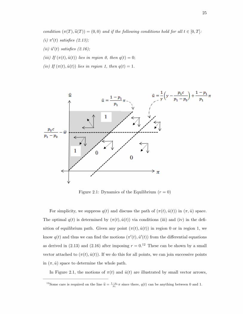
Below we define what an equilibrium path implies in terms of Figure 2.1.

Definition 4 A path (π(t), u(t), q(t)) is an equilibrium path if it satisfies the terminal

11The continuous time model has been derived by taking the limit ∆→ 0 in the discrete time model.Alternatively, one could start with the continuous time model and derive the same optimal contractusing continuous time dynamic programming.

25

condition (π(T ), u(T )) = (0, 0) and if the following conditions hold for all t ∈ [0, T ]:

(i) π′(t) satisfies (2.13);

(ii) u′(t) satisfies (2.16);

(iii) If (π(t), u(t)) lies in region 0, then q(t) = 0;

(iv) If (π(t), u(t)) lies in region 1, then q(t) = 1.

Figure 2.1: Dynamics of the Equilibrium (r = 0)

For simplicity, we suppress q(t) and discuss the path of (π(t), u(t)) in (π, u) space.

The optimal q(t) is determined by (π(t), u(t)) via conditions (iii) and (iv) in the defi-

nition of equilibrium path. Given any point (π(t), u(t)) in region 0 or in region 1, we

know q(t) and thus we can find the motions (π′(t), u′(t)) from the differential equations

as derived in (2.13) and (2.16) after imposing r = 0.12 These can be shown by a small

vector attached to (π(t), u(t)). If we do this for all points, we can join successive points

in (π, u) space to determine the whole path.

In Figure 2.1, the motions of π(t) and u(t) are illustrated by small vector arrows,

12Some care is required on the line u = 1−p1p1

π since there, q(t) can be anything between 0 and 1.

26

where a horizontal arrow points the direction of the motion of π(t) and a vertical

arrow points the direction of the motion of u(t). Then for region 0, i.e., below the line

u = 1−p1

p1π, the motions π′(t) and u′(t) are obtained by imposing q(t) = 0 into the

differential equations:

π′(t) = −y +p1c

p1 − p0

u′(t) = − p0c

p1 − p0+ ω

Assumptions 1 and 2 imply π′(t) < 0 and u′(t) < 0. Therefore both π(t) and u(t) are

decreasing in this region. Similarly in region 1, i.e., below the line u = 1−p1

p1π, the

motions are obtained by imposing q(t) = 1:

π′(t) = −y − γp1u(t) +p1c

p1 − p0+ γ(1− p1)π(t) (2.19)

u′(t) = − p0c

p1 − p0+ γu(t) + ω (2.20)

Equation (2.19) implies that the line

u =1

γ(y − p1c

p1 − p0) +

1− p1

p1π,

which is parallel to the line in equation (2.18), determines the direction of the motion of

π(t); above (below) it we have π′(t) < 0 (π′(t) > 0), i.e. π(t) is decreasing (increasing).

Observe that this line lies in region 0, which means that in region 1, π′(t) < 0 always

holds. The direction of the motion of u(t), however, is determined by the line

u =1

γ(

p0c

p1 − p0− ω).

Equation (2.20) implies u(t) is decreasing if u < 1γ ( p0c

p1−p0− ω), increasing otherwise.

Hence given any point (π(t), u(t)) in regions 0 or 1, the motion vectors of π(t) and

u(t) determine the subsequent change to proceed along the path passing through this

point. In Figure 2.1, we observe that given any point (π(t), u(t)), the motion of the path

27

is towards “south-east”, except when (π(t), u(t)) is in region 1 and u > 1γ ( p0c

p1−p0−ω). To

determine which paths could constitute an equilibrium, first recall that the equilibrium

path must satisfy the terminal condition. Therefore our equilibrium analysis requires

characterizing the paths which are convergent to the origin in Figure 2.1. This implies

that the path pointing to the “north-west” cannot be an equilibrium. Any path with

motion pointing at “south-east” is a candidate for an equilibrium unless it crosses to

region 1 when u > 1γ ( p0c

p1−p0− ω). Because in that case, it would not converge to the

origin.

With the help of phase diagram, we have studied the simplest case, r = 0. Now

we consider the case where r > 0. Let Π(t) ≡ e−rtπ(t) and U(t) ≡ e−rtu(t) denote

the present values of π and u. In (Π, U) space, the phase diagram (with r > 0) looks

exactly like Figure 2.1, simply replacing π by Π on the horizontal axis and u by U on the

vertical axis. See Figure 2.2. To see why this is true, first notice that U(t) = 1−p1

p1Π(t)

if and only if u(t) = 1−p1

p1π(t). Therefore, just as before, the line

U =1− p1

p1Π

separates Figure 2.2 into two regions, region 0 where q = 0 is optimal and region 1

where q = 1 is optimal. Second, when q = 0, the motions of u(t) and π(t) follow from

π′(t) = −y +p1c

p1 − p0+ rπ(t) (2.21)

u′(t) = − p0c

p1 − p0+ ω + ru(t)

These equations imply

Π′(t) = e−rt(π′(t)− rπ(t)

)= e−rt

(−y +

p1c

p1 − p0

)U ′(t) = e−rt

(u′(t)− ru(t)

)= e−rt

(− p0c

p1 − p0+ ω

)

Therefore,

Π′(t)

U ′(t)=π′(t)

u′(t)(2.22)

28

so the phase diagram in region 0 is exactly the same in Figure 2.2 as in Figure 2.1.

Similarly when q = 1, the motions of u(t) and π(t) follow from

u′(t) = − p0c

p1 − p0+ ω + (γ + r)u(t) (2.23)

π′(t) = −y − γp1u(t) +p1c

p1 − p0+ (r + γ(1− p1))π(t)

These equations imply

Π′(t) = e−rt(π′(t)− rπ(t)

)= e−rt

(−y − γp1u(t) +

p1c

p1 − p0+ γ(1− p1)π(t)

)U ′(t) = e−rt

(u′(t)− ru(t)

)= e−rt

(− p0c

p1 − p0+ ω + γu(t)

)

Therefore, (2.22) again holds: the phase diagram in region 1 in Figure 2.2 is identical

to the one in Figure 2.1.

Thus, the phase diagrams in Figure 2.1 (the case r = 0) and Figure 2.2 (the case

r > 0) are identical, except for the labelling of the axes. Clearly, the terminal condition

is also the same, (Π(T ), U(T )) = (0, 0).

The phase diagram analysis ruled out paths that do not converge to the origin.

However, it remains to characterize the equilibrium path. To complete our analysis,

in the next section, we derive the explicit equations of the paths and find necessary

conditions for a unique equilibrium path.

2.2.2 The Equilibrium Path: Main Theorem

In this section, using insights developed in the previous section, we investigate under

what conditions the equilibrium path lies in region i at t and whether it lies in a given

region for all t, or it crosses different regions over the contract horizon. We will show

that there always exists a unique equilibrium path, which characterizes the sequence of

optimal short-run contracts.

29

Figure 2.2: Dynamics of the Equilibrium (r > 0)

The optimal short-run contract optimally combines the two incentive tools, ter-

mination threat and success wage, and different circumstances will require different

combinations. Will the principal prefer to use a termination threat (a “stick”) or a

high success wage (a “carrot”) to provide incentives? From the agent’s point of view, a

termination threat provides only weak incentives if the agent does not expect to gain a

lot from the relationship in the future. But if the relationship gives the agent a payoff

which greatly exceeds her outside option, then the termination threat provides power-

ful incentives to work hard. From the principal’s point of view, the advantage of the

termination threat is that it stimulates effort even with a low success wage. In other

words, the principal can reduce the compensation costs when termination threat is an

available contracting tool. The drawback is that, if the agent is fired, the principal loses

his future gains from the relationship.

This reasoning suggests that whether or not a termination threat is optimal depends

on the relative sizes of the principal’s and the agent’s future gains. If the principal

expects to gain a lot from the relationship but the agent thinks the relationship is not

much better than her outside option, then the principal will not use a termination threat

30

(i.e. q = 0 at the optimum). If instead it is the agent who expects to gain a lot from the

relationship (compared to her outside option), then the principal will use a termination

threat (i.e. q = 1 at the optimum). More precisely, the key point is what fraction of the

surplus generated by the relationship goes to the agent and the principal, respectively.

This basic insight was already captured by Proposition 3. But Proposition 3 derived

the optimal firing rule as a function of the endogenously determined payoffs u(t) and

π(t). We will now consider how the optimal firing rule depends on the exogenously

given parameters of the model. For this, we need to know how u(t) and π(t) depend

on these parameters.

The principal’s and the agent’s payoffs in the dynamic relationship turn out to

be closely connected to their payoffs in a hypothetical one-shot game with the same

parameters as in our model. In the one-shot game, the principal gains y from high

effort, and pays a success wage cp1−p0

to provide incentives. The principal’s surplus

from this one-shot game would be

SP ≡ y −p1c

p1 − p0

while the agent’s surplus (net of outside option) would be

SA ≡p0c

p1 − p0− ω

The total one-shot surplus would be

S ≡ y − c− ω =

(y − p1c

p1 − p0

)︸ ︷︷ ︸

SP

+

(p0c

p1 − p0− ω

)︸ ︷︷ ︸

SA

(2.24)

Notice that S, SP and SA depend only on exogenously given parameters (y, c, p0, p1, ω).

It turns out that in our dynamic model, these one-shot surpluses play a key role. Define

K(T ) ≡ r + (1− p1)γ

r + γ

1− e−(r+γ)T

1− e−(r+(1−p1)γ)T(2.25)

31

It is shown in the next section that K(T ) < 1 for any T > 0. Our main result is the

following.

Theorem 5 (i) If

SA < (1− p1)S (2.26)

then q(t) = 0 and w′(t) = 0 for all t ∈ [0, T ]. (ii) If

SA >1− p1

K(T )S (2.27)

then q(t) = 1 and w′(t) > 0 for all t ∈ [0, T ]. (iii) If

(1− p1)S < SA <1− p1

K(T )S (2.28)

then there is t∗ > 0 such that 0 < q(t) < 1, q′(t) > 0 and w′(t) = 0 for t < t∗, and

q(t) = 1 and w′(t) > 0 for t > t∗.

The proof is in the next section, but here we provide an intuitive justification of

Theorem 5. It can be shown that (2.26) holds if and only if productivity y exceeds

some upper bound. Observe that in (2.10), it is only the principal’s payoff, π(t),

which depends on y, and π(t) is increasing in y. Since π(t) directly determines the cost

of imposing a termination threat, higher y means higher costs of termination threat.

Therefore, when productivity y is large enough, the cost of imposing threat outweighs its

benefit at all times, so optimality requires q(t) = 0 over the contract horizon. The best

incentive device to induce high effort in that case is wage compensation: the optimal

contract always pays the “efficiency wage” w(t) = c/γp1−p0

. Thus, if y is sufficiently high,

optimal contract is static in terms of both devices where it pays a constant stream

of wage combined with zero termination threat at all times. In other words, condition

(2.26) defines an upper bound for the agent’s share in total surplus: the optimal contract

never imposes a positive termination threat if the agent’s surplus in the one shot game

is sufficiently low.

It can also be shown that condition (2.27) holds if and only if productivity y is below

32

some lower bound. If y is sufficiently low, costs of imposing a termination threat are

low as compared to its benefits at all times. Then, at the optimum, the principal offers

q(t) = 1 over the entire contract horizon. From the IC condition, optimal wage is set

as low as possible at all times, w(t) = −u(t) + c/γp1−p0

. Observe that when (2.27) holds,

since u(t) is decreasing, optimal wage scheme is increasing through time: high effort

could be implemented only by a success wage which increases over time. The reason is

that as seniority increases, the agent’s loss from getting fired decreases. Then incentives

to work hard decreases through time. But termination threat cannot be adjusted to

the agent’s decreasing incentives simply because it is set at its maximum q(t) = 1 from

the beginning. Therefore the only way to provide stronger incentives is to offer higher

success wage as the agent gets older.

If condition (2.28) holds, productivity y is in a moderate range. Recall that π(t) is

the present value of future stream of profits from the relationship at time t. Therefore,

since π(t) determines the cost of imposing termination threat, we conclude that the

cost is decreasing as the contract approach to the end of horizon. When productivity

y is in a moderate range, costs are high at the start of contract horizon where the con-

tract offers relatively lower termination threat. However as we move in time, the cost

to the principal from losing his agent, decreases. Then the optimal contract gradually

increases the termination threat while it keeps offering a fixed success wage. Finally

the contract switches to severe threat regime when the costs from punishment decreases

significantly at a critical t∗. In the rest of contract horizon, severe threat regime ne-

cessitates increasing success wage profile in order to, as explained above, give sufficient

incentives to induce effort as the agent gets closer to the end of her career.

2.3 Proof of Theorem 5

We know that the optimal q(t) is determined by the sign of Ψ, defined in (2.10). The

evolution of Ψ is determined by

Ψ′(t) = p1u′(t)− (1− p1)π′(t) (2.29)

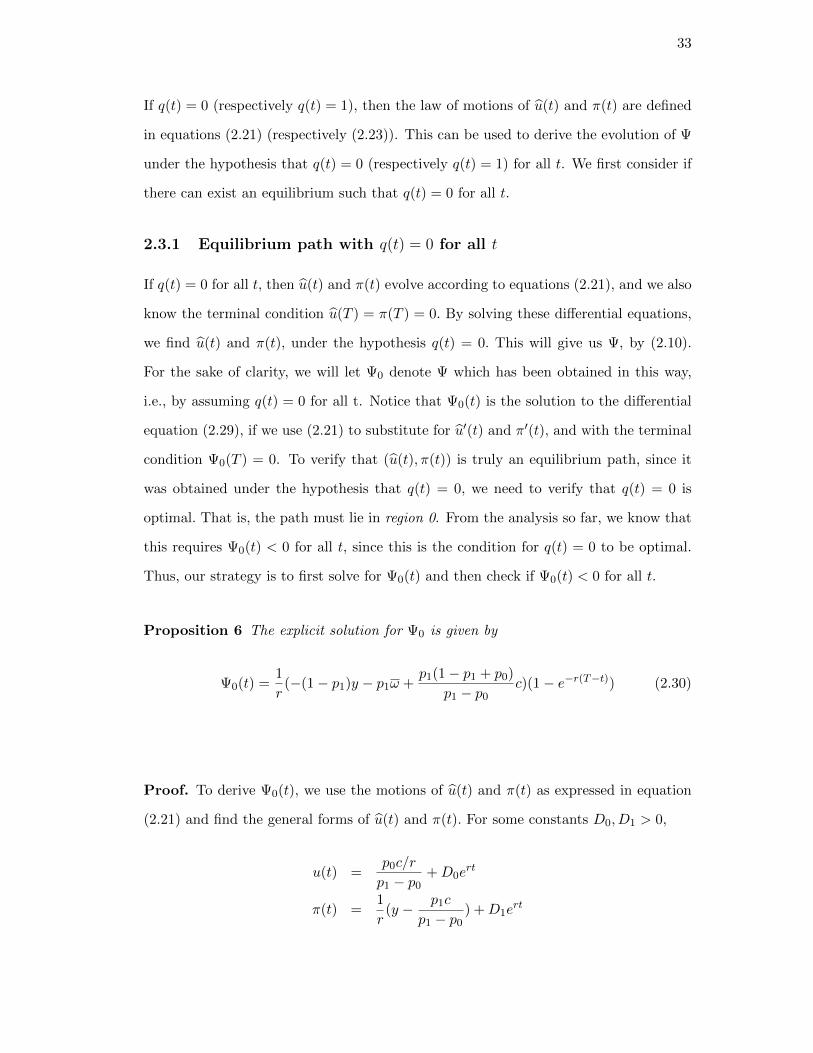
33

If q(t) = 0 (respectively q(t) = 1), then the law of motions of u(t) and π(t) are defined

in equations (2.21) (respectively (2.23)). This can be used to derive the evolution of Ψ

under the hypothesis that q(t) = 0 (respectively q(t) = 1) for all t. We first consider if

there can exist an equilibrium such that q(t) = 0 for all t.

2.3.1 Equilibrium path with q(t) = 0 for all t

If q(t) = 0 for all t, then u(t) and π(t) evolve according to equations (2.21), and we also

know the terminal condition u(T ) = π(T ) = 0. By solving these differential equations,

we find u(t) and π(t), under the hypothesis q(t) = 0. This will give us Ψ, by (2.10).

For the sake of clarity, we will let Ψ0 denote Ψ which has been obtained in this way,

i.e., by assuming q(t) = 0 for all t. Notice that Ψ0(t) is the solution to the differential

equation (2.29), if we use (2.21) to substitute for u′(t) and π′(t), and with the terminal

condition Ψ0(T ) = 0. To verify that (u(t), π(t)) is truly an equilibrium path, since it

was obtained under the hypothesis that q(t) = 0, we need to verify that q(t) = 0 is

optimal. That is, the path must lie in region 0. From the analysis so far, we know that

this requires Ψ0(t) < 0 for all t, since this is the condition for q(t) = 0 to be optimal.

Thus, our strategy is to first solve for Ψ0(t) and then check if Ψ0(t) < 0 for all t.

Proposition 6 The explicit solution for Ψ0 is given by

Ψ0(t) =1

r(−(1− p1)y − p1ω +

p1(1− p1 + p0)

p1 − p0c)(1− e−r(T−t)) (2.30)

Proof. To derive Ψ0(t), we use the motions of u(t) and π(t) as expressed in equation

(2.21) and find the general forms of u(t) and π(t). For some constants D0, D1 > 0,

u(t) =p0c/r

p1 − p0+D0e

rt

π(t) =1

r(y − p1c

p1 − p0) +D1e

rt

34

The terminal conditions u(T ) = π(T ) = 0 fixes D0 and D1:

D0 = − p0c/r

p1 − p0e−rT

D1 =1

r(y − p1c

p1 − p0)e−rT

Then

u(t) =1

r(

p0c

p1 − p0− ω)(1− e−r(T−t))

π(t) =1

r(y − p1c

p1 − p0)(1− e−r(T−t)

Therefore, using the above expressions for u(t) and π(t), we get Ψ0(t) :

Ψ0(t) = p1u(t)− (1− p1)π(t)

=1

r(−(1− p1)y − p1ω +

p1(1− p1 + p0)

p1 − p0c)(1− e−r(T−t))

Observe that by construction, we have Ψ0(T ) = 0. Also note that Ψ0(0) < 0, and

Ψ′0(t) > 0 for all t, if

p1(1− p1 + p0)

(1− p1)(p1 − p0)c− p1

1− p1ω < y (2.31)

Therefore, since Ψ0(T ) = 0, we conclude that Ψ0(t) < 0 for all t, i.e. the path

(u(t), π(t)) lies in region 0, if the condition in (2.31) holds. In Figure 2.3a this path

is illustrated with a solid path on the phase diagram. By construction, there cannot

be another such convergent path that always lies in region 0. Noticing that if (2.31)

holds, Ψ′′0(t) < 0 for all t, in Figure 2.3b we illustrate these findings for Ψ0(t) with a

solid curve. However if

y <p1(1− p1 + p0)

(1− p1)(p1 − p0)c− p1

1− p1ω

then Ψ0(0) > 0 and Ψ′0(t) < 0 for all t. These, together with Ψ0(T ) = 0 imply that

Ψ0(t) > 0 for all t; such path is illustrated with a dashed path in Figure 2.3a and with

35

a dashed path in Figure 2.3b. Recall that Ψ0(t) is derived under the assumption that

q(t) = 0 for all t. But Ψ0(t) > 0 means q(t) = 0 is not optimal, so this does not give us

an equilibrium path. In conclusion, when y is sufficiently high, i.e. when (2.31) holds,

we have found a unique equilibrium path as expressed in equation (2.30), which lies in

region 0 at all times.

Figure 2.3: Equilibrium Path with q(t) = 0 for all t

2.3.2 Equilibrium path with q(t) = 1 for all t

If q(t) = 1 for all t, then u(t) and π(t) evolve according to equations (2.23), and we also

know the terminal condition u(T ) = π(T ) = 0. By solving these differential equations,

we find u(t) and π(t), under the hypothesis q(t) = 1. This will give us Ψ, by (2.10).

For the sake of clarity, we will let Ψ1 denote Ψ which has been obtained in this way,

i.e., by assuming q(t) = 1 for all t. Notice that Ψ1(t) is the solution to the differential

equation (2.29), if we use (2.23) to substitute for u′(t) and π′(t), and with the terminal

36

condition Ψ1(T ) = 0. To verify that (u(t), π(t)) is truly an equilibrium path, we need

to verify that q(t) = 1 is optimal. That is, the path must lie in region 1. From the

analysis so far, we know that this requires Ψ1(t) > 0 for all t. Thus, our strategy is to

first solve for Ψ1(t) and then check if Ψ1(t) > 0 for all t.

Proposition 7 The explicit solution for Ψ1 is given by

Ψ1(t) =1

γ + r(

p0c

p1 − p0−ω)(1−e−(r+γ)(T−t))−(1− p1)(y − c− ω)

r + (1− p1)γ(1−e−(r+(1−p1)γ)(T−t))

(2.32)

Proof. To derive Ψ1(t) we use the of motions of u(t) and π(t) as defined by equation

(2.23)

u′(t) = − p0c

p1 − p0+ ω + (γ + r)u(t) (2.33)

π′(t) = −y − γp1u(t) +p1c

p1 − p0+ (r + γ(1− p1))π(t) (2.34)

Using equation (2.33), start with the general form, for some constant M0 > 0 :

u(t) =1

γ + r(

p0c

p1 − p0− ω) +M0e

(r+γ)t (2.35)

Then equation (2.34) becomes

π′(t) = −y − γp1

γ + r(

p0c

p1 − p0− ω)− γp1M0e

(r+γ)t +p1c

p1 − p0+ (r + γ(1− p1))π(t)

Therefore

π′(t)− (r + γ(1− p1))π(t) = −y − γp1

γ + r(

p0c

p1 − p0− ω) +

p1c

p1 − p0− γp1M0e

(r+γ)t

Then the form of π(t) can be derived by using the general form:

π(t) =1

r + (1− p1)γ(y +

γp1

γ + r(

p0c

p1 − p0− ω)− p1c

p1 − p0) +M0e

(r+γ)t +M1e(r+(1−p1)γ)t

(2.36)

37

where M0 and M1 are the constants to be determined. We first impose u(T ) = 0 in

equation (2.35) and get

M0 = − 1

γ + r(

p0c

p1 − p0− ω)e−(r+γ)T

Therefore the expression in equation (2.35) becomes

u(t) =1

γ + r(

p0c

p1 − p0− ω)(1− e−(r+γ)(T−t)) (2.37)

Using (2.37), the expression in (2.36) becomes

π(t) =1

r + (1− p1)γ(y +

γp1

γ + r(

p0c

p1 − p0− ω)− p1c

p1 − p0)−

1

γ + r(

p0c

p1 − p0− ω)e−(r+γ)(T−t) +M1e

(r+(1−p1)γ)t

Once again the terminal condition π(T ) = 0 fixes M1 :

M1 = (− 1

r + (1− p1)γ(y+

γp1

γ + r(

p0c

p1 − p0−ω)− p1c

p1 − p0)− 1

γ + r(

p0c

p1 − p0−ω))e−(r+(1−p1)γ)T

Finally, the expression for π(t) in equation (2.36) will be

π(t) =1− e−(r+(1−p1)γ)(T−t)

r + (1− p1)γ(y +

γp1

γ + r(

p0c

p1 − p0− ω)− p1c

p1 − p0)−

(e−(r+γ)(T−t) + e−(r+(1−p1)γ)(T−t))

γ + r(

p0c

p1 − p0− ω)

Then, after some simplifications, Ψ1(t) can be written as

Ψ1(t) = p1u(t)− (1− p1)π(t)

=1

γ + r(

p0c

p1 − p0− ω)(1− e−(r+γ)(T−t))− (1− p1)(y − c− ω)

r + (1− p1)γ(1− e−(r+(1−p1)γ)(T−t))

We will derive under what conditions Ψ1(t) > 0 is required for an equilibrium path

with q(t) = 1.

38

Recall that K(T ) was defined in equation (2.25). We need the following lemma.

Lemma 8 K(T ) < 1 for all T > 0.

Proof. Consider

K ′(T ) =(r + (1− p1)γ)e−(r+(1−p1)γ)T

(r + γ)(1− e−(r+(1−p1)γ)T )2((r + γ)e−γp1T − γp1e

−(r+γ)T − (r + (1− p1)γ))

It can be verified that

(r + γ)e−γp1T − γp1e−(r+γ)T − (r + (1− p1)γ) < 0

for all T > 0, because the expression is decreasing in T and equal to 0 at T = 0. Then

K ′(T ) < 0. Now observe that

1− e−(r+γ)T

1− e−(r+(1−p1)γ)T→ r + γ

r + (1− p1)γ

as T → 0. This implies K(T )→ 1 as T → 0. Therefore, since K ′(T ) < 0, we conclude

that K(T ) < 1 for all T > 0.

At this point, it is convenient to change variables and solve the differential equations

“backwards”. Therefore, let τ = T−t denote the time left before the horizon, and define

Φ(τ) ≡ Ψ1(T − τ). Explicitly,

Φ(τ) ≡ 1

γ + r(

p0c

p1 − p0− ω)(1− e−(r+γ)τ )− (1− p1)(y − c− ω)

r + (1− p1)γ(1− e−(r+(1−p1)γ)τ )

It turns out that, in order to check whether Ψ1(t) > 0 holds, a very convenient

method is to change variable from t to τ and study if it is true that Φ(τ) > 0. We need

a preliminary result.

Lemma 9 If τ∗ > 0 is such that Φ′(τ∗) = 0 then Φ′′(τ∗) < 0, hence there can exist at

most one such τ∗.

39

Proof. Differentiating, we find that

Φ′(τ) = (p0c

p1 − p0− ω)e−(r+γ)τ − (1− p1)(y − c− ω)e−(r+(1−p1)γ)τ

and

Φ′′(τ) = −[(r + γ)(

p0c

p1 − p0− ω)e−(r+γ)τ − (r + (1− p1)γ)(1− p1)(y − c− ω)e−(r+(1−p1)γ)τ

]

It follows that if Φ′(τ∗) = 0 then

Φ′′(τ∗) = −p1γ(p0c

p1 − p0− ω)e−(r+γ)τ < 0

Finally, Proposition 10 characterizes the conditions which determine the sign of

Φ(τ).

Proposition 10 (i) If

y < (K(T )p0

(1− p1) (p1 − p0)+ 1)c+ (1− K(T )

1− p1)ω (2.38)

then Φ(τ) > 0 for all τ ∈ [0, T ].

(ii) If

(K(T )p0

(1− p1) (p1 − p0)+ 1)c+ (1− K(T )

1− p1)ω < y <

p1(1− p1 + p0)

(1− p1)p1 − p0c− p1

1− p1ω (2.39)

then there exists τ∗ such that Φ(τ) > 0 for all τ ∈ [0, τ∗) and Φ(τ) < 0 for all τ ∈ (τ∗, T ].

(iii) If

y >p1(1− p1 + p0)

(1− p1)p1 − p0c− p1

1− p1ω (2.40)

then Φ(τ) < 0 for all τ ∈ [0, T ].

40

Proof. It can be checked that Φ(0) = 0, that Φ(T ) > 0 is equivalent to (2.38), and

that Φ′(0) > 0 is equivalent to

y <p1(1− p1 + p0)

(1− p1)p1 − p0c− p1

1− p1ω (2.41)

(i) Notice that (2.38) implies (2.41) by Lemma 8. Hence, if (2.38) holds, then

Φ(0) = 0, Φ′(0) > 0 and Φ(T ) > 0. Now Lemma 9 implies Φ(τ) > 0 for all τ ∈ [0, T ].

(ii) If (2.39) holds, then Φ(0) = 0, Φ′(0) > 0 and Φ(T ) < 0. Now Lemma 9 implies

there exists τ∗ such that Φ(τ) > 0 for all τ ∈ [0, τ∗) and Φ(τ) < 0 for all τ ∈ (τ∗, T ].

(iii) Notice that (2.40) implies (2.38) is violated, by Lemma 8. Hence, if (2.40)

holds, then Φ(0) = 0, Φ′(0) < 0 and Φ(T ) < 0. Now Lemma 9 implies Φ(τ) < 0 for all

τ ∈ [0, T ].

Since t = T − τ and Φ(τ) ≡ Ψ1(T − τ), it directly follows from Proposition 10 that

Ψ1(t) > 0 for all t if (2.38) holds but Ψ1(t) < 0 for all t if (2.40) holds. However if

(2.39) holds, there exists t∗ ≡ T − τ∗ such that Ψ1(t) < 0 for all t < t∗, and Ψ1(t) > 0

for all t > t∗. So we have found another equilibrium path, which lies in region 1 at

all times as far as (2.38) holds. In Figure 2.4a this is illustrated with a solid path on

the phase diagram. Using Lemma 9, in Figure 2.4b, we summarize our findings for

Ψ1(t) with a solid curve. By construction, there cannot be another such convergent

path that always lies in region 1. Indeed, notice that (2.40) is equivalent to (2.31),

which implies if (2.38) holds, (2.31) is violated; i.e. Ψ0(t) cannot give an equilibrium

with q(t) = 0. Similarly, if (2.40) holds, hence (2.38) is violated, Ψ1(t) does not give

an equilibrium with q(t) = 1, and as we have previously verified q(t) = 0 for all t is the

unique equilibrium path in that case.

2.3.3 “Mixed” equilibrium path

For the intermediate case where (2.39) holds, i.e. both (2.38) and (2.31) are violated,

Proposition 10 suggests that there always exists t∗ ∈ (0, T ) where Ψ1(t) < 0 for all

t < t∗, and Ψ1(t) > 0 for all t > t∗. Figure 2.5b illustrates Ψ1(t) for this case. When

(2.39) holds, (2.31) is violated, then Ψ0(t) can never give an equilibrium with q(t) = 0.

41

Figure 2.4: Equilibrium Path with q(t) = 1 for all t

But Ψ1(t) > 0 for all t > t∗, Ψ1(t) is the unique equilibrium path for that time interval.

However, it cannot give an equilibrium with q(t) = 1 for t < t∗ since Ψ1(t) < 0 in

that interval. Then the equilibrium path must satisfy Ψ(t) = 0 for all t < t∗, i.e. the

equilibrium path lies on the line u = (1−p1)p1

π as illustrated in Figure 2.5b.

To find critical point in time, t∗, at which the optimal contract imposes a termination

threat, we directly solve Ψ1(t∗) = 0 : since we solve for the equilibrium backwards and

given that at the end of the contract horizon Ψ1(t) is optimal if (2.39) holds, it suffices

to find where Ψ1(t) > 0 no longer holds. Then equilibrium t∗ follows from

Ψ1(t∗) =1

γ + r(

p0c

p1 − p0−ω)(1−e−(r+γ)(T−t∗))−(1− p1)(y − c− ω)

r + (1− p1)γ(1−e−(r+(1−p1)γ)(T−t∗)) = 0

(2.42)

For future reference, the agent’s and principal’s payoffs at this critical t∗ are com-

puted using (2.37) and (2.36):

42

u(t∗) =1

γ + r(

p0c

p1 − p0− ω)(1− e−(r+γ)(T−t∗)) (2.43)

π(t∗) =1− e−(r+(1−p1)γ)(T−t∗)

r + (1− p1)γ(y +

γp1

γ + r(

p0c

p1 − p0− ω)− p1c

p1 − p0)

(e−(r+γ)(T−t∗) + e−(r+(1−p1)γ)(T−t∗))

γ + r(

p0c

p1 − p0− ω)

Figure 2.5: ”Mixed” Equilibrium Path

Optimal Firing Rule for the “Mixed” Equilibrium

We showed that condition (2.39) produces a mixed equilibrium which requires Ψ(t) = 0

for all t < t∗ and Ψ(t) = Ψ1(t) for all t > t∗. Therefore, towards the end of horizon, the

equilibrium path behaves exactly the same as the equilibrium path we derived in the

previous section. The interesting part of the mixed equilibrium is that it requires Ψ(t) =

43

0 for t < t∗. From (2.17) where we derived the optimal firing rule: q(t) ∈ [0, 1] if Ψ(t) =

0. In this case, any q(t) could be optimal, but we show in Proposition 11 that there

is a unique q(t) consistent with an equilibrium path. It also states the optimal wage

and agent’s continuation payoff on this time interval. Since the termination threat also

determines optimal success wage and continuation payoffs in equilibrium, Proposition

11 also provides equilibrium paths of w(t) and u(t).

Proposition 11 If Ψ(t) = 0, for all t ≤ t∗

(i) optimal firing rule is

q(t) =1

γu(t)(−1− p1

p1y +

1− p1 + p0

p1 − p0c− ω) (2.44)

where q(t) increases on the interval (0, q(t∗))

(ii) optimal wage is

w =1

γ(1− p1

p1y + ω + c) (2.45)

(iii) agent’s continuation payoff follows

u(t) =1− p1

rp1(y − p1c

p1 − p0)(1− e−r(t∗−t)) + u(t∗)e−r(t

∗−t)) (2.46)

where t∗ solves (2.42) and u(t∗) is defined in (2.43).

Proof. (i) Since Ψ(t) = 0 corresponds to u(t) = (1−p1)p1

π(t), we have

du(t)

dπ(t)=

1− p1

p1(2.47)

Using (2.13) and (2.16), (2.47) becomes

q(t)u(t) =1

γ(−1− p1

p1y +

1− p1 + p0

p1 − p0c− ω) (2.48)

Therefore (2.48) must hold when Ψ(t) = 0 in equilibrium. Since, whatever the func-

tional form in equilibrium is, we know that u(t) is decreasing in t. Then keeping q(t)u(t)

constant to satisfy the condition (2.48) for all t ≤ t∗ implies that optimal q(t) must

44

increase on this time interval. Therefore q(t∗) is the highest optimal threat for t < t∗ .

To find q(t∗), use u(t∗), as calculated in (2.43), and equation (2.48). Then

q(t∗) =

1γ (−1−p1

p1y + 1−p1+p0

p1−p0c− ω)

1γ+r ( p0c

p1−p0− ω)(1− e−(r+γ)(T−t∗))

(2.49)

(ii) From IC constraint, in equation (2.11), and optimal firing rule, as defined in equation

(2.48), optimal w(t) is in fact a constant:

w =1

γ(1− p1

p1y + ω + c)

(iii) Using the optimal constant wage w, optimal firing rule in equation (2.48), and the

motion of the equilibrium continuation payoff of the agent as defined in equation (2.4),

we can derive equilibrium u(t). For some constant N0 > 0, we use the general form

u(t) =1− p1

rp1(y − p1

p1 − p0) +N0e

rt

To determine N0, we use u(t∗), in (2.43), as a terminal condition.

N0 = (u(t∗)− 1− p1

rp1(y − p1

p1 − p0))e−rt

∗

Therefore

u(t) =1− p1

rp1(y − p1c

p1 − p0)(1− e−r(t∗−t)) + u(t∗)e−r(t

∗−t)

Hence there is an increasing termination threat on the time interval [0, t∗] where

q(t) ∈ (0, q(t∗)). After critical t∗, the maximum threat regime will be optimal, i.e.

q(t) = 1 for all t > t∗. Since on the line, u(t) = (1−p1)p1

π(t), condition (2.48) must

hold and productivity y is constant, this means right hand side of the condition is also

constant. Therefore left hand side being constant implies that from (2.11), a fixed

wage will be optimal. Thus the optimal contract increases probability of firing while

compensating the agent with a flat wage upto critical t∗ : since the agent’s incentive’s to

45

work hard decreases as she gets more senior, the only way to adjust optimal incentives on

this interval is to increase punishment. But after t∗, a fixed wage along with increasing

termination threat profile is not sustainable, to give the sufficient incentives the optimal

contract switches to increasing wage scheme along with maximum termination threat

in the rest of horizon. Lemma 12 shows that optimal termination threat at critical t∗

is in fact strictly less than 1.

Lemma 12 q(t∗) < 1.

Proof. First observe that Ψ1(t) is upward-sloping at t = t∗ :

Ψ′1(t∗) = −(p0c

p1 − p0−ω)e−(r+γ)(T−t∗)+(1−p1)(y−c−ω)e−(r+(1−p1)γ)(T−t∗) > 0 (2.50)

Inequality (2.50) is equivalent to

( p0cp1−p0

− ω)

r + (1− p1)γe−(r+γ)(T−t∗) − (1− p1)(y − c− ω)

r + (1− p1)γe−(r+(1−p1)γ)(T−t∗) < 0 (2.51)

At t∗ we have

Ψ1(t∗) =1

γ + r(

p0c

p1 − p0−ω)(1−e−(r+γ)(T−t∗))−(1− p1)(y − c− ω)

r + (1− p1)γ(1−e−(r+(1−p1)γ)(T−t∗)) = 0

(2.52)

Adding (2.51) and (2.52):

[( p0cp1−p0

− ω)

r + (1− p1)γe−(r+γ)(T−t∗) − (1− p1)(y − c− ω)

r + (1− p1)γe−(r+(1−p1)γ)(T−t∗)

]+[

1

γ + r(

p0c

p1 − p0− ω)(1− e−(r+γ)(T−t∗))− (1− p1)(y − c− ω)

r + (1− p1)γe−(r+(1−p1)γ)(T−t∗)

]< 0

This can be simplified as follows:

1

γ + r

(p0c

p1 − p0− ω

)e−(r+γ)(T−t∗) <

(1− p1)

p1γ(y−c−ω)− (r + (1− p1)γ)

(γ + r) p1γ(

p0c

p1 − p0−ω)

(2.53)

46

But (2.53) implies

1

γ + r(

p0c

p1 − p0− ω)(1− e−(r+γ)(T−t∗)) >

1

γ + r(

p0c

p1 − p0− ω)− (1− p1)

p1γ(y − c− ω)

+(r + (1− p1)γ)

(γ + r) p1γ(

p0c

p1 − p0− ω)

=1

γ

(−1− p1

p1y +

1− p1 + p0

p1 − p0c− ω

)

Therefore, q(t∗) < 1.

2.3.4 Summary of the analysis

Consider Ψ(t) as defined by (2.10). The above equilibrium analysis can be summarized

as follows:

Ψ(t) =

Ψ1(t) if y < ( K(T )p0

(1−p1)(p1−p0) + 1)c+ (1− K(T )1−p1

)ω

0 for t ≤ t∗ and Ψ1(t) for t > t∗ if( K(T )p0

(1−p1)(p1−p0) + 1)c+ (1− K(T )1−p1

)ω < y

< p1(1−p1+p0)(1−p1)(p1−p0)c−

p1

1−p1ω

Ψ0(t) if y > p1(1−p1+p0)(1−p1)(p1−p0)c−

p1

1−p1

Corresponding to Ψ(t), we get the following termination threat over the contract

horizon:

q(t) =

1 if y < ( K(T )p0

(1−p1)(p1−p0) + 1)c+ (1− K(T )1−p1

)ω

∈ (0, q(t∗)) for t ≤ t∗ and 1 for t > t∗ if

( K(T )p0

(1−p1)(p1−p0) + 1)c+ (1− K(T )1−p1

)ω

< y

< p1(1−p1+p0)(1−p1)(p1−p0)c−

p1

1−p1ω

0 if y > p1(1−p1+p0)(1−p1)(p1−p0)c−

p1

1−p1

Once optimal q(t) is determined, optimal wage contract directly follows from the IC

47

constraint, expressed in equation (2.11). Specifically,

w(t) =

c/γp1−p0

if q(t) = 0

−u(t) + c/γp1−p0

if q(t) = 1

1γ (1−p1

p1y + ω + c) if q(t) ∈ (0, 1)

(2.54)

The following proposition summarizes our findings so far.

Proposition 13 The equilibrium path satisfies,

(i) If

y < (K(T )p0

(1− p1) (p1 − p0)+ 1)c+ (1− K(T )

1− p1)ω (2.55)

then

w(t) = −u(t) +c/γ

p1 − p0

and q(t) = 1 for all t ∈ [0, T ], where u(t) is defined in (2.37).

(ii) If

(K(T )p0

(1− p1) (p1 − p0)+ 1)c+ (1− K(T )

1− p1)ω < y <

p1(1− p1 + p0)

(1− p1)(p1 − p0)c− p1

1− p1ω (2.56)

then for t ≤ t∗ we have

w(t) =1

γ(1− p1

p1y + ω + c)

and

q(t) =1

γu(t)(−(

1− p1

p1y + ω) +

1− p1 + p0

p1 − p0c)

where u(t) follows (2.46) and t∗ solves (2.42); while for t > t∗ we have

w(t) = −u(t) +c/γ

p1 − p0

and q(t) = 1, where u(t) is defined in (2.37).

(iii) If

y >p1(1− p1 + p0)

(1− p1)(p1 − p0)c− p1

1− p1ω (2.57)

48

then w(t) = c/γp1−p0

and q(t) = 0 for all t ∈ [0, T ].

Figure 2.6 illustrates the optimal contract. Panels [a], [b] and [c] correspond to the

cases in part (i), part (ii) and part (iii) of Proposition refContract2, respectively, where

we illustrate the equilibrium path, termination threat and success wage for each case.

In each panel, on the top we illustrate the equilibrium path, Ψ(t) for a given range of

productivity y. Given the equilibrium path on the top, the middle and lower rows show

the components of the optimal q(t) and w(t), respectively.

Now we can complete the proof of Theorem 5. It is easy to check that the condition

(2.31), which determines the cutoff for the punishment-free contract, can be rewritten

as (2.26). If agent’s productivity is sufficiently high, or agent’s surplus in the one-

shot game is sufficiently low, the optimal contract does not use termination threat at

all. Therefore, the incentives to induce effort can only be provided by a high success

wage through the contract horizon. Condition (2.38) can be re-expressed as condition

(2.27), which defines a lower bound for the agent’s expected surplus: the contract

always imposes severe termination threat at all times if the agent’s surplus in one shot

game is not too low. But from (2.54) optimal wage is set as low as possible at every

instant: −u(t) + c/γp1−p0

. As explained before, success wage is upward sloping since as

the agent’s tenure increases, her incentives to work hard decreases: her expected loss

in case of failure, p1u(t), decreases. Hence the optimal incentives must be stronger

as the agent gets more senior. Finally, the intermediate “mixed” case corresponds to

condition (2.28). If productivity is in a moderate range, the optimal contract offers

an increasing termination threat scheme, combined with a constant wage stream in

the early phase of time horizon, which would be replaced by an increasing wage profile

after critical t∗. As we verified previously, q(t∗) < 1, i.e. termination threat profile has a

jump at t∗. For that reason, after t∗, success wage decreases for a limited time interval:

w = q(t∗)u(t∗) + c/γp1−p0

> −u(t∗) + c/γp1−p0

, as illustrated in panel [b] below. But this

follows an increasing wage scheme until the end of time horizon. At the end of contract

horizon, optimal wage certainly exceeds w since w(T ) = c/γp1−p0

> 1γ (1−p1

p1y+ω+ c) > w,

by condition (2.28).

49

Figure 2.6: The Optimal Contract

50

2.4 Comparative Dynamics

In this section, we focus on how the change of parameters affect the nature of the

equilibrium path. We are mainly interested in the changes in quality differential of

agent’s output, i.e. YH − YL; success probability when low effort is exerted, i.e. p0;

and discount rate, r. Observe from equation (2.1), where we define y, that a change

in quality differential on agent’s output, YH − YL, is in fact equivalent to a change in

agent’s productivity, holding γ(p1− p0) constant. The parameter p0 (the probability of

succeeding without trying) can be thought of as a measure of “luck”, and r is a measure

of impatience.

2.4.1 A change in quality differential

It is straightforward to see the effect of a change in YH−YL on the optimal termination

threat. Consider the lower and upper bounds for productivity y in Proposition 13.

Since they are independent from the quality differential, it is easy to track how optimal

q(t) responds to a given change in the differential: as quality differential increases,

termination threat (weakly) decreases. Below we verify this impact and also evaluate

the change in w(t) and illustrate how these results in fact follow from the impact on

the equilibrium path in Figure 2.6.

To see the argument let us start assuming YH − YL, and hence y, is relatively low

initially: y = y0 such that (2.55) holds. Denoting the optimal contract by (w0(t), q0(t))

when y = y0, we get

(w0(t); q0(t)) = (−u0(t) + c/γ(p1 − p0); 1), ∀t ∈ [0, T ) (2.58)

From equation (2.32), clearly ∂Ψ1(t)/∂y < 0; i.e. as y increases, Ψ1(t) shifts down in

a fashion as illustrated in panel [a] of Figure 2.7.13 If the increase in y is sufficiently

low such that (2.55) still holds, Ψ1(t) shifts down a little bit. Therefore the optimal

13From equation (2.32), we get Ψ′1(T ) = − p0cp1−p0

+ ω + (1− p1)(y − c− ω). Condition (2.55) implies

Ψ′1(T ) < 0. As y increases such that (2.55) still holds, Ψ′1(T ) gets less negative, i.e the function becomesflatter around T.

51

contract is still given in (2.58). Now suppose y increases to y = y1 > y0 such that

(2.55) is violated but (2.56) holds. In other words, Ψ1(t) shifts down so we move to

panel [b]. From the previous analysis, we know that if (2.56) holds, there exits t∗1 such

that Ψ1(t∗1) = 0. Then the equilibrium path becomes:

(w1(t), q1(t)) =

(w1; 1γu1(t)(−(1−p1

p1y1 + ω) + 1−p1+p0

p1−p0c)), ∀t ∈ [0, t∗1]

(−u1(t) + c/γp1−p0

; 1), ∀t ∈ (t∗1, T )(2.59)

where w1 = 1γ (1−p1

p1y1 +ω+ c). A comparison of (2.58) and (2.59) leads to the following

result.

Lemma 14 q1(t) ≤ q0(t) but w1(t) ≥ w0(t) for all t.

Proof. Obviously q1(t) = q0(t) for all t ∈ (t∗1, T ). Recall from Lemma 12 and Proposi-

tion 11 that q1(t∗1) < 1 and q1(t) < q1(t∗1), ∀t ∈ [0, t∗1]. Therefore, q1(t) < q0(t) = 1 for all

t ∈ [0, t∗1]. Finally, we consider how w(t) changes. First note that on (t∗1, T ), u(t) follows

from (2.37) since q = 1 on this interval. Then −u1(t) = −u0(t), i.e. w1(t) = w0(t) for all

t ∈ (t∗1, T ). Also, from our previous analysis, we know that w1 > −u1(t∗1)+c/γ(p1−p0).

This implies w1 > −u0(t∗1) + c/γ(p1 − p0) = w0(t∗1). Since w0(t∗1) > w0(t) for all t < t∗1,

we conclude that w1 > w0(t). Therefore w1(t) ≥ w0(t) for all t.

Now suppose y increases to y = y2 > y1 such that (2.56) still holds. From the

previous analysis, there exists t∗2 such that Ψ1(t∗2) = 0. But since Ψ1(t) keeps shifting

down as illustrated in panel [b], t∗2 > t∗1. Then the new equilibrium path is:

(w2(t), q2(t)) =

(w2; 1γu2(t)(−(1−p1

p1y2 + ω) + 1−p1+p0

p1−p0c)), ∀t ∈ [0, t∗2]

(−u2(t) + c/γp1−p0

; 1), ∀t ∈ (t∗2, T )(2.60)

where w2 = 1γ (1−p1

p1y2 + ω + c).

Lemma 15 q2(t) ≤ q1(t) but w2(t) ≥ w1(t) for all t.

52

Proof. It is easy to check that q(t) weakly decreases for all t ∈ (t∗1, T ) : even though

q2(t) = q1(t) for all t ∈ (t∗2, T ), q2(t) < q1(t) for all t ∈ (t∗1, t∗2] by the same argument that

we used above; the regime where q < 1 replaces q = 1 regime over this time interval.

Obviously, agent’s payoff is decreasing in q(t). Since q2(t) ≤ q1(t) for all t ∈ (t∗1, T ),

then u2(t∗1) > u1(t∗1). This means, from (2.49), q2(t∗1) < q1(t∗1) < 1. This, together with

q2(t) < q2(t∗1) for all [0, t∗1] (since q(t) must be upward sloping on [0, t∗2]) implies that

q2(t) < q1(t) for all t ∈ [0, t∗1]. To evaluate the impact on success wage, observe that

u1(t) = u2(t) for all t ∈ (t∗2, T ). Then w1(t) = w2(t) for all t ∈ (t∗2, T ). But for all t ∈

(t∗1, t∗2], w2 > w1(t): since

w2 > −u2(t∗2) +c/γ

p1 − p0= −u1(t∗2) +

c/γ

p1 − p0> −u1(t∗1) +

c/γ

p1 − p0= w1(t).

Therefore we conclude that w2(t) ≥ w1(t).

Finally suppose y increases to y = y3 > y2 such that (2.56) is violated and (2.57)

holds. In other words, Ψ1(t) shifts down significantly where Ψ1(t) < 0 for all t. Then

Ψ1 becomes irrelevant as we move to panel [c]. The new equilibrium path is:

(w3(t); q3(t)) = ( c/γp1−p0

; 0), ∀t ∈ [0, T )

Lemma 16 q3(t) < q2(t) and w3(t) > w2(t) for all t.

Proof. The decrease in optimal threat is clear. We also observe that c/γp1−p0

>

maxw2,−u2(t) + c/γp1−p0

for all t. In other words, w3(t) > w2(t) for all t.

Combining Lemmas 14, 15 and 16 yields the following result:

Theorem 17 As the agent’s productivity increases, holding γ(p1−p0) constant, the ter-

mination threat (weakly) decreases, whereas the success wage (weakly) increases. When

it is defined, the critical t∗ increases.

Summarizing this analysis, we have found that the two contracting devices respond

to an increase in quality differential in opposite ways: the termination threat decreases

53

while wage incentives increase. One straightforward intuition is that the instantaneous

net benefit from punishment, i.e. p1u(t)− (1 − p1)π(t), decreases as productivity y

increases. The principal does not want to lose her agent as his productivity increases,

so she lowers the punishment level. At the same time, she increases the success wage

to induce high effort. A similar intuition follows from our previous argument with

one-shot surpluses. An increase in y holding γ(p1− p0) constant is equivalent to, using

(2.24), an increase in SP while SA is constant, and hence an increase in S. Therefore, as

agent’s share from the total surplus in one-shot game decreases, the termination threat

becomes less useful.

54

Figure 2.7: A Change in Quality Differential

55

2.4.2 A change in luck

To see the impact on the optimal contract with respect to p0, we start with p0 = p00

such that (2.57) holds. We will gradually increase p0 and consider how the contract in

Figure 2.6 changes.

When (2.57) holds, Ψ0(t) < 0 for all t < T . Therefore there is never any termination

threat over the horizon. In panel [c] of Figure 2.8, the optimal contract is illustrated

with black lines. Denote the equilibrium path when p0 = p00 by (w0(t), q0(t)):

(w0(t); q0(t)) = (−u0(t) + c/γ(p1 − p00); 0), ∀t ∈ [0, T )

Note that right hand side of the inequality in (2.57) is increasing but left hand side

is decreasing in p0. Therefore as p0 increases, (2.57) will eventually be violated. We also

observe that ∂Ψ0(t)/∂p0 > 0: the function moves up, keeping the end point constant,

as p0 increases. For sufficiently small increase in p0, Ψ0(t) moves up a little and (2.57)

still holds. In panel [c], we illustrate this impact. Hence q(t) does not change. But

since c/γp1−p0

is increasing in p0, w(t) shifts up as we show in panel [c].

Now let p0 = p10 > p0

0, such that (2.57) is violated but (2.56) holds. In that case,

Ψ0(t) > 0 for all t so Ψ0 becomes irrelevant. From Proposition 13, there exists a critical

t∗1 and the equilibrium path is as illustrated in panel [b]. Denote the optimal contract

when p0 = p10 by (w1(t), q1(t)). Then we have:

(w1(t), q1(t)) =

(w1; 1γu1(t)(−(1−p1

p1y(p1

0) + ω) +1−p1+p1

0

p1−p10c)) ∀t ∈ [0, t∗1]

(−u1(t) + c/γp1−p1

0; 1), ∀t ∈ (t∗1, T )

(2.61)

where w1 = 1γ (1−p1

p1y(p1

0) + ω + c). Therefore q(t) increases for all t, while the success

wage, w(t), decreases at all times. That is:

Lemma 18 q0(t) < q1(t) and w0(t) > w1(t) for all t.

Now assume a further increase in the luck parameter: p0 = p20 > p1

0 such that

(2.56) still holds and we again have mixed equilibrium where there exists t∗2 such that

56

Ψ1(t∗2) = 0. The optimal contract changes in the following way:

(w2(t), q2(t)) =

(w2; 1γu2(t)(−(1−p1

p1y(p2

0) + ω) +1−p1+p2

0

p1−p20c)) t ∈ [0, t∗2]

(−u2(t) + c/γp1−p2

0; 1) ∀t ∈ (t∗2, T )

(2.62)

where w2 = 1γ (1−p1

p1y(p2

0)+ω+c). To see how the equilibrium path in panel [b] changes,

observe that ∂Ψ1(t)/∂p0 > 0 and ∂Ψ′1(T )/∂p0 > 0 .14 Then Ψ1(t) shifts up in the

illustrated fashion. This verifies that t∗2 < t∗1. In other words, the optimal contract enters

the maximum termination-threat regime at an earlier point in time as p0 increases: the

agent will be exposed to the highest threat for a longer time interval at the end her

career. Now we compare (2.61) and (2.62).

Lemma 19 q2(t) ≥ q1(t) for all t.

Proof. Clearly, q2(t) = q1(t) for all t ∈ (t∗1, T ). But q1(t) < q1(t∗1) < 1 = q2(t) for

all t ∈ [t∗2, t∗1]. To see the impact on [0, t∗2), we need to evaluate how optimal q(t), as

defined in (2.44), changes. Observe that ∂y/∂p0 < 0 and since u(t) follows from (2.46),

∂u(t)∂p0 < 0. Then ∂q(t)/∂p0 > 0 so q2(t) > q1(t) for all t ∈ [0, t∗2).This impact is

illustrated in panel [b].15

Next, we compare w1(t) and w2(t) in (2.61) and (2.62). First note that −u(t) +

c/γ(p1− p0) is increasing in p0.16 Then w2(t) > w1(t) for all t ∈ (t∗1, T ). However, since

14Since ∂y∂p0

< 0,

∂Ψ1(t)

∂p0=

p1c

(p1 − p0)2(γ + r)(1− e−(r+γ)(T−t))− (1− p1)

r + (1− p1)γ(1− e−(r+(1−p1)γ)(T−t))

∂y

∂p0> 0

15It is easy to check that ∂2q(t)/∂p0∂t > 0 in that interval, i.e termination scheme gets steeper asillustrated in panel [b].

16Directly follows from:

∂(−u(t) + c/γ(p1 − p0))/∂p0 =c

(p1 − p0)2(− p1

γ + r(1− e−(r+γ)(T−t)) +

1

γ)

>c

(p1 − p0)2(− p1

γ + r+

1

γ) > 0

57

∂w/∂p0 < 0, w2(t) < w1(t) for all t ∈ [0, t∗2). But the impact on w(t) over the interval

(t∗2, t∗1) is unclear.17 Nevertheless, the comparison of (w1(t), q1(t)) and (w2(t), q2(t))

yields the following conclusion: whenever the optimal contract cannot adjust q(t) to

an increase in p0 further (i.e. on the interval (t∗1, T ) where the threat was already set

at the highest possible value), then high effort could be induced only with higher w(t).

However if q(t) could be adjusted to an increase in p0 (i.e. on the interval [0, t∗2)), then

cost minimizing contract decreases w(t).

Finally let p0 = p30 > p2

0 such that (2.56) is violated but (2.55) holds. Then Ψ1(t) > 0

for all t and we have panel [a] in Figure 2.8. Then the optimal contract is

(w3(t), q3(t)) = (−u3(t) + c/γ(p1 − p30), 1);∀t ∈ [0, T ]

Obviously, q(t) weakly increases. Thus, we have:

Lemma 20 q3(t) = q2(t) for all [t∗2, T ), and q3(t) > q2(t) for all t ∈ [0, t∗2).

As p0 keeps increasing, (2.55) still holds, i.e. Ψ1(t) shifts up as illustrated in panel

[a]. Therefore q(t) does not change. But since −u(t) + c/γ(p1 − p0) is increasing in p0,

w(t) shifts up as illustrated.18 Hence w(t) increases at all times. Again, we have the

same result: whenever it is not possible to adjust the optimal incentives via an increase

q(t), with respect to an increase in p0, the optimal adjustment on the contract is to

increase w(t).

Theorem 21 As the luck parameter p0 increases, the termination threat (weakly) in-

creases. When it is defined, the critical t∗ decreases.

It is also possible to show that ∂2u(t)/∂p0∂t > 0, i.e the upward sloping part of the wage schemegets steeper as p0 increases.

17Over the time interval [t∗2, t∗1], the relationship between w2(t) and w1 is not clear. In panel [b],

we illustrated a small shift in the increasing portion of the wage scheme: w2(t) < w1 for all [t∗2, t∗1].

However if there is a larger shift, it would be possible to have w2(t) > w1 for t ∈ [t∗3, t∗1], but w2(t) < w1

for all t ∈ [t∗2, t∗3]. It cannot be possible to have a huge shift such that w2(t) > w1 for all t ∈ [t∗2, t

∗1] :

w2 > w2(t) at least for some [t∗2, t∗2 + ε]; and w1 > w2. Therefore w1 > w2(t) holds at least over a small

interval.

18Again since ∂2u(t)/∂p0∂t > 0, the wage scheme gets steeper when p0 increases, as depicted in panel[a].

58

Summarizing, the termination threat is always increasing in p0. Intuitively, as luck

becomes more important, the incentives must be stronger to encourage effort, and

the principal raises the termination threat. Again, in terms of one-shot surpluses, we

observe from equation (2.24) that as p0 increases, the agent’s share from the total

surplus increases: SA increases as S decreases. Hence, the firing option becomes more

attractive. We also showed critical t∗ also increases as p0 gets larger; i.e. the agent will

be exposed to the maximum termination threat for a longer time interval.

Even though our analysis suggests that the impact on the optimal wage is not clear,

for some cases, we have been able to show that if the principal can increase termination

threat, as a response to an increase in p0, optimal wage decreases. If the termination

threat is already set at the maximum level, or the increase in p0 is not enough to push

productivity y down to a moderate range, then the principal does not have the option

to adjust the termination threat. For such cases, the success wage is adjusted instead:

higher p0 increases the optimal success wage to provide stronger incentives to work

hard.

59

Figure 2.8: A Change in Luck

60

2.4.3 A change in discount rate

Finally, we consider how a change in r affects the equilibrium path. In this section, we

do a partial analysis: first we will show how the optimal contract responds to a change

in r when productivity (i.e., y) takes relatively high values (i.e. when (2.57) holds).

Then we consider what happens when productivity is in a moderate range (i.e. when

(2.56) holds) and finally when it takes relatively low values (i.e. when (2.55) holds).

a. High productivity

Suppose condition (2.57) holds. In this case, If y is high enough so that the optimal

contract does not use any termination threat. It is straightforward to see that the

optimal q(t) is constant with respect to a change in r, because condition (2.57) does

not depend on r. Observe from Proposition 13 that, when (2.57) holds, w(t) does not

depend on r either. The only impact is on Ψ0(t), that is derived in (2.30). Note that

the sign of Ψ0(t) does not depend on r. In panel [c] of Figure 2.9, we illustrate the

impact on Ψ0(t).19

Theorem 22 If condition (2.57) holds, then the success wage increases as r increases.

b. Moderate productivity

Suppose r increases from r1 to r2 > r1, and suppose condition (2.56) holds both before

and after the increase. We know from previous analysis that when (2.56) holds, there

exists a mixed equilibrium where the path enters a maximum termination-threat regime

at a critical t∗. Denote the corresponding critical point in time and the optimal contract

when r = ri by t∗i and (wi(t), qi(t)), respectively. Then when r = r1, the equilibrium

19It can be checked that 1−e−r(T−t)

ris decreasing in r .This implies, since (2.57) holds, Ψ0(t) increases,

i.e., it shifts up, as r increases. But (2.57) implies that Ψ0(t) < 0 will always holds regardless of themagnitude of the increase in r.

61

path is

(w1(t), q1(t)) =

(w1; 1γu1(t)(−(1−p1

p1y + ω) + 1−p1+p0

p1−p0c)); t ∈ [0, t∗1]

(−u1(t) + c/γp1−p0

; 1); ∀t ∈ (t∗1, T )(2.63)

where w1 = 1γ (1−p1

p1y + ω + c). When r = r2, the equilibrium path is

(w2(t), q2(t)) =

(w1; 1γu2(t)(−(1−p1

p1y + ω) + 1−p1+p0

p1−p0c)); t ∈ [0, t∗2]

(−u2(t) + c/γp1−p0

; 1); ∀t ∈ (t∗2, T )(2.64)

where w2 = 1γ (1−p1

p1y + ω + c).

We first show that the critical time increases as r increases: t∗2 > t∗1. In other words,

the time interval where agent is exposed to maximum termination threat gets larger.

Lemma 23 t∗2 > t∗1.

Proof. Define

z(θ) ≡ (p0c

p1 − p0−ω)(

((r + γ)θ + 1)e−(r+γ)θ − 1

(r + γ)2−((r + γ(1− p1))θ + 1)e−(r+γ(1−p1))θ − 1

(r + (1− p1)γ)2)

(2.65)

Claim: z(θ) > 0 for all θ > 0.

To prove this claim, consider

z′(θ) = (p0c

p1 − p0− ω)θ(−e−(r+γ)θ + e−(r+γ(1−p1))θ) > 0

Since z(0) = 0, then z(θ) > 0 for all θ > 0. This proves the claim.

Now consider

∂Ψ1(t∗)

∂r= (

p0c

p1 − p0− ω)

((r + γ)(T − t∗) + 1)e−(r+γ)(T−t∗) − 1

(r + γ)2−

(1− p1)(y − c− ω)((r + γ(1− p1))(T − t∗) + 1)e−(r+γ(1−p1))(T−t∗) − 1

(r + (1− p1)γ)2

62

Let θ = T − t∗ > 0. Then (2.56) implies

∂Ψ1(t∗)

∂r> (

p0c

p1 − p0− ω)[

((r + γ)(T − t∗) + 1)e−(r+γ)(T−t∗) − 1

(r + γ)2

−((r + γ(1− p1))θ + 1)e−(r+γ(1−p1))(T−t∗) − 1

(r + (1− p1)γ)2]

= z(T − t∗) > 0

where the final inequality uses the claim.

Using (2.42) and the Implicit Function Theorem, we have

∂t∗

∂r= − ∂Ψ1(t∗)/∂r

∂Ψ1(t∗)/∂t∗

Since ∂Ψ1(t∗)/∂t∗ > 0 and ∂Ψ1(t∗)/∂r > 0 we conclude that ∂t∗

∂r < 0. Therefore t∗2 < t∗1.

We will show that the termination threat is weakly increasing in r. First we need a

few preliminary results.

Definition 24 Define

Ω(T ) ≡ ((T − t)(γ + r) + 1)e−(γ+r)(T−t∗) − 1)

and

Λ(t∗) ≡ ((T − t)(γ + r) + 1)e−(γ+r)(T−t∗) − (γ + r)(t∗ − t)− 1

(γ + r)2

Lemma 25 Ω(T ) < 0 for all T > 0.

Proof. Ω′(T ) = −(γ + r)2e−(γ+r)(T−t∗)(T − t) < 0. Since Ω(0) = 0, Ω′(T ) < 0 implies

Ω(T ) < 0 for all T > 0.

Lemma 26 Λ(t∗) > 0, ∀t∗ < T.

Proof. Λ′(t∗) = Ω(T )γ+r . By Lemma 25 , Λ′(t∗) < 0. Also since Λ(T ) = 0, we conclude

that Λ(t∗) > 0 for all t∗ < T.

63

Note that qi(t) depends on the agent’s continuation payoff ui(t), as defined in (2.46).

We prove that u(t) is decreasing in r.

Lemma 27 ∂u(t)∂r < 0, where u(t) is defined in (2.46).

Proof. Using (2.46), we get

∂u(t)

∂r= −1− p1

r2p1(y − p1c

p1 − p0)(1− e−r(t∗−t)) + (2.66)

1− p1

rp1(y − p1c

p1 − p0)(t∗ − t)e−r(t∗−t)∂t

∗

∂r+ (

∂u(t∗)

∂r− u(t∗)(t∗ − t))∂t

∗

∂re−r(t

∗−t))

Since ∂t∗

∂r < 0, the second term in equation (2.66) is negative. In the last term, we have:

∂u(t∗)

∂r− u(t∗)(t∗ − t)

=1

(γ + r)2[((T − t∗)(γ + r) + 1)e−(r+γ)(T−t∗) − 1− (γ + r)(t∗ − t)e−(r+γ)(T−t∗)]

=((T − t)(γ + r) + 1)e−(γ+r)(T−t∗) − (γ + r)(t∗ − t)− 1

(γ + r)2

From Lemma 26, this expression is positive. This proves that the last term in equation

(2.66) is negative. Therefore we conclude that ∂u(t)∂r < 0.

We are finally ready to prove that the termination threat increases.

Proposition 28 q2(t) ≥ q1(t).

Proof. Observe that for all t ∈ [0, t∗2], q1(t) = q2(t). Also for all t ∈ (t∗2, t∗1], q1(t) < q2(t)

since q1(t) < 1 but q2(t) = 1 on this time interval. Finally, since by Lemma 27,

u2(t) < u1(t), we conclude that q2(t) > q1(t) for all t ∈ [0, t∗2]. Therefore, q2(t) ≥ q1(t).

Unfortunately, we do not have an unambiguous result ofor w(t). Consider w1(t) and

w2(t) in (4.28) and (4.34). Observe that w1(t) = w2(t) for all t ∈ [0, t∗2].But for all

t ∈ (t∗1, t∗2), the relationship between w1(t) and w2(t) is again unclear20. Finally, to

20For the time interval [t∗2, t∗1], the relationship between w2(t) and w1 is not clear. This is again

64

compare w1(t) and w2(t) over the time interval (t∗1, T ), we determine how u(t), which

is derived in (2.37), changes as r changes:

∂u(t)

∂r= (

p0c

p1 − p0− ω)

((T − t)(γ + r) + 1)e−(r+γ)(T−t) − 1

(γ + r)2(2.67)

Since

∂u(t)

∂r= (

p0c

p1 − p0− ω)

Ω(T )

(γ + r)2,

by Lemma 25, we conclude that ∂u(t)∂r < 0. Then u2(t) < −u1(t), i.e. w2(t) > w1(t).

We summarize the discussion:

Theorem 29 As long as condition (2.56) holds, the termination threat (weakly) in-

creases, and the critical t∗ decreases, as r increases.

c. Low productivity

If (2.55) holds, Ψ1(t) > 0 for all t. Therefore severe threat is optimal over the entire

horizon. The impact over the equilibrium path Ψ1(t) can be found by considering:

∂Ψ1(t)

∂r= (

p0c

p1 − p0− ω)

((r + γ)T + 1)e−(r+γ)(T−t) − 1

(r + γ)2

−(1− p1)(y − c− ω)((r + γ(1− p1))(T − t) + 1)e−(r+γ(1−p1))(T−t) − 1

(r + (1− p1)γ)2

> (p0c

p1 − p0− ω)(

((r + γ)(T − t) + 1)e−(r+γ)(T−t) − 1

(r + γ)2

−((r + γ(1− p1))θ + 1)e−(r+γ(1−p1))(T−t) − 1

(r + (1− p1)γ)2)

where the last inequality follows from the observation that (2.56) implies (2.57). Now

let θ = T − t in (2.65). Then the last line in the above inequality is z(T − t). Since we

have verified in the proof of Lemma 23 that z(.) > 0, this implies ∂Ψ1(t)∂r > 0.

because of the same reason we explained in the note 2.4.2. In panel [b], we illustrate a small shift inthe upward sloping of the wage scheme: w2(t) < w1 for all [t∗2, t

∗1]. However if there is a larger shift,

it would be possible to have w2(t) > w1 for t ∈ [t∗3, t∗1], but w2(t) < w1 for all t ∈ [t∗2, t

∗3]. It cannot

be possible to have a huge shift such that w2(t) > w1 for all t ∈ [t∗2, t∗1] : w2 > w2(t) at least for some

[t∗2, t∗2 + ε]; and w1 = w2. Therefore w1 > w2(t) holds at least over a small interval.

65

Therefore, as r increases, Ψ1(t) shifts up in a fashion as illustrated in panel [a] and

the condition in (2.55) continues to hold. In other words, given that y is sufficiently

low, severe threat will still be optimal at all times as r increases. But since, from

(2.67), ∂u(t)/∂r < 0, the wage profile will shift up as depicted in panel [a].: optimal

w(t) increases at all times. Thus, we have the following:

Theorem 30 If condition (2.55) holds, then the success wage increases as r increases.

d. Summary of the effect of a change in r

The threat of termination always (weakly) increases as r increases. For the cases where

the termination threat strictly increases, the intuition is that as the future becomes less

important, the present value of the loss from getting fired decreases on the agent’s side,

i.e. incentives to work hard gets weaker. Therefore, the principal increases the threat,

in order to induce high effort. However, if the principal does not have the opportunity

to make such adjustment on the optimal threat because the threat is already maximal,

then she offers higher wages to induce high effort as r increases.

66

Figure 2.9: A Change in Discount Rate

67

2.5 Concluding Comments

Lazear (1979) showed that an increasing wage-schedule is the solution to the dynamic

moral hazard problem when the principal can commit to a long-run contract. This

important result explained real life practices including the frequent use of mandatory

retirement policies. In contrast, we have studied the dynamics of alternative incentive

tools in a moral hazard model with a fixed contract horizon when the principal’s com-

mitment ability is limited. We found conditions under which a termination threat is

optimal. As in Lazear’s model, the optimal incentives, in terms of both termination

threat and performance wage, get stronger as the agent gets more senior. In particular,

we obtain an upward sloping wage profile, even though the principal offers a sequence

of short-run contracts.

Performance based firing is a common practise. In our model, the termination

threat reduces the need for a performance based wage, and will be an efficient device

under particular conditions. Specifically, the principal will use a termination threat

if the agent expects a significant surplus from the relationship, relative to what the

principal expects. The termination threat is more likely to be optimal when the agent’s

probability of success when shirking increases, or as the interest rate increases. However

the termination threat is less desirable as the agent gets more productive. In that case,

incentive provision is achieved by higher performance pay.

68

Chapter 3

Incentivizing CEOs via Pay and Forced Turnover: Do

Tenure and Managerial Ability Matter?

3.1 Introduction

Boards, senior management teams, and shareholders are constantly struggling to design

the right type of executive compensation plans. This is a typical agency problem: the

executive (the agent) must be motivated to act in the best interests of the shareholders

(the principals), who have delegated their authority to the board of directors. The the-

oretical principal-agent literature has mainly focused on the use of performance-related

pay as an incentive device. However, incentives can also be provided by the threat

of termination of employment following poor performance. These two instruments in-

teract: a termination threat provides good incentives only if the expected future pay

within the firm is significantly higher than the outside option.

As Lazear (1981) argues, principal-agent theory predicts that wages should increase

with tenure to provide good incentives. On the other hand, it is less clear whether the

optimal termination threat will also be increasing, i.e., if poor performance is more likely

to result in termination for senior than for junior executives. Moreover, as Lazear’s

(1981) upward sloping wage schedule causes the senior executive’s compensation to

exceed her marginal product, the principal has the incentive to fire her even if she

behaves well. Therefore, Lazear’s (1981) optimal contract must involve a long-run

commitment to not fire the executive unless her performance is bad. However, long-term

contracts are not common in CEO labour markets; performance is mostly evaluated

annually and contracts are renewed every year.

69

In Olcay (2012), I consider a dynamic principal-agent model with limited commit-

ment to study the optimal contracts with incentive pay and termination threat. Even

though the model is designed to study the incentive pay (i.e. pay-performance sen-

sitivity), due its simplifying assumptions, the interpretation of its results regarding

incentive pay is applicable to the total pay as well. The model predicts that the use

of both incentive devices, incentive pay and termination threat, increases with tenure.

A termination threat is included in the short-term contract if and only if the agent’s

expected future surplus from the relationship is sufficiently high compared to the princi-

pal’s expected future gain. Moreover, at a given point in time, the observed productivity

(”ability”) of the agent affects the optimal use of the two incentive devices in opposite

ways. The higher is the agent’s ability, the higher should be the wage conditional on

good performance, and the smaller should be the risk of termination conditional on bad

performance.

The focus of our empirical study is first, to which extend pay and forced turnover are

used as incentive devices for CEOs; second, whether there is a significant relationship

of job tenure and managerial ability to these devices. We also consider how ability

and tenure interact in the provision of incentives: does managerial ability influence the

sensitivities of CEO pay and forced turnover to tenure?

Several previous theories also have implications for the relationships between tenure,

managerial ability, and the two incentive devices, as well as tenure and ability impacts

on the performance sensitivities of these devices. The most prominent are the learning

theory of Murphy (1986), the carrer concerns model of Gibbons and Murphy (1992),

and the entrenchment theory of Hermalin and Weisbach (1998). Table 3.1 summarizes

the predictions of these theories. We start with discussing the predictions of each theory

regarding the relationships of tenure with the two incentive devices.

Murphy (1986) proposes an adverse selection model where the executive’s ability is

not known to the shareholders. Then the optimal contract should be designed to fa-

cilitate the shareholder’s learning about the executive’s ability. First, pay-performance

sensitivity decreases as the CEO’s tenure increases: it is optimal to offer a contract

70

which is more sensitive to performance during the early years of tenure when the share-

holders have a only a little information about the CEO’s ability. As time passes, the

need to tie pay directly to performance decreases as the shareholders learns more about

the true ability by observing and assessing the CEO’s performance. Second, as beliefs

about ability are updated through time, pay level increases. Murphy (1986) does not

provide direct predictions for the probability of forced turnover.

Gibbons and Murphy’s (1992) model also has adverse selection, where a new CEO’s

true ability may not be perfectly known, and limited commitment. However, unlike

Murphy (1986), the presence of a competitive executive market creates “career con-

cerns” for the young executive whose true ability is not known. Therefore, in the early

years of her tenure, the risk-averse executive is motivated to work hard to establish her

reputation, but, at the same time, is reluctant to bear too much risk. This results in

relatively a lower pay-performance sensitivity as compared to later years in her tenure

where both board need to offset the reduction in her career concerns and risk-sharing

becomes easier.

The adverse selection model in Gibbons and Murphy (1992) helps us to derive

conclusions regarding the effect of performance on the likelihood of forced turnover.

As Allgood and Fareel (2000) point out, since a board has high uncertainty about

the CEO’s ability at the start of her tenure, the board is less willing to punish when

performance falls below the expected level. However, through time, learning leads to a

decrease in the variance of expected performance and hence a performance that would

not have triggered termination earlier may do so later. In other words, the impact of

performance on the probability of forced turnover increases through tenure.

The entrenchment theory of Hermalin and Weisbach (1998) differs dramatically from

standard principal-agent theories of optimal contracting. Not surprisingly, it produces

quite different predictions about the relationship between tenure and the two incentive

tools. If the executive gets more entrenched and dominates the board as she gets senior

in her tenure, the board’s ability to fire her in case of poor performance decreases.

Moreover, the entrenched manager who dominates the board can in effect set her own

71

pay, and can make it less sensitive to firm performance (Bebchuk and Fried, 2004).

Under the entrenchment theory, the longer the executive serves, the more entrenched

she becomes, resulting in not only a higher level of pay and lower pay-performance

sensitivity, but also in a lower likelihood of forced turnover and weaker performance-

forced turnover relationship.

Regarding the relationship between managerial ability and incentive provision, the

career concerns and entrenchment theories also present essential insights. In terms of

explicit incentives, in the form of total pay, and ability, Gibbons and Murphy’s (1992)

career concerns theory makes an intuitive prediction. Since higher profits reveal good

news about her ability, a CEO may negotiate for a raise after strong profits if she

has enough bargaining power in the board. In this way, the CEO can capture the

whole surplus created by the good news. But if low profits reveal bad news about the

CEO’s ability, the board may want to negotiate for a lower level of CEO pay. However,

if the CEO has enough bargaining power in the presence of long-term contract, the

shareholders have to bear the full negative surplus from bad news. A formalization

of this perspective by Harris and Holmstrom (1982) suggests that when a CEO has

enough bargaining power, shareholders suffer more from bad news about the CEO’s

ability than they benefit from good news. The entrenchment theory (Bebchuk, Fried,

and Walker (2002) and Bebchuk and Fried (2003)) would explain the positive ability-

pay relationship again by higher ability CEOs being more likely to get entrenched and

increase their own pay. An alternative explanation is provided by a competitive talent

assignment model of Gabaix and Landier (2008) suggesting that the most skilled CEOs

are matched with the largest firms and earn the highest salaries.

Regarding the likelihood of forced turnover, in a career concerns model, since it

relies on learning, a negative relationship between performance related turnover and

ability arises: highly talented CEOs are identified as those whose performance is less

uncertain and thereby less likely to be informative. Therefore, higher ability is associ-

ated with weaker performance-forced turnover relationship. Similarly, highly talented

72

CEOs would be immune to performance-related dismissals according to the entrench-

ment model (Bebchuk, Fried, and Walker (2002) and Bebchuk and Fried (2003)): CEOs

of higher abilities are identified as more powerful and hence more likely to face a pas-

sive board of directors. In other words, for a higher ability and hence more entrenched

CEO, probability of forced turnover is both weaker and less sensitive to performance.

To summarize, a number of theories have predicted a positive relationship between

explicit incentives in the form of total compensation and tenure. The impact of tenure

on the relationship between pay and performance is positive in carreer concerns model

and Olcay (2012), but negative in learning and entrenchment models. Ability, on

the other hand, effects total pay positively in all models. However, it affects pay-

performance relationship negatively in entrenchment model whereas in Olcay (2012)

it has the opposite impact. In terms of probability of forced turnover, tenure has a

positive impact in Olcay (2012), negative impact in entrenchment model. Sensitivity

of this device to performance is, however, positive in both carrer concerns and Olcay

(2012), but negative in entrenchment model. On the other hand, all theories agree

on their predictions concerning adverse impact of ability on the probability of forced

turnover and its performance sensitivity. In Sections 3.3 and 3.4, we investigate these

hypotheses empirically. The current theories provide no specific prediction on whether

and how managerial ability affects tenure sensitivities of CEO pay and likelihood of

CEO turnover, but I also explore this issue empirically. Future research on executive

contract design may shed light on this issue from a theoretical perspective.

The empirical analysis in this paper is two fold. Analysis-I, in Section 3.3, focuses

on CEO pay as an incentive tool in executive contracting and analyzes how it changes

through tenure and managerial ability. The analysis of pay-to-performance sensitivity is

left for future research. Analysis-II, in Section 3.4, concentrates on forced CEO turnover

due to bad performance, and investigates how the use of this incentive device depends

on tenure and managerial ability. Two empirical proxies for managerial ability are used:

media visibility, which attempts to capture reputational aspects of the “outsider” CEO’s

ability and is hand-collected through counting articles in top business journals; and the

73

age when the “insider” CEO is promoted to the position. The idea is that higher media

visibility and lower age at the time of promotion are both signals of higher managerial

ability. Data on executive compensation, firm performance and control variables, both

at the CEO and firm level, is drawn from the COMPUSTAT database. Data for forced

turnover is hand-collected by reading news items which are found through Factiva and

Google web search. The sample used in Analysis-I contains a larger data set with all

firms in S&P 1500 (i.e. S&P 500-LargeCap, S&P 400- MidCap and S&P 600-SmallCap)

between 1998-2008, except when the ability proxy is media visibility which is created

only for firms in the S&P 500- LargeCap for the same period. The sample used in

Analysis-II, however, is smaller and includes firms only in S&P 500-LargeCap over the

period 1998-2008.

My empirical results suggest that CEO performance and the two devices; i.e. pay

and threat of forced turnover, are stongly connected. In other words, these tools are

indeed used as incentive mechanisms. Also, I find that, as they are more senior, CEOs

receive higher pay. However, there is no support for whether the likelihood of forced

turnover changes through a CEO’s tenure. For outsider CEOs, reputation, as a measure

for managerial ability, is shown to increase pay where the impact is strongest as more

current reputational measures are used. At the same time, it decreases tenure sensi-

tivity of pay only when it is proxied by the most current (i.e. short-term) reputational

measure. As an alternative incentive tool for CEOs, the likelihood of forced turnover

is decreasing in managerial ability where ability is proxied by age-at-promotion for in-

siders and by reputation for outsiders. Reputation is also found to a weaker impact on

forced turnover as it measures by less current measures.

The existing empirical literature on the determinants of executive pay is large and we

cannot give a full review here. Early studies concentrated on the relationship between

CEO pay and company performance (Coughlan and Schmidt (1985), Murphy (1985,

1986), Jensen and Murphy (1990), Abowd (1990), Leonard (1990)). These articles show

that firm performance is largely positively related to pay-performance sensitivity after

controlling for risk. Others studies are focused on whether CEOs are rewarded for

74

performance which is measured relative to the market or industry (Antle and Smith

(1986), Gibbons and Murphy (1990)).

A growing literature studies company financial performance following CEO turnover.

An important early finding as noted by Coughlan and Schmidt (1985) and Warner,

Watts and Wruck (1988), is that a firm’s net of market performance and the probabil-

ity of turnover are inversely associated. However, these studies document that managers

are rarely fired due to poor performance even though the negative relationship between

stock price performance and turnover following bad performance has generally been in-

terpreted as evidence that boards fire poorly performing CEOs. Later research provides

evidence for turnover rates that have become more sensitive to performance (Huson,

Parrino and Starks 1998). This leads to the idea that termination, as an incentive tool,

is becoming more important threat over the top executives.

A related finding by Weisbach (1988) is that the magnitude of the turnover-performance

relation is strongest in companies dominated by independent outside directors. Parrino

(1997), in an attempt to confirm the common use of relative performance evaluation

for top executives, shows that the outside replacements are mostly used by the compa-

nies which perform relatively poorly as compared their peers. These studies indicate

that poor firm performance is the single most important determinant of involuntary

turnover.

Another line of empirical research diregards the theoretical implications of opti-

mal contract design, and instead studies the relationship between forced turnover and

the entrenchment effect of top managers’ equity ownership. Murphy and Zimmerman

(1993), Huson, Parrino, and Starks (2001), Denis, Denis, and Sarin (1997) and Hadlock

and Lumer (1997), Goyal and Park (2002) and Dahya, Lonie, and Power (1998) inves-

tigate the impact of corporate governance on performance-turnover relationship. The

probability of top executive turnover is found to be negatively related to the ownership

stake of officers and directors. For example, Dahya, Lonie, and Power (1998) report

that forced top management turnover is more frequent for executives who own less than

1% of their firms’ equity.

75

The paper proceeds as follows. Section 3.2 describes the data sources and variables.

Sections 3.3 and 3.4 present the empirical tests and results regarding pay and forced

turnover, respectively. Section 3.5 concludes.

3.2 Data Description

In order to analyze the impact of CEO tenure and managerial ability on pay and the

likelihood of forced turnover, I construct a dataset of the CEO labour market which

contains detailed information on CEO turnovers. The dataset also includes empirical

proxies for CEO ability. In this section, I explain how the dataset is constructed and

the collection process for each of the variables used in this paper.

3.2.1 Sample Selection

The CEO succession data is hand-collected and includes all firms in S&P 500-LargeCap

for the period, 1998-2008. ExecuComp provides information on the five top executives

of all firms in the S&P 1500 (S&P LargeCap, S&P MidCap and S&P SmallCap).

I recognize a turnover for each year in which the CEO is identified in ExecuComp

changes.1

To identify forced departure, I carefully search news items on the Lexis-Nexis Aca-

demic Universe and Factiva, for each CEO change. Changes accompanied by poor

performance are identified as forced turnover. These news items openly state that the

prior stock price or accounting returns have been declining in the past quarters. Also

for each succession in the sample, I hand collect exact announcement dates which are

the earliest dates of the news about incumbent CEO departure and successor CEO

appointment. All other news which explicitly mention that CEO has departed the

company because she became a CEO at another firm, forced out for different reasons

(for example improper use of corporate funds, violation of Security Exchange Act, etc.),

resigned due to conflict with board, left due to health reasons, deceased or retired are

1To identify turnover, Parrino (1997), Huson, Parrino, and Stark (2001), Huson, Malatesta, andParrino (2004), use Forbes surveys. Jenter and Kanaan (2006) also use ExecuComp for the period1993-2001.

76

not included. My method of identifying turnover is similar to that of Weisbach (1988),

Denis and Denis (1995).

By using news items, I form different categories for reasons of CEO departure.

Table 3.2 gives information about the number of CEO departures for different reasons

during 1998-2008. The sample consists of 542 CEO changes out of 4769 firm-year

observations during 1998-2008. The total turnover rate is 11.4%.2 Using this detailed

information regarding CEO turnover as summarized in Table 3.1, I construct the forced

turnover data in Table 3.5. Forced 1 is constructed using the news items in which it

is explicitly stated that the CEO is terminated for poor performance. This yields 105

CEO changes. For the rest of classification I follow Parrino’s (1997) method. Such

classification is important in a study of forced CEO turnover since CEOs are seldomly

fired openly due to poor performance. I classify the remaining changes as “potential

forced departure” if the departing CEO is less than the normal retirement age which is

the mean age for CEO departure. In our sample, this is around age 61. In Table 3.5,

Forced 2 includes CEO changes if the reason of departure is announced either as retired

(but excluding those announcements which explicitly state that the departure is not

related with performance), or if the reason is not specified, or the news item specifies the

departure as unexpected or abrupt, and for all these observations the CEO is below the

normal retirement age. This yields 107 more observations for forced turnover. Forced

3 is the sum of Forced 1 and Forced 2.

In Table 3.2, 39% of all CEO changes are performance related. This finding is in line

with a total forced turnover rate of 36%, as found by Milbourn (2009) whose sample

covers 1993-2005 and firms in S&P 1500. However, the total forced turnover rate in

our sample is relatively higher than the one reported by Huson, Parrino, and Starks

(2001) who found a forced turnover rate of 23.4% for the sample of executives listed in

Forbes only and over the period 1989-1994. Table 3.2, however, reveals that while the

turnover data in the sample at hand does not show a particular time pattern, there is

significant time variation both in the rate of forced turnover and in the rate of overall

2This is consistent with previous studies, 12.2% (Parrino1997), 9.3% (Denis et al. 1997).

77

turnovers.

3.2.2 Measures for Firm Performance and Firm Level Controls

I enhance the dataset with several measures of firm operating performance, in addition

to various firm level controls which have been identified as important measures in the

CEO labour market. All measures listed on this section are at calendar year-end.

Descriptive statistics for these variables are summarized in Table 3.4.

I mainly use three different measures of firm performance all of which are provided

by COMPUSTAT: return on assets (ROA), return on equity (ROE) and ratio of Net

Income to the book value of assets (NIA). For each of the performance measure, I

create industry average counterparts. This helps to filter out industry specific shocks

in the analysis of forced turnover. In the COMPUSTAT database, each firm has been

specified with a four-digit SIC code. To identify the industry, I use the first two digits

of the SIC code. By using the overall sample in COMPUSTAT (over 20,000 firms), I

calculate industry averages for the firms in the sample at hand.

The main set of firm controls includes firm size (logarithm of total assets) and

firm’s dividend yield. All measures for these variables are taken from COMPUSTAT.

As discussed by the previous studies (for example Gabaix and Landier (2008) and Tervio

(2007)), firm size is an important variable on CEO labour markets. The dividend yield

of the firm is used to control for a firm’s riskiness.

3.2.3 CEO Pay, Tenure and CEO Characteristics

In order to examine the effect of tenure on a CEO’s level of pay, I use the natural

logarithm of the dollar value of CEO’s total pay (ExecuComp’s TDC1). This is defined

as the sum of salary, bonus, long-term incentive plans, restricted stock, and stock

appreciation rights.

Previous research suggests that CEO pay is a function of CEO age (see, for example,

Milbourn (2003) and Chevalier and Ellison (1999). Therefore age is included as a

control variable in the analysis. Data for CEO tenure is created by using data items in

78

Execucomp. Finally, I classify CEOs who had been with their firms for one year or less

at the time of their appointments as outsiders. 3As Table 3.4 summarizes, the median

CEO in our sample has 5 years of tenure, is 55 years old and has been promoted from

inside.

3.2.4 Measures for CEO’s power on Corporate Governance

To control for CEO’s potential power on corporate governance, which might have a sig-

nificant impact on pay level and likelihood of turnover, there are two different variables

used in the analysis. Using data items in ExecuComp, I create two dummy variables:

Board Member is equal to 1 if the CEO has served as a director during the calendar

year, and Share Ownership is equal to 1 if the CEO holds more than 5% of the firm’s

total shares. Table 3.4 indicates that 3 % of the whole sample contain firm-year obser-

vations with the firm’s CEO holding either 5 % or more of the total shares. Also 97%

of the firm-year observations, contain CEOs who are a board member.

3.2.5 Measures for CEO Ability

I construct three different empirical proxies for CEO ability. The first two proxies are

based on the number of articles in which the CEO’s name and company affiliation

appear in major US and global newspapers and business journals in a given calendar

year. The third proxy uses the age of the CEO at the time of promotion. Below we

discuss each in detail.

The first empirical proxy, Press, measures the media visibility of a CEO and at-

tempts to capture how the CEO’s ability is perceived. To create Press variable, I count

the number of articles containing the CEO’s name and company affiliation that appear

in the major business newspapers. A list of these sources is listed in the Appendix B.

A similar proxy is previously used by Milbourn (2003), Francis, Huang, Rajgopal and

Zang (2004), and Rajgopal, Shevlin, and Zamora (2006)). However, since “reputation”,

3ExecuComp has missing observations for the data item “Date Joined the Company” which deter-mines whether the CEO is an outsider. For the sample at hand, it has only been possible to categorize5915 (out of 11804) of the observations in our sample.

79

as implied by Press variable builds in time, I extend this proxy further and create three

different proxies out of it: Press (1year), Press (3years) and Press (5years) refer to the

number of articles during the previous year, last three years, and last five years prior

to the current year. For example, in year 2005, Press (1 year) shows the article counts

in year 2004, Press (3 years) shows the count between 2002-2004, finally Press (5years)

between 1999-2004. With this extension, media visibility measures reputation in dif-

ferent terms; Press (1 year) refers to a relatively more current measure of reputation

whereas Press (5 years) is a proxy for less current measure of reputation.

Using Lexis-Nexis database and restricting the search to the list of firms in Appendix

B, I conduct text searches using both the CEO’s last name and company name. The

classification of media visibility variable uses the same methods as previously used by

Milbourn (2003), Francis, Huang, Rajgopal and Zang (2004), and Rajgopal, Shevlin,

and Zamora (2006)): CEOs with higher media visibility are more likely to be of higher

ability.

Following Milbourn (2009), I construct a second empirical proxy, Good Press. This

second measure aims to prevent any potential mistake that Press variable might cause

since Press does not necessarily imply Good Press. Therefore I classify the articles in

which CEO’s name appear by connotation. Good Press only includes the number of

articles with nonnegative tone. To do that, I first create a Bad Press variable, which

includes the number of articles only with negative connation. To find the number of

articles which Bad Press will include, I count the number of articles containing the

CEO’s name, company affiliation, and any of the words with a negative connotation

that appear in the major U.S. and global business newspapers in a calendar year. The

list of these negative key words, as included in Appendix B, is taken from Milbourn

(2009).4Finally Good Press is defined by the difference between Press and Bad Press.

As Milbourn (2009) points out, this overcomes the limitation of the standard approach

(Milbourn (2003) and Rajgopal, Shevlin, and Zamora (2006)) which attempts to ver-

ify whether Press variable is highly correlated with Good Press only for a small and

4Milbourn (2009) created this list by randomly sampling 50 CEOs and reading articles about them.

80

randomly selected sample of CEOs. Similar to the previous studies, in the sample at

hand, Good Press is highly correlated with Press (0.97). However in line with the cross

sectional difference as Milbourn (2009) finds, the correlation is higher at the high end

of the distribution of Press (0.81 for above median CEOs), and relatively lower at the

low end of the distribution of Press (0.67 for above median CEOs). According to Table

3.4, the median CEO receives 6 positive media mentions during a year. This number

is equal to 17 when media mentions are counted over three years and equal to 25 when

counted over five years. However regardless of the tune of the mention, the median

CEO name appears 8 times in the press over a year. Over 3 and 5 years, the median

media visibility is equal to 20 and 29, respectively.

The final empirical proxy in our empirical analysis is Age-at-Promotion, which will

be used in the regressions with insider CEOs only. The idea is that the firm has an

opportunity to observe the performance of an insider executive for a significantly long

time before she is promoted to CEO position. Therefore, the lower the insider CEO’s

age at the time of promotion, the higher her ability as perceived by the board, as

compared to another insider CEO who has got the position at a later age. CEOs

of higher ability will spend less time on the corporate ladder and given the potential

reluctance of firms to promote younger executives due to well-known hurdles, a lower

age at the time of promotion is indeed a good signal for higher ability. In this way, I

intend to capture observed aspects of managerial ability, which cannot be achieved by

our reputation proxy. To create this variable, I use ExecuComp’s data items on current

age and date when the executive became CEO and also use OneSource for missing data

entries in ExecuComp. In our sample, asTable 3.4 indicates, the median CEO’s age

when she is promoted to the position is equal to 49.

Measuring managerial ability has in fact been a great challenge for empirical re-

searchers. Among these, Hayes and Schaefer (1999) present an interesting approach to

measure CEO ability. The method utilizes deriving implications for financial market

responses to news of unexpected separations of the manager and firm. In contrast to

such voluntary departures, they hypothesize that the average ability level of a sample of

81

managers who die suddenly should be lower than the managers who resign for a similar

position at another firm. Hence differences in mean abnormal returns across these two

groups can therefore be used to construct a measure of differences in managerial ability.

However such analysis counts in infrequent events.

A recent method to create an empirical proxy for managerial ability is introduced

by Demerjian et al. (2009). They use Data Envelopment Analysis (DEA) which yields

a measure for managerial efficiency isolated from firm efficiency. DEA basically requires

obtaining an efficiency score for the firm and then regressing it on variables that might

affect efficiency other than managerial efficiency (e.g. market share). Finally, the

residual out of the regression is treated as managerial efficiency. The advantage of

DEA is that it can accomodate multiple inputs and outputs to measure efficiency.

However, the results are highly sensitive to how the relative importance of the variables

is specified and this cannot be statistically tested.

3.3 Analysis I: Relations of CEO Pay with Tenure and Managerial

Ability

3.3.1 CEO Pay and Tenure

The theoretical background for the analysis in this section is based on the models as

discussed in the Introduction. As explained, each model provides a consistent prediction

in the sign or the slope of the relationship between CEO tenure and the level of CEO

pay. Before presenting the results, first we discuss our empirical strategy which will be

used to test the hypothesis on tenure-pay relationships.

a. Empirical Strategy

The econometric model specifications used in this section consider both linear and

nonlinear relationships. The first specification assumes a linear relationship, hence uses

the value of tenure (in years) whereas the second allows nonlinearity by including a

quadratic term of this variable.

To deal with the potential problem of unobserved heterogeneity, I use a fixed-effects

82

(FE) model to study the relationship between tenure and pay. The baseline regression

takes the following form:

wijt = β1 ∗ Tenureijt + β2 ∗ (Tenureijt)2 + β3 ∗ Tenureijt ∗ Performance+

β4 ∗ (Tenureijt)2 ∗ Performance+ β5 ∗ Performance + β6 ∗ Controlsijt +

αij + εijt (3.1)

where wijt is the log of annual total pay (TDC1) of CEO i, at firm j, in year t. The

controls are both at the firm and at the CEO level and discussed in Section 3.2. Since

in our data set, we do not observe CEOs working for more than one firm, in equation

(3.1), αij is the time invariant and unobserved CEO-firm fixed effect (i.e. the “match

effect”) whereas εijt is the idiosyncratic error term. Although the previously discussed

theories do not suggest a particular prediction on the sign of β2, they persistently point

out a positive sign for β1.

The advantage of the FE model is to eliminate the well-known bias created by

Ordinary Least Squares (OLS) method. OLS model discards the unobserved differences

across individuals that might yield incorrect estimates in the study of panel data. Even

though it has limitations in investigating the effects of time invariant and observed

individual characteristics, e.g. being an “outsider” CEO, FE model performs more

efficiently, especially in the presence of time invariant unobserved heterogeneity which

is correlated with the other explanatory variables, i.e. αij in equation (3.1). The

validity of this approach regarding executive compensation literature was first pointed

by Murphy (1985).5 In this paper, employing a fixed-effect at the CEO-firm level helps

us to interpret the results of the estimation as a measure of the relationship between

pay and tenure for a given CEO-firm match.6

5Later examples with fixed-effects approach include Aggarwal and Samwick,(1999, 2003); Cichello,2005.

6In line with fixed effects assumption, all regressions in this section report a correlation betweenvector of controls and individual fixed-effect.

83

It is important to note that by using equation (3.1), we investigate the determi-

nants of total CEO pay. Since pay is in logs but the performance variable is in levels,

β5 helps us to calculate total pay-performance elasticities. Therefore, β3 is an estimate

of tenure impact on total pay-performance elasticities. As discussed in the introduction,

several theories yield predictions regarding tenure impacts on pay-performance sensi-

tivities. However, I leave calculating pay-performance sensitivities and testing related

predictions for future work.7

b. Results

Using the econometric specification defined in equation (3.1), I run panel regressions to

relate natural logarithm of CEO total pay to CEO tenure variables. I consider alter-

native measures for firm performance, namely ROA, ROE and NIA, and run the same

regression three times with one performance measure at a time.8 These measures are

based on accounting returns which are widely used in the study of executive compen-

sation literature due to lower noise they have as compared to stock prices.9 In order to

take into account potential common factors which affect all individuals in a given year,

I add year dummies. Results of the regressions are presented in Table 3.5. Standard

errors are corrected for both heterocedasticity and autocorrelation, and clustered at the

CEO level.

In Table 3.5, the first specification considers Return on Assets (ROA) as a perfor-

mance measure whereas the second and third use Return on Equity (ROE) and ratio of

7Calculating pay-performance sensitivity is a tedious task. The problem is, to get an accurate mea-sure, sensitivities of both shares and options must be calculated. Shares sensitivity is a straightforwardmeasure and is defined as the number of shares owned by the CEO, divided by total shares outstand-ing. However, options sensitivity is not easy to calculate. The difficulty arises because this sensitivityrequires to calculate the prices of options outstanding which is not reported in the annual statements.A recent estimation technique to overcome this issue has been proposed by Core and Guay (2002).

8Companies are not uniform in terms of the use performance measures; the use of single perfor-mance measure is as common as the use of multiple performance measure. However as Murphy (1998)documents, even when multiple performance are used, they are “additive” and can be treated like sep-arate plans. An example of additive incentive plan would be in which 80% of the cash compensationis based on net income and 20% is based on return on assets, with a separate schedule relating cashcompensation to each performance measure.

9See Banker and Datar (1989).

84

Net Income to the book value of Assets (NIA), respectively. For each specification, I em-

ploy two sub-specifications: first assuming linearity in tenure-pay relationship, second

allowing a potential non-linearity. The results of all regressions systematically report a

positive and statistically significant relationship between level of CEO pay and tenure.

In terms of the control variables, as expected, the results in Table 3.5 suggest a

positive and statistically significant relationship between firm performance indicators

and CEO pay. Since the dependent variable, CEO pay, is in logarithms but all perfor-

mance measures are in levels, it is possible to interpret the performance-pay elasticities

using the fitted value of each performance measure evaluated at its sample median.

For example, under non-linearity assumption, the related estimated coefficient implies

that 1 % increase in ROA (ROE and NIA, respectively), corresponds to 0.06% increase

in total pay (0.02% and 0.06%, respectively). 10 However, note that the cofficients

of the interaction variables regarding tenure and performance in equation (3.1) is not

significant.

The regression results, unsurprisingly, report that larger firms pay higher levels of

pay; larger firms may employ better qualified and better paid managers (Rosen (1982);

Kostiuk (1990)). Since firm size is defined as natural logarithm of sales, the estimated

coefficient in Table 3.5, is directly interpreted as the elasticity of CEO pay to firm size.

The results predict that, holding everything else constant, a firm that is 10% larger

in size, depending on the econometric model specification, will pay its CEO about

20%-25% more.

CEO age has a marginally significant and positive impact on total pay. Calculating

the elasticity of pay to age by evaluating the fitted value of age at sample median yields

the following prediction: controlling for performance, tenure, firm size, risk and CEO’s

power in corporate governance, a CEO at the age of 55 will be paid 15% more relative

to a CEO at the age of 50. One explanation for this finding might be that older CEOs

10These results could be contrasted with other studies which estimate pay-to-performance sensitivitiesusing a change in share holder value as a performance variable. Pay-performance sensitivity, in a sense,represents the executive’s “share” of value creation. Some classical examples are Jensen and Murphy(1990), Murphy (1993), and Yermack (1995). To illustrate a comparison with our results, Jensen andMurphy (1990), reports an estimated pay-to-performance sensitivity of 0.325% for a sample of Forbesexecutives from 1970-1988.

85

are more experienced and hence compensated by a higher level of pay. The other reason

could be that older CEOs are likely to be more wealthier as compared to their younger

peers; therefore they are more expensive to incentivize. Finally, I include controls for

the CEO’s corporate governance, i.e. Board Member and Share Ownership, both of

which are defined in Section 2. However, the results report no significant relationship

between these controls and CEO pay.

Figure 3.1 plots the relationship between log of total CEO pay when we assume

a non-linear tenure-pay relationship, i.e. it illustrates the outcomes of Models 1, 2

and 3 under second specification, whose results are presented in the second column of

each model in Table 3.5. Figure 3.1 is obtained in the following way: for each model,

the predicted values for pay are obtained through the estimated coefficients of second

specification in Table 3.5. Consistent with the previously discussed theoretical models,

the figure suggests that tenure increases pay. Although the theory does not provide a

particular prediction, observe that the impact of tenure on pay has a decreasing rate:

pay is highly sensitive to tenure in first years but in later years the impact of tenure on

pay decreases.

3.3.2 The Impact of Ability on CEO Pay and Tenure-Pay Relationship

This section focuses on how far managerial ability affects CEO pay and the tenure-pay

relationship. All theories discussed in the Introduction agree on a common prediction:

higher managerial ability is associated with higher pay regardless of whether information

on ability is imperfect (as in learning and career concerns models) or not (as in Olcay

(2012)), or whether no particular assumption is made on the nature of such information

(as in “entrenchment” hypothesis).

Throughout this section, I employ the three empirical proxies introduced in Sec-

tion 3.2: the two media visibility proxies, i.e. Press and Good Press, to capture the

reputational aspect of managerial ability; and Age-at-Promotion which targets more

observable dimensions of ability. As discussed earlier, the age of an insider CEO may

function well as a proxy since the younger the CEO is at the age of promotion, the

86

higher her managerial ability will be as evaluated by the board. For outsider CEOs,

however, we employ media visibility to proxy managerial reputation.

Before dicussing our empirical specification and results, we focus on the descriptive

statistics for the top and the bottom quartiles of the sample, to get a first-hand idea

about the relationships we are looking for. Table 3.6 focuses on the media visibility

proxies, Good Press and Press, and contrasts the statistics of the two extremes for

a given proxy. Table 3.7 replicates this statistical analysis with reference to Age-at-

Promotion. In Table 3.6, Panels A, B and C summarizes information about sample

median of each proxy measured over 1 year, 3 years and 5 years, respectively. The

panels also include information about sub-sample median of the variables, such as

tenure, compensation and performance. Regardless of the type of proxy, used to create

the two extreme groups, median tenure is equal to 5 years. Not surprisingly, median

CEO’s performance is always higher in the top quartile.

Our analysis in this section also explores how far ability affects tenure sensitivity of

pay. Therefore, in Figure 3.2 we provide a brief idea about the nature of the data where

the two groups, namely the top and the bottom quartiles, are compared in terms of

the percentage change in log total compensation as the median CEO’s tenure increases

from “less than 5 years” to “more than 5 years”. The comparison suggests that median

CEO at the top quartile experiences a higher percentage change in compensation as

compared to median CEO at the bottom quartile, when ability is proxied by either

Press (1 year) or Press (3 years), or Age-at-Promotion. However, in terms of the other

proxy measures, we have the opposite conclusion.

a. Empirical Strategy

In purpose to explore the impact of managerial reputation over pay and tenure-pay

relationship, I again use FE model where equation (3.1) is modified in the following

way:

87

wijt = β1 ∗ Tenureijt + β2 ∗ (Tenureijt)2 + β3 ∗Abilityit +

β4 ∗ (Abilityit ∗ Tenureijt) + β5 ∗ (Abilityit ∗ Tenureijt) + β6 ∗ Controlsijt +

αij + εijt (3.2)

In line with the previously discussed theories, we expect to find β3 > 0. Even though

our theoretical discussion does not provide a particular prediction, we also test whether

ability has an impact on tenure-sensitivity of CEO pay, i.e. whether β4 is statistically

different than zero.

b. Results

We start with outsider CEOs and hence use our media visibility measures as proxies

for ability in equation (3.2). The results of the regressions where we estimate equation

(3.2) using FE method are presented in Tables 3.5-3.10 and Tables 3.11-3.13 where

Good Press and Press is respectively employed. All specifications include year dummies

whose coefficients are suppressed. Standard errors are clustered at CEO level. Table

3.5 employs the media visibility variable measured over 1 year (“short term”) while

Table 3.5 uses the same variable measured over 3 years (“medium term”) and Table

3.10 over 5 years (“long term”). Furthermore, for each model, I run three separate

regressions, each with a different performance measure. All specifications include firm

and time controls whose estimated coefficients are suppressed. Regardless of whether

Press or Good Press is used as an empirical proxy, the estimation results indicate that

reputation, unless measured over a “long term”, has a significant and positive effect on

pay.

Focusing on the “short term” measure of reputation in Table 3.5, where proxy

variable is Good Press, we find that one unit increase in the number of media mentions

increases CEO pay by 1.22 % when ROA is used as a performance measure (by 1.19

% and 1.18 % when ROE and NIA is used as performance measure, respectively).

As expected, the results in Table 3.11, where reputation is measured by total media

88

mentions (i.e. Press) report a lower impact of reputation on CEO pay: one more media

mention will increase CEO pay by 0.48% when ROA is used as a performance measure

(by 0.47% when either ROE or NIA is used as performance measure). The median

CEO in our sample earns $6.7k. Therefore our results could be interpreted as follows:

one more media mention for Good Press implies an increase in CEO pay by $80,000 on

the average while for Press, it is associated with an increase of $40,000. On the other

hand, the estimated coefficients of the interaction terms suggest a consistent finding

across Tables 3.5-3.10 and Tables 3.11-3.13: reputation decreases the tenure sensitivity

of CEO pay. More specifically, one more media mention, depending on the choice of

performance measure, decreases the sensitivity by around 0.05 %.

The impact of reputation on the level of pay and tenure elasticity of pay, however,

decreases as it is measured over a longer term. Examining the estimated coefficients for

Good Press (3 years) in Table 3.5, we find that the sensitivity of pay to reputation is

around 0.08 %. In other words, as the median CEO receives one more media mention,

the total pay increases by 0.48% on the average. The alternative proxy measure, Press,

again yields a slightly weaker reputation-pay relationship as reported in Table 3.12: one

more media mention implies 0.38% increase in median CEO’s pay.

To interpret the impact of this “medium term” measure over tenure elasticity of pay,

first we observe that the estimated coefficient of tenure in both Table 3.5 and Table

3.12 is consistently insignificant in all speficiations. Therefore, we conduct significance

tests to truly assess the regression results regarding the estimated coefficients of the

interaction term. The related test results indicate that Good Press (3 years) and

Tenure are jointly insignificant, then we conclude that our “medium term” measure

of reputation does not have a significant impact on tenure elasticity of pay.11 Finally,

regardless of the choice of performance measure or the type of reputation proxy, i.e.

Good Press or Press, we observe that a long term measure does not have a significant

impact on pay or on tenure sensitivity of pay. Note that in Tables 3.5-3.12, ability as

proxied by press variables does not have a significant impact when it interacts with

11Related p-values for F-test are 0.1719, 0.1897 and 0.1766 in Table 3.5 for model specifications 1, 2and 3, respectively.

89

performance.

Finally, we employ our final proxy for managerial ability, Age-at-Promotion. Since

this is a time-invariant variable, FE model cannot evaluate its impact on the dependent

variable. Therefore, we employ OLS method to evaluate the effect of this fixed CEO

characteristic. However, as mentioned earlier, this measure only proxies ability for

insider CEOs. Table 3.14 reports the results where we find no significant relationship

neither between ability and pay; nor between ability and tenure sensitivity of pay. As

we discuss in the next section, however, Age-at-Promotion performs well in explaining

likelihood of forced turnover and tenure-forced turnover relationship.

3.4 Analysis II: Relations of CEO Forced Turnover with Tenure and

Managerial Ability

3.4.1 CEO Forced Turnover and Tenure

Our primary interest in this section is to explore how the likelihood of performance-

related forced turnover changes through a CEO’s tenure. As discussed in the Introduc-

tion, different theories would lead to different predictions on this relationship. Olcay

(2012) and career concerns hypothesis (Gibbons and Murphy (1992)) both point out a

positive relationship between CEO tenure and the likelihood of turnover following poor

performance. However, the entrenchment hypothesis ((Bebchuk, Fried, and Walker

(2002) and Bebchuk and Fried (2003)) predicts an inverse relationship if the CEO’s

corporate power improves over time as she stays at the same firm.

Figure 3.3 illustrates how the incidence of forced departures is distributed across

time in our sample. The data shows that frequency of forced turnover significantly

increases in the first 7 years of tenure. However after that, the frequency decreases.

a. Empirical Strategy

I employ a Cox semi parametric proportional hazard model to analyse the tenure im-

pact on likelihood of forced turnover where I use several controls for commonly known

determinants of turnover. The previous literature on the examination of the likelihood

90

of forced turnover includes a number of examples which extensively use logistic models

(e.g Milbourn (2009), Subramaniyan, Chakrabortya and Sheikh (2002). However, given

the nature of forced turnover data, logistic regressions might lead to inconsistent re-

sults. The main reason is the right-censored nature of the turnover data which logistic

models cannot account for: by the end of 2008, which is the last year in our sample,

there might be CEOs who have yet to leave their positions. The Cox model takes into

account the fact that there can still be a risk of forced turnover in a given year even

though the subject has not been exposed to failure event, i.e. forced turnover in our

case, in that year. The advantage of the hazard model is that it provides the probabil-

ity of forced turnover at a given point in time conditional on the fact that subject has

survived up to this point. Moreover, the Cox model is semi-parametric and makes no

assumption about the nature of the survival distribution.

The hazard function represents the probability of employment termination condi-

tional on the duration lasting up to time t and takes the following form:

λ(t | X(t)) = λ0(t)eβ′X(t) (3.3)

where the X vector includes CEO and firm controls; CEO age, firm size and per-

formance and several other controls for corporate governance. In equation (3.3), λ0(t)

is the baseline hazard rate. Note that baseline hazard rate is a function of time only,

it does not depend on the covariates. In other words, λ0(t) is the hazard rate for the

covariate vector X(t) = 0. In order to estimate β, Cox (1972) model uses a semi-

parametric technique. The technique defines the likelihood function as the sum of the

probabilities that a CEO-firm relationship is forced to end at a particular time, given

that one such event has occurred at time t.

b. Results

We start with a baseline specification using limited number of controls to estimate

equation (3.3) where a Cox proportional hazard model is employed. The results are

presented in Table 3.15. The failure event is defined as the incident of forced turnover,

91

which takes value 1 if there is forced turnover, and zero otherwise. In the estimations,

I treat hazard rate as a dependent variable. Therefore, a positive coefficient implies

a positive marginal impact on the hazard. In other words, if the estimated coefficient

is positive for a covariate, this implies that the covariate induces a lower expected

time as the CEO. Likewise, negative coefficients imply a longer expected time as CEO.

Furthermore, the impact of a unit increase in a covariate over the hazard rate could

simply be calculated by using eβ, where β is the Cox estimated coefficient of the given

covariate.

In all estimated models, the ratio of net income to the book of assets (NIA) is

used as a performance variable. Including other alternative performance measures,

namely Return on Equity (ROE) and Return on Assets (ROA), produce qualitatively

similar results. In Table 3.11, Model 1 includes firm performance; but Model 2 includes

industry-adjusted firm performance which is defined by the firm performance net of the

industry average. For each firm, the industry is defined by using the 2-digit SIC code.

Then the industry performance is calculated by averaging the performance of firms in

the same industry with respect to the 2-digit SIC code. For each model in Table 3.15, I

first specify a Cox model with firm performance measures only and without any controls.

The second and third specification in each model includes controls, and controls with

interaction terms, respectively. The other control variables are firm size, which is

measured by natural logarithm of Net Sales, and CEO age. I also include industry

performance when the firm performance is industry adjusted. For all specifications,

standard errors are adjusted to incorporate the fact that multiple error terms can be

attributed to each CEO, i.e. standard errors are clustured at the CEO level.

The results in Table 3.15 suggest that firm performance; whether adjusted or not,

has a negative predicted coefficient. This is an expected result in fact: as performance

increases, the hazard of forced turnover decreases. The size of the predicted coefficients

also implies that this effect is economically significant. Regarding the second specifi-

cation with controls, model estimates imply that CEO age and firm size have opposite

effects on the hazard ratio, which is a consistent result across the two models. Holding

92

everything else constant, older CEOs are exposed to a lower hazard of forced turnover.

However, the hazard increases as the firm size increases. Intuitively, larger firms at-

tract a greater pool of CEOs. Therefore, for a large firm, it is much easier the replace

a CEO if she does not perform well. On the other hand, the results show that industry

performance is only marginally significant.

Table 3.15 also reports significant relations for the third specifications in each model

where we allow interactions of age and firm size variables with the performance mea-

sures. Model 1 predicts that the interaction of firm performance with firm size is

significant and positive. In other words, firm size increases the sensitivity of hazard of

forced turnover to firm performance. However, Model 2 does not predict such significant

result.

Finally, in order to increase the robustness of the Cox regression results, I take into

account several other controls to capture CEO’s power on corporate governance. For

both models as described above, I include two additional variables: Board Member and

Share Ownersip, both of which are defined in Section 3.2. Second, I control for whether

the CEO is an outside hire. Table 3.16 presents the results. As compared to Table 3.15,

observe that the levels of significance and estimated signs of variables, related with firm

performance as well as firm size and age, do not change. An intuitive result in Table

3.16 is that, the hazard rate of forced turnover is inversely related with both measures

of CEO power on corporate governance. Finally, the results indicate that being an

outsider decreases the hazard rate of forced departure.12

The estimation results in Table 3.16 highlight the significance of the controls re-

garding CEO’s corporate power. Therefore, to examine the time trend of survival

probability, we depict the survival function of the last estimation where we have signif-

icant results in the absence of interaction terms. Figure 3.4a illustrates the estimated

survival probability of Model 2 where the model includes adjusted firm performance as

a measure. Model 1 produces a qualitatively similar estimated survival function. The

12Himmelberg and Hubbard (2000) consider this measure in their relative performance evaluationpuzzle. Intuitively, the perceived ability level necessary to become a CEO as an outsider over an insidercandidate with better knowledge of the firm’s inner workings, is greater.

93

main conclusion from Figure 3.4a is that the survival function is downward sloping:

as tenure increases, survival probability decreases. To investigate how tenure affects

performance sensitivity of probability of survival, in Figures 3.4b we plot the estimated

survival function at two different levels of performance, namely top 25% and bottom

25%. Figure 3.4c adds top 5% and bottom 5% as two other performance levels for a

robustness check. We observe that as tenure increases, survival probability gets very

close to zero for the lowest performer CEOs. This contradicts with the entrenchment

theory which suggests as the CEO is more senior, she gets more entrenched and hence

would be more likely to be retained even if is she performs poorly.

3.4.2 The Impact of Ability on Forced Turnover and Tenure-Forced

Turnover Relationship

The theories discussed in the Introduction predict a common relationship between man-

agerial ability and the likelihood of forced turnover. Specifically, the uniform prediction

is that a CEO of higher ability will be exposed to a lower likelihood of forced termi-

nation. However, the theories differ regarding their assumptions on the information

of ability. The entrenchment hypothesis does not make a particular assumption, but

learning and career concerns models assume imperfect information of the board: true

ability is not known but the “beliefs” on ability is updated each time the performance

is observed. The model in Olcay (2012) assumes no such informational imperfection.

Before presenting the results of our hazard analysis, in Figure 3.5 we compare the

forced turnover rates of the top and bottom quartiles of the sample population, where

the categorization is made for a given empirical proxy. Regardless of the type of ability

proxy employed, observe that the top quartile experiences a higher forced turnover

rate as compared to the bottom quartile. However, the top quartile shows significant

variation. As an example, when we focus on Good Press (1year) as an empirical proxy,

among the first top 5% of the sample population, the forced turnover rate is 30%. But

for the second top 5% and the third top 5% of the sample population the rates are 37%

and 39%, respectively.

94

Empirical Strategy and Results

To analyse the impact of ability on the likelihood of turnover, again a Cox hazard model

is used due to its advantages in the presence of censored data. Therefore, we estimate

equation (3.3) while including ability as an additional covariate in the regression. I

employ two set of regressions. First, I restrict the sample to outsider CEOs and use

data on press variable as a proxy for reputation; and then focus on the subsample of

insider CEOs while using Age-at-Promotion.

The results from the first set of regressions are summarized in Tables 3.17 and 3.18

where Good Press and Press are respectively used as a proxy. All standard errors are

clustered at the CEO level. For each proxy, I employ three models: Model 1, including

the short-term measure of the proxy; Models 2 and 3, containing the medium-term

and the long-term measures, respectively. Moreover, each model has two specifications:

one without any interaction terms, and one with where we allow an interaction of the

ability proxy with the performance variable. Since firm performance, either adjusted

or not, produces qualitatively similar results, I present only the estimation results with

adjusted firm performance.

The results in Tables 3.17 and 3.18 suggest a significant impact for media visibility

as a proxy for reputational aspect of managerial ability: higher media visibility implies

lower estimated hazard of forced turnover. However, the estimated coefficient of a given

Press variable in 3.18 is notably lower than its Good Press counterpart in Table 3.19.

Not surprisingly, Good Press, which includes only “positive” reputation, decreases the

hazard of forced turnover more than Press, whose small fraction accounts for “negative”

reputation. A common result in Tables 3.17 and 3.18 is that reputation has the largest

impact on the hazard of forced-turnover when it is proxied by the short-term measure.

Furthermore, this impact monotonically decreases: reputation becomes less effective on

the hazard of turnover as it is measured over a longer time window. Finally, as com-

pared to Table 3.16, observe that the effects of firm performance, CEO age, industry

performance and proxies for CEO corporate power, on hazard rate of forced turnover

95

do not change. However, interaction variables of ability and performance are consis-

tently insignificant, i.e. at a given point in time ability does not significantly affect the

performance-probability of forced turnover relationship.

Finally, we employ our last ability proxy, Age-at-Promotion to estimate the hazard

of forced turnover. Table 3.19 reports the results where we consider two different models:

one with firm performance and the other with adjusted firm performance as well as

industry performance. Again the sample is restricted to insiders. In each model, we

find that Age-at-Promotion is significantly and positively related to the hazard of forced

turnover. Since higher Age-at-Promotion signals lower ability, our result implies that

as ability increases, likelihood of forced turnover decreases. Also, we find no significant

impact of ability regarding the relationship between performance-probability of forced

turnover. Note that these conclusions reinforce our previous result where ability is

proxied by reputation.

To sum, our analysis on ability-likelihood of forced turnover relationship supports

the predictions of the previously discussed theoretical models: proxied either by repu-

tation for outsider CEOs or by age of the CEO at the time of promotion for insiders,

managerial ability decreases the likelihood of forced turnover. Moreover, the impact of

reputation gets weaker as it is measured over longer terms; it is the short term measure

which has the strongest effect on the likelihood of forced tunrover.

3.5 Concluding Comments

Both total pay and threat of dismissal in case of poor performance are common tools to

provide incentives for top executives. This paper studies whether and how the two in-

centive tools are associated with tenure and managerial ability as well as the interaction

between tenure and ability in terms of their impacts on these devices. I examine the

predictions of several theories (namely, Murphy (1986), Gibbons and Murphy (1992),

Hermalin and Weisbach (1998) and Olcay (2012)) to test the impacts of tenure and

ability on both pay and likelihood of forced turnover.

Using a sample of firms in S&P 1500 and several controls at the CEO and firm level,

96

I find a positive relationship between tenure and total CEO pay, in support of all the

theories discussed. However, the findings about time trend of survival probability rule

out the entrenchment effects. This result, together with the strong connection of per-

formance with the two devices, could be interpreted in favor of the optimal contracting

models: incentives matter and firms use both instruments more strongly as the CEO is

more senior in her tenure.

In order to explore the impacts of managerial ability on executive contracts, I use

two different proxies. For outsider CEOs, a media visibility measure, aiming to capture

reputational aspects of ability, is employed. But for insider CEOs, I use the age of

the CEO at the time of promotion. The findings are parallel to the predictions of the

theories which point out a common relationship between ability and the two incentive

devices. Particularly, I find that reputation increases CEO pay where the impact weak-

ens as the reputation is evaluated over a larger time window. However, regarding the

likelihood of forced turnover, it has an inverse impact where the relationship similarly

weakens as the reputation is evaluated over larger time windows. For insiders, ability,

as proxied by the age at the time of promotion, is again significant in explaining its

inverse relationship with the likelihood of forced turnover. These findings are in line

with the theroretical literature on optimal contract design, specifically learning model

(Murphy (1986)), career concerns model (Gibbons and Murphy (1992)), and Olcay

(2012). Furthermore, in an attempt to inspire future theoretical work on executive

contract design, I examined ability for its potential impacts on tenure sensitivity of the

two contracting tools. The results suggest that only a short-term measure is shown to

decrease the tenure sensitivity of pay. However, regarding forced turnover, our results

are inconclusive.

97

Appendix A: Figures and Tables

Figure 3.1: Tenure and CEO Pay

98

Figure 3.2: % Change in Median CEO Compensation as Tenure Increases (from “lessthan 5 years” to “more than 5 years”)-Top 25% vs. Bottom 25%

99

Figure 3.3: Incidence of Forced CEO Turnover

100

Figure 3.4: [a] Tenure and Likelihood of Forced CEO Turnover [b] Tenure and Likeli-hood of Forced CEO Turnover (Top 25% vs. Bottom 25% Performance) [c] Tenure andLikelihood of Forced CEO Turnover (At Top 5%, Top 25%, Bottom 25% and Bottom5% Performance)

101

Figure 3.5: Incidence of Forced CEO Turnover–Top 25% vs. Bottom 25%

102

Table 3.1: Theoretical Predictions

Learning Career Concerns Entrenchment Olcay(2012)

Tenure Ability Tenure Ability Tenure Ability Tenure Ability

Total CEO Pay + n/a n/a + + + + +

Pay-Performance - n/a + n/a - - + +

Probability of n/a n/a n/a n/a - - + -Forced Turnover

Probability of n/a n/a + - - - + -Forced Turnover-Perf.

103

Table 3.2: CEO Turnover

Year Number Turnover Resign/ Resign 1 Resign 2 Resign 3 Retire 1 Retire 2 Merger/ NothingofCEO

Rate Retireafter

Interim

Changes BadPerf.

1998 43 11.2 11 1 1 2 12 10 3 31999 48 11.9 11 1 0 1 14 13 2 62000 58 13.8 18 3 2 4 10 13 2 62001 40 9.5 7 1 1 1 7 16 4 32002 44 10.3 11 3 2 1 7 11 3 62003 55 12.5 8 1 2 6 16 13 5 42004 63 14.0 9 0 5 7 18 20 0 42005 48 10.4 4 2 0 5 9 14 7 72006 63 13.3 10 4 6 3 21 13 2 52007 58 12.0 11 0 0 10 16 7 2 112008 22 5.5 5 1 0 2 5 5 2 2TOTAL 542 11.4 105 17 19 42 135 135 32 57

Note: Resign/Retire Bad Per. consists of CEO changes after it is explicitly announced that the CEO change is due to bad performance.Resign1 is the cases where in the news it says the CEO suddenly quits and no further explanation is found. Resign2 is CEO changes afterscandals (law suits due to affair with subordinates or violated such and such act), arrested or forced out for different reasons (such as conflictwith the board or left the company for personal reasons.) Resign3 is the cases where CEO left the firm for good reason, health reasons ordeceased. Retire1 is the instances where CEO has retired and joined the board as executive/non executive chairman afterwards. Retire2includes CEO changes with explicit evidence that CEO has really retired or being retired is not related with performance. Merger/interimrefers to CEO changes after merger or acquistion, or CEO had appointed on interim basis before. Nothing consists of cases where nonews item related with CEO change is found.

104

Table 3.3: Forced CEO Turnover

Number Forced 1 % in All Forced 2 Forced 3 % in Allof CEOchanges

Changes Changes

1998 43 11 25.6 6 17 39.51999 48 11 22.9 9 20 41.72000 58 18 31.0 10 28 48.32001 40 7 17.5 3 10 25.02002 44 11 25.0 10 21 47.72003 55 8 14.5 10 18 32.72004 63 9 14.3 13 22 34.92005 48 4 8.3 8 12 25.02006 63 10 15.9 18 28 44.42007 58 11 19.0 12 23 39.72008 22 5 22.7 8 13 59.1TOTAL 542 105 19.4 107 212 39.1

Note: FORCED1 consists of the observations in the category, Resign/Retire after BadPerf. in Table 1. FORCED 2 is CEO changes below age of 60 and related with categoriesRetire1, Retire2 (excluding instances explicitly unrelated with performance), Resign1,Nothing. FORCED3 is the sum of FORCED1 and FORCED2.

105

Table 3.4: Descriptive Statistics

N Mean Med. Std.Dev.

Max Min

CEO Characteristicsand PayTenure 10276 7.8 5 7.5 42 1Age 10246 55.1 55 7.3 85 34Outsider 5915 0.35 0 0.47 1 0Total CEO Pay ($thousand) 10659 8 8 1.09 13.3 5.5

Performance Measuresand Firm ControlsSize (log Total Assets, $mil.) 10019 7.4 7.3 1.5 12.9 1.9Dividend Yield 10011 1.38 0.6 3.27 169.7 0.1Return on Assets (ROA) 11024 0.054 0.049 0.079 0.59 -1.66Return on Equity (ROE) 10933 0.12 0.14 0.36 16.09 -1.97Net Income over Assets (NIA) 11034 0.05 0.05 0.087 0.98 -2.8Industry Adjusted ROA 11034 0.037 0.019 0.14 2.07 -4.48Industry Adjusted ROE 10933 0.1 0.044 0.82 16.8 -18.7Industry Adjusted NIA 11034 0.03 0.01 0.18 2.08 -5.06

Corporate GovernanceShare Ownership 11804 0.03 0 0.19 1 0Board Member 11804 0.97 1 0.12 1 0

CEO AbilityAge-At-Promotion 3646 49.08 49 7.4 79 34Good Press (1 year) 4781 23.6 6 65.6 1227 0Good Press (3 years) 4781 57.7 17 155.6 3489 0Good Press (5 years) 4781 81.5 25 221.8 4333 0Press (1 year) 4781 29.5 8 84.8 1673 0Press (3 years) 4781 73.7 20 199.4 4040 0Press (5 years) 4781 104.2 29 286 4987 0

106

Table 3.5: CEO Performance, Pay and Tenure

Model 1 Model 2 Model 3

Variables (1) (2) (1) (2) (1) (2)

Tenure 0.028* 0.0510*** 0.0254* 0.0486*** 0.0273* 0.0477***(2.21) (3.58) (2.06) (3.67) (2.09) (3.36)

Tenure2 -0.000948** -0.00102*** -0.000868**(-2.93) (-3.38) (-2.71)

ROA 0.907*** 0.874***(4.06) (4.11)

ROE 0.0763* 0.0424*(2.05) (2.07)

NIA 0.082*** 0.65***(4.32) (4.28)

ROA∗Tenure 0.0479 0.0499(1.35) (0.62)

ROA∗Tenure2 -0.000760(-0.27)

ROE∗Tenure 0.0176 0.0120(1.68) (0.53)

ROE∗Tenure2 0.000180(0.19)

NIA∗Tenure 0.0557 0.0954(1.77) (1.37)

NIA*Tenure2 -0.00216(-0.92)

Age 0.0256 0.0248 0.0259* 0.0249 0.0268 0.0258(1.88) (1.96) (1.98) (1.90) (1.96) (1.88)

Size 0.261*** 0.207*** 0.323*** 0.256*** 0.267*** 0.211***(4.37) (3.50) (5.52) (4.21) (4.48) (3.54)

Divyield 0.251 -0.00792 0.343 -0.0102 0.239 -0.00812(1.11) (-0.98) (1.49) (-1.12) (1.05) (-1.01)

Share Ownership -0.0297 -0.0323 -0.0319 -0.0368 -0.0251 -0.0296(-0.43) (-0.49) (-0.46) (-0.56) (-0.36) (-0.45)

Board Member -0.376 -0.203 -0.385 -0.201 -0.371 -0.203(-0.23) (-0.26) (-0.28) (-0.30) (-0.18) (-0.20)

Number of Obs. 7568 7568 7508 7508 7568 7568Number of CEOs 1930 1930 1922 1922 1930 1930R2 17% 21% 23% 25% 18% 21%

107

Table 3.6: Proxy: Media Visibility

Press Good Press

Top 25% Bottom25%

Top 25% Bottom25%

Panel A (1 year)Median Media Visibility 51 1 40 1Tenure 5 5 5 5CEO Pay(log total compensation) 9.84 8.3 9.23 8.4ROA 0.068 0.052 0.058 0.053ROE 0.170 0.142 0.161 0.146NIA 0.058 0.052 0.058 0.053

Panel B (3 years)Median Media Visibility 129 3 101 3Tenure 5 5 5 5CEO Pay(log total compensation) 9.26 8.35 9.26 8.38ROA 0.056 0.052 0.056 0.052ROE 0.159 0.147 0.160 0.147NIA 0.057 0.054 0.057 0.054

Panel C (5 years)Median Media Visibility 177 5 140 4Tenure 5 5 5 4CEO Pay(log total compensation) 9.26 8.36 9.25 8.38ROA 0.058 0.051 0.058 0.051ROE 0.161 0.144 0.161 0.144NIA 0.058 0.052 0.058 0.052

Number of Obs. 1195 1195 1195 1195

108

Table 3.7: Proxy: Age-at-Promotion

Top 25% Bottom 25%

Age-at-Promotion 45 56Tenure 9 3CEO Pay(log total compensation) 8.69 8.71ROA 0.058 0.04ROE 0.146 0.142NIA 0.059 0.047

Number of Obs. 2609 2609

109

Table 3.8: CEO Performance, Pay, Tenure and Reputation (Good Press (1year))

Variables (1) (2) (3)

Tenure 0.0790* 0.0716* 0.0791*(2.44) (2.30) (2.44)

Tenure2 -0.00246** -0.00234** -0.00245**(-2.81) (-2.70) (-2.80)

ROA 1.972*(2.43)

ROE 0.321*(2.07)

NIA 1.801*(2.31)

Good Press (1 year) 0.0119* 0.0116* 0.0114*(2.44) (1.86) (2.25)

Good Press (1 year)*Tenure -0.00153* -0.00142* -0.00149*(-2.18) (-2.01) (-2.08)

Good Press (1 year)*Tenure2 0.0000397 0.0000366 0.0000385(1.76) (1.74) (1.67)

Good Press (1 year)*ROA 0.00369(0.13)

Good Press (1 year)*ROE 0.00664(0.55)

Good Press (1 year)*NIA 0.00583(0.21)

Size 0.280*** 0.270*** 0.286***(3.77) (3.91) (3.85)

Age -0.00991 0.0000745 -0.0103(-0.53) (0.00) (-0.56)

Share Own. 0.973* 0.970** 0.970*(2.49) (2.71) (2.49)

Divyield 0.444 0.773 0.449(0.82) (1.71) (0.83)

No. of Obs. 524 513 524No. of CEOs 125 123 125R2 21.0% 19.3% 21.4%

Note: This table reports panel regression of CEO pay levels (log of annual compensation) on variousvariables where CEO-firm fixed effects is used. Model 1 employs Return on Assets (ROA) as aperformance measure. Models 2 and 3 uses Return on Equity (ROE) and the ratio of Net Incometo the book value of assets (NIA) respectively. Reputation is proxied by Good Press (1 year), whichcounts the number of articles where CEO’s name appears during 1 year prior to the current fiscal year.Size is proxied by natural log of Net Sales. Divyield is the firm’s dividend yield. Share Ownershipis a dummy which takes value 1 if the CEO’s ownership of total shares is greater than 5%. BoardMember is a dummy variable which is equal to one if the CEO served as a board member duringthe fiscal year. All specifications include year dummies. In parantheses, we present robust standarderrors clustered by CEO. Level of significance are denoted by ***,**, and * for statistical significanceat 1%, 5% and 10%, respectively.

110

Table 3.9: CEO Performance, Pay, Tenure and Reputation (Good Press (3year))

Variables (1) (2) (3)

Tenure 0.0609 0.0444 0.0611(1.44) (1.12) (1.44)

Tenure2 -0.00207* -0.00178 -0.00207*(-2.00) (-1.76) (-2.00)

ROA 1.874*(2.17)

ROE 0.261(1.79)

NIA 1.724*(2.09)

Good Press (3 years) 0.00462* 0.00402* 0.00439*(2.13) (2.15) (2.04)

Good Press (3 years)*Tenure -0.000556* -0.000488* -0.000538*(-2.05) (-2.01) (-2.06)

Good Press (3 years)*Tenure2 0.0000143 0.0000127 0.0000138(1.87) (1.80) (1.74)

Good Press (3 years)*ROA 0.00268(0.45)

Good Press (3 years)*ROE 0.00220(0.87)

Good Press (3 years)*NIA 0.00382(0.64)

Size 0.265** 0.247** 0.271**(2.95) (3.04) (3.02)

Age -0.00716 0.00685 -0.00742(-0.30) (0.34) (-0.31)

Share Own. 0.930* 0.936** 0.929*(2.38) (2.67) (2.38)

Divyield 0.581 1.075* 0.597(0.90) (2.06) (0.92)

No. of Obs. 405 400 405No. of CEOs 108 106 108R2 20.4% 18.9% 20.2%

Note: This table reports panel regression of CEO pay levels (log of annual compensation) on variousvariables where CEO-firm fixed effects is used. Model 1 employs Return on Assets (ROA) as aperformance measure. Models 2 and 3 uses Return on Equity (ROE) and the ratio of Net Incometo the book value of assets (NIA) respectively. Reputation is proxied by Good Press(3 years), whichcounts the number of articles where CEO’s name appears during 3 years prior to the current fiscalyear. Size is proxied by natural log of Net Sales. Divyield is the firm’s dividend yield. ShareOwnership is a dummy which takes value 1 if the CEO’s ownership of total shares is greater than5%. Board Member is a dummy variable which is equal to one if the CEO served as a board memberduring the fiscal year. All specifications include year dummies. In parantheses, we present robuststandard errors clustered by CEO. Level of significance are denoted by ***,**, and * for statisticalsignificance at 1%, 5% and 10%, respectively.

111

Table 3.10: CEO Performance, Pay, Tenure and Reputation (Good Press (5 years))

Variables (1) (2) (3)

Tenure 0.0623 0.0424 0.0616(1.09) (0.80) (1.08)

Tenure2 -0.00221 -0.00190 -0.00218(-1.76) (-1.59) (-1.74)

ROA 1.688(1.30)

ROE 1.487*(2.24)

NIA 1.554(1.22)

Good Press (5 years) 0.00157 0.00217 0.00143(0.88) (1.17) (0.77)

Good Press (5 years))*Tenure -0.000224 -0.000260 -0.000212(-1.13) (-1.29) (-1.02)

Good Press (5 years)*Tenure2 0.00000628 0.00000749 0.00000580(1.13) (1.38) (1.00)

Good Press (5 years)*ROA -0.000138(-0.03)

Good Press (5 years)*ROE -0.00193(-1.02)

Good Press (5 years)*NIA 0.00117(0.24)

Size 0.308** 0.262* 0.308**(2.74) (2.43) (2.74)

Age 0.00401 0.0169 0.00400(0.15) (0.70) (0.15)

Share Own. 0.947* 0.912* 0.949*(2.59) (2.61) (2.60)

Divyield 0.715 1.293 0.715(0.98) (1.95) (0.97)

No. of Obs. 306 305 306No. of CEOs 81 80 80R2 19.6% 22.1% 19.6%

Note: This table reports panel regression of CEO pay levels (log of annual compensation) on variousvariables where CEO-firm fixed effects is used. Model 1 employs Return on Assets (ROA) as a performancemeasure. Models 2 and 3 uses Return on Equity (ROE) and the ratio of Net Income to the book valueof assets (NIA) respectively. Reputation is proxied by Good Press(5 years), which counts the number ofarticles where CEO’s name appears during 5 years prior to the current fiscal year. Size is proxied by naturallog of Net Sales. Divyield is the firm’s dividend yield. Share Ownership is a dummy which takes value 1if the CEO’s ownership of total shares is greater than 5%. Board Member is a dummy variable which isequal to one if the CEO served as a board member during the fiscal year. All specifications include yeardummies. In parantheses, we present robust standard errors clustered by CEO. Level of significance aredenoted by ***,**, and * for statistical significance at 1%, 5% and 10%, respectively.

112

Table 3.11: CEO Performance, Pay, Tenure and Reputation (Press (1 year))

Variables (1) (2) (3)

Tenure 0.0775* 0.0703* 0.0774*(2.42) (2.28) (2.41)

Tenure2 -0.00243** -0.00231** -0.00241**(-2.80) (-2.69) (-2.79)

ROA 1.988*(2.49)

ROE 0.327*(2.12)

NIA 1.837*(2.37)

Press (1 year) 0.00830* 0.00742* 0.00792*(2.34) (2.15) (2.11)

Press (1 year)*Tenure -0.00111* -0.00105 -0.00108*(-2.12) (-1.92) (-1.99)

Press (1 year)*Tenure2 0.0000292 0.0000275 0.0000284(1.69) (1.67) (1.58)

Press (1 year)*ROA 0.00260(0.12)

Press (1 year)*ROE 0.00490(0.53)

Press (1 year)*NIA 0.00381(0.17)

Size 0.286*** 0.274*** 0.291***(3.84) (3.99) (3.93)

Age -0.0103 -0.000128 -0.0106(-0.55) (-0.01) (-0.57)

Share Own. 0.985* 0.981** 0.980*(2.53) (2.75) (2.52)

Divyield 0.456 0.785 0.460(0.84) (1.74) (0.84)

Number of Obs. 524 513 524Number of CEOs 125 123 125R2 21% 19% 21%

Note: This table reports panel regression of CEO pay levels (log of annual compensation) on variousvariables where CEO-firm fixed effects is used. Model 1 employs Return on Assets (ROA) as a performancemeasure. Models 2 and 3 uses Return on Equity (ROE) and the ratio of Net Income to the book valueof assets (NIA) respectively. Reputation is proxied by Press(1 year), which counts the number of articleswhere CEO’s name appears during 1 years prior to the current fiscal year. Size is proxied by natural logof Net Sales. Divyield is the firm’s dividend yield. Share Ownership is a dummy which takes value 1 if theCEO’s ownership of total shares is greater than 5%. Board Member is a dummy variable which is equal toone if the CEO served as a board member during the fiscal year. All specifications include year dummies.In parantheses, we present robust standard errors clustered by CEO. Level of significance are denoted by***,**, and * for statistical significance at 1%, 5% and 10%, respectively.

113

Table 3.12: CEO Performance, Pay, Tenure and Reputation (Press (3 years))

Variables (1) (2) (3)

Tenure 0.0610 0.0449 0.0612(1.44) (1.13) (1.45)

Tenure2 -0.00207* -0.00179 -0.00207*(-2.02) (-1.78) (-2.01)

ROA 1.913*(2.19)

ROE 0.272(1.84)

NIA 1.775*(2.12)

Press (3 years) 0.00367* 0.00332* 0.00351*(2.05) (2.16) (2.08)

Press (3 years)*Tenure -0.000448* -0.000406* -0.000436*(-2.07) (-2.50) (-2.32)

Press (3 years)*Tenure2 0.0000117 0.0000106 0.0000113(1.97) (1.91) (1.84)

Press (3 years)*ROA 0.00167(0.36)

Press (3 years)*ROE 0.00146(0.73)

Press (3 years)*NIA 0.00247(0.52)

Size 0.267** 0.249** 0.272**(2.96) (3.06) (3.03)

Age -0.00742 0.00670 -0.00766(-0.31) (0.33) (-0.32)

Share Own. 0.924* 0.926** 0.922*(2.38) (2.67) (2.38)

Divyield 0.577 1.074* 0.592(0.89) (2.05) (0.91)

Number of Obs. 405 400 405Number of CEOs 108 106 108R2 20% 19% 20%

Note: This table reports panel regression of CEO pay levels (log of annual compensation) on variousvariables where CEO-firm fixed effects is used. Model 1 employs Return on Assets (ROA) as a performancemeasure. Models 2 and 3 uses Return on Equity (ROE) and the ratio of Net Income to the book value ofassets (NIA) respectively. Reputation is proxied by Press (3 years), which counts the number of articleswhere CEO’s name appears during 3 years prior to the current fiscal year. Size is proxied by natural logof Net Sales. Divyield is the firm’s dividend yield. Share Ownership is a dummy which takes value 1 if theCEO’s ownership of total shares is greater than 5%. Board Member is a dummy variable which is equal toone if the CEO served as a board member during the fiscal year. All specifications include year dummies.In parantheses, we present robust standard errors clustered by CEO. Level of significance are denoted by***,**, and * for statistical significance at 1%, 5% and 10%, respectively.

114

Table 3.13: CEO Performance, Pay, Tenure and Reputation (Press (5 years))

Variables (1) (2) (3)

Tenure 0.0616 0.0422 0.0609(1.09) (0.80) (1.08)

Tenure2 -0.00220 -0.00190 -0.00217(-1.77) (-1.60) (-1.75)

ROA 1.736(1.33)

ROE 1.517*(2.27)

NIA 1.618(1.26)

Press (5 years) 0.00122 0.00180 0.00112(0.91) (1.28) (0.80)

Press (5 years)*Tenure -0.000178 -0.000217 -0.000169(-1.18) (-1.42) (-1.07)

Press (5 years)*Tenure2 0.00000512 0.00000634 0.00000476(1.20) (1.53) (1.06)

Press (5 years)*ROA -0.000580(-0.16)

Press (5 years)*ROE -0.00183(-1.22)

Press (5 years)*NIA 0.000328(0.08)

Size 0.311** 0.264* 0.311**(2.76) (2.46) (2.76)

Age 0.00393 0.0169 0.00391(0.15) (0.70) (0.15)

Share Own. 0.935* 0.898* 0.937*(2.57) (2.59) (2.58)

Divyield 0.720 1.302 0.721(0.98) (1.96) (0.98)

Number of Obs. 306 305 306Number of CEOs 81 80 80R2 19% 22% 19%

Note: This table reports panel regression of CEO pay levels (log of annual compensation) on variousvariables where CEO-firm fixed effects is used. Model 1 employs Return on Assets (ROA) as a performancemeasure. Models 2 and 3 uses Return on Equity (ROE) and the ratio of Net Income to the book value ofassets (NIA) respectively. Reputation is proxied by Press (5 years), which counts the number of articleswhere CEO’s name appears during 5 years prior to the current fiscal year. Size is proxied by natural logof Net Sales. Divyield is the firm’s dividend yield. Share Ownership is a dummy which takes value 1 if theCEO’s ownership of total shares is greater than 5%. Board Member is a dummy variable which is equal toone if the CEO served as a board member during the fiscal year. All specifications include year dummies.In parantheses, we present robust standard errors clustered by CEO. Level of significance are denoted by***,**, and * for statistical significance at 1%, 5% and 10%, respectively.

115

Table 3.14: CEO Performance, Pay, Tenure and Ability (Age-at-Promotion)

Variables Model 1 Model 2 Model 3

Tenure -0.0433 -0.0506 -0.0430(-1.02) (-1.19) (-1.01)

Tenure2 0.000399 0.000555 0.000390(0.26) (0.36) (0.25)

Age-At-Promotion -0.00171 -0.00348 -0.00167(-0.29) (-0.61) (-0.28)

Age-At-Promotion*Tenure 0.00143 0.00157 0.00143(1.54) (1.69) (1.53)

Age-At-Promotion*Tenure2 -0.0000202 -0.0000234 -0.0000200(-0.49) (-0.57) (-0.49)

ROA 0.224(0.85)

ROE 0.00129***(6.06)

NIA 0.305(1.12)

Size 0.439*** 0.443*** 0.439***(24.67) (25.21) (24.67)

Share Ownership -0.464** -0.450* -0.465**(-2.63) (-2.53) (-2.63)

Dividend Yield 0.272* 0.297** 0.277*(2.37) (2.66) (2.40)

Number of Obs. 5977 5977 5977Number of CEOs 1569 1569 1596R2 32.6 32.7 32.1

This table reports estimates from panel OLS regression of CEO pay levels (log of annual compensation)on various variables. Model 1 used Return on Assets (ROA) as a performance measure. Models 2 and 3uses Return on Equity (ROE) and the ratio of Net Income to the book value of assets (NIA) respectively.Ability is proxied by the CEO’s age at the time of promotion. Size is proxied by natural log of Net Sales.Divyield is the firm’s dividend yield. Share Ownership is a dummy which takes value 1 if the CEO’sownership of total shares is greater than 5%. Board Member is a dummy variable which is equal to oneif the CEO served as a board member during the fiscal year. All specifications include year dummies.In parantheses, we present robust standard errors clustered by CEO. Level of significance are denoted by***,**, and * for statistical significance at 1%, 5% and 10%, respectively.

116

Table 3.15: CEO Performance and Forced Turnover

Model 1 Model 2

Variable (1) (2) (3) (1) (2) (3)

Firm Perf. -0.67*** -0.845*** 3.169(-3.71) (-4.11) (0.63)

Size 0.232** 0.268*** 0.228** 0.272***(2.93) (3.47) (2.91) (3.37)

Age -0.034*** -0.034*** -0.034*** -0.036***(-3.37) (-3.37) (-3.38) (-3.41)

Size*Firm Perf. -0.812*(-2.30)

Age*Firm Perf. 0.0088(0.16)

Adj. Firm Perf. -0.69*** -0.854*** 4.505(-3.83) (-4.16) (1.02)

Industry Perf. 0.294 0.637* 6.556(1.10) (2.35) (1.38)

Size*Adj. Firm Perf. -0.926(-1.57)

Age*Adj. Firm Perf. -0.0002(-0.23)

Size*Ind. Perf. -1.103(-1.78)

Number of Obs. 4269 4226 4226 4269 4226 4226Number of CEOs. 934 915 915 934 915 915Log Pseudolikelihood -1162.4 -1039.2 -1038.1 -1161.7 -1039.1 -1037.7

Note: This table presents the estimates from Cox Proportational Hazard Model where hazard rate is the dependentvariable. Failure event is defined as the performance related departure. Sample period covers 1998-2008. In Model1, firm performance is measured by Return on Assets (ROA). Model 2 uses industry-adjusted ROA and 2-digit SICindustry ROA as a measure of industry performance. Size is proxied by natural lof of Net Sales. Robust clustered(within industry) standard errors are reported in parantheses. Level of significance are denoted by ***,**, and * forstatistical significance at 1%, 5% and 10%, respectively.

117

Table 3.16: CEO Performance and Forced Turnover - More Controls

Model 1 Model 2

Variable (1) (2) (1) (2)

Outsider -0.247* -0.243* -0.244* -0.250*(-2.41) (-2.37) (-2.35) (-2.41)

Firm Performance -0.254*** -0.716*(-5.12) (-2.10)

Size 0.0180* 0.0180* 0.0175* 0.0170(1.99) (1.99) (2.94) (1.88)

Age -0.00379** -0.00382*** -0.00380** -0.00377***(-3.26) (-3.30) (-3.27) (-3.31)

Share Ownership -13.82*** -12.43*** -12.90*** -13.02***(-34.05) (-32.11) (-32.73) (-32.91)

Board Member -0.254*** -0.260*** -0.253*** -0.157(-3.40) (-3.70) (-3.39) (-1.05)

Board Member*Firm Perf. 0.00474(1.42)

Adjusted Firm Performance -0.258*** -0.655(-5.01) (-1.39)

Industry Performance 0.200*** 2.437(3.57) (0.86)

Board Member*Adj. Firm Perf. 0.396(0.86)

Board Mbr.*Industry Perf. -2.639(0.86)

Number of Obs. 4226 4226 4226 4226Number of CEOs. 915 915 915 915Log Pseudolikelihood -1022 -1021.9 -1021.5 -1020.7

Note:This table presents the estimates from Cox Proportational Hazard Model where hazard rate is the dependentvariable. Failure event is defined as the performance related departure. Sample period covers 1998-2008. InModel 1, firm performance is measured by Return on Assets (ROA). Model 2 uses industry-adjusted ROA and2-digit SIC industry ROA as a measure of industry performance. Size is proxied by natural lof of Net Sales.Outsider is a dummy which takes value 1 if the CEO is an external hire, 0 otherwise. Share Ownership is adummy which takes the value 1 if the CEO’s ownership is higher than 5% of the total shares of the firm; and 0otherwise. Board Member is a dummy if the CEO served as a board director for the fiscal year. Robust clustered(within industry) standard errors are reported in parantheses. Level of significance are denoted by ***,**, and* for statistical significance at 1%, 5% and 10%, respectively.

118

Table 3.17: CEO Performance, Forced Turnover and Reputation (Good Press)

Model 1 Model 2 Model 3

Variables (1) (2) (1) (2) (1) (2)

Adj. Firm Perf. -0.214* -0.0809 -0.224* -0.0451 -0.207 -0.118(-2.24) (-0.45) (-2.41) (-0.23) (-1.96) (-0.68)

Industry Perf. -0.487 -0.439 -0.489 -0.418 -0.193 -0.184(-1.43) (-1.12) (-1.45) (-1.01) (-0.88) (-0.67)

Good Press(1y.) -.0006*** -0.0002(-3.85) (-0.57)

Good Press(1y.)*Adj. Firm Perf. -0.00541

(-1.17)Good Press(1y.)*Ind. Perf. -0.00423

(-0.75)Good Press(3y.) -.00019** -0.00006

(-3.64) (-0.53)Good Press(3y.)*Adj. Firm Perf. -0.00147

(-1.32)Good Press(3y.)*Ind. Perf. -0.0008

(-0.63)Good Press(5y.) -0.00010* -0.00007

(-2.25) (-1.08)Good Press(5y.)*Adj. Firm Perf. -.000006

(-1.03)Good Press(5y.)*Ind. Perf. -0.0004

(-0.64)Age -0.00394* -0.0039* -0.0038* -0.0038* -0.0042* -0.0043*

(-2.28) (-2.26) (-2.28) (-2.16) (-2.31) (-2.30)Firm Size 0.0454 0.0449 0.0444 0.0434 0.0346 0.0339

(1.92) (1.76) (1.86) (1.70) (1.56) (1.45)Share Ownership -2.550*** -3.787 -3.822 -3.821 -3.839 -3.841

(-17.82) (.) (.) (.) (.) (.)Board Member -0.46*** -0.43*** -0.46*** -0.44*** -0.46*** -0.45***

(-7.02) (-7.21) (-7.16) (-7.68) (-8.30) (-7.74)

Number of Obs. 559 559 490 490 372 372Pseudo Log. -101.68 -101.23 -101.91 -101.28 -80.64 -80.39

Note: This table presents the estimates from Cox Proportational Hazard Model where hazard rate is the depen-dent variable. Failure event is defined as the performance related departure. Sample period covers 1998-2008.Firm performance is measured by Return on Equity (ROA). Size is proxied by natural lof of Net Sales. Outsideris a dummy which takes value 1 if the CEO is an external hire, 0 otherwise. Share Ownership is a dummy whichtakes the value 1 if the CEO’s ownership is higher than 5% of the total shares of the firm; and 0 otherwise.Board Member is a dummy if the CEO served as a board director for the fiscal year. Press1, Press 3 and Press5 count the number of articles in which CEO’s names appeared during the last 1 year, 3 years, and 5 years priorto the fiscal year. The number only includes articles with positive or neutral connotations. Robust clustered (atthe CEO level) standard errors are reported in parantheses. Level of significance are denoted by ***,**, and *for statistical significance at 1%, 5% and 10%, respectively.

119

Table 3.18: CEO Performance, Forced Turnover and Reputation (Press)

Model 1 Model 2 Model 3

Variables (1) (2) (1) (2) (1) (2)

Adj. Firm Perf. -0.211* -0.0926 -0.223* -0.0496 -0.207 -0.123(-2.23) (-0.55) (-2.41) (-0.26) (-1.94) (-0.72)

Industry Perf. -0.488 -0.457 -0.489 -0.421 -0.195 -0.187(-1.44) (-1.17) (-1.45) (-1.02) (-0.88) (-0.69)

Press(1y.) -.0005*** -0.0001(-4.40) (-0.60)

Press(1y.)*Adj. Firm Perf. -0.0044

(-1.18)Press(1y.)*Ind. Perf. -0.003

(-0.75)Press(3y.) -.0001*** -0.00005

(-4.24) (-0.59)Press(3y.)*Adj. Firm Perf. -0.0012

(-1.27)Press(3y.)*Ind. Perf. -0.0007

(-0.64)Press(5y.) -.00009* -.00006

(-2.30) (-1.24)Press(5y.)*Adj. Firm Perf. -.000005

(-0.98)Press(5y.)*Ind. Perf. -0.00035

(-0.62)Age -0.0039* -0.004* -0.0038* -0.0038* -0.0042* -0.0043*

(-2.31) (-2.32) (-2.29) (-2.18) (-2.33) (-2.32)Firm Size 0.0460 0.0456 0.0448 0.0440 0.0353 0.0349

(1.93) (1.78) (1.86) (1.72) (1.58) (1.49)Share Own. -2.502*** -2.435*** -3.822 -3.822 -3.840 -3.841

(-17.53) (-17.45) (.) (.) (.) (.)Board Mbr. -0.46*** -0.43*** -0.47*** -0.44*** -0.47*** -0.46***

(-7.07) (-7.09) (-7.34) (-7.65) (-8.41) (-7.64)

Number of Obs. 559 559 490 490 372 372Pseudo Log -101.61 -101.18 -101.85 -101.25 -80.55 -80.27

Note: This table presents the estimates from Cox Proportational Hazard Model where hazard rate is thedependent variable. Failure event is defined as the performance related departure. Sample period covers1998-2008. Firm performance is measured by Return on Equity (ROA). Size is proxied by natural lof ofNet Sales. Outsider is a dummy which takes value 1 if the CEO is an external hire, 0 otherwise. ShareOwnership is a dummy which takes the value 1 if the CEO’s ownership is higher than 5% of the total sharesof the firm; and 0 otherwise. Board Member is a dummy if the CEO served as a board director for the fiscalyear.Press1,Press 3 andPress 5 count the number of articles in which CEO’s names appeared during the last1 year, 3 years, and 5 years prior to the fiscal year. Robust clustered (at the CEO level) standard errors arereported in parantheses. Level of significance are denoted by ***,**, and * for statistical significance at 1%,5% and 10%, respectively.

120

Table 3.19: CEO Performance, Forced Turnover and Ability (Age-at-Promotion)

Model 1 Model 2

Variables (1) (2) (1) (2)Age-At-Promotion 0.0213* 0.0314* 0.0196* 0.0266*

(2.19) (1.97) (2.08) (2.12)Adjusted Firm Perf. -0.00106* -0.613

(-2.32) (0.95)Firm Perf. -0.199 0.707

(-0.93) (0.74)Industry Perf. -0.187

(-0.85)Age-At-Promotion*Adj. Firm Perf. -0.0178

(-1.35)Age-At-Promotion*Firm Perf. -0.0198

(-0.92)Age-At-Promotion*Adj. Firm Perf. -0.0223

(-0.55)Size 0.00890 0.00889 0.0102 0.00891

(0.76) (0.75) (0.84) (0.74)Share Ownership -14.36 -9.323*** -9.770*** -10.19***

(.) (-26.96) (-28.19) (-28.75)Board Member 0.438 -0.296 -2.699 0.695

(.) (-1.40) (.) (.)

Number of Obs. 1565 1565 1565 1565Number of CEOs 364 364 364 364Log-pseudo likelihood -182.76 -182.6 -182.64 -182.38

Note: This table presents the estimates from Cox Proportational Hazard Model where hazard rate is thedependent variable. Failure event is defined as the performance related departure. Sample period covers1998-2008 and internally-hired CEOs. In Model 1, firm performance is measured by Return on Assets(ROA). Model 2 uses industry-adjusted ROA and 2-digit SIC industry ROA as a measure of industryperformance. Size is proxied by natural lof of Net Sales. Share Ownership is a dummy which takes thevalue 1 if the CEO’s ownership is higher than 5% of the total shares of the firm; and 0 otherwise. BoardMember is a dummy if the CEO served as a board director for the fiscal year. Ability is proxied by theage of CEO at the time of promotion. Robust clustered (at the CEO level) standard errors are reported inparantheses. Level of significance are denoted by ***,**, and * for statistical significance at 1%, 5% and10%, respectively.

121

Appendix B

Publications included in the search to construct the media visibility variables:

Businessweek, Dow Jones News Service, Financial Times, Forbes, Fortune, Interna-

tional Herald Tribune, Los Angeles Times, The Economist, The New York Times, The

Wall Street Journal, The Wall Street Journal Asia, The Wall Street Journal Europe,

The Washington Post, USA Today

Our Good Press proxy excludes from the total count articles containing the following

keywords:

scandal or investigat* or (cut w/2 jobs) or resign* or (force* w/3 quit) or dismiss*

or demote* or demotion or accuse* or critici* or allegation* or indict* or arrest* or

guilty or fraud or litigation or abrasive or excessive pay or overpaid or perquisites or

(force* w/3 step down) or under scrutiny or under pressure or law suit or class action

or in trouble

122

Chapter 4

Common Agency within Bureaucracy

4.1 Introduction

Almost everyone would agree that the state has a significant role in providing primary

education, health care, security of persons and property, some physical infrastructure,

and governance. Economists realize the inefficiency of private provision of public goods,

which renders governmental intervention inevitable in these areas. However, suboptimal

provision of public goods by the government reduces private effort and incentives, and

causes economic failure. In such cases, from a public economics point of view, the

state “fails” in its basic purpose. Since the success or failure of government policies

have crucial impacts on the real economy and social welfare, the solutions to improve

the performance of the public sector has been an important source of debate. Among

several factors that might affect the efficiency of the public sector, the design of state

bureaucracies is particularly important. This issue has not only been investigated by

economists, but also by political scientists.

One common design problem, also inherent in American bureaucratic system, is

to find the best organizational structure in which different bureaucratic actors are

responsible for different political actions. This is known as “separation of powers”

in the political science literature. Persson and Tabellini (2000) rationalize separation

of powers by arguing that it increases the voters’ ability to impose accountability on

politicians and limit the equilibrium rents. In their model, an executive proposes a tax

rate to the legislature, which in turn announces the level of public good spending, as

well as a rent allocation that the executive might veto. This arrangement represents

a specific separation of the political powers between the president and Congress in a

123

presidential democracy, or between the different standing committees in a congressional

setting. This kind of separation is also helpful in explaining the existence of different

ministries in a parliamentary setting. A practical example is the following. Suppose

that there exist two ministries responsible for the production of one type of public good.

This can be the minister of energy attempting to have the local municipality built a

power plant on the one hand, and the minister for environment who tries to provide a

certain level of environmental quality on the other. The case of a municipality which

has to take into account the concerns of different ministers while taking an action is an

example of a system with multi-principals, a so-called “common agency”.

In a common agency, a single agent works for several top-level bureaucrats, the

principals, each with different objectives. A part of the analysis in this paper considers

a common agency game within the bureaucracy. For a long time, political economists

have recognized the relevance of principal-agent modeling by identifying the voters as

principals and the politicians as their agents. Yet the agency problem is also appli-

cable to multi-tiered governments, where policy implementation is complicated for the

top-level principals, so that middle-level bureaucrats administers the policies that are

decided by their principals, i.e. the top-level rulers. A close look to the literature re-

veals that relatively few attempts have been made to view the bureaucracy as a common

agency problem. This study aims to fill the gap relating these two fields and investigate

the impact of such multiplicity of principals in top level bureaucracy on social welfare.

Our common agency model involves two top-level bureaucrats (the principals), a

middle-level bureaucrat (the agent) who is in charge of producing public goods, and

additionally a third party, the representative citizen who consumes the public good. The

key aspect of the model is that the principals value only one type of public good and

hence contract with the common agent on the level of production of this public good.

There is moral hazard: the agent’s effort cannot be unobserved by the principals. The

effort choice of the agent determines the probability distribution of the quality of the

public goods. The agent is compensated by the principal whose budget is determined

by the citizen. Hence, there are two types of contracts, one is offered by a principal to

124

the agent, the other is offered by the citizen to a principal. The contract between the

agent and the principal, however, cannot be observed by the citizen. This might lead to

“corruption” in equilibrium. However, the analysis indicates that as long as the citizen

is perfectly informed about the cost structure of the agent, there is no possibility of

corruption.

The model provides several interesting results. First of all, under full information,

single principal model weakly dominates common agency. However, if the citizen has

imperfect information about the cost parameters, the results might be different and

are directly related to the existance of the rents from office. We assume that if the

principal succeeds in inducing her agent to produce a high quality public good, she can

stay in the office and enjoy a rent, which is not transferable. When there are positive

rents, a single principal model is favorable from the point of the citizen. One reason is

the cost advantage of single-principal model: the citizen can always reduce the optimal

transfer which is paid when both goods are supplied with high quality, by a fraction

of the rent unless the rent is too large. The competition between the principals in

common agency, on the other hand, limits the ability of the citizen to reduce the cost

of providing incentives in a similar manner. Therefore, single principal model yields a

higher expected payoff to the citizen than a common agency. If there are no rents from

the public office, the two systems are equally welfare-efficient.

Dixit (2006) attempts to explain state failure by considering the innate agency

problem within the government. The idea is similar to the one presented here, in the

sense that the bureaucracy is viewed as a principal-agent model. Yet, his model does

not consider a common agency. His analysis is essentially two-fold. First, he measures

the degree of benevolence of both top-level and middle-level bureaucrat. Second, he

incorporates the degree of the observability of the actions and the cost structure of

the agent. The question is whether the agency problem in dealing with bureaucrats is

worse for a “predatory” ruler than for a “benevolent” ruler. In this context, interactions

arise endogenously: as informational limitations become more severe, it gets more likely

that a predatory ruler hires selfish bureaucrats on the one hand. On the other hand, a

125

collaborative relationship between a benevolent ruler and a “caring” bureaucrat arises.

The informational constraints of the principals yield different results for different degrees

of unobservability, therefore a case-specific analysis is vital to predict state failure.

Common agency problems frequently occur in real life, like the case of administrative

agencies who are basically responsible to the lawmakers, yet are practically influenced

by the courts, media, and various interest groups. Or, like in European Union where

several sovereign governments deal with a common entity in policy making. Dixit et

al. (1997), in a common agency framework, considers a political process of economic

policy making. They analyze a model in which a subset of all citizens are allowed to

lobby the government and promise contributions in return for policy favors. The exis-

tence of multiple principals introduces new issues of whether it is possible to achieve

an efficient outcome for all parties. In a complete information environment, they prove

that the principals’ Nash equilibrium in truthful strategies implements an efficient al-

location. The model in Grossman and Helpman (2001) which studies the competition

among different special interest groups for political influence is also relevant to this

context. The competition is modeled as one in which each of several special interest

groups confronts the policy maker with offers of campaign contributions in exchange

for various policies. By imposing some assumptions on the schedules, they are able to

characterize an equilibrium containing a set of contribution schedules that are mutually

best responses (considering the anticipated behavior of the policymaker).

The common agency problem as an example of multi-contracting has been studied

in various contexts in the literature and it is possible to contrast the existing models

in several dimensions. The first dimension in common agency modeling is “intrinsic”

or “delegated” common agency. Under the intrinsic common agency assumption, the

agent is forced to either accept the whole set of contracts at once, or refuse all of them.

In a delegated common agency setting, however, the agent can pick a subset of offers

she receives.

A second dimension is related with the existence of “direct” versus “indirect” exter-

nalities. An example of a delegated common agency game with indirect externalities is

126

introduced in Laussel and Le Breton (1996). They consider a model which consists of

a private firm producing the public good for n consumers compensating the producer

with monetary contributions. Their results show that efficiency can be sustained with

truthful Nash equilibria in which no user has an incentive to free ride. Martimort and

Stole (2003), on the other hand, consider a typical example of common agency with di-

rect externalities, with two retailers distributing the output of a common manufacturer

and competing in the same final market. The retailers (i.e., principals) independently

contract with the manufacturer (i.e. the agent) and the production level of one retailer

directly affects the price faced by the other retailer. Martimort and Moreira (2006)

emphasize inefficiency in public good production due to the existance of a common

agency. In their common agency environment, it is not the contributors who try to

underestimate their valuations for the public good but it is the common agent who has

an incentive to claim that the others have a lower level of willingness to pay than what

they actually have. The problem of the principals is then to assess the agent’s market

information which, in turn, creates inefficient outcomes. Mezzetti (1997) presents a

slightly different model where a common agent is responsible to accomplish compli-

mentary tasks for the two principals. The result favors common agency: even though

the principals’ payoffs are higher under cooperation, the total surplus is greater in in-

dependent contracting, which could be explained by a reduction in specialization due

to the principals’ cooperation.

The presentation of the paper is as follows. Next section describes the model and

derives the equilibria for single-principal and common agency models. Section 4.3 is a

comparative assessment of the two bureaucratic systems in terms of citizen’s welfare.

The comparison of the two regimes under a full information model is provided in Section

4.4. Section 4.5 concludes.

4.2 The Model

Assume that there are two public goods both of which are produced by the ‘agent’, i.e.,

the lower level bureaucrat. The quality of the public good could be either high or low;

127

for good i, qki ∈ qhi , qli. For simplicity, qli is normalized to zero. While the quality can

be observed, the effort spent by the agent to produce the public good is unobservable.

The effort exerted by the agent determines the cost of production according to the

function

C(e1, e2) = δ(e1 + e2 + γe1e2)

where ei denotes the effort spent in the production of public good i.We assume γ ∈ [0, 1]

and δ > 0. There is limited liability and the agent should be as well of as she could be

if she declines the contract, i.e. she should be paid enough such that she gets at least

her reservation payoff. With no loss in generality, the reservation payoff of the agent is

normalized to zero.

The citizen values the consumption of the public good of both types, yet at different

degrees. For all k ∈ h, l, the utility she derives is α qk1 ((1− α)qki ) if the public good

1 (2) is of k quality. The parameter α ∈ [0, 1] indicates the taste of the citizen over the

two public goods.

The principal’s utility depends on the net monetary transfer, i.e. the difference

between what she receives from the citizen and the quantity she pays to the agent, plus

the rent from the public office. If the principal succeeds in inducing her agent to produce

high quality public good of which she is in charge, she enjoys the rent; otherwise she

has to resign.

The timeline is defined as follows. First the citizen decides on the monetary transfer

she would pay for good i of quality k. Given the contract offered by the citizen, the

principal (principals, in common agency) chooses the transfers to be paid to the agent.

The agent chooses his effort supply if he accepts the contract. Finally the quality levels

of the public goods and hence payoffs are realized.

We will start with considering agent’s problem but first we make a simplifying

assumption about agent’s choice set of effort.

Assumption: ei ∈ 0, 1, i = 1, 2.

128

4.2.1 Agent’s Problem

If the agent accepts the contract, he decides on how much to work. The probability

of the good being high or low quality is determined by the effort choice of the agent

in the following way: if he exerts ei in task i, the probability that he will produce a

high quality public good type i (i.e. the “success” in task i) is ei. We assume that the

success in task i and the success in task j are independent events, i.e. the probability

of the event with “success in both tasks” is e1e2; the probabilities of the other events,

i.e. meaning “success only in one task” and “success in none of the two tasks” are

determined in a similar manner.

If he succeeds in both tasks, the award is t∗, where t∗ ≥ t1 + t2 . He receives only

ti when he achieves high quality in task i. He will be paid zero otherwise.

The agent will maximize

EUA(e1, e2) = e1e2(t∗ − t1 − t2) + e1t1 + e2t2 − δ(e1 + e2 + γe1e2) (4.1)

The term (t∗ − t1 − t2) in (4.1) can be interpreted as a bonus payment. If the

contract pays a nonzero bonus, then it means the reward paid when both tasks are

completed with success is higher than the sum of individual payments that are paid

only one success is observed.

Given the choice set of effort, the agent considers his expected payoff in (4.1) to

determine his optimal effort. For example, he will supply (1,1) if only if the expected

payoff of supplying (1,1) is greater than supplying (1,0), (0,1) or (0,0). Denoting his

optimal effort choice with (e∗1, e∗2), his strategy is characterized as follows, given t∗, t1

and t2 :

(i) Set (e∗1, e∗2) = (1, 1) if and only if

t∗ − t1 ≥ δ(1 + γ) (4.2)

t∗ − t2 ≥ δ(1 + γ) (4.3)

129

t∗ ≥ δ(2 + γ) (4.4)

Equations (4.2)-(4.4) hold if and only if

t∗ ≥ maxt1 + δ(1 + γ), t2 + δ(1 + γ), δ(2 + γ)

(ii) Set (e∗1, e∗2) = (1, 0) if and only if

δ(1 + γ) > t∗ − t1 (4.5)

t1 > t2 (4.6)

t1 ≥ δ (4.7)

Equations (4.5)-(4.7) hold if and only if

t1 > maxt2, t∗ − δ(1 + γ) and t1 ≥ δ

(iii) Set (e∗1, e∗2) = (0, 1) if

δ(1 + γ) > t∗ − t2 (4.8)

t2 > t1 (4.9)

t2 ≥ δ (4.10)

Equations (4.8)-(4.10) hold if and only if

t2 > maxt1, t∗ − δ(1 + γ) and t2 ≥ δ.

130

(iv) Set (e∗1, e∗2) = (0, 0) if and only if

δ > t1 (4.11)

δ > t2 (4.12)

δ(2 + γ) > t∗ (4.13)

Equations (4.11)-(4.13) hold if and only if

δ > maxt1, t2,t∗

2 + γ)

The agent is indifferent between (1,0) and (0,1) if and only if

t1 = t2 ≥ δ

t∗ − t1 < δ(1 + γ)

t∗ − t2 < δ(1 + γ) (4.14)

Finally, the agent will accept the contract only when he receives at least his reser-

vation payoff. Then his strategy also takes into account his participation constraint:1

EUA(e∗1, e∗2) ≥ 0 (4.15)

1It is obvious that the reservation payoff coincides with the payoff that the agent would receive byexerting (0,0). Hence if (1,1) or (1,0) or (0,1) is optimal, then the payoff from this effort choice yields atleast the reservation payoff; i.e participation constraint is satisfied. If (0,0) is the optimal effort choice,the agents exactly receives the reservation payoff; i.e. participation constraint is again satisfied.

131

4.2.2 Equilibrium in Single-Principal Model

a. Principal’s Problem

The upper level bureaucracy is identified with the “principal” in this model. As the

principal can offer a bonus contract, the citizen can also pay the principal a bonus if

both tasks are accomplished with high quality, i.e. the contract offered by the citizen

promises to pay T ∗ ≥ T1 +T2 when high quality is observed in both tasks. It pays only

Ti when public good i is high quality and nothing when both goods are of low quality.

The rent from the public office, denoted as R, could be extracted only when both goods

are of high quality. Therefore the expected payoff of the principal can be expressed as:

EUP (t1, t2, t∗) = e1e2(R+T ∗−T1−T2−(t∗− t1− t2))+e1(T1− t1)+e2(T2− t2) (4.16)

Again the term T ∗ − T1 − T2 has a similar interpretation with the bonus in agent’s

contract. Given the contract, (T1, T2, T∗) offered by the citizen, the principal chooses

(t1, t2, t∗) to maximize her expected payoff in (4.16) subject to the agent’s strategy as

derived in (4.2)-(4.14). She knows that the agent should be paid at least t∗ = δ(2 + γ)

to exert (1,1), ti = δ to supply either (1,0) or (0,1), and zero to choose (0,0). Therefore

she determines her strategy, (t1, t2, t∗), in the following way:

(i) Offer t∗ = δ(2 + γ), and any t1, t2 < δ if and only if

R+ T ∗ − δ(2 + γ) ≥ maxT1 − δ, T2 − δ, 0 (4.17)

(ii) Offer t1 = δ, any t2 < t1 and t∗ < δ(2 + γ) if and only if

T1 > maxR+ T ∗ − δ(1 + γ), T2 and T1 ≥ δ (4.18)

(iii) Offer any t∗ < δ(2 + γ), and t2 = δ, and any t1 < t2 if and only if

T2 > maxR+ T ∗ − δ(1 + γ), T1 and T2 ≥ δ (4.19)

132

(iv) Offer any t∗ < δ(2 + γ), and t1 = t2 = δ, if and only if

T1 = T2 = T ≥ δ and R+ T ∗ − δ(1 + γ) < T (4.20)

(v) Offer any t∗ < δ(2 + γ) and any t1, t2 < δ if and only if

T1, T2 < δ and R+ T ∗ − δ(2 + γ) < 0 (4.21)

To understand her strategy consider (i), for example: the contract (t1, t2, t∗) such

that t∗ = δ(2 + γ) and any t1, t2 < δ implements the outcome (1,1). It is optimal to

implement (1,1) if and only if the payoff from this outcome, i.e. R + T ∗ − δ(2 + γ), is

greater than the payoff from the contracts that would implement the outcomes (1,0),

(0,1) and (0,0); i.e. T1 − δ , T2 − δ and zero respectively. Therefore, the principal opti-

mally implements (1,1) if and only if R+T ∗−δ(2+γ) ≥ maxT1−δ, T2−δ, 0. Similarly,

the contracts in (ii), (iii), (iv) and (v) implements the outcome (1,0), (0,1), either (1,0)

or (0,1), and (0,0), respectively, whereas the conditions in (4.18)-(4.21) are both suf-

ficent and necessary to determine the optimality of implementing the corresponding

outcomes.

Since the citizen cannot observe the transfers between the principal and the agent,

there is a potential welfare loss that might arise due to corruption. In other words, if

the citizen does not know how much is transffered from the upper level to the lower

level, there might occur leakages in the system.

Definition 31 If ti < Ti or t∗ < T ∗, the principal is said to be “corrupt”.

It follows that corruption takes place in equilibrium in case (i) if T ∗ > δ(2 + γ), in

cases (ii) if T1 > δ, in case (iii) if T2 > δ and in case (iv) T1 = T2 > δ, and finally in

case (v) for any δ where this case applies.

133

b. Citizen’s Problem

If the agent succeeds in task 1, the citizen enjoys high quality public good that she

values at α ∈ [0, 1]. Her utility from consumption is then equal to αqh1 , where qh1 is the

quality level of high quality public good type 1. Similarly, her consumption is valued

at (1 − α)qh2 if a high quality public good type 2 is produced. If the agent fails in a

task, a low quality public good with quality level zero is realized.

The expected payoff of the citizen can be expressed as follows:

EUSPC = e1(αqh1 − T1) + e2((1− α)qh2 − T2)− e1e2(T ∗ − T1 − T2) (4.22)

Although the principal and the agent symmetrically have private information on the

cost parameter δ, the citizen is not perfectly informed. But she knows that δ is uniformly

distributed on [0, δ], with δ ≥ max αqh1 , (1 − α)qh2. Then the citizen constructs her

strategy by taking the uncertainty over δ into account. In doing so, she considers two

things.

First, as the analysis of the previous section suggets, the transfers T1, T2 and T ∗

determine the feasibility of the outcomes: outcome (1,0) is feasible if and only if δ < T1.

From the citizen’s point of view, the probability of this event is then F (T1). However,

outcome (1,1) is feasible if and only if δ(2 + γ) < T ∗; i.e. with probability F ( T ∗

2+γ ).

Therefore, for given a contract option such that T1 < T2 < T ∗

2+γ , with probability

F (T1), any outcome is feasible, but with probability F ( T ∗

2+γ ) − F (T2) only outcomes

(1,1) and (0,0) are feasible, and so on.

Second, given a set of feasible outcomes for a given δ, the citizen considers the

principal’s strategy, as derived in equations (4.17)-(4.21), to predict which outcome

will be implemented. Then for a contract option (T1, T2, T∗), the citizen can easiliy

compute her expected payoff in the following way:

Example 32 Consider a contract option, (T1, T2, T∗), where T ∗

2+γ < T2 < T1. In Figure

4.1, we illustrate how the set of feasible outcomes changes as δ changes. Obviously, if

δ > T1, δ will be too large relative to the principal’s budget and hence the principal

134

cannot induce any outcome except the outcome (0,0). Therefore, with probability 1 −

F (T1), outcome (0,0) will be implemented. Note that this is the only range of δ where

this outcome is implemented since any other outcome, when feasible, yields a (weakly)

greater payoff to the principal. On the other hand, with probability F (T1)−F ( T ∗

2+γ ), we

have T ∗

2+γ < δ ≤ T1 and outcome (1,0) will be implemented since: i) when T2 < δ ≤ T1,

outcomes (1,0) and (0,0) are both feasible but (1,0) will be implemented since it yields a

higher payoff to the principal, ii) when T ∗

2+γ < δ ≤ T2, outcome (0,1) is also feasible but

since it is enough to offer δ to induce either one of the two outcomes, (1,0) and (0,1),

T2 < T1 implies inducing (1,0) yields a higher payoff to the principal. Finally, with

probability F ( T ∗

2+γ ), we have δ ≤ T ∗

2+γ : any outcome is feasible. By the same argument,

outcome (0,0) yields the lowest payoff to the principal and outcome is (1,0) preferred

over outcome (0,1). Then to determine whether outcome (1,1) or outcome (1,0) will

be implemented, the citizen takes into account the principal’s incentive compatibility.

Recall that the principal’s payoffs are R + T ∗ − δ(2 + γ), and T1 − δ if he implements

(1,1) and (1,0), respectively. In other words, when δ ≤ T ∗

2+γ , the principal compares δ

with R+T ∗−T11+γ to determine which outcome will yield a higher expected payoff to him.

Then there are two options:

Option 1: T ∗

2+γ ≤R+T ∗−T1

1+γ .Then δ ≤ T ∗

2+γ implies δ ≤ R+T ∗−T11+γ ;i.e. the outcome

(1,1) yields a higher payoff to the principal. In other words, with probability F ( T ∗

2+γ ),

outcome (1,1) will be implemented. Therefore, the citizen’s total expected payoff is:

F (T ∗

2 + γ)(αqh1 + (1− α)qh2 ) + [F (T1)− F (

T ∗

2 + γ)]αqh1

Option 2: R+T ∗−T11+γ < T ∗

2+γ . Then if δ ≤ R+T ∗−T11+γ , the outcome (1,1) will be im-

plemented, but if R+T ∗−T11+γ < δ ≤ T ∗

2+γ , outcome (1,0). Therefore, since as discussed

above, (1,0) is also implemented when T ∗

2+γ < δ ≤ T1, we conclude that the principal

implements outcome (1,1) with probability F ( T ∗

2+γ ), but (1,0) with probability F (T1)−

F (R+T ∗−T11+γ ). Then the expected payoff of the citizen is:

F (R+ T ∗ − T1

1 + γ)(αqh1 + (1− α)qh2 ) + [F (T1)− F (

R+ T ∗ − T1

1 + γ)]αqh1

135

Figure 4.1: Example: Equilibrium Outcomes for a Given Contract Option

As illustrated, for a given contract option (T1, T2, T∗), it is the relationship between

T1, T2 and T ∗

2+γ that determines the set of feasible outcomes for different ranges of δ.

Then, the citizen takes into account how the principal will behave for a given δ, when

he is offered a contract (T1, T2, T∗), and calculate her expected payoff from the contract

accordingly. Therefore, as a first step in determining the citizen’s strategy, we will

consider the possible contract options, each of which speficies a particular form for this

relationship, and derive their optimality conditions. For example, we first ask when

a conract option (T1, T2, T∗), where T ∗

2+γ < T2 < T1, is optimal? Next, we solve for

the optimal transfers T1, T2 and T ∗ that maximizes the citizen’s expected payoff. Of

course, the citizen has many options to consider. But we first show that some options

are always suboptimal. Particularly, as Lemma 33 suggests, T ∗ cannot be too high at

the optimum.

Lemma 33 It is not optimal to set T1, T2 ≤ T ∗

2+γ .

136

Proof. Assume that the citizen offers (T1, T2, T∗) where T1, T2 ≤ T ∗

2+γ . Obviously,

if δ > T ∗

2+γ , the principal cannot afford to induce any outcome, but (0,0). Hence,

the citizen expects to receive a zero payoff with probability 1 − F ( T ∗

2+γ ). Observe that

T1 ≤ T ∗

2+γ implies T1 ≤ R+T ∗−T11+γ . Therefore, when both outcomes (1,1) and (1,0) are

feasible, i.e. when δ ≤ T1, δ ≤ R+T ∗−T11+γ holds. Hence, the principal strictly prefers

implementing outcome (1,1) over (1,0). Similarly, T2 ≤ T ∗

2+γ implies T2 ≤ R+T ∗−T21+γ ,

and by the same reasoning, the principal strictly prefers outcome (1,1) over (0,1) when

both are feasible, i.e. when δ ≤ T2. Then we conclude that the principal implements

the outcome (1,1) when δ ≤ T ∗

2+γ . In other words, the citizen receives αqh1 + (1 − α)qh2

with probability F ( T ∗

2+γ ). Depending on the citizen’s taste over the two public goods,

there are three possible cases. We show that under neither of these cases a contract

option with T1, T2 ≤ T ∗

2+γ is optimal:

Case 1 : αqh1 > (1 − α)qh2 . Fix T ∗. The citizen is willing to pay at most αqh1 +

(1 − α)qh2 when both goods are of high quality. Therefore, optimal T ∗ satisfies T ∗ ≤

αqh1 + (1 − α)qh2 . Since αqh1 > (1 − α)qh2 , at the optimum we have T ∗ < 2αqh1 . This

implies T ∗

2+γ < αqh1 . Then, we can always find T1, T1 > T1, such that T ∗

2+γ < T1 ≤ αqh1

and T1 <R+T ∗−T1

1+γ . This means that the citizen continues to receive αqh1 + (1 − α)qh2

for all δ ≤ T ∗

2+γ (since we have fixed T ∗). But now she is receiving an additional αqh1

when T ∗

2+γ < δ ≤ T1, by paying T1 ≤ αqh1 . Therefore, T1 ≤ T ∗

2+γ is not optimal if

αqh1 > (1− α)qh2 .

Case 2: (1 − α)qh2 > αqh1 . Similar to Case 1: the citizen can always improve her

payoff by offering T2, T2 > T2, such that T ∗

2+γ < T2 ≤ (1 − α)qh2 and T2 <R+T ∗−T2

1+γ .

Therefore, T2 ≤ T ∗

2+γ is not optimal if (1− α)qh2 > αqh1 .

Case 3 : αqh1 = (1− α)qh2 ≡ q. Then T ∗ < 2q must hold at the optimum. Again fix

T ∗. Hence, we can always find Ti, Ti > Ti for i ∈ 1, 2, such that T ∗

2+γ < Ti ≤ q and

Ti <R+T ∗−Ti

1+γ . This means that the citizen continues to receive αqh1 + (1− α)qh2 if δ ≤T ∗

2+γ (since we have fixed T ∗), but now she is receiving an additional q if T ∗

2+γ < δ ≤ Ti,

by paying Ti ≤ q. Therefore, T2, T1 ≤ T ∗

2+γ is not optimal if αqh1 = (1− α)qh2 .

Lemma 33 rules out the contract options which set T ∗ too large relative to T1 and

137

T2. Then, in equilibrium, the contract sets at least one of the two transfers above T ∗

2+γ ,

i.e. optimality requires

max(T1, T2) >T ∗

2 + γ(4.23)

There are several possible contract options which satisfy condition (4.23). How-

ever, note that it is the particular relationship between T1 and T2 which matters: for

example, a conract option with T1 > T2 assigns zero probability to the outcome (0,1)

and hence, holding everything else constant, yields the same expected payoff to the

citizen regardless of whether T ∗

2+γ < T2 < T1 or T ∗

2+γ < T2 < T1. For that reason, we

classify the remaining contract options as those which set either T1 > T2, or T2 > T1, or

T1 = T2. We start with deriving an optimality condition for the contract options which

set T1 > T2.

Lemma 34 If αqh1 > (1− α)qh2 , optimal contract sets T1 > T2.

Proof. Assume that αqh1 > (1− α)qh2 and the citizen offers T1 and T2 such that

T1 = T1 and T2 = T2, T1 > T2 (4.24)

By Lemma 33,

T ∗

2 + γ< T1

should hold at the optimum. Consider the implementable outcomes: with proba-

bility 1 − F (T1), outcome (0,0) will be implemented. Note that the principal always

strictly prefers outcome (1,0) over (0,1) when both are feasible since T1 > T2 and hence

the former yields a strictly higher payoff. Then, under the contract option in (4.24),

outcome (0,1) will never be implemented. Furthermore, when both outcomes, (1,0)

and (1,1) are feasible, i.e. when δ ≤ T ∗

2+γ ,R+T ∗−T1

1+γ determines which outcome will be

implemented. There are two options:

Option 1 : R+T ∗−T11+γ < T ∗

2+γ . In that case, with probability F (T1) − F (R+T ∗−T11+γ ),

outcome (1,0) will be implemented and the citizen receives αqh1 . With probability

138

F (R+T ∗−T11+γ ), outcome (1,1) will be implemented and the citizen will receive αqh1 + (1−

α)qh2 . Now fix that T ∗. First let (T1, T2) = (T1, T2 ), where T2 = T1 and T1 = T2. Note

that T2 > T1. Since T ∗ is fixed, the citizen still receives αqh1 +(1−α)qh2 with probability

F ( T ∗

2+γ ). However, she receives (1 − α)qh2 with probability F (T2) − F (R+T ∗−T21+γ ) =

F (T1)−F (R+T ∗−T11+γ ). Observe that, since αqh1 > (1−α)qh2 , the contract with (T1, T2) =

(T1, T2 ) yields a lower payoff. Second, let (T1, T2) = (T1, T2 ) where T2 = T1 = T1.

Then, the principal will be indifferent in implementing the two outcomes, (1,0) and

(0,1), with probability F (T1) − F (R+T ∗−T11+γ ), but implements (1,1) with probability

F (R+T ∗−T11+γ ). However, since αqh1 > (1−α)qh2 , the citizen is not indifferent between the

two outcomes and setting T1 > T2 yields a higher payoff.

Option 2 : R+T ∗−T11+γ ≥ T ∗

2+γ . In that case, with probability F (T1)−F ( T ∗

2+γ ), outcome

(1,0) will be implemented and the citizen receives αqh1 . With probability F ( T ∗

2+γ ),

outcome (1,1) will be implemented so the citizen will receive αqh1 + (1 − α)qh2 . Again

fix that T ∗ and let (T1, T2) = (T1, T2 ), where T2 = T1 and T1 = T2. Note that T2 > T1.

Since T ∗ is fixed, the citizen still receives αqh1 + (1 − α)qh2 with probability F ( T ∗

2+γ ).

However she will receive (1−α)qh2 with probability F (T2)−F ( T ∗

2+γ ) = F (T1)−F ( T ∗

2+γ ).

Observe that, since αqh1 > (1−α)qh2 , the contract with (T1, T2) = (T1, T2 ) yields a lower

payoff. Next, let (T1, T2) = (T1, T2 ) where T2 = T1 = T1. Again, such contract yields

(1,1) with probability F ( T ∗

2+γ ), but will leave the principal indifferent implementing the

two outcomes, (1,0) and (0,1) with probability F (T1) − F ( T ∗

2+γ ). However, the citizen

is not indifferent between the two outcomes and setting T1 > T2 yields a higher payoff.

Intuitively, if the citizen values the public good type 1 more than the other one,

she pays more for that good in equilibrium. But how much will be paid in this case?

Proposition 35 defines the optimal contract.

139

Proposition 35 If αqh1 > (1− α)qh2 , the optimal contract (T1, T2, T∗) is

(2(2+γ)αqh1 +(1−α)qh2

4γ+7 , 0,(2+γ)(αqh1 +2(1−α)qh2 )

4γ+7

)if R >

(3+2γ)αqh1−(1−α)qh24γ+7

((3+2γ)R+αqh1 +(1−α)qh2

2(2+γ) , 0,αqh1 +(1−α)qh2−R

2

)if

(1+γ)αqh1−(1−α)qh23+2γ ≤ R

≤ (3+2γ)αqh1−(1−α)qh24γ+7

((αqh1

2 , 0,αqh1 +(1−α)qh2−R

2 )

)if R <

(1+γ)αqh1−(1−α)qh23+2γ

Proof. Assume that αqh1 > (1− α)qh2 . By Lemma 34 and Lemma 33, optimal contract

sets T2 < T1 and T ∗

2+γ < T1. Then, outcome (0,1) will never be implemented: since

outcome (0,1) is feasible only if outcome (1,0) is feasible and from the principal’s per-

spective, it is enough to offer δ to induce either of the two outcomes. Then, T2 < T1

implies implementing (1,0) yields a higher payoff. Regarding the two outcomes, (1,0)

and (1,1), both are feasible if δ ≤ T ∗

2+γ . When this is the case, as illustrated in Example

32, how large R+T ∗−T11+γ relative to δ is important to determine which outcome will be

implemented. Therefore, in Step 1 below, we consider different contract options and in

each we determine the best contract. In Step 2, we characterize the optimal contract.

Step 1. There are two options.

Option 1 : Suppose that the citizen offers T ∗ and T1 such that T ∗

2+γ ≤R+T ∗−T1

1+γ . The

feasible outcomes and the induced outcome for a given range of δ are as illustrated in

Option 1 in Figure 4.1. If δ ≤ T ∗

2+γ , δ ≤R+T ∗−T1

1+γ also holds, i.e. the principal strictly

prefers outcome (1,1) over outcome (1,0) when both are feasible. If T ∗

2+γ < δ ≤ T1,

however, the only feasible outcomes are (1,0) and (0,0), and the former outcome will

be implemented since it yields a higher payoff to the principal. If δ > T1, the principal

will implement (0,0).Therefore, the contract induces the outcome (1,1) with probability

F ( T ∗

2+γ ), (1,0) with probability F (T1) −F ( T ∗

2+γ ), and (0,0) with probability 1 − F (T1).

Clearly, we set T2 = 0 at the optimum. Optimal (T1, T∗) maximizes the citizen’s

140

expected payoff2:

EUSPC = F (T ∗

2 + γ)(αqh1 + (1− α)qh2 − T ∗) + [F (T1)− F (

T ∗

2 + γ)](αqh1 − T1)

such that

T ∗

2 + γ≤ R+ T ∗ − T1

1 + γ

Let L(T ∗, T1, λ) denote the Lagrangian function where λ is a Lagrange multiplier.

L(T ∗, T1, λ) = F (T ∗

2 + γ)(αqh1 + (1− α)qh2 − T ∗) +

[F (T1)− F (T ∗

2 + γ)](αqh1 − T1) + λ((2 + γ)R+ T ∗ − (2 + γ)T1)

and

(2 + γ)R+ T ∗ − (2 + γ)T1 ≥ 0, λ ≥ 0 and λ((2 + γ)R+ T ∗ − (2 + γ)T1) = 0

First assume that (2+γ)R+T ∗−(2+γ)T1 = 0, i.e. the constraint is binding. Using

the Kuhn-Tucker Conditions we get

(T1, T∗) = (

(3 + 2γ)R+ αqh1 + (1− α)qh22(2 + γ)

,αqh1 + (1− α)qh2 −R

2) (4.25)

and

λ =((3 + 2γ)αqh1 − (1− α)qh2 −R(4γ + 7))

δ(2 + γ)(4.26)

If

(3 + 2γ)αqh1 − (1− α)qh24γ + 7

≥ R, (4.27)

then (4.26) implies λ ≥ 0, hence (4.25) and (4.26) is a solution to the maximization

2SP stands for ”single principal” where as CA denotes ”common agency”.

141

problem. However, if

(3 + 2γ)αqh1 − (1− α)qh24γ + 7

< R, (4.28)

then (4.26) implies λ < 0, which violates the Kuhn-Tucker conditions. Then the con-

straint does not bind in that case. The solution is to set λ = 0. The conditions yield

(T1, T∗) = (

2(2 + γ)αqh1 + (1− α)qh24γ + 7

,(2 + γ)(αqh1 + 2(1− α)qh2 )

4γ + 7) (4.29)

Call the contract in (4.25) by Type-1, and the contract in (4.29) by Type-2. Then, re-

stricting the contract set to Option 1, the best contract is Type-1 if(3+2γ)αqh1−(1−α)qh2

4γ+7 ≥

R, and it is Type-2 if(3+2γ)αqh1−(1−α)qh2

4γ+7 < R. The citizen’s expected payoffs from con-

tracts Type-1 and Type-2 are respectively:

EUSP1C =

(αqh1 + (1− α)qh2 )2 + 2R((3 + 2γ)αqh1 − (1− α)qh2 )− (4γ + 7)R2

4(2 + γ)δ(4.30)

and

EUSP2C =

(γ + 2)(αqh1 )2 + α(1− α)qh1 qh2 + ((1− α)qh2 )2

(4γ + 7)δ(4.31)

Option 2. Suppose that the citizen offers T1 and T ∗ such that R+T ∗−T11+γ ≤ T ∗

2+γ .

The feasible outcomes and the induced outcome for a given range of δ are the same as

illustrated in Option 2 in Figure 4.1. Therefore, the outcome (1,1) will be implemented

with probability F (R+T ∗−T11+γ ); (1,0) with probability [F (T1) − F (R+T ∗−T1

1+γ )] and (0,0)

with probability [1−F (T1)]. T ∗ and T1 will be chosen to maximize the expected payoff

EUSPC = F (R+ T ∗ − T1

1 + γ)(αqh1 +(1−α)qh2 −T ∗)+[F (T1)−F (

R+ T ∗ − T1

1 + γ)](αqh1 −T1)]

such that

T ∗

2 + γ≥ R+ T ∗ − T1

1 + γ

142

The Lagrangian function for this optimization problem is

L(T ∗, T1, λ) = F (R+ T ∗ − T1

1 + γ)(αqh1 + (1− α)qh2 − T ∗)

+[F (T1)− F (R+ T ∗ − T1

1 + γ)](αqh1 − T1)− λ((2 + γ)R+ T ∗ − (2 + γ)T1)

The Kuhn-Tucker conditions for this constrained maximization problem are:

1

δ(2T1 − 2T ∗ + (1− α)qh2 −R)− (1 + γ)λ = 0

1

δ(R+ (1 + γ)αqh1 + 2T ∗ − 2(2 + γ)T1 − (1− α)qh2 ) + (2 + γ)(1 + γ)λ = 0

and

(2 + γ)R+ T ∗ − (2 + γ)T1 ≤ 0, λ ≥ 0, and λ((2 + γ)R+ T ∗ − (2 + γ)T1) = 0

Assume that (2 + γ)R + T ∗ − (2 + γ)T1 = 0, i.e that the constraint is binding. Then

we solve for payoff maximizing (T ∗, T1, λ). Since this case coincides with the case in

Option 1 when we have a binding constraint, payoff maximizing (T1, T∗) is the same as

derived in (4.25), i.e. contract Type-1 is optimal. Using the Kuhn-Tucker conditions,

we get

λ =(3 + 2γ)R+ (1− α)qh2 − (1 + γ)αqh1

(1 + γ)(2 + γ)δ(4.32)

Observe that if

R ≥ (1 + γ)αqh1 − (1− α)qh23 + 2γ

, (4.33)

then (4.32) implies λ ≥ 0. Therefore (T ∗, T1, λ), as defined in (4.25) and (4.32) solves

the maximization problem. But if

R <(1 + γ)αqh1 − (1− α)qh2

3 + 2γ, (4.34)

then (4.32) implies λ < 0, violating Kuhn-Tucker conditions. Then the constraint does

not bind, i.e (2 + γ)R+ T ∗ − (2 + γ)T1 < 0. We simply set λ = 0. Then the conditions

143

yield

(T1, T∗) = (

αqh12,αqh1 + (1− α)qh2 −R

2) (4.35)

Call the contract in (4.35) by Type-3. Then, focusing on Option 2, the best contract

is Type-1 if(1+γ)αqh1−(1−α)qh2

3+2γ ≥ R, and it is Type-3 if(1+γ)αqh1−(1−α)qh2

3+2γ < R. The citizen’s

expected payoffs from contract Type-1 is as calculated in (4.30), and from Type-3 is:

EUSP3C =

(γ + 1)(αqh1 )2 + 2R(1− α)qh2 + ((1− α)qh2 )2 +R2

4(γ + 1)δ(4.36)

Step 2. Denote(1+γ)αqh1−(1−α)qh2

3+2γ ≡ R1 and(3+2γ)αqh1−(1−α)qh2

4γ+7 ≡ R2. Clearly,

R2 < R1. In Figure 4.2, we compare the expected payoffs from contracts Type-1, Type-

2 and Type-3, i.e. EUSP1C , EUSP2

C and EUSP3C , respectively. The optimal contract

maximizes the expected payoff of the citizen. Therefore, if we restrict ourselves to the

class contracts in Option 1: EUSP1C < EUSP2

C for all R, however, contract Type-2

is not feasible for R ≤ R1 since it violates the constraint, therefore Type-2 is opti-

mal for all R > R1. Restricting our attention to the class of contracts in Option 2:

EUSP1C < EUSP3

C for all R, however, contract Type-3 is not feasible for R ≥ R2 since it

violates the constraint, therefore Type-3 is optimal for all R < R2. For all R such that

R2 ≤ R ≤ R1, optimal contract is Type-1, since Type-2 and Type-3 are not feasible.

Observe that optimal T ∗ decreases as R increases. Intuitively, as the rents from

office, that could be earned only when success in both tasks occurs, increases, the

optimal incentives provided by T ∗ decreases. In other words, it becomes cheaper to

induce success in both tasks when the reward from keeping the office increases. However,

optimal T1 increases as R increases. Since as R gets larger, T ∗ decreases at the optimum

and for the citizen, it is payoff increasing to offer a higher T1 to increase the likelihood

of outcome (1,0).

Next, we show that if the citizen values the public good type 2 more than the other

one, she pays more for that good in equilibrium.

Lemma 36 If (1− α)qh2 > αqh1 , optimal contract sets T2 > T1.

144

Figure 4.2: Proof of Proposition 35

Proof. Assume that the citizen offers T1 and T2 such that

T1 = T1 and T2 = T2, T2 > T1 (4.37)

By Lemma 33,

T ∗

2 + γ< T2

should hold. Consider the implementable outcomes: with probability 1 − F (T2),

outcome (0,0) will be implemented. Note that the principal always strictly prefers

outcome (0,1) over (0,1) when both are feasible since T2 > T1 and hence the former

yields a strictly higher payoff. Then, under the contract option in (4.37), outcome (1,0)

will never be implemented. Furthermore, when both outcomes, (0,1) and (1,1) are

feasible, i.e. when δ ≤ T ∗

2+γ ,R+T ∗−T2

1+γ determines which outcome will be implemented.

There are two options:

Option 1 : R+T ∗−T21+γ < T ∗

2+γ . In that case, with probability F (T2) − F (R+T ∗−T21+γ ),

outcome (0,1) will be implemented and the citizen receives (1−α)qh2 . With probability

145

F (R+T ∗−T21+γ ), outcome (1,1) will be implemented and the citizen will receive αqh1 + (1−

α)qh2 . Now fix that T ∗. First let (T1, T2) = (T1, T2 ), where T1 = T2 and T2 = T1. Note

that T1 > T2. Since T ∗ is fixed, the citizen still receives αqh1 +(1−α)qh2 with probability

F ( T ∗

2+γ ). However, she receives αqh1 with probability F (T1) − F (R+T ∗−T11+γ ) = F (T2) −

F (R+T ∗−T21+γ ). Observe that, since (1−α)qh2 > αqh1 , the contract with (T1, T2) = (T1, T2 )

yields a lower payoff. Second, let (T1, T2) = (T1, T2 ) where T2 = T1 = T2. Then, the

principal will be indifferent in implementing the two outcomes, (1,0) and (0,1), with

probability F (T2) − F (R+T ∗−T21+γ ), but implements (1,1) with probability F (R+T ∗−T2

1+γ ).

However, since (1−α)qh2 > αqh1 , the citizen is not indifferent between the two outcomes

and setting T2 > T1 yields a higher payoff.

Option 2 : R+T ∗−T21+γ ≥ T ∗

2+γ . In that case, with probability F (T2)−F ( T ∗

2+γ ), outcome

(0,1) will be implemented and the citizen receives (1−α)qh2 . With probability F ( T ∗

2+γ ),

outcome (1,1) will be implemented so the citizen will receive αqh1 + (1−α)qh2 . Again fix

that T ∗ and let (T1, T2) = (T1, T2 ), where T1 = T2 and T2 = T1. Note that T1 > T2. Since

T ∗ is fixed, the citizen still receives αqh1 + (1− α)qh2 with probability F ( T ∗

2+γ ). However

she will receive αqh1 with probability F (T1) − F ( T ∗

2+γ ) = F (T2) − F ( T ∗

2+γ ). Observe

that, since (1−α)qh2 > αqh1 , the contract with (T1, T2) = (T1, T2 ) yields a lower payoff.

Next, let (T1, T2) = (T1, T2 ) where T2 = T1 = T2. Again, such contract yields (1,1)

with probability F ( T ∗

2+γ ), but will leave the principal indifferent implementing the two

outcomes, (1,0) and (0,1) with probability F (T2)−F ( T ∗

2+γ ). However, the citizen is not

indifferent between the two outcomes and setting T2 > T1 yields a higher payoff.

Similar to a contract option which sets T1 > T2 and hence remove the possibility

of outcome (0,1) to arise in equilibrium, a contract with T2 > T1 annihilates the im-

plementibility of one of the outcomes: the principal will never implement the outcome

(1,0) in equilibrium. Likewise, as Proposition 37 suggests, if (1− α)qh2 > αqh1 , optimal

transfers, (T1, T2) is just symmetric to the transfers in Proposition 35.

146

Proposition 37 If (1− α)qh2 > αqh1 , the optimal contract (T1, T2, T∗) is

(0,

2(2+γ)(1−α)qh2 +αqh14γ+7 ,

(2+γ)(2αqh1 +(1−α)qh2 )4γ+7

)if R >

(3+2γ)(1−α)qh2−αqh14γ+7

(0,

(3+2γ)R+αqh1 +(1−α)qh22(2+γ) ,

αqh1 +(1−α)qh2−R2

)if

(1+γ)(1−α)qh2−αqh13+2γ ≤ R

≤ (3+2γ)(1−α)qh2−αqh14γ+7

((0,

(1−α)qh22 ,

αqh1 +(1−α)qh2−R2 )

)if R <

(1+γ)(1−α)qh2−αqh13+2γ

So far we have studied two cases where the citizen’s taste over the two public goods

is asymmetric. We have showed that the optimal contract offers more for the public

good that the citizen values more. Now we consider the remaining situation where the

citizen is indifferent between the two puclic goods, i.e. αqh1 = (1− α)qh2 .

Denote αqh1 = (1−α)qh2 ≡ qh. In two steps, we will show that the citizen is indifferent

in offering T1 = T2 or T1 6= T2 , where (T1, T2) satisfies max(T1, T2) > T ∗

2+γ (by Lemma

(33)). First, we restrict our attention to the class of contracts which set T1 = T2, and

the derive the optimal contract under this restriction. Next, we compare the maximized

expected payoff of the citizen under contracts T1 = T2 and T1 6= T2.

Proposition 38 If αqh1 = (1 − α)qh2 ≡ qh, and T1 = T2, then the payoff maximizing

contract is

(T1, T2, T∗) =

((5+2γ)qh

4γ+7 , (5+2γ)qh

4γ+7 , 3(2+γ)qh

4γ+7

)if R > 2(1+γ)qh

4γ+7

(2qh+(3+2γ)R

2(2+γ) , 2qh+(3+2γ)R2(2+γ) , 2qh−R

2

)if γqh

3+2γ ≤ R ≤2(1+γ)qh

4γ+7

(( qh

2 ,qh

2 ,2qh−R

2 )

)if R < γqh

3+2γ

Proof. Denote T1 = T2 = T. By Lemma (33), it is never payoff maximizing to set

T ≤ T ∗

2+γ . Then, a payoff maximizing contract sets T > T ∗

2+γ . Hence with probability

1 − F (T ), outcome (0,0) will be implemented and the citizen receives zero. However,

147

with probability F (T )−F ( T ∗

2+γ ), the principal is indifferent between implementing (1,0)

and (0,1), and the citizen receives qh in either case. With probability F ( T ∗

2+γ ), cost of

agent’s effort is low enough: δ < T ∗

2+γ , hence outcome (1,1) is also feasible. Then in that

case,as before, which outcome will be implemented depends on R+T ∗−T1+γ . Therefore, as

in the proof of Proposition (35), the payoff maximizing contract is derived in two steps.

Step 1. There are two options:

Option 1 : Suppose that the citizen chooses T ∗ and T such that T ∗

2+γ ≤R+T ∗−T

1+γ .

In that case, with probability F ( T ∗

2+γ ), the outcome will be (1,1) and receives 2qh with

probability F (T )− F ( T ∗

2+γ ). Then, the associated Lagranian function will be:

L(T ∗, T, λ) = F (T ∗

2 + γ)(2qh − T ∗) +

[F (T )− F (T ∗

2 + γ)](qh − T ) + λ((2 + γ)R+ T ∗ − (2 + γ)T )

The Kuhn-Tucker conditions are

1

δ((2 + γ)qh − 2(2 + γ)T + T ∗)− (2 + γ)2λ = 0

1

δ(qh − 2T ∗ + T ) + (2 + γ)λ = 0

(2 + γ)R+ T ∗ − (2 + γ)T ≥ 0, λ ≥ 0 and λ((2 + γ)R+ T ∗ − (2 + γ)T ) = 0

First assume that (2 + γ)R + T ∗ − (2 + γ)T = 0, i.e. the constraint is binding. Using

the Kuhn-Tucker Conditions, we solve for (T ∗, T, λ) :

(T, T ∗) = ((3 + 2γ)R+ 2qh

2(2 + γ),2qh −R

2) (4.38)

λ =1

δ(2 + γ)(2(1 + γ)qh −R(4γ + 7)) (4.39)

If

R ≤ 2(1 + γ)qh

4γ + 7

148

then (4.39) implies λ ≥ 0, hence (4.38) and (4.39) is a solution to the maximization

problem. Call the contract in (4.38) by Type-1 ∗. The citizen’s expected payoff under

contract Type-1 ∗ is:

EUSP1∗C =

4(qh)2 + 4(1 + γ)Rqh − (4γ + 7)R2

4(2 + γ)δ(4.40)

However, if

2(1 + γ)qh

4γ + 7< R (4.41)

then (4.39) implies λ < 0, which violates the Kuhn- Tucker conditions. Then, the

constraint does not bind and the solution is λ = 0. The Kuhn-Thucker conditions yield

(T, T ∗) = ((5 + 2γ)qh

4γ + 7,3(2 + γ)qh

4γ + 7) (4.42)

Call the contract in (4.38) by Type-2 ∗. The citizen’s expected payoff is under contract

Type-2 ∗ is then:

EUSP2∗C =

(γ + 4)(qh)2

(4γ + 7)δ(4.43)

Option 2: Suppose that the citizen chooses T ∗ and T such that R+T ∗−T1+γ ≤ T ∗

2+γ . In

that case, the outcome (1,1) will be implemented with probability F (R+T ∗−T1+γ ) and the

citizen receives 2qh. However, with probability [F (T ) − F (R+T ∗−T1+γ )], the principal is

indifferent between implementing (1,0) and (0,1); but the citizen receives qh in either

case. With probability 1−F (T ), the outcome (0,0) will be implemented and the citizen

receives zero. Then the Lagrangian function for the optimization problem is:

L(T ∗, T, λ) = F (R+ T ∗ − T

1 + γ)(2qh − T ∗) + [F (T )− F (

R+ T ∗ − T1 + γ

)](qh − T )]−

λ((2 + γ)R+ T ∗ − (2 + γ)T )

149

The Kuhn-Tucker conditions for this constrained maximization problem are:

1

δ(2T1 − 2T ∗ + (1− α)qh2 −R)− (1 + γ)λ = 0

1

δ(R+ γqh + 2T ∗ − 2(2 + γ)T ) + (2 + γ)(1 + γ)λ = 0

(2 + γ)R+ T ∗ − (2 + γ)T1 ≤ 0, λ ≥ 0 and λ((2 + γ)R+ T ∗ − (2 + γ)T ) = 0

Again start with the case where the contraint is binding: (2+γ)R+T ∗−(2+γ)T =

0.Then using the Kuhn-Tucker Conditions, we solve for (T ∗, T, λ). Payoff maximizing

(T ∗, T ) coincides with contract Type-2 ∗, hence the citizen’s payoff is as calculated in

(4.43), and optimal λ is:

λ =(3 + 2γ)R− γqh

(2 + γ)δ(4.44)

Observe that if R ≥ γqh

3+2γ , then (4.44) implies λ ≥ 0. In that case (T ∗, T, λ), as defined

in (4.38) and (4.44), solves the maximization problem. But if R < γqh

3+2γ ,then (4.44)

implies λ < 0,which violates the Kuhn-Tucker conditions. Then the constraint does not

binding and the solution is λ = 0.Then, the conditions yield

(T, T ∗) = (qh

2,2qh −R

2) (4.45)

Call the contract in (4.45) by Type-3 ∗. Then the payoff to the citizen under contract

Type-3 ∗ is:

EUSP3∗C =

(γ + 2)(qh)2 + 2Rqh +R2

4(γ + 1)δ. (4.46)

Step 2. Denote γqh

3+2γ ≡ R∗1 and 2(1+γ)qh

4γ+7 ≡ R∗2. Clearly, R∗2 < R∗1. To find the optimal

contract, we use a similar method as used in the proof of Proposition 35 and compare

the expected payoffs from contracts Type-1 ∗, Type-2 ∗ and Type-3 ∗, i.e EUSP1∗C , EUSP2∗

C

and EUSP3∗C , respectively. The method produces a similar figure to that of Figure 4.2,

where the relative position of the curves remain the same, and R1 and R2 are replaced

with R∗1 and R∗2. First restrict the choice set to the class of contracts in Option 1:

EUSP1∗C < EUSP2∗

C for all R, however, contract Type-2 ∗ is not feasible for R ≤ R∗1

150

since it violates the constraint, therefore Type-2 ∗ is optimal for all R > R∗1. Restricting

our attention to the class of contracts in Option 2: EUSP1∗C < EUSP3∗

C for all R,

however, contract Type-3 ∗ is not feasible for R ≥ R∗2 since it violates the constraint,

therefore Type-3 ∗ is optimal for all R < R∗2. For all R such that R∗2 ≤ R ≤ R∗1, optimal

contract is Type-1 ∗, since Type-2 ∗ and Type-3 ∗ are not feasible.

Note that if we let αqh1 = (1 − α)qh2 ≡ qh in Proposition 35, the equilibrium

transfers, (T1, T∗) of contract Type-1, as derived in (4.25), are equal to those under

contract Type-1 ∗, as derived in (4.38). The only difference is that contract Type-1

sets T2 = 0 whereas contract Type-1 ∗ sets T1 = T2. However, observe that, under the

condition αqh1 = (1 − α)qh2 ≡ qh, the resulting payoffs of the contracts Type-1 and

Type-1 ∗, as calculated in (4.30) and (4.43), respectively. Similarly, contracts Type-2

and Type-3 are equivalent to contracts Type-2 ∗ and Type-3 ∗, respectively, hence yield

the same expected payoff to the citizen. Therefore, we conclude that the citizen is

indifferent between offering a contract with T1 = T2 or T1 > T2 when she is indifferent

between consuming the two high quality public goods. Similarly, it is easy to show that

the citizen is indifferent between offering a contract with T1 = T2 or with T2 > T1 by

comparing the expected payoffs of the contracts in Proposition 37 and in Proposition

38. Therefore, we have the following result.

Proposition 39 If the citizen values the consumption of high quality public good of

either type by qh, the optimal contract is (T1, T2) ∈ (T, 0), (0, T ), (T, T ) and

(T, T ∗) =

((5+2γ)qh

4γ+7 , 3(2+γ)qh

4γ+7

)if R > 2(1+γ)qh

4γ+7

(2qh+(3+2γ)R

2(2+γ) , 2qh−R2

)if γqh

3+2γ ≤ R ≤2(1+γ)qh

4γ+7

(qh

2 ,2qh−R

2

)if R < γqh

3+2γ

151

4.2.3 Equilibrium in Common Agency

In this section, the deviation from the previous model is that there are two principals

who are repsonsible for a single task. They simultaneously offer a contract to the agent:

ti is paid by principal i if success in task i (i.e. high quality of public good type i) is

realized, nothing is paid otherwise. Given (t1, t2), the agent chooses optimal effort

(e∗1, e∗2), where ei ∈ 0, 1 ∀i ∈ 0, 1. The agent’s strategy, (e∗1, e

∗2) is derived in Section

4.2.1, but note that unlike in the previous model where a single principal has an option

to offer a bonus contract, in common agency there is no such option: the agent earns

t∗ = t1 + t2 if he succeeds in both tasks. Therefore, we modify agent’s strategy, as

derived in (4.2)-(4.14), by substituting t∗ = t1 + t2 :

(e∗1, e∗2) =

(1, 1) if mint1, t2 ≥ δ(1 + γ)

(1, 0) if t2 < minδ(1 + γ), t1 and t1 ≥ δ

(0, 1) if t1 < minδ(1 + γ), t2 and t2 ≥ δ

either (1, 0) or (0, 1) if t1 = t2 = δ

(0, 0) if δ > maxt1, t2

Note that the agent is indifferent between (1,0) and (0,1) if t1 = t2 = δ. Figure 4.3

indicates the effort choices of the agent, given the contract offers by the principals. The

pair (.,.) in given region corresponds to the optimal effort choice of the agent. If both

tranfers are sufficiently high, he will work hard for both tasks. If he is not paid enough

for both tasks, then he will shirk in both. For the remaining cases where only one of

the tranfers is large enough to compensate the agent; he works only for the task that

pays enough.

a. Principal’s Problem

The principal i receives Ti from the citizen and offers ti to the agent, which will be paid

only if public good type i is produced with high quality. If the agent is successful in

152

Figure 4.3: Agent’s Effort Choice in Common Agency

task i, principal i enjoys the rent from office, R/2. Therefore, the expected utility of

the principal i can be expressed in the reduced form:

EUPi(ti) = ei(R

2+ Ti − ti)

The problem of principal i is to choose ti ≤ Ti to maximize EUPi . However, principal

i’s strategy also takes into account principal −i’s offer, t−i for a given T−i. Therefore,

(t∗1, t∗2) will be an equilibrium in which the principals best-respond to each other. To

characterize the principals’ strategies, we consider several cases, each with a given

(T1, T2).

Case 1: Ti ≥ δ(1 + γ), ∀i ∈ 1, 2. This is the only case where the outcome (1,1)

follows: if Ti < δ(1 + γ), but T−i ≥ δ(1 + γ), principal i’s offer ti ≤ Ti will be too small

to induce the agent’s effort in both tasks. Therefore payoff maximizing transfers are:

t∗i = δ(1 + γ), ∀i ∈ 1, 2.

153

Case 2: Ti ≥ δ(1 + γ) but T−i < δ(1 + γ). Principal i can attract the agent with

any ti = T−i +ε, then she will offer ti = T−i + ε, ε ∈ [0, Ti − T−i). We assume that the

equilibrium best responses are t∗i = T−i and t∗−i = 0 , and that as a part of the agent’s

strategy he picks (1,0) when i = 1 and (0,1) when i = 2.

Case 3: T−i < δ but Ti ≥ δ. The principal −i’s budget is too small to attract

agent’s effort in task −i. Then, principal i’s best response is to offer t∗i = δ. The agent

will pick (1,0) if i = 1 and (0,1) if i = 2.

Case 4: Ti < δ, ∀i ∈ 1, 2.None of the principals can compensate the agent’s effort;

the outcome (0,0) follows and with no loss generality, we assume that the optimal offers

are t∗i = 0 ,∀i ∈ 1, 2.

Case 5: δ ≤ Ti < δ(1 + γ), ∀i ∈ 1, 2, and Ti > T−i. The principal i offers

ti = T−i + ε, ε ∈ [0, Ti − T−i]. Again the same reasoning as in Case 2 applies: the best

responses are t∗i = T−i and t∗−i = 0 and as a part of his strategy the agent chooses (1,0)

for i = 1 and (0,1) for i = 2.

Case 6: δ ≤ Ti < δ(1+γ), ∀i ∈ 1, 2 and Ti = T−i. Competition would wipe away

the surplus in the total budget: the equilibrium transfers are t∗i = Ti, ∀i ∈ 1, 2, and

the agent is indifferent between spending effort in task 1 or 2.

It is easy to check that (t∗1, t∗2) in all cases above satisfy the agent’s participation

constraint in equation (4.15).3

As in the previous section, we have a similar definition for corruption where the

principal pockets some portion of his budget.

Definition 40 If ti < Ti, principal i is said to be “corrupt”.

It is clear that corruption is likely in all cases except in case 4 and 6. In case 1, if

Ti > δ(1 + γ), both principals are corrupt if Ti > δ(1 + γ), ∀i ∈ 1, 2; only principal i

if Ti > δ(1 + γ), T−i = δ(1 + γ). In cases 2, 3 and 5, principal i is corrupt if Ti > δ .

Figure 4.6represents the equilibrium transfers, (t∗1, t∗2) for a given (T1, T2), as well as

the corresponding outcome that will be implemented. The equilibrium outcome is:

3Again the same argument applies here. The participation constraint will be satisfied in all cases.See footnote 1.

154

(1,1) if min(T1, T2) ≥ δ(1 + γ)

(1,0) if T1 ≥ δ and T2 ≤ δ(1 + γ)

(0,1) if T2 ≥ δ and T1 ≤ δ(1 + γ)

either (1,0) or (1,1) if δ(1 + γ) > T1 = T2 ≥ δ

(0,0) if max(T1, T2) < δ

(4.47)

Note that if δ(1+γ) > T1 = T2 ≥ δ, the total budget is not sufficient to induce agent’s

effort on both tasks and competition between the principals results in (t∗1, t∗2) = (δ, δ),

where the agent will be indifferent spending effort either on task 1 or task 2. This case

represented by the line segment I1I2 in Figure 4.6.

Figure 4.4: Equilibrium in Common Agency

b. Citizen’s Problem

As in the single-principal model, if the agent succeeds in task 1, the citizen enjoys a

high quality public good that she values α ∈ [0, 1], and receives αqh1 utility, where qh1

155

is the quality level of high quality public good type 1. Similarly she receives (1− α)qh2

utility if a high quality public good type 2 is produced. If the agent fails in a task, a

low quality public good with quality level zero is realized.

The expected payoff of the citizen can be expressed as follows:

EUCAC = e1(αqh1 − T1) + e2((1− α)qh2 − T2) (4.48)

The optimal contract (T1, T2) maximizes the expression in (4.48). Because of the

assumption that the citizen is asymmetrically informed about the cost parameter δ, she

constructs her strategy by taking into account the possible outcomes that will arise as

a result of her contract offers. In doing so, she considers the principals’ strategies and

the resulting outcome for a given (T1, T2) as derived in (4.47). We use this insight in

deriving the optimal contract in Proposition (41).

Proposition 41 Optimal contract is (T1, T2) = (αqh1

2 ,(1−α)qh2

2 ), and the citizen receives:

EUCAC =(γ + 1)(max(αqh1 , (1− α)qh2 ))2 + (min(αqh1 , (1− α)qh2 )2

4(γ + 1)δ

Proof. Step 1. There are three contract options.

Option 1: Suppose the citizen offers (T1, T2) such that T1 > T2. Then T1 >T2γ+1 .

From (4.47), the outcome will be (0,0) if δ > T1; (1,0) if T2γ+1 < δ ≤ T1, and (1,1) if

δ ≤ T2γ+1 . Figure 4.5 illustrates the equilibrium outcome as δ changes. Then the citizen’s

expected payoff is:

EUCAC (T1, T2) = F (T2

γ + 1)(αqh1 + (1−α)qh2 − T1 − T2) + (F (T1)−F (

T2

γ + 1))(αqh1 − T1)

First order conditions yield

(T1, T2) = (αqh1

2,(1− α)qh2

2) (4.49)

156

The citizen’s expected payoff from contract in equation (4.49) is:

EUCAC (T1, T2) =(γ + 1)(αqh1 )2 + ((1− α)qh2 )2

4(γ + 1)δ(4.50)

Option 2: Suppose the citizen offers (T1, T2) such that T2 > T1. Then T1 >T2γ+1 .

From (4.47), the outcome will be (0,0) if δ > T1; (0,1) if T1γ+1 < δ ≤ T2, and (1,1) if

δ ≤ T1γ+1 . Figure 4.5 illustrates the equilibrium outcome as δ changes. Then the citizen’s

expected payoff is:

EUCAC (T1, T2) = F (T1

γ + 1)(αqh1 +(1−α)qh2−T1−T2)+(F (T2)−F (

T1

γ + 1))((1−α)qh2−T2)

Using first order conditions, the solution is again (4.49). The citizen’s expected

payoff is:

EUCA2C =

(γ + 1)((1− α)qh2 )2 + (αqh1 )2

4(γ + 1)δ(4.51)

Option 3: Suppose the citizen offers (T1, T2) such that T1 = T2 ≡ T. From (4.47),

the outcome will be (0,0) if δ > T ; (1,0) or (0,1) if Tγ+1 < δ ≤ T, and (1,1) if δ ≤ T

γ+1 .

Figure 4.5 illustrates the equilibrium outcome as δ changes. Then the citizen’s expected

payoff is:

EUCAC (T1, T2) = F (T

γ + 1)(αqh1 +(1−α)qh2−2T )+(F (T )−F (

T

γ + 1))(αqh1 + (1− α)qh2 )

2−T )

(4.52)

First order conditions yield

T =αqh1 + (1− α)qh2

2(4.53)

The citizen’s expexted payoff from this contract is:

EUCA3C (T1, T2) =

(γ + 2)(αqh1 + (1− α)qh2 )2

16(γ + 1)δ(4.54)

Step 2. The contract in (4.53) is not optimal if αqh1 6= (1−α)qh2 : if αqh1 > (1−α)qh2 ,

the expected payoff in equation (4.54) is less than in equation (4.50); and if (1−α)qh2 >

157

αqh1 the expected payoff in equation (4.54) is less than in equation (4.51). But if

(1 − α)qh2 = αqh1 , the contracts in (4.49), (4.52) and (4.53) are identical, and hence

the expected payoffs in (4.50), (4.51) and (4.54) are equal. Note that the contracts in

(4.49) and (4.52) are identical. However, if αqh1 > (1− α)qh2 , the condition in contract

Option 2 is violated, therefore the equilibrium payoff of the citizen is as derived using

Option 1 in (4.50). Similarly, if (1 − α)qh2 > αqh1 , the equilibrium payoff of the citizen

is as derived using Option 2 in (4.51).

Figure 4.5: Proof of Proposition 41

Comparing the two bureaucratic regimes, the total transfer which is paid when both

type of public goods are of high quality, i.e. T1 + T2, is higher in common agency than

the corresponding transfer in single-principal model, i.e. T ∗ : consider for example the

case where αqh1 > (1− α)qh2 , and compare the sum of equilibrium transfers, T1 + T2, in

Proposition 41 with the optimal T ∗ for different ranges of R in Proposition 35. Observe

that, regardless of R, optimal T ∗ in Proposition 35 is always lower than optimal T1 +T2

in Proposition 41. In other words, common agency overpays to achieve high quality in

both type of public goods at the same time. The reason is that, in single-principal model

158

the citizen is able to decrease optimal T ∗ by a fraction of the benefit from keeping the

office, R. However, this advantage dissappears in common agency since best responses

of the principals do not depend on R as they compete to attract the agent’s effort. Such

competition, in turn, increases the agent’s bargaining power, and requires a higher total

compensation to induce his effort in both tasks. Therefore, common agency is not cost

efficient in terms of achieving high quality for both public goods.

Focusing on the optimal transfer which is paid only when one type of public good

is produced with high quaility, we observe that common agency offers less (considering

the nonzero transfer) except when R is too low and hence the optimal transfers are

equal in the two regimes. The reason is, as R increases, the citizen reduces optimal

T ∗ since it becomes less costly to incentivize the principal to induce her agent spent

effort in both tasks. This helps the citizen to offer a higher T1 (when the citizen values

public good type 1 more) or T2 (when the citizen values public good type 2 more) in

equilibrium to increase her expected payoff.

4.3 A Comparative Assessment: One Principal or Many?

So far we have analyzed the equilibrium separately in the two bureaucratic systems.

Now we are ready to compare the efficiency of the two systems. We define the efficient

bureaucratic system as the one which maximizes the citizen’s welfare. Therefore, we

compare the expected payoffs of the citizen in the two systems to identify the efficient

regime.

Theorem 42 If there are positive rents from public office, a single-principal

model is more efficient than common agency. If there are no such rents,

the two sytems are equally efficient.

Proof. Assume without loss of generality, αqh1 > (1−α)qh2 . Let Φ(R) ≡ EUSPC −EUCAC ,

where EUSPC and EUCAC denote the equilibrium payoffs to the citizen in single-principal

model and common agency, respectively. EUCAC is calculated in (4.50). But EUSPC

159

depends on R. If

R >(3 + 2γ)αqh1 − (1− α)qh2

4γ + 7

EUSPC is as calculated in (4.31). Then

Φ(R) =(1 + γ)(αqh1 )2 + 4αqh1 (1− α)qh2 − 3((1− α)qh2 )2

4(1 + γ)(7 + 4γ)δ

Since αqh1 > (1− α)qh2 , Φ(R) > 0. However, if

(1 + γ)αqh1 − (1− α)qh23 + 2γ

< R <(3 + 2γ)αqh1 − (1− α)qh2

4γ + 7

then EUSPC is given in (4.30). Therefore

Φ(R) =2R(γ + 1)((3 + 2γ)αqh1 − (1− α)qh2 )− ((1 + γ)αqh1 − (1− α)qh2 )2 − (4γ + 7)(γ + 1)R2

4(γ + 1)(γ + 2)δ

and

Φ′(R) =2(γ + 1)((3 + 2γ)αqh1 − (1− α)qh2 )− 2(4γ + 7)(γ + 1)R

4(γ + 1)(γ + 2)δ

Note that Φ′(R) > 0 and since

Φ(R)((1 + γ)αqh1 − (1− α)qh2

3 + 2γ) =

(γ + 1)(γ + 2)αqh1 + (4γ + 5)(γ + 2)(1− α)qh24δ(γ + 1)(γ + 2)(3 + 2γ)

> 0

for all R <(3+2γ)αqh1−(1−α)qh2

4γ+7 , we conclude that

Φ(R) > 0, ∀R ∈ [(1 + γ)αqh1 − (1− α)qh2

3 + 2γ,(3 + 2γ)αqh1 − (1− α)qh2

4γ + 7]

Finally, if

R <(1 + γ)αqh1 − (1− α)qh2

3 + 2γ

160

then EUSPC is as calculated in (4.36) and we have

Φ(R) =R2 + 2R(1− α)qh2

4(γ + 1)δ

Therefore Φ(R) > 0, ∀R > 0. However, Φ(R) = 0 when R = 0.

We conclude that, from the citizen’s point of view, a single-principal model is

favourable over a common agency unless there are no extra benefits to the princi-

pal(s) from keeping the public office. In a single-principal model, the rents from office,

accruing only when high quality is achieved in both tasks, helps the citizen to decrease

the optimal transfer paid in that instance. Common agency, on the other hand, creates

a welfare loss by relatively overpaying the principals in total when they both succeed in

producing high quality public good. The point is that since the principals compete to

receive the agent’s effort, their best responses are independent of the rent from public

office and the citizen takes the best responses of the principals into account when de-

termining the optimal transfers. Therefore, the citizen loses the opportunity to reduce

the optimal transfer paid when high quality occurs in both tasks by fraction of the

rent. If there are no rents, the cost advantage of the single-principal model in providing

incentives disappears; i.e. the cost to incentivize the single principal to produce high

quality in both tasks increases. In that case, the optimal tranfers under the two regimes

are equal. Therefore, the two bureaucratic systems yield the same payoff to the citizen

in equilibrium.

4.4 An Extension: Full Information

We finally remove the informational asymmetry between the citizen and the principal(s)

and compare the efficiency of the two systems under the case where δ is no longer private

information of the bureaucratic agents.

161

4.4.1 Equilibrium in Single-Principal Model

The optimal contract, (T1, T2, T∗) maximizes the citizen’s expected payoff as expressed

in (4.22). Recall that the citizen receives αqh1 + (1− α)qh2 when both goods are of high

quality (i.e. when outcome (1,1) is realized) and the cost of inducing this outcome is

δ(2 + γ). Similarly, she receives αqh1 when only public good type 1 is high quality (i.e.

when outcome (1,0) is realized) and (1 − α)qh2 only public good type 2 is high quality

(i.e. when outcome (0,1); but the cost of inducing either outcome is δ. Therefore, the

optimal contract directly follows from comparing the citizen’s payoff from these cases:

Case 1: Offer T ∗ = δ(2 + γ) and T1, T2 < δ if and only if inducing the outcome

(1,1), i.e. αqh1 + (1−α)qh2 − δ(2 +γ), yields a higher payoff than inducing (1,0) or (0,1),

which would respectively yield αqh1 −δ and (1− α)qh2 − δ. In other words, this contract

is optimal if and only if

minαqh1 , (1− α)qh2 ≥ δ(1 + γ).

Case 2: Offer T1 = δ, T2 < T1 and T ∗ < δ(2 + γ) if and only if

minαqh1 , δ(1 + γ) ≥ (1− α)qh2

and αqh1 ≥ δ.

Case 3: Offer T2 = δ, T1 < T2 and T ∗ < δ(2 + γ) if and only if

min(1− α)qh2 , δ(1 + γ) ≥ αqh1

and (1− α)qh2 ≥ δ.

Case 4: Offer T1, T2 < δ, T ∗ < δ(2 + γ) if and only if

maxαqh1 , (1− α)qh2 ≤ δ.

Then the citizen’s equilibrium payoff in single-principal model with full-information

162

is

EUSPC =

αqh1 + (1− α)qh2 − δ(2 + γ) if minαqh1 , (1− α)qh2 ≥ δ(1 + γ)

αqh1 − δ ifminαqh1 , δ(1 + γ) ≥ (1− α)qh2

and αqh1 ≥ δ

(1− α)qh2 − δ ifmin(1− α)qh2 , δ(1 + γ) ≥ αqh1

and (1− α)qh2 ≥ δ

0 if maxαqh1 , (1− α)qh2 ≤ δ

4.4.2 Equilibrium in Common Agency

The optimal contract in common agency, (T1, T2) maximizes the citizen’s payoff as

derived in (4.48). The difference from the single-principal model is that Ti is paid only

when principal i is successful. Also the cost of inducing outcome (1,1) is 2δ(1 + γ), but

δ for inducing either outcome (1,0) or (0,1). The citizen’s strategy is then as follows.

Case 1: Offer T1 = T2 = δ(1 + γ), if and only if

minαqh1 , (1− α)qh2 ≥ δ(1 + 2γ)

Case 2: Offer T1 = δ, T2 < T1, if and only if

minαqh1 , δ(1 + 2γ) ≥ (1− α)qh2

and αqh1 ≥ δ

Case 3: Offer T2 = δ, T1 < T2, if and only if

min(1− α)qh2 , δ(1 + 2γ) ≥ αqh1

and (1− α)qh2 ≥ δ

163

Case 4: Offer T1, T2 < δ, if and only if

δ ≥ maxαqh1 , (1− α)qh2.

Then the citizen’s equilibrium payoff in common agency with full-information is

EUSPC =

αqh1 + (1− α)qh2 − 2δ(1 + γ) if minαqh1 , (1− α)qh2 ≥ δ(1 + 2γ)

αqh1 − δ ifminαqh1 , δ(1 + 2γ) ≥ (1− α)qh2

and αqh1 ≥ δ

(1− α)qh2 − δ ifmin(1− α)qh2 , δ(1 + γ) ≥ αqh1

and (1− α)qh2 ≥ δ

0 if δ ≥ maxαqh1 , (1− α)qh2

Figure 4.6 represents the preferences of the citizen over the bureaucratic systems.

When both αqh1 and (1 − α)qh2 are greater than δ(1 + 2γ) or less than δ(1 + γ) the

citizen is indifferent between the two systems. These regions are represented by I in

the figure. For other cases a single principal system is preferable. These are denoted

with SP. Thus, under certainty, a single- principal model weakly dominates a common

agency.

4.5 Concluding Remarks

The political economy literature points out the agency problem between the voters as

principals and the politicians as their agents: the voters faces the problem of design-

ing the best incentive scheme for elected politicians who might not be acting in vot-

ers’ interest when there are informational assymetries. Dixit (2006) incorporates this

conventional modelling of political agency problem with the one which exists within

bureaucracy. Our model takes this three-tier structure one step further by allowing a

multiplicity in the middle-tier; i.e. a common agency. One practical example for such

164

Figure 4.6: Equilibrium in Common Agency: Full Information

breaucratic system is the case of a municipality which has to take into account the con-

cerns of different ministers while taking an action. We attempt to explore the welfare

dimensions of a common agency within bureaucracy in comparison to a single-principal

model where there is only one principal acting as a top-level bureaucrat.

The model involves two principals at the top level of bureaucracy and, at the lower

level, their common agent who is in charge of producing public goods. The public

goods, which could be either high or low quality depending on the agent’s unobservable

effort, are consumed by the citizen. There are two different type of contracts; one is

offered by a principal to the agent, the other is offered by the citizen to a principal. The

problem that the contract between the agent and the principal being unobserved by the

citizen creates room for corruption. However, we show that as long as the citizen has

perfect information about the cost structure of the agent, she can prevent corruption

in equilibrium.

We first consider the model with a single principal. The single-principal model

allows a bonus contract in equilibrium where the citizen pays a higher transfer to the

principal, when both goods are of high quality, than the sum of transfers when only

165

one type of good is high quality. We show that the optimal contract offered by the

citizen depends on the rents from public office which accrues to the principal only when

she succeeds in inducing her agent to produce both public goods with high quality.

Futhermore, as the rents get larger, the citizen offers a lower bonus transfer but a

higher transfer which is paid only when one type of good is of high quality. Common

agency, however, produces higher costs to the citizen since the optimal transfer, i.e.

the sum of transfers paid when both goods are high quality, cannot be reduced in the

same way as in a single-principal model. Therefore, since a common agency has a cost

disadvantahe, a single-principal model is favourable from the citizen’s point of view.

However, if there are no rents from public office, then the single-principal model loses

its cost advantage in providing incentives. In that case, the two regimes are equally

preferrable.

166

References

Abowd, J. M., “Does Performance-based Compensation Affect Corporate Perfor-

mance?”, Industrial and Labor Relations Review, (1990) Vol. 43, No. 3, pp. 52-73.

Aggarwal, R. and Samwick, A., “The other side of the tradeoff: The impact

of risk on executive compensation”, Journal of Political Economy, (1999) Vol.107, pp.

65–105.

Aggarwal, R. and Samwick, A. A., “Performance Incentives within Firms: The

Effect of Managerial Responsibility”, Journal of Finance, American Finance Associa-

tion, (2003) Vol. 58, No. 4, pp. 1613-1650.

Allen, F.,“Credit Rationing and Repayment Incentives”, Review of Economic Stud-

ies, (1983) Vol. 40, No. 4, pp. 639-646.

Allgood, S. and Farrell, K. A., “The Effect of CEO Tenure on the Relationship

between Firm Performance and Turnover”, University of Nebraska, Finance Depart-

ment Faculty Publications (2000).

Antle, R. and Smith, A. “An Empirical Investigation of the Relative Performance

Evaluation of Corporate Executives”, Journal of Accounting Research, (1986) Vol. 24,

No.1, pp. 1-39.

Bac, M. and Genc, S., “The French First Employment Contract: Efficient Screen-

ing Device or Kleenex Contract?”, Journal of Economics, (2009) Vol. 91, No.1, pp.

77-88.

Banerjee, A. V., Gertler P. J. and Ghatak, M., “Empowerment and Effi-

ciency: Tenancy Reform in West Bengal”, Journal of Political Economy, (2002) Vol.

110, No. 21, pp. 239-280.

Banker, R., and Datar, S., “Sensitivity, precision, and linear aggregation of

signals for performance evaluateon”. Journal of Accounting Research, No. 27, pp.

167

21-39.

Bebchuk, L. A. and J. M. Fried, “Pay Without Performance: The Unful-

filled Promise of Executive Compensation”, Harvard University Press, Cambridge, MA,

(2004).

Benjamin E. H. & M. S. Weisbach, “Endogenously Chosen Boards of Direc-

tors and Their Monitoring of the CEO”, Working Papers, University of California at

Berkeley, Haas School of Business, (1996).

Berle, A. A., Jr.; Means, G., “The Modern Corporation and Private Property”,

New York: Macmillan, (1932).

Cadenillas, A., J. Cvitani´c, and F. Zapatero, “Dynamic Principal-Agent

Problems with Perfect Information”, Working Paper, SSRN (2005).

Charmichael, L., “Firm Specific Human Capital and Promotion Ladders”, Bell

Journal of Economics, (1983) Vol. 14, No.1, Spring. pp. 251-258.

Chevalier, K. and Ellison R.,“Are Some Mutual Fund Managers Better Than

Others? Cross-Sectional Patterns in Behavior and Performance”, Journal of Finance,

American Finance Association, (1999) Vol. 54(3), pp. 875-899.

Chiappori, P.A., Macho-Stadler, I., Rey, P. and Salanie, B., “Repeated

Moral Hazard: the Role of Memory, Commitment, and the Access to Credit Markets”,

European Economic Review, (1994) Vol. 38, pp. 1527-1553.

Cichello, M., “The impact of firm size on pay-performance sensitivities”, Journal

of Corporate Finance, (2005) Vol. 11(4), pp. 609-627.

Core, J. and Guay, W.,“Estimating the Value of Employee Stock Option Port-

folios and Their Sensitivities to Price and Volatility”, Journal of Accounting Research,

(2002) Vol. 40, pp. 613-630.

Coughlan, A. and Schmidt, R., “Executive compensation, management turnover,

and firm performance: An empirical investigation”, Journal of Accounting and Eco-

nomics, (1985) 7 (1–3) pp. 43–66.

Cox, D. R., “Regression Models and Life-Tables”, Journal of the Royal Statistical

Society, (1972) Series B (Methodological) Vol. 34, No. 2, pp. 187–220.

168

Cvitani´c, J., and J. Zhang, “Optimal Compensation with Adverse Selection

and Dynamic Actions”, Working Paper, SSRN (2006).

Dahya, J., A.A. Lonie and D.M. Power.,“Ownership structure, firm perfor-

mance and top executive change: An analysis of UK firms”, Journal of Business Finance

and Accounting, (1998) Vol. 25 , pp. 1089–1117.

DeMarzo, P. M., and Y. Sannikov, “A Continuous-Time Agency Model of Op-

timal Contracting and Capital Structure”, Working Paper, Stanford University (2004).

Demerjian, P. Lev, B. and McVay, S., “Quantifying Managerial Ability: A

New Measure and Validity Tests”, Working Paper (2009).

Denis, D. J. , Denis, D. K. and Sarin, A., “Ownership structure and top

executive turnover”, Journal of Financial Economics, (1997) Vol. 45, pp.193-221.

Dixit, A., “Predatory States and Failing States: An Agency Perspective”, No. 131

Working Papers, Princeton University, Department of Economics, Center for Economic

Policy Studies (2006).

Dixit, A., G. M. Grossman and E. Helpman, “Common Agency and Coor-

dination: General Theory and Application to Government Policy Making”, Journal of

Political Economy, (1997) Vol. 105, No. 4, pp. 752-769.

Eaton, J. and Gersovitz, M., “Debt with Potential Reputation: Theoretical and

Empirical Analysis”, Review of Economic Studies, (1987) Vol. 48, pp. 289–309.

Edmans, A., X. Gabaix, T. Sadzik, and Y. Sannikov, “Dynamic Incentive

Accounts”, Working Paper, SSRN (2009).

Falato, T. A., Li, D. and Milbourn, T., “The Role of CEO Talent on Pay,

Firm Performance and Turnover”, Working Paper (2009).

Francis, J., A. H. Huang, S. Rajgopal and A. Y. Zhang, “CEO reputation

and reporting quality.” Contemporary Accounting Research, (2008) Vol. 25, No. 1.

Gabaix, X. & Landier, A., “Why has CEO pay increased so much?”, Quarterly

Journal of Economics, (2008) Vol. 123, pp. 49-100.

Gibbons, R. and K. Murphy, “Optimal Incentive Contracts in the Presence of

Career Concerns: Theory and Evidence”, Journal of Political Economy, (1992) Vol.

169

100, No. 3.

Goyal, V. K. and Park, C. W., “Board leadership structure and CEO turnover”,

Journal of Corporate Finance, (2002) No. 8, pp. 49–66.

Grossman, S. and Hart, O., “An Analysis of The Principal-Agent Problem”,

Econometrica, (1983) Vol. 51, No. 1, pp. 7-45.

Grossman, G. M. and E. Helpman., “Special Interest Politics”, The MIT Press:

Cambridge, Massachusetts: London, England (2001).

Guriev, S. and Kvasov, D.,“Contracting on Time”, American Economic Review,

(2005) Vol. 95, No. 5. pp.1369-1385.

Hadlock, C. J., and G. B. Lumer, “Compensation, turnover and top manage-

ment incentives: Historical evidence”, Journal of Business, (1997) Vol. 70, pp. 153-187.

Hartzell, J.,“The Impact of Turnover in Executive Compensation”, NYU Stern,

Working Paper Series (1998).

Hayes, R. and Schaefer, S., “How much are differences in managerial ability

worth?”, Journal of Accounting and Economics, (1999) No. 27, pp. 125-148.

Holmstrom, B., “Moral Hazard and Observability”, The Bell Journal of Eco-

nomics, (1979) Vol. 10, No.1 Spring, pp.74-91.

Holmstrom, B. and P. Milgrom, “Aggregation and Linearity in the Provision

of Intertemporal Incentives”, Econometrica, (1987) Vol. 55, pp. 303-328.

Huson, M., R. Parrino, R. and L. Starks, L., “Internal monitoring mechanisms

and CEO turnover: A long term perspective”, Journal of Finance, (2001) No. 56, pp.

2265–2297.

Jensen, M. C..; Meckling, W. H., “Theory of the Firm: Managerial Behavior,

Agency Costs and Ownership Structure”, Journal of Financial Economics, (1976) Vol.

3, No. 4, pp. 305–360.

Jensen, M. and Murphy, K. J., “Performance pay and top management incen-

tives”, Journal of Political Economy, (1990) Vol. 98, No. 2 , pp. 225–264.

Kostiuk, P., “Firm Size and Executive Compensation”, Journal of Human Re-

sources, (1990) Vol.25, No.1, pp. 90-105.

170

Kwon, I., “Threat of Dismissal: Incentive or Sorting?”, Journal of Labor Eco-

nomics, (2005) Vol. 23, No. 4, pp. 797-838.

Laussel, D. and Le Braton, M. “Efficient Private Production of Public Goods

under Common Agency”, Games and Economic Behavior, (1998) Vol. 25, pp. 194-218.

Lazear, E.,“Why Is There Mandatory Retirement?”, Journal of Political Economy,

(1979) Vol. 87, pp. 1261-84.

Leigh, D. E., “Why is there mandatory retirement?: An empirical re-examination”,The

Journal of Human Resources, (1984) Vol. 19, No. 4, pp. 512-531.

Leonard, J., “Executive pay and firm performance”, Industrial and Labor Relations

Review, (1990) Vol. 43, pp.13-29.

Martimort, D. and L. Stole, “Contractual Externalities and Common Agency

Equilibria”, Advances in Theoretical Economics, (2003), Vol. 3, No. 1, pp. 1037-1037.

Martimort, D. and Moreira, H., “Common Agency With Informed Principles”.

Graduate School of Economics, Getulio Vargas Foundation (Brazil) in its series Eco-

nomics Working Papers (Ensaios Economicos da EPGE), No. 551 (2006).

MacLeod. W.and Malcomson, J., “Involuntary Unemployment in Dynamic

Contract Equilibria”, European Economic Review, (1987) Vol. 31, pp. 427-435.

MacLeod, W. and J. Malcomson, “Implicit Contracts, Incentive Compatibility,

and Involuntary Unemployment”, Econometrica, (1989) Vol. 57, No. 2.

Malcomson, W. and Spinnewyn, F., “The Multiperiod Principal Agent Prob-

lem”, Review of Economic Studies, (1988) Vol. 55, pp. 391-407.

Milbourn, T. “CEO Reputation and Stock Based Compensation”, Journal of Fi-

nancial Economics, (2003) No. 68, pp. 233-262.

Mezzetti, C., “Common Agency With Horizontally Differentiated Principles”. The

RAND Journal of Economics, (1997) Vol.28, No.2 , pp. 323-345.

Murphy, K., “Incentives, learning, and compensation: a theoretical and empirical

investigation of managerial labor contracts”, The RAND Journal of Economics, (1986)

Vol. 17, No.1.

171

Murphy, K., “Corporate Performance and Managerial Remuneration: An Empir-

ical Analysis”, Journal of Accounting and Economics, (1985) 7(1-3), pp. 11-42.

Murphy, K., “Executive compensation”, Handbook of Labor Economics, in: O.

Ashenfelter & D. Card (ed.), Handbook of Labor Economics, Elsevier, Edition 1, Vol.3,

Chapter 38, pp. 2485-2563 (1999).

Murphy, K. J. and Zimmerman, J., “Financial performance surrounding CEO

turnover”, Journal of Accounting and Economics, (1993) Vol. 16, pp. 273–315.

Ou-Yang, H., “Optimal Contracts in a Continuous-Time Delegated Portfolio Man-

agement Problem”, Review of Financial Studies, (2003) Vol. 16, No. 1, pp. 173–208.

Parrino, R., “CEO turnover and outside succession: A cross-sectional analysis”,

Journal of Financial Economics, (1997) Vol. 46, pp. 165–197.

Persson, T. and G. Tabellini. Political Economics: Explaining Economic Policy,

The MIT Press: Cambridge, Massachusetts: London, England (2000).

Phelan, C. and R. Townsend, “Computing Multi-period, Information-Constrained

Optima”, Review of Economic Studies, (1991) Vol. 58, pp. 853-881.

Rajgopal, S., Shevlin, T., and Zamora, V., “CEOs’ Outside Employment Op-

portunuties and the Lack of Relative Performance Evaluation in Compensation Con-

tracts”, Journal of Finance, (2006) Vol. LXI, No. 4, August, pp. 1813-1844.

Rey, P. and & Salanie, B., “On the Value of Commitment with Asymmetric

Information”, Econometrica, (1996) Vol. 64, No.6, pp. 1395-1414.

Rogerson, W. P., “The First Order Approach to Principal-Agent Problems”,

Econometrica, (1985) Vol. 53, No. 6, pp. 1357–1368.

Rosen, S., “Authority, Control, and the Distribution of Earnings” The Bell Journal

of Economics, The RAND Corporation, (1982) Vol. 13(2), pp. 311-323.

Shapiro, C. and Stiglitz, J.E., “Equilibrium unemployment as a worker discipline

device”, American Economic Review, (1984) June, 74, pp. 433-444.

Spear, S., and S. Srivastava, “On Repeated Moral Hazard with Discounting”,

Review of Economic Studies, (1987) Vol. 54, pp. 599-607.

Stiglitz, J.E. and Weiss, A., “Incentive Effects of Termination: Applications to

172

the Credit and Labor Markets”, American Economic Review, (1983) Vol. 71, No. 3,

June, pp. 393-410.

Subramanian, N., Chakraborty, A., Seikh, S., “Performance Incentives, Per-

formance Pressure and Turnover”, Working Paper, SSRN (2002).

Shumway, T., “Forecasting bankruptcy more accurately: a simple hazard model”,

Journal of Business, (2001) Vol. 74, pp. 101-124.

Tervio, M., “Differences that CEOs Make: An Assignment Model Approach”,

American Economic Review, (2007) Vol. 98, No. 3, pp. 642-668.

The Economist, March 3rd, 2005.

Warner, J., Watts, R. and Wruck, K., “Stock prices and top management

changes”, Journal of Financial Economics, (1988) Vol. 20, pp. 461–492.

Weisbach, M., “Outside directors and CEO turnover”, Journal of Financial Eco-

nomics, (1988) Vol. 20, No. 1–2, pp. 461–560.

Westerfield, M. M., “Optimal Dynamic Contracts with Hidden Actions in Con-

tinuous Time”, USC, Working Paper (2006).

Williams, N., “On Dynamic Principal-Agent Problems in Continuous Time”,

Working Paper, Princeton University (2004).

Yermack, D., “Do corporations award CEO stock options effectively?”, Journal

of Financial Economics, (1995) Elsevier, Vol. 39(2-3), pp. 237-269.

173

Vita

Nadide Banu Olcay

Colleges attended, with dates, subjects, degrees:

2005-2012 Ph. D. in Economics, Rutgers University, New Brunswick

2003-2005 M. A. in Economics, Bogazici University, Istanbul Turkey.

1999-2003 B.A. in Economics, Bogazici University, Istanbul Turkey.

Teaching and Fellowships:

2005-2006 Graduate School Fellowship, Rutgers University

2006-2009 Teaching Assistant, Department of Economics, Rutgers University

2010-2011 Part-time Lecturer, Department of Economics, Rutgers University