Business Statistics for Managerial Decision

Inference for the Population Mean

Test for a Population Mean There are four steps in carrying out a

significance test: State the hypothesis. Calculate the test statistic. Find the p-value. State your conclusion by comparing the p-value

to the significance level .

Example: Blood pressures of executives

The medical director of a large company is concerned about the effects of stress on the company’s younger executives. According to the National Center for health Statistics, the mean systolic blood pressure for males 35 to 44 years of age is 128 and the standard deviation in this population is 15. The medical director examines the records of 72 executives in this age group and finds that their mean systolic blood pressure is . Is this evidence that the mean blood pressure for all the company’s young male executives is higher than the national average? Use = 5%.

93.129X

Example: Blood pressures of executives

Hypotheses:H0: = 128

Ha: > 128 Test statistic:

P-value:

09.17215

12893.1290

n

xz

1379.8621.1)09.1( zpP

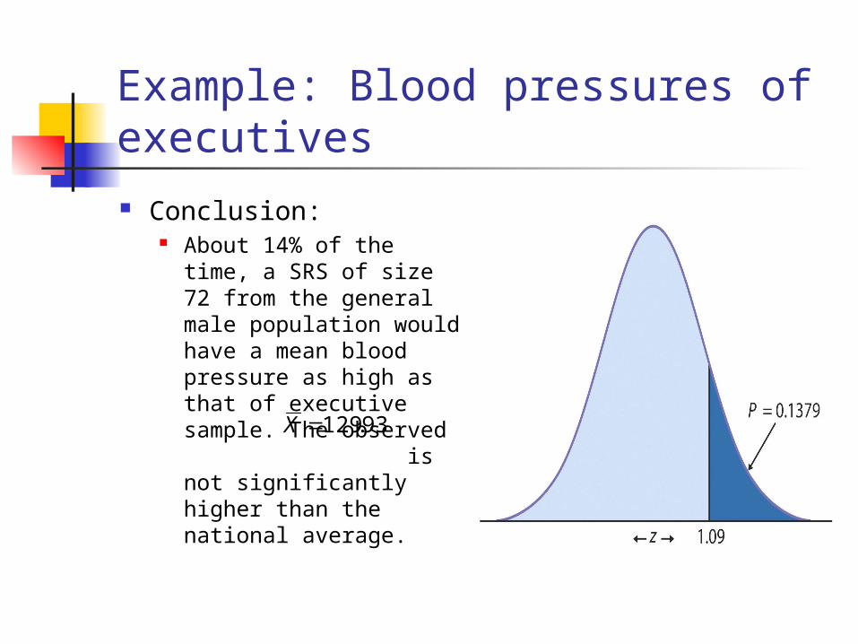
Example: Blood pressures of executives

Conclusion: About 14% of the time, a

SRS of size 72 from the general male population would have a mean blood pressure as high as that of executive sample. The observed is not significantly higher than the national average.

93.129X

Example: A company-wide health promotion campaign The company medical director institutes a health

promotion campaign to encourage employees to exercise more and eat a healthier diet. One measure of the effectiveness of such a program is a drop in blood pressure. Choose a random sample of 50 employees, and compare their blood pressures from annual physical examination given before the campaign and again a year later. The mean change in blood pressure for these n = 50 employees is . We take the population standard deviation to be = 20. Use = 5%.

6X

Example: A company-wide health promotion campaign Hypotheses:

H0: =0

Ha: < 0 Test statistic:

P-value:

12.25020

060

n

xz

0170.0)12.2( zPP

Example: A company-wide health promotion campaign Conclusion:

A mean change in blood pressure of –6 or better would occur only 17 times in 1000 samples if the campaign had no effect on the blood pressures of the employees. This is convincing evidence that the mean blood pressure in the population of all employees has decreased.

Example:Testing Pharmaceutical products The Deely Laboratory analyzes pharmaceutical products to

verify the concentration of active ingredients. Such chemical analyses are not perfectly precise. Repeated measurements on the same specimen will give slightly different results. The results of repeated measurements follow a Normal distribution quite closely, the analysis procedure has no bias, so that the mean of the population of all measurements is the true concentration in the specimen. The standard deviation of this distribution is a property of the analytical procedure and is known to be = 0.0068 gram per liter. The laboratory analyzes each specimen three times and reports the mean results.

Example:Testing Pharmaceutical products

A client sends a specimen for which the concentration of active ingredient is supposed to be 0.86%. Deely’s three analyses give concentrations

0.8403 0.8363 0.8447

Is there significant evidence at the 1% level that the true concentration is not 0.86%?

Example:Testing Pharmaceutical products

Hypotheses:H0: = 0.86

Ha: 0.86

Test Statistic: The mean of the three analyses is . The one sample z test statistic is therefore 99.4

30068.

86.8404.0

n

xz

8404.X

Example:Testing Pharmaceutical products

We do not need to find the exact P-value to assess significance at the = 0.01 level. Look in the table A under tail area 0.005 because the alternative is two-sided. The z-values that are significant at the 1% level are z > 2.575 and z < -2.575.

Our observed z = -4.99 is significant

P-value versus fixed In our example , we concluded that the test

statistic z = -4.99 is significant at the 1% level. The observed z is far beyond the critical value for

= 0.01, and the evidence against H0 is far stronger than 1% significance suggests.

The P-value P = .0000006 (from a statistical software) gives a better sense of how strong the evidence is.

The P-value is the smallest level at which the data are significant.

Inference for the Mean of a Population

Both confidence intervals and tests of significance for the mean of a Normal population are based on the sample mean , which estimates the unknown .

The sampling distribution of depends on .

There is no difficulty when is known. When is unknown, we must estimate it. The sample standard deviation s is used to

estimate the population standard deviation .

X

X

The t-distribution Suppose we have a simple random sample of size n

from a Normally distributed population with mean and standard deviation .

The standardized sample mean, or one-sample z statistic

has the standard Normal distribution N(0, 1). When we substitute the standard deviation of the mean

(standard error) s /n for the /n, the statistic does not have a Normal distribution.

n

xz

0

The t-distribution It has a distribution called t-distribution. The t-distribution

Suppose that a SRS of size n is drawn from a N(, ) population. Then the one sample t statistic

has the t-distribution with n-1 degrees of freedom. There is a different t distribution for each sample size. A particular t distribution is specified by giving the

degrees of freedom.

ns

xt

The t-distribution We use t(k) to stand for t

distribution with k degrees of freedom.

The density curves of the t-distributions are symmetric about 0 and are bell shaped.

The spread of t distribution is a bit greater than that of standard Normal distribution.

As degrees of freedom k increase, t(k) density curve approaches the N(0, 1) curve.

The one –Sample t Confidence Interval Suppose that an SRS of size n is drawn from a population

having unknown mean . A level C confidence interval for is

Where t* is the value for the t (n-1) density curve with area C between –t* and t*. The margin of error is

This interval is exact when the population distribution is Normal and is approximately correct for large n in other cases.

n

stx *

n

st *

Example: Estimating the level of Vitamin C

The following data are the amount of vitamin C, measured in milligram per 100 grams (mg/100g) of the corn soy blend (dry basis), for a random sample of size 8 from a production run: 26 31 23 22 11 22 14 31

We want to find a 95% confidence interval for , the mean vitamin C content of the corn soy blend (CSB) produced during this run.

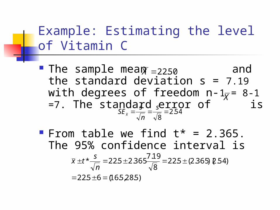
Example: Estimating the level of Vitamin C

The sample mean and the standard deviation s = 7.19 with degrees of freedom n-1 = 8-1 =7. The standard error of is

From table we find t* = 2.365. The 95% confidence interval is

50.22X

X

54.28

s

n

sSEx

)5.28,5.16(65.22

)54.2)(365.2(5.228

19.7365.25.22*

n

stx

The one-sample t test:Summary

Example: Is the Vitamin C level correct?

The specifications for the CSB state that the mixture should contain 2 pounds of vitamin premix fro every 2000 pounds of product. These specifications are designed to produce a mean () vitamin C content in the final product of 40mg/100 g. We test the null hypothesis that the mean vitamin C content of the production run in the previous example conforms to these specifications. Use = 5%.

Example: Is the Vitamin C level correct?

Hypotheses: H0: = 40

Ha: 40 Test statistic:

P-value:

Because the degrees of freedom are n-1 =7, this t statistic has t(7) distribution.

88.682.7

405.220

ns

xt

)88.6(2 tPP

Example: Is the Vitamin C level correct? From the largest entry in

the df =7 line of the table we see that

We conclude that the P-value is less than 20.0005, or P < .001.

We reject H0 and conclude that the vitamin C content for this run is below the specification.

0005.)408.5( tP

Matched Pairs t procedures Comparative studies are usually preferred to

single-sample investigations because of the protection they offer against confounding.

In a matched pairs study, subjects are matched in pairs and the outcomes are compared within each matched pair.

One situation calling for matched pairs is before-and-after observations on the same subjects.

Matched Pairs t procedures A matched pair analysis is needed when there are

two measurements or observations on each individual and we want to examine the change from the first to the second.

For each individual, subtract the “before” measure from the “after” measure.

Analyze the difference using the one-sample confidence interval and significance testing procedures.

Example: The effect of language instruction

A company contracts with a language institute to provide individualized instruction in foreign languages for its executives who will be posted overseas. Is the instruction effective? Last year 20 executives studied French. All had some knowledge of French, so they were given the Modern Language Association’s listening test of understanding of spoken French before the instruction began. After several weeks of immersion in French, the executives took the listening test again. The following table gives the pretest and posttest scores.

Example: The effect of language instruction

Example: The effect of language instruction

To analyze these data Subtract pretest score from the posttest score. These differences appear in the “gain” column in

previous table. These 20 differences form a single sample. To assess whether the institute significantly improved

the executives’ comprehension of spoken French we test

H0: = 0

Ha: > 0

Example: The effect of language instruction

Here is the mean improvement that would be achieved if the entire population of executives received similar instruction.

The null hypothesis says that no improvement occurs, and the alternative hypothesis says that posttest scores are higher on the average.

The 20 differences have 893.2 and 5.2 sX

Example: The effect of language instruction

The one sample t statistic is therefore

P-value is found from the t(19) distribution.

T-table shows that 3.86 lies between the upper .001 and .0005 critical values of the t(19) distribution. The P-value therefore lies between these values.

86.320893.2

05.20

ns

xt

)86.3( tPP

Example: The effect of language instruction

Conclusion: The improvement in scores was significant. We

have strong evidence that the posttest scores are systematically higher.

A statistically significant but very small improvement in language ability would not justify the expense of the individualized instruction. A confidence interval allows us to estimate the amount of improvement.

Example: The effect of language instruction

Find a 90% confidence interval for the mean improvement in the entire population. The critical value t* = 1.729 from t-table for

90% confidence. The confidence interval is:

)62.3,38.1(

12.15.220

893.2729.15.2*

n

stx