This content has been downloaded from IOPscience. Please scroll down to see the full text.

Download details:

IP Address: 128.178.27.45

This content was downloaded on 22/04/2014 at 08:34

Please note that terms and conditions apply.

Bulk velocity measurements by video analysis of dye tracer in a macro-rough channel

View the table of contents for this issue, or go to the journal homepage for more

2014 Meas. Sci. Technol. 25 035003

(http://iopscience.iop.org/0957-0233/25/3/035003)

Home Search Collections Journals About Contact us My IOPscience

Measurement Science and Technology

Meas. Sci. Technol. 25 (2014) 035003 (11pp) doi:10.1088/0957-0233/25/3/035003

Bulk velocity measurements by videoanalysis of dye tracer in a macro-roughchannel

T Ghilardi, M J Franca and A J Schleiss

Laboratory of Hydraulic Constructions (LCH), Ecole Polytechnique Federale de Lausanne (EPFL),Station 18, 1015 Lausanne, Switzerland

E-mail: tamara.ghilardi@epfl.ch

Received 26 June 2013, revised 1 November 2013Accepted for publication 2 January 2014Published 5 February 2014

AbstractSteep mountain rivers have hydraulic and morphodynamic characteristics that hinder velocitymeasurements. The high spatial variability of hydraulic parameters, such as water depth (WD),river width and flow velocity, makes the choice of a representative cross-section to measure thevelocity in detail challenging. Additionally, sediment transport and rapidly changing bedmorphology exclude the utilization of standard and often intrusive velocity measurementtechniques. The limited technical choices are further reduced in the presence ofmacro-roughness elements, such as large, relatively immobile boulders. Tracer trackingtechniques are among the few reliable methods that can be used under these conditions toevaluate the mean flow velocity. However, most tracer tracking techniques calculate bulk flowvelocities between two or more fixed cross-sections. In the presence of intense sedimenttransport resulting in an important temporal variability of the bed morphology, dead waterzones may appear in the few selected measurement sections. Thus a technique based on theanalysis of an entire channel reach is needed in this study. A dye tracer measurement techniquein which a single camcorder visualizes a long flume reach is described and developed. Thisallows us to overcome the problem of the presence of dead water zones. To validate this videoanalysis technique, velocity measurements were carried out on a laboratory flume simulating atorrent, with a relatively gentle slope of 1.97% and without sediment transport, using severalcommonly used velocity measurement instruments. In the absence of boulders, salt injections,WD and ultrasonic velocity profiler measurements were carried out, along with dye injectiontechnique. When boulders were present, dye tracer technique was validated only bycomparison with salt tracer. Several video analysis techniques used to infer velocities weredeveloped and compared, showing that dye tracking is a valid technique for bulk velocitymeasurements. RGB Euclidean distance was identified as being the best measure of theaverage flow velocity.

Keywords: bulk flow velocity, macro-rough channel, dye tracer tracking

(Some figures may appear in colour only in the online journal)

1. Introduction

Mountain rivers occupy a significant part of world catchments.Although they control sediment supply to lowland rivers,relatively few studies have been carried out on these torrents.They are characterized by longitudinal slopes ranging from

0.1% to 20% (Papanicolaou et al 2004) and by a widegrain size distribution composed of fine mobile sedimentsand large, relatively immobile, boulders (Rickenmann 2001,Yager et al 2007), which can be arranged randomly or in rows(Pagliara and Chiavaccini 2006). In torrents, the water depth(WD) is small in comparison to the roughness elements, and

0957-0233/14/035003+11$33.00 1 © 2014 IOP Publishing Ltd Printed in the UK

Meas. Sci. Technol. 25 (2014) 035003 T Ghilardi et al

the sediment transport can be intense. Bed morphology andhydraulic parameters, such as WD and flow velocity, have highspatial variability, and in the presence of sediment transport,high temporal variability can also be observed in the above-mentioned parameters (Recking et al 2009). Challenges inmeasuring hydraulic parameters under these conditions arefound not only in the field (Calkins and Dunne 1970, Churchand Kellerhals 1970) but also in laboratory experiments(Recking 2006, Pagliara 2007). High spatial variability of thechannel morphology does not allow sampling on a regulargrid, while the high temporal variability does not allow theinstallation of fixed systems. The presence of macro-roughnesselements hinders the use of methods sampling a large flowsurface, the small WD excludes most intrusive techniquessince these would disturb the flow, and the presence of intensesediment transport excludes the use of fragile instruments.Thus most of the existing velocity measurement techniquesare not appropriate, and selecting one or several representativecross-sections (i.e. average or typical cross-sections) toestimate average velocities is challenging in macro-roughmountain torrents (Calkins and Dunne 1970). Due to thespatiotemporal variability, hydraulic parameters such as theWD and the average flow velocity are often not measured butestimated indirectly using empirical relationships, for exampleresistance equations (Yager et al 2007, Recking et al 2009,Pagliara et al 2010, Heyman et al 2013).

The present paper focuses on bulk flow velocitymeasurement techniques in an experimental flume. Severaldifficulties in performing velocity measurements can beidentified for our sediment transport flume experiments(Ghilardi and Schleiss 2012): small average flow depth(between 0.027 and 0.053 m); high variability of WD both inspace and time (up to 0.1 m); mobile and rapidly changingbed; intense sediment transport; roughness elements oftenprotruding from the water (in our particular case, due to thepresence of boulders); small flume width (here, 0.25 m). Onetechnique, based on video analysis of dye tracer over an entireflume reach, proved to be adequate for estimating channel flowvelocities.

In section 2, a review of some existing velocitymeasurement techniques is presented, and their application tothe hydraulic conditions of steep rough channels is described.In section 3, the experimental facility is described. Section 4presents the procedure of the dye tracking technique leadingto the estimation of the bulk flow velocities. Section 5compares the dye tracer technique and data treatment to othervelocity measurement methods for validation purposes. Saltand dye tracer tracking measurements are the only availablemethods that are applicable in the presence of boulders. Inthe absence of boulders, direct ultrasonic velocity profiles,velocity measurements and mean velocities inferred from WDmeasurements are also used for comparison. In section 6 themain conclusions are given.

2. Review of main velocity measurementtechniques

Most velocity estimation techniques yield local informationabout the flow conditions. These methods require that one

or more representative cross-sections are identified. The dataobtained for the cross-sections are then averaged to estimatethe average bulk flow velocity. Techniques that are commonlyused to measure velocity in open-channel flows include: waterdepth (WD) measurements; micro-propeller vertical profiling;acoustic Doppler velocimeter (ADV); ultrasonic velocityprofiles (UVP); acoustic Doppler velocity profiles (ADVP);acoustic Doppler current profilers (ADCP); hot wire; laserDoppler anemometry (LDA); electromagnetic current meters(EMC); Pitot probes; particle image velocimetry (PIV) andparticle tracking velocimetry (PTV); tracer tracking methods,with various types of tracers (salt and dyes).

WD measurements (using point-gauges, ultrasonicdistance meters and other instruments) and back-calculation offlow velocity seems to be a simple technique for determiningaverage flow velocities when the discharge is known. However,as mentioned before, representative cross-sections are difficultto identify and other challenges need to be tackled. It is difficultto determine the base level (bed level) from which the WDhas to be measured, primarily because of the high relativeroughness encountered in mountain rivers. The uncertainty ofthe WD measurement is directly linked to the ratio betweenthe WD and the roughness height (Rickenmann 1990, Recking2006). Thus large errors may occur in WD measurementsin torrents, since the elevation of the bed changes abruptlyover short distances. The bed level is even more difficult todetermine in the presence of intense bedload, because of theexistence of a moving layer and rapid changes in the bedconfiguration. Moreover, the water surface is highly irregular,thus making its unambiguous measurement difficult.

Micro-propeller vertical profiling (full- and partial-depth(Church and Kellerhals 1970)) are easy and precise ways tomeasure the mean velocities of flows with simple geometriesin clear-water prismatic open-channels. In the flows targetedin the present research, however, several disadvantages of thismethod exist, including the sensitivity of the instrumentationblades to impact with sediments transported by the flow andthe intrusiveness of the method, which causes local erosionwhen measuring velocities near a mobile bed.

Techniques based on the Doppler shift frequency ofthe echoes reflected by small suspended particles (seeding)comprise: ADV, UVP, 3D ADVP and ADCP.

ADV, composed of one central emitter and three (orfour) sound receivers, allows point measurements of the threecomponents of the flow velocity. It has been widely used fora long time in laboratory (Kraus et al 1994) and field (Wilcoxand Wohl 2007) studies of open-channel flows. ADVs needto be immersed in the water, thus are intrusive, and requirespace to accommodate the probes and the near field neededbetween the emitter and the measuring point. In shallow flowswith restricted space for the measurements, this technique islimited. Furthermore, when the aim is to obtain bulk-averagevelocities, ADV requires a large amount of measuring points.

UVP (Amini et al 2009) measure instantaneous velocity1D profiles along a beam axis. Several beams can be used toobtain velocity profiles at a single cross-section and an averagecross-section velocity can then be calculated. Bathymetryuncertainties for UVP measurements are normally of the size

2

Meas. Sci. Technol. 25 (2014) 035003 T Ghilardi et al

of one measuring gate. Thus this is not relevant in the presentcase for the calculation of vertical averaged velocities. UVPtransducers need to be partially immersed in the water; thusUVP measurement is an intrusive technique. In the presentcase, with widely varying water levels and bed morphology, theuse of UVP with a regular sampling grid for the cross-sectionsis not possible. Moreover, the size of mobile sediments is notnegligible with respect to the WD, and the signal echoed bygravel interferes with the backscattered signal.

ADVP, developed at the Ecole Polytechnique Federale deLausanne (EPFL) (Franca and Lemmin 2006), allow full-depthquasi-instantaneous 3D velocity profiling and are suitablefor use both in the field (Franca et al 2008) and in thelaboratory (Blanckaert and De Vriend 2004, Leite Ribeiro et al2012, Dugue et al 2013). ADVP are intrusive, and while thisinfluence is negligible for slow flow, at high flow velocitiessuch as those considered in this study, ADVP change the flowcharacteristics and influence flow velocities. The presence ofmacro-rough elements and gravel bars precludes the use ofADVP because they require considerable free space.

ADCP, constituted typically of a central body wherediverging transducers working simultaneously as emitters andreceptors are installed, are commonly used for large-scalestudies. They are used for estimating large features of flows inlakes (Lorke and Wuest 2005) and rivers (Le Coz et al 2008).The dimensions of ADCP instrumentation and the weight donot allow easy and fine displacement of the instrumentationin shallow flows with such singularities and obstacles as bedforms and large boulders.

Techniques commonly used to measure flow velocitiesin fluid mechanics, such as hot wire anemometry (cf Hinze(1975) for details) and LDA (cf Nezu and Nakagawa(1993) for details), are not adequate in the case of intensebedload transport and spatial variability of the channel bed.Furthermore, the apparatus is not easily movable, which isimportant when local conditions change so abruptly in spacesuch as the herein treated channel flows. With the presence ofboulders and bed forms, the installation of such equipment ina flume is not easy. Regarding LDA, hidden (shadow) areas ofthe flow hinder the penetration of the laser light.

Electromagnetic current meters use the Faraday principleof electromagnetic induction, stating that the voltage producedby water moving in a magnetic field is proportional to thevelocity of the water (MacVicar et al 2007). ECM is used inlaboratory and field research (Roy et al 2004), for 2D velocitymeasurements. This instrumentation is robust, but too intrusiveand thus disturbing to the flow (Voulgaris and Trowbridge1998).

Pitot probes (USBR 1980), commonly used for fieldmeasurements, are also too intrusive. Furthermore, the riskof damage is high when used in shallow flow with intensesediment transport.

PIV and PTV, particularly large-scale particle imagevelocimetry (LSPIV), are techniques for measuring velocityfields based on image analysis, i.e. tracking light particlestransported by the flow. PIV uses a laser to illuminate particletransport by a thin layer in the flow (Raffel et al 1998, Pokrajacet al 2007), while LSPIV uses only light particles transported

on the water surface (Fujita et al 1998, van Prooijen andUijttewaal 2002, Jodeau et al 2008, Muste et al 2008, Kantoushet al 2011, Mattioli et al 2012). The light particles on thesurface are representative of the surface flow velocity andrecirculation cells with signatures at the free surface (vanProoijen and Uijttewaal 2002) and can be applied in shallowwater, where the horizontal velocity is predominant andgreatly exceeds the vertical velocity. These applications needextremely controlled light conditions and special equipment,and in the presence of intense sediment transport, they presentproblems in the identification of tracking particles.

If the reach average bulk velocity has to be known, as wasthe case in our research project, tracer tracking techniquesare sufficient (Ghilardi and Schleiss 2011, 2012). Thesetechniques are applicable in both the field (Calkins and Dunne1970, Church and Kellerhals 1970) and the laboratory (Cao1985, Rickenmann 1990, Weichert 2005, Recking et al 2008).Four types of tracer exist: salt, dye, other traceable chemicalcompounds and radioisotopes (Church and Kellerhals 1970).The first two tracer types are the most widely used. The tracertravel time can be calculated either between the injectionpoint and the measurement point (Calkins and Dunne 1970) orbetween two or more sampling positions (Rickenmann 1990,Recking et al 2008). The latter method is generally used forlaboratory experiments.

In salt tracer velocity measurement, a slug of salt solutionis injected into the water, and the water conductivity increasesdue to the passage of the salt cloud. This change in conductivitycan be recorded at one or more measurement cross-sectionsby means of electrode couples, providing conductivity–timecurves. These electrode couples are often formed by twovertical metal strips attached to opposite walls of the channelat a selected cross-section (Smart and Jaggi 1983, Weichert2005). In the case of high temporal bed variability (verticalfluctuations), the electrodes need to be long enough toaccommodate the changes in the bed level. The fluid velocitycan be calculated as the distance between two cross-sectionsdivided by the travel time of the tracer cloud between them.The starting point of conductivity increase is generally clearlydefined. The identification of the end point is often difficultbecause the tail of the curve can be relatively long (Day 1976,Rickenmann 1990). This is also the case when working withdye as a tracer. Water conductivity can also be measuredby conductivity-meter probes, which measure the changein conductivity between two electrodes placed only a fewmillimetres apart from each other. Since intrusive and local,the choice of a representative point for the measurement isneeded. In our study, we used vertical metal strips attachedto the flume walls to carry out conductivity measurements, inorder to obtain average values over the cross-section.

Video camera-based techniques are often used inhydraulics research to estimate flow velocities (Le Coz et al2010, Mattioli et al 2012) and concentration fields (Thomasand Marino 2012, Nogueira et al 2013). Dye tracer velocitiescan be estimated by means of video analysis. Recking et al(2008) described the introduction of a slug of colorant in aflume and the analysis of the passage of the cloud betweentwo positions in the flume using two video cameras (recording

3

Meas. Sci. Technol. 25 (2014) 035003 T Ghilardi et al

at 20 frames per second) placed 4 m apart from each other atthe flume surface. Only two cross-sections were thus analysed.The two camcorders must be perfectly synchronized for thetravel time to be calculated correctly. Recking (2006) reportedthat for highly turbulent flow (Re > 6000), no infiltrationof the colorant in the bed was observed; thus, no delay in thetracer release was introduced. He emphasized that for steepslopes (9%) and small relative WDs, the signal can be quitenoisy due to the rapid changes in light conditions inducedby the fluctuating water surface. Nevertheless, the shape of theconcentration curve remains the same. The video was analysedin grey scale, and the colorant plume was identified by a peakin grey scales (the image becomes darker). The peak velocitywas used by Recking to estimate the bulk velocity.

Tracer tracking measurements over time at one fixedposition provide three types of information: the initial risein concentration, the peak concentration and the centre ofmass of the tracer cloud. According to Calkins and Dunne(1970), the initial rise in concentration is a measure of themaximum velocity through the channel reach. The peak inconcentration is commonly used to obtain the travel timeand sometimes to estimate the bulk flow velocity. Calkinsand Dunne (1970) and Church and Kellerhals (1970) claimthat the time delay of the centroid of the concentration curvebetween two points represents the mean residence time ofthe tracer in the reach between the aforementioned pointsand thus can be used to estimate the mean velocity in thereach. Researchers primarily use centroid velocities to estimatebulk flow velocities (Church and Kellerhals 1970, Daviesand Jaggi 1981, Smart and Jaggi 1983, Rickenmann 1990,Weichert 2005), although some researchers use the peak tracerconcentration (Cao 1985, Recking 2006, Recking et al 2008).Cao (1985) compared the velocities estimated using the peakand the centre of mass of the salt solution and those estimatedfrom WD measurement and found that velocities estimatedusing the peak of the conductivity travel time were closerto those estimated from WD measurement. He attributes thisoutcome to the presence of ‘dead zones’, characterized bysmall longitudinal velocities, that result in slow release of thetracer after the passage of the main flow and the formation oflong tails in the conductivity curves (Cao 1985). Accordingto Day (1976) and Church and Kellerhals (1970), gross errorsin salt tracking can occur if the electrode is placed in a zonewith no longitudinal velocity component (a dead zone) in thestream.

The main difficulty with the salt and dye tracertechniques is the choice of representative cross-sections for themeasurements, as discussed in the introduction. For instance,if the measurement is carried out in a section where a dead zoneis present, the final result could be strongly affected. A newmethod for analysing a whole reach at once is thus presentedin this study.

Table 1 summarizes a critical assessment stating the mainadvantages and drawbacks of the aforementioned techniquesfor conditions where channel bed morphology is quiteheterogeneous, the roughness elements have low submergenceand intense bedload occurs. The intrusiveness criterion isrelevant for small flow depth. Intrusive methods would greatly

influence the flow conditions and the bed morphology. Thesediment transport criterion addresses both the bedload andthe suspended load. It indicates if the presence of sedimenttransport would be a problem for the integrity of the techniqueand for the field of view of this (i.e. LDA). The numberof measures criterion refers to the sampling grid densitynecessary to obtain bulk-average velocities, which may betime consuming and difficult to position in shallow flows.The spatiotemporal variability, including the presence ofprotruding boulders, is a problem for all the techniquesrequiring a regular sampling grid. The presence of dead waterzones complicates the choice of a representative cross-section.This is especially the case for tracer tracking between twofixed sections, since the position of dead water zones variesin space and time in a way that measurement positions areinfluenced. Finally, the presence of air in the flow, which maybe relevant immediately downstream of boulders, would be amain drawback for some of the measurement techniques.

3. Experimental details

The velocity measurement technique presented herein wasdeveloped within the framework of a research project focusedon analysing the impact that randomly distributed relativelyimmobile boulders have on sediment transport in steep-slope rivers. This research was carried out using mobile bedlaboratory experiments conducted using a tilting flume 8 mlong (with a usable length of 7 m) and 0.25 m wide (figure 1)at the Laboratory of Hydraulic Constructions (LCH) of theEcole Polytechnique Federale de Lausanne (EPFL) (Ghilardiand Schleiss 2011, 2012).

For the comparison with the standard velocitymeasurement techniques, the flume slope was set to α =1.97% to produce a high WD but no sediment transport. Waterdischarge, fed constantly by a closed pumping system, wasmeasured using an electromagnetic flow meter ( ± 0.01 l s−1).A plane bed was prepared with sediments with the followinggrain size distribution characteristics: dm = d65 = 11.9 mm,d30 = 7.1 mm, and d90 = 19 mm, where dm is the mean grainsize, corresponding to d65, and dx is the grain size diameterat which x% by weight of the sediments are smaller. Duringthe experiments, no sediment transport occurred; thus, no bedforms were observed.

In the case of a plane bed test without boulders, flowvelocities were measured by four techniques for three differentdischarge rates: 5.0, 7.25 and 9.5 l s−1. This range was chosento yield a sufficiently high WD for UVP measurement (37 mmon average for Q = 5.0 l s−1) on the one hand and avoidlocal scouring downstream of boulders and sediment transport(limiting the discharge to Q = 9.5 l s−1) on the other hand. UVPand WD measurements yielded estimates of the flow velocityfor a given cross-section. For both methods, 17 cross-sections,spaced 0.1 m apart longitudinally, were gauged at distancesbetween 2.55 and 4.25 m from the flume inlet (see figure 1).The water and bed levels were measured at 12 equally spacedlocations—thus, every 0.02 m—across every section using apoint-gauge. Three 4 MHz UVP probes were placed in thecross-section, at the middle, first quarter and third quarter of

4

Meas. Sci. Technol. 25 (2014) 035003 T Ghilardi et al

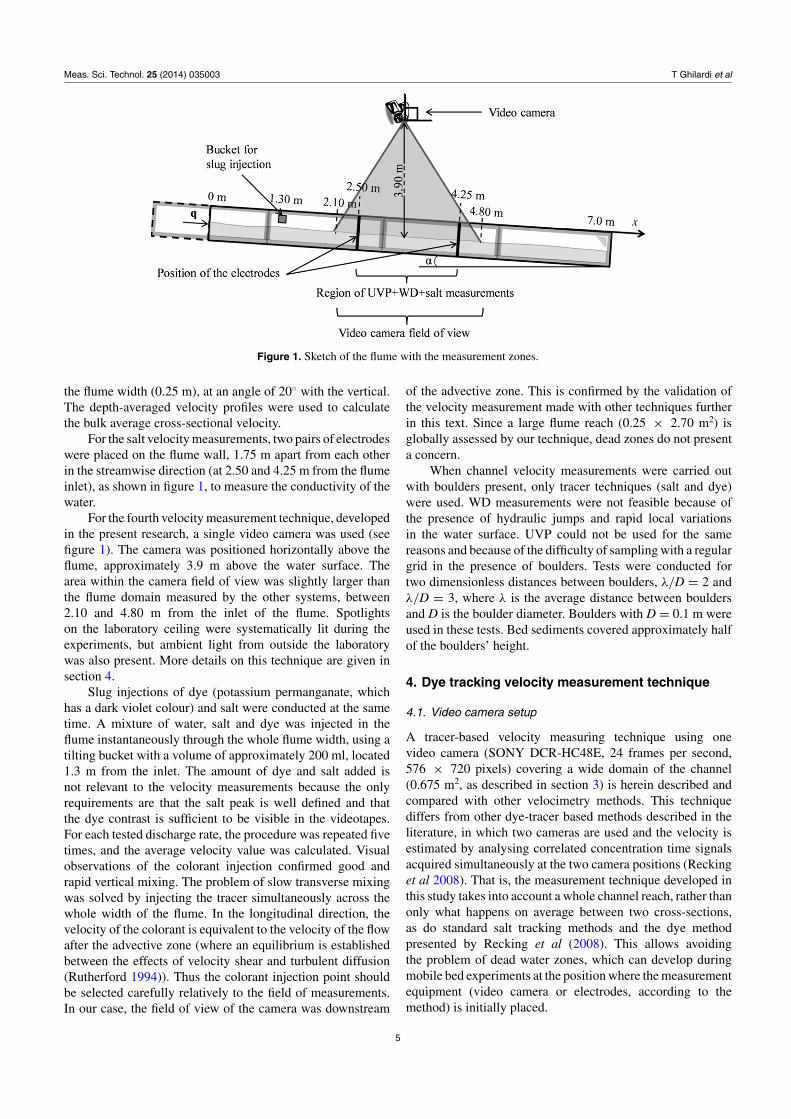
Figure 1. Sketch of the flume with the measurement zones.

the flume width (0.25 m), at an angle of 20◦ with the vertical.The depth-averaged velocity profiles were used to calculatethe bulk average cross-sectional velocity.

For the salt velocity measurements, two pairs of electrodeswere placed on the flume wall, 1.75 m apart from each otherin the streamwise direction (at 2.50 and 4.25 m from the flumeinlet), as shown in figure 1, to measure the conductivity of thewater.

For the fourth velocity measurement technique, developedin the present research, a single video camera was used (seefigure 1). The camera was positioned horizontally above theflume, approximately 3.9 m above the water surface. Thearea within the camera field of view was slightly larger thanthe flume domain measured by the other systems, between2.10 and 4.80 m from the inlet of the flume. Spotlightson the laboratory ceiling were systematically lit during theexperiments, but ambient light from outside the laboratorywas also present. More details on this technique are given insection 4.

Slug injections of dye (potassium permanganate, whichhas a dark violet colour) and salt were conducted at the sametime. A mixture of water, salt and dye was injected in theflume instantaneously through the whole flume width, using atilting bucket with a volume of approximately 200 ml, located1.3 m from the inlet. The amount of dye and salt added isnot relevant to the velocity measurements because the onlyrequirements are that the salt peak is well defined and thatthe dye contrast is sufficient to be visible in the videotapes.For each tested discharge rate, the procedure was repeated fivetimes, and the average velocity value was calculated. Visualobservations of the colorant injection confirmed good andrapid vertical mixing. The problem of slow transverse mixingwas solved by injecting the tracer simultaneously across thewhole width of the flume. In the longitudinal direction, thevelocity of the colorant is equivalent to the velocity of the flowafter the advective zone (where an equilibrium is establishedbetween the effects of velocity shear and turbulent diffusion(Rutherford 1994)). Thus the colorant injection point shouldbe selected carefully relatively to the field of measurements.In our case, the field of view of the camera was downstream

of the advective zone. This is confirmed by the validation ofthe velocity measurement made with other techniques furtherin this text. Since a large flume reach (0.25 × 2.70 m2) isglobally assessed by our technique, dead zones do not presenta concern.

When channel velocity measurements were carried outwith boulders present, only tracer techniques (salt and dye)were used. WD measurements were not feasible because ofthe presence of hydraulic jumps and rapid local variationsin the water surface. UVP could not be used for the samereasons and because of the difficulty of sampling with a regulargrid in the presence of boulders. Tests were conducted fortwo dimensionless distances between boulders, λ/D = 2 andλ/D = 3, where λ is the average distance between bouldersand D is the boulder diameter. Boulders with D = 0.1 m wereused in these tests. Bed sediments covered approximately halfof the boulders’ height.

4. Dye tracking velocity measurement technique

4.1. Video camera setup

A tracer-based velocity measuring technique using onevideo camera (SONY DCR-HC48E, 24 frames per second,576 × 720 pixels) covering a wide domain of the channel(0.675 m2, as described in section 3) is herein described andcompared with other velocimetry methods. This techniquediffers from other dye-tracer based methods described in theliterature, in which two cameras are used and the velocity isestimated by analysing correlated concentration time signalsacquired simultaneously at the two camera positions (Reckinget al 2008). That is, the measurement technique developed inthis study takes into account a whole channel reach, rather thanonly what happens on average between two cross-sections,as do standard salt tracking methods and the dye methodpresented by Recking et al (2008). This allows avoidingthe problem of dead water zones, which can develop duringmobile bed experiments at the position where the measurementequipment (video camera or electrodes, according to themethod) is initially placed.

5

Meas. Sci. Technol. 25 (2014) 035003 T Ghilardi et al

(a)

(b)

(c)

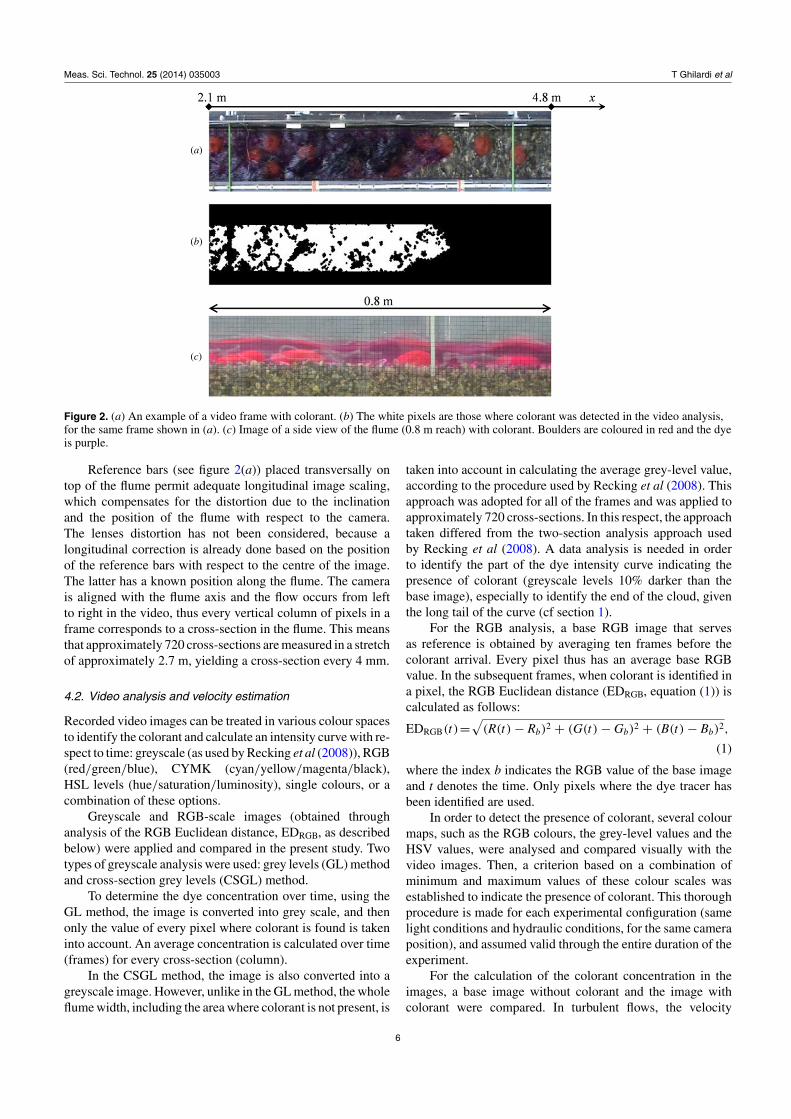
Figure 2. (a) An example of a video frame with colorant. (b) The white pixels are those where colorant was detected in the video analysis,for the same frame shown in (a). (c) Image of a side view of the flume (0.8 m reach) with colorant. Boulders are coloured in red and the dyeis purple.

Reference bars (see figure 2(a)) placed transversally ontop of the flume permit adequate longitudinal image scaling,which compensates for the distortion due to the inclinationand the position of the flume with respect to the camera.The lenses distortion has not been considered, because alongitudinal correction is already done based on the positionof the reference bars with respect to the centre of the image.The latter has a known position along the flume. The camerais aligned with the flume axis and the flow occurs from leftto right in the video, thus every vertical column of pixels in aframe corresponds to a cross-section in the flume. This meansthat approximately 720 cross-sections are measured in a stretchof approximately 2.7 m, yielding a cross-section every 4 mm.

4.2. Video analysis and velocity estimation

Recorded video images can be treated in various colour spacesto identify the colorant and calculate an intensity curve with re-spect to time: greyscale (as used by Recking et al (2008)), RGB(red/green/blue), CYMK (cyan/yellow/magenta/black),HSL levels (hue/saturation/luminosity), single colours, or acombination of these options.

Greyscale and RGB-scale images (obtained throughanalysis of the RGB Euclidean distance, EDRGB, as describedbelow) were applied and compared in the present study. Twotypes of greyscale analysis were used: grey levels (GL) methodand cross-section grey levels (CSGL) method.

To determine the dye concentration over time, using theGL method, the image is converted into grey scale, and thenonly the value of every pixel where colorant is found is takeninto account. An average concentration is calculated over time(frames) for every cross-section (column).

In the CSGL method, the image is also converted into agreyscale image. However, unlike in the GL method, the wholeflume width, including the area where colorant is not present, is

taken into account in calculating the average grey-level value,according to the procedure used by Recking et al (2008). Thisapproach was adopted for all of the frames and was applied toapproximately 720 cross-sections. In this respect, the approachtaken differed from the two-section analysis approach usedby Recking et al (2008). A data analysis is needed in orderto identify the part of the dye intensity curve indicating thepresence of colorant (greyscale levels 10% darker than thebase image), especially to identify the end of the cloud, giventhe long tail of the curve (cf section 1).

For the RGB analysis, a base RGB image that servesas reference is obtained by averaging ten frames before thecolorant arrival. Every pixel thus has an average base RGBvalue. In the subsequent frames, when colorant is identified ina pixel, the RGB Euclidean distance (EDRGB, equation (1)) iscalculated as follows:

EDRGB(t)=√

(R(t) − Rb)2 + (G(t) − Gb)2 + (B(t) − Bb)2,

(1)

where the index b indicates the RGB value of the base imageand t denotes the time. Only pixels where the dye tracer hasbeen identified are used.

In order to detect the presence of colorant, several colourmaps, such as the RGB colours, the grey-level values and theHSV values, were analysed and compared visually with thevideo images. Then, a criterion based on a combination ofminimum and maximum values of these colour scales wasestablished to indicate the presence of colorant. This thoroughprocedure is made for each experimental configuration (samelight conditions and hydraulic conditions, for the same cameraposition), and assumed valid through the entire duration of theexperiment.

For the calculation of the colorant concentration in theimages, a base image without colorant and the image withcolorant were compared. In turbulent flows, the velocity

6

Meas. Sci. Technol. 25 (2014) 035003 T Ghilardi et al

0.0 1.5 3.0 4.5 6.0 7.5 9.0 10.5 12.0 13.5 15.00

20

40

60

80

100

Time (s)

ED

RG

B (-

)

2.84 m3.59 m4.34 m

0.0 1.5 3.0 4.5 6.0 7.5 9.0 10.5 12.0 13.5 15.02

3

4

5

Pos

ition

(m

)

Time of CDM (s)

Tpeak1

Tpeak2

Tpeak3

TCDM1

TCDM2

TCDM3

velocity estimates( )( )

dx m

dt s

(a)

(b)

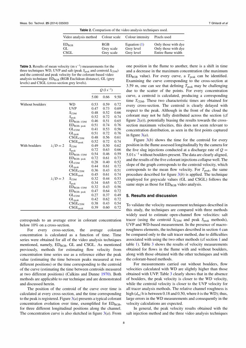
Figure 3. (a) An example of RGB Euclidean distance (EDRGB) time evolution for cross-sections at 2.84, 3.59 and 4.34 m (for colorantinjection without boulders at a discharge rate of 5.0 l s−1). The times of centroids (TCDM) and of peaks (Tpeak) are identified on the graph. Asketch of the concentration curve is given for each cross-section. (b) Position of the centroid CDM over time, estimated for each longitudinalposition for the five colorant injections.

Table 1. Comparison of the advantages (√

) and drawbacks (x) of the mentioned techniques to estimate bulk flow velocity in open-channelflows. In section 5 WD, UVP and salt (metal strips) are compared with the technique herein developed: dye (1 reach).

Method Advantages (√

)/Drawbacks (x)

Sediment Number of Spatiotemporal Dead waterIntrusiveness transport measures variability zones Aeration

Water depth √ x √ x √ √Micro-propeller x x x x x xADV x x x x x xUVP x x x x x xADVP x x x x √ xADCP x x x x x xHot wire x x x x √ xLDA √ x x x √ xECM x x x x x xPitot probe x x x x x xPIV/LSPIV √ √ √ √ x √Salt (probe) x √ x x x √Salt (metal strips) √ √ √ √ x √Dye (2 sections) √ √ √ √ x √Dye (1 reach) √ √ √ √ √ √

distribution is almost uniform within the flow depth, thusdetection of the dye intensity may be considered representativeof the total colorant concentration in the vertical layer and notonly of the flow surface.

Table 2 summarizes the characteristics and the differencesbetween the aforementioned video analysis methods.

Figure 2(a) shows a frame with colorant in the presenceof boulders, and figure 2(c) illustrates the coloured flow witha side view of the flume. Figure 2(b) shows in white the pixelswhere colorant has been detected during the video analysis.In some regions, the colorant could not be identified becauseof the reflection of light on the water surface. However, this

7

Meas. Sci. Technol. 25 (2014) 035003 T Ghilardi et al

Table 2. Comparison of the video analysis techniques used.

Video analysis method Colour scale Colour intensity Pixels used

EDRGB RGB Equation (1) Only those with dyeGL Grey scale Grey level Only those with dyeCSGL Grey scale Grey level Entire flume width

Table 3. Results of mean velocity (m s−1) measurements for thethree techniques WD, UVP and salt (peak Speak and centroid SCDM)and the centroid and peak velocity for the colorant-based videoanalysis technique: EDRGB (RGB Euclidean distance), GL (greylevels) and CSGL (cross-section grey levels).

Q (l s−1)

5.00 0.66 9.50

Without boulders WD 0.53 0.59 0.72UVP 0.47 0.73 0.69SCDM 0.48 0.52 0.66Speak 0.52 0.72 0.74EDRGB, CDM 0.46 0.51 0.65EDRGB, peak 0.51 0.74 0.76GLCDM 0.41 0.53 0.56GLpeak 0.51 0.72 0.76CSGLCDM 0.48 0.56 0.61CSGLpeak 0.52 0.72 0.74

With boulders λ/D = 2 SCDM 0.49 0.50 0.62Speak 0.72 0.63 0.66EDRGB, CDM 0.54 0.46 0.59EDRGB, peak 0.72 0.61 0.73GLCDM 0.28 0.40 0.52GLpeak 0.44 0.61 0.72CSGLCDM 0.36 0.43 0.51CSGLpeak 0.45 0.61 0.74

λ/D = 3 SCDM 0.32 0.44 0.53Speak 0.34 0.65 0.72EDRGB, CDM 0.32 0.43 0.56EDRGB, peak 0.47 0.64 0.72GLCDM 0.27 0.37 0.49GLpeak 0.42 0.62 0.72CSGLCDM 0.38 0.43 0.54CSGLpeak 0.39 0.60 0.72

corresponds to an average error in colorant concentrationbelow 10% on a cross-section.

For every cross-section, the average colorantconcentration is calculated as a function of time. Timeseries were obtained for all of the video analysis techniquesmentioned, namely, EDRGB, GL and CSGL. As mentionedpreviously, methods for estimating flow velocity fromconcentration time series use as a reference either the peakvalue (estimating the time between peaks measured at twodifferent positions) or the time corresponding to the centroidof the curve (estimating the time between centroids measuredat two different positions) (Calkins and Dunne 1970). Bothmethods are applicable to our technique and are demonstratedand discussed herein.

The position of the centroid of the curve over time iscalculated at every cross-section, and the time correspondingto the peak is registered. Figure 3(a) presents a typical colorantconcentration evolution over time, exemplified for EDRGB,for three different longitudinal positions along the channel.The concentration curve is also sketched in figure 3(a). From

one position in the flume to another, there is a shift in timeand a decrease in the maximum concentration (the maximumEDRGB value). For every curve, a Tpeak can be identified.Examining the curve corresponding to the cross-section at3.59 m, one can see that defining Tpeak may be challengingdue to the scatter of the points. For every concentrationcurve, a centroid is calculated, producing a correspondingtime TCDM. These two characteristic times are obtained forevery cross-section. The centroid is clearly delayed withrespect to the peak. Although in the front of the cloud thecolorant may not be fully distributed across the section (cffigure 2(a)), potentially biasing the results towards the cross-section maximum velocities, this does not seem relevant toconcentration distribution, as seen in the first points capturedin figure 3(a).

Figure 3(b) shows the time for the centroid for everyposition in the flume assessed longitudinally by the camera forthe five slug injections conducted at a discharge rate of Q =5.0 l s−1 without boulders present. The data are clearly aligned,and the results of the five colorant injections collapse well. Theslope of the graph corresponds to the centroid velocity, whichcorresponds to the mean flow velocity. For Tpeak, the sameprocedure described for figure 3(b) is applied. The techniqueemployed for greyscale values (GL and CSGL) follows thesame steps as those for EDRGB video analysis.

5. Results and discussion

To validate the velocity measurement techniques described inthis study, the techniques are compared with three methodswidely used to estimate open-channel flow velocities: salttracer (using the centroid SCDM and peak Speak methods),UVP and WD-based measurement. In the presence of macro-roughness elements, the techniques described in section 4 canbe compared only to the salt tracer method, due to difficultiesassociated with using the two other methods (cf section 1 andtable 1). Table 3 shows the results of velocity measurementsobtained for flows in the flume with and without boulders,along with those obtained with the other techniques and withthe colorant-based methods.

For measurements carried out without boulders, flowvelocities calculated with WD are slightly higher than thoseobtained with UVP. Table 3 clearly shows that in the absenceof boulders, the peak velocity is closer to the WD velocity,while the centroid velocity is closer to the UVP velocity forall tracer analysis methods. The relative channel roughness ishigh (dm/h is between 0.18 and 0.50, where h is the WD); thus,large errors in the WD measurements and consequently in thevelocity calculations are expected.

In general, the peak velocity results obtained with thesalt injection method and the three video analysis techniques

8

Meas. Sci. Technol. 25 (2014) 035003 T Ghilardi et al

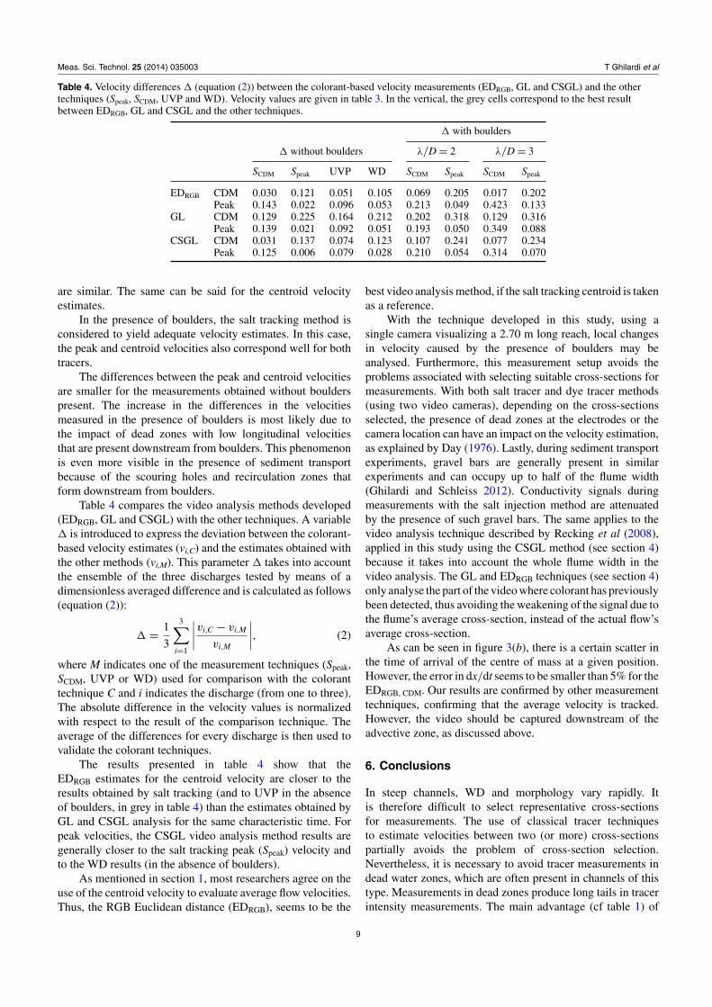
Table 4. Velocity differences � (equation (2)) between the colorant-based velocity measurements (EDRGB, GL and CSGL) and the othertechniques (Speak, SCDM, UVP and WD). Velocity values are given in table 3. In the vertical, the grey cells correspond to the best resultbetween EDRGB, GL and CSGL and the other techniques.

� with boulders

� without boulders λ/D = 2 λ/D = 3

SCDM Speak UVP WD SCDM Speak SCDM Speak

EDRGB CDM 0.030 0.121 0.051 0.105 0.069 0.205 0.017 0.202Peak 0.143 0.022 0.096 0.053 0.213 0.049 0.423 0.133

GL CDM 0.129 0.225 0.164 0.212 0.202 0.318 0.129 0.316Peak 0.139 0.021 0.092 0.051 0.193 0.050 0.349 0.088

CSGL CDM 0.031 0.137 0.074 0.123 0.107 0.241 0.077 0.234Peak 0.125 0.006 0.079 0.028 0.210 0.054 0.314 0.070

are similar. The same can be said for the centroid velocityestimates.

In the presence of boulders, the salt tracking method isconsidered to yield adequate velocity estimates. In this case,the peak and centroid velocities also correspond well for bothtracers.

The differences between the peak and centroid velocitiesare smaller for the measurements obtained without boulderspresent. The increase in the differences in the velocitiesmeasured in the presence of boulders is most likely due tothe impact of dead zones with low longitudinal velocitiesthat are present downstream from boulders. This phenomenonis even more visible in the presence of sediment transportbecause of the scouring holes and recirculation zones thatform downstream from boulders.

Table 4 compares the video analysis methods developed(EDRGB, GL and CSGL) with the other techniques. A variable� is introduced to express the deviation between the colorant-based velocity estimates (vi,C) and the estimates obtained withthe other methods (vi,M). This parameter � takes into accountthe ensemble of the three discharges tested by means of adimensionless averaged difference and is calculated as follows(equation (2)):

� = 1

3

3∑

i=1

∣∣∣∣vi,C − vi,M

vi,M

∣∣∣∣, (2)

where M indicates one of the measurement techniques (Speak,SCDM, UVP or WD) used for comparison with the coloranttechnique C and i indicates the discharge (from one to three).The absolute difference in the velocity values is normalizedwith respect to the result of the comparison technique. Theaverage of the differences for every discharge is then used tovalidate the colorant techniques.

The results presented in table 4 show that theEDRGB estimates for the centroid velocity are closer to theresults obtained by salt tracking (and to UVP in the absenceof boulders, in grey in table 4) than the estimates obtained byGL and CSGL analysis for the same characteristic time. Forpeak velocities, the CSGL video analysis method results aregenerally closer to the salt tracking peak (Speak) velocity andto the WD results (in the absence of boulders).

As mentioned in section 1, most researchers agree on theuse of the centroid velocity to evaluate average flow velocities.Thus, the RGB Euclidean distance (EDRGB), seems to be the

best video analysis method, if the salt tracking centroid is takenas a reference.

With the technique developed in this study, using asingle camera visualizing a 2.70 m long reach, local changesin velocity caused by the presence of boulders may beanalysed. Furthermore, this measurement setup avoids theproblems associated with selecting suitable cross-sections formeasurements. With both salt tracer and dye tracer methods(using two video cameras), depending on the cross-sectionsselected, the presence of dead zones at the electrodes or thecamera location can have an impact on the velocity estimation,as explained by Day (1976). Lastly, during sediment transportexperiments, gravel bars are generally present in similarexperiments and can occupy up to half of the flume width(Ghilardi and Schleiss 2012). Conductivity signals duringmeasurements with the salt injection method are attenuatedby the presence of such gravel bars. The same applies to thevideo analysis technique described by Recking et al (2008),applied in this study using the CSGL method (see section 4)because it takes into account the whole flume width in thevideo analysis. The GL and EDRGB techniques (see section 4)only analyse the part of the video where colorant has previouslybeen detected, thus avoiding the weakening of the signal due tothe flume’s average cross-section, instead of the actual flow’saverage cross-section.

As can be seen in figure 3(b), there is a certain scatter inthe time of arrival of the centre of mass at a given position.However, the error in dx/dt seems to be smaller than 5% for theEDRGB, CDM. Our results are confirmed by other measurementtechniques, confirming that the average velocity is tracked.However, the video should be captured downstream of theadvective zone, as discussed above.

6. Conclusions

In steep channels, WD and morphology vary rapidly. Itis therefore difficult to select representative cross-sectionsfor measurements. The use of classical tracer techniquesto estimate velocities between two (or more) cross-sectionspartially avoids the problem of cross-section selection.Nevertheless, it is necessary to avoid tracer measurements indead water zones, which are often present in channels of thistype. Measurements in dead zones produce long tails in tracerintensity measurements. The main advantage (cf table 1) of

9

Meas. Sci. Technol. 25 (2014) 035003 T Ghilardi et al

the method presented in this study is that it completely avoidsthis problem of cross-section selection. The position of thevideo camera allows the visualization and analysis of an entirereach (0.25 × 2.70 m2) at one time. A global analysis of tracertransport can thus be conducted.

Three flow velocity estimation techniques based on videoanalysis of dye concentration were examined and validated. Inthe absence of macro-roughness elements, the results provedto be similar to those obtained with standard techniques suchas WD and UVP measurements. Only the salt tracking method,which is widely used in steep flumes and mountain rivers, isalso applicable in the presence of macro-roughness elementsand was compared with the dye tracer technique for validationpurposes. The method presented here proved to be valid, andthe results were comparable.

Several video analysis methods were compared. Themethod developed in this study, which involves calculating thevelocity of the centroid based on the RGB Euclidean distanceEDRGB, using only pixels with colorant, yielded the smallestdifferences with respect to the centroid velocity determinedfrom salt injection. The latter is the most widely used techniquefor measuring water velocity in mountain rivers and steepchannels.

Cross-section grey-level analysis using the whole imagewas found to yield results that are similar to peak velocitiesdetermined from salt injection. Because the whole cross-section is analysed in this data analysis method, the calculationis faster. However, gravel bars occupying more than half thecross-section are often present when working with a mobilebed and sediment supply on steep slopes. In this case, theamplitude of the signal is reduced. The presence of gravel barscovering the electrodes has the same impact on conductivitymeasurements when working with a saline tracer. This problemcan be avoided using the measurement system and dataanalysis described in this study, which involves using the wholereach and analysing only the part of the cross-section wherecolorant is identified.

Other advantages of this innovative velocity measurementsystem are its simplicity and versatility. A simple video camerais used. The camera is positioned with the flow visualizedin the horizontal video axis at a height of approximately3.9 m above the water surface. The videotapes obtained areanalysed by means of a computational procedure. No speciallight conditions are needed. Direct light on the flow must,however, be avoided and the image must not be too dark;otherwise the dark colorant (violet ink) might not be identified.The applicability of this velocity measurement technique tofield measurements in small shallow mountain rivers couldalso be explored. However, depending on the local conditions(vegetation, light conditions, surface pattern, etc) it may bedifficult to place the camera in order to visualize a long riverreach. Finally, adequate vertical and transversal mixing of thecolorant and assuring that the video is taken out of the advectivezone are important issues in field measurements.

Acknowledgments

This work was supported by the Swiss Competence Centerfor Environmental Sustainability (CCES) of the ETH domain

under the APUNCH project and the Swiss Federal Office ofEnergy (SFOE).

References

Amini A, De Cesare G and Schleiss A J 2009 Velocity profiles andinterface instability in a two-phase fluid: investigations usingultrasonic velocity profiler Exp. Fluids 46 683–92

Blanckaert K and De Vriend H 2004 Secondary flow in sharpopen-channel bends J. Fluid Mech. 498 353–80

Calkins D and Dunne T 1970 A salt tracing method for measuringchannel velocities in small mountain streams J. Hydrol.11 379–92

Cao S 1985 Resistance hydraulique d’un lit de gravier mobile apente raide; etude experimentale No 589 Ecole PolytechniqueFederale de Lausanne (EPFL) p 318

Church M A and Kellerhals R 1970 Stream gauging techniques forremote areas using portable equipment Technical Bulletin no25 Inland Waters Branch, Department of Energy, Mines andResources p 90

Davies T R H and Jaggi M N R 1981 Precise laboratorymeasurement of flow resistance XIX IAHR Congress (NewDelhi, India) pp 463–71

Day T J 1976 On the precision of salt dilution gauging J. Hydrol.31 293–306

Dugue V, Blanckaert K, Chen Q and Schleiss A J 2013 Reductionof bend scour with an air-bubble screen–morphology and flowpatterns Int. J. Sediment Res. 28 15–23

Franca M J, Ferreira R M L and Lemmin U 2008 Parameterizationof the logarithmic layer of double-averaged streamwisevelocity profiles in gravel-bed river flows Adv. Water Resour.31 915–25

Franca M J and Lemmin U 2006 Eliminating velocity aliasing inacoustic Doppler velocity profiler data Meas. Sci. Technol.17 313

Fujita I, Muste M and Kruger A 1998 Large-scale particle imagevelocimetry for flow analysis in hydraulic engineeringapplications J. Hydraul. Res. 36 397–414

Ghilardi T and Schleiss A J 2011 Influence of immobile boulders onbedload transport in a steep flume 34th IAHR World Congress(Brisbane, Australia, 26 June–1 July 2011) pp 3473–80

Ghilardi T and Schleiss A J 2012 Steep flume experiments withlarge immobile boulders and wide grain size distribution asencountered in alpine torrents Proc. River Flow 2012 (SanJose, Costa Rica, 5–7 September 2012) pp 407–14

Heyman J, Mettra F, Ma H and Ancey C 2013 Statistics of bedloadtransport over steep slopes: separation of time scales andcollective motion Geophys. Res. Lett. 40 128–33

Hinze J O 1975 Turbulence 2nd edn (New York: McGraw-Hill)p 790

Jodeau M, Hauet A, Paquier A, Le Coz J and Dramais G 2008Application and evaluation of LS-PIV technique for themonitoring of river surface velocities in high flow conditionsFlow Meas. Instrum. 19 117–27

Kantoush S A, Schleiss A J, Sumi T and Murasaki M 2011 LSPIVimplementation for environmental flow in various laboratoryand field cases J. Hydro-environ. Res. 5 263–76

Kraus N, Lohrmann A and Cabrera R 1994 New acoustic meterfor measuring 3D laboratory flows J. Hydraul. Eng.120 406–12

Le Coz J, Hauet A, Pierrefeu G, Dramais G and Camenen B 2010Performance of image-based velocimetry (LSPIV) applied toflash-flood discharge measurements in Mediterranean rivers J.Hydrol. 394 42–52

Le Coz J, Pierrefeu G and Paquier A 2008 Evaluation of riverdischarges monitored by a fixed side-looking Doppler profilerWater Resour. Res. 44 W00D09

10

Meas. Sci. Technol. 25 (2014) 035003 T Ghilardi et al

Leite Ribeiro M, Blanckaert K, Roy A G and Schleiss A J 2012Flow and sediment dynamics in channel confluences J.Geophys. Res. 117 F01035

Lorke A and Wuest A 2005 Application of coherent ADCP forturbulence measurements in the bottom boundary layer J.Atmos. Ocean. Technol. 22 1821–8

MacVicar B J, Beaulieu E, Champagne V and Roy A G 2007Measuring water velocity in highly turbulent flows: field testsof an electromagnetic current meter (ECM) and an acousticDoppler velocimeter (ADV) Earth Surf. Process. Landf.32 1412–32

Mattioli M, Alsina J M, Mancinelli A, Miozzi M and Brocchini M2012 Experimental investigation of the nearbed dynamicsaround a submarine pipeline laying on different types ofseabed: the interaction between turbulent structures andparticles Adv. Water Resour. 48 31–46

Muste M, Fujita I and Hauet A 2008 Large-scale particle imagevelocimetry for measurements in riverine environments WaterResour. Res. 44 W00D19

Nezu I and Nakagawa H 1993 Turbulence in Open-Channel Flows(Rotterdam, The Netherlands: Balkema) p 281

Nogueira H I S, Adduce C, Alves E and Franca M J 2013 Imageanalysis technique applied to lock-exchange gravity currentsMeas. Sci. Technol. 24 047001

Pagliara S 2007 Influence of sediment gradation on scourdownstream of block ramps J. Hydraul. Eng.133 1241–8

Pagliara S and Chiavaccini P 2006 Flow resistance of rock chuteswith protruding boulders J. Hydraul. Eng. 132 545–52

Pagliara S, Palermo M and Carnacina I 2010 Expanding poolsmorphology in live-bed conditions Acta Geophys.59 296–316

Papanicolaou A N, Bdour A and Wicklein E 2004 One-dimensionalhydrodynamic/sediment transport model applicable to steepmountain streams J. Hydraul. Res. 42 357–75

Pokrajac D, Campbell L, Nikora V, Manes C and McEwan I 2007Quadrant analysis of persistent spatial velocity perturbationsover square-bar roughness Exp. Fluids 42 413–23

Raffel M, Willert C E and Kompenhans J 1998 Particle ImageVelocimetry: A Practical Guide (Berlin: Springer)

Recking A 2006 Etude experimentale de l’influence du trigranulometrique sur le transport solide par charriage No2006-ISAL-00113 Institut National Des Sciences Appliqueesde Lyon, Lyon p 263

Recking A, Frey P, Paquier A and Belleudy P 2009 An experimentalinvestigation of mechanisms involved in bed load sheetproduction and migration J. Geophys. Res. 114 F03010

Recking A, Frey P, Paquier A, Belleudy P and Champagne J-Y2008 Bed-load transport flume experiments on steep slopes J.Hydraul. Eng. 134 1302–10

Rickenmann D 1990 Bedload transport capacity of slurry flows atsteep slopes No 9065 ETH Zurich, Zurich p 249

Rickenmann D 2001 Comparison of bed load transport in torrentsand gravel bed streams Water Resour. Res. 37 3295–05

Roy A G, Buffin-Belanger T, Lamarre H and Kirkbride A D 2004Size, shape and dynamics of large-scale turbulent flowstructures in a gravel-bed river J. Fluid Mech.500 1–27

Rutherford J 1994 River Mixing (Chichester: Wiley) p 347Smart G M and Jaggi M N R 1983 Sediment transport on steep

slopes Mitteilungen No 64 VAW, ETH Zurich, Zurich p 96Thomas L and Marino B 2012 Inertial density currents over porous

media limited by different lower boundary conditions J.Hydraul. Eng. 138 133–42

USBR 1980 Hydraulic Laboratory Techniques US Department ofthe Interior, Bureau of Reclamation, Denver, CO, USA

van Prooijen B C and Uijttewaal W S J 2002 A linear approach forthe evolution of coherent structures in shallow mixing layersPhys. Fluids 14 4105–14

Voulgaris G and Trowbridge J H 1998 Evaluation of the acousticDoppler velocimeter (ADV) for turbulence measurements J.Atmos. Ocean. Technol. 15 272

Weichert R B 2005 Bed morphology and stability in steep openchannels Mitteilungen No 192 VAW, ETH Zurich, Zurich p 264

Wilcox A C and Wohl E E 2007 Field measurements ofthree-dimensional hydraulics in a step-pool channelGeomorphology 83 215–31

Yager E M, Kirchner J W and Dietrich W E 2007 Calculating bedload transport in steep boulder bed channels Water Resour. Res.43 W07418

11