Embed Size (px)
Citation preview
HAL Id: hal-02110336https://hal.archives-ouvertes.fr/hal-02110336
Submitted on 25 Apr 2019
HAL is a multi-disciplinary open accessarchive for the deposit and dissemination of sci-entific research documents, whether they are pub-lished or not. The documents may come fromteaching and research institutions in France orabroad, or from public or private research centers.
L’archive ouverte pluridisciplinaire HAL, estdestinée au dépôt et à la diffusion de documentsscientifiques de niveau recherche, publiés ou non,émanant des établissements d’enseignement et derecherche français ou étrangers, des laboratoirespublics ou privés.
Buckling of a compliant hollow cylinder attached to arotating rigid shaft
Serge Mora, Franck Richard
To cite this version:Serge Mora, Franck Richard. Buckling of a compliant hollow cylinder attached to a rotating rigid shaft.International Journal of Solids and Structures, Elsevier, In press, 10.1016/j.ijsolstr.2019.03.010. hal-02110336
Buckling of a compliant hollow cylinder attached to a rotating rigid shaft
Serge Mora∗ and Franck Richard
Laboratoire de Mecanique et de Genie Civil,
Universite de Montpellier and CNRS.
163 rue Auguste Broussonnet. F-34090 Montpellier, France.
(Dated: April 18, 2019)
Abstract
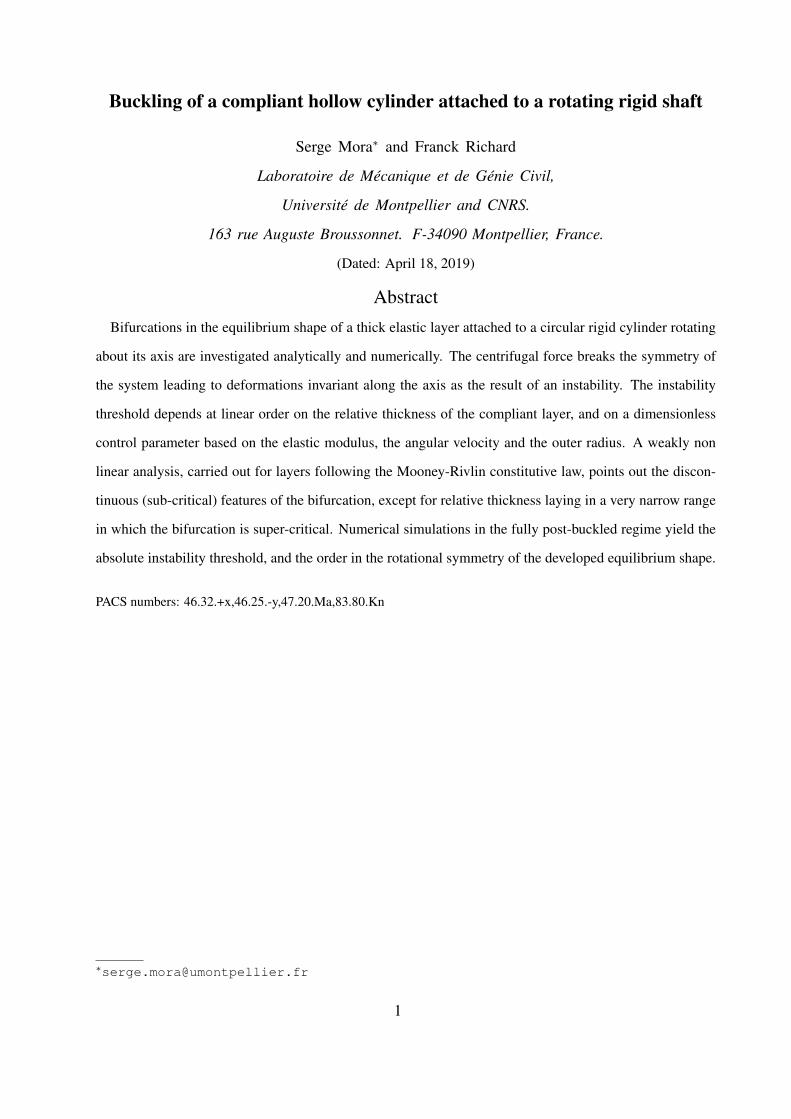
Bifurcations in the equilibrium shape of a thick elastic layer attached to a circular rigid cylinder rotating
about its axis are investigated analytically and numerically. The centrifugal force breaks the symmetry of
the system leading to deformations invariant along the axis as the result of an instability. The instability
threshold depends at linear order on the relative thickness of the compliant layer, and on a dimensionless
control parameter based on the elastic modulus, the angular velocity and the outer radius. A weakly non
linear analysis, carried out for layers following the Mooney-Rivlin constitutive law, points out the discon-
tinuous (sub-critical) features of the bifurcation, except for relative thickness laying in a very narrow range
in which the bifurcation is super-critical. Numerical simulations in the fully post-buckled regime yield the
absolute instability threshold, and the order in the rotational symmetry of the developed equilibrium shape.
PACS numbers: 46.32.+x,46.25.-y,47.20.Ma,83.80.Kn
1

I. INTRODUCTION
Slender pieces can rotate at high angular velocity in mechanical devices such as ultra-
centrifuges, spin-coaters, or high-speed thermal engines. These pieces, made of rigid material
such as metal or composite, are usually cylindrical to avoid unbalance. Connecting pieces be-
tween these rotating rods are often used. For instance, thermal insulators or expansion joints are
placed at the junction between two shafts. In addition, insulators (thermal or electrical) can cover
the rigid shaft to protect it from external disturbances as a sudden increase of the outer temperature
or an unexpected electrical current. These insulators are often polymer-based materials which are
much more compliant than the central shaft. The study of the mechanical behavior of the system
consisting in a rigid right circular cylinder surrounded by a hollow cylinder made in a flexible
elastic material, subjected to high angular velocities, is therefore an important issue for advanced
applications.
Spinning cylinders coated with elastic layers also provides a new route for (micro)patterning,
like designing periodic longitudinal grooves of controlled depth and wavelength at the surface of
cylinders: as shown below, the periodic shape appearing spontaneously at the outer surface can be
controlled by adjusting the layer thickness and the angular velocity (after that, the pattern can be
fixed by initiating a chemical reaction).
Following the pioneering works of Patterson, Haughton and Ogden, and Rabier and Oden [1–
3], bifurcations in the equilibrium shape of homogeneous elastic (solid) cylinders rotating about
their own axis were investigated in a previous article [4], by considering the limit of infinitely
thin central inner rigid rods. At the linear order in terms of the amplitude of the deformations,
these bifurcations were described with a unique dimensionless control parameter α = ρr20ω
2/µ,
with ρ the mass density of the elastic material, µ the shear modulus, r0 the radius and ω the
angular velocity. The linear analysis evidenced an instability threshold at α = 3, leading to a
prismatic deformation of the cylinder (the deformation is invariant under any translation along the
axis) consisting in an ovalization of the cross section with a rotational symmetry of order 2. The
details of the constitutive law of the elastic material were found to be crucial in order to properly
describe the nature of the bifurcation (super-critical or sub-critical) as well as the amplitude of the
deformation and the moment of inertia as a function of the control parameter. It has also been
shown that for any constitutive law, the main features of the bifurcation can be deduced from the
instability of a neo-Hookean elastic cylinder with an apparent shear modulus [4].
2
Here we consider the more common structure consisting in rigid shafts of finite radius, con-
centrically coated with a compliant material, spinning in air about their axis. We first investigate
the linear stability of the elastic cylindrical shell (Sec. III). It is first unstable against a prismatic
deformation beyond a critical angular velocity ωc. ωc depends on the relative thickness of the
layer, on the outer radius, the shear modulus of the compliant layer and its mass density. Then a
weakly non linear analysis addresses the nature of the bifurcation. We demonstrate that depending
on the relative thickness of the elastic layer the transition can be super-critical or sub-critical (Sec.
IV). Finally numerical simulations address the post-buckled regime (Sec. V).
II. EQUILIBRIUM CONDITION
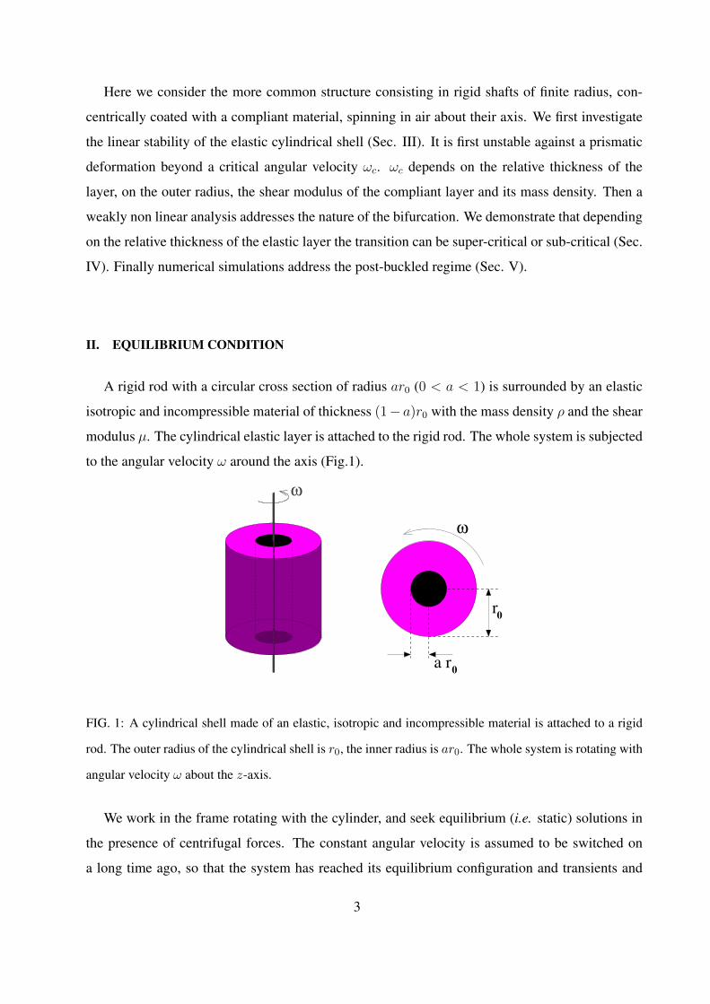
A rigid rod with a circular cross section of radius ar0 (0 < a < 1) is surrounded by an elastic
isotropic and incompressible material of thickness (1− a)r0 with the mass density ρ and the shear
modulus µ. The cylindrical elastic layer is attached to the rigid rod. The whole system is subjected
to the angular velocity ω around the axis (Fig.1).
ω
ω
r0
a r0
FIG. 1: A cylindrical shell made of an elastic, isotropic and incompressible material is attached to a rigid
rod. The outer radius of the cylindrical shell is r0, the inner radius is ar0. The whole system is rotating with
angular velocity ω about the z-axis.
We work in the frame rotating with the cylinder, and seek equilibrium (i.e. static) solutions in
the presence of centrifugal forces. The constant angular velocity is assumed to be switched on
a long time ago, so that the system has reached its equilibrium configuration and transients and
3

other dynamic effects are ignored (transient regimes are assumed to be damped by the dissipa-
tive processes). As a result, this problem is fundamentally different from the classical problem of
‘standing waves’ in tires, which develop when the vehicle reaches a critical velocity; such waves
appear as stationary to an observer moving with the vehicle (hence the somewhat improper name
of ‘standing waves’) but are not stationary in a frame co-rotating with the tire [5–8]. The sym-
metry is broken by the ‘moving’ contact forces with the road and not by an instability. In the
presence of viscoelasticity or any other sources of dissipation, the moving contact forces supply
energy continuously into the system, and no ‘standing waves’ can appear if the contact forces are
removed [9]. By contrast, the elastic bifurcation we study in this paper can take place even in the
presence of viscoelastic dissipation [10], as spinning motion is a rigid-body rotation, even after a
bifurcation has taken place.
In the rotating frame we consider, the equilibrium shape results from the competition between
the elastic force and the centrifugal force, two conservative forces. The static mechanical equilib-
rium is established in a configuration in which the gradient of the potential energy with respect to
the deformation is zero. The deformation of the compliant cylindrical layer is characterized by a
map from the position r of the material in the unbuckled configuration to the spatial position R(r)
in the deformed configuration. For an isotropic and incompressible elastic material, the density
of elastic energy depends on the two first invariants, I1 and I2, of the Green’s deformation tensor
defined as C = FT .F, where F is the deformation gradient (formally, F = ∂R/∂r): I1 = tr C
and I2 = 12
((tr C)2 − tr (C2)
). The elastic energy density can be written as µW (I1, I2) where
W is a dimensionless function depending on the non linear features of the material. µ being the
shear modulus, the dimensionless elastic energy density has to fulfill the condition:
∂W
∂I1
(0, 0) +∂W
∂I2
(0, 0) =1
2. (1)
Incompressibility is imposed by writing that the determinant J of F is equal to one. In order
to characterize equilibrium configurations, the quantity to be minimized with respect to small
variations of the displacement is:
E =
∫
ar0<r<r0; 0<z<h
dr
(µW (I1, I2)− 1
2ρω2
(R ·R− (R · ez)2
)+ µq(J − 1)
). (2)
The first term in the integral is for the strain energy. The second one is for the potential of the
centrifugal force. In the variation, the incompressibility condition, J = 1, is enforced everywhere
by means of the Lagrange multiplier q(r).
4
We consider slender cylinders (h r0) and we focus on the area far from the ends of the cylinders,
i.e. at distances from the cylinder ends significantly larger than r0. Within this hypothesis, for a
fixed value of a and for a given energy density function, the equilibrium of the system is driven by
the unique control parameter
α =ρr2
0ω2
µ. (3)
Rr
Θθ
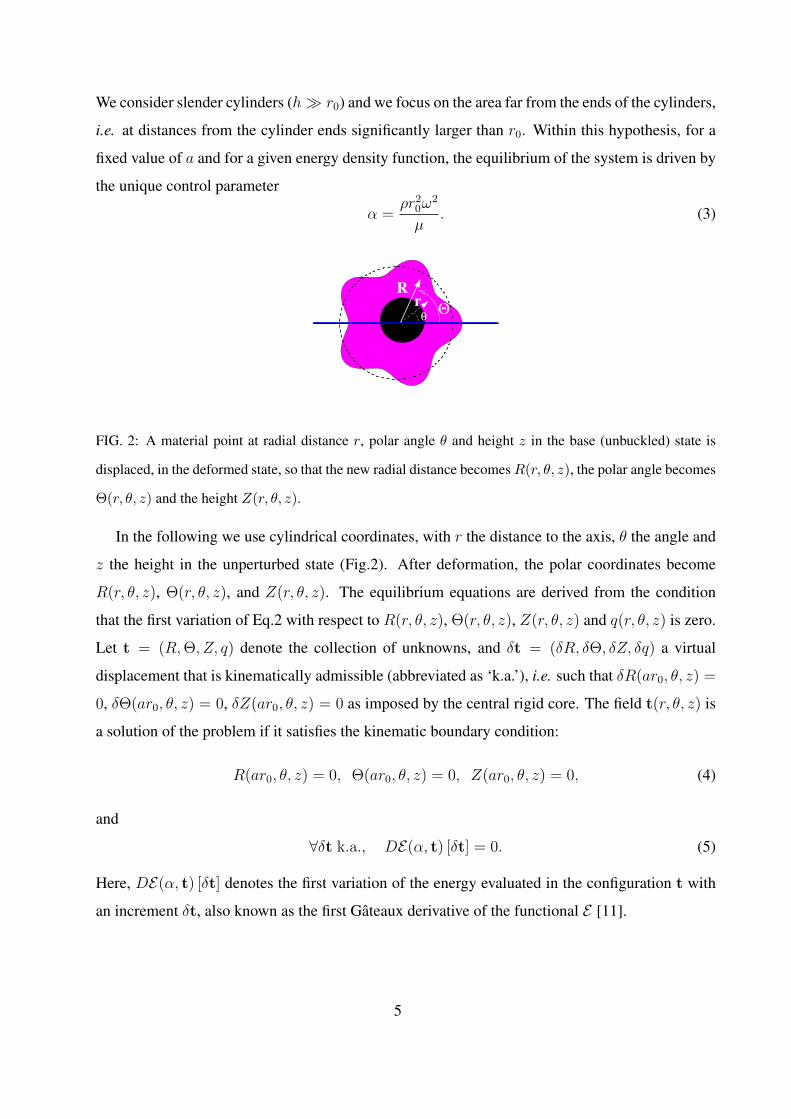
FIG. 2: A material point at radial distance r, polar angle θ and height z in the base (unbuckled) state is
displaced, in the deformed state, so that the new radial distance becomesR(r, θ, z), the polar angle becomes
Θ(r, θ, z) and the height Z(r, θ, z).
In the following we use cylindrical coordinates, with r the distance to the axis, θ the angle and
z the height in the unperturbed state (Fig.2). After deformation, the polar coordinates become
R(r, θ, z), Θ(r, θ, z), and Z(r, θ, z). The equilibrium equations are derived from the condition
that the first variation of Eq.2 with respect to R(r, θ, z), Θ(r, θ, z), Z(r, θ, z) and q(r, θ, z) is zero.
Let t = (R,Θ, Z, q) denote the collection of unknowns, and δt = (δR, δΘ, δZ, δq) a virtual
displacement that is kinematically admissible (abbreviated as ‘k.a.’), i.e. such that δR(ar0, θ, z) =
0, δΘ(ar0, θ, z) = 0, δZ(ar0, θ, z) = 0 as imposed by the central rigid core. The field t(r, θ, z) is
a solution of the problem if it satisfies the kinematic boundary condition:
R(ar0, θ, z) = 0, Θ(ar0, θ, z) = 0, Z(ar0, θ, z) = 0, (4)
and
∀δt k.a., DE(α, t) [δt] = 0. (5)
Here, DE(α, t) [δt] denotes the first variation of the energy evaluated in the configuration t with
an increment δt, also known as the first Gateaux derivative of the functional E [11].
5

III. LINEAR ANALYSIS
For the linear stability analysis, we deal with a small perturbation εt1 of the base solution:
t = t0 + εt1 = (r + εu1(r, θ, z), θ + εΘ1(r, θ, z), z + εz1(r, θ, z), q0 + εq1(r, θ, z)) . (6)
Eq.5 writes at order ε0:
DE(α, t0)[δt] = 0, (7)
and at order ε:
D2E(α, t0)[δt, t1] = 0, (8)
where D2E is the second Gateaux derivative of E , which is a bi-linear form on the increment t1
and on the virtual increment δt.
From Eq.7 one obtains (see [4]):
q0 =α
2
(1− (r/r0)2
)− 1. (9)
In order to deal with order ε, Eq.8, we assume in a standard way a harmonic θ and z dependence
of any variation of the perturbation of R, Θ, Z and q:
u1(r, θ, z) = Re(fu(r)e
inθ+ikz)
Θ1(r, θ, z) = Re(−ifΘ(r)einθ+ikz
)
z1(r, θ, z) = Re(−ifz(r)e
inθ+ikz)
q1(r, θ, z) = Re(fq(r)e
inθ+ikz)
(10)
where Re denotes the real part. The conventional complex factor (−i) has been included for
convenience, anticipating the fact that the phase of Θ1 and z1 is shifted by π/2 compared to
the phase of the other two unknowns. n is the circumferential wave number and k is the axial
wave number. Since R(r, θ, z) = R(r, θ + 2π, z), n has to be an integer. Furthermore, from the
symmetries θ ↔ −θ and z ↔ −z, one can take n and k positive.
In a previous paper [4] dealing with homogeneous spinning (solid) cylinders (a → 0) we have
shown that fu(r) is a solution of the linear differential equation for fu of order 6:(r6 d2
dr2+ 7r5 d
dr− r4
(k2r2 + n2 − 4n− 5
))L2fu = 0, (11)
where
L =d2
dr2+
1
r
d
dr−(k2 +
(n+ 1)2
r2
), (12)
6

with three boundary conditions at r = r0. In the presence of a rigid inner shaft of finite radius ar0,
one has to deal with the three additional kinematic boundary conditions at r = ar0 given by Eqs.4.
For a fixed value of the circumferential wave number n, the solutions of Eq.11 can be written as a
generalized series expansion
fu(r) =∞∑
m=−∞(am + bm ln(kr)) (kr)m, (13)
where am and bm depends on the circumferential wave number. For each n, the sequence
(am, bm)m is determined up to six unknown values, that are fixed by the six boundary conditions.
Non zero solutions (i.e. (am, bm)m 6= 0) exist only for particular values of α that depends on the
circumferential wave number n and on the wave number k, α = αc(n, k) as detailed in Appendix
B. For α = αc(n, k) the straight system is neutrally stable against an infinitesimal perturbation of
circumferential wave number n and axial wave number k.
αc(0, k), αc(1, k), αc(2, k), αc(3, k) are plotted as a function of k in Fig.3 for different values
of the dimensionless inner radius a. For n = 0 the linear instability threshold αc(n = 0, k) is
minimal for a finite k, and for n > 0 and for any a, the linear instability threshold is an increasing
function of k. For any a, the absolute minimal value of αc(n, k) (as a function of n and k) is
minimal for a given value of n, n = nfirst, and k = 0 (Fig.4). One concludes that the lower αc(n, k)
is for a prismatic deformation (k = 0). Therefore, if one focuses on the first mode that develops
upon increasing values of α, one can limit the study to plane-strain deformations. Accordingly,
throughout the rest of the article, the wave number is fixed to k = 0 and the explicit dependence
of any quantity with respect to k is dropped. Taking k = 0 (or equivalently ∂∂z
= 0) in the linear
analysis, Eq.11 simplifies in [4]:
(n2 − 1
)2fu −
(2n2 + 1
)r
dfudr
+(5− 2n2
)r2 d2fu
dr2+ 6r3 d3fu
dr3+ r4 d4fu
dr4= 0, (14)
whose general solution is:
fu = r0
(A
(r
r0
)n+1
+B
(r
r0
)n−1
+ C
(r
r0
)1−n+D
(r
r0
)−n−1)
for n 6= 1, (15)
fu = r0
(A
(r
r0
)2
+B + C ln
(r
r0
)+D
(r
r0
)−2)
for n = 1, (16)
where A, B, C and D are four constants. With the boundary conditions, one obtains the analytic
expression of the linear instability threshold α = αc(n) as a function on the circumferential mode
7

a = 0.5a = 0.4a = 0.3a = 0.2a = 0.1a = 0
kr0
αc(n=
0,k)
.
54321
14
12
10
8
6
4a = 0.5a = 0.4a = 0.3a = 0.2a = 0.1
a = 10−5
kr0
αc(n=
1,k)
.
54321
10
9
8
7
6
5
4
3
2
1
0
a = 0.5a = 0.4a = 0.3a = 0.2a = 0.1a = 0
kr0
αc(n=
2,k)
.
54321
11
10
9
8
7
6
5
4
3a = 0.5a = 0.4a = 0.3a = 0.2a = 0.1a = 0
kr0
αc(n=
3,k)
.
543210
11
10
9
8
7
6
5
FIG. 3: Critical load parameter for the modes (n, k) at the instability threshold, αc(n, k), as a function of
the dimensionless wave number, kr0, for the circumferential wave numbers n = 0, 1, 2, 3 and for various
values of the relative radius of the inner cylinder, a.
n and on parameter a (see Appendix A):
αc(n) =
(2(n+ 1)(n− 1)
n
)(n2a2n(a2 − 1)2 + a2(a2n + 1)2
na2n(a4 − 1) + a2(1− a4n)
)for n > 1, (17)
αc(1) =8
a4−1a4+1− 2 ln(a)
for n = 1. (18)
Fig.4-left shows for various values of parameter a and for different circumferential modes n,
the critical load αc so that mode n is neutrally unstable. Note that αc(1) for a = 0 does not lead to
a buckled configuration, as it can be anticipated from Eq.16 in which the displacement diverges at
r = 0. This point will be enlightened in Sec. IV.
8

a=0.6
a=0.4
a=0.2
a=0
n
αc(n)
.
7654321
16
14
12
10
8
6
4
2
0
a
nfirst
alinear5
alinear4
alinear3
alinear2
10.80.60.40.20
100
20
10
2
1
a
αc(n
first)
.
10.80.60.40.20
1000
100
10
1
FIG. 4: Left: Critical load αc(n) making the prismatic mode n neutrally unstable, for different values of the
dimensionless inner radius a. Right: Value of the circumferential wave number n making αc(n) minimal,
for a given value of a. Inset: Threshold value of the load parameter beyond which a mode is unstable, as a
function of a.
For a given value of a, we call nfirst the circumferential wave number n minimizing the critical
load αc(n). It follows that the instability is expected (from the linear analysis) to first appear for
α = αc(nfirst). The circumferential wave number nfirst is a discontinuous function of a; it increases
step by step as a increases (Fig.4-right). Reciprocally, one defines the sequence (alinearn )n so that
nfirst = n for a ∈ [alinearn , alinear
n+1] (inset of Fig.4). The instability threshold for the prismatic mode with
a circumferential wave number n = 1 is the lowest if αc(1) < αc(2), which defines (from Eqs.18
and 17) the critical value of a, alinear2 ' 0.218, below which the first mode to appear is, at linear
order, n = 1 (nfirst = 1). alinear3 is defined in the same way by αc(2) = αc(3), alinear
3 ' 0.420: for
alinear2 < a < alinear
3 the first mode to be linearly unstable is the mode with a rotational symmetry of
order 2 (invariant under a central rotation of π), nfirst = 2. The whole sequence (alinearn )n is defined
as well.
In this section, we have shown that the instability first appears, upon increasing values of the
load parameter α, for prismatic modes. The linear instability threshold is for α = αc(nfirst), where
the function αc(n) is defined by Eqs.18 and 17. The value of nfirst depends on the relative radius
a of the inner cylinder: the critical radius separating nfirst − 1 to nfirst, alinearn , is determined by the
condition αc(nfirst − 1) = αc(nfirst).
9
In the next section, a weakly non linear analysis is carried out in order to capture the amplitude
of the buckled modes as a function of the load parameter close to the linear thresholds.
IV. WEAKLY NON LINEAR ANALYSIS
A. Post-bifurcation expansion
Both the load parameter α and the solution t = (R,Θ, q) are expanded in terms of the small
arc-length parameter ε as:
α = αc + α2ε2 (19)
t(α) = t0(α) + εt1 + ε2t2 + ε3t3 + · · · (20)
where αc = αc(n) is the critical load from the linear bifurcation analysis (see Eqs.18 and 17), and
t1 is the corresponding linear mode. In the following, the dependence of αc on n will become
implicit in our notation, for the sake of readability. Note that the base solution t0 depends on the
load α through the pressure parameter q0. The first-order correction t1 is the linear mode from
Section III. The asymptotic post-buckling expansion method [12–18] proceeds by inserting the
expansion in Eqs.19–20 into the non linear equilibrium written earlier in Eq.5 as
∀δt k.a., DE(αc + α2ε
2, t0(α) + εt1 + ε2t2 + ε3t3 + · · ·)
[δt] = 0, (21)
where δt(r, θ) is the set of virtual functions(δR, δΘ, δq
)that represent infinitesimal increments
satisfying the kinematic boundary conditions. Equation 21 is then expanded order by order in
ε [4, 18–20]. At order ε2, we obtain an equation for t2,
∀δt k.a., D2E(αc, t0(αc)) · [t2, δt] + 12D3E(αc, t0(αc)) · [t1, t1, δt] = 0. (22)
At order ε3, one obtains the equation
∀ k.a.δt, D2E(αc, t0(αc)) · [t3, δt] +D3E(αc, t0(αc)) · [t2, t1, δt] · · ·
+ α2dD2E(α, t0(α))
dα
∣∣∣∣α=αc
· [t1, δt] +1
6D4E(αc, t0(αc)) · [t1, t1, t1, δt] = 0.
Upon insertion of the particular virtual displacement δt = t1, the first term cancels out by Eq.8
and we are left with
D3E(αc, t0(αc))·[t2, t1, t1]+α2dD2E(α, t0(α))
dα
∣∣∣∣α=αc
·[t1, t1]+1
6D4E(αc, t0(αc))·[t1, t1, t1, t1] = 0.
(23)
10
In the equations above, D2E [δt; t1] denotes the second Gateaux derivative of E , which is a
bi-linear symmetric form on the increment t1 and on the virtual increment δt. Similarly,
D3E [δt; t1; t2] is the third Gateaux derivative (a tri-linear symmetric form).
B. Second order correction to the displacement
The second order displacement t2 = (u2,Θ2, q2) can be computed from Eq.22 with the already
known expressions of t0 and t1. t1 = (u1,Θ1, q1) is fixed up to a multiplicative constant that
defines the buckling amplitude at linear order (Sec. III). In the following, this constant is chosen
so that the amplitude of u1 is ξ:
u1(r0, θ) = ξ cos(nθ). (24)
Eq.23 will be used later (in Sec.IV C) in order to fix the amplitude ξ.
Since t2 = (u2,Θ2, q2) results from the non linear coupling of the linear mode t1 with itself
(Eq.22), it can be expressed as
u2 = gu(r) +Re(gu(r)e
2inθ), (25)
Θ2 = gΘ(r) +Re(−igΘ(r)e2inθ
), (26)
q2 = gq(r) +Re(gq(r)e
2inθ), (27)
where gu, gΘ and gq are second order complex amplitudes that are functions of r only, and gu, gΘ
and gq represent the constant terms in u2, Θ2 and q2 respectively, which are also functions of r.
Inserting the expressions t0 and t1 in Eq.22, one obtains in strong form a set of seven equa-
tions: the incompressibility constraint, the equilibrium in the radial and circumferential directions,
the kinematic condition at r = ar0 and the boundary equations at r = r0, in the radial and cir-
cumferential directions. Each equation can be separated in two parts : one is independent of θ
and involves gu, gΘ and gq. The other part depends on θ and involves gu, gΘ and gq. The deriva-
tion as well as the resolution of these equations are detailed in Appendix C for an isotropic and
incompressible neo-Hookean material for which, in the plane-strain problem we consider here,
W = 1/2 (I1 − 3).
In the following, we focus on materials that follow this constitutive law. Note that for an
incompressible material, the neo-Hookean model is equivalent to the Mooney-Rivlin constitutive
law in plane-strain deformation [21]. This study is therefore also relevant for any incompressible
Mooney-Rivlin solid.
11

C. Determination of the amplitude of mode n
D2E(α, t0(α)) · [t1, t1], D3E(αc, t0(αc)) · [t2, t1, t1] and D4E(αc, t0(αc)) · [t1, t1, t1, t1] are
calculated with the help of a symbolic calculation language and without any approximation, as a
function of r0, a, n and ξ from the expressions of fu, fΘ, fq, gu, gq, gΘ, gu, gq and gΘ introduced in
Sections III and IV. Since t1 is proportional to ξ and t2 is proportional of ξ2, the second Gateaux
derivative aforementioned is proportional to ξ2, the third and the fourth Gateaux derivative in
Eq.23 are proportional to ξ4. One obtains from Eq.23 a relation between ξ, a, n and α2 in the
form: (ξ
r0
)2(α2 − fn(a)
(ξ
r0
)2)
= 0, (28)
with fn(a) a function of a whose exact expression is too cumbersome to be written here. f1(a)
and f2(a) are plotted in Fig.5. fn(a) is plotted in Fig.6 for n = 1, ..., 6 together. f1 is negative for
a
f 1(a)
.
mode n = 1 is super-criticalcritical
is sub-
mode n = 1
a+110.80.60.40.20
50
25
0
-25
a
f 2(a)
.
super-critical
mode n = 2 is
critical
is sub-
mode n = 2
critical
is super-
mode n = 2
a+2a−210.80.60.40.20
100
75
50
25
0
-25
-50
FIG. 5: f1 (left) and f2 (right) as a function of a, calculated from the analytic expressions deduced from
Eq.23.
a in the range [0, a+1 ] with a+
1 ' 0.218. Then f1 is positive and change again of sign for a close
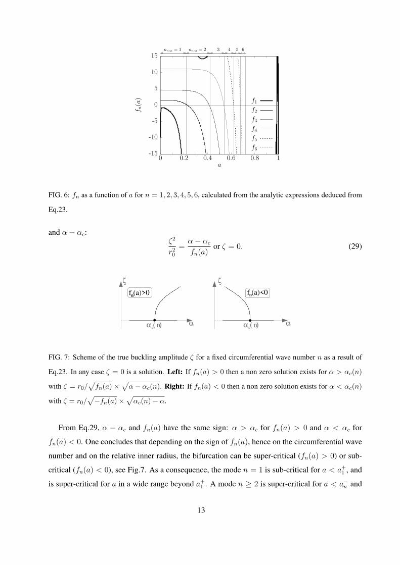
to 1 (see Fig.5(left)). The variations of functions fn(a) have the same structure than f2(a) for any
n > 1 (see Fig.6): fn(a) is positive in the range [0, a−n ] with a−n ∈]0, 1[. It is negative in [a−n , a+n ].
It is then positive until a value of a close to 1. In Fig.6 the vertical axis is zoomed in order to focus
on the first zero of the functions fn.
We define the true buckling amplitude ζ as the amplitude of the displacement R− r. At linear
order, ζ = ε ξ. With Eqs.19, 24 and 20, one obtains from Eq.28 the relation (at order ε) between ζ
12
f6
f5
f4
f3
f2
f1
a
f n(a)
.6543nfirst = 2nfirst = 1
10.80.60.40.20
15
10
5
0
-5
-10
-15
FIG. 6: fn as a function of a for n = 1, 2, 3, 4, 5, 6, calculated from the analytic expressions deduced from
Eq.23.
and α− αc:ζ2
r20
=α− αcfn(a)
or ζ = 0. (29)
cα ( )n αα α ( )
cn
ζ ζ
nf (a)>0 nf (a)<0
FIG. 7: Scheme of the true buckling amplitude ζ for a fixed circumferential wave number n as a result of
Eq.23. In any case ζ = 0 is a solution. Left: If fn(a) > 0 then a non zero solution exists for α > αc(n)
with ζ = r0/√fn(a) ×
√α− αc(n). Right: If fn(a) < 0 then a non zero solution exists for α < αc(n)
with ζ = r0/√−fn(a)×
√αc(n)− α.
From Eq.29, α − αc and fn(a) have the same sign: α > αc for fn(a) > 0 and α < αc for
fn(a) < 0. One concludes that depending on the sign of fn(a), hence on the circumferential wave
number and on the relative inner radius, the bifurcation can be super-critical (fn(a) > 0) or sub-
critical (fn(a) < 0), see Fig.7. As a consequence, the mode n = 1 is sub-critical for a < a+1 , and
is super-critical for a in a wide range beyond a+1 . A mode n ≥ 2 is super-critical for a < a−n and
13

sub-critical for a−n < a < a+n .
A summary list of the critical inner radii introduced above, with their definition, is provided in
Appendix D.
D. Discussion
We focus on the transition from the unbuckled to the first buckled configuration, i.e. on the
first mode that appears upon increasing values of α. Interesting features of the bifurcation (as the
instability threshold and the critical nature of the transition) can be deduced from the comparison
of the sequences (a−n )n, (a+n )n and (alinear
n )n. Note that for a reason that is unclear for us, a+1 = alinear
2 .
• For dimensionless radius a < a+1 ' 0.218, f1(a) < 0 and fn(a) > 0 for any circumferential
wave number n > 2 (Fig.8). Modes with n ≥ 2 will therefore not develop first since they
appear for a load α > αc(n) > αc(1). From the negative sign of f1(a) we deduce that the
bifurcation is sub-critical with the true buckling amplitude ζ = r0√−f1(a)
√αc(1)− α (Fig.9-
a). Note that for a = 0, the unique solution of Eq.28 is ξ = 0 since α2 is in this case always
positive (αc(1) = 0).
• Let us consider systems with a thinner compliant layers, the relative radius a being such
that a+1 < a < a−2 ' 0.228. In this case fn(a) > 0 for any n (Fig.8) and the bifurcation
is super-critical. Since in this range of a, nfirst = 2, the mode with a rotational symmetry of
order 2 develops first with the true buckling amplitude ζ = r0√f2(a)
√α− αc(2) (Fig.9-b).
• For systems with a such that a−2 < a < a−3 ' 0.414, nfirst = 2, f2(a) < 0 and fn6=2(a) > 0
(Fig.8). One concludes that the bifurcation is sub-critical and appears with mode n = 2.
• For systems with a such that a−3 < a < a+2 ' 0.478, f2(a) < 0, f3(a) < 0 and the
others fn(a) are positive (Fig.8). Moreover nfirst = 2 or nfirst = 3. The bifurcation is then
sub-critical and appears either with mode n = 2 or mode n = 3. One cannot discriminate
between n = 2 or n = 3 from the weakly non linear analysis (Fig.9-c and Fig.11).
• For systems with a such that a+2 < a < a−4 ' 0.538, nfirst = 3, f3(a) < 0, fn 6=3(a) > 0
(Fig.8). The bifurcation is therefore sub-critical and the mode n = 3 develops (Fig.9-d).
• For systems with a such that a−4 < a < a+3 ' 0.612, f3(a) < 0, f4(a) < 0 and the other
fn(a) are positive (Fig.8). In this case nfirst = 3 or nfirst = 4: the bifurcation is sub-critical
14
2 3a a a
0.2
28065
0.4
13805
0.4
20453
a3
a a a a− −
a
a6
0.6
79123
a6
−
0.6
78793
5
0.6
22549
5
0.6
20323
−
a3
+
0.6
12261
linear
4
0.5
42288
4
−
0.5
37463
2
+
0.4
78496
firstn =4
first
linear linear linear
n =3first
n =5
mode 2sub−
critical
modes 2 and 3
criticalsub−
mode 3
criticalsub−
modes 3 and 4
sub−critical
mode 4sub−
critical
modes 4 and 5sub−critical sub−
modes 4,5,6critical
super−critical super−critical
(c) (d) (e) (f)
n =2firstfirstn =1
a2
linear
1a+
0.2
18047
criticalsub−
mode 1
criticalsuper−
modes 1 and 2 mode 1
super−criticalmodes 1 and 2 modes 1, 2 and 3
(a) (b)
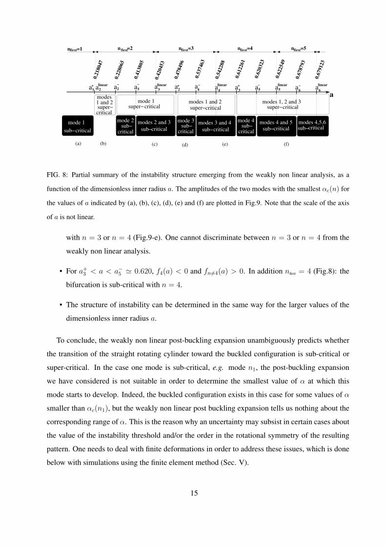
FIG. 8: Partial summary of the instability structure emerging from the weakly non linear analysis, as a
function of the dimensionless inner radius a. The amplitudes of the two modes with the smallest αc(n) for
the values of a indicated by (a), (b), (c), (d), (e) and (f) are plotted in Fig.9. Note that the scale of the axis
of a is not linear.
with n = 3 or n = 4 (Fig.9-e). One cannot discriminate between n = 3 or n = 4 from the
weakly non linear analysis.
• For a+3 < a < a−5 ' 0.620, f4(a) < 0 and fn6=4(a) > 0. In addition nfirst = 4 (Fig.8): the
bifurcation is sub-critical with n = 4.
• The structure of instability can be determined in the same way for the larger values of the
dimensionless inner radius a.
To conclude, the weakly non linear post-buckling expansion unambiguously predicts whether
the transition of the straight rotating cylinder toward the buckled configuration is sub-critical or
super-critical. In the case one mode is sub-critical, e.g. mode n1, the post-buckling expansion
we have considered is not suitable in order to determine the smallest value of α at which this
mode starts to develop. Indeed, the buckled configuration exists in this case for some values of α
smaller than αc(n1), but the weakly non linear post buckling expansion tells us nothing about the
corresponding range of α. This is the reason why an uncertainty may subsist in certain cases about
the value of the instability threshold and/or the order in the rotational symmetry of the resulting
pattern. One needs to deal with finite deformations in order to address these issues, which is done
below with simulations using the finite element method (Sec. V).
15

α
ζ/r
0
n=3
n=2
.
9.89.69.49.298.88.68.4
0.2
0.15
0.1
0.05
0
α
ζ/r
0
n=
3
n = 2
.
7.0427.047.0387.0367.0347.032
0.05
0.04
0.03
0.02
0.01
0
α
ζ/r
0
n=4
n=
5
.
14.6514.614.5514.514.4514.414.3514.314.25
0.08
0.07
0.06
0.05
0.04
0.03
0.02
0.01
0
α
ζ/r
0
n=3
n=4
.
12.612.412.21211.8
0.1
0.08
0.06
0.04
0.02
0
α
ζ/r
0
n=
2n=1
.
3.43.33.23.132.92.82.72.6
0.25
0.2
0.15
0.1
0.05
0
α
ζ/r
0
n=
2
n = 1
.
3.963.9553.953.9453.943.9353.933.9253.923.915
0.08
0.07
0.06
0.05
0.04
0.03
0.02
0.01
0
(d)(c)
(f)(e)
(a) (b)
FIG. 9: Amplitudes ζ of modes of deformation as a function of the load parameter α, for different rela-
tive radius of the inner cylinder (values of a are 0.15, 0.22, 0.42, 0.5, 0.6, 0.65 in figs (a), (b), (c), (d),
(e) and (f) respectively). Solid lines are for amplitudes computed from the analytic expression Eq.29.
Empty circles and the snapshots originate from finite element simulations of Section V. The amplitude of
the unstable mode with the lowest value of αc is in black (circumferential wave numbers are respectively
nfirst = 1, 2, 2, 3, 4 and 5), and the amplitude of the second mode with the lowest value of αc is in gray
(circumferential wave numbers are respectively n = 2, 1, 3, 2, 3 and 4). The other modes are not shown in
these figures. Deformed shapes obtained by simulations are shown in the insets ; the color map represents
the magnitude of the displacement increasing from blue (no displacement) to orange.16
V. BEYOND THE WEAKLY NON LINEAR ANALYSIS
In this section we numerically implement the complete non linear problem defined by Eq.5 by
using the open source tool for solving partial differential equations FEniCS [22]. In a first step,
we show that the numerical simulations that we have implemented capture well the results of the
linear analysis and the non linear analysis (Sec. V A). Then we present the results obtained beyond
the validity range of the weakly non linear analysis (Sec. V B).
A. Finite element implementation
We consider a 2-dimensional corona Ωa of inner and outer radii equal respectively to ar0 and
r0 (0 < a < 1). A Cartesian coordinates system (x, y) with the base vectors (ex, ey) is chosen
such that (x, y) ∈ Ωa ⇔ a < r/r0 < 1, with r =√x2 + y2. An incompressible and isotropic
neo-Hookean elastic solid occupying the domain Ωa in its reference configuration is subjected to
the action of the centrifugal volume force α(xex + yex)/r. The inner surface is prescribed to have
zero displacement and the outer one is traction free. The non linear problem in u − q, with u the
displacement vector and q the Lagrange multiplier, is solved using a Newton algorithm based on
a direct parallel solver (MUMPS). Quasi-static simulations are performed by setting µ = 1, r0 = 1,
and slowly varying α up to the desired value. For each α the displacement field, the Lagrange
multiplier and the total energy of the system (taking for the energy reference the base state ) are
computed.
Starting from the undisturbed system (u = 0), α is gradually increased or decreased (with
increments δα = 1/4000). A spatially uncorrelated random disturbance of maximal amplitude
ξ0 = 10−3 is added before each step in order to trigger the instability. Due to its small amplitude,
the random disturbance no longer plays a role once the instability has begun to develop. Simula-
tions have been carried out for different values of the relative inner radius a and different values
of the linear mesh density nmesh. Depending on the initial value of α, on a and on nmesh the
instability develops below (as in Figs. 9-a,c,d,e,f) or beyond (as in Figs. 9-a,b,d) a critical load
α∗(nmesh). The convergence of α∗(nmesh) with the linear mesh density nmesh is shown in Fig.10
for a = 0.44. The limit α∗(nmesh → ∞) is consistent with the analytical prediction (Eqs.18 and
17), with a residual error well below 10−4.
The true buckling amplitude ζ defined in Sec. IV C, i.e. the amplitude of the displacement
17
R− r, is computed from the simulations as ζ = 12(Rmax/Rmin − 1), where Rmin and Rmax are
the smallest and largest distance from the deformed lateral boundary to the origin. This amplitude
ζ is plotted as a function of α in Figs. 9 for different values of a, and compared to the prediction
based on the weakly non linear post buckling expansion (Eqs.29). The agreement is good in the
limit of the small amplitudes, which indeed corresponds to the domain of validity of the post-
buckling expansion.
1/nmesh
α∗ /αc(2)
.
0.050.040.030.020.010
1
0.9995
0.999
0.9985
0.998
nmesh = 200nmesh = 100nmesh = 40nmesh = 20
α− α∗(nmesh)
ζ/r
0
.
10−110−210−310−4
10−1
10−2
10−3
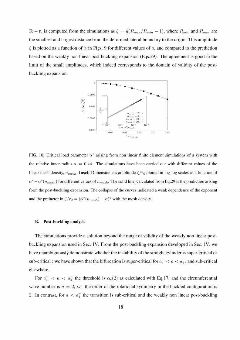
FIG. 10: Critical load parameter α∗ arising from non linear finite element simulations of a system with
the relative inner radius a = 0.44. The simulations have been carried out with different values of the
linear mesh density, nmesh. Inset: Dimensionless amplitude ζ/r0 plotted in log-log scales as a function of
α∗−α∗(nmesh) for different values of nmesh. The solid line, calculated from Eq.29 is the prediction arising
form the post-buckling expansion. The collapse of the curves indicated a weak dependence of the exponent
and the prefactor in ζ/r0 = (α∗(nmesh)− α)p with the mesh density.
B. Post-buckling analysis
The simulations provide a solution beyond the range of validity of the weakly non linear post-
buckling expansion used in Sec. IV. From the post-buckling expansion developed in Sec. IV, we
have unambiguously demonstrate whether the instability of the straight cylinder is super-critical or
sub-critical : we have shown that the bifurcation is super-critical for a+1 < a < a−2 , and sub-critical
elsewhere.
For a+1 < a < a−2 the threshold is αc(2) as calculated with Eq.17, and the circumferential
wave number is n = 2, i.e. the order of the rotational symmetry in the buckled configuration is
2. In contrast, for a < a+1 the transition is sub-critical and the weakly non linear post-buckling
18

expansion is not enough to find the lower value of α at which an unstable mode first exists. Note
that in this case the only mode that will first occur consists in a continuation of mode n = 1 since
the other modes (n = 2, 3, 4, ...) are super-critical with a larger linear threshold. For a−3 < a < a+2 ,
both modes n = 2 and n = 3 are sub-critical, and then one does not know which one of these
two modes appears first. For a+2 < a < a−4 , mode n = 3 is sub-critical ; the other modes are
super-critical and then, the order of the rotational symmetry in the buckled configuration is 3.
α
1 2
(R
max
Rm
in−1)
.
αm(2) αc(3)
αc (2)
n=3
n = 2
.
7.87.67.47.276.8
1.2
1
0.8
0.6
0.4
0.2
0
α
E tot/(µr2 0h)
αm(2)
αc (3)
αc (2)
n=3
n = 2
a = 0.44
.
7.87.67.47.276.8
0.05
0.04
0.03
0.02
0.01
0
−0.01
−0.02
FIG. 11: Left - True buckling amplitude ζ as a function of the load parameter α for a = 0.44 computed
for deformations with rotational symmetry of order n = 2 and n = 3, which corresponds to the two lowest
values of α at the linear threshold. Since for this value of a the modes with circumferential wave numbers
n = 2 and n = 3 are sub-critical, the buckled configurations start to develop bellow the linear thresholds,
respectively αc(2) and αc(3). Deformed shapes obtained by simulations are shown in the insets ; the color
map represents the magnitude of the displacement increasing from blue (no displacement) to orange. Right
- Dimensionless energy of the system as a function of α.
In the following, we use finite element simulations beyond the domain of validity of the weakly
non linear post-buckling expansion in order to determine the lowest value of α for which the
instability occurs (for a given value of a) through the hypothesis of plane-strain deformations. Let
us consider a value of a so that the bifurcation is sub-critical. Upon decreasing α from the linear
threshold toward lower values, the computed true amplitude ζ of a mode with rotational symmetry
of order n increases as well as the associated energy (Fig.11), until a particular value of α at which
the slope of ζ versus α is infinite. We call αm(n) the corresponding value of α. No buckled
solution is found for α < αm(n). Increasing now α from αm(n) toward larger values, the true
buckling amplitude ζ again increases. The total energy is found to increase as α decreases during
19

αm
αc(nfirst)
a
α
n = 3
n = 2
n = 1
a+2a−2
alinear2 alinear4alinear3
0.60.50.40.30.20.10
10
8
6
4
2
0
FIG. 12: Instability threshold as a function of a, considering deformations with rotational symmetry of
order 1 (n = 1, magenta), order 2 (n = 2, blue) and order 3 (n = 3, red) for a in the range [0.05, 0.58].
Filled circles are for the minimal value of α, αm, for which a buckled solution exists. Continuous lines are
for αc(nfirst) calculated from Eqs.18 and 17.
the first step (from α∗(nmesh) to αm), and to decrease as α increases beyond αm in the second step,
reaching negative values beyond a certain α > αm(n) (Fig.11-right). The solutions corresponding
to the first step (from α∗(nmesh) to αm) are unstable, while the solutions corresponding to the
second step (α increases beyond αm) are stable [4, 23, 24].
As a consequence, even if the energy is positive, i.e. higher than the energy of the base state,
a stable buckled solution exists for α > αm. αm(n) is the lowest possible value of the load
parameter α for a non zero solution with a rotational symmetry of order n. If now the rotational
symmetry n corresponds to a supercritical mode, the lowest value of α so that de deformation with
this symmetry develops is obviously αm(n) = αc(n).
For a fixed value of the dimensionless inner radius a, the first deformation that can develop
is therefore the deformation with the rotational symmetry of order n having the lowest αm(n).
For example in Fig.11 where a = 0.44, one observes that, even if αc(2) > αc(3) (i.e. nfirst =
3), αm(3) > αm(2): the order in the rotational symmetry of the deformation that appears upon
increasing α is therefore 2. For given values of a, a systematic comparison of αm(n) for different
n yields the absolute instability threshold, αm, of the system. αm is plotted as a function of a
together with αc(nfirst) in Fig.12, for a in the range [0.05, 0.58]. αm is smaller than αc(nfirst) except
for a ∈ [alinear2 , a−2 ] since the instability is super-critical in this case. The order in the rotational
20
symmetry is equal to n = 1 for 0 < a < alinear2 , it is equal to n = 2 for a−2 < a < a+
2 : the uncertainty
over the order in the rotational symmetry for a−3 < a < a+2 is then now fixed. Strikingly, the
absolute threshold αm is not a continuous function of a, since one observes a jump for a = alinear2
and a = a+2 .
The different critical control parameters α defined above are summarized, together with the critical
inner radii, in Appendix D.
VI. CONCLUDING REMARKS
The bifurcations in cylinders consisting in a rigid shaft surrounded by an homogeneous and
incompressible elastic hollow cylinder rotating about their axis, have been investigated. They
arise at critical load parameters that depend on the geometry (through the relative radius of the
rigid shaft, a), on the mass density of the hollow cylinder, its shear modulus, and the angular
velocity square.
The complete linear analysis shows that this 3-dimensional system can be reduced, for the
weakly non linear regime, to a plane-strain formulation. While the stability analysis we propose
is valid for any elastic constitutive law, our weakly non linear analysis has been carried out
for a Mooney-Rivlin constitutive law for the sake of simplicity, which exactly coincides to the
neo-Hookean form in this plane-strain problem. As a consequence, the unique relevant elastic
parameter is the shear modulus µ, and no additional material constant is needed. Within this
hypothesis, the bifurcation is super-critical for systems with 0.218 < a < 0.228, and sub-critical
elsewhere. The corresponding buckling amplitude has been calculated at order |α−αc|1/2, with αc
the critical load parameter calculated from the linear analysis and α the actual load parameter. The
agreement with finite element simulations is excellent. In case of sub-critical bifurcations leading
to configurations with rotational symmetry of order n, a weakly non linear analysis cannot predict
the lowest possible value of the load parameter (αm(n)) at which these buckled configurations can
develop, because the corresponding deformations are finite. αm(n) has then been computed by
means of finite element simulations. For a given value a of the relative inner radius, minimizing
αm(n) with respect to n gives the lowest load parameter for a buckled configuration, with the
corresponding order n of the rotational symmetry.
Indeed, the buckling amplitude as well as the range in which the bifurcation is super/sub-
21
critical depend on the precise constitutive law that may deviate from the Mooney-Rivlin model for
certain rubber-like materials. Following [4], one postulates that the post-buckling behavior of such
system with an arbitrary elastic constitutive law for the elastic hollow cylinder can be captured, at
least qualitatively, by replacing the modulus µ in the prediction of the neo-Hookean model by the
apparent modulus µapp defined (for plane-strain deformations) as:
µapp(I1) = 2µW (I1)
I1 − 3, (30)
where µapp is evaluated for I1 = 〈I1〉, the mean value of the first invariant I1 calculated within the
neo-Hookean model. Following this way, our results can be extended to any constitutive law of an
incompressible elastic material.
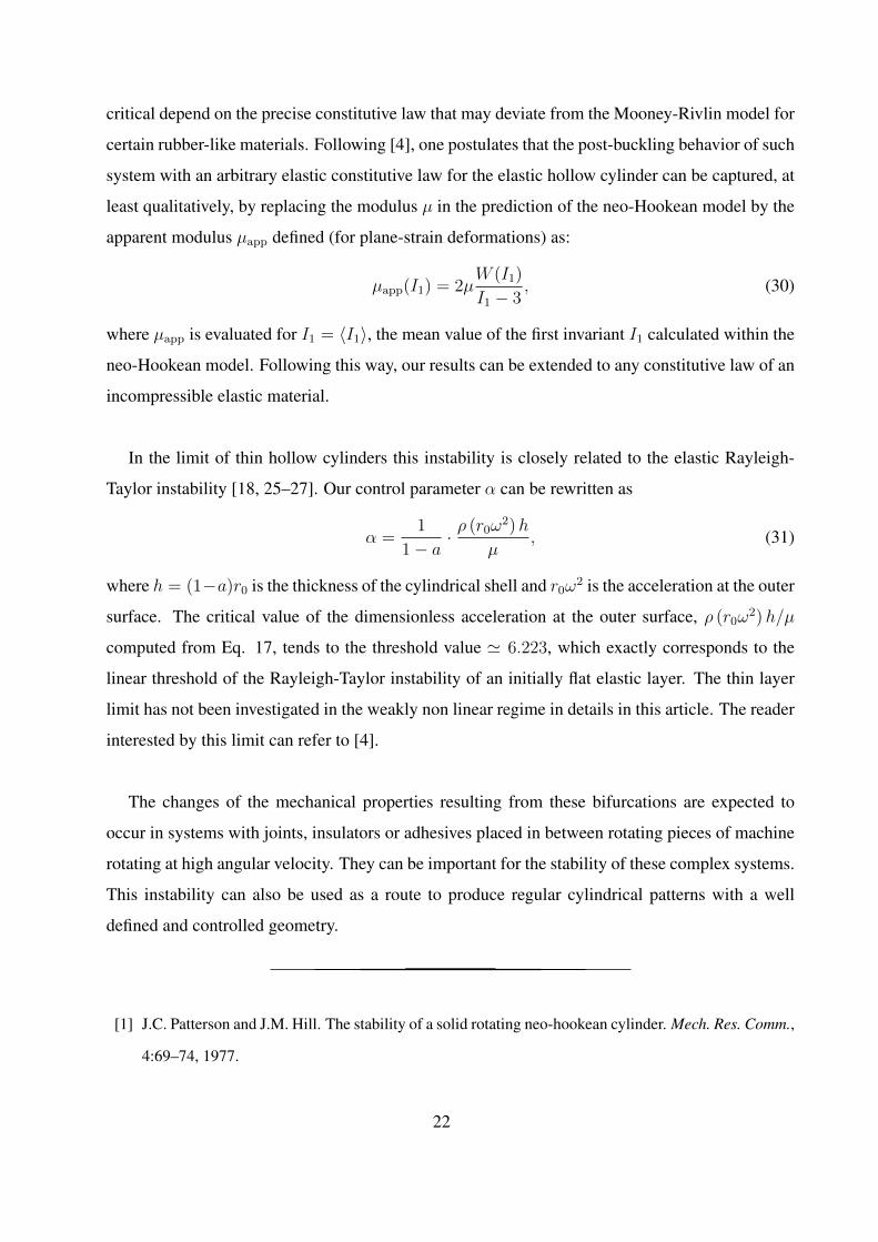
In the limit of thin hollow cylinders this instability is closely related to the elastic Rayleigh-
Taylor instability [18, 25–27]. Our control parameter α can be rewritten as
α =1
1− a ·ρ (r0ω
2)h
µ, (31)
where h = (1−a)r0 is the thickness of the cylindrical shell and r0ω2 is the acceleration at the outer
surface. The critical value of the dimensionless acceleration at the outer surface, ρ (r0ω2)h/µ
computed from Eq. 17, tends to the threshold value ' 6.223, which exactly corresponds to the
linear threshold of the Rayleigh-Taylor instability of an initially flat elastic layer. The thin layer
limit has not been investigated in the weakly non linear regime in details in this article. The reader
interested by this limit can refer to [4].
The changes of the mechanical properties resulting from these bifurcations are expected to
occur in systems with joints, insulators or adhesives placed in between rotating pieces of machine
rotating at high angular velocity. They can be important for the stability of these complex systems.
This instability can also be used as a route to produce regular cylindrical patterns with a well
defined and controlled geometry.
[1] J.C. Patterson and J.M. Hill. The stability of a solid rotating neo-hookean cylinder. Mech. Res. Comm.,
4:69–74, 1977.
22
[2] D.M. Haughton and R.W. Ogden. Bifurcation of finitely deformed rotating elastic cylinders. Q. J.
Mech. appl. Math., 33:251–265, 1980.
[3] P.J. Rabier and J.T. Oden. Bifurcation in rotating bodies. Masson Springer-Verlag, Paris, 1989.
[4] F. Richard, A. Chakrabarti, B. Audoly, Y. Pomeau, and S. Mora. Buckling of a spinning elastic
cylinder: linear, weakly nonlinear and post-buckling analyses. Proc. Roy. soc. A, 474:20180242,
2018.
[5] J. Padovan and O. Paramodilok. Generalized solution of time dependent traveling load problem via
moving finite element scheme. Journal of Sound and Vibration, 91:195–209, 1983.
[6] J.T. Oden and T.L. Lin. On the general rolling contact problem for finite deformations of a viscoelastic
cylinder. Computer Methods in Applied Mechanics and Engineering, 57:297–367, 1986.
[7] A. Chatterjee, J.P. Cusumano, and J.D. Zolock. On contact-induced standing waves in rotating tires:
Experiment and theory. Journal of Sound and Vibration, 227:1049–1081, 1999.
[8] V.V. Krylov and O. Gilbert. On the theory of standing waves in tyres at high vehicle speeds. Journal
of Sound and Vibration, 329:4398–4408, 2010.
[9] S. Govindjee, T. Potter, and J. Wilkening. Dynamic stability of spinning viscoelastic cylinders at finite
deformation. International Journal of Solids and Structures, 51:3589–3603, 2014.
[10] Le Tallec P. and C. Rahler. Numerical models of steady rolling for nonlinear viscoelastic structures in
finite deformations. Int. J. for Numerical Methods in Eng., 37:1159–1186, 1994.
[11] R. Gateaux. Fonctions d’une infinite de variables independantes. Bulletin de la Societe Mathematique
de France, 47:70–96, 1919.
[12] W. T. Koiter. On the Stability of an Elastic Equilibrium. PhD thesis, Delft; H. J. Paris, Amsterdam,
The Netherlands, 1945.
[13] J. W. Hutchinson. Imperfection sensitivity of externally pressurized spherical shells. Journal of Ap-
plied Mechanics, 34:49–55, 1967.
[14] J. W. Hutchinson and W.T. Koiter. Postbuckling theory. Applied Mechanics Reviews, pages 1353–
1366, 1970.
[15] B. Budiansky. Theory of buckling and post-buckling behavior of elastic structures. Advances in
applied mechanics, 14:1–65, 1974.
[16] R. Peek and N. Triantafyllidis. Worst shapes of imperfections for space trusses with many simultane-
ously buckling members. International Journal of Solids and Structures, 29:2385–2402, 1992.
[17] R. Peek and M. Kheyrkhahan. Postbuckling behavior and imperfection sensitivity of elastic structures
23

by the Lyapunov-Schmidt-Koiter approach. Computer methods in applied mechanics and engineering,
108(3):261–279, 1993.
[18] A. Chakrabarti, S. Mora, F. Richard, T. Phou, J.-M. Fromental, Y. Pomeau, and B. Audoly. Selection
of hexagonal buckling patterns by the elastic Rayleigh-Taylor instability. Journal of the Mechanics
and Physics of Solids, 121:234–257, 2018.
[19] A. van der Heijden. W. T. Koiter’s elastic stability of solids and structures. Cambridge University
Press Cambridge, 2009.
[20] Nicolas Triantafyllidis. Stability of solids: from structures to materials. Ecole Polytechnique, 2011.
[21] M. Destrade, M.D. Gilchrist, and J.G. Murphy. Onset of non-linearity in the elastic bending of blocks.
ASME Journal of Applied Mechanics, 77:061015, 2010.
[22] A. Logg, K.A. Mardal, and G. Wells. Automated Solution of Differential Equations by the Finite
Element Method. Springer, 2012.
[23] C. Normand, Y. Pomeau, and M. G. Velarde. Convective instability: a physicist’s approach. Reviews
of Modern Physics, 49(3):581, 1977.
[24] S. Strogatz. Non-linear Dynamics and Chaos: With applications to Physics, Biology, Chemistry and
Engineering. Addison-Wesley, 1994.
[25] S. Mora, T. Phou, J. M. Fromental, and Y. Pomeau. Gravity driven instability in solid elastic layers.
Phys. Rev. Lett., 113:178301, 2014.
[26] X. Liang and S. Cai. Gravity induced crease-to-wrinkle transition in soft materials. Appl. Phys. Lett.,
106:041907, 2015.
[27] D. Riccobelli and P. Ciarletta. Rayleigh-taylor instability in soft elastic layers. Phil. Trans. R. soc. A,
375:20160421, 2017.
[28] See supplementary material.
Appendix A: Linear analysis for prismatic deformations
In this appendix, the main steps leading to the expression of the linear instability threshold
(Eqs.17 and 18) are introduced. Then, the complete expression of the first order displacement is
given.
The fourth order linear equation Eq.14, with the zero traction condition at the lateral boundary,
24
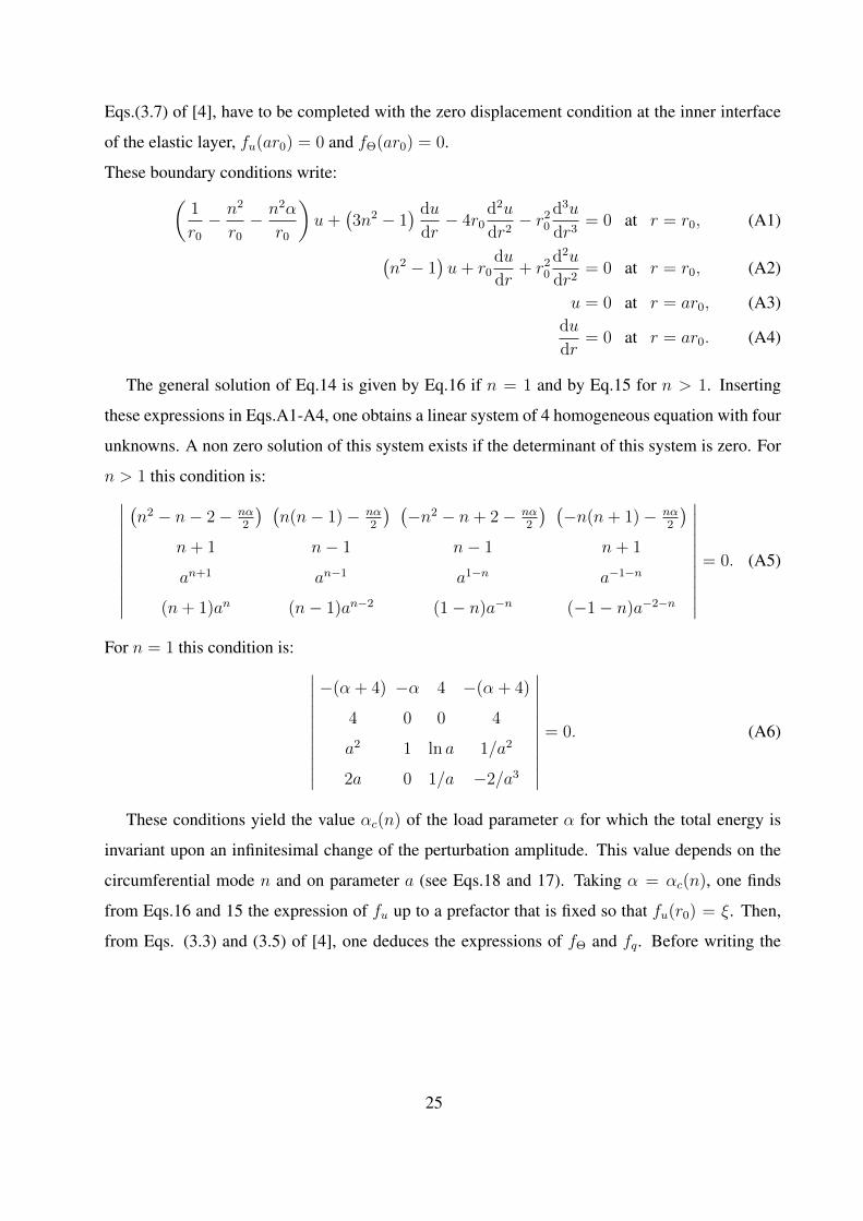
Eqs.(3.7) of [4], have to be completed with the zero displacement condition at the inner interface
of the elastic layer, fu(ar0) = 0 and fΘ(ar0) = 0.
These boundary conditions write:(
1
r0
− n2
r0
− n2α
r0
)u+
(3n2 − 1
) du
dr− 4r0
d2u
dr2− r2
0
d3u
dr3= 0 at r = r0, (A1)
(n2 − 1
)u+ r0
du
dr+ r2
0
d2u
dr2= 0 at r = r0, (A2)
u = 0 at r = ar0, (A3)du
dr= 0 at r = ar0. (A4)
The general solution of Eq.14 is given by Eq.16 if n = 1 and by Eq.15 for n > 1. Inserting
these expressions in Eqs.A1-A4, one obtains a linear system of 4 homogeneous equation with four
unknowns. A non zero solution of this system exists if the determinant of this system is zero. For
n > 1 this condition is:∣∣∣∣∣∣∣∣∣∣∣
(n2 − n− 2− nα
2
) (n(n− 1)− nα
2
) (−n2 − n+ 2− nα
2
) (−n(n+ 1)− nα
2
)
n+ 1 n− 1 n− 1 n+ 1
an+1 an−1 a1−n a−1−n
(n+ 1)an (n− 1)an−2 (1− n)a−n (−1− n)a−2−n
∣∣∣∣∣∣∣∣∣∣∣
= 0. (A5)
For n = 1 this condition is:∣∣∣∣∣∣∣∣∣∣∣
−(α + 4) −α 4 −(α + 4)
4 0 0 4
a2 1 ln a 1/a2
2a 0 1/a −2/a3
∣∣∣∣∣∣∣∣∣∣∣
= 0. (A6)
These conditions yield the value αc(n) of the load parameter α for which the total energy is
invariant upon an infinitesimal change of the perturbation amplitude. This value depends on the
circumferential mode n and on parameter a (see Eqs.18 and 17). Taking α = αc(n), one finds
from Eqs.16 and 15 the expression of fu up to a prefactor that is fixed so that fu(r0) = ξ. Then,
from Eqs. (3.3) and (3.5) of [4], one deduces the expressions of fΘ and fq. Before writing the
25
analytic expressions of fu, fΘ and fq, we first define four constants:
A = −a2n (a2 − 1)n2 + (a2n + a2)n− a2n+2 − a2
a2n (2a4 − 2)n− 2a4n+2 + 2a2,
B =a2n (a4 − a2)n2 + (a2n+4 + a2)n+ a2n+2 + a2
a2n (2a4 − 2)n− 2a4n+2 + 2a2,
C =a2n (a2 − 1)n2 + (−a4n+2 − a2n)n− a4n+2 − a2n+2
a2n (2a4 − 2)n− 2a4n+2 + 2a2,
D = −a2n (a4 − a2)n2 + (−a4n+2 − a2n+4)n+ a4n+2 + a2n+2
a2n (2a4 − 2)n− 2a4n+2 + 2a2. (A7)
The expressions of fu, fΘ and fq are:
fu =
[A
(r
r0
)n+1
+B
(r
r0
)n−1
+ C
(r
r0
)1−n+D
(r
r0
)−n−1]ξ, (A8)
fΘ = −[An+ 2
n
(r
r0
)n+B
(r
r0
)n−2
+ C2− nn
(r
r0
)−n−D
(r
r0
)−n−2]ξ
r0
, (A9)
fq =
[(−4A(n2 + n)− αcB
)( r
r0
)n+(4C(n− n2)− αcD
)( r
r0
)−n
−αcA(r
r0
)n+2
− αcC(r
r0
)2−n]
ξ
r0n2, (A10)
with α = αc(n) (given by Eq.17). The previous expressions are for n > 1. For n = 1, we define:
A =a2
(2 + 2a4) ln a− a4 + 1, (A11)
B = 1, (A12)
C = − 2 + 2a4
(2 + 2a4) ln a− a4 + 1, (A13)
D = − a2
(2 + 2a4) ln a− a4 + 1, (A14)
fu =
[(r0
r
)2
D + ln
(r
r0
)C +B +
(r
r0
)2
A
]ξ, (A15)
fΘ =
[(r0
r
)3
D −(r0
r
)(1 + ln
(r
r0
))C −
(r0
r
)B − 3
(r
r0
)A
]ξ
r0
, (A16)
fq =
[−(
8r
r0
+ αc
(r
r0
)3)A+ αc
r
r0
B +
(αcr
r0
ln
(r
r0
)− 2
r0
r
)C + αc
r0
rD
]ξ
r0
.(A17)
If one considers the limit a → 0 with the circumferential wave number n = 1, one obtains
(A,B,C,D) → (0, 1, 0, 0) hence fu = ξ. Since fu(ar0) = 0, the amplitude ξ of the mode with
n = 1 is fixed to 0 (for a→ 0, [4]).
26
Appendix B: Linear analysis including axial deformations
The main steps for the linear analysis introduced in Sec. III are detailed in this section.
We start from the sixth order differential equation, Eq.11, that was established previously in
[4] in which the bifurcations in homogeneous spinning (solid) cylinders were investigated. The
condition of zero traction at the lateral boundary (r = r0) leads to three equations that were
expressed in terms of fu in [4], see Eqs. (A8) (A9) (A10) of [4]. The zero displacement condition
at the inner interface of the elastic layer leads to three other boundary conditions, fu(ar0) = 0,
fΘ(ar0) = 0 and fz(ar0) = 0, that write, in terms of fu (for r = ar0):
fu = 0, (B1)dfudr
= 0, (B2)
r3 d5fudr5
+ 7r2 d4fudr4
+ r[(
5− 2n2)− 2 (kr)2] d3fu
dr3− 6
[1 + 2 (kr)2] d2fu
dr2= 0. (B3)
In the following we calculate the general solution for Eq.11 for a given circumferential wave
number n. This solution is defined up to 6 arbitrary constants. The solvability condition is fixed
by the six boundary equations, and leads to a relation between α and a, defining the critical load
αc(n, k) at the linear instability threshold.
Although the physically admissible values of r are in the range [ar0, r0], one can consider the
mathematical solutions of Eq.11 in a the wider range of values of r, here in [0, r0]. In order to find
linearly independent solutions of Eq.11, we consider the mathematical behaviour of the solutions
of this sixth order linear differential equation in the limit r → 0. Let us first assume that fu(r) ∼ rp
as r → 0. Substituting this particular expression of fu in Eq.11 and considering the limit r → 0,
the condition on exponent p is:
(n+ p− 3)(n− p− 1)(n− p+ 1)(n− p+ 3)(n+ p− 1)(n+ p+ 1) = 0. (B4)
In the following, the linear solvability condition is derived for axisymmetric modes (circumfer-
ential wave number n = 0, Sec. B 1), and mixed modes with n = 1 (Sec. B 2), n = 2 (Sec. B 3)
and n = 3 (Sec. B 4).
27
1. Axisymmetric modes
Here, we consider the deformations that are invariant by a continuous rotation about the axis of
the cylinder, i.e. n = 0. The roots of Eq.B4, p = −1, 1 and 3 are double. We search accordingly
six independent solutions of Eq.11, named s1(r), s2(r), s3(r), s4(r), s5(r) and s6(r) so that, for
r → 0, s1(r) ∼ 1/r, s2(r) ∼ r, s3(r) ∼ r3, s4(r) ∼ ln r/r, s5(r) ∼ r ln r and s6(r) ∼ r3 ln r.
The general expression of the solutions of Eq.11 are therefore sought as:
si(r) =a−1
kr+b−1 ln(kr)
kr+∞∑
m=0
(am + bm ln(kr)) (kr)m. (B5)
The substitution of this expression in Eq.11 yields the conditions on the sequences (am)m≥−1 and
(bm)m≥−1:
b−1 − 12b1 + 192b3 − 2304b5 = 0, (B6)
a−1 − 12a1 + 192a3 − 2304a5 − 12b1 + 288b3 − 4224b5 = 0, (B7)
bm−6−3(m−3)2bm−4+3(m−3)2(m−1)2bm−2−(m−3)2(m−1)2(m+1)2bm = 0 ∀m ≥ 6 (B8)
am−6 − 3(m− 3)2am−4 + 3(m− 3)2(m− 1)2am−2 − (m− 3)2(m2 − 1)2am
−6(m− 3)bm−4 + 12(m− 1)(m− 2)(m− 3)bn−2 + 2(m− 3)(m2 − 1)(1 + 6m− 3m2)bm = 0
∀m ≥ 6.
Moreover, am and bm are equal to 0 if n is an even number. Eqs.B6 and B7 involve 8 unknowns
(a−1, a1, a3, a5, b−1, b1, b3, b5), leaving 6 free unknown that are chosen accordingly with the
prescribed behaviour of the functions si for r → 0, leading to the following sequences:
a−1 = 1, a1 = a3 = 0, b−1 = b1 = b3 = 0 for s1(r),
a−1 = 0, a1 = 1, a3 = 0, b−1 = b1 = b3 = 0 for s2(r),
a−1 = a1 = 0, a3 = 1, b−1 = b1 = b3 = 0 for s3(r),
a−1 = 1, a1 = a3 = 0, b−1 = 1, b1 = b3 = 0 for s4(r),
a−1 = 0, a1 = 1, a3 = 0, b−1 = 0, b1 = 1, b3 = 0 for s5(r),
a−1 = a1 = 0, a3 = 1, b−1 = b1 = 0, b3 = 1 for s6(r).
Writing fu(r) as:
fu(r) =6∑
i=1
Aisi(r), (B9)
and substituting this expression of fu(r) in the boundary equations, one obtains a homogeneous
linear system of 6 equations with 6 unknowns. The solvability condition implies that the matrix
28

of the system is singular, hence the equation defining the threshold value of αc as a function of k
that is solved numerically and plotted in Fig.3.
2. Asymmetric mode with the circumferential wave number n = 1
We now focus on mixed modes with the circumferential wave number n = 1. The roots of
Eq.B4 are p = −2, 0, 2, 4 (2 and 0 are double roots). Then we search six independent solutions of
Eq.11 so that, for r → 0, s1(r) ∼ 1/r2, s2 ∼ 1, s3(r) ∼ ln r, s4(r) ∼ r2, s5 ∼ r2 ln r, s6 ∼ r4, in
the form of the series expansion:
si(r) =a−2
r2+∞∑
m=0
(am + bm ln(kr)) (kr)m. (B10)
The substitution of this expression in Eq.11 yields the condition on the sequences (am)m≥−2 and
(bm)m≥0:
a−2 − 6b0 + 48b2 − 384b4 = 0, (B11)
bm−6 − 3(m− 4)(m− 2)bm−4 + 3(m− 4)(m− 2)2mbm−2 − (m− 4)(m− 2)2m2(2 +m)bm = 0 ∀m ≥ 6,
(B12)
am−6 − 3(m− 4)(m− 2)am−4 + 3(m− 4)(m− 2)2mam−2
−(m− 4)(m− 2)2m2(m+ 2)am − 6(m− 3)bm−4 + 12(m− 2)(m2 − 4m+ 2)bm−2
−2(m− 2)(m− 1)m(−16− 6m+ 3m2)bm = 0 ∀m ≥ 6.
(B13)
Moreover, am and bm are equal to 0 for n odd number. Accordingly with the prescribed behaviour
of the functions si for r → 0, we take the following sequences :
a−2 = 1, a0 = a2 = a4 = b0 = b2 = 0 for s1(r),
a−2 = 0, a0 = 1, a2 = a4 = b0 = b2 = 0 for s2(r),
a−2 = a0 = a2 = a4 = 0, b0 = 1, b2 = 0 for s3(r),
a−2 = a0 = 0, a2 = 1, a4 = b0 = b2 = 0 for s4(r),
a−2 = a0 = a2 = a4 = b0 = 0, b2 = 1 for s5(r),
a−2 = a0 = a2 = 0, a4 = 1, b0 = b2 = 0 for s6(r).
Following the same procedure as in Sec. B 1, one then obtains the threshold value αc as a function
of k for n = 1 (See Fig.3).
29
3. Asymmetric mode with the circumferential wave number n = 2
We now deal with mixed modes with the circumferential wave number n = 2. The roots of
Eq.B4 are p = −3,−1, 1 (double root), 3 and 5. Then we search six independent solutions of
Eq.11 so that, for r → 0, s1(r) ∼ 1/r3, s2(r) ∼ 1/r, s3(r) ∼ r, s4 ∼ r ln r, s5 ∼ r3 and s6 ∼ r5,
in the form of the series expansion:
si(r) =a−3
(kr)3+a−1
kr+∞∑
m=0
(am + bm ln(kr)) (kr)m. (B14)
The substitution of this expression in Eq.11 yields the condition on the sequences (am)m≥−3 and
(bm)m≥0:
−48b1 + 192b3 + 12a−1 + a−3 = 0, (B15)
−12b1 + 144b3 − 1536b5 + a−1 = 0, (B16)
bm−6 − 3(m− 5)(m− 1)bm−4 + 3(m− 5)(m− 3)(m2 − 1)bm−2
−bm(m− 5)(m2 − 9)(m− 1)2(m+ 1) = 0 ∀m ≥ 6,(B17)
am−6 − 3(m− 5)(m− 1)am−4 + 3(m− 5)(m− 3)(m2 − 1)am−2
−(m− 5)(m2 − 9)(m− 1)2(m+ 1)an
−6(m− 3)bm−4 + 12(m− 2)(m2 − 4m− 1)bm−2
−2(m− 1)(27 + 68m− 22m2 − 12m3 + 3m4)bm = 0 ∀n ≥ 6.
(B18)
Moreover, am and bm are equal to 0 for n even number. Accordingly with the prescribed behaviour
of the functions si for r → 0, we take the following sequences :
a−3 = 1, a−1 = a1 = a3 = a5 = b1 = 0 for s1(r),
a−3 = 0, a−1 = 1, a1 = a3 = a5 = 0 = b1 = 0 for s2(r),
a−3 = 0 = a−1 = 0, a1 = 1, a3 = a5 = b1 = 0 for s3(r),
a−3 = a−1 = a1 = a3 = a5 = 0, b1 = 1 for s4(r),
a−3 = a−1 = a1 = 0, a3 = 1, a5 = b1 = 0 for s5(r),
a−3 = a−1 = a1 = a3 = 0, a5 = 1, b1 = 0 for s6(r).
Following the same procedure as in Sec. B 1, one then obtains the threshold value αc as a function
of k for n = 2 (See Fig.3).
30

4. Asymmetric mode with the circumferential wave number n = 3
For n = 3, the roots of Eq.B4 are p = −4,−2, 0, 2, 4 and 6. Then, we take s1(r) ∼ 1/r4,
s2(r) ∼ 1/r2, s3(r) ∼ 1, s4 ∼ r2, s5 ∼ r4 and s6 ∼ r6 for r → 0. Function si(r) are sought as:
si(r) =a−4
(kr)4+
a−2
(kr)2+∞∑
m=0
(am + bm ln(kr)) (kr)m, (B19)
leading to the conditions:
24a0 − 144b2 + 768b4 + a−2 = 0, (B20)
192a0 − 384b2 + 24a−2 + a−4 = 0, (B21)
bm−6 − 3(m− 6)mbm−4 + 3(m− 6)(m− 4)m(m+ 2)bm−2
−(m− 6)(m− 4)(m− 2)m(m+ 2)(m+ 4)bm = 0 ∀m ≥ 6,(B22)
am−6 − 3(m− 6)mam−4 + 3(m− 6)(m− 4)m(m+ 2)am−2
−(m− 6)(m2 − 16)(m2 − 4)mam
−6(m− 3)bm−4 + 12(m− 2)(m2 − 4m− 6)bm−2
−2(m− 1)(192 + 128m− 52m2 − 12m3 + 3m4)bm = 0 ∀m ≥ 6.
(B23)
Moreover, am and bm are equal to 0 for n even number. Accordingly with the prescribed behaviour
of the functions si for r → 0, we take the following sequences :
a0 = 1, a2 = a4 = a6 = b2 = b4 = 0 for s1(r),
a−4 = 0, a−2 = 1, b4 = a2 = a4 = a6 = 0 for s2(r),
a−4 = a−2 = 0, a0 = 1, a2 = a4 = a6 = 0 for s3(r),
a−4 = a−2 = a0 = 0, a2 = 1, a4 = a6 = 0 for s4(r),
a−4 = a−2 = a0 = 0 = a2 = 1, a4 = 1, a6 = 0 for s5(r),
a−4 = a−2 = a0 = a2 = a4 = 0, a6 = 1 for s6(r).
Following the same procedure as in Sec. B 1, one then obtains the threshold value αc as a function
of k for n = 3 (See Fig.3).
The same analyze, done for circumferential wave numbers n ≥ 4, qualitatively leads to the
same structure for αc(n, k).
31

Appendix C: Calculation of the displacement field at order 2 in the weakly non linear analysis
The key steps in the calculation of the second order solution in the post buckling expansion are
introduced in this appendix.
For the neo-Hookean constitutive law we consider, the strain energy density function is W =
12
(I1 − 3). The strong form of the equilibrium condition Eq.5 is deduced from Eqs. (2.5)-(2.9) of
[4]. It is:
R
r(R,rΘ,θ −R,θΘ,r) = 1, (C1)
− (rR,r),r −R,θθ
r+ rR (Θ,r)
2 +R
r(Θ,θ)
2 −Rq,rΘ,θ +Rq,θΘ,r = αrR
r20
, (C2)
(rR2Θ,r
),r
+1
r
(R2Θ,θ
),θ
+Rq,θR,r −Rq,rR,θ = 0, (C3)
rR,r + qRΘ,θ = 0 at r = r0, (C4)
rRΘ,r − qRθ = 0 at r = r0, (C5)
R = r at r = ar0, (C6)
Θ = θ at r = ar0, (C7)
where a subscript comma denotes a partial derivative. Eq.C1 is the incompressibility constraint,
Eqs.C2 and C3 are the equilibrium conditions in the radial and circumferential directions respec-
tively, Eqs.C4 and C5 are the zero traction condition at the lateral boundary r = r0, and Eqs.C6
and C7 are the zero displacement condition at the rigid inner rod.
The expansions defined in Eqs.19 and 20 are first put in Eqs.C1-C7:
α = αc + ε2α2,
R = r + εu1 + ε2u2,
Θ = θ + εΘ1 + ε2Θ2,
q = q0 + εq1 + ε2q2.
q0, as defined by Eq.9, contains known contributions at order ε0 and at order ε2. u1, Θ1 and q1
have been calculated up to the amplitude ξ in the linear analysis (Appendix A). u2, Θ2 and q2 are
defined by Eqs.25-27 through the unknown functions gu, gΘ, gq, gu, gΘ and gq. The goal is here to
find the expressions of these 6 functions for given a, n, α2 and ξ.
32

Eqs.C1-C7 at order ε2 yield a set of 7 equations. Each one can be separated in two parts :
one is independent of θ and involves gu, gΘ and gq. The other part depends on θ like cos(4nθ) or
sin(4nθ) and involves gu, gΘ and gq. At the end, one obtains 14 differential equations:
• 3 coupled linear differential equations in the bulk for gu, gq and gΘ with 4 boundary condi-
tions (at r = r0 and r = ar0);
• 3 coupled linear differential equations in the bulk for gu, gq and gΘ with 4 boundary condi-
tions (at r = r0 and r = ar0);
Combining the θ dependent terms of order ε2 arising from Eqs.C2, C3 and C1, one obtains a
fourth order linear differential equation for gu:
r3 d4gudr4
+ 6r2 d3gudr3− (8n2 − 5)r
d2gudr2− (8n2 + 1)
dgudr
+ (4n2 − 1)2 gur
= −(ξ
r0
)2
h1, (C8)
where h1 is a function of r/r0, n and a. The complete expression of h1 is given in [28]. The
solutions of Eq.C8 can be written as:
gu(r) = A2r−(2n+1) +B2r
−(2n−1) + C2r2n−1 +D2r
2n+1 +
(ξ
r0
)2
γ(r), (C9)
with
γ(r) = lnr
r0
(k0r
r0
+ k1r0
r+ k2
(r0
r
)3
+ k4r0
rlnr
r0
)+ k3
(r0
r
)5
for n = 1,
γ(r) = k0r/r0 + k1(r/r0)2n−3 +k2
(r/r0)3+ k3(r/r0)−(2n+3) +
k4
(r/r0)for n > 1.
(C10)
A2, B2, C2 and D2 are four constants and k0, k1, k2, k3 and k4 depend on a and n. Their complete
expressions are written in [28]. From Eqs.C4, C5, C1, and C3 at order ε2, one obtains the boundary
conditions at r = r0 expressed in terms of gu:
r30
d3gudr3
(r0) + 4r20
d2gudr2
(r0)− (12n2 − 1)r0dgudr
(r0) + h2gu(r0) = −ξ2
r0
h3, (C11)
r20
d2gudr2
(r0) + r0dgudr
(r0) + (4n2 − 1)gu(r0) = − ξ2
2r0
h4. (C12)
h2, h3 and h4 are three functions of a and n, whose detailed expressions are given in [28]. The two
remaining boundary conditions to be taken into account in order to determine the constants A, B,
C and D in Eq.C9 are:
gu(ar0) = 0, (C13)
gΘ(ar0) = 0. (C14)
33
Eq.C14 is expressed with gΘ which can be written in terms of gu using Eq.C1.
Inserting Eq.C10 in the four boundary equations, Eqs.C11-C14, one obtains a system of four
equations with four unknowns, A2, B2, C2 and D2, that are determined as a function of a and n,
hence the complete analytical expression for gu(r).
gΘ and gq are obtained from Eqs.C1 and C3 respectively, by inserting in these equations the
previous expression of gu.
Taking now the terms independent of θ in the second order term of Eq.C1, one obtains a first
order differential equation for gu:
rdgudr
+ gu =r2
0ξ2
r3h7, (C15)
with h7 a function of a, n and r/r0 whose expression is given in [28]. This first order linear
differential equation can be solved using the variation of parameters method up to a constant,
which is fixed with the θ-independent part of boundary condition Eq.C6 at order ε2:
gu(ar0) = 0. (C16)
The expression of gu being now known, the first derivative of qq, dqq/dr, can be calculated
from the θ-independent part of Eq.C2 at order ε2 which is:
rd2gudr2
+dgudr
+ rdgqdr− gu
r= −ξ
2
r20
h5. (C17)
h5 is a function of a, n and r/r0 whose expression is given in [28]. The expression of gq is obtained
by integration of dqq/dr with the boundary condition Eq.C4 which is:
r0dgudr
(r0)− gu (r0) + r0gq (r0) = −h6, (C18)
where h6 is a function of a and n, whose expression is given in [28].
The θ-independent part of Eq.C3 yields the first order linear homogeneous differential equation
for dqΘ/dr:
r3 d2gΘ
dr2+ 3r2 dgΘ
dr= 0. (C19)
With C5 and C6, which write respectively at order ε2:
dgΘ
dr(r0) = 0, (C20)
34

and
gΘ(ar0) = 0, (C21)
one deduces that gΘ = 0.
Appendix D: List of symbols assigned to specific load parameters and relative inner radii
The symbols defining special values of the load parameter α and special values of the relative
inner radius a used in Sections III, IV and V are summarized below. n is the order of the rotational
symmetry of the buckled configuration, and nfirst is the value of n of the first mode that is linearly
unstable when α is gradually increased from 0. nfirst depends on a.
Symbol Description
alinearn value of a at the crossover from nfirst = n− 1 to nfirst = n
a−n lowest value of a so that mode n is sub-critical
a+n lowest value of a for a crossover from sub-critical to super-critical (for fixed
mode n)αc(n) critical load at the linear instability threshold. αc(n) also depends on a
α∗(nmesh) critical load at the linear instability threshold calculated with finite elements
with the linear mesh density nmesh. α∗(nmesh) also depends on a and nαm(n) lowest admissible load for a buckled configuration with a rotational symmetry
of order n. αm(n) also depends on aαm lowest admissible load for a buckled configuration, whatever the rotational
order. αm depends on a
35