Embed Size (px)
Citation preview

Brixen Workshop and Summer School on InternationalTrade and Finance
Part 4: Quasi-Experimental Geography
Daniel Sturm
London School of Economics
1

Brixen Workshop 2012 - 2 - Daniel Sturm
1 Introduction
• This part of the workshop starts from the old question whatdetermines the spatial distribution of economic activity.
• Economic activity is highly unevenly distributed across countriesand also across regions within countries.
• A key question is what causes these differences in the level ofeconomic activity.
•We will focus mainly on the distribution of economic activityacross regions or cities within countries.

Brixen Workshop 2012 - 3 - Daniel Sturm
• There are at least two broad explanations for the unequaldistribution of empirical activity across space within countries:
– Fundamentals: differences in the fundamental productivity oflocations.
– Agglomeration Forces: Proximity to other economic agentsincreases the attractiveness of a location.
• These two mechanisms are obviously not exclusive and can bothoperate at the same time.
• The key empirical question is to what extent observed patterns ofactivity are explained by these two mechanism.

Brixen Workshop 2012 - 4 - Daniel Sturm
•Whether fundamentals or agglomeration forces are responsible forthe pattern of economic activity has important implications for thepersistence of spatial equilibria.
• Suppose for example that only agglomeration forces are operating.
• In this case the location of economic activity is rather arbitrary - alocation is attractive because other workers are locating there.
• This is a bit like choosing a nightclub: club A is “cool” because allthe “cool” people go to club A rather than club B.
• If instead only fundamentals are operating then the distribution ofactivity is determined by the distribution of fundamentals.

Brixen Workshop 2012 - 5 - Daniel Sturm
• If agglomeration forces rather than fundamentals dominate thespatial distribution of activity this also has key policy implications.
• In this case regional policy could try to move the distribution ofactivity between different equilibria.
•With a temporary subsidy regions could try to attract a “criticalmass” of economic activity.
• Once this critical mass has been established, the location remainsattractive even when the subsidy has ended.

Brixen Workshop 2012 - 6 - Daniel Sturm
1.1 Overview
• The theoretical roots of economic geography
• Fundamentals versus agglomeration forces
• Empirical evidence: Bombing
• Empirical evidence: German division
• Empirical evidence: Portage
• Outlook for future research

Brixen Workshop 2012 - 7 - Daniel Sturm
2 The Origins of Economic Geography
• Krugman (1979) started the new trade theory.
• This paper already contains almost all the ideas necessary for thenew economic geography model of Krugman (1991).
•We will briefly review the key building blocks of Krugman (1979)before looking at what economic geography has added to thismodel.

Brixen Workshop 2012 - 8 - Daniel Sturm
2.1 Basic Assumptions of Krugman (1979)
• There are two countries.
• Labor is the only factor of production. Endowments L and L∗.
•Many firms, which produce differentiated products i ∈ [1, n] .
• Preferences are:
U =n∑i=1
v(ci) (1)
with v′ > 0 and v′′ < 0. These preferences incorporate “love ofvariety”.

Brixen Workshop 2012 - 9 - Daniel Sturm
• Technology is:li = α + βxi (2)
with α, β > 0.
• Note that this production function has increasing returns to scale.
• Firms are monopolistically competitive, i.e. they ignore the effectsof their decisions on others and set prices like a monopolist.
• For now assume that there is no trade between the two countries.

Brixen Workshop 2012 - 10 - Daniel Sturm
2.2 Equilibrium
• In autarky the equilibrium in each country is a simply trade-off:
– Love of variety means that ceteris paribus consumers want asmuch variety as possible.
– However, increasing returns mean that each new variety requiresthe fixed labor requirement α.
• The number of varieties that a country produces in equilibriumdepends entirely on its labor endowment.
• Key result: the larger country will produce more variety inequilibrium and offer higher real wages.

Brixen Workshop 2012 - 11 - Daniel Sturm
2.3 Allowing Migration
• Krugman points out at the end of his 1979 paper that if migrationis allowed people will want to move from small to large countries.
•We can also interpret “countries” as regions or cities.
• This incentive for people to agglomerate in the large country orregion continues to exist even if we allow trade in goods.
• The migration incentive only disappears if the “world is flat” andthere are zero trade costs.
• You have already learned earlier this week that empirically theearth is anything but flat.

Brixen Workshop 2012 - 12 - Daniel Sturm
3 Fundamentals versus Path Dependence
• The simple Krugman (1979) model with migration can capture thebasic idea of multiple equilibria and path dependence.
• Consider a situation in which initially the two regions have thesame population.
• Now suppose some workers move from region one to region two.
• This shift increases real wages in region two and induces furthermigration into region two.
• This cumulative causation will draw the entire population of regionone into region two.

Brixen Workshop 2012 - 13 - Daniel Sturm
• If instead workers had moved from region two to region one, thenregion one would have ended up with all workers.
• The model therefore predicts that there are multiple equilibria.
•Which region becomes the large region depends on potentiallysmall historical accidents.

Brixen Workshop 2012 - 14 - Daniel Sturm
3.1 The Role of Fundamentals
• In the simple model considered above the two regions are equally“good” locations for workers ex-ante.
• Apart from the number of workers locating in a region there are noother factors that determine the attractiveness of a location.
• An alternative reason why workers locate in a region are differencesin fundamentals that determine the productivity of regions.
• A very basic way of capturing this idea in our framework aredifferences in the marginal labor requirement β between regions.

Brixen Workshop 2012 - 15 - Daniel Sturm
• Suppose for example that β is lower in region one because of afavorable climate or access to navigable waterways.
• If such a difference in productivity is large enough it will eliminatethe possibility of path dependence.
• The more productive region will attract all workers even if atemporary shock has displaced many or all workers to the lessproductive region.

Brixen Workshop 2012 - 16 - Daniel Sturm
3.2 Jargon: First versus Second Nature
• The forces of cumulative causation are in the literature oftenreferred to as “second nature” advantages of a location.
• In contrast differences in the fundamental attractiveness oflocations are referred to as “first nature” advantages of a location.

Brixen Workshop 2012 - 17 - Daniel Sturm
3.3 Jargon: Multiple Equilibria
•Macroeconomists typically reserve the term “multiple equilibria” tomodels where expectations determine which equilibrium is selected.
• Cases in which historical accidents determine which of severalpotential equilibria is selected are called “multiple steady-states”or “path-dependence”.
• Other fields are less religious about this and refer to any situationwhere there are several potential equilibria as “multiple equilibria”.
•We will follow this more relaxed definition of multiple equilibria.

Brixen Workshop 2012 - 18 - Daniel Sturm
3.4 Policy Implications
•Whether location patterns are determined by fundamentals (firstnature) or agglomeration forces (second nature) has importantpolicy implications.
• Governments spend considerable amounts of money trying to shifteconomic activity from one location to another.
• Implicitly, a key rational for such policies is that agglomerationforces and path dependence are important.

Brixen Workshop 2012 - 19 - Daniel Sturm
• The hope is that temporary subsidies can create a “critical mass”of economic activity in a location that makes the locationself-sustaining.
• If instead location patterns are mainly determined by fundamentalstemporary interventions are futile.

Brixen Workshop 2012 - 20 - Daniel Sturm
3.5 The Key Empirical Question
• To what extent is the observed distribution of economic activitydetermined but fundamentals or agglomeration forces and pathdependence?
• This question has generated a lot of discussion over the lastdecades.
• For some proponents of economic geography the answer to thisquestion is almost self-evident (see the quote on the next slide):

Brixen Workshop 2012 - 21 - Daniel Sturm
“[T]he dramatic spatial unevenness of the real economy - thedisparities between densely populated manufacturing belts andthinly populated farm belts, between congested cities anddesolate rural areas; the spectacular concentration of particularindustries in Silicon Valleys and Hollywoods - is surely the resultnot of inherent differences among locations but of some set ofcumulative processes, necessarily involving some form ofincreasing returns, whereby geographic concentration can beself-reinforcing.” (Fujita et al., 1999, p. 2)

Brixen Workshop 2012 - 22 - Daniel Sturm
3.6 Empirical Approaches
•More systematic approaches that try to distinguish betweenfundamentals and agglomeration forces have taken two main forms:
– Evidence on the persistence of spatial equilibria
– Exploiting the impact of temporary shocks
• A number of papers show that the spatial distribution ofpopulation and economic activity is surprisingly persistent.

Brixen Workshop 2012 - 23 - Daniel Sturm
• Davis and Weinstein (2002) report, for example, that for Japan thecorrelation between population densities in 1600 and 1998 is astaggering 0.76 (raw correlation) and 0.83 (rank correlation).
•While such evidence is striking it could in principle be due to:
– Fundamentals are key and fundamentals do not change muchover time.
– There are strong agglomeration forces that lock in locationpatterns once established.
Brixen Workshop 2012 - 24 - Daniel Sturm
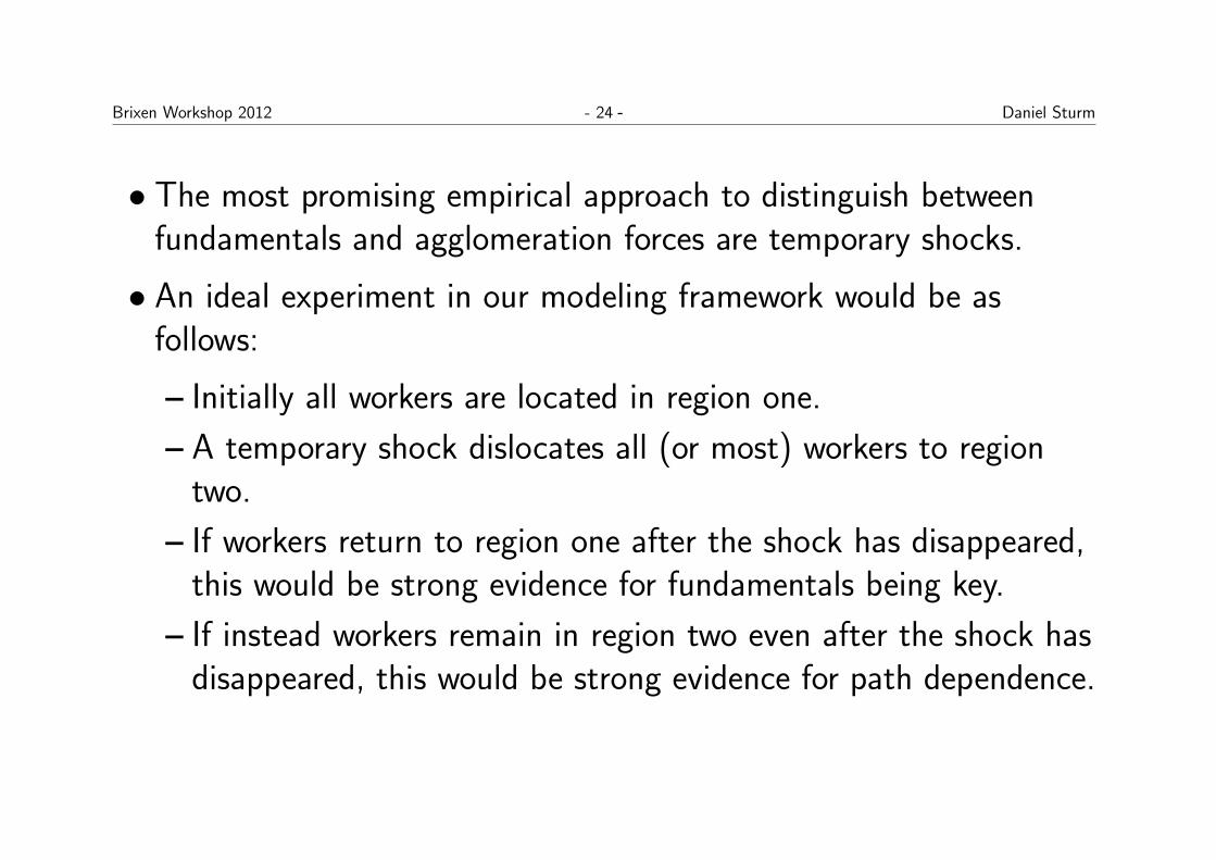
• The most promising empirical approach to distinguish betweenfundamentals and agglomeration forces are temporary shocks.
• An ideal experiment in our modeling framework would be asfollows:
– Initially all workers are located in region one.
– A temporary shock dislocates all (or most) workers to regiontwo.
– If workers return to region one after the shock has disappeared,this would be strong evidence for fundamentals being key.
– If instead workers remain in region two even after the shock hasdisappeared, this would be strong evidence for path dependence.

Brixen Workshop 2012 - 25 - Daniel Sturm
4 Empirical Testing: Bombing
• Davis and Weinstein (2002) were the first to exploit a large scalenatural experiment to distinguish between agglomeration forcesand fundamentals.
• In particular they exploit the Allied bombing of Japanese citiesduring the Second World War as a large but temporary shock.
• Destruction due to bombing was not only large but also veryasymmetric across Japanese cities.

Brixen Workshop 2012 - 26 - Daniel Sturm
• The basic idea behind their approach is to examine whether thepartial destruction of cities during the war had permanent effectson city size.
• If this was the case, this would be powerful evidence for multipleequilibria and path-dependence.

Brixen Workshop 2012 - 27 - Daniel Sturm
4.1 Historical Background
• The bombing of Japan during the Second World War devastatedthe targeted 66 cities, destroying approximately half their housingstock.
• Approximately three hundred thousand Japanese were killed.
• Particularly famous are obviously Hiroshima and Nagasaki due tothe nuclear bombs dropped on them.

Brixen Workshop 2012 - 28 - Daniel Sturm
• However, the majority of cities in the sample suffer essentially nodestruction (and this includes several large cities).
• Despite its scale, the bombing was clearly a temporary shock.
•While it killed many people, destroyed houses and otherinfrastructure it did not change the fundamental attractiveness oflocations.
• A possible exception is the nuclear radiation in Hiroshima andNagasaki, which we will return to.

Brixen Workshop 2012 - 29 - Daniel Sturm
4.2 Data
• Data covers 303 Japanese cities with population in excess of30,000 in 1925.
• The population data is available every 5 years.
• The only exception is the 1945 census which took place in 1947.
• One measure of the intensity of the shocks are the dead or missingcity residents.

Brixen Workshop 2012 - 30 - Daniel Sturm
4.3 Empirical Approach
• Davis and Weinstein (2002) motivate their key regression with asimple statistical model.
• Suppose that the log of the share of city i’s population in totalpopulation at time t is sit and is equal to:
sit = Ωi + εit (3)
where Ωi is the initial size and εit are city specific shocks.
• The persistence of these shocks is modeled as:
εit+1 = ρεit + νit+1 (4)

Brixen Workshop 2012 - 31 - Daniel Sturm
• If ρ ∈ [0, 1] equals one city growth would be a random walk withtemporary shocks having permanent effects.
• If ρ is instead equal to zero temporary shocks only have temporaryeffects on the distribution of population across cities.
• Taking first differences of (3) results in:
sit+1− sit = εit+1− εit (5)
• Now (repeatedly) substituting (4) in (5) results in the finalestimating equation:
sit+1− sit = (ρ− 1)νit + [νit+1 + ρ(ρ− 1)εit−1] (6)

Brixen Workshop 2012 - 32 - Daniel Sturm
• If ρ equals one (6) simplifies to
sit+1− sit = νit+1 (7)
and city population follow a random walk.
• Equation (6) is implemented empirically by regressing:
pgrowth65−47,i = β0 + β1pgrowth47−40,i + ui (8)
where population growth between 1947 and 1940 is the measure ofthe innovation (i.e. war time shock).
• Note that β0 will capture aggregate population growth across allcities and hence changes in shares are equal to growth rates.

Brixen Workshop 2012 - 33 - Daniel Sturm
4.4 Instrumental Variable Strategy
• Note that the measure of innovation in (8) vit will depend on pastshocks to city growth (εit−1).
• To overcome this problem Davis and Weinstein (2002) instrumentfor vit with war-time destruction (deaths and housing stock lost).
• The identifying assumption is that war related destruction wasdetermined by military factors, which are uncorrelated with pre-wargrowth shocks.
• As an additional robustness test the 1925 to 1940 growth rate isincluded as an additional explanatory variable.

Brixen Workshop 2012 - 34 - Daniel Sturm
4.5 Results
• Before estimating (8) we will have a look at a simple scatter plotof city growth rates.
• The following slide contains the key estimation results.

Brixen Workshop 2012 - 35 - Daniel SturmTHE AMERICAN ECONOMIC REVIEW
(5) Sit+1 = Sit + 12it?I*
If p E [0, 1), then city share is stationary and any shock will dissipate over time. In other words, these two hypotheses can be distin- guished by identifying the parameter p.
One approach to investigating the magnitude of p is to search for a unit root. It is well known that unit root tests usually have little power to separate p < 1 from p = 1. This is due to the fact that in traditional unit root tests the inno- vations are not observable and so identify p with very large standard errors. A major advantage of our data set is that we can easily identify the innovations due to bombing. In particular, since by hypothesis the innovation, vit, is uncorre- lated with the error term (in square brackets), then if we can identify the innovation, we can obtain an unbiased estimate of p.
An obvious method of looking at the innova- tion is to use the growth rate from 1940 to 1947. However, this measure of the innovation may contain not only information about the bombing but also past growth rates. This is a measure- ment error problem that could bias our estimates in either direction depending on p. In order to solve this, we instrument the growth rate from 1940-1947 with buildings destroyed per capita and deaths per capita.20
We can obtain a feel for the data by consid- ering the impact of bombing on city growth rates. As we argued earlier, if city growth rates follow a random walk, then all shocks to cities should be permanent. In this case, one should expect to see no relationship between historical shocks and future growth rates. Moreover, if one believes that there is positive serial corre- lation in the data, then one should expect to see a positive correlation between past and future growth rates. By contrast, if one believes that location-specific factors are crucial in under- standing the distribution of population, then one should expect to see a negative relationship between a historical shock and the subsequent growth rate. In Figure 1 we present a plot of
20 The actual estimating equation is Si60 -
Si47 = ( -
1)1V47 + [vi60 + P(P - 1)~i34] Our measure of the innovation is the growth rate between 1940 and 1947 or Si47
- Si40 = ^t47 + [Pi34
- 8i40]. This is clearly
correlated with the error term in the estimating equation, hence we instrument.
1.0-
r- I'*
0.- cr
0
0 2 0
oooo
0o ? 0o(~ 0 0 (^& Q^&(
Oo o
o
-0.5 0 0.5 Growth Rate 1940-1947
FIGURE 1. EFFECTS OF BOMBING ON CITIES WITH
MORE THAN 30,000 INHABITANTS
Note: The figure presents data for cities with positive casu-
alty rates only.
population growth between 1947 and 1960 with that between 1940 and 1947. The sizes of the circles represent the population of the city in 1925. The figure reveals a very clear negative relationship between the two growth rates. This indicates that cities that suffered the largest population declines due to bombing tended to have the fastest postwar growth rates, while cities whose populations boomed conversely had much lower growth rates thereafter.
In Table 2, we present a regression showing the power of our instruments. Deaths per capita and destruction per capita explain about 41 per- cent of the variance in population growth of cities between 1940 and 1947. Interestingly, although both have the expected signs, destruc- tion seems to have had a more pronounced effect on the populations of cities. Presumably, this is because, with a few notable exceptions, the number of people killed was only a few percent of the city's population.
We now turn to test whether the temporary shocks give rise to permanent effects. In order to estimate equation (4), we regress the growth rate of cities between 1947 and 1960 on the growth rate between 1940 and 1947 using deaths and destruction per capita as instruments for the wartime growth rates. The coefficient on growth between 1940 and 1947 corresponds to (p - 1). In addition, we include government subsidies to cities to control for policies de- signed to rebuild cities.
If one believes that cities follow a random
1280 DECEMBER 2002
0

Brixen Workshop 2012 - 36 - Daniel SturmDAVIS AND WEINSTEIN: GEOGRAPHY OF ECONOMIC ACTIVITY
TABLE 2-INSTRUMENTAL VARIABLES EQUATION (DEPENDENT VARIABLE = RATE OF GROWTH IN CITY
POPULATION BETWEEN 1940 AND 1947)
Independent variable Coefficient
Constant 0.213 (0.006)
Deaths per capita -0.665 (0.506)
Buildings destroyed per capita -2.335 (0.184)
R2: 0.409 Number of observations: 303
Note: Standard errors are in parentheses.
walk or that catastrophes can permanently alter the size of cities, then one should expect the coefficient on the 1940-1947 growth rate, (p - 1), should be zero. If one believes that the temporary shocks have only temporary effects, then the coefficient on 1940-1947 growth should be negative. A coefficient of -1 indi- cates that all of the shock was dissipated by 1960.
The results are presented in Table 3. The coefficient on 1940-1947 growth is -1.048, indicating that at this interval p is approximately zero. This means that the typical city com- pletely recovered its former relative size within 15 years following the end of World War II. Given the magnitude of the destruction, this is quite surprising. Apparently, U.S. bombing of Japanese cities had no impact on the typical city's size in 1960. This strongly rejects the hypothesis that growth in city-size share is a random walk.
As expected, reconstruction subsidies seem to have had a positive and statistically signifi- cant impact on rebuilding cities. However, the economic impact is quite modest. Our estimates suggest that a one standard deviation increase in reconstruction expenses would increase the size of a city in 1960 by 2.2 percent. Reconstruction expenses probably had a small effect because both the sums spent and the variance in the sums were small. In the cities that suffered the heaviest destruction-Tokyo, Hiroshima, Na- gasaki, and Osaka-our estimates indicate that government reconstruction expenses accounted for less than one percentage point of their cu- mulative growth between 1947 and 1960. Given
TABLE 3-TWO-STAGE LEAST-SQUARES ESTIMATES OF
IMPACT OF BOMBING ON CITIES
(INSTRUMENTS: DEATHS PER CAPITA AND BUILDINGS
DESTROYED PER CAPITA)
Dependent Dependent variable = variable=
growth rate growth rate of population of population
between between 1947 and 1947 and
1960 1965
Independent variable (i) (ii) (iii)
Growth rate of population - 1.048 -0.759 -1.027 between 1940 and 1947 (0.097) (0.094) (0.163)
Government reconstruction 1.024 0.628 0.392
expenses (0.387) (0.298) (0.514) Growth rate of population 0.444 0.617
between 1925 and 1940 (0.054) (0.092)
R2: 0.279 0.566 0.386 Number of observations: 303 303 303
Note: Standard errors are in parentheses.
that cumulative growth in these cities over that period was between 55 and 96 percent, we conclude that reconstruction expenses had rela- tively small impacts. As we noted earlier, a major reason for this was that reconstruction policies, like most Japanese regional policies, disproportionately sent money to rural areas. As a result, the four biggest per capita recipients of assistance were small northern cities that were never targeted by U.S. bombers.
One potential problem with these results is that it is possible that the United States inad- vertently targeted cities based on underlying growth rates. While this was not an explicit strategy, we cannot rule it out. If the United States bombed rapidly growing cities more heavily, then we may be biasing our results downwards. We therefore repeated our exercise adding the growth rate between 1925 and 1940 to our list of independent variables. This im- proves the fit, but does not qualitatively change the results, although the coefficient on 1940- 1947 growth falls to -0.76. This implies that bombed cities had recovered over three-fourths of their lost growth by 1960. One reasonable question to ask, then, is whether these cities ever returned to their prewar trajectories or not. If one believes in the location-specific model, then one should expect that the coefficient on
VOL. 92 NO. 5 1281

Brixen Workshop 2012 - 37 - Daniel Sturm
4.6 Hiroshima and Nagasaki
• One possible objection to the results so far is that the largest partof war-time population changes is due to refugees rather thandeaths.
• Existing social networks may facilitate the return of refugees totheir home cities.
• As a results war-time bombing may not have been sufficient toovercome the force of social networks.
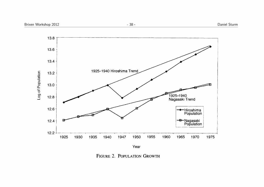
• The following (famous) graph looks at the case of Hiroshima andNagasaki where 20.8 and 8.5 percent of the population areestimated to have died.
Brixen Workshop 2012 - 38 - Daniel SturmTHE AMERICAN ECONOMIC REVIEW
c 0o
a. 0
o
1925 1930 1935 1940 1947 1950 1955 1960 1965 1970 1975
Year
FIGURE 2. POPULATION GROWTH
wartime growth should asymptotically ap- proach unity as the end period increases. In the last column of Table 3 we repeat the regression, only now extending the endpoint to 1965 in- stead of 1960. The estimated coefficient now reaches -1.027. That is, after controlling for prewar growth trends, by 1965 cities have en- tirely reversed the damage due to the war. Again, the impact of reconstruction subsidies also lessens as we move into the future. To- gether, these results suggest that the effect of the temporary shocks vanishes completely in less than 20 years.
One possible objection to our interpretation is that in most cases, the population changes cor- responded much more to refugees than deaths. Of the 144 cities with positive casualties, the average number of deaths per capita was only 1 percent. Most of the population movement that we observe in our data is due to the fact that the vast destruction of buildings forced people to live elsewhere. However, forcing them to move out of their cities for a number of years may not have sufficed to overcome the social networks and other draws of their home cities. Hence it may seem uncertain whether they are moving back to take advantage of particular character- istics of these locations or simply moving back to the only real home they have known.
However, there are two cases in which this argument cannot be made: Hiroshima and Na-
gasaki. In those cities, the number of deaths was such that if these cities recovered their popula- tions, it could not be because residents who temporarily moved out of the city returned in subsequent years. We have already noted that our data underestimates casualties in these cit- ies. Even so, our data suggest that the nuclear bombs immediately killed 8.5 percent of Na- gasaki's population and 20.8 percent of Hiro- shima's population. Moreover given that many Japanese were worried about radiation poison- ing and actively discriminated against atomic bomb victims, it is unlikely that residents felt an unusually strong attachment to these cities or that other Japanese felt a strong desire to move there. Another reason why these cities are in- teresting to consider is that they were not par- ticularly large or famous cities in Japan. Their 1940 populations made them the 8th and 12th largest cities in Japan. Both cities were close to other cities of comparable size so that it would have been relatively easy for other cities to absorb the populations of these devastated cities.
In Figure 2 we plot the population of these two cities. What is striking in the graph is that even in these two cities there is a clear indica- tion that they returned to their prewar growth trends. This process seems to have taken a little longer in Hiroshima than in other cities, but this is not surprising given the level of destruction.
1282 DECEMBER 2002

Brixen Workshop 2012 - 39 - Daniel Sturm
4.7 Implications
• The results of Davis and Weinstein (2002) show a stunningpersistence in city size even after horrific war-time devastation.
• This has important implications for attempts to use regional policyto shift economic activity between different spatial equilibria.
• This is summarized in the following quote from Davis andWeinstein (2002):

Brixen Workshop 2012 - 40 - Daniel Sturm
“An important practical question, then, is whether such spatialcatastrophes are theoretical curiosa or a central tendency in thedata. Our results provide an unambiguous answer: Even nuclearbombs have little effect on relative city sizes over the course ofa couple of decades. The theoretical possibility of spatialcatastrophes due to temporary shocks is not a central tendencyborne out in the data.” (Davis and Weinstein (2002), p. 1284)

Brixen Workshop 2012 - 41 - Daniel Sturm
4.8 Extensions
• The findings of Davis and Weinstein (2002) have been extended ina number of directions.
• Davis and Weinstein (2008) use data on the industry structure ofJapanese cities.
• They show that not only total population levels but also theindustrial composition of cities recovers quickly after the war.
• Brackman et. al. (2004) replicate the analysis of Davis andWeinstein (2002) on West German data.
• They find that also in this context cities recover quickly from thewar-time shock (but their results are not as clear cut).

Brixen Workshop 2012 - 42 - Daniel Sturm
• Another application of this idea is Miguel and Roland (2011), wholook at the case of Vietnam.
“The United States Air Force dropped in Indochina, from 1964to August 15, 1973, a total of 6,162,000 tons of bombs andother ordnance. U.S. Navy and Marine Corps aircraft expendedanother 1,500,000 tons in Southeast Asia. This tonnage farexceeded that expended in World War II and in the KoreanWar. The U.S. Air Force consumed 2,150,000 tons of munitionsin World War II 1,613,000 tons in the European Theater and537,000 tons in the Pacific Theater and 454,000 tons in theKorean War.” (Clotfelder (1995) as citied in Miguel and Roland(2011))

Brixen Workshop 2012 - 43 - Daniel Sturm
4.9 Conclusion
• The evidence presented in the literature following Davis andWeinstein (2002) is extremely powerful.
• Spatial patterns seem to be highly persistent and resilient toshocks of horrific magnitudes.
• This should give pause to policy-makers who attempt to usetemporary policy interventions to shift the economy betweendifferent equilibria.

Brixen Workshop 2012 - 44 - Daniel Sturm
•While the use of bombing as a temporary shock is ingenious, italso has a number of potential problems:
– Even though bombing kills people and destroys housing andsocial networks it does not destroy legal titles and operatingpermits.
– As a result rebuilding cities may simply be easier than starting anew settlement from scratch.
– Similarly, even after a nuclear blast there is going to beremaining useful infrastructure, which may make it cheaper torebuild in the old location.
Brixen Workshop 2012 - 45 - Daniel Sturm
5 Empirical Testing: German division
• Redding, Sturm and Wolf (2011) use an alternative naturalexperiment to bombing to investigate the impact of temporaryshocks: German division and reunification.
• Key idea: Does economic activity which was relocated in responseto division returns to its pre-war pattern after reunification.
• They focus on a particular industry which is both likely to be proneto multiple steady-states and for which a wealth of data isavailable: air transportation.

Brixen Workshop 2012 - 46 - Daniel Sturm
5.1 Road Map
• Sketch of the theoretical model
• Data and empirical strategy
• Basic finding
• Further evidence
• Conclusion

Brixen Workshop 2012 - 47 - Daniel Sturm
5.2 Theoretical Model
• There are three cities and demand for air travel between any twocities is a decreasing function of the price (derived frommicro-foundations in the paper).
• There is a monopoly airline which has to choose whether toconnect all three cities directly or to use one city as a “hub”.
• The airline’s marginal costs depend on distance flown and it has topay a fixed cost F > 0 for any bilateral connection.
• Finally, creating a hub involves sunk costs H > 0.

Brixen Workshop 2012 - 48 - Daniel Sturm
5.3 Basic Implications of the Model
• Operating a hub based in city i will generate higher per-periodprofits if the saving in fixed costs F exceeds the loss in variableprofits due to the longer distance flown on indirect connections:
ωi = F−(
πDkj − π I
kj
)•Without loss of generality index cities so that ω1 ≥ ω2 ≥ ω3.
• Denote the corresponding present discounted values byΩ1 ≥ Ω2 ≥ Ω3.

Brixen Workshop 2012 - 49 - Daniel Sturm
• There are multiple steady-state hub locations if for several cities i:
Ωi > H and Ωj−Ωi < H ∀j 6= i
• In contrast, the equilibrium hub location is unique if for one city i:
Ωi > H, and Ωi −Ωj > H ∀j 6= i
• Therefore, the existence of multiple steady-state locations dependson the size of the sunk cost relative to variation in economicfundamentals.

Brixen Workshop 2012 - 50 - Daniel Sturm
5.4 Temporary Shocks
• Suppose parameters are such that city one and two are potentialequilibrium locations for the hub and the hub is located in city one.
• A shock S such as division will shift the location of the hubbetween multiple equilibria if:
– It is large enough to relocate the hub: Ω2− (Ω1− S) > H– It is ultimately reversed to an extent that both locations are
again potential equilibria: |Ω2− (Ω1− S′)| < H
Brixen Workshop 2012 - 51 - Daniel Sturm
5.5 Data
• The basic dataset consists of the number of departing passengersat the major German airports from 1927 - 1938 and 1950 - 2002.
• Additional datasets are:
– Departing passengers at the largest European airports in 1937and 2002.
– Economic characteristics of the locations of major Germanairports.
– Bilateral passenger flows between the major German airportsand all worldwide destinations in 2002.
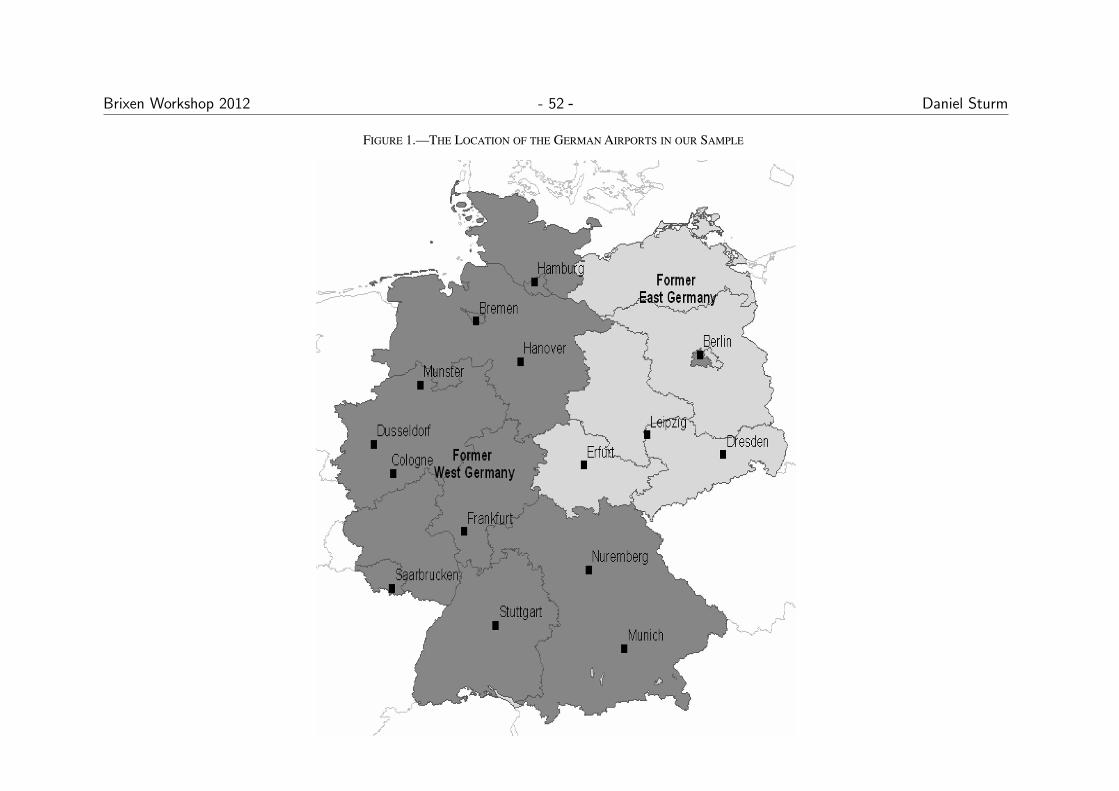
Brixen Workshop 2012 - 52 - Daniel SturmHISTORY AND INDUSTRY LOCATION: EVIDENCE FROM GERMAN AIRPORTS 819
Figure 1.—The Location of the German Airports in our Sample
a relatively short period of time over which to observe theimpact of the exogenous shock. For this reason, we concen-trate on statistical tests based on changes in airports’ trendrates of passenger growth.12
V. Basic Empirical Results
A. Evolution of Airport Passenger Shares
Before we estimate our basic specification, figure 2 dis-plays the share of the ten largest German airports in totaldepartures at these airports over the period 1927 to 2002. Thisgraph reveals a number of striking patterns. Before WorldWar II, Berlin had the largest airport in Germany by a sub-stantial margin and was in fact the largest airport in Europein 1937 in the historical data used in section VIA. By 1927,when the data shown in figure 2 start, Berlin had more thantwice as large a market share as the next largest Germanairport. From 1931 onward, a period of rapid growth in airtraffic at all German airports, Berlin’s market share steadilyincreased and reached a peak of over 40% in 1938. The four
12 Reestimating equation (5) allowing only changes in intercepts betweenthe prewar, division, and reunification periods yields a similar pattern ofresults.
airports ranked after Berlin are Frankfurt, Munich, Hamburg,and Cologne. These airports had very similar market shares,which remained remarkably stable at around 10% throughoutthe prewar period.
The dominance of Berlin in German air traffic changed dra-matically after the division of Germany. While Berlin wasstill the largest airport in Germany in terms of total depar-tures in 1950, when data became available again, Frankfurtwas already the second largest airport, substantially ahead ofHamburg and Munich. Over the next decade, Berlin steadilydeclined in importance, and by 1960 Frankfurt overtookBerlin as the largest German airport.13 A further accelera-tion in the decline of Berlin’s share occurred immediatelyafter 1971, when the Transit Agreement between East andWest Germany substantially improved road and rail con-nections between West Berlin and West Germany. By the
13 The spike in departures in 1953 in Berlin is mainly due to a wave ofrefugees leaving East Germany via West Berlin after the violent uprisingsin East Germany in June 1953. The Statistical Yearbook of West Germanyreports that 257,308 East German refugees left West Berlin by plane in1953, which accounts for as much as 47% of total departures in Berlin inthis year. Between 1954 and 1960, this stream of East German refugeesdeparting from West Berlin by plane continued at a rate of approximately95,000 people per year, which accounted for on average 16% of departuresin Berlin. It ceased with the building of the Berlin Wall in 1961.

Brixen Workshop 2012 - 53 - Daniel Sturm820 THE REVIEW OF ECONOMICS AND STATISTICS
Figure 2.—Airport Passenger Shares
Departing Passengers at the Ten Main German Airports
1980s, Frankfurt and Berlin had almost exactly changed roles.Frankfurt in the 1980s had a stable market share between 35%and 40%, while Berlin’s market share was just below 10%.
In contrast to the striking change in the pattern of air traf-fic following division, there was hardly any visible impactof reunification. The small step increase in Berlin’s share ofpassenger traffic in 1990 is due to the fact that we aggre-gate departures from Tempelhof and Tegel (in West Berlin)and Schoenefeld (in East Berlin) from this year onward.Apart from this small step increase, the trend in Berlin’sshare of passenger traffic has been slightly negative sincereunification. At the same time, Frankfurt clearly remainsGermany’s leading airport. Its share of passenger traffichas remained virtually flat since reunification, if anythingincreasing marginally.14
Although there is no evidence so far of a return towardprewar patterns of passenger traffic, is there any expecta-tion of a future relocation of Germany’s air hub to Berlin?Berlin plans to open a new airport around 2012, which willreplace the current system of three airports that together havean annual capacity of about 7.5 million departing passen-gers. The new airport is designed to have a starting capacityof approximately 10 million departing passengers. Around2015, Frankfurt airport plans to open a third passenger termi-nal, which will increase the airport’s capacity from its current28 million departing passengers a year by approximately
14 We see a similar pattern in freight departures. Following division, Frank-furt replaced Berlin as Germany’s leading airport for freight, and there wasagain no visible impact of reunification. Berlin’s average share in totalfreight departures fell from 36.5% to 0.7% between the ten years leadingup to 1938 and the ten years leading up to 2002. Over the same period,Frankfurt’s average share increased from 11.2% to 70.6%.
another 12.5 million passengers.15 Therefore, over the com-ing years, Frankfurt plans to increase its capacity by an evenlarger amount than Berlin’s overall capacity, which illustratesthat there is little expectation of a return of Germany’s air hubto Berlin.
B. Difference-in-Differences Estimates
To examine the statistical significance of the changesshown in figure 2, table 1 reports results for our baselinespecification, equation (5). The coefficients on the time trendsin each airport in each period capture mean annual rates ofgrowth of passenger shares. The final column of panel A oftable 2 compares the time trends between the prewar anddivision periods for Berlin and Frankfurt (a difference withinairports across periods) and shows that Berlin’s mean rate ofgrowth of passenger shares declined by 2.7 percentage pointsper annum, while Frankfurt’s rose by 0.4 percentage pointsper annum. Both changes are highly statistically significant.16
We next consider the statistical significance of the dif-ference in time trends between Berlin and Frankfurt withinthe prewar and division periods (a difference within periodsacross airports). The final row of panel A of table 2 showsthat within each period, the difference in the mean annual
15 These numbers are taken from http://www.berlin-airport.de andhttp://www.ausbau.flughafen-frankfurt.de. While we report capacity as thenumber of departing passengers, airports often report their capacity as thesum of arriving and departing passengers, which is simply twice the capacityfor departing passengers.
16 As is evident from figure 2, the within-airport change in time trendsfor Frankfurt understates its rise between the prewar and division periods,since some of the rise in Frankfurt’s postwar share of passenger traffic hadalready occurred prior to 1950 when data become available (and is thereforecaptured in Frankfurt’s intercept for the division period).

Brixen Workshop 2012 - 54 - Daniel Sturm
5.6 Further Evidence
• The evidence presented so far is suggestive that there has been ashift between multiple steady-state locations.
• An alternative explanation is that economic fundamentals havechanged so much between the pre-war and reunification periodsthat Berlin is no longer a potential equilibrium hub location.
• There are several additional pieces of evidence to rule out thisalternative explanation.

Brixen Workshop 2012 - 55 - Daniel Sturm
5.6.1 Comparison with other Countries
• As the table on the next slide shows, the experience of Germany ishighly unusual.
• In all other countries the largest airport before the war is also thelargest airport today (and is in the largest city).

Brixen Workshop 2012 - 56 - Daniel Sturm
822 THE REVIEW OF ECONOMICS AND STATISTICS
Table 3.—The Largest Airports of European Countries, 1937 and 2002
(1) (2) (3) (4)Market Share of Market Share of Rank of Largest
Largest Airport, Largest Airport, Largest Airport, Airport 1937 in1937 1937 2002 2002
Austria Vienna 94.1 76.5 1Belgium Brussels 65.6 89.9 1Denmark Copenhagen 96.2 91.7 1Finland Helsinki 80.3 73.7 1France Paris 70.2 61.4 1Germany Berlin 30.8 35.0 4Greece Athens 43.9 34.7 1Ireland Dublin 100.0 78.1 1Italy Rome 35.7 34.5 1Netherlands Amsterdam 62.3 96.4 1Norway Oslo 75.6 45.8 1Portugal Lisbon 100.0 46.3 1Spain Madrid 43.5 26.8 1Sweden Stockholm 56.9 61.9 1Switzerland Zurich 55.7 62.0 1United Kingdom London 52.7 65.6 1
The countries are the EU 15 countries without Luxembourg (which had no airport prior to World War II and had only one airport in 2002) and Norway and Switzerland. The prewar data for Austria refer to the year1938. The prewar data for Spain are the average over 1931 to 1933. As in the case of Berlin, we aggregate airports when cities have more than one airport. See the data appendix for detailed references to the sources.
country’s largest airport in 1937, the market share of thelargest airport in 1937, the market share of the largest airportin 2002, and the rank of the largest 1937 airport in 2002.17
Although there are many differences in the technology andstructure of air traffic between the prewar and present-dayperiods, the first striking feature of the table is that Germany isthe only country where the leading airport in 1937 was not theleading airport in 2002 (Berlin ranked fourth in 2002). In allother countries, there is a perfect correlation between the pastand current locations of the leading airport. The 1937 airportmarket shares are not only qualitatively but also quantitativelygood predictors of the 2002 airport shares. There is a positiveand highly statistically significant correlation between thepast and current market shares, and we are unable to rejectthe null hypothesis that the 2002 market shares equal their1937 values.18 The remarkable persistence in the location ofthe leading airport in European countries suggests that thereis little secular change in the location of such airports.
Apart from the stability in the identity and market shareof a country’s leading airport over time, there is also a sim-ilarity over time in the shares of direct connections servedby a country’s leading airport relative to the shares servedby other airports. In the case of Germany, Berlin in 1935served 72% of all destinations served by any other Germanairport, more than twice Frankfurt’s share of 31%. A similarpattern is observed in 2002: Frankfurt served 95% of all des-tinations served by any other German airport, nearly twiceBerlin’s share of 55%. Further informal evidence that Frank-furt’s current dominance was mirrored in Berlin’s prewar
17 The countries are the EU 15, Norway, and Switzerland but excludingLuxembourg, which did not have an airport prior to World War II, and, dueto its size, has only one airport today.
18 If the 2002 market shares are regressed on the 1937 market sharesexcluding the constant, we are unable to reject the null hypothesis that thecoefficient on the 1937 market shares is equal to 1 (p-value = 0.162).
dominance comes from contemporary observers. Accord-ing to Sefton Brancker, director general for civil aviationwithin the British Air Ministry, Germany led Europe in termsof the development of civil aviation from the mid-1920sonward (Myerscough, 1985), and Berlin was Europe’s prewaraviation hub (Luftkreuz Europas, cited in Weise, 1928).
Finally, a comparison between Germany and other Euro-pean countries reveals that Germany is the only country wherethe largest airport is not currently located in the largest city.In all other European countries, there is a perfect correspon-dence between the location of the largest airport and thelocation of the largest city. Taken together, these findingssupport the idea that in the absence of division, Germany’slargest airport would be located today in Berlin and that itis at least not obvious that Berlin, Germany’s largest cityby a substantial margin, can be excluded as a possible hublocation.
B. The Selection of Frankfurt
An important question about the relocation of Germany’sair hub after division is why it moved to Frankfurt ratherthan some other location. As evident from figure 2, there isa remarkable similarity in prewar shares of air traffic amongFrankfurt, Cologne, Hamburg, and Munich. From this pat-tern of prewar passenger departures, it would be difficult topredict that Frankfurt, rather than one of these other airports,would rise to replace Berlin as Germany’s leading airportafter division. To the extent that differences in fundamentalsare reflected in differences in passenger departures, this sug-gests that Frankfurt did not enjoy superior fundamentals tothese other potential locations prior to division.
Instead Frankfurt’s rise probably owes much to a numberof small historical accidents. In contrast to Cologne and Ham-burg, Frankfurt was located in the U.S. occupation zone, andin 1948 it was chosen as the European terminal for the U.S.

Brixen Workshop 2012 - 57 - Daniel Sturm
5.6.2 The Role of Market Access
• The model suggests that bilateral departures depend on:
– Remoteness from other locations (market access)
– Local economic fundamentals (in particular population)
– An airport’s role as a hub.
• The contribution of market access can be estimated with the helpof a gravity model.

Brixen Workshop 2012 - 58 - Daniel Sturm
• In particular one can estimate:
ln(
Aij
)= si + mj + δ ln
(distij
)+ uij
• The estimated coefficients can be used to decompose totalpassenger departures as follows:
Ai = ∑j
Aij = SiMAi where MAi = ∑j
distδijMj

Brixen Workshop 2012 - 59 - Daniel SturmHISTORY AND INDUSTRY LOCATION: EVIDENCE FROM GERMAN AIRPORTS 825
Figure 3.—The Role of Market Access
The estimates of market access and the source airport fixed effects are derived from the gravity equation (6) for bilateral passenger departures. The log deviations from Berlin for market access and the source airportfixed effects sum to the log deviation from Berlin for fitted total departures.
using a Poisson fixed-effects specification (see Silva & Ten-reyro, 2006). Also in this specification, we find that marketaccess contributes little to explaining Frankfurt’s dominanceof German air travel.
D. Local Economic Activity and Local Departures
Having shown that market access makes a relatively smallcontributiontowardexplainingdifferencesinpassengerdepar-tures across airports, we now examine the model’s other keydeterminant of the attractiveness of an airport as a hub: localeconomic activity. To do so, we begin by decomposing totalpassenger departures from each airport into local departuresthat originate in the vicinity of the airport and various formsof transit traffic. Using this decomposition, we then examinethe relationship between local departures and local economicactivity, as well as the variation in local economic activityacross alternative potential locations for Germany’s air hub.
We decompose total passenger departures from each Ger-man airport into four components: (a) international air transitpassengers, who are changing planes at the airport en routefrom a foreign source to a foreign destination; (b) domesticair transit passengers, who are changing planes at the airportand have either a source or final destination within Germany;(c) ground transit passengers, who arrived at the airport usingground transportation and who traveled more than 50 kilome-ters to reach the airport; and (d) local passengers, who arrivedat the airport using ground transportation and who traveledless than 50 kilometers to reach the airport.
To undertake this decomposition, we combine data on airtransit passengers collected by the German Federal Statis-tical Office with information from a harmonized survey ofdeparting passengers at all major German airports in 2003
coordinated by the German Airports Association (Arbeitsge-meinschaft Deutscher Verkehrsflughäfen). Although the dis-aggregated results of the survey of departing passengers areproprietary data, Wilken, Berster, and Gelhausen (2007) con-struct and report a number of summary results. These includethe share of all departing passengers from each German air-port whose journey began within 50 kilometers of the airport,which ranges from 85% in Berlin to 37% in Frankfurt, withan average of 59% across the fifteen airports.
Figure 4 breaks out total departures at the German airportsin 2002 into the contributions of these four categories of pas-sengers. The panels display total departures, total departuresminus international air transit passengers, total departuresminus all air transit passengers, and total departures minusall air and ground transit passengers (i.e., local departures).Total departures (top left panel) vary substantially acrossairports: from 0.2 million in Saarbrucken to nearly 24.0 mil-lion in Frankfurt. Simply subtracting international air transitpassengers from total departures (top right panel) substan-tially reduces the extent of variation: from 0.2 million inSaarbrucken to 16.4 million in Frankfurt.
Since international air transit passengers are en route froma foreign source to a foreign destination and are merelychanging planes within Germany, this category of passengersseems most closely connected with an airport’s hub status.International air transit passengers alone account for around32% of Frankfurt’s total departures, and Frankfurt accountsfor around 82% of international air transit passengers inGermany.24 Therefore, Frankfurt’s hub status clearly plays
24 The only other airport with a nonnegligible share of international airtransit passengers is Munich, which has developed over the past two decadesinto a much smaller secondary hub. International air transit passengersaccount for 14% of Munich’s total departures, and Munich’s share of thiscategory of passengers in Germany is 17%.
Brixen Workshop 2012 - 60 - Daniel Sturm
5.6.3 What Explains the Size of Frankfurt?
• Frankfurt’s size is almost entirely due to its status as a transit hub.
• Furthermore economic fundamentals affect the volume of traffic inthe way suggested by the model.

Brixen Workshop 2012 - 61 - Daniel Sturm826 THE REVIEW OF ECONOMICS AND STATISTICS
Figure 4.—Transit and Local Passenger Departures, 2002
International air transit passengers are those changing planes at an airport en route from a foreign source to a foreign destination. Domestic air transit passengers are those changing planes at an airport with either asource or destination within Germany. Ground transit passengers are those who traveled more than 50 kilometers to an airport using ground transporation. See the data appendix for further discussion of the data sources.
a major role in understanding its dominance of German pas-senger traffic. This conclusion is strengthened by subtractingboth international and domestic air transit passengers fromtotal departures (bottom left panel). Together the two cate-gories of air transit passengers account for 49% of Frankfurt’stotal passenger departures, and Frankfurt accounts for 75%of all air transit passengers in Germany.25
Moving to local departures in the bottom right panel (sub-tracting both air and ground transit passengers from totaldepartures) entirely eliminates Frankfurt’s dominance of Ger-man air travel: 4.55 million passengers originated from within50 kilometers of Frankfurt airport, compared to 4.23 millionfor Munich, 4.28 for Dusseldorf, and 5.07 million for Berlin.This decomposition suggests that Frankfurt’s much highervolume of passenger traffic than Berlin, Munich, or Dussel-dorf is due to its larger volume of transit traffic and not alarger volume of passenger traffic originating from withinthe immediate vicinity of the airport.
While variation in local departures cannot explain Frank-furt’s dominance of German air travel, figure 5 shows that thiscategory of passengers is closely related to local economicactivity, as suggested by the theoretical model. The figureplots the logarithm of the number of passengers originatingwithin 50 kilometers of each airport against the logarithmof GDP within 50 kilometers of each airport, as well as thelinear regression relationship between the two variables.26
25 The corresponding numbers for Munich are 28% of the airport’s totaldepartures and 20% of all air transit passengers in Germany.
26 GDP within 50 kilometers of an airport is calculated from the populationof all municipalities (Gemeinden) within 50 kilometers of the airport andthe GDP per capita of the counties (Kreise) in which the municipalities arelocated. See the data appendix for further discussion.
The figure shows a tight relationship between local passen-ger volumes and local GDP. Over 80% of the variation inlocal departures is explained by the regression, and thecoefficient on local GDP is highly statistically significant.27
One notable feature of figure 5 is that Cologne and Dussel-dorf have greater concentrations of local economic activitythan Frankfurt, and the difference in local economic activ-ity between Frankfurt and Berlin is in fact around the samemagnitude as between Frankfurt and Dusseldorf. This find-ing parallels our discussion in section VIB, where we notedthat several other German airports had similar levels of pre-war passenger traffic to Frankfurt. From the concentrationsof local economic activity shown in figure 4, it also seemsdifficult to conclude that Frankfurt is the only possible loca-tion for Germany’s air hub. A similar picture also emergesfrom the headquarters data that we used in section VIC for ourgravity estimation. In these data, Frankfurt is ranked fourth interms of the number of headquarters, after Hamburg, Berlin,and Munich.
To further reinforce the point that Frankfurt is not nec-essarily the most attractive location for Germany’s air hub,figure 6 places our fifteen airports in the context of the dis-tribution of GDP within 50 kilometers of every German citywith more than 50,000 inhabitants in 2002.28 The figure dis-plays the log rank – log size relationship for this distributionand labels the cities in which the fifteen German airports are
27 The estimated coefficient (standard error) on local GDP is 1.592 (0.237).Regressing local passenger departures on population (instead of GDP)within 50 kilometers of an airport yields a similar pattern of results.
28 As discussed above, GDP within 50 kilometers is calculated from thepopulation of all municipalities within 50 kilometers of a city and the GDPper capita of the counties in which those municipalities are located.

Brixen Workshop 2012 - 62 - Daniel SturmHISTORY AND INDUSTRY LOCATION: EVIDENCE FROM GERMAN AIRPORTS 827
Figure 5.—Local Departures and Local GDP
Local departures are those who traveled less than 50 kilometers to an airport. Local GDP is calculated from the population of all municipalities within 50 kilometers of an airport and the GDP per capita of the countiesin which the municipalities are located. The three-letter codes are: BLN: Berlin; BRE: Bremen; CGN: Cologne, DUS: Dusseldorf; DRS: Dresden; ERF: Erfurt; FRA: Frankfurt; HAM: Hamburg: HAJ: Hanover; LEJ:Leipzig; FMO: Munster; MUC: Munich; NUE: Nuremberg; SCN: Saarbrucken; STR: Stuttgart.
Figure 6.—Local GDP for German Cities, 2002
Figure displays German cities with a population greater than 50,000. Local GDP is the sum of GDP in all municipalities whose centroids lie within 50 kilometers of the centroid of a city. Municipality GDP isconstructed using municipality population and GDP per capita in the county where the municipality is located. Rank is defined so that the city with the largest local GDP has a rank of 1. See the note to figure 5 for thelist of three-letter codes.
located.29 As apparent from the figure, the fifteen airports arenot necessarily located in the cities with the greatest local con-centrations of economic activity. Furthermore, the thirty citieswith the greatest concentrations of local economic activitywithin 50 kilometers are all located in the Rhine-Ruhr region
29 As in the literature concerned with population-size distributions (see,for example, Rossi-Hansberg & Wright, 2007), we find departures fromthe linear relationship between log rank and log size implied by a Paretodistribution. The concave relationship shown in the figure implies thinnertails than a Pareto distribution.
of northwest Germany, which includes Cologne and Dussel-dorf. Frankfurt, located to the south in the Rhine-Main regionof western Germany, is ranked 42.30
E. Quantifying Differences in Profitability across Locations
While the previous two sections have shown that differ-ences in market access and local economic activity acrossour fifteen airports appear to be small relative to differences
30 We find a similar pattern of results for population within 50 kilometers.

Brixen Workshop 2012 - 63 - Daniel Sturm
5.6.4 Simulating the Impact of Moving the Hub
• The final piece of evidence is a simulation of the impact ofrelocating the hub on volumes of four types of passengers:
– International Transits
– Domestic Transits
– Ground Transits
– Local Departures
• Table 5 summarizes the impact of relocating the hub.

Brixen Workshop 2012 - 64 - Daniel Sturm
HISTORY AND INDUSTRY LOCATION: EVIDENCE FROM GERMAN AIRPORTS 829
Table 5.—Estimated Impact of Relocating the Air Hub from Frankfurt on Total Passenger Departures across the 15 German airports
(1) (2) (3) (4)Estimated Change in Estimated Change in Estimated Change in Estimated Percentage
Alternative Location of Air Transit Ground Transit Total Passenger Change in Totalthe Air Hub Passengers Passengers Departures Passenger Departures
Berlin −407,498 −1,862,056 −2,232,380 −3.38Dusseldorf 148,590 − 18,331 125,759 0.19Hamburg −332,672 −1,644,620 −1,852,323 −2.80Munich 566,039 − 865,146 − 422,204 −0.64
The table reports the estimated change in passenger departures across the 15 German airports as a result of the hypothetical relocation of the air hub from Frankfurt to each of the alternative locations. All air transitpassengers who currently change planes at Frankfurt are assumed to instead fly via the alternative airport, and the coefficient on distance from column 4 of table 4 is used to infer the change in the number of air transitpassengers as a result of the change in distance traveled caused by the relocation of the hub. The logarithm of ground transit departures is regressed on the logarithm of the distance-weighted sum of GDP in all Germancounties, and the estimated coefficient is used to infer how the number of ground departures currently observed in Frankfurt would change if it instead had the distance-weighted GDP of the alternative location of thehub. See the main text for further discussion. Total bilateral departures for the 15 German airports in 2002 were 66,134,047. Total bilateral departures from Frankfurt airport in 2002 were 23,782,604.
a change in total passengers by 2.5 million (which is largerthan any of the changes in table 5) would be 0.86 billioneuros. In comparison, the construction costs of the new ter-minal facilities in Berlin, which are at best one-third of thesize necessary to replace Frankfurt, are projected to be around2 billion euros.36
Our analysis of the impact of relocating the hub fromFrankfurt to another German airport clearly makes a num-ber of simplifying assumptions and assumes that apart fromthe relocation of transit traffic from Frankfurt to an alternativeairport, the structure of German air traffic remains unchanged.Despite these caveats, the stark difference between theimplied change in the net present value of profits and plausi-ble estimates for the sunk costs of creating the hub suggeststhat it is unlikely the difference in profitability across alterna-tive locations for the air hub in Germany outweighs the largesunk costs of creating the hub. This reinforces the conclusionthat several other locations apart from Frankfurt, includingBerlin, are potential steady state locations for Germany’s airhub.
VII. Conclusion
While a central prediction of a large class of theoreticalmodels is that industry location is not uniquely determinedby fundamentals, there is a surprising scarcity of empiricalevidence on this question. In this paper, we exploit the com-bination of the division of Germany in the wake of WorldWar II and the reunification of East and West Germany in1990 as a natural experiment to provide empirical evidencefor multiple steady states in industry location. We find thatdivision results in a relocation of Germany’s leading airportfrom Berlin to Frankfurt, but there is no evidence of a returnof the leading airport to Berlin in response to reunification.
To provide evidence that this change in location is indeeda shift between multiple steady states, we compare Germanywith other European countries, use data on prewar passen-ger shares, examine the determinants of bilateral departuresfrom German airports to destinations worldwide, and exploitinformation on the origin of passengers departing from eachGerman airport. We show that Frankfurt’s rise to becomeGermany’s postwar air hub is difficult to predict based on
36 This estimate is taken from http://www.berlin-airport.de/DE/BBI/.
either prewar passenger shares or current economic funda-mentals. We quantify the impact of differences in economicfundamentals on both transit activity and local departures andshow that the predicted changes in the net present values ofprofits across alternative potential locations for Germany’sair hub are small relative to the sunk costs of creating thehub. All of the available evidence therefore suggests that thelocation of an air hub is not uniquely determined by funda-mentals and that there is instead a range of possible steadystate locations for the hub for which differences in economicfundamentals are dominated by the substantial sunk costs ofcreating the hub.
While the main focus of our research has been to find anatural experiment for which we can provide compelling evi-dence in support of multiple steady states in industry location,our findings also have broader implications for the abilityof public policy and other interventions to influence loca-tion choices. The sheer magnitude of German division andthe length of time that it took for Frankfurt and Berlin toexchange places as Germany’s air hub suggest that the typeof intervention required to dislodge an established steadystate needs to be not only large but also sufficiently persistentto influence forward-looking location decisions. This offerssupport for those who are pessimistic about the ability ofrealistic interventions to dislodge an economic activity froman existing steady state. However, the similarity of prewarpassenger shares and also current economic fundamentalsbetween Frankfurt and several other locations within Ger-many suggest that Frankfurt’s subsequent rise to becomeGermany’s air hub was by no means a forgone conclusion.Therefore, there may be substantially more scope for rela-tively small interventions, such as the U.S. military’s decisionto make Frankfurt their main postwar European air transportbase, to influence location decisions before a new steady statehas become established.
REFERENCES
Airports Council International, “Worldwide Airport Traffic Report,”www.airports.org (2002).
Amiti, M., and L. Cameron, “Economic Geography and Wages,” thisreview 89 (2007), 15–29.
Arbeitskreis Volkswirtschaftliche Gesamtrechnung der Länder, “Brut-toinlandsprodukt, Bruttowertschöpfung in den kreisfreien Städtenund Landkreisen Deutschlands 1992 und 1994 bis 2003,” http://www.statistik.baden-wuerttemberg.de/Arbeitskreis_VGR/ (2005).

Brixen Workshop 2012 - 65 - Daniel Sturm
• At 10 Euro per passenger and a 3 percent discount rate the NPVof a change in the total passenger volume by 2.5 million would be0.86 billion Euro.
• The construction of new terminal facilities at Berlin which aredesigned to be a third of the size of Frankfurt were estimated tocost just over 2 billion Euro (current costs >4.5 billion Euro).
• A third runway at Heathrow is currently costed at 10 billionPounds.

Brixen Workshop 2012 - 66 - Daniel Sturm
5.7 Why Frankfurt?
• Several historical accidents propelled Frankfurt ahead of alternativelocations for the hub in the post-war period:
– Frankfurt airport was captured by U.S. troops in March 1945.
– From 1948 Frankfurt became the European terminal for theU.S. Military Air Transport Service (MATS).
– During the Berlin airlift of 1948-9, Frankfurt was theoperational center for the U.S. contribution to the airlift.

Brixen Workshop 2012 - 67 - Daniel Sturm
5.8 Conclusion
• Redding, Sturm and Wolf (2011) show that German division eventhough ultimately temporary seems to have permanently movedthe location of Germany’s hub airport.
• They present a number of pieces of evidence that this shift is dueto a shift between equilibria rather than a change in fundamentals.
• The rise of Frankfurt was a long process and it is not clear thatFrankfurt would have survived as the new hub if reunification hadhappened in the early 1960s.
• This suggests that for temporary shocks to permanently changelocation decisions they need to be fairly long-lasting.

Brixen Workshop 2012 - 68 - Daniel Sturm
•While the paper provides suggestive evidence there are least twoopen questions:
– To what extent are economic activities other than air hubssubject to multiple equilibria?
– What policy instruments could generate the same impact asGerman division?

Brixen Workshop 2012 - 69 - Daniel Sturm
6 Empirical Testing: Portage
• In a paper that has just been published in the QJE Bleakley andLin use a somewhat different empirical approach to the question offundamentals versus agglomeration and path dependence.
• They do not look for another kind of temporary shock.
• Instead they investigate the impact of a natural feature that wasvalued historically but has become obsolete a long time ago.
• In particular they look at so called “portage” sites.

Brixen Workshop 2012 - 70 - Daniel Sturm
• Portage refers to the carrying of boats or their cargo over land toavoid obstacles such as rapids or water falls.
• During the early settlement of the US most goods traveled by boaton rivers and portage sites were natural places for exchange andcommerce.
• However, the importance of portage sites vanished with theconstruction of canals and the railroads.
• Proximity to a portage site has been economically irrelevant for atleast 100 years.
• This is illustrated in the following graph.

Brixen Workshop 2012 - 71 - Daniel SturmPORTAGE AND PATH DEPENDENCE 597
FIGURE IWater-Transportation Employment across Fall-Line-Area Counties, 1850–1930
This figure displays employment in water transportation (e.g., stevedoringoccupations) across 51 historical portage sites between 1850 and 1930. We ag-gregate microdata from eight IPUMS extracts based on county of residence andwater transportation employment in the IPUMS-recoded variable ind1950=546.Twohistorical portage sites, on the Schuylkill andthe Raritan rivers, are excludeddue to their continued use as seaports. Panel A shows the average share ofwater-transportation employment at historical portage sites, out of total water-transportation employment along each river. Panel B shows the average share ofwater-transportation employment out of total employment, in both portage (solid)and nonportage (dashed) counties adjacent to rivers.
at SWE
TS - T
rusted Agent G
ateway - O
UP on Septem
ber 16, 2012http://qje.oxfordjournals.org/
Dow
nloaded from

Brixen Workshop 2012 - 72 - Daniel Sturm
6.1 Data
• The paper uses three main datasets to measure the contemporarydensity of economic activity in different parts of the US:
– County level population
– Census tract population data from the 2000 census
– Nighttime light intensity data for 2003

Brixen Workshop 2012 - 73 - Daniel Sturm
6.2 Where Were Portage Sites?
• The paper considers three areas in which portage sites werelocated in the US.
• The most impressive and important of these is the so-called “fallline”.
• The following maps show the location of the fall line and economicactivity around the fall line.

Brixen Workshop 2012 - 74 - Daniel Sturm
PO
RT
AG
EA
ND
PA
TH
DE
PE
ND
EN
CE
641
FIGURE A.1The Density Near Fall-Line/River Intersections
This map shows the contemporary distribution of economic activity across the southeastern United States measured by the 2003nighttime lights layer. For information on sources, see notes for Figures II and IV.
at SWETS - Trusted Agent Gateway - OUP on September 16, 2012 http://qje.oxfordjournals.org/ Downloaded from

Brixen Workshop 2012 - 75 - Daniel SturmPORTAGE AND PATH DEPENDENCE 601
FIGURE IIFall-Line Cities from Alabama to North Carolina
The map in the upper panel shows the contemporary distribution of economicactivity across the southeastern United States, measured by the 2003 nighttimelights layer from NationalAtlas.gov. The nighttime lights are used to present anearly continuous measure of present-day economic activity at a high spatialfrequency. The fall line (solid) is digitized from Physical Divisions of the UnitedStates, produced by the U.S. Geological Survey. Major rivers (dashed gray) arefrom NationalAtlas.gov, based on data produced by the United States GeologicalSurvey. Contemporary fall-line cities are labeled in the lower panel.
We can see the importance of fall-line/river intersections bylooking along the paths of rivers. Along a given river, there istypicallya populatedplaceat thepoint wheretherivercrosses the
at SWE
TS - T
rusted Agent G
ateway - O
UP on Septem
ber 16, 2012http://qje.oxfordjournals.org/
Dow
nloaded from

Brixen Workshop 2012 - 76 - Daniel SturmPORTAGE AND PATH DEPENDENCE 605
FIGURE IVFall-Line Cities from North Carolina to New Jersey
The map in the left panel shows the contemporary distribution of economicactivity across the southeastern United States measured by the 2003 nighttimelights layer from NationalAtlas.gov. The nighttime lights are used to presenta nearly continuous measure of present-day economic activity at a high spatialfrequency. The fall line (solid) is digitized from Physical Divisions of the UnitedStates, produced by the U.S. Geological Survey. Major rivers (dashed gray) arefrom NationalAtlas.gov, based on data produced by the U.S. Geological Survey.Contemporary fall-line cities are labeled in the right panel.
rivers with smaller upstream watersheds such as Fredericksburgon the Rappahannock and Petersburg on the Appomattox, bothin Virginia. Minor settlements are also found on fall-line portagesites in North Carolina, but the relationship across sites betweenwatershed andpopulation is less evident. These rivers empty intotheAlbemarleandPamlicosounds, whichwereisolatedincolonialtimes from ocean-going commerce by the treacherous navigationnear and through the barrier islands. (Indeed, the area offshorewas the “Graveyard of the Atlantic.”)
V.B. Statistical Comparisons
Statistical tests confirm the features shown in the maps. Wefocus on two measures of initial portage advantage: (i) proximity
at SWE
TS - T
rusted Agent G
ateway - O
UP on Septem
ber 16, 2012http://qje.oxfordjournals.org/
Dow
nloaded from

Brixen Workshop 2012 - 77 - Daniel Sturm
602 QUARTERLY JOURNAL OF ECONOMICS
FIGURE IIIPopulation Density in 2000 along Fall-Line Rivers
These graphs display contemporary population density along fall-line rivers.We select census 2000 tracts whose centroids lie within 50 miles along fall-linerivers; the horizontal axis measures distance to the fall line, where the fall lineis normalized to zero, and the Atlantic Ocean lies to the left. In Panel A, thesedistances are calculated in miles. In Panel B, these distances are normalized foreach river relative tothe river mouth or the river source. The rawpopulation dataare then smoothed via Stata’s lowess procedure, with bandwidths of 0.3 (Panel A)or 0.1 (Panel B).
fall line. This comparison is useful in the following sense: today,all of the sites along the river have the advantage of being alongthe river, but only at the fall line was there an initial portage
at SWE
TS - T
rusted Agent G
ateway - O
UP on Septem
ber 16, 2012http://qje.oxfordjournals.org/
Dow
nloaded from

Brixen Workshop 2012 - 78 - Daniel Sturm
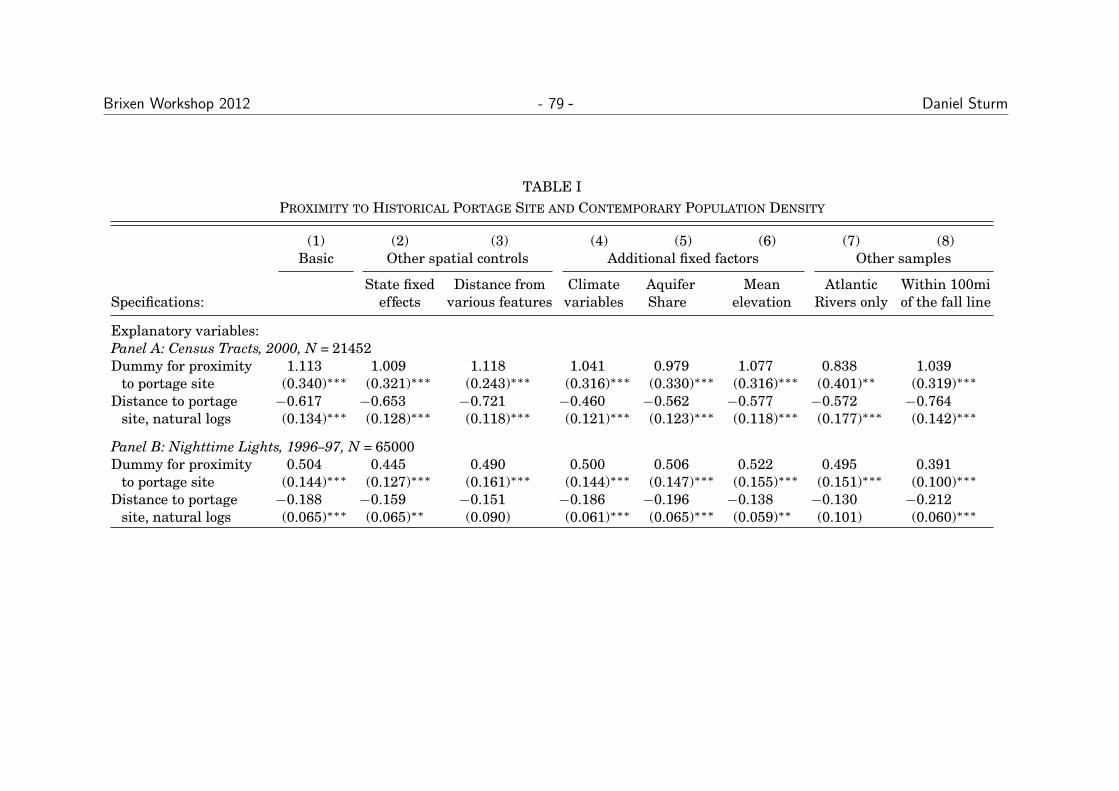
6.3 The Continuing Prominence of Portage Sites
• The maps on the previous slides show a striking pattern.
• The places at which the fall line intersects major rivers are alsotoday clearly visible agglomerations.
• Bleakley and Lin (2012) also provide statistical evidence that theseagglomerations are not random.
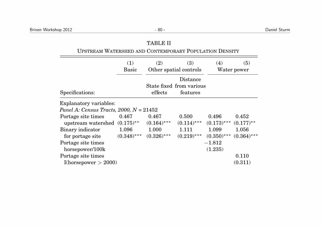
– The table on the next slide shows that portage sites have astatistically significantly higher density today.
– The following table shows that portages sites that served largerupstream areas are larger today.
Brixen Workshop 2012 - 79 - Daniel Sturm608
QU
AR
TE
RL
YJ
OU
RN
AL
OF
EC
ON
OM
ICS
TABLE I
PROXIMITY TO HISTORICAL PORTAGE SITE AND CONTEMPORARY POPULATION DENSITY
(1) (2) (3) (4) (5) (6) (7) (8)Basic Other spatial controls Additional fixed factors Other samples
Specifications:State fixed
effectsDistance from
various featuresClimatevariables
AquiferShare
Meanelevation
AtlanticRivers only
Within 100miof the fall line
Explanatory variables:Panel A: Census Tracts, 2000, N = 21452Dummy for proximity
to portage site1.113 1.009 1.118 1.041 0.979 1.077 0.838 1.039
(0.340)∗∗∗ (0.321)∗∗∗ (0.243)∗∗∗ (0.316)∗∗∗ (0.330)∗∗∗ (0.316)∗∗∗ (0.401)∗∗ (0.319)∗∗∗
Distance to portagesite, natural logs
−0.617 −0.653 −0.721 −0.460 −0.562 −0.577 −0.572 −0.764(0.134)∗∗∗ (0.128)∗∗∗ (0.118)∗∗∗ (0.121)∗∗∗ (0.123)∗∗∗ (0.118)∗∗∗ (0.177)∗∗∗ (0.142)∗∗∗
Panel B: Nighttime Lights, 1996–97, N = 65000Dummy for proximity
to portage site0.504 0.445 0.490 0.500 0.506 0.522 0.495 0.391
(0.144)∗∗∗ (0.127)∗∗∗ (0.161)∗∗∗ (0.144)∗∗∗ (0.147)∗∗∗ (0.155)∗∗∗ (0.151)∗∗∗ (0.100)∗∗∗
Distance to portagesite, natural logs
−0.188 −0.159 −0.151 −0.186 −0.196 −0.138 −0.130 −0.212(0.065)∗∗∗ (0.065)∗∗ (0.090) (0.061)∗∗∗ (0.065)∗∗∗ (0.059)∗∗ (0.101) (0.060)∗∗∗
at SWETS - Trusted Agent Gateway - OUP on September 16, 2012 http://qje.oxfordjournals.org/ Downloaded from
Brixen Workshop 2012 - 80 - Daniel SturmPORTAGE AND PATH DEPENDENCE 611
TABLE II
UPSTREAM WATERSHED AND CONTEMPORARY POPULATION DENSITY
(1) (2) (3) (4) (5)Basic Other spatial controls Water power
Specifications:State fixed
effects
Distancefrom various
features
Explanatory variables:Panel A: Census Tracts, 2000, N = 21452Portage site times
upstream watershed0.467 0.467 0.500 0.496 0.452
(0.175)∗∗ (0.164)∗∗∗ (0.114)∗∗∗ (0.173)∗∗∗ (0.177)∗∗
Binary indicatorfor portage site
1.096 1.000 1.111 1.099 1.056(0.348)∗∗∗ (0.326)∗∗∗ (0.219)∗∗∗ (0.350)∗∗∗ (0.364)∗∗∗
Portage site timeshorsepower/100k
−1.812(1.235)
Portage site timesI(horsepower> 2000)
0.110(0.311)
Panel B: Nighttime Lights, 1996–97, N = 65000Portage site times
upstream watershed0.418 0.352 0.456 0.415 0.393
(0.115)∗∗∗ (0.102)∗∗∗ (0.113)∗∗∗ (0.116)∗∗∗ (0.111)∗∗∗
Binary indicatorfor portage site
0.463 0.424 0.421 0.462 0.368(0.116)∗∗∗ (0.111)∗∗∗ (0.121)∗∗∗ (0.116)∗∗∗ (0.132)∗∗∗
Portage site timeshorsepower/100k
0.098(0.433)
Portage site timesI(horsepower> 2000)
0.318(0.232)
Panel C: Counties, 2000, N = 3480Portage site times
upstream watershed0.443 0.372 0.423 0.462 0.328
(0.209)∗∗ (0.185)∗∗ (0.207)∗∗ (0.215)∗∗ (0.154)∗∗
Binary indicator forportage site
0.890 0.834 0.742 0.889 0.587(0.211)∗∗∗ (0.194)∗∗∗ (0.232)∗∗∗ (0.211)∗∗∗ (0.210)∗∗∗
Portage site timeshorsepower/100k
−0.460(0.771)
Portage site timesI(horsepower> 2000)
0.991(0.442)∗∗
Notes. This table displays estimates of equation (2) in the text. Each column/panel presents estimatesfrom a separate regression. The baseline sample consists of all areas that are within the watersheds of riversthat cross the fall line. The estimator used is OLS, with standard errors clustered on the 53 watersheds. Theoutcome variables are, for Panel A, population density by census tracts from 2000; for Panel B, the intensityof nighttime lights; and, for Panel C, population data for counties from 2000. The basic specification includesa fourth-order polynomial in latitude and longitude, a set of fixed effects by the watershed of each riverthat crosses the fall line, dummies for proximity to the fall line and to a river, and the interaction of theselatter dummies with ln watershed area. The first portage-related variable in this table is the interaction ofthe portage site with the (demeaned) log of land area in the watershed upstream of the fall line, a variablethat proxies for historical demand for commerce at the portage site. The second portage-related variable isa binary indicator for proximity to the river/fall-line intersection. Column (3) controls for the natural log ofdistances to the fall line, to the ocean, to the closest river, and to the closest circa-1890 seaport. Columns (4)and (5) include controls for potential water-power at the fall line. Reporting of additional coefficients issuppressed. Data sources and additional variable and sample definitions are found in the text and theappendixes.
at SWE
TS - T
rusted Agent G
ateway - O
UP on Septem
ber 16, 2012http://qje.oxfordjournals.org/
Dow
nloaded from

Brixen Workshop 2012 - 81 - Daniel Sturm
6.4 Why Did Portage Sites Survive?
• There are two broad explanations why portage sites have survivednearly hundred years after portage has become irrelevant.
• One view is that the density of economic activity is determined byfundamentals.
• If this is the case, the decline in the importance of portage shouldeliminate portage sites in the long-run.
• The reason that this has not happened yet could be large sunkinvestments undertaken when portage was still important thatdepreciate slowly over time.
Brixen Workshop 2012 - 82 - Daniel Sturm
• An alternative view is that there are multiple spatial equilibria.
• Once established agglomerations of economic activity are heldtogether by the usual (second nature) agglomeration forces.
• The historical portage advantage has in this view only helped toselect an equilibrium location for an agglomeration from manypossible equilibria.

Brixen Workshop 2012 - 83 - Daniel Sturm
• The paper presents evidence that is consistent with multipleequilibria rather than a slow decline to the long-run equilibrium:
– Portage sites actually grow relative to other sites after portagebecomes irrelevant.
– Portage sites do not seem to have an excess supply of anyobvious factor of production (the historical sunk investment).

Brixen Workshop 2012 - 84 - Daniel SturmPORTAGE AND PATH DEPENDENCE 615
FIGURE VPortage and Population Density, 1790–2000
This graph displays estimates of equation (3) from repeated fixed-effectsregressions estimated separately by decade. Each regression uses county-yearobservations fromtheyearindicatedonthehorizontal axis and1850, thereferenceyear. The outcome variable is the natural log of population density, normalized toyear 2000 county boundaries. The explanatory variables include a fixed countyeffect, an indicator variable for observation year and its interactions with aspatial trend, and portage proximity. Each line shows, for a different sample, theestimated coefficients, by year, on the interaction between the year indicator andthe portage proximity variable, which can be interpreted as the effect, relative to1850, of portageproximityonpopulationdensity. Forfall lineportages, thesampleincludes counties in fall-line river watersheds, and the county group variable isriver watershed. For portage routes between the Great Lakes and MississippiRiver, the sample includes counties along the watershed boundary between theGreat Lakes andthe Mississippi River. For portages along Mississippi tributaries,the sample includes counties along the Upper Mississippi, Ohio, and MissouriRivers. The final two samples omit regressions before 1820, due to the lack ofcounty data in these years.
concentrated at historical portages—rather than at comparablelocations nearby. The dashed and dash-dot lines of Figure Vshow similar patterns for, respectively, portage routes between
at SWE
TS - T
rusted Agent G
ateway - O
UP on Septem
ber 16, 2012http://qje.oxfordjournals.org/
Dow
nloaded from

Brixen Workshop 2012 - 85 - Daniel Sturm620
QU
AR
TE
RL
YJ
OU
RN
AL
OF
EC
ON
OM
ICS
TABLE III
PROXIMITY TO HISTORICAL PORTAGE SITE AND HISTORICAL FACTORS
(1) (2) (3) (4) (5) (6) (7) (8) (9) (10)
Baseline
Railroadnetworklength,1850
Distanceto RR
hub, 1850
Literatewhite
men, 1850
Literacyrate whitemen, 1850
Collegeteachers
per capita,1850
Manuf. /agric.,1880
Non-agr.share,1880
Industrialdiversity(1-digit),
1880
Industrialdiversity(3-digit),
1880
Water powerin use 1885,
dummy
Explanatory variables:Panel A. Portage and historical factorsDummy for proximity
to portage site1.451 −0.656 0.557 0.013 0.240 0.065 0.073 0.143 0.927 0.164
(0.304)∗∗∗ (0.254)∗∗ (0.222)∗∗ (0.014) (0.179) (0.024)∗∗∗ (0.025)∗∗∗ (0.078)∗ (0.339)∗∗∗ (0.053)∗∗∗
Panel B. Portage and historical factors, conditioned on historical densityDummy for proximity
to portage site1.023 −0.451 0.021 −0.003 0.213 0.022 0.019 0.033 −0.091 0.169
(0.297)∗∗∗ (0.270) (0.035) (0.014) (0.162) (0.019) (0.019) (0.074) (0.262) (0.054)∗∗∗
Panel C. Portage and contemporary density, conditioned on historical factorsDummy for proximity
to portage site0.912 0.774 0.751 0.729 0.940 0.883 0.833 0.784 0.847 0.691 0.872
(0.236)∗∗∗ (0.236)∗∗∗ (0.258)∗∗∗ (0.187)∗∗∗ (0.237)∗∗∗ (0.229)∗∗∗ (0.227)∗∗∗ (0.222)∗∗∗ (0.251)∗∗∗ (0.221)∗∗∗ (0.233)∗∗∗
Historical factor 0.118 −0.098 0.439 0.666 1.349 1.989 2.390 0.838 0.310 0.331(0.024)∗∗∗ (0.022)∗∗∗ (0.069)∗∗∗ (0.389)∗ (0.164)∗∗∗ (0.165)∗∗∗ (0.315)∗∗∗ (0.055)∗∗∗ (0.015)∗∗∗ (0.152)∗∗
Notes. This table displays estimates of equation 1, with the below noted modifications. In Panels A and B, the outcome variables are historical factor densities, as noted in thecolumn headings. The main explanatory variable is a dummy for proximity to a historical portage. Panel B also controls for historical population density. In Panel C, the outcomevariable is 2000 population density, measured in natural logarithms, and the explanatory variables are portage proximity and the historical factor density noted in the columnheading. Each panel/column presents estimates from a separate regression. The sample consists of all U.S. counties, in each historical year, that are within the watersheds of riversthat cross the fall line. The estimator used is OLS, with standard errors clustered on the 53 watersheds. The basic specification includes a polynomial in latitude and longitude, a setof fixed effects by the watershed of each river that crosses the fall line, and dummies for proximity to the fall line and to a river. Reporting of additional coefficients is suppressed.Data sources and additional variable and sample definitions are found in the text and appendixes.
at SWETS - Trusted Agent Gateway - OUP on September 16, 2012 http://qje.oxfordjournals.org/ Downloaded from
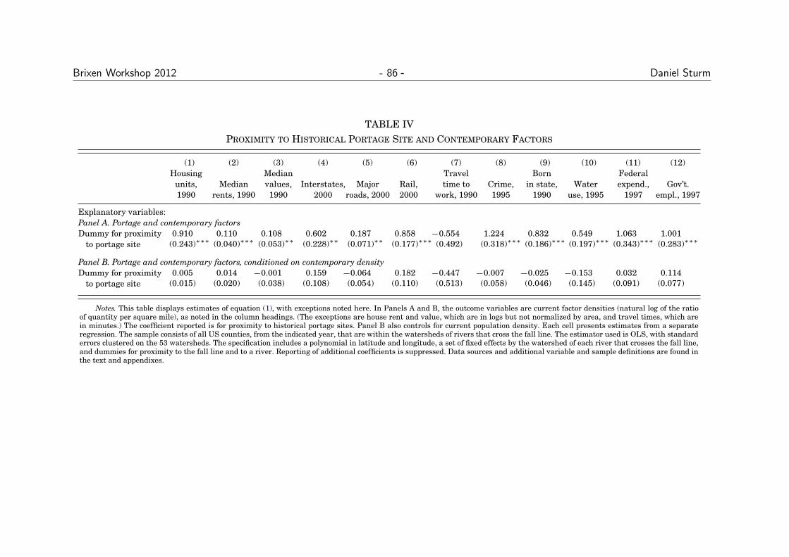
Brixen Workshop 2012 - 86 - Daniel Sturm630
QU
AR
TE
RL
YJ
OU
RN
AL
OF
EC
ON
OM
ICS
TABLE IV
PROXIMITY TO HISTORICAL PORTAGE SITE AND CONTEMPORARY FACTORS
(1) (2) (3) (4) (5) (6) (7) (8) (9) (10) (11) (12)Housing
units,1990
Medianrents, 1990
Medianvalues,1990
Interstates,2000
Majorroads, 2000
Rail,2000
Traveltime to
work, 1990Crime,1995
Bornin state,
1990Water
use, 1995
Federalexpend.,
1997Gov’t.
empl., 1997
Explanatory variables:Panel A. Portage and contemporary factorsDummy for proximity
to portage site0.910 0.110 0.108 0.602 0.187 0.858 −0.554 1.224 0.832 0.549 1.063 1.001
(0.243)∗∗∗ (0.040)∗∗∗ (0.053)∗∗ (0.228)∗∗ (0.071)∗∗ (0.177)∗∗∗ (0.492) (0.318)∗∗∗ (0.186)∗∗∗ (0.197)∗∗∗ (0.343)∗∗∗ (0.283)∗∗∗
Panel B. Portage and contemporary factors, conditioned on contemporary densityDummy for proximity
to portage site0.005 0.014 −0.001 0.159 −0.064 0.182 −0.447 −0.007 −0.025 −0.153 0.032 0.114
(0.015) (0.020) (0.038) (0.108) (0.054) (0.110) (0.513) (0.058) (0.046) (0.145) (0.091) (0.077)
Notes. This table displays estimates of equation (1), with exceptions noted here. In Panels A and B, the outcome variables are current factor densities (natural log of the ratioof quantity per square mile), as noted in the column headings. (The exceptions are house rent and value, which are in logs but not normalized by area, and travel times, which arein minutes.) The coefficient reported is for proximity to historical portage sites. Panel B also controls for current population density. Each cell presents estimates from a separateregression. The sample consists of all US counties, from the indicated year, that are within the watersheds of rivers that cross the fall line. The estimator used is OLS, with standarderrors clustered on the 53 watersheds. The specification includes a polynomial in latitude and longitude, a set of fixed effects by the watershed of each river that crosses the fall line,and dummies for proximity to the fall line and to a river. Reporting of additional coefficients is suppressed. Data sources and additional variable and sample definitions are found inthe text and appendixes.
at SWETS - Trusted Agent Gateway - OUP on September 16, 2012 http://qje.oxfordjournals.org/ Downloaded from

Brixen Workshop 2012 - 87 - Daniel Sturm
6.5 Conclusion
• Bleakley and Lin (2012) show that a long irrelevant naturaladvantage – portage – is clearly reflected in the density ofcontemporary economic activity.
• They argue that portage has simply helped to select one of manypossible equilibria for an agglomeration.
• Historical accidents therefore have profound long-run consequencesin a world of path-dependence.

Brixen Workshop 2012 - 88 - Daniel Sturm
• The results nevertheless also leave a number of open questions:
– What is the critical level of economic activity that a place needsto achieve to become self-sustaining?
– There are plenty of abandoned gold-rush cities in the US thatdied after the local gold-mines closed.
– Furthermore, the paper has little to say about the potential roleor effectiveness of policy in shaping spatial equilibria.

Brixen Workshop 2012 - 89 - Daniel Sturm
7 Outlook for future research
•While research in this area has produced a number of interestinginsights over the last years, there are still plenty of open questions.
• Let me highlight three areas in which our understanding is stillparticularly incomplete:
– How general are multiple spatial equilibria? Which industries areparticularly prone to multiple equilibria?
– Can economic policy play a meaningful role in shaping thespatial distribution of economic policy?

Brixen Workshop 2012 - 90 - Daniel Sturm
– Finally what are the welfare consequences of spatial equilibria?If the natural advantage of portage sites has evaporated, shouldcities ideally be located elsewhere?

Brixen Workshop 2012 - 91 - Daniel Sturm
8 Bibliography
Bleakley, Hoyt and Jeffrey Lin (2012) “Portage and PathDependence,” Quarterly Journal of Economics, 127(2), 587-644.
Brakman, Steven, Harry Garretsen, and Marc Schramm (2004)“Bombing of German Cities during WWII and its Impact on CityGrowth,” Journal of Economic Geography, 4(2), 201218.
Davis, Donald and David Weinstein (2002) “Bones, Bombs, andBreak Points: The Geography of Economic Activity,” AmericanEconomic Review, 92(5),1269-1289.

Brixen Workshop 2012 - 92 - Daniel Sturm
Davis, Donald and David Weinstein (2008) “A Search for MultipleEquilibria in Urban Industrial Structure,” Journal of Regional Science48(1), 29-65.
Fujita, Masahisa, Paul Krugman, and Anthony J. Venables (1999)The Spatial Economy: Cities, Regions and International Trade,Cambridge: MIT Press.
Krugman, Paul (1979) “Increasing Returns, MonopolisticCompetition, and International Trade,” Journal of InternationalEconomics, 9(4), 469-479.
Krugman, Paul (1991) “Increasing Returns and EconomicGeography,” Journal of Political Economy, 99(3), 483-499.

Brixen Workshop 2012 - 93 - Daniel Sturm
Miguel, Ted and Gerard Roland (2011) “The Long-run Impact ofBombing Vietnam,” Journal of Development Economics, 96(1), 1-15.
Redding, Steve, Daniel Sturm and Nikolaus Wolf (2011) “History andIndustry Location: Evidence from German Airports,” Review ofEconomics and Statistics, 93(3), 814-831.