Bridge System with Precast Concrete Double-T Girder and External Unbonded Post-tensioning

Bridge System with Precast Concrete Double-T Girder and External Unbonded Post-tensioning

by

Yang Eileen Li

A thesis submitted in conformity with the requirements for the degree of Master of Applied Science

Graduate Department of Civil Engineering University of Toronto

© Copyright by Yang Eileen Li (2010)

Bridge System with Precast Concrete Double-T Girder and External Unbonded Post-tensioning

Yang Eileen Li Master of Applied Science Graduate Department of Civil Engineering University of Toronto 2010

Abstract

This thesis compares the consumption of primary superstructure material in a

conventional single span CPCI system with those of double-T alternatives. The CPCI

system is currently the preferred bridge type for short and medium spans in Canada, despite

its relatively inefficient use of materials due to imperfect live load sharing among multiple

parallel girders. The double-T alternatives utilize slender double-T cross-sections, fully

precast segments, and post-tensioning in both longitudinal and transverse direction.

The economy of the CPCI and double-T systems is compared within the framework of

four sample designs. The results indicate that the double-T systems are in general more

efficient than the CPCI system and have the potential to achieve better economy.

ii

Acknowledgements

This project is partially funded by the National Science and Engineering Research

Council of Canada.

I would like to thank Professor Gauvreau without whom this work would not have been

possible. Professor Gauvreau has given me invaluable guidance and encouragement not only

during the course of this thesis, but throughout my years at the University of Toronto.

I would also like to thank Hatch Mott MacDonald for their financial contribution to this

project. The technical and personal support from Philip Murray and Biljana Rajlic of the

bridge group is deeply appreciated.

Thanks to my research colleagues for offering their help and insight to this thesis: Davis

Doan, Negar Elhamikhorasani, Kris Mermigas, Sandy Poon and Jason Salonga.

Finally, I would like to thank my parents for their patience and care throughout my

graduate studies.

iii

iv

Table of Contents Abstract ii

Acknowledgement iii

Table of Contents iv

List of Figures viii

List of Tables xi

List of Symbols xiii

Chapter 1: Introduction 1

1.1. Motivation 1

1.2. The Double-T Concept 4

1.2.1. Cross-Section 4

1.2.2. Prestressing Concept 5

1.2.3. Construction 6

1.3. Geometrical Requirements for Sample Designs 7

1.4. Objective and Scope 7

Chapter 2: Double-T Base Concept 9

2.1. Brief Description of Design 9

2.2. Material Properties 12

2.3. Design Criteria 13

2.3.1. Serviceability Limit States 14

2.3.2. Ultimate Limit States 15

2.4. Loads, Load Combinations and Post-tensioning Parameters 15

2.4.1. Dead Load and Superimposed Dead Load 15

v

2.4.2. Live Load 16

2.4.3. Post-tensioning Parameters 17

2.4.4. Load Factors and Load Combinations 18

2.5. Transverse System Design 21

2.5.1. Load Effects 21

2.5.2. Design Approach 21

2.5.3. Final Design 23

2.6. Torsion and Live Load Distribution 24

2.6.1. Analytical Approach 24

2.6.1.1. Torsion 24

2.6.1.2. Parametric Study on Torsion 27

2.6.1.3. Live Load Distribution based on Analytical Approach 29

2.6.2. Grillage Model Analysis 31

2.7. Longitudinal Flexure 34

2.7.1. Unbonded Tendons 34

2.7.2. Prestress Losses 35

2.7.3. Flexural Response under SLS 40

2.7.4. Flexural Response under ULS 42

2.7.5. Shear 46

2.8. Local Forces 47

2.8.1. Anchorage Zone 47

2.8.2. Deviation 49

2.9. Construction 50

2.9.1. Precast Segment Design 50

2.9.2. Precast Concrete Forming 52

2.9.3. Girder Erection 52

2.10. Final Remarks 53

Chapter 3: Double-T Alternative Concept I 54

3.1. Fibre-Reinforced Polymer (FRP) Reinforcing Systems 55





3.4.2. Fatigue Limit States 59

vi


3.5. Load Combinations and Associated Prestress Parameters 62


3.6.1. Prestress Losses 63




3.7. Shear Design 68


Chapter 4: Double-T Alternative Concept II 70












Chapter 5: Slab-on-Girder Bridge System with CPCI Girders 79

5.1. Introduction 79



5.4. Live Load Distribution 82

5.4.1. AASHTO Standard 83

5.4.2. AASHTO LRFD Specifications 84

5.4.3. Canadian Highway Bridge Design Code 85

5.5. Deck Slab Design 88

5.5.1. Arching Action 88

5.5.2. Empirical Design Method from CHBDC 89

5.6. Construction 90

vii

5.6.1. CPCI Girder Fabrication 90

5.6.2. Erection 91

Chapter 6: Evaluation of the Double-T and CPCI systems 92

6.1. Comparison of Double-T Concepts 92

6.2. Comparison of Double-T Systems with CPCI Slab-on-Girder System 96

6.2.1. Live Load Distribution 96

6.2.2. Design Load 97

6.2.3. Deck Slab Design 98

6.3. Material Consumption 99

6.3.1. Concrete 99

6.3.2. Prestressing Steel 100

6.3.3. Reinforcing Steel 101

6.3.4. CFRP Reinforcing System 101

6.4. Cost Comparison 102

6.4.1. Cost Comparison of Double-T Systems 102

6.4.2. Cost Comparison between Double-T and CPCI Systems 103

Chapter 7: Conclusion 107

References 109

Appendices 113

Appendix A: Double-T Concepts Sample Calculations and Design Drawings 113

A.1. Sample Calculations 114

A.2. Design Drawings 128

Appendix B: CPCI Slab-on-Girder System Sample Calculations and Design Drawings 138

B.1. Sample Calculations 139

B.2. Design Drawings 150

Appendix C: Grillage Model Input File from SAP 152

viii

List of Figures 1.1. CPCI slab-on-girder system (CPCI, 2009) 2

1.2. Cross-section of CPCI girders (adapted from Pre-Con, 2004) 2

1.3. Idealized model of load distribution in a slab-on-girder system 3

1.4. Web thickness of a double-T girder 5

1.5. Double-T girder cross-section 5

1.6. Matching casting of box girder segments (adapted from Interactive Design Systems, 2009) 6

1.7. Roadway cross-section 7

2.1. Sample design of double-T base concept 10

2.2. Longitudinal prestressing design of double-T concept 11

2.3. Transverse prestressing design of double-T concept 12

2.4. Material stress-strain relationships 13

2.5. Schematic diagram of stress in unbonded tendon as a function of member curvature 14

2.6. Dead load and superimposed dead load for sample design 15

2.7. CL-W and CL-625-ONT live load models (adapted from CSA, 2006a) 16

2.8. Design lane layout 16

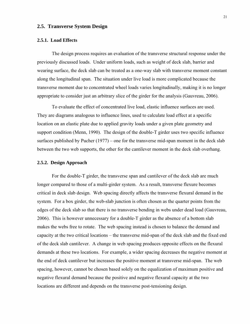
2.9. Transverse tendon profile 22

2.10. Integrated process of transverse flexural design 22

2.11. Flexural demand and capacity of transverse system as a function of web spacing 23

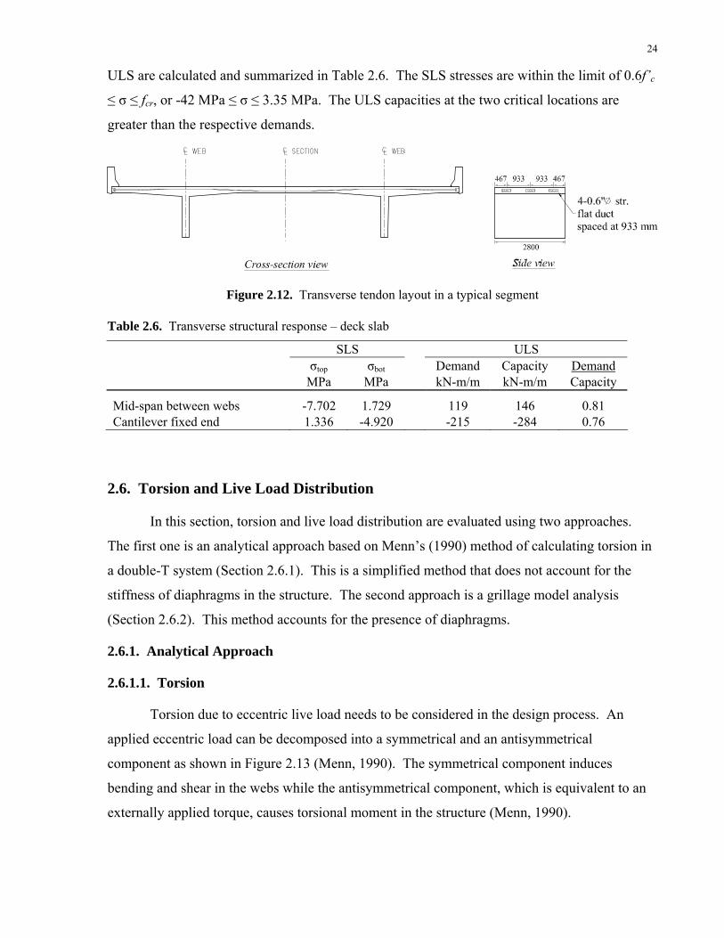
2.12. Transverse tendon layout in a typical segment 24

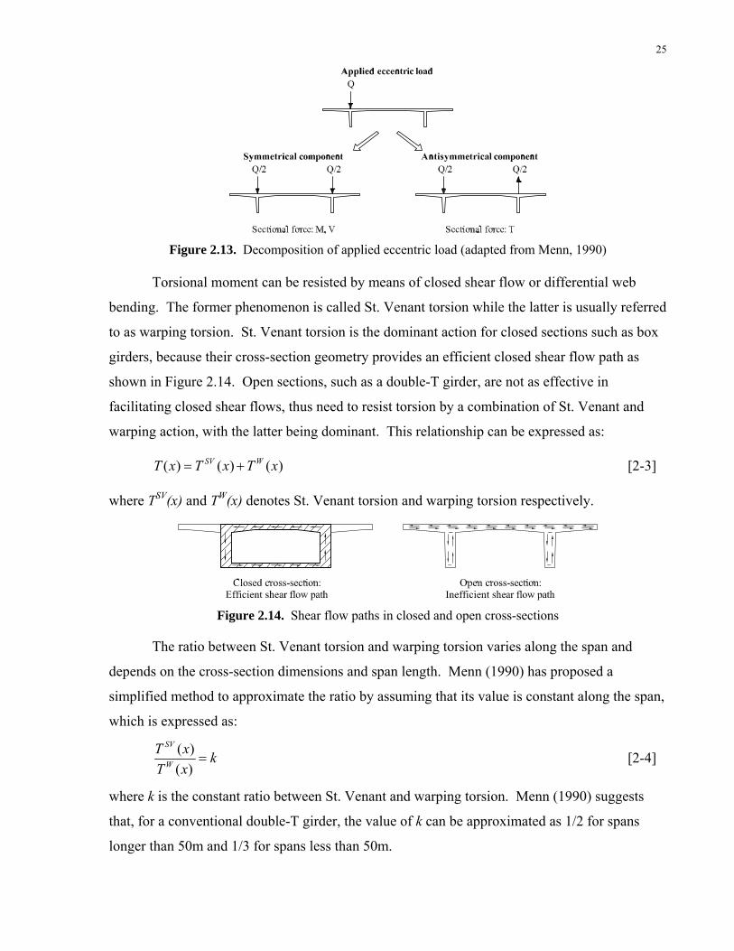
2.13. Decomposition of applied eccentric load (adapted from Menn, 1990) 25

2.14. Shear flow paths in closed and open cross-sections 25

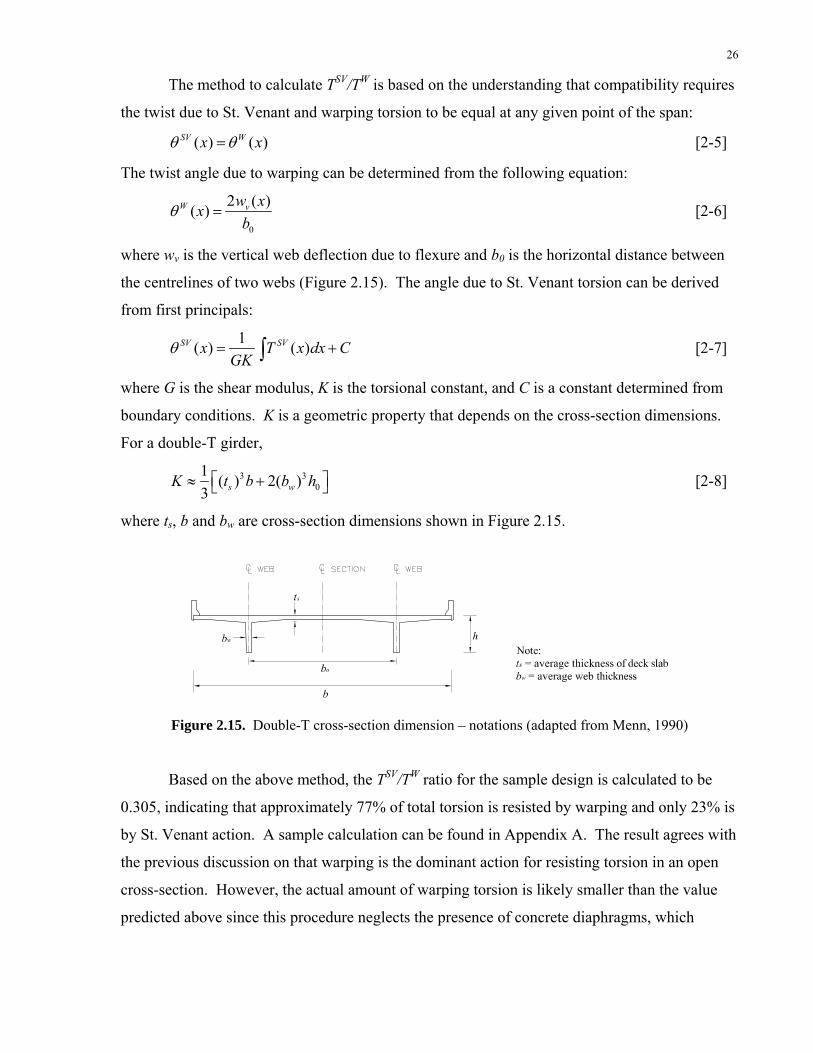
2.15. Double-T cross-section dimension – notations (adapted from Menn, 1990) 26

2.16. Differential web bending due to warping torsion (adapted from Menn, 1990) 27

2.17. Torsion distribution with varying web thickness and span length 28

2.18. Load cases for evaluating live load distribution 30

2.19. Maximum moment per web as a function of k 31

2.20. Grillage model of double-T system 32

2.21. Position of truck wheel load for Load Case 2 and 3 32

ix

2.22. Example of equivalent load used in applying wheel load 32

2.23. Member forces and deformation from grillage model 33

2.24. Compatibility relationship for bonded and unbonded tendons under ultimate limit states 34

2.25. Parameters in determining creep coefficient φ (Menn, 1990) 38

2.26. Summary of prestress losses in sample design 39

2.27. Concrete stress under SLS 41

2.28. Concrete stress sensitivity to level of prestress 41

2.29. Iterative procedure for calculating post-tensioning force in unbonded tendons under ULS 43

2.30. Concrete stress under load combination ULS 1A and 1B 44

2.31. Moment and girder deformation under load combination ULS 1D 44

2.32. Moment diagram under load combination ULS 1C 45

2.33. Negative flexural capacity of girder under load combination ULS 1C 45

2.34. Shear design for the base concept 47

2.35. Equilibrium of anchorage zone 48

2.36. Anchorage location of external tendons 48

2.37. Anchorage zone truss model 49

2.38. Deviation truss model 50

2.39. Segment layout 50

2.40. Segment geometry 51

2.41. Schematic illustration of formwork for an interior segment 52

2.42. Erection girder with overhanging platform 53

3.1. Comparison of cross-sections of double-T base concept and alternative concept I 54

3.2. A beam strengthened with CFRP flexure plates and L-shaped shear plates (Sika, 2009) 55

3.3. Design of alternative concept I 57

3.4. Typical CFRP and mild-steel stress-strain relationship (adapted from Teng, 2002) 59

3.5. FRP related failure modes of members reinforced with externally bonded FRP system

(adapted from ACI, 2008 and Teng, 2002)

61

3.6. Prestress losses for alternative concept I 64


3.8. Moment diagrams under ULS load combinations 65

3.9. Concrete stress under negative-flexure-critical ULS load combinations 66

3.10. System behaviour under ULS 1D 67

3.11. Schematic diagrams of moments under load combination ULS 1D and FLS 1 68

3.12. Shear design for alternative concept 69

x

4.1. Comparison of cross-section between double-T base concept and alternative concept II 70

4.2. Design of alternative concept II 72


4.4. External load and internal forces under load combinations SLS 1B and SLS 1D 75

4.5. Moment diagrams under ULS load combinations 76

4.6. Concrete stress under negative-flexure-critical ULS load combinations 76

4.7. System behaviour under ULS 1D 77

5.1. Standardized I sections (adapted from Pre-Con, 2004 and FHWA, 2009) 80

5.2. Sample design of the Slab-on-CPCI-girder system 81

5.3. Pre-tension strand layout (adapted from MTO, 2002) 81

5.4. Load distribution in an idealized beam-on-girder system

(adapted from Hassanain, 1998)

83

5.5. Fm for internal girders in a slab-on-girder bridge system under ULS and SLS (CSA, 2006b) 86

5.6. Arching action in deck slab (adapted from Batchelor, 1987) 89

5.7. Punching shear failure mode (adapted from Batchelor, 1987) 89

5.8. Typical deck slab design based on CHBDC’s empirical method – cross-section view 90

5.9. CPCI girder fabrication (photos by P. Gauvreau) 91

5.10. Typical construction sequence for the superstructure of a slab-on-girder bridge

(adapted from WSDOT, 2008)

91

xi

List of Tables 1.1. Examples of existing post-tensioned double or triple-T girder bridges 4

2.1. Material property for double-T base concept sample design 12

2.2. SLS stress limits (adapted from CSA, 2006a) 15

2.3. Post-tensioning parameters 17

2.4. Load factors (CSA, 2006a) 18

2.5. Load combinations for the double-T sample design 19

2.6. Transverse structural response – deck slab 24

2.7. Variables considered in parametric study for torsion 28

2.8. Live load distribution under applied eccentric load – analytical approach 29

2.9. Live load distribution – analytical approach 30

2.10. Comparison of analytical approach and grillage model results 34

2.11. Anchor set loss with varying l 36

2.12. Loss due to creep and shrinkage and related parameter 38

2.13. Stress in post-tensioning steel under SLS 40

2.14. Summary of flexural response under ULS 46

2.15. Anchorage zone reinforcing steel 49

2.16. Deviation reinforcing steel 50

3.1. Material properties 58

3.2. SLS stress limits 59

3.3. Fatigue limit states load combination 62

3.4. Level of prestress used in SLS load combinations 63

4.1. Material properties 72

4.2. SLS stress limits 73

5.1. Material properties for slab-on-CPCI-girder sample design 82

5.2. Summary of live load distribution equations 88

xii

6.1. Comparison of double-T systems 95

6.2. Live load distribution comparison 96

6.3. Maximum moment intensity due to DL, SDL, and LL 98

6.4. Concrete consumption 99

6.5. Prestressing steel consumption 100

6.6. Reinforcing steel consumption 101

6.7. CFRP reinforcing system (Data provided by Sika, Canada) 101

6.8. Unit cost of structural reinforcing systems 102

6.9. Cost comparison of double-T systems 102

6.10. Qualitative cost comparison of the double-T and CPCI systems 104

6.11. Cost of precast concrete and cast-in-place deck slab 105

6.12. Cost comparison between the CPCI system and double-T alternative concept II 106

xiii

List of Symbols A Area of concrete cross-section

As Area of reinforcing steel

Astrand Area of each prestresing strand

ANC Prestress loss due to anchor set

b Deck slab width (Figure 2.9)

b0 Width between centrelines of the two webs in a double-T cross-section (Figure 2.9)

bw Average web thickness (Figure 2.9)

Cf Factor for lane width correction factor, which is used in calculating live load distribution

based on CHBDC

D D value in AASHTO equation for calcuating live load distribution among girders

DF Distribution factor characterizing transverse live load distribution in a bridge system

e(x) Distance from centroid of the gross uncracked concrete section to the centroid of

prestressing steel

Ec Modulus of Elasticity of concrete

Ef Modulus of Elasticity of FRP

Ep Modulus of Elasticity of prestressing steel

Es Modulus of Elasticity of reinforcing steel

f'c Specified compressive strength of concrete

fo Jacking stress of post-tensioning tendon

fpy Yield strength of prestressing steel

fpu Specified tensile strength of prestressing steel

fy Yield strength of reinforcing steel

F Width dimension that characterizes the load distribution for a bridge

Fm

FR Prestress loss due to friction

G Shear modulus

k Ratio between St. Venant and warping torsion, assumed to be constant along along the

span

K Torsional constant

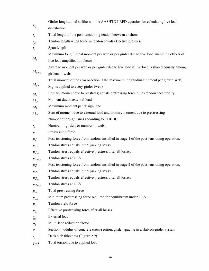
xiv

Kg Girder longitudinal stiffness in the AASHTO LRFD equation for calculating live load

distribution

lp Total length of the post-tensioning tendon between anchors

lp0 Tendon length when force in tendon equals effective prestress

L Span length

Mg Maximum longitudinal moment per web or per girder due to live load, including effects of

live load amplification factor

Mg,avg Average moment per web or per girder due to live load if live load is shared equally among

girders or webs

Mg,tot Total moment of the cross-section if the maximum longitudinal moment per girder (web),

Mg, is applied to every girder (web)

Mp Primary moment due to prestress; equals pretressing force times tendon eccentricity

MQ Moment due to external load

MT Maximum moment per design lane

Mtot Sum of moment due to external load and primary moment due to prestressing

n Number of design lanes according to CHBDC

N Number of girders or number of webs

P Prestressing force

P1 Post-tensioning force from tendons installed in stage 1 of the post-tensioning operation.

P1i Tendon stress equals initial jacking stress.

P1∞ Tendon stress equals effective prestress after all losses.

P1ULS Tendon stress at ULS


P2i Tendon stress equals initial jacking stress.

P2∞ Tendon stress equals effective prestress after all losses.

P2ULS Tendon stress at ULS

Ptot Total prestressing force

Pmin Minimum prestressing force required for equilibrium under ULS

Py Tendon yield force

P∞ Effective prestressing force after all losses

Qf External load

RL Multi-lane reduction factor

S Section modulus of concrete cross-section; girder spacing in a slab-on-girder system

ts Deck slab thickness (Figure 2.9)

T(x) Total torsion due to applied load

xv

TSV(x) St. Venant torsion

TW(x) Warping torsion

wv Vertical girder deflection due to longitudinal flexure

W Axle load of truck load model

We Width of a design lane

α(x) Tendon angle change from jacking end to location x

αD Load factor for dead load

ΔlPD Tendon elongation due to deformation

ΔlPF Tendon elongation due to tendon force

Δset Change in length of post-tensioning tendon due to anchorage slip

Δεp Change in strain in prestressing steel due to deformation

εcp Concrete strain at the level of prestressing steel

εcs(t) Concrete shrinkage strain

εct Concrete tensile stress

εfd FRP debonding strain

εfu FRP ultimate strain

θSV(x) Twist angle due to St. Venant torsion

θW(x) Twist angle due to warping torsion

μ Friction coefficient; aging coefficient of concrete; factor for lane width correction factor,

which is used in calculating live load distribution based on CHBDC

ρ Reinforcement ratio

σc0(x) Concrete stress at the level of prestressing steel due to initial load

σc,bot Concrete stress in section's bottom fibre

σc,top Concrete stress in section's top fibre

φ Curvature

φ(t) Creep coefficient of concrete

Chapter 1 Introduction

This thesis compares the consumption of primary superstructure material (concrete,

prestressing steel and other reinforcements) in a conventional single span slab-on-girder system

with those of double-T alternatives. The slab-on-girder system addressed in this thesis consists

of a series of parallel CPCI (Canadian Precast Prestressed Concrete Institute) girders, which are

standardized I sections used in Canada, with a cast-in-place deck slab. A sample design of the

CPCI girder bridge will be developed with standard methods used in the industry. The double-T

concepts involve the use of slender cross-section, fully precast concrete, and external unbonded

post-tensioning. Three double-T concepts will be developed and validated in this thesis with

sample designs. The three concepts are:

1. Base concept: a double-T system with pure external unbonded post-tensioning;

2. Alternative concept I: a double-T system with a blend of external unbonded post-tensioning

and external carbon-fibre-reinforced polymer (CFRP) laminate reinforcements;

3. Alternative concept II: a double-T system with a blend of external unbonded post-

tensioning and internal bonded unstressed tendons.

This thesis will compare the material consumption and cost of the slab-on-CPCI-girder system

with the double-T systems based on their design examples.

1.1. Motivation

Long span bridges with their grand appearance often attract most of the public attention.

Records for the longest spans in the world are constantly being challenged or broken as a

reflection of people’s fascination with long spans and the extensive technological interest that

follows it. In the bridge industry, however, the largest section comprises short and medium

spans, ranging approximately from 20 m to 45 m. These may be single span bridges, or parts of

a longer multi-span structure. Given the large market share of this type of project, it follows

that short-to-medium spans are of great economical importance to the society and deserve as

1

2

much if not more attention than long spans (Kulka and Lin, 1984). For instance, any reduction

in material consumption of short-to-medium span structures will be magnified by the large

number of their applications and result in substantial overall economical improvement.

In most parts of Canada, the preferred structural system for spans of up to about 45 m is

the CPCI slab-on-girder system, which consists of multiple parallel precast, pre-tensioned

concrete CPCI girders with a cast-in-place concrete deck slab (Figure 1.1). CPCI girders,

shown in Figure 1.2, are precast I sections commonly used in Canada. The CPCI slab-on-girder

system has become very much standardized, making its design and construction relatively

straightforward. Consequently, when facing this type of project, owners and designers are often

reluctant to consider alternatives that may be more efficient and economical.

Figure 1.1. CPCI slab-on-girder system Figure 1.2. Cross-section of CPCI girders (CPCI, 2009) (adapted from Pre-Con, 2004)

Although the cost of the CPCI system is often considered to be acceptable by owners,

this system actually makes relatively inefficient use of materials. One primary source of

inefficiency in this type of bridge comes from the imperfect sharing of live load among multiple

parallel girders due to transverse flexibility of the deck slab. An idealized example with stick

models is illustrated in Figure 1.3. As shown in the figure, if the deck slab is infinitely stiff, it

rotates under applied eccentric load and engages multiple girders in resisting the load. On the

other hand, if the deck slab is infinitely flexible, it bends under the applied load and only

engages the girder directly below or adjacent to the load. The CPCI slab-on-girder system is in

between the two extreme cases but close to the case with the flexible deck slab. This inefficient

load distribution requires every girder in the system to be designed for relatively high loading,

which, in combination with the relatively large number of girders in a CPCI system, results in an

unnecessarily high design load for the overall structure. The inefficient live load distribution in

the CPCI slab-on-girder system is qualitatively discussed in Chapter 5.

3

Figure 1.3. Idealized model of load distribution in a slab-on-girder system

Another source of inefficiency associated with live load distribution comes from the

actual method of calculating it. Much research has been done in modeling live load distribution

in a slab-on-girder system using grillage, semi-continuum or finite element methods (CSA

2006b.). The results from these analyses are used to formulate design equations in standards

and codes. However, these equations are often simplified from the real situation to include only

a limited number of variables. They usually determine the maximum amount of load distributed

to a girder under the most unfavourable conditions. The design equations for live load

distribution from AASHTO Standards, AASHO LRFD Specifications and CHBDC, will be

examined in Chapter 5.

In addition to the structural inefficiencies associated with live load distribution, the

construction of a CPCI girder bridge can also be problematic due to its cast-in-place deck slab.

The casting of the deck slab is an inconvenient and time-consuming process which involves

installing formwork, placing the deck slab reinforcements, casting and curing concrete, and

removing formwork if necessary. The non-prestressed deck slab is also a source of durability

problems due to slab’s tendency to crack. Once crack forms, salts and other chemical agents

penetrate the concrete and induce corrosion in the reinforcing steel.

Recognizing the large demand in short and medium span bridges and the inefficiency of

current solution – the CPCI slab-on-girder system, this thesis aims to develop a new structural

system based on a double-T cross-section. The new double-T concept will be developed with

the specific intent of maximizing the efficient use of concrete and prestressing steel, as well as

simplifying the construction process. The material consumption will then be compared to the

CPCI system to provide a qualitative measure of the greater efficiency of the double-T system.

4

1.2. The Double-T Concept

1.2.1. Cross-Section

Recognizing the inherent inefficiency of live load distribution in a slab-on-girder system,

the new concept is based on a two-web double-T cross-section. Double-T girders, which are not

common in North America, have seen most of their use in Europe. Post-tensioned double or

triple-T girder bridges, as shown in Table 1.1, have traditionally incorporated thick webs to

accommodate internal post-tensioning tendons. The combination of cover requirements and

clearance requirements for construction (i.e. distance between tendon ducts to allow proper

placement and vibration of concrete) generally results in a minimum web thickness of

approximately 440 mm (Figure 1.4 (a)).

Table 1.1. Examples of existing post-tensioned double or triple-T girder bridges

Bridge Cross-section Web thickness Notes (Reference)

le viaduc d'Orbe, Switzerland

1050 mm (Departement des Travaux Publics du Canton de Vaud, 1989)

Weinlandbrucke Andelfingen 500 mm

Cross-section is variable along span. The triple-T section shown is for the region close to mid-span. For regions close to support, bottom slabs are added, creating a twin-box girder. (Stussi, 1958)

Isarbrucke Munchen 700 mm (Leonhardt, 1979)

Rheinbrucke Emmerich Vorlandbrucken

1150 mm (Leonhardt, 1979)

The new double-T concept is developed with the specific intention to minimize the

amount of concrete in the system. Hence the relatively thick webs in the traditional double-T

girder need to be modified. In the new concept, web thickness is reduced by removing the

internal tendons, and replacing them with external unbonded tendons (Figure 2.7(b)). By doing

so, the web thickness can be reduced to at least 300 mm and possibly lower because web

thickness is no longer governed by detailing requirements, but rather by stress.

5

(a) (b)

Figure 1.4. Web thickness of a double-T girder: (a) with internal tendons (adapted from Menn, 1990); (b) with external tendons

The double-T cross-section that will be used in this thesis is illustrated in Figure 1.5. It

consists of a 225 mm thick top slab and two slender webs. The webs have an average thickness

of 300 mm, and are tapered to facilitate the forming process. The thickness of 300 mm is

consistent with the standard practice of box girder cross-sections with similar span and girder

depth (ASBI, 2008). The deck width is governed by the roadway cross-section, which is

presented in the section of Geometrical Requirements for Sample Designs (Section 1.3). The

overall depth of the cross-section is chosen to be 2 m based on the span length (36.6m, see

Section 1.3) and typical span-to-depth ratios, which range from 17:1 to 22:1 for constant-depth

girders (Menn, 1990). The web spacing is chosen to be 7.9 m based on an optimization process

of the girder’s transverse flexural behaviour. Details of the analysis can be found in Section 2.5.

Figure 1.5. Double-T girder cross-section

1.2.2. Prestressing Concept

The double-T concept involves post-tensioning in both the longitudinal and transverse

directions. Longitudinally, the system is post-tensioned with external unbonded tendons.

Transversely, the deck slab is post-tensioned with internal flat-duct tendons. Transverse post-

6

tensioning serves primarily two purposes: 1) providing transverse bending capacity to the deck

slab; 2) controlling crack in the deck slab thus enhancing the system’s durability. Details of

longitudinal and transverse post-tensioning design will be presented in subsequent chapters.

1.2.3. Construction

The new double-T concept employs precast segmental construction technology which

allows bridge to be built rapidly with minimal impact to traffic. Segments will be fabricated of-

site with the method of match-casting, which produces custom-fitted joints by casting a new

segment against a dry mating segment (Figure 1.6). Segments produced by such method can be

erected on site speedily without the need of cast-in-place concrete or grout (Gauvreau, 2006).

New segment

Core form

Match-cast

Completed

mate segment

segment

Figure 1.6. Match casting of box girder segments (adapted from Interactive Design Systems, 2009)

The precast segmental method is most often used for large projects. This is because the

initial cost of the segmental method, which is associated with manufacturing the forming

equipment, is usually high and hard to be justified if a large number of segments is not needed.

The most expensive part of the forming equipment is the core form (shown in Figure 1.6). It

can slide in and out during the match-casting of box girder segments, thus allowing the entire

rebar cage to be prefabricated. The decoupling of rebar fabrication and the actual casting

process can simplify the casting procedures and improve both casting speed and quality. The

forming of double-T girder segments, however, does not require such a core form due to the

absence of a bottom slab. The rebar cages can be prefabricated and used during casting with

formwork simply made of plywood which is relatively low in cost. Without the high initial cost

of forming equipment, the segmental construction method becomes a feasible and economical

choice for short-to-medium span double-T systems.

7

1.3. Geometrical Requirements for Sample Designs

The CPCI slab-on-girder system and the three double-T concepts will be evaluated based

on their sample designs. To form a consistent basis of comparison, all four sample designs will

be developed under the same geometrical requirements. These requirements are representative

of the general highway bridge design conditions in Ontario. First, the bridge needs to cross a

distance of 36.6 m with one simply-supported span. Second, the roadway cross-section needs to

accommodate three traffic lanes, each 3.6 m wide, and two shoulder lanes, each 1.2 m wide

(Figure 1.7). The travelled and the total deck width are 13.2 m and 13.8 m, respectively. The

road deck wearing surface is assumed to be 90 mm in thickness.

Figure 1.7. Roadway cross-section

1.4. Objective and Scope

The objective of this thesis is to compare the consumption of primary superstructure

materials (concrete, prestressing steel, and additional reinforcements) in a conventional single

span CPCI system with those of double-T alternative systems. A total of four systems are

investigated in this thesis:

1. Double-T base concept: a double-T system with pure external unbonded post-tensioning;

2. Double-T alternative concept I: a double-T system with a blend of external unbonded post-

tensioning and external carbon-fibre-reinforced polymer (CFRP) laminate reinforcements;

3. Double-T alternative concept II: a double-T system with a blend of external unbonded post-

tensioning and internal bonded unstressed tendons

4. CPCI slab-on-girder system

A sample design is produced for each of the four systems above under the general highway

bridge design conditions in Ontario.

Chapters 2 to 4 describe and discuss the three double-T concepts within the framework

of three sample designs. Chapter 2 presents a comprehensive review on the design of the

double-T base concept, including the system’s transverse flexure, torsion, live load distribution,

8

longitudinal flexure and shear, anchorage and deviation regions, as well as construction.

Chapters 3 and 4 present the design of double-T alternative concept I and II. These two

alternative concepts are modified versions of the base concept and share a number of same traits

with the base concept, such as transverse flexure, torsion, live load distribution and local designs.

As a result, Chapters 3 and 4 only focus on the differences between the alternative concepts and

the base concept, which is primarily longitudinal flexure.

Chapter 5 is dedicated to the CPCI slab-on-girder system. A sample design is presented.

Two important aspects in this type of system, live load distribution and deck slab design, are

also discussed.

Chapter 6 compares the four systems based on the sample designs developed. First, the

three double-T concepts are evaluated on their differences in flexural behaviour. Next, the

CPCI slab-on-girder system is compared with the double-T systems in terms of structural

efficiency, such as live load distribution. Finally, a comparison is made on the material

economy between the CPCI slab-on-girder system and the double-T systems.

The final chapter concludes the thesis by summarizing the important findings from the

development of the double-T systems, and the comparison between the systems’ material

economy.

Chapter 2 Double-T Base Concept

– Double-T System with Pure External Unbonded Post-Tensioning

This chapter describes the design of the double-T base concept, which is a double-T

system with pure external unbonded post-tensioning. The concept is presented within the

framework of a sample design, which is briefly described in Section 2.1. While most of details

regarding design procedures and analyses are presented in the later sections, it is helpful to

outline some of the main aspects the design and set up the framework at the beginning of the

chapter for a more clear understanding of the later discussions. Following the description of the

design, Section 2.2 and 2.3 outline the material properties and the design criteria. Section 2.4

describes the loadings and the associated factors and load combinations. Sections 2.5 to 2.6

examine the system’s transverse behaviour, torsion, and live load distribution, while Section 2.7

investigates the structural system’s global longitudinal response, such as longitudinal flexure

and shear. Local effects in the anchorage and deviation zone are analyzed in Section 2.8, while

Section 2.9 is dedicated to construction related subjects.

2.1. Brief Description of Design

The plan, elevation and cross-section of the base concept are shown in Figure 2.1. The

concrete cross-section and its features were already explained in Chapter 1 (Section 1.2.1).

Concrete details at the ends of the span are designed to accommodate expansion joints and post-

tensioning anchorages (Section 2.8). Two deviation diaphragms are provided along the span to

accommodate the deviation of the external unbonded tendons. For a complete set of drawings,

the reader can refer to Appendix A.

9

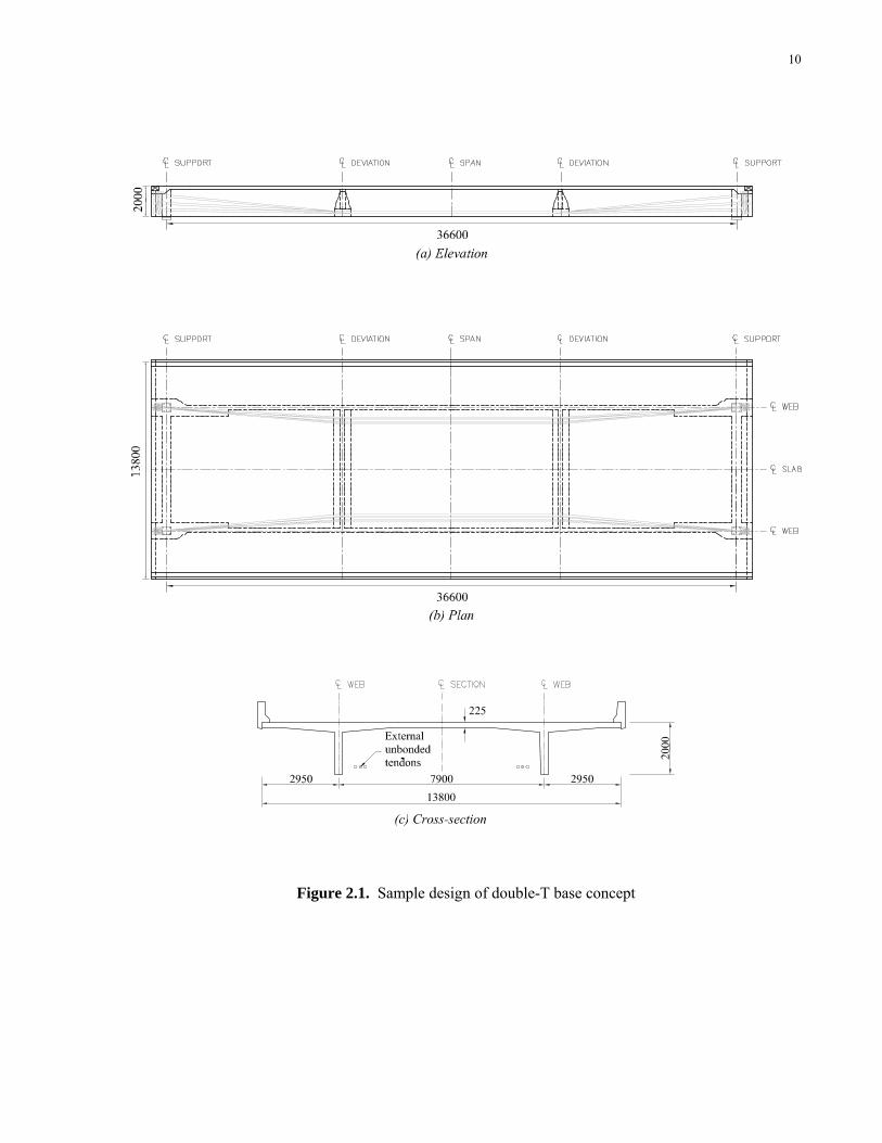
10

Figure 2.1. Sample design of double-T base concept

11

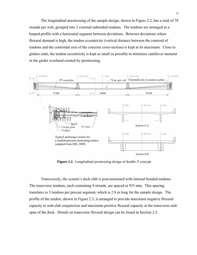
The longitudinal prestressing of the sample design, shown in Figure 2.2, has a total of 78

strands per web, grouped into 3 external unbonded tendons. The tendons are arranged in a

harped profile with a horizontal segment between deviations. Between deviations where

flexural demand is high, the tendon eccentricity (vertical distance between the centroid of

tendons and the centroidal axis of the concrete cross-section) is kept at its maximum. Close to

girders ends, the tendon eccentricity is kept as small as possible to minimize cantilever moment

in the girder overhand created by prestressing.

Typical anchorage system fora multistrand post-tensioning tendon(adapted from DSI, 2009)

Figure 2.2. Longitudinal prestressing design of double-T concept

Transversely, the system’s deck slab is post-tensioned with internal bonded tendons.

The transverse tendons, each containing 4 strands, are spaced at 933 mm. This spacing

translates to 3 tendons per precast segment, which is 2.8 m long for the sample design. The

profile of the tendon, shown in Figure 2.3, is arranged to provide maximum negative flexural

capacity at web-slab conjunction and maximum positive flexural capacity at the transverse mid-

span of the deck. Details on transverse flexural design can be found in Section 2.5.

12

Figure 2.3. Transverse prestressing design of double-T concept

2.2. Material Properties

The material properties assumed for the sample design are summarized in Table 2.1.

The design chooses to utilize concrete with a compressive strength of 70 MPa because

preliminary design indicates that 70 MPa is approximately the minimum strength required for

satisfactory structural response under SLS and ULS. Although the current standard practice in

Ontario is to use 50 MPa concrete, concrete with a compressive strength of 70 MPa or above has

become commercially available and has seen increased application in North America as a result

of the recent advancement in concrete technology (Choi et al, 2008).

Table 2.1. Material property for double-T base concept sample design

Material Strength Modulus of Elasticity

Concrete Specified compressive strength: 1.5( ' 6900)( / 2300)c c cE f γ= + f'c = 70 MPa Ec = 36 300 MPa Cracking strength: 0.4 ' 3.35MPacr cf f= = Reinforcement Yield strength: Es = 200 000 MPa fy = 400 MPa Prestressing steel Specified tensile strength: Ep = 200 000 MPa Size 15 fpu = 1860 MPa (Astrand = 140 mm2) Yield strength: fpy = 0.90fpu = 1674 MPa

13

The material stress-strain relationships assumed in the design are illustrated in Figure 2.4.

Concrete is assumed to behave linear-elastically up to 60% of f’c. Reinforcing steel and

prestressing steel’s stress-strain diagrams are approximated as bi-linear. The yield stress of

prestressing steel is assumed to be at approximately 90% fpu.

Figure 2.4. Material stress-strain relationships

2.3. Design Criteria

The Canadian Highway Bridge Design Code (CSA, 2006a) is used as the primary design

standard in this thesis. CHBDC is a limit-states code, under which bridge components need to

satisfy the requirements at three limit states – serviceability limit states (SLS), fatigue limit

states (FLS), and the ultimate limit states (ULS) (CSA, 2006a). The design of the double-T base

concept in this chapter focuses on the structural response under SLS and ULS. Fatigue is

associated with repeated stress cycles leading to crack or fracture in metals. According to

CHBDC, FLS needs to be checked for reinforcing bars and prestressing tendons in a concrete

structure. For the structural system under study, the primary longitudinal and transverse

reinforcements are post-tensioned prestressing steel, of which the stress range under SLS is very

small because concrete remains uncracked (Figure 2.5). Under FLS loading, the stress range

becomes more negligible as FLS imposes only one lane of live load. As a result, FLS is likely

not a governing limit state for the double-T base concept under study and thus not focused on in

the design. For double-T alternative concepts I and II which use a blend of post-tensioned and

non-post-tensioned reinforcements, FLS will be examined explicitly in Chapters 3 and 4.

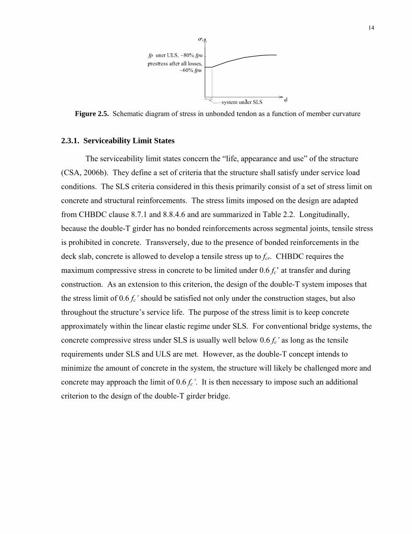
14

Figure 2.5. Schematic diagram of stress in unbonded tendon as a function of member curvature

2.3.1. Serviceability Limit States

The serviceability limit states concern the “life, appearance and use” of the structure

(CSA, 2006b). They define a set of criteria that the structure shall satisfy under service load

conditions. The SLS criteria considered in this thesis primarily consist of a set of stress limit on

concrete and structural reinforcements. The stress limits imposed on the design are adapted

from CHBDC clause 8.7.1 and 8.8.4.6 and are summarized in Table 2.2. Longitudinally,

because the double-T girder has no bonded reinforcements across segmental joints, tensile stress

is prohibited in concrete. Transversely, due to the presence of bonded reinforcements in the

deck slab, concrete is allowed to develop a tensile stress up to fcr. CHBDC requires the

maximum compressive stress in concrete to be limited under 0.6 fc’ at transfer and during

construction. As an extension to this criterion, the design of the double-T system imposes that

the stress limit of 0.6 fc’ should be satisfied not only under the construction stages, but also

throughout the structure’s service life. The purpose of the stress limit is to keep concrete

approximately within the linear elastic regime under SLS. For conventional bridge systems, the

concrete compressive stress under SLS is usually well below 0.6 fc’ as long as the tensile

requirements under SLS and ULS are met. However, as the double-T concept intends to

minimize the amount of concrete in the system, the structure will likely be challenged more and

concrete may approach the limit of 0.6 fc’. It is then necessary to impose such an additional

criterion to the design of the double-T girder bridge.

15

Table 2.2. SLS stress limits (adapted from CSA, 2006a)

Concrete (CHBDC clause 8.8.4.6) Tendon (CHBDC clause 8.7.1)

Tension At jacking ≤ 0.80 fpu Longitudinal ≤ 0 MPa Transverse ≤ fcr, 3.35 MPa

CHBDC requirements

Compression at transfer and during construction

≤ 0.6 f’c

Additional requirements

Compression at all other stages

≤ 0.6 f’c

2.3.2. Ultimate Limit States

The ultimate limit states are related to the structural safety of the bridge (CSA, 2006b).

Under ultimate limit states, the structure’s factored resistance should be greater than or equal to

the factored load effect. The ultimate capacity of the double-T system can be controlled by

concrete crushing or yielding of longitudinal unbonded post-tensioning steel.

2.4. Loads, Load Combinations and Post-tensioning Parameters

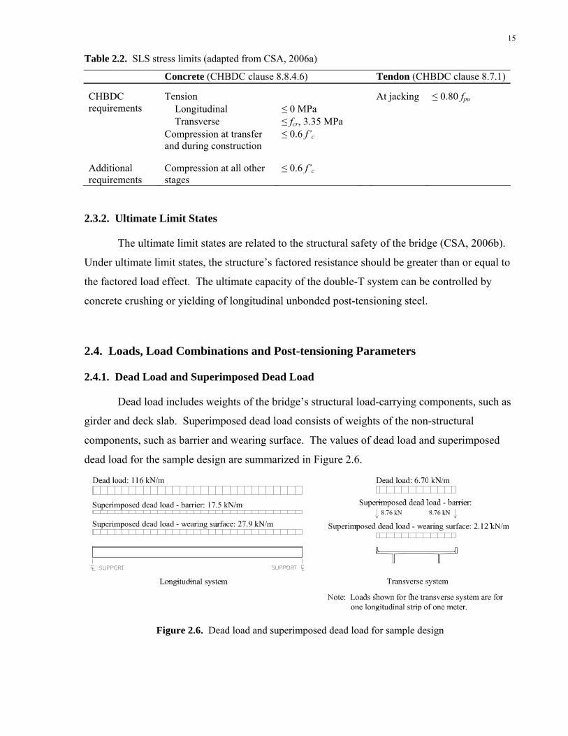
2.4.1. Dead Load and Superimposed Dead Load

Dead load includes weights of the bridge’s structural load-carrying components, such as

girder and deck slab. Superimposed dead load consists of weights of the non-structural

components, such as barrier and wearing surface. The values of dead load and superimposed

dead load for the sample design are summarized in Figure 2.6.

Figure 2.6. Dead load and superimposed dead load for sample design

16

2.4.2 Live Load

CHBDC clause 3.8.3 specifies two live load models – the CL-W Truck and CL-W Lane

Load model, both shown in Figure 2.7. The CL-W Truck consists of 5 axles, spaced at given

distances. The CL-W Lane Load is a combination of 80% of the CL-W Truck Load and a 9

kN/m uniformly distributed load. In the sample design, the CL-625-ONT model is used.

Figure 2.7. CL-W and CL-625-ONT live load models (adapted from CSA, 2006a)

In analysis, the CL-W live load is applied to each design lane of the bridge. Design

lanes are defined by the bridge’s deck width and can be different from the actual travelled lanes

(CSA, 2006b). For the sample design which has a travelled deck width of 13.2 m, there should

be three design lanes according to CHBDC (Figure 2.8). When more than one design lane is

loaded, the total load should be reduced by the multi-lane reduction factor listed in Figure 2.8.

Figure 2.8. Design lane layout

17

The vibration and impact from the travelling vehicles may magnify the live load effect

on the structure. To account for this, CHBDC specifies a dynamic load allowance, which is

expressed as a percentage of the CL-W Truck and added to the static live load (CSA, 2006a). In

an analysis where all axles of the CL-W Truck are considered, the dynamic load allowance is

taken as 0.25, which means that the total live load effect should be increased by 25%. The

dynamic load allowance is only applicable to the CL-W Truck load.

2.4.3. Post-tensioning Parameters

The sample design utilizes two orthogonal systems of prestressing. While the bridge

girder is post-tensioned longitudinally with external unbonded tendons, the deck slab is

transversely post-tensioned with internal bonded tendons. Parameters related to the two systems

of post-tensioning are summarized in Table 2.3. For the transverse tendons, the jacking stress is

assumed to be at the upper limit specified by CHBDC, which is 80% fpu. The loss of prestress is

estimated to be a lump sum of 20% fpu, which is an average along the length of the tendon. Thus

the prestress in transverse post-tensioning after all losses is 60% fpu. The maximum stress in the

transverse post-tensioning tendon is assumed to be 90% fpu. Compared to the transverse system,

the longitudinal post-tensioning system with external unbonded tendons requires a more detailed

evaluation on prestress losses under SLS and the level of stress under ULS. Details on these

two subjects are presented later in Section 2.7.3 and 2.7.4 with other topics related to

longitudinal flexure.

Table 2.3. Post-tensioning parameters

Longitudinal system Transverse System

Tendon type External unbonded Internal bonded

Stress at Jacking 80% fpu 80% fpu

SLS

67% fpu after all losses 74% fpu at 28 days (Section 2.8.2)

60% fpu (with estimated lump-sum losses)

ULS

81% fpu (Section 2.8.4)

90% fpu

The longitudinal post-tensioning of the double-T system involves a two-stage operation

to reduce the overall negative flexural demand on the bridge girder during the stressing of

tendons. During this operation, tendons are separated into two groups and stressed in two

separate stages. Four out of the six tendons are stressed first following the erection of

segments. These tendons are designated as Stage I tendons. Afterwards, prior to the stressing

18

of the remaining two tendons, barriers and wearing surface are placed. This allows both dead

load and super-imposed dead load to be engaged during the second stage of prestressing. As a

result of the increase in gravity load, the net negative flexure in the system is reduced. Finally,

the remaining two tendons are stressed. The basic sequence of construction is summarized in

the following:

1. Erect all girder segments.

2. Stress stage I post-tensioning tendons.

3. Place deck slab wearing surface and barriers.

4. Stress stage II post-tensioning tendons.

The time elapsed between stage I and stage II post-tensioning is assumed to be 28 days.

2.4.4. Load Factors and Load Combinations

CHBDC specifies two SLS and nine ULS load combinations. The ones that are

applicable to the current design are as follows:

SLS Combination 1: 1.00 D + 0.90 L

ULS Combination 1: αD D + 1.70 L

where D represents dead load and superimposed dead load while L represents live load. The

range of αD is summarized in Table 2.4.

Table 2.4. Load factors (CSA, 2006a, clause 3.5.1)

Max. Min.

Dead Load (Precast) 1.10 0.95 Superimposed Dead Load - Barrier (Cast-in-place) 1.20 0.90 Superimposed Dead Load - Wearing Surface 1.50 0.65

For the longitudinal system which involves a staged construction sequence, it is

necessary to expand the load combinations specified by CHBDC to account for loadings during

each stage of the construction as well as the final service stage. The preliminary design for the

double-T system indicates that there are four critical load cases for each of the load

combinations specified by CHBDC. They are schematically illustrated in Table 2.5. The load

factors associated with each load combination are selected to maximize the overall load effect in

each load case.

Table 2.5. Load combinations for the double-T sample design

Load Factor - α Case Combination Schematic DL SDL - B SDL - WS LL P

SLS 1A DL + P1j

1 0 0 0 1

1B DL + SDL + P128 days

1 1 1 0 1

1C DL + SDL + P128days + P2j

1 1 1 0 1

1D DL + SDL + P1∞ + P2∞ + LL

1 1 1 0.9 1

ULS 1A DL + P1j 0.95 0 0 0 1.2* 1B DL + SDL + P1ULS Refer to above 1.1 1.2 1.5 0 1 1C DL + SDL + P128 days + P2j SLS cases 0.95 0.9 0.65 0 1.2*

1D DL + SDL + P1ULS + P2ULS + LL

1.1 1.2 1.5 1.7 1

*The load factor 1.2 is applied to one of tendons only. Notation: DL Dead load P1 Force in stage 1 post-tensioning tendons P2 SDL Super-imposed dead load P1i when tendon stress equals initial jacking stress P2i SDL - B Barrier load P1∞ when tendon stress equals effective prestress after all losses. P2∞ SDL - WS Wearing surface load P1ULS at ULS P2ULS

Force in stage 2 post-tensioning tendons

LL Live load 19

20

Load Combination 1A

This load case takes place immediately following the installation and stressing of stage

one post-tensioning tendons. The stress in the prestressing tendons is taken as the jacking stress.

The post-tensioning force from stage I stressing overcomes the effect of dead load and causes

overall negative moment on the girder.

Load Combination 1B

This load case takes place after the addition of wearing surface and barriers. During

actual construction, false work or erection girder may be left in place or removed at this stage.

This analysis assumes that supporting devices have been removed, thus making the structure

self-supportive. By this time, the stage I tendons have likely lost some of the stresses initially

jacked in. The degree of long-term loss depends on the time elapsed since the stage one

stressing operation, which is assumed to be 28 days in this analysis. This period is estimated

based on the time required to complete work on wearing surface and barriers. This load case is

critical in positive flexure.

Load Combination 1C

This load case occurs immediately after the stressing of stage II post-tensioning tendons.

The stress in the stage II tendons is therefore taken as the jacking stress. The stress in stage I

tendons is again assumed to be the prestress after losses at 28 days. This load case is critical in

negative flexure.

Load Combination 1D

This load case takes place during the structure’s service life, when dead load,

superimposed dead load and live load are all acting on the bridge. For SLS analysis, the tendon

stress is taken as the effective prestress after all losses, while for ULS analysis, the tendon stress

is calculated based on girder’s ULS deformation (see Section 2.7.4).

21

2.5. Transverse System Design

2.5.1. Load Effects

The design process requires an evaluation of the transverse structural response under the

previously discussed loads. Under uniform loads, such as weight of deck slab, barrier and

wearing surface, the deck slab can be treated as a one-way slab with transverse moment constant

along the longitudinal span. The situation under live load is more complicated because the

transverse moment due to concentrated wheel loads varies longitudinally, making it is no longer

appropriate to consider just an arbitrary slice of the girder for the analysis (Gauvreau, 2006).

To evaluate the effect of concentrated live load, elastic influence surfaces are used.

They are diagrams analogous to influence lines, used to calculate load effect at a specific

location on an elastic plate due to applied gravity loads under a given plate geometry and

support condition (Menn, 1990). The design of the double-T girder uses two specific influence

surfaces published by Pucher (1977) – one for the transverse mid-span moment in the deck slab

between the two web supports, the other for the cantilever moment in the deck slab overhang.

2.5.2. Design Approach

For the double-T girder, the transverse span and cantilever of the deck slab are much

longer compared to those of a multi-girder system. As a result, transverse flexure becomes

critical in deck slab design. Web spacing directly affects the transverse flexural demand in the

system. For a box girder, the web-slab junction is often chosen as the quarter points from the

edges of the deck slab so that there is no transverse bending in webs under dead load (Gauvreau,

2006). This is however unnecessary for a double-T girder as the absence of a bottom slab

makes the webs free to rotate. The web spacing instead is chosen to balance the demand and

capacity at the two critical locations – the transverse mid-span of the deck slab and the fixed end

of the deck slab cantilever. A change in web spacing produces opposite effects on the flexural

demands at these two locations. For example, a wider spacing decreases the negative moment at

the end of deck cantilever but increases the positive moment at transverse mid-span. The web

spacing, however, cannot be chosen based solely on the equalization of maximum positive and

negative flexural demand because the positive and negative flexural capacity at the two

locations are different and depends on the transverse post-tensioning design.

22

The deck slab is post-tensioned transversely with flat-duct tendons each containing four

0.6” diameter strands. Recognizing the pattern of the transverse bending moment, the tendon

profile is made parabolic with the highest elevation at the web-slab conjunction and the lowest

elevation at mid-span (Figure 2.9). The sizing of the post-tensioning tendons is based on

flexural demand in the deck slab. For a segmental bridge, another important constraint is that

segments with the same length should have the same number of tendons except for special

segments such as end and deviation segments. For the double-T sample design, a typical

segment is 2.8 m long. Detailed segment layout is shown in Section 2.9.1.

Figure 2.9. Transverse tendon profile

It is recognized from the above discussion that the transverse flexural design of the

double-T system, including the sizing of the post-tensioning tendons and the optimization of

web spacing, is an integrated process. As illustrated in Figure 2.10, while web spacing affects

flexural demand and capacity, it is also determined based on optimization of the ratio between

these two quantities.

Figure 2.10. Integrated process of transverse flexural design As a starting point of the design process, transverse flexural demand from external load

is plotted as a function of web spacing for the two critical locations in Figure 2.11. Web spacing

is chosen to range from 6.5 m to 8.5 m, which is equivalent to 47% to 62% of total deck width.

Demand on the system shifts toward positive flexure as web spacing increases, and vice versa.

Next, moment capacities at the two critical locations are calculated for SLS and ULS

based on the design criteria given in Section 2.2. For SLS, the moment capacity is defined here

23

as a value under which concrete remains uncracked. Concrete stress under SLS can be

calculated as follows:

, or 3.35 MPaQ Pcr

M MP fA S S

σ = − + − ≤ [2-1]

where MQ is moment due to external load and MP is primary moment due to prestress. By

rearranging the above equation, an expression for SLS moment capacity can be obtained:

max,SLS cr PPM f S MA

⎛ ⎞= + × +⎜ ⎟⎝ ⎠

[2-2]

Mmax, SLS is calculated and plotted in Figure 2.11 for cases of having 2, 3 and 4 tendons in each

segment respectively. The moment capacities under ULS are also calculated and shown in

Figure 2.11.

(a) SLS (b) ULS

Figure 2.11. Flexural demand and capacity of transverse system as a function of web spacing

2.5.3. Final Design

Based on the information shown in Figure 2.11, the final transverse design is set to a

web spacing of 7.9 m and a post-tensioning design of 3 tendons (12 strands) per typical segment.

The actual number of strands required for adequate SLS and ULS behaviour is approximately 10.

However, because a whole number of tendons is used, the total number strands per segment is

increased from 10 to 12. The transverse tendon layout in a typical segment is shown in Figure

2.12. To confirm the adequacy of the design, the transverse structural responses under SLS and

-400.0

-300.0

-200.0

-100.0

0.0

100.0

200.0

6 6.5 7 7.5 8 8.5 9

Web spacing [m]

M[k

N-m

/m]

Positive moment at transverse mid-spanNegative moment at fixed end of deck slab cantilever

3

Maximum moment allowableto ensure σbot≤fcr attransverse mid-span

4 tendons per seg

2

2 tendons per seg34

Maximum moment allowableto ensure σtop≤fcr at fixed

end of cantilever-400.0

-300.0

-200.0

-100.0

0.0

100.0

200.0

6 6.5 7 7.5 8 8.5 9

Web spacing [m]

M[k

N-m

/m]

Positive moment at transverse mid-spanNegative moment at fixed end of deck slab cantilever

Positive moment capacityat transverse mid-span

4 tendons per seg32

2 tendons per seg

3

4Negative momentcapacity at fixed endof cantilever

24

ULS are calculated and summarized in Table 2.6. The SLS stresses are within the limit of 0.6f’c

≤ σ ≤ fcr, or -42 MPa ≤ σ ≤ 3.35 MPa. The ULS capacities at the two critical locations are

greater than the respective demands.

Figure 2.12. Transverse tendon layout in a typical segment Table 2.6. Transverse structural response – deck slab

SLS ULS σtop σbot Demand Capacity Demand MPa MPa kN-m/m kN-m/m Capacity

Mid-span between webs -7.702 1.729 119 146 0.81 Cantilever fixed end 1.336 -4.920 -215 -284 0.76

2.6. Torsion and Live Load Distribution

In this section, torsion and live load distribution are evaluated using two approaches.

The first one is an analytical approach based on Menn’s (1990) method of calculating torsion in

a double-T system (Section 2.6.1). This is a simplified method that does not account for the

stiffness of diaphragms in the structure. The second approach is a grillage model analysis

(Section 2.6.2). This method accounts for the presence of diaphragms.

2.6.1. Analytical Approach

2.6.1.1. Torsion

Torsion due to eccentric live load needs to be considered in the design process. An

applied eccentric load can be decomposed into a symmetrical and an antisymmetrical

component as shown in Figure 2.13 (Menn, 1990). The symmetrical component induces

bending and shear in the webs while the antisymmetrical component, which is equivalent to an

externally applied torque, causes torsional moment in the structure (Menn, 1990).

25

Figure 2.13. Decomposition of applied eccentric load (adapted from Menn, 1990)

Torsional moment can be resisted by means of closed shear flow or differential web

bending. The former phenomenon is called St. Venant torsion while the latter is usually referred

to as warping torsion. St. Venant torsion is the dominant action for closed sections such as box

girders, because their cross-section geometry provides an efficient closed shear flow path as

shown in Figure 2.14. Open sections, such as a double-T girder, are not as effective in

facilitating closed shear flows, thus need to resist torsion by a combination of St. Venant and

warping action, with the latter being dominant. This relationship can be expressed as:

( ) ( ) ( )= +SV WT x T x T x [2-3]

where TSV(x) and TW(x) denotes St. Venant torsion and warping torsion respectively.

Figure 2.14. Shear flow paths in closed and open cross-sections

The ratio between St. Venant torsion and warping torsion varies along the span and

depends on the cross-section dimensions and span length. Menn (1990) has proposed a

simplified method to approximate the ratio by assuming that its value is constant along the span,

which is expressed as:

( )( )

SV

W

T x kT x

= [2-4]

where k is the constant ratio between St. Venant and warping torsion. Menn (1990) suggests

that, for a conventional double-T girder, the value of k can be approximated as 1/2 for spans

longer than 50m and 1/3 for spans less than 50m.

26

The method to calculate TSV/TW is based on the understanding that compatibility requires

the twist due to St. Venant and warping torsion to be equal at any given point of the span:

( ) ( )SV Wx xθ θ= [2-5]

The twist angle due to warping can be determined from the following equation:

0

2 ( )( )W vw xxb

θ = [2-6]

where wv is the vertical web deflection due to flexure and b0 is the horizontal distance between

the centrelines of two webs (Figure 2.15). The angle due to St. Venant torsion can be derived

from first principals:

1( ) ( )SV SVx T x dx CGK

θ = +∫ [2-7]

where G is the shear modulus, K is the torsional constant, and C is a constant determined from

boundary conditions. K is a geometric property that depends on the cross-section dimensions.

For a double-T girder,

3 30

1 ( ) 2( )3⎡ ⎤≈ +⎣ ⎦s wK t b b h [2-8]

where ts, b and bw are cross-section dimensions shown in Figure 2.15.

Figure 2.15. Double-T cross-section dimension – notations (adapted from Menn, 1990)

Based on the above method, the TSV/TW ratio for the sample design is calculated to be

0.305, indicating that approximately 77% of total torsion is resisted by warping and only 23% is

by St. Venant action. A sample calculation can be found in Appendix A. The result agrees with

the previous discussion on that warping is the dominant action for resisting torsion in an open

cross-section. However, the actual amount of warping torsion is likely smaller than the value

predicted above since this procedure neglects the presence of concrete diaphragms, which

27

provide rigidity in refraining the differential web bending associated with warping action. This

effect will be investigated in the grillage model analysis in Section 2.6.2.

Warping torsion, as illustrated in Figure 2.16, is the phenomenon of differential bending

between two webs. The applied torque due to warping torsion causes the two webs to deflect in

opposite directions and induces additional longitudinal bending in the webs (Menn, 1990). If

the total factored load results in positive flexural demand on the girder, the warping torsion

shown in Figure 2.16 will cause increased bending in Web1 and reduced bending in Web2.

Therefore, the warping component of torsion can be dealt as additional flexural demand in

design.

Figure 2.16. Differential web bending due to warping torsion (adapted from Menn, 1990)

2.6.1.2. Parametric Study on Torsion

A parametric study is carried out to evaluate the effect of change in span length and web

thickness on the distribution of torsion. It is based on Menn’s method of calculating torsion. In

addition to the cross-section of the sample design, three other cross-sections with varying web

thicknesses are proposed to form the basis of the study. As shown in Table 2.7, their

dimensions are identical to those of the sample design cross-section, except for their web

thicknesses which range from 0.4 m to 0.6 m. Three span lengths are investigated – 30 m, 36.6

m, and 45 m. The proposed variation in span and cross-section produces 12 combinations to be

investigated and compared in the study.

The TW/TTOT and TSV/TTOT ratios for the 12 combinations are evaluated and summarized

graphically in Figure 2.17. It is shown that, as the web thickness increases, the percentage of

total torsion attributed to warping is reduced. For the span of 36.6 m, by increasing the web

thickness from 0.3 m to 0.6 m, the amount of warping torsion can be reduced by 9 percentage

points. Wider webs result in less warping torsion and more St. Venant torsion because they

provide a larger area for closed shear flow. This relationship is also confirmed by equation 2-8,

28

which suggests that the torsional stiffness K of a cross-section is a function of the web thickness

cubed. As a result, as the web thickness increases, the value of K increases, and so does the

amount of torsion attributed to St. Venant action. Another trend observed from Figure 2.17 is

that, as span increases, the amount of warping torsion decreases. For example, for a web

thickness of 0.3 m, the percentage of torsion attributed to warping is reduced from 83% to 68%.

Table 2.7. Variables considered in parametric study for torsion Average web thickness [m] Cross-section Span [m]

0.3025 - cross-section of sample design

30 m, 36.6 m, 45 m

0.4

30 m, 36.6 m, 45 m

0.5

30 m, 36.6 m, 45 m

0.6 30 m, 36.6 m, 45 m

In summary, this study indicates that increase in web thickness and span length

produces less warping torsion. As discussed earlier, warping torsion creates differential web

bending and imposes additional flexural demand on one of the two webs in a double-T girder.

This can be seen as a form of unequal load distribution. Since increase in web thickness and

span reduces warping torsion, it would also result in a more equalized load distribution between

the girder webs given that other factors remain constant.

83% 82% 80% 76% 77% 76% 72% 68% 68% 67% 63% 58%

17% 18% 20% 24% 23% 24% 28% 32% 32% 33% 37% 42%

0%

20%

40%

60%

80%

100%

tw= 0.3

03m

0.4m

0.5m

0.6m

tw= 0.3

03m

0.4m

0.5m

0.6m

tw= 0.3

03m

0.4m

0.5m

0.6m

Tsv/Ttot

Tw/Ttot

Span = 30m Span = 36.6m Span = 45m

Tsv - St. Venant torsionTw - warping torsionTtot - total torsion

Figure 2.17. Torsion distribution with varying web thickness and span length

29

2.6.1.3. Live Load Distribution based on Analytical Approach

In a double-T system, the two webs always collectively carry 100% of all live load

applied to the system. If the load is concentric, for a bridge with a straight and unskewed

alignment, it distributes equally between two webs. However, if the applied load is eccentric,

the load becomes unevenly shared. As described in Section 2.6.1.1, an applied eccentric load

can be decomposed into a symmetrical and an antisymmetrical component. The equivalent load

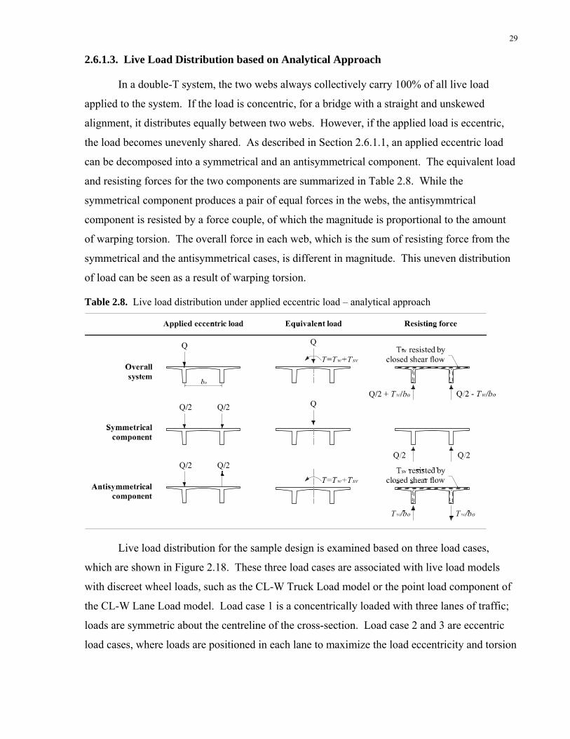
and resisting forces for the two components are summarized in Table 2.8. While the

symmetrical component produces a pair of equal forces in the webs, the antisymmtrical

component is resisted by a force couple, of which the magnitude is proportional to the amount

of warping torsion. The overall force in each web, which is the sum of resisting force from the

symmetrical and the antisymmetrical cases, is different in magnitude. This uneven distribution

of load can be seen as a result of warping torsion.

Table 2.8. Live load distribution under applied eccentric load – analytical approach

Live load distribution for the sample design is examined based on three load cases,

which are shown in Figure 2.18. These three load cases are associated with live load models

with discreet wheel loads, such as the CL-W Truck Load model or the point load component of

the CL-W Lane Load model. Load case 1 is a concentrically loaded with three lanes of traffic;

loads are symmetric about the centreline of the cross-section. Load case 2 and 3 are eccentric

load cases, where loads are positioned in each lane to maximize the load eccentricity and torsion

30

created in the section. Load case 2 bears 2 lanes of traffic whereas Load case 3 bears 3 lanes of

traffic.

Note: W represents CL-W truck axle load.

Figure 2.18. Load cases for evaluating live load distribution

Live load distribution in the sample design is evaluated under the three load cases using

the approach illustrated in Table 2.8, and the results are summarized in Table 2.9. The

calculation procedure (included in Appendix A) assumes that 77% of total torsion is resisted by

warping as calculated in Section 2.6.1.1. Based on this assumption, the concentric load case

Load Case 1 results in an equal sharing of live load, while Load Case 3 results in a 58%-42%

distribution. Among the three cases, Load Case 2 produces the most uneven distribution of live

load, with 80% of total live load being taken by the web on the severe loading side. In addition

to the relative percentage distribution of live load, it is also important to note the absolute

amount of live load carried per web. As shown in Table 2.9, the highest moment per web at

mid-span is 7520 kN-m produced by Load Case 2.

Table 2.9. Live load distribution – analytical approach

Live load distribution: moment at mid-span

Percentage distribution of total live load

Web 1 Web 2 Web 1 Web 2 [kN-m] [kN-m] Load Case 1 6300 6300 50% 50% Load Case 2 7520 1930 80% 20% Load Case 3 7280 5320 58% 42%

Note: (1) W represents CL-W truck axle load; (2) Calculation already accounts for multi-lane reduction factor and dynamic load allowance where applicable.

As shown in Table 2.8, warping torsion is an important quantity that affects the result of

live load distribution. Figure 2.19, which is generated based on the analytical method described

above, illustrates the relationship between the maximum moment per web and the amount of

warping torsion. In general, larger warping torsion produces a higher maximum moment per

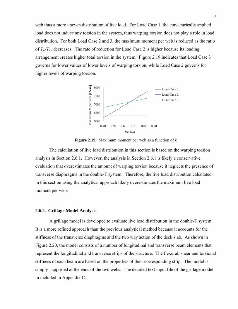
31

web thus a more uneven distribution of live load. For Load Case 1, the concentrically applied

load does not induce any torsion in the system, thus warping torsion does not play a role in load

distribution. For both Load Case 2 and 3, the maximum moment per web is reduced as the ratio

of Tw/Ttot decreases. The rate of reduction for Load Case 2 is higher because its loading

arrangement creates higher total torsion in the system. Figure 2.19 indicates that Load Case 3

governs for lower values of lower levels of warping torsion, while Load Case 2 governs for

higher levels of warping torsion.

6000

6500

7000

7500

8000

0.40 0.50 0.60 0.70 0.80 0.90

Tw/Ttot

Max

imum

M p

er w

eb [k

N-m

] Load Case 1Load Case 2Load Case 3

Figure 2.19. Maximum moment per web as a function of k

The calculation of live load distribution in this section is based on the warping torsion

analysis in Section 2.6.1. However, the analysis in Section 2.6.1 is likely a conservative

evaluation that overestimates the amount of warping torsion because it neglects the presence of

transverse diaphragms in the double-T system. Therefore, the live load distribution calculated

in this section using the analytical approach likely overestimates the maximum live load

moment per web.

2.6.2. Grillage Model Analysis

A grillage model is developed to evaluate live load distribution in the double-T system.

It is a more refined approach than the previous analytical method because it accounts for the

stiffness of the transverse diaphragms and the two way action of the deck slab. As shown in

Figure 2.20, the model consists of a number of longitudinal and transverse beam elements that

represent the longitudinal and transverse strips of the structure. The flexural, shear and torsional

stiffness of each beam are based on the properties of their corresponding strip. The model is

simply-supported at the ends of the two webs. The detailed text input file of the grillage model

in included in Appendix C.

32

Figure 2.20. Grillage model of double-T system

The two eccentric load cases from the previous section (Load Case 2 and Load Case 3)

are considered in the grillage model analysis. Transversely, the CL-W trucks are placed to

maximize the load eccentricity; longitudinally, the loads are positioned to produce the maximum

bending moment at mid-span. The footprints of the truck wheel loads on the bridge deck slab

are illustrated in Figure 2.21. As shown in Figure 2.22, the wheel loads are applied as an

equivalent pair of gravity load and torsional moment on the centroid of the longitudinal strip

they act on.

Load Case 2 Load Case 3

Figure 2.21. Position of truck wheel load for Load Cases 2 and 3

Figure 2.22. Example of equivalent load used in applying wheel load

Figure 2.23 summarizes the results from the grillage model analysis. Member forces

including moment and torsion in webs and transverse diaphragms are plotted in the diagram. A

comparison of the results from the analytical approach and the grillage model is shown in Table

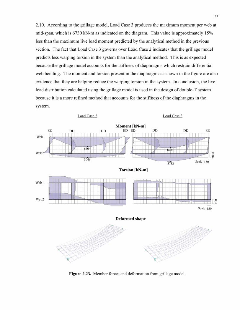
33

2.10. According to the grillage model, Load Case 3 produces the maximum moment per web at

mid-span, which is 6730 kN-m as indicated on the diagram. This value is approximately 15%

less than the maximum live load moment predicted by the analytical method in the previous

section. The fact that Load Case 3 governs over Load Case 2 indicates that the grillage model

predicts less warping torsion in the system than the analytical method. This is as expected

because the grillage model accounts for the stiffness of diaphragms which restrain differential

web bending. The moment and torsion present in the diaphragms as shown in the figure are also

evidence that they are helping reduce the warping torsion in the system. In conclusion, the live

load distribution calculated using the grillage model is used in the design of double-T system

because it is a more refined method that accounts for the stiffness of the diaphragms in the

system.

Load Case 2 Load Case 3

Moment [kN-m]

3046

6404

Web1

ED ED ED EDDD DD DD DD

Web26733

5733 150Scale

2800

Torsion [kN-m]

Scale 150

100

Web1

Web2

Deformed shape

Figure 2.23. Member forces and deformation from grillage model

34

Table 2.10. Comparison of analytical approach and grillage model results [Unit: kN-m]

Analytical approach Grillage model Web 1 Web 2 Web 1 Web 2

Load Case 1 6300 6300 - - Load Case 2 7520 1930 6400 3050 Load Case 3 7280 5320 6730 5730

2.7. Longitudinal Flexure

2.7.1. Unbonded Tendons

Unbonded tendons are commonly used today in bridge and building construction. One

type of application for unbonded tendons is external post-tensioning, where tendons are placed

outside of concrete and enclosed in plastic ducts injected with grout. The underlying principle

of unbonded tendons has a fundamental difference with internal bonded tendons (Menn, 1990).

For bonded tendons, the change in strain in prestressing steel due to deformation (Δεp) equals

the concrete strain at tendon level (εcp) for any given plane section (Figure 2.24). This

compatibility relationship however cannot be applied to unbonded tendons. Due to the lack of

bonding, the tendon strain is not directly related to concrete strain at any one plane. Instead, the

strain depends on the global deformation of the girder and can be determined by integrating the

concrete strain at the level of tendon over the span of the structure (Menn, 1990). The

prestressing steel strain for unbonded tendons can be assumed constant along the span.

Figure 2.24. Compatibility relationship for bonded and unbonded tendons under ultimate limit states Under SLS, as concrete remains uncracked, the girder deformation and the change of

strain in prestressing steel is negligible (Menn, 1990). Thus, the stress in the unbonded tendons

can be taken as the effective prestress (Menn, 1990), which is the tendon stress after all losses.

35

The stress in unbonded tendons under ULS can also be conservatively estimated as the

effective prestress (Menn, 1990). Although this approximation can be sufficient for some of the

preliminary design calculations, it is desirable to determine the actual tendon stress under ULS,

so that better material economy can be achieved. A procedure to calculate unbonded tendon

stress under ULS is described in Section 2.7.4.

For both the SLS and ULS analysis, a reliable value of the effective prestress after all

losses is needed. A procedure for calculating this for girders with unbonded tendons is given in

Section 2.7.2.

2.7.2. Prestress Losses

The effective prestress in tendons under service load is always less than the jacking force

due to prestress losses (Menn, 1990). The prestress losses considered for the sample design

include: (a) friction loss, (b) anchor set loss, (c) loss due to concrete creep and shrinkage, and (d)

relaxation of prestressing steel after transfer. While (a) and (b) are losses at transfer, (c) and (d)

are time-dependent losses taking place over long-term. The losses for the sample design are

calculated with the following procedures and the results are summarized graphically in Figure

2.26.

(a) Friction Loss

Friction loss is due to the friction force between tendon and duct incurred during

stressing of tendons. It is related to the change of tendon alignment in both the vertical and

horizontal plane. The friction loss FR at a distance x away from the jacking end can be

calculated using the following formula (Menn, 1990): ( )(1 )x

oFR f e μα−= − [2-9]

where fo is the jacking stress, α(x) is the angle change between the jacking end and location x,

and μ is the friction coefficient, which varies for different types of post-tensioning systems. For

external unbonded tendons, AASHTO (1998) suggests that μ can be taken as 0.25. Unlike

internal bonded tendons with continuous angle change in their alignment, external unbonded

tendons only incur angle changes at a couple of discreet locations along the span. As a result,

friction loss in external unbonded tendons tends to be lower in comparison with internal bonded

tendons. For the sample design, the total friction loss is calculated to be 14 MPa based on a

value of 0.25 for μ.

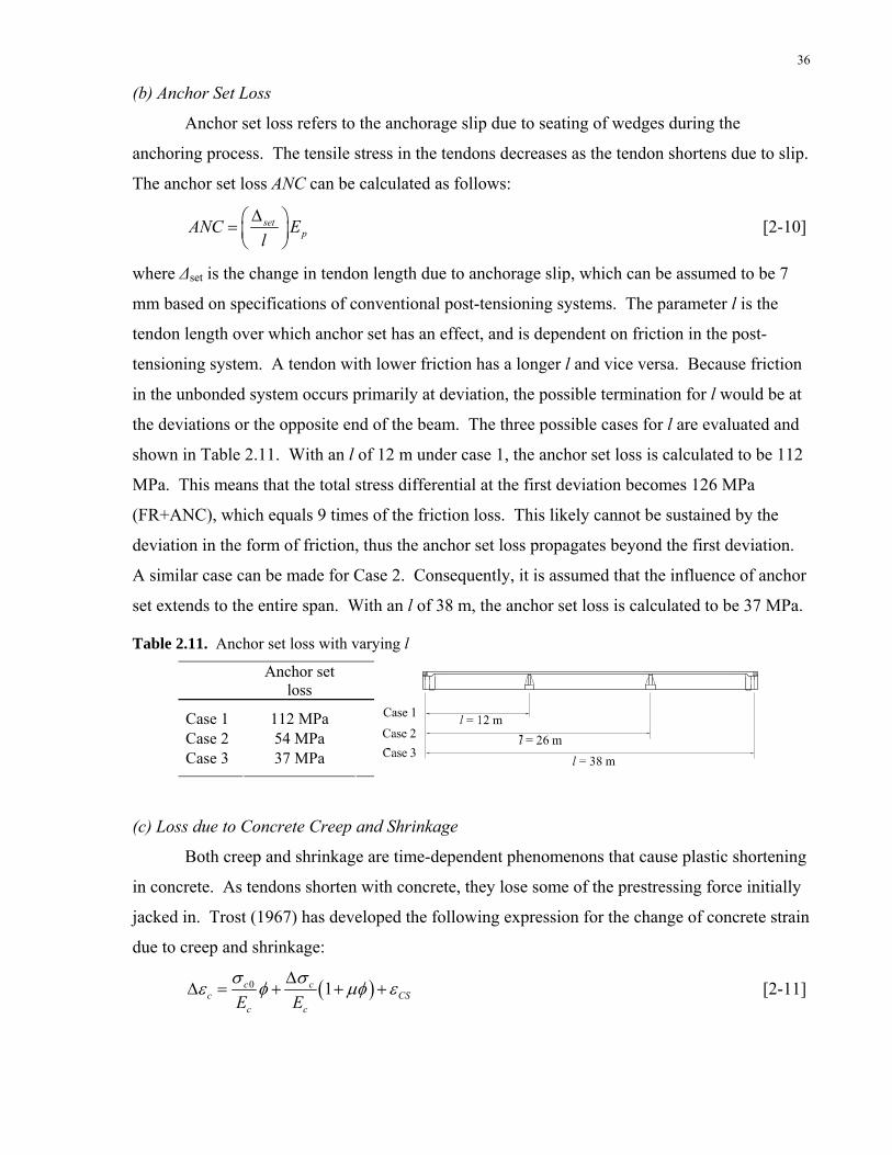
36

(b) Anchor Set Loss

Anchor set loss refers to the anchorage slip due to seating of wedges during the

anchoring process. The tensile stress in the tendons decreases as the tendon shortens due to slip.

The anchor set loss ANC can be calculated as follows:

setpANC E

lΔ⎛ ⎞= ⎜ ⎟

⎝ ⎠ [2-10]

where Δset is the change in tendon length due to anchorage slip, which can be assumed to be 7

mm based on specifications of conventional post-tensioning systems. The parameter l is the

tendon length over which anchor set has an effect, and is dependent on friction in the post-

tensioning system. A tendon with lower friction has a longer l and vice versa. Because friction

in the unbonded system occurs primarily at deviation, the possible termination for l would be at

the deviations or the opposite end of the beam. The three possible cases for l are evaluated and

shown in Table 2.11. With an l of 12 m under case 1, the anchor set loss is calculated to be 112

MPa. This means that the total stress differential at the first deviation becomes 126 MPa

(FR+ANC), which equals 9 times of the friction loss. This likely cannot be sustained by the

deviation in the form of friction, thus the anchor set loss propagates beyond the first deviation.

A similar case can be made for Case 2. Consequently, it is assumed that the influence of anchor

set extends to the entire span. With an l of 38 m, the anchor set loss is calculated to be 37 MPa.

Table 2.11. Anchor set loss with varying l

Anchor set loss

Case 1 112 MPa Case 2 54 MPa Case 3 37 MPa

(c) Loss due to Concrete Creep and Shrinkage

Both creep and shrinkage are time-dependent phenomenons that cause plastic shortening

in concrete. As tendons shorten with concrete, they lose some of the prestressing force initially

jacked in. Trost (1967) has developed the following expression for the change of concrete strain

due to creep and shrinkage:

( )0 1c cc CS

c cE Eσ σε φ μφ εΔ

Δ = + + + [2-11]

37

where σc0 is the initial concrete stress at the level of prestressing steel due to dead load and

prestressing force; φ and μ are the creep coefficient and the aging coefficient respectively; and

εcs(t) is the concrete shrinkage strain. Based on the compatibility relationship of Δεp = εcp

(Figure 2.21), Menn (1990) has derived from equation 2-11 the following formula to calculate

the loss of prestress due to creep and shrinkage for bonded tendons:

( ) [ ]( )

0

1 1c c cs c cn A E A

P tn

ρ σ φ ερ μφ

+Δ =

+ + [2-12]

where n = Ep / Ec and ρ = Ap / Ac. This formula, however, cannot be applied to unbonded

tendons, because the derivation assumes that Δεp = εcp, which does not hold true for unbonded

tendons.

From the same expression by Trost [2-11], Gauvreau (1993) has derived a formula to

calculate creep and shrinkage loss based on the compatibility relationship for unbonded tendons,

which requires that the total change in length in prestressing steel equals the total concrete

deformation at the level of unbonded tendons. This relationship, which assumes that the strain in

prestressing steel is constant along the length of tendon, can be expressed as follows:

( )1p cp

p

x dxl

ε εΔ = ∫ [2-13]

where Δεp is the change in strain in prestressing steel; εcp is the concrete strain at elevation of

tendon; and lp is tendon length. The integration of εcp is over the projected length of tendon.

The formula for creep and shrinkage loss developed by Gauvreau (1993) for unbonded tendons

is as follows:

( )

[ ] ( )

0

2

1

1 1 1

c c cs c cp

c

p c

n A x dx E Al

PAn e x dx

l I

ρ φ σ ε

ρ μφ

⎡ ⎤+⎢ ⎥

⎢ ⎥⎣ ⎦Δ =⎡ ⎤

+ + +⎢ ⎥⎢ ⎥⎣ ⎦

∫

∫ [2-14]

where e(x) is the distance from centroid of the gross uncracked concrete section to the centroid

of unbonded prestressing steel.

38

(a) (b) (c) (a) Nominal creep coefficient versus relative humidity for water-to-cement ratio (W/C) of 0.4 and 0.5 (b) Correction factor k versus time of loading (days / years after casting) (c) Time-varying function f(t-τ) versus time (days / years after casting) for two typical values of hef, where hef = 2Ac/U. Ac is the cross-sectional area and U denotes the exposed perimeter.

Figure 2.25. Parameters in determining creep coefficient φ (Menn, 1990)

The value of μ in equation 2-14 can normally be taken as 0.8 (Menn, 1990). Both the

shrinkage strain and the creep coefficient are time-dependent variables. While εcs can be

determined from charts in Menn (1990), creep coefficient φ can be calculated using the

following equation (Menn, 1990):

( ) ( )( , ) nt k f tφ τ φ τ τ= − [2-15]

where φn is the nominal creep coefficient; k(τ) is a correction factor for the age of concrete at

time of loading; and f(t-τ) is the function accounting for the time-varying property of creep. All

three parameters can be determined graphically from diagrams in Figure 2.25.

Based on the above information, long-term prestress loss due to creep and shrinkage for

the sample design is evaluated for a projected service life of 50 years. Also included in the

calculation is the loss in stage 1 tendons at the time of stage 2 post-tensioning, which was

assumed to be 28 days after the stage 1 operation. The creep and shrinkage losses calculated are

summarized in Table 2.12.

Table 2.12. Loss due to creep and shrinkage and related parameters

Time Shrinkage strain, εcs (Menn, 1990)

Creep coefficient, φ (Menn, 1990)

Loss due to creep and shrinkage

All tendons 50 years -0.298 mm/m 2.00 136 MPa

Stage 1 tendons 28 days -0.105 mm/m 0.50 25 MPa

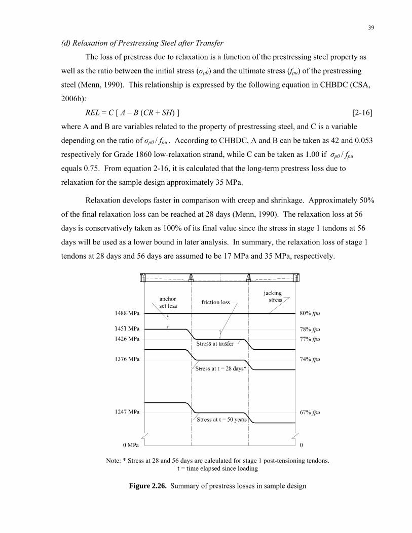
39

(d) Relaxation of Prestressing Steel after Transfer

The loss of prestress due to relaxation is a function of the prestressing steel property as

well as the ratio between the initial stress (σp0) and the ultimate stress (fpu) of the prestressing

steel (Menn, 1990). This relationship is expressed by the following equation in CHBDC (CSA,

2006b):

REL = C [ A – B (CR + SH) ] [2-16]

where A and B are variables related to the property of prestressing steel, and C is a variable

depending on the ratio of σp0 / fpu . According to CHBDC, A and B can be taken as 42 and 0.053

respectively for Grade 1860 low-relaxation strand, while C can be taken as 1.00 if σp0 / fpu

equals 0.75. From equation 2-16, it is calculated that the long-term prestress loss due to

relaxation for the sample design approximately 35 MPa.

Relaxation develops faster in comparison with creep and shrinkage. Approximately 50%

of the final relaxation loss can be reached at 28 days (Menn, 1990). The relaxation loss at 56

days is conservatively taken as 100% of its final value since the stress in stage 1 tendons at 56

days will be used as a lower bound in later analysis. In summary, the relaxation loss of stage 1

tendons at 28 days and 56 days are assumed to be 17 MPa and 35 MPa, respectively.

Note: * Stress at 28 and 56 days are calculated for stage 1 post-tensioning tendons. t = time elapsed since loading

Figure 2.26. Summary of prestress losses in sample design

40

2.7.3. Flexural Response under SLS

The structural response under SLS needs to be evaluated for the load combinations

presented in Section 2.4.4. The magnitude and load factors for dead, superimposed dead and

live load were given in Section 2.4.1 and 2.4.2. The prestressing force used in each load

combination is based on the loss calculation from section 2.7.2. As shown in Figure 2.26,

prestress losses vary along the span. This variation, however, only changes the total

prestressing force in each case by approximately 1%. Due to the relatively small effect of the

variations, the stress in the prestressing steel is assumed to be constant along the span for the

SLS analysis. The prestress values used in the SLS calculation are summarized in Table 2.13.

For load case 1A which represents the loading condition during stage I post-tensioning, the

stress in stage I tendons (fP1) is assumed to be the jacking stress, 0.80 fpu. For load case 2, which

describes the loading just prior to stage II post-tensioning, fP1 is taken as the prestress after 28

days, which is 0.74 fpu, because stage II post-tensioning is assumed to commence 28 days after

stage I. Load case 1C takes place shortly after load case 1B during stage II post-tensioning

operation. Under this load case, fP1 is assumed to still be at 0.74 fpu, while fP2 is taken as the

jacking stress, 0.80 fpu. Finally, load case 1D accounts for the load combination during the

bridge’s service life. fP1 and fP2 are taken as the prestress after all losses for a period of 50 years.

Table 2.13. Stress in post-tensioning steel under SLS

Case Combination fP1 fP2 SLS 1A DL + P1 80% fpu 0 1B DL + SDL + P1 74% fpu 0 1C DL + SDL + P1 + P2 74% fpu 80% fpu 1D DL + SDL + P1 + P2 + LL 67% fpu 67% fpu

The concrete stresses at the girder’s top and bottom fibre are calculated for the four load

combinations and shown in Figure 2.27. Stresses are not shown for girder ends, because it is not

appropriate to use methods based on the principle of plane sections to evaluate these disturbed

regions with not only changing geometry but also large concentrated forces from the post-

tensioning anchorages. Based on St. Venant principle, the length of the disturbed region is

approximated as the depth of the girder, which is 2 m (Schlaich, 1987). The end region will be

analyzed explicitly with strut-and-tie models in Section 2.8.

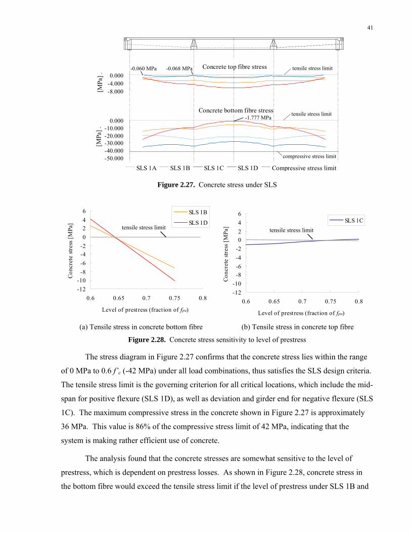
41

Concrete top fibre stress

-8.000-4.0000.000

[MPa

].Concrete bottom fibre stress

-50.000-40.000-30.000-20.000-10.000

0.000

[MPa

].

SLS 1A SLS 1B SLS 1C SLS 1D Compressive stress limit

-0.060 MPa

-1.777 MPa

-0.068 MPa tensile stress limit

tensile stress limit

compressive stress limit

Figure 2.27. Concrete stress under SLS

-12-10

-8-6-4-20246

0.6 0.65 0.7 0.75 0.8

Level of prestress (fraction of fpu)

Conc

rete

stres

s[M

Pa]

SLS 1B

SLS 1D

-12-10

-8-6-4-20246

0.6 0.65 0.7 0.75 0.8

Level of prestress (fraction of fpu)

Conc

rete

stres

s[M

Pa]

SLS 1Ctensile stress limittensile stress limit

(a) Tensile stress in concrete bottom fibre (b) Tensile stress in concrete top fibre

Figure 2.28. Concrete stress sensitivity to level of prestress

The stress diagram in Figure 2.27 confirms that the concrete stress lies within the range

of 0 MPa to 0.6 f’c (-42 MPa) under all load combinations, thus satisfies the SLS design criteria.

The tensile stress limit is the governing criterion for all critical locations, which include the mid-

span for positive flexure (SLS 1D), as well as deviation and girder end for negative flexure (SLS

1C). The maximum compressive stress in the concrete shown in Figure 2.27 is approximately

36 MPa. This value is 86% of the compressive stress limit of 42 MPa, indicating that the

system is making rather efficient use of concrete.

The analysis found that the concrete stresses are somewhat sensitive to the level of

prestress, which is dependent on prestress losses. As shown in Figure 2.28, concrete stress in

the bottom fibre would exceed the tensile stress limit if the level of prestress under SLS 1B and

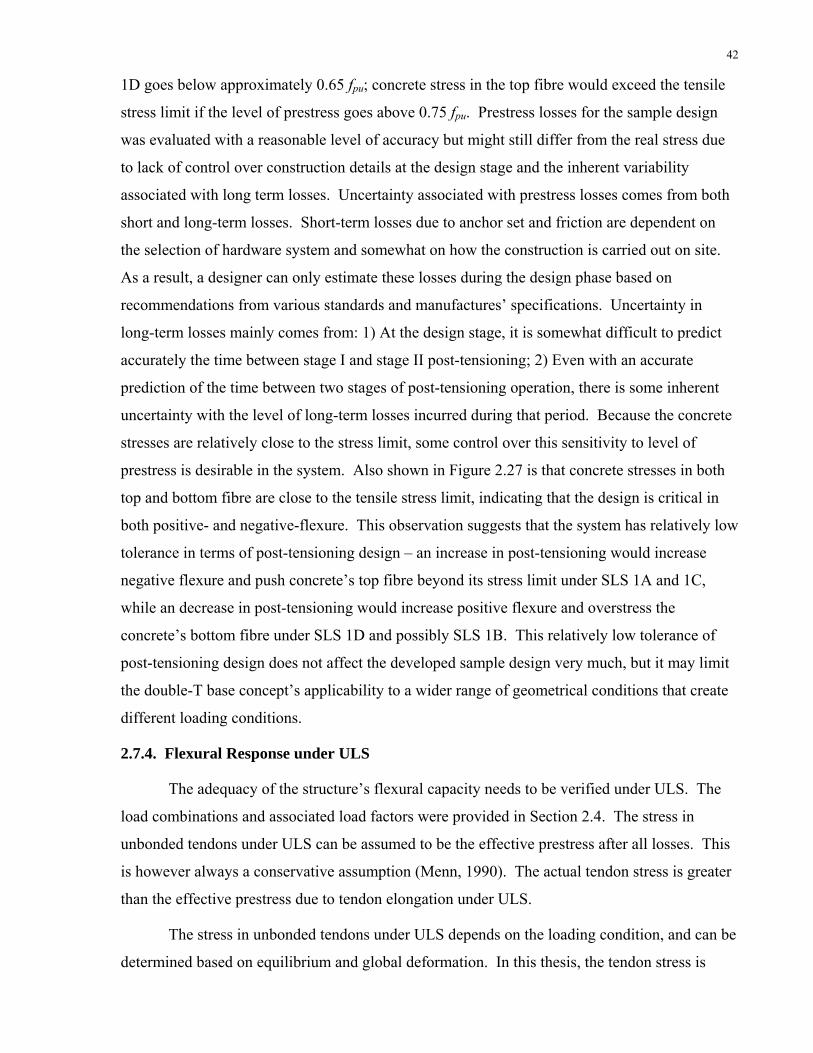
42

1D goes below approximately 0.65 fpu; concrete stress in the top fibre would exceed the tensile

stress limit if the level of prestress goes above 0.75 fpu. Prestress losses for the sample design

was evaluated with a reasonable level of accuracy but might still differ from the real stress due

to lack of control over construction details at the design stage and the inherent variability

associated with long term losses. Uncertainty associated with prestress losses comes from both

short and long-term losses. Short-term losses due to anchor set and friction are dependent on

the selection of hardware system and somewhat on how the construction is carried out on site.

As a result, a designer can only estimate these losses during the design phase based on

recommendations from various standards and manufactures’ specifications. Uncertainty in

long-term losses mainly comes from: 1) At the design stage, it is somewhat difficult to predict

accurately the time between stage I and stage II post-tensioning; 2) Even with an accurate

prediction of the time between two stages of post-tensioning operation, there is some inherent

uncertainty with the level of long-term losses incurred during that period. Because the concrete

stresses are relatively close to the stress limit, some control over this sensitivity to level of

prestress is desirable in the system. Also shown in Figure 2.27 is that concrete stresses in both

top and bottom fibre are close to the tensile stress limit, indicating that the design is critical in

both positive- and negative-flexure. This observation suggests that the system has relatively low

tolerance in terms of post-tensioning design – an increase in post-tensioning would increase

negative flexure and push concrete’s top fibre beyond its stress limit under SLS 1A and 1C,

while an decrease in post-tensioning would increase positive flexure and overstress the

concrete’s bottom fibre under SLS 1D and possibly SLS 1B. This relatively low tolerance of

post-tensioning design does not affect the developed sample design very much, but it may limit

the double-T base concept’s applicability to a wider range of geometrical conditions that create

different loading conditions.

2.7.4. Flexural Response under ULS

The adequacy of the structure’s flexural capacity needs to be verified under ULS. The

load combinations and associated load factors were provided in Section 2.4. The stress in

unbonded tendons under ULS can be assumed to be the effective prestress after all losses. This

is however always a conservative assumption (Menn, 1990). The actual tendon stress is greater

than the effective prestress due to tendon elongation under ULS.

The stress in unbonded tendons under ULS depends on the loading condition, and can be

determined based on equilibrium and global deformation. In this thesis, the tendon stress is

43

evaluated by a method that equilibrates tendon elongation due to tendon force (ΔlPF) with

tendon elongation due to deformation (ΔlPD). For an assumed tendon force Pi, ΔlPF can be

calculated from the following equation:

( )0

iPF P

P P

P Pl l

A E∞−

Δ = [2-17]

where P∞ is the effective prestress after all losses and lp0 is the tendon length when the force in

tendon is P∞. For a structural member with external load Qf and tendon force Pi, ΔlPF can be

calculated as follows:

( )PD cPl x dxεΔ = ∫ [2-18]

where εcp is the concrete strain at level of prestressing tendon due to Qf and Pi. The calculation

procedure is an iterative process in which the value of Pi is assumed and adjusted until the

tendon elongation calculated from equation 2-17 and 2-18 are equal. The final solution from the

iteration is a tendon force that is compatible with the member deformation under external load

Qf. It is also useful to determine the minimum prestressing force Pmin required for equilibrating

external loads. The value of Pmin and the tendon yield force Py serve as the lower and upper

bound of the actual tendon force. The iterative procedure is schematically illustrated in Figure

2.29.

Figure 2.29. Iterative procedure for calculating post-tensioning force in unbonded tendons under ULS

Preliminary calculations indicate that concrete remains within the uncracked and linear

elastic range under load combination ULS 1A and 1B (Figure 2.30). Thus it is clear that

structural capacity is greater than demand under these two load cases. The remaining load cases

to be checked are ULS 1C and 1D.

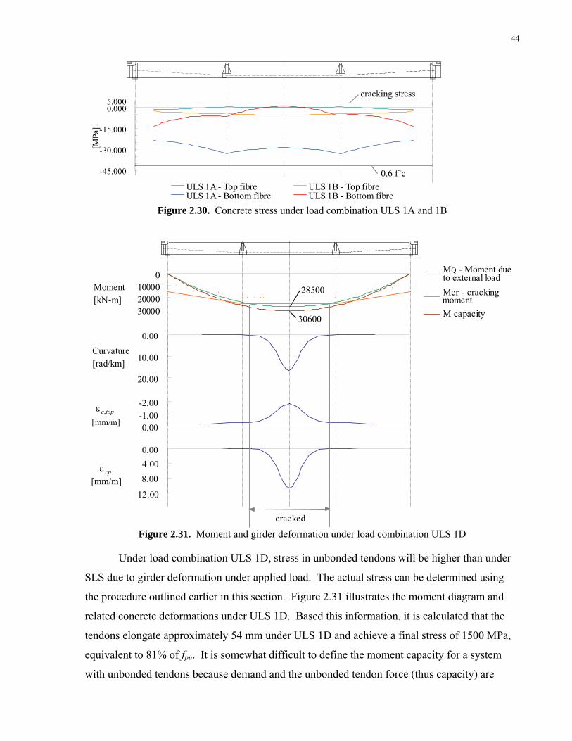
44

-45.000

-30.000

-15.000

0.0005.000

[MPa

] .

ULS 1A - Top fibre ULS 1B - Top fibreULS 1A - Bottom fibre ULS 1B - Bottom fibre

cracking stress

0.6 f’c

Figure 2.30. Concrete stress under load combination ULS 1A and 1B

0100002000030000

Moment[kN-m]

MQ - Moment dueto external loadMcr - crackingmomentM capacity

-2.00-1.000.00[mm/m]

0.00

10.00

20.00

Curvature[rad/km]

0.004.008.00

12.00[mm/m]

,c topε

cpε

28500

30600

cracked Figure 2.31. Moment and girder deformation under load combination ULS 1D

Under load combination ULS 1D, stress in unbonded tendons will be higher than under

SLS due to girder deformation under applied load. The actual stress can be determined using

the procedure outlined earlier in this section. Figure 2.31 illustrates the moment diagram and

related concrete deformations under ULS 1D. Based this information, it is calculated that the

tendons elongate approximately 54 mm under ULS 1D and achieve a final stress of 1500 MPa,

equivalent to 81% of fpu. It is somewhat difficult to define the moment capacity for a system

with unbonded tendons because demand and the unbonded tendon force (thus capacity) are

45

interrelated. The moment capacity diagram shown in Figure 2.31 is calculated by magnifying

the total load on the girder until the unbonded tendon stress reaches the yield stress. Thus the

curve can be interpreted approximately as the upper limit for demand. It is shown in Figure

2.31 that the upper limit is approximately 7% higher than the actual demand on the girder.

Load combination ULS 1C accounts for the loading condition during stage II post-

tensioning. As shown in Figure 2.32, the negative moment due to prestressing force under this

load case is larger than the positive moment from to external load, resulting in overall negative

bending in the girder. Thus, unlike ULS 1D where tendons need to gain additional stress to

maintain equilibrium with external applied load, the tendon stress under ULS 1C remains

unchanged at 0.74 fpu for stage I tendons and 0.80 fpu for stage II tendons. An estimation of

concrete stress under ULS 1C using elastic method indicates that the maximum tensile stress

and compressive stress in the concrete are 1.5 MPa and -48 MPa, respectively. This suggests

that concrete remains uncracked but goes slightly beyond the linear elastic range under ULS 1C.

The negative flexural capacity of the girder is thus checked for this load combination. With the

known prestressing force P, the negative flexural capacity of the girder is calculated with P

treated as external load. The capacity of -17350 kN-m, as shown in Figure 2.33, is greater than

the total demand from MQ and MP (-11460 kN-m) shown in Figure 2.32.

-20000

0

20000

40000

Moment[kN-m]

MQ - Moment dueto external loadMQ + MP

M capacity (P asload)

-11460

-17220

Figure 2.32. Moment diagram under load combination ULS 1C

Note: Prestressing force is treated as load instead of internal resistance.

Figure 2.33. Negative flexural capacity of girder under load combination ULS 1C

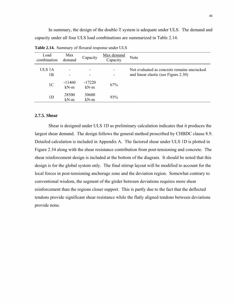
46

In summary, the design of the double-T system is adequate under ULS. The demand and

capacity under all four ULS load combinations are summarized in Table 2.14.

Table 2.14. Summary of flexural response under ULS

Load combination

Max demand Capacity Max demand

Capacity Note

ULS 1A - - - 1B - - -

Not evaluated as concrete remains uncracked and linear elastic (see Figure 2.30)

1C -11460 kN-m

-17220 kN-m 67%

1D 28500 kN-m

30600 kN-m 93%

2.7.5. Shear

Shear is designed under ULS 1D as preliminary calculation indicates that it produces the

largest shear demand. The design follows the general method proscribed by CHBDC clause 8.9.

Detailed calculation is included in Appendix A. The factored shear under ULS 1D is plotted in

Figure 2.34 along with the shear resistance contribution from post-tensioning and concrete. The

shear reinforcement design is included at the bottom of the diagram. It should be noted that this

design is for the global system only. The final stirrup layout will be modified to account for the

local forces in post-tensioning anchorage zone and the deviation region. Somewhat contrary to

conventional wisdom, the segment of the girder between deviations requires more shear

reinforcement than the regions closer support. This is partly due to the fact that the deflected

tendons provide significant shear resistance while the flatly aligned tendons between deviations

provide none.

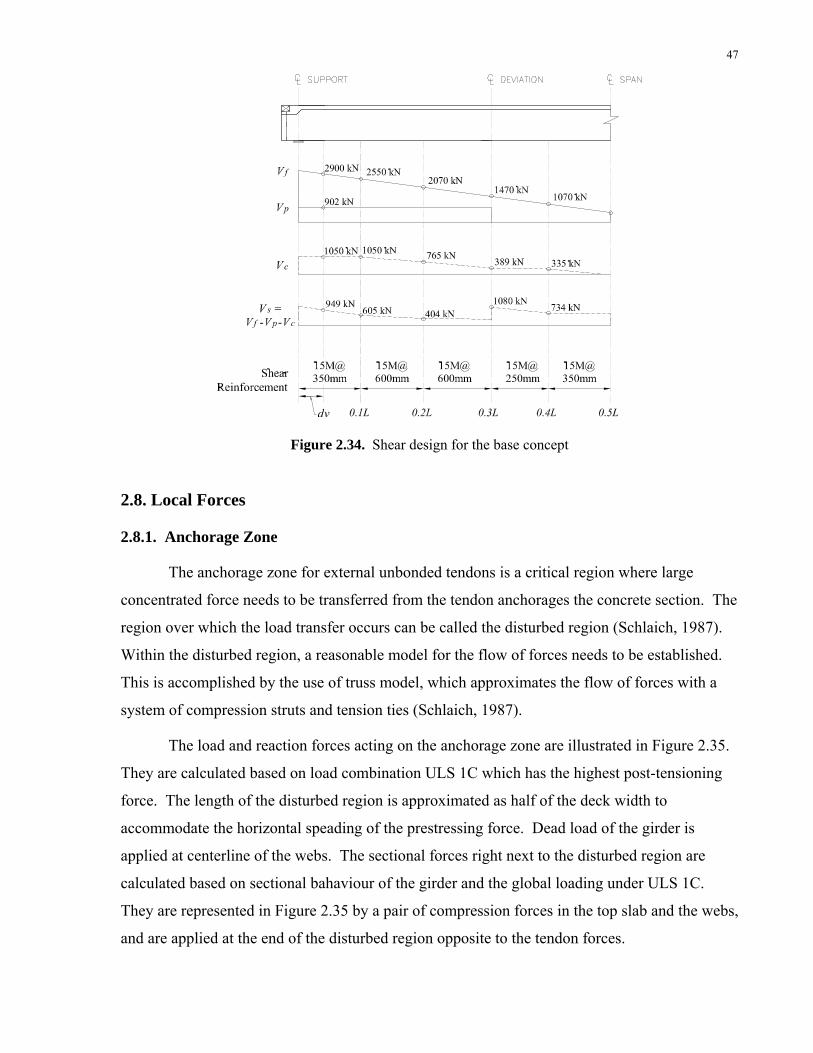
47

Figure 2.34. Shear design for the base concept 2.8. Local Forces

2.8.1. Anchorage Zone

The anchorage zone for external unbonded tendons is a critical region where large

concentrated force needs to be transferred from the tendon anchorages the concrete section. The

region over which the load transfer occurs can be called the disturbed region (Schlaich, 1987).

Within the disturbed region, a reasonable model for the flow of forces needs to be established.

This is accomplished by the use of truss model, which approximates the flow of forces with a

system of compression struts and tension ties (Schlaich, 1987).

The load and reaction forces acting on the anchorage zone are illustrated in Figure 2.35.

They are calculated based on load combination ULS 1C which has the highest post-tensioning

force. The length of the disturbed region is approximated as half of the deck width to

accommodate the horizontal speading of the prestressing force. Dead load of the girder is

applied at centerline of the webs. The sectional forces right next to the disturbed region are

calculated based on sectional bahaviour of the girder and the global loading under ULS 1C.

They are represented in Figure 2.35 by a pair of compression forces in the top slab and the webs,

and are applied at the end of the disturbed region opposite to the tendon forces.

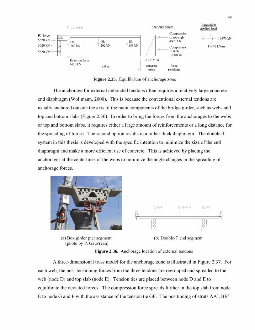
48

Figure 2.35. Equilibrium of anchorage zone

The anchorage for external unbonded tendons often requires a relatively large concrete

end diaphragm (Wollmann, 2000). This is because the conventional external tendons are

usually anchored outside the axis of the main components of the bridge girder, such as webs and

top and bottom slabs (Figure 2.36). In order to bring the forces from the anchorages to the webs

or top and bottom slabs, it requires either a large amount of reinforcements or a long distance for

the spreading of forces. The second option results in a rather thick diaphragm. The double-T

system in this thesis is developed with the specific intention to minimize the size of the end

diaphragm and make a more efficient use of concrete. This is achieved by placing the

anchorages at the centerlines of the webs to minimize the angle changes in the spreading of

anchorage forces.

(a) Box girder pier segment (b) Double-T end segment (photo by P. Gauvreau)

Figure 2.36. Anchorage location of external tendons

A three-dimensional truss model for the anchorage zone is illustrated in Figure 2.37. For

each web, the post-tensioning forces from the three tendons are regrouped and spreaded to the

web (node D) and top slab (node E). Tension ties are placed between node D and E to

equilibrate the deviated forces. The compression force spreads further in the top slab from node

E to node G and F with the assistance of the tension tie GF. The positioning of struts AA’, BB’

49

and CC’ in one plane allows the use of a relative thin diaphragm. The forces in struts and ties

are calculated from the loads described in Figure 2.35 and are based on equilibrium at each joint.

Concrete stresses in the compression struts are found to be non-critical. The quantity of

reinforcements required in the region, which is based on the forces in the tension ties, is


5001780

1290

12000

3000

50103000

2420

2420

Top view

Side view

Isometric view

Figure 2.37. Anchorage zone truss model [Unit: kN]

Table 2.15. Anchorage zone reinforcing steel

Force Reinforcement

Tie DE 1290 kN 20M@120mm, for a 1.5m wide band centred at tie AB Tie GF 1780 kN Two additional 4-0.6" tendons in the top slab

As shown in the above discussion, by placing the external tendon anchorages at the

centerlines of webs, the amount of forces required for spreading the anchorage forces is reduced

and so is the required dimension of the end diaphragm. One implication of this anchorage

placement is that the angle of which the tendons extrude from the concrete webs is relatively flat

(shown in top view of Figure 2.37). To resolve this issue, the webs are widened for a certain

distance from the end of the girder. More details on the widened webs are shown in Section

2.9.1.

2.8.2. Deviation

Similar as tendon anchorages, deviations also create large concentrated forces in the

structure. The flow of forces is again analyzed by the use of truss model, which is illustrated in

50

Figure 2.38. The forces are calculated under ULS 1C which has the highest post-tensioning

force among all load cases. The reinforcing steel required based on this truss model is


Figure 2.38. Deviation truss model

Table 2.16. Deviation reinforcing steel

Force Reinforcement

Horizontal tie 470 kN 20M@170mm, for a 1.5m band centred at deviation Vertical tie 900 kN One additional 4-0.6" tendon in the top slab at deviation

2.9. Construction

2.9.1. Precast Segment Design

The double-T bridge concept will be constructed using precast segmental method. The

segment layout for the design example is shown in Figure 2.39. For transportation reasons, the

length of every segment is limited under 3 m.

Figure 2.39. Segment layout There are four types of segments in the sample design:

1. Interior segment (IS) (Figure 2.40 a)

These are regular segments with no special modifications.

2. Modified interior segment (MIS) (Figure 2.40 b)

These segments are positioned next to the end segments. Their geometry is the same as

interior segments except that their webs are slightly widened to accommodate post-tensioning

tendons extruding from concrete.

51

3. Deviation segment (DS) (Figure 2.40 c)

The deviation segment requires a full or partial concrete diaphragm to support the tendon

deviators and to accommodate the flow of forces from the tendon deviation. For box-girder

bridges, partial diaphragms with an access opening are usually used to facilitate future bridge

inspection. The double-T girder bridge however does not necessarily require such an opening in

the diaphragm because all its concrete surfaces are readily accessible for inspection from

exterior. The diaphragm dimensions are adapted from ASBI standard drawings (2008).

4. End segment (ES) (Figure 2.40 d)

The relatively complicated geometry of the end segment is to accommodate the

following:

a. Anchors of the longitudinal post-tensioning tendons;

b. Flow of forces from tendon anchorages to concrete sections, as described in Section

2.8.1;

c. Recess for expansion joint;

d. Contact surface for bearing plate.

Detailed segment drawings with complete dimensioning can be found in Appendix A.

The actual dimensions are based on ASBI standard drawings (2008) and the anchorage zone

truss model analysis.

Side view Cross-section view Isometric view

Figure 2.40. Segment geometry

(a) Interior segment (IS)

(b) Modified interior segment (MIS)

(c) Deviation segment (DS)

(d) End segment (ES)

52

2.9.2. Precast Concrete Forming

Segments will be precasted with match-cast technology, which produces perfectly-fitted

joints by casting a new segment against a dry mate segment. Segments produced by such

method can be erected on site speedily without the need of cast-in-place concrete or grout. As

discussed in Chapter 1, segmental construction of box girder bridges usually involves the use of

a core form, of which cost is rather high and can only be justified for long bridges. For the

double-T system, the absence of a bottom slab frees the construction from the need of a core

form and subsequently creates flexibility in the choices of forming method. The double-T

segments can be casted with relative inexpensive plywood formwork as shown in Figure 2.41.

The cost can be further reduced by employing a system of formwork modules, which are created

based on the common geometrical elements shared by each type of segment. These modules

can be used in various combinations to form the different types of segment in the system.

Figure 2.41. Schematic illustration of formwork for an interior segment

2.9.3. Girder Erection

The construction sequence for the superstructure of a single-span double-T bridge is as

follows:

1. Erect precast girders;

2. Stress stage I post-tensioning tendons;

3. Place wearing surface and barriers;

4. Stress stage II post-tensioning tendons.

The girder segments can be erected on either false work or erection girders. The first

option is more economical if access from below the bridge is relatively non-restrictive.

Otherwise, the second method is a more suitable option. Both types of erection systems need to

provide a platform below the girder for personnel to stand on during the grouting of external

post-tensioning tendons. A platform can be added onto false work with relative ease. Erection

girders, on the other hand, needs to be specifically designed to be able to accommodate such a

Wooden form Platform

53

platform. A sample design of an under-slung erection girder with overhanging platform is

shown in Figure 2.42.

Figure 2.42. Erection girder with overhanging platform

2.10. Final Remarks

A double-T system with pure external unbonded post-tensioning is developed in this

chapter. The concrete section with two slender webs not only reduces the overall concrete and

dead load of the structure, but also improves the live load distribution in comparison with

conventional slab-on-girder system with multiple girders. A detailed comparison of the two

types of systems will be presented later in Chapter 6. The double-T system will be constructed

with precast segmental method, which allows the bridge to be built rapidly with relatively low

impact on site. The simplicity of the double-T section allows for easy forming and flexibility in

construction.

The sample design of the double-T base concept is governed by longitudinal flexure

under SLS. It is found in the SLS analysis that the structure is somewhat sensitive to the

assumptions related to loss of prestress and the amount of the post-tensioning in the system.

This finding does not affect the developed sample design very much, but it may limit the

double-T base concept’s applicability to a wider range of geometrical requirements that create

different loading conditions. To resolve this limitation, two alternative double-T concepts with

a blend of prestressed and non-prestressed primary reinforcements will be examined in the

following two chapters. They are modifications of the base concept with reduced amounts of

post-tensioning and supplementary non-prestressed reinforcements.

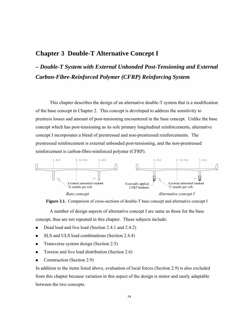
Chapter 3 Double-T Alternative Concept I

– Double-T System with External Unbonded Post-Tensioning and External

Carbon-Fibre-Reinforced Polymer (CFRP) Reinforcing System

This chapter describes the design of an alternative double-T system that is a modification

of the base concept in Chapter 2. This concept is developed to address the sensitivity to

prestress losses and amount of post-tensioning encountered in the base concept. Unlike the base

concept which has post-tensioning as its sole primary longitudinal reinforcements, alternative

concept I incorporates a blend of prestressed and non-prestressed reinforcements. The

prestressed reinforcement is external unbonded post-tensioning, and the non-prestressed

reinforcement is carbon-fibre-reinforced polymer (CFRP).

Base concept Alternative concept I

Figure 3.1. Comparison of cross-sections of double-T base concept and alternative concept I

A number of design aspects of alternative concept I are same as those for the base

concept, thus are not repeated in this chapter. These subjects include:

Dead load and live load (Section 2.4.1 and 2.4.2)

SLS and ULS load combinations (Section 2.4.4)

Transverse system design (Section 2.5)

Torsion and live load distribution (Section 2.6)

Construction (Section 2.9)

In addition to the items listed above, evaluation of local forces (Section 2.9) is also excluded

from this chapter because variation in this aspect of the design is minor and easily adaptable

between the two concepts.

54

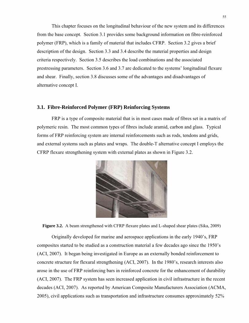
55

This chapter focuses on the longitudinal behaviour of the new system and its differences

from the base concept. Section 3.1 provides some background information on fibre-reinforced

polymer (FRP), which is a family of material that includes CFRP. Section 3.2 gives a brief

description of the design. Section 3.3 and 3.4 describe the material properties and design

criteria respectively. Section 3.5 describes the load combinations and the associated

prestressing parameters. Section 3.6 and 3.7 are dedicated to the systems’ longitudinal flexure

and shear. Finally, section 3.8 discusses some of the advantages and disadvantages of

alternative concept I.

3.1. Fibre-Reinforced Polymer (FRP) Reinforcing Systems

FRP is a type of composite material that is in most cases made of fibres set in a matrix of

polymeric resin. The most common types of fibres include aramid, carbon and glass. Typical

forms of FRP reinforcing system are internal reinforcements such as rods, tendons and grids,

and external systems such as plates and wraps. The double-T alternative concept I employs the

CFRP flexure strengthening system with external plates as shown in Figure 3.2.

Figure 3.2. A beam strengthened with CFRP flexure plates and L-shaped shear plates (Sika, 2009)

Originally developed for marine and aerospace applications in the early 1940’s, FRP

composites started to be studied as a construction material a few decades ago since the 1950’s

(ACI, 2007). It began being investigated in Europe as an externally bonded reinforcement to

concrete structure for flexural strengthening (ACI, 2007). In the 1980’s, research interests also

arose in the use of FRP reinforcing bars in reinforced concrete for the enhancement of durability

(ACI, 2007). The FRP system has seen increased application in civil infrastructure in the recent

decades (ACI, 2007). As reported by American Composite Manufacturers Association (ACMA,

2005), civil applications such as transportation and infrastructure consumes approximately 52%

56

of all FRP material shipped in U.S. in 2004. The use of externally applied FRP in structural

strengthening and retrofitting is a field that gained major development (ACI, 2007). Today,

thousands of projects worldwide have utilized external FRP strengthening systems (ACI, 2008).

FRP has a number of characteristics that make it desirable as a construction material.

First, it is less prone to corrosion in comparison with steel. Its superior durability means less

repair and associated cost during the service life of the structure. Among different types of

fibres, carbon fibre is most resistant to environmental factors such as moisture and alkaline

attack (ACI, 2007). Second, FRP has a higher tensile strength than mild steel. A typical CFRP

strengthening system usually has a tensile strength between 1000 and 3000 MPa (ACI, 2007).

Finally, FRP systems are light weight, making them easy to apply in construction thus saving

labour cost (ACI, 2007).

There are in general two types of externally applied FRP strengthening systems

commercially available (Teng, 2002). The first one is the wet layup system, which comes in as

dry fibre sheets and needs to be set in the resin and cured on-site. The second type is the

procured system, which is manufactured off-site into different shapes, such as plates or shells,

and ready to be used once on-site (ACI, 2007). While the wet layup system has more flexibility

in bonding and shaping on-site, the procured system facilitate better quality control (Teng,

2002). The double-T alternative concept I is proposed to employ procured CFRP plate

reinforcements.


This section briefly describes the design of the alternative double-T system with external

unbonded post-tensioning and external CFRP system. More detailed design drawings can be

found in Appendix A. The analysis that describes the design process or supports the design

outcome is presented in the later sections of this chapter.

The cross-section of the structure, as shown in Figure 3.3, consists of a concrete double-

T section, external unbonded post-tensioning tendons, and CFRP laminates externally attached

to the bottom and side faces of the concrete webs. The concrete section is identical to that of the

base concept. The post-tensioning layout is also similar to that of the base concept, except that

the number of strands per web is reduced to from 78 to 72. The strands are grouped into three

tendons, each containing 24 strands. The concept again employs a staged post-tensioning

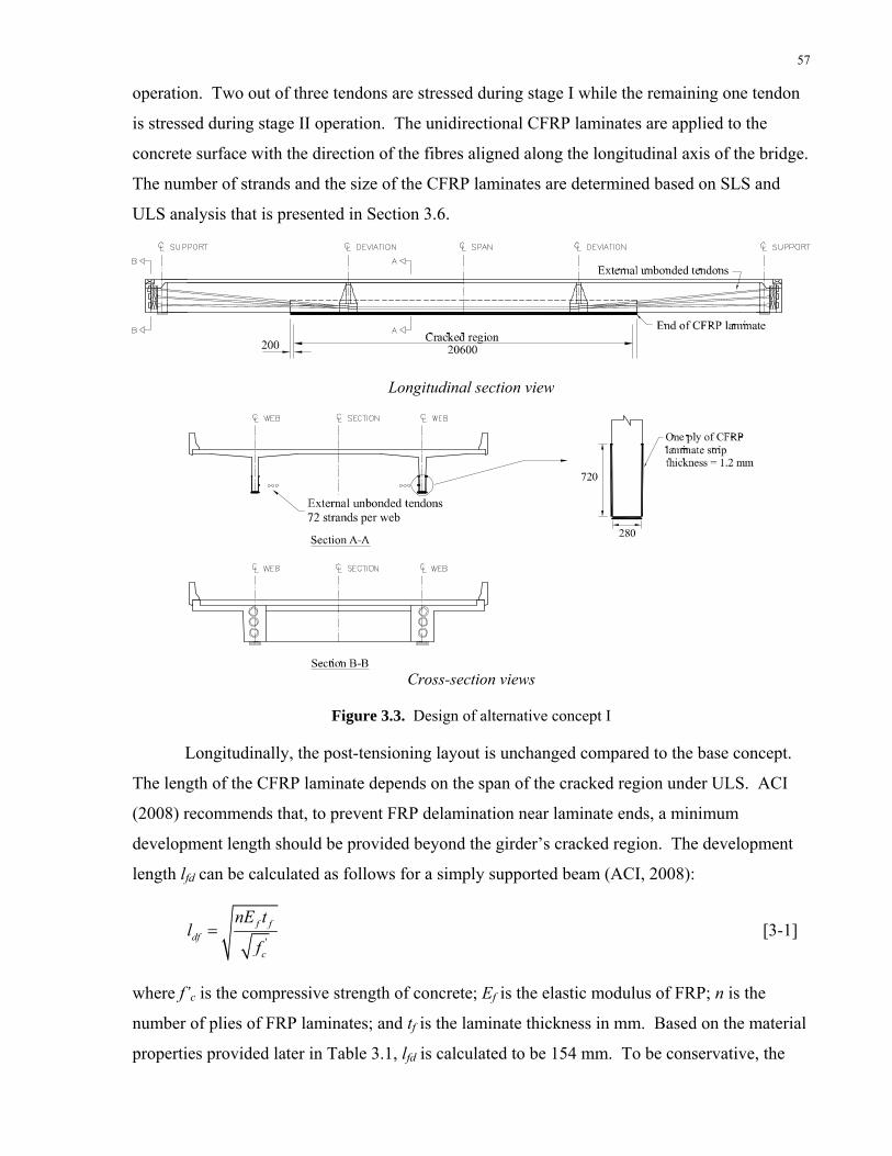
57

operation. Two out of three tendons are stressed during stage I while the remaining one tendon

is stressed during stage II operation. The unidirectional CFRP laminates are applied to the

concrete surface with the direction of the fibres aligned along the longitudinal axis of the bridge.

The number of strands and the size of the CFRP laminates are determined based on SLS and

ULS analysis that is presented in Section 3.6.

Longitudinal section view

Cross-section views

Figure 3.3. Design of alternative concept I

Longitudinally, the post-tensioning layout is unchanged compared to the base concept.

The length of the CFRP laminate depends on the span of the cracked region under ULS. ACI

(2008) recommends that, to prevent FRP delamination near laminate ends, a minimum

development length should be provided beyond the girder’s cracked region. The development

length lfd can be calculated as follows for a simply supported beam (ACI, 2008):

'

f fdf

c

nE tl

f= [3-1]

where f’c is the compressive strength of concrete; Ef is the elastic modulus of FRP; n is the

number of plies of FRP laminates; and tf is the laminate thickness in mm. Based on the material

properties provided later in Table 3.1, lfd is calculated to be 154 mm. To be conservative, the

58

CFRP strips are extended 200 mm beyond the cracked region. More details on the calculation

of cracked region can be found in Section 3.6.3.


The material properties assumed for the design in this Chapter are summarized in Table

3.1. The properties of concrete, mild steel and prestressing steel are same as those used in the

base concept. The CFRP properties are based on the Sika CarboDur composite system (Sika,

2009).

Table 3.1. Material properties


Concrete Specified compressive strength: Ec = 36 300 MPa f'c = 70 MPa Cracking strength: fcr = 3.35 MPa

Reinforcement Yield strength: Es = 200 000 MPa fy = 400 MPa Prestressing steel Specified tensile strength: Ep = 200 000 MPa Size 15 (Astrand = 140 mm2) fpu = 1860 MPa Yield strength: fpy = 0.90 fpu = 1674 MPa

CFRP Tensile strength: Ef = 165 000 MPa Sika CarboDur composite system ffu = 2800 MPa Type S plate (thickness = 1.4mm) (breaking strain εfu = 0.017)

The behaviour of CFRP composites is very different from steel. Like other types of FRP

materials, CFRP does not yield in tension; instead, the composite exhibits a linear stress-strain

relationship up to its brittle failure. The behaviour of CFRP in tension is contrasted to mild steel

in Figure 3.4. As shown by the stress-strain curves, the CFRP has a much higher ultimate

strength, but does not have the ductility that mild steel has. Consequently, the design of CFRP

reinforced structures needs to ensure that the brittle failure of CFRP does not occur.

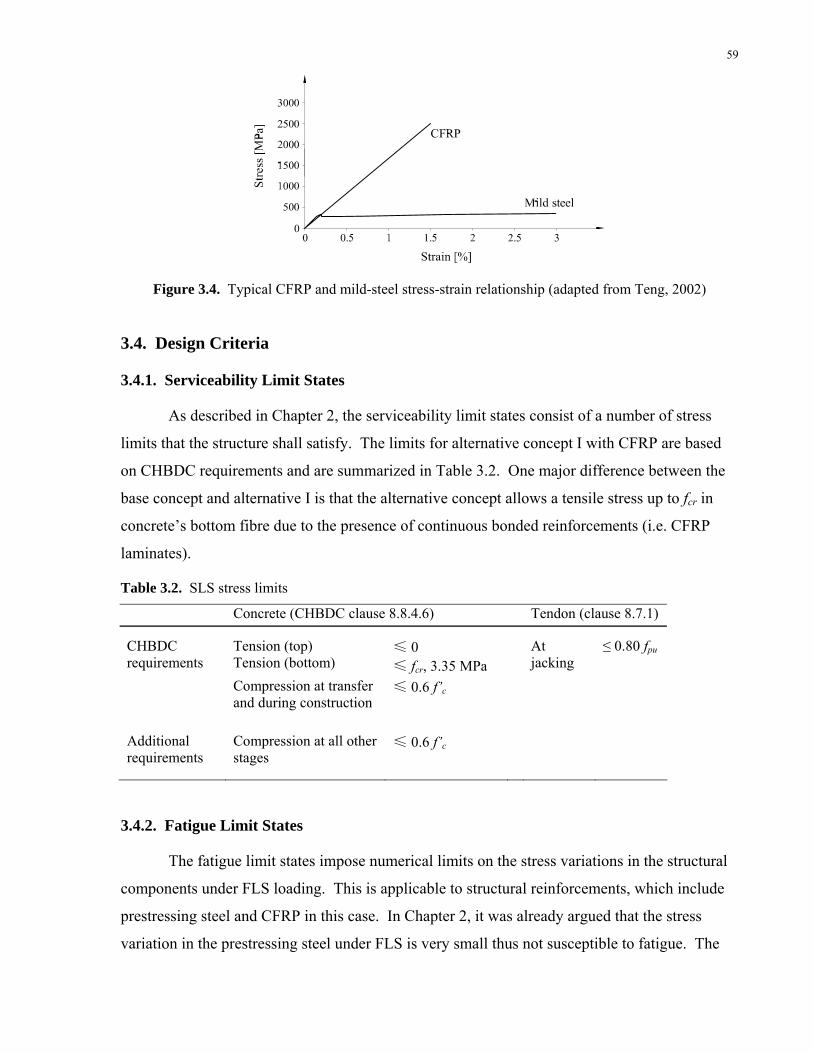
59

Figure 3.4. Typical CFRP and mild-steel stress-strain relationship (adapted from Teng, 2002)



As described in Chapter 2, the serviceability limit states consist of a number of stress

limits that the structure shall satisfy. The limits for alternative concept I with CFRP are based

on CHBDC requirements and are summarized in Table 3.2. One major difference between the

base concept and alternative I is that the alternative concept allows a tensile stress up to fcr in

concrete’s bottom fibre due to the presence of continuous bonded reinforcements (i.e. CFRP

laminates).

Table 3.2. SLS stress limits

Concrete (CHBDC clause 8.8.4.6) Tendon (clause 8.7.1)

Tension (top) Tension (bottom)

≤ 0 ≤ fcr, 3.35 MPa

At jacking

≤ 0.80 fpuCHBDC requirements


≤ 0.6 f’c

Additional requirements


≤ 0.6 f’c

3.4.2. Fatigue Limit States

The fatigue limit states impose numerical limits on the stress variations in the structural

components under FLS loading. This is applicable to structural reinforcements, which include

prestressing steel and CFRP in this case. In Chapter 2, it was already argued that the stress

variation in the prestressing steel under FLS is very small thus not susceptible to fatigue. The

60

FLS evaluation in the chapter thus focuses on the behaviour of CFRP. Because CHBDC does

not provide a specific allowable stress range for CFRP, the evaluation adopts the

recommendation from ACI (2008), which suggests that the sustained plus cyclic stress in the

CFRP should be limited to 0.55 ffu.


Under ultimate limit states, the structure’s factored resistance should be greater than or

equal to the factored load effect.

The structure’s factored resistance is governed by the controlling failure mode. In a

conventional reinforced concrete structure, a flexural member often fails by crushing of concrete

or yielding of reinforcements followed by concrete crushing (ACI, 2008). For a FRP reinforced

structure, the design needs to consider additional failure modes involving the failure of FRP,

such as (ACI, 2008):

Rupture of FRP laminate;

Delamination of concrete cover;

Debonding of FRP from concrete.

The rupture of FRP is assumed to occur when the strain in the FRP exceeds the ultimate

breaking strain (εfu) specified by the manufacturer. For the FRP system employed in this

chapter, the breaking strain is 0.017 as given in Table 3.1.

Delamination of concrete cover refers to a failure mode by which the FRP laminate

separates from the concrete substrate near the end of the laminate, as shown in Figure 3.5a (ACI,

2008). Some believes that this failure mode is caused by the concentrated stress resulted from

the sudden termination of the FRP laminate (Teng, 2002). Once crack forms, it propagates to

steel reinforcements, which acts as a “bond breaker” and leads the crack to progress horizontally

(ACI, 2008; Teng, 2002). Subsequently, the concrete cover pulls away. This failure mode can

in most parts be avoided by proper detailing of the FRP termination, such as using an anchorage

or providing enough development length (ACI, 2008). The recommended development length

for the sample design was already discussed in the brief design description in Section 3.2.

FRP debonding refers to a failure mode that occurs away from FRP termination. Under

this failure mode, debonding is initiated by intermediate flexural and shear cracks and advances

toward the end of the FRP laminate. The debonding may occur in either the adhesive layer or

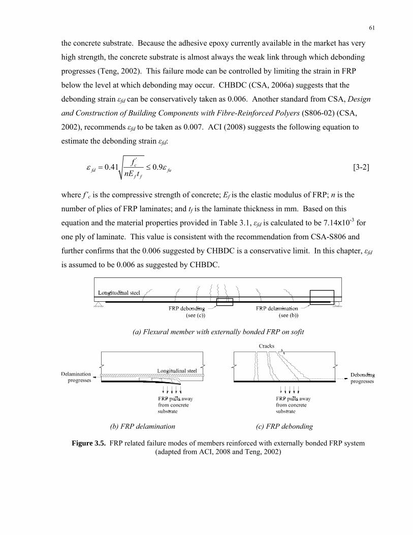
61

the concrete substrate. Because the adhesive epoxy currently available in the market has very

high strength, the concrete substrate is almost always the weak link through which debonding

progresses (Teng, 2002). This failure mode can be controlled by limiting the strain in FRP

below the level at which debonding may occur. CHBDC (CSA, 2006a) suggests that the

debonding strain εfd can be conservatively taken as 0.006. Another standard from CSA, Design

and Construction of Building Components with Fibre-Reinforced Polyers (S806-02) (CSA,

2002), recommends εfd to be taken as 0.007. ACI (2008) suggests the following equation to

estimate the debonding strain εfd:

'

0.41 0.9cfd fu

f f

fnE t

ε ε= ≤ [3-2]

where f’c is the compressive strength of concrete; Ef is the elastic modulus of FRP; n is the

number of plies of FRP laminates; and tf is the laminate thickness in mm. Based on this

equation and the material properties provided in Table 3.1, εfd is calculated to be 7.14x10-3 for

one ply of laminate. This value is consistent with the recommendation from CSA-S806 and

further confirms that the 0.006 suggested by CHBDC is a conservative limit. In this chapter, εfd

is assumed to be 0.006 as suggested by CHBDC.

(a) Flexural member with externally bonded FRP on sofit

(b) FRP delamination (c) FRP debonding

Figure 3.5. FRP related failure modes of members reinforced with externally bonded FRP system (adapted from ACI, 2008 and Teng, 2002)

62

As indicated in the above discussion, FRP rupture cannot occur if the strain in FRP is

kept below the debonding strain εfd, which is only about 35% of the breaking strain. The

delamination of concrete cover can also be mitigated by means of installing anchorages or

providing enough development length. Therefore, FRP debonding is governing among the three

failure modes associated with FRP.

3.5. Load Combinations and Associated Prestress Parameters

The eight load combinations (four for SLS and four for ULS) and corresponding load

factors used Chapter 2 will also be applied to the design of the alternative concept in this

Chapter. Their descriptions can be found in Section 2.4.4 and Table 2.5, and are not repeated

here. The only additional load combination in this chapter is FLS 1 for the fatigue limit states.

The load factors associated with FLS 1 is summarized in Table 3.3. One important difference

between FLS 1 and the SLS and ULS load cases is that live load under FLS consists of one CL-

W truck only, placed at the centre of one travelled lane. This change reduces the overall live

load demand on the girder.

Table 3.3. Fatigue limit states load combination

Load Factor - α Case Combination DL SDL - B SDL - WS LL P

FLS 1 DL + SDL + P1∞ + P2∞ + LL* 1 1 1 1 1

Note: Live load consists of one truck only, placed at the centre of one travelled lane (CSA, 2006a)

An important parameter that is associated with the load combinations is the stress in

prestressing tendons. In Chapter 2, the prestress level was calculated for each load combination

based on the stage of construction each combination corresponds to and the associated loading.

However, there is some uncertainty associated with the prestress losses, coming from both short

and long-term losses. Short-term losses due to anchor set and friction are dependent on the

selection of hardware system and somewhat on how the construction is carried out on site. As a

result, a designer can only estimate these losses during the design phase based on

recommendations from various standards and manufactures’ specifications. Uncertainty in

long-term losses mainly comes from: 1) At the design stage, it is somewhat difficult to predict

accurately the time between stage I and stage II post-tensioning; 2) Even with an accurate

prediction of the time between two stages of post-tensioning operation, there is some inherent

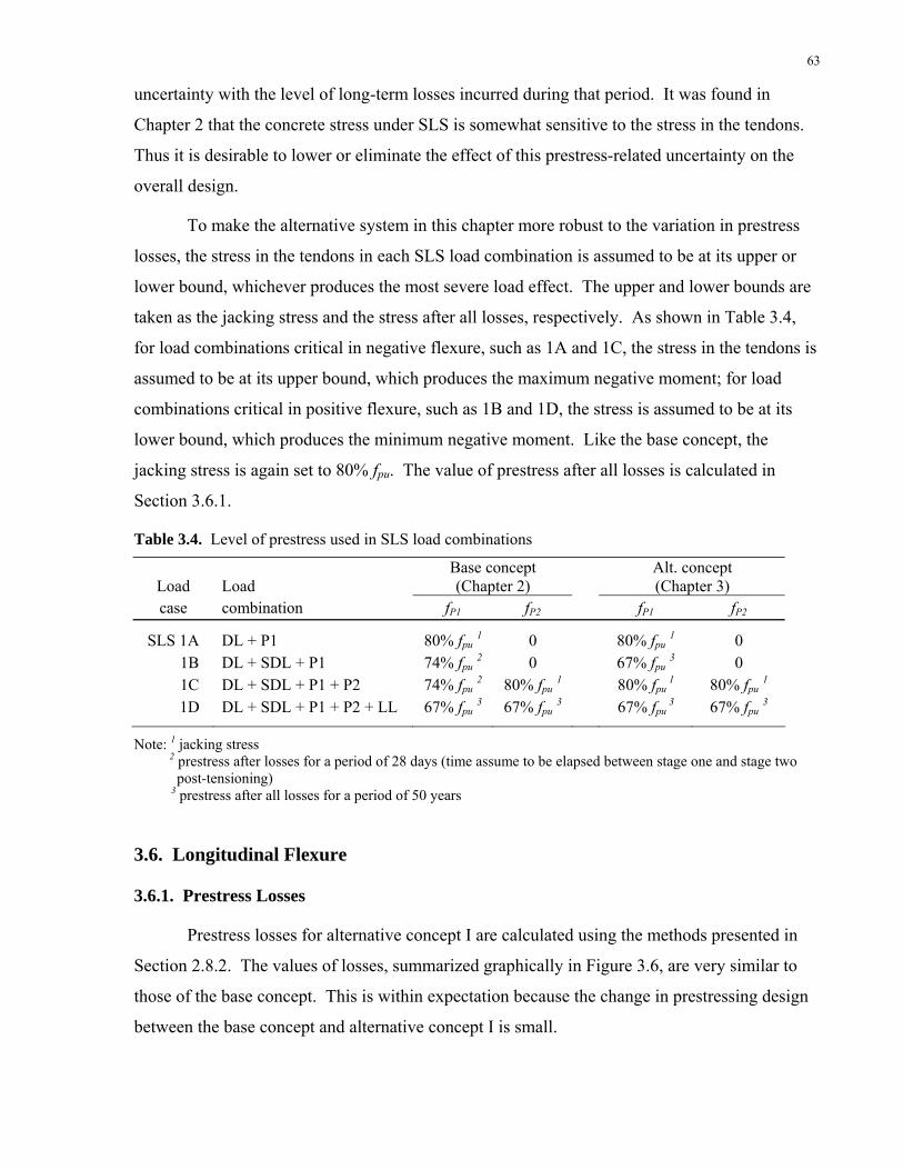
63

uncertainty with the level of long-term losses incurred during that period. It was found in

Chapter 2 that the concrete stress under SLS is somewhat sensitive to the stress in the tendons.

Thus it is desirable to lower or eliminate the effect of this prestress-related uncertainty on the

overall design.

To make the alternative system in this chapter more robust to the variation in prestress

losses, the stress in the tendons in each SLS load combination is assumed to be at its upper or

lower bound, whichever produces the most severe load effect. The upper and lower bounds are

taken as the jacking stress and the stress after all losses, respectively. As shown in Table 3.4,

for load combinations critical in negative flexure, such as 1A and 1C, the stress in the tendons is

assumed to be at its upper bound, which produces the maximum negative moment; for load

combinations critical in positive flexure, such as 1B and 1D, the stress is assumed to be at its

lower bound, which produces the minimum negative moment. Like the base concept, the

jacking stress is again set to 80% fpu. The value of prestress after all losses is calculated in

Section 3.6.1.

Table 3.4. Level of prestress used in SLS load combinations

Load Load Base concept (Chapter 2)

Alt. concept (Chapter 3)

case combination fP1 fP2 fP1 fP2

SLS 1A DL + P1 80% fpu 1 0 80% fpu 1 0 1B DL + SDL + P1 74% fpu 2 0 67% fpu 3 0 1C DL + SDL + P1 + P2 74% fpu 2 80% fpu 1 80% fpu

1 80% fpu 1 1D DL + SDL + P1 + P2 + LL 67% fpu 3 67% fpu 3 67% fpu

3 67% fpu 3

Note: 1 jacking stress 2 prestress after losses for a period of 28 days (time assume to be elapsed between stage one and stage two post-tensioning)

3 prestress after all losses for a period of 50 years


3.6.1. Prestress Losses

Prestress losses for alternative concept I are calculated using the methods presented in

Section 2.8.2. The values of losses, summarized graphically in Figure 3.6, are very similar to

those of the base concept. This is within expectation because the change in prestressing design

between the base concept and alternative concept I is small.

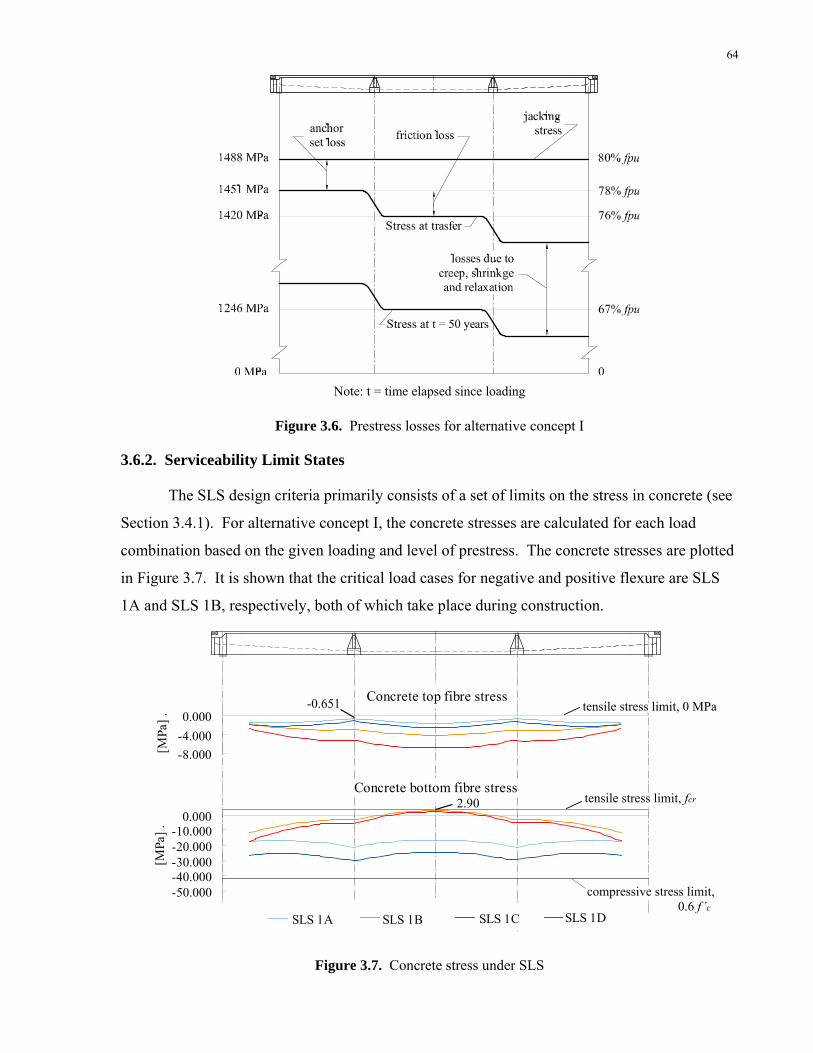
64

Note: t = time elapsed since loading

Figure 3.6. Prestress losses for alternative concept I


The SLS design criteria primarily consists of a set of limits on the stress in concrete (see

Section 3.4.1). For alternative concept I, the concrete stresses are calculated for each load

combination based on the given loading and level of prestress. The concrete stresses are plotted

in Figure 3.7. It is shown that the critical load cases for negative and positive flexure are SLS

1A and SLS 1B, respectively, both of which take place during construction.


-8.000-4.0000.000

[MPa

].

Concrete bottom fibre stress

-50.000-40.000-30.000-20.000-10.000

0.000

[MPa

].

SLS 1A SLS 1B SLS 1C SLS 1D

tensile stress limit, 0 MPa

tensile stress limit, fcr

-0.651

2.90

compressive stress limit,0.6 f ’c


65

Because the above concrete stresses are calculated using the upper and lower bound

values for the tendon stress, they are less sensitive to the variations in PT losses compared to the

base concept. For example, the tensile stress of 2.90 MPa at the concrete bottom fibre under

SLS 1B is calculated by assuming that stage I tendons have incurred all short and long term

losses just prior to the stressing of stage II tendons. In reality, stage I tendons by then has only

lost a portion of all the long term losses. Thus the concrete stress is likely lower than the

calculated 2.90 MPa and further below the tensile stress limit fcr.


The structural response under ultimate limit states are evaluated under the four load

combinations described earlier. Figure 3.8 plots the total moment under the four load

combinations, which is the sum of moments due to prestressing and applied gravity loads.

These load cases can be grouped into two categories: negative-flexure-critical cases such as

ULS 1A and 1C and positive-flexure-critical cases such as ULS 1B and 1D.

-12000-8000-4000

040008000

12000

ULS 1AULS 1B

ULS 1CULS 1D

Mtot(MQ+MP)

[kN-m]

Negative-flexure-critical load combinations:Positive-flexure-critical load combinations:

Figure 3.8. Moment diagrams under ULS load combinations

For the negative-flexure-critical cases, the prestressing forces dominate over gravity

loads, resulting in overall negative flexure in the system. The concrete stresses under ULS 1A

and 1C are calculated and shown in Figure 3.9. Although the concrete top fibre stress goes

slightly into tension, it still remains below the cracking stress fcr under both ULS 1A and 1C. At

the same time, the concrete bottom fibre stress is kept below 0.6 f’c. These two observations

suggest that concrete is still linear elastic under ULS 1A and 1C, hence confirm that the

structural capacity is adequate under these two load combinations.

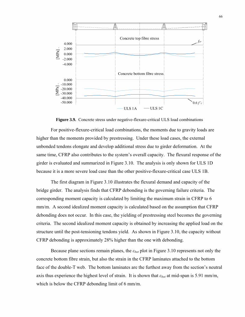
66


-4.000-2.0000.0002.0004.000

[MPa

].


-50.000-40.000-30.000-20.000-10.000

0.000

[MPa

].

ULS 1A ULS 1C

fcr

0.6 f’c

Figure 3.9. Concrete stress under negative-flexure-critical ULS load combinations

For positive-flexure-critical load combinations, the moments due to gravity loads are

higher than the moments provided by prestressing. Under these load cases, the external

unbonded tendons elongate and develop additional stress due to girder deformation. At the

same time, CFRP also contributes to the system’s overall capacity. The flexural response of the

girder is evaluated and summarized in Figure 3.10. The analysis is only shown for ULS 1D

because it is a more severe load case than the other positive-flexure-critical case ULS 1B.

The first diagram in Figure 3.10 illustrates the flexural demand and capacity of the

bridge girder. The analysis finds that CFRP debonding is the governing failure criteria. The

corresponding moment capacity is calculated by limiting the maximum strain in CFRP to 6

mm/m. A second idealized moment capacity is calculated based on the assumption that CFRP

debonding does not occur. In this case, the yielding of prestressing steel becomes the governing

criteria. The second idealized moment capacity is obtained by increasing the applied load on the

structure until the post-tensioning tendons yield. As shown in Figure 3.10, the capacity without

CFRP debonding is approximately 28% higher than the one with debonding.

Because plane sections remain planes, the εbot plot in Figure 3.10 represents not only the

concrete bottom fibre strain, but also the strain in the CFRP laminates attached to the bottom

face of the double-T web. The bottom laminates are the furthest away from the section’s neutral

axis thus experience the highest level of strain. It is shown that εbot at mid-span is 5.91 mm/m,

which is below the CFRP debonding limit of 6 mm/m.

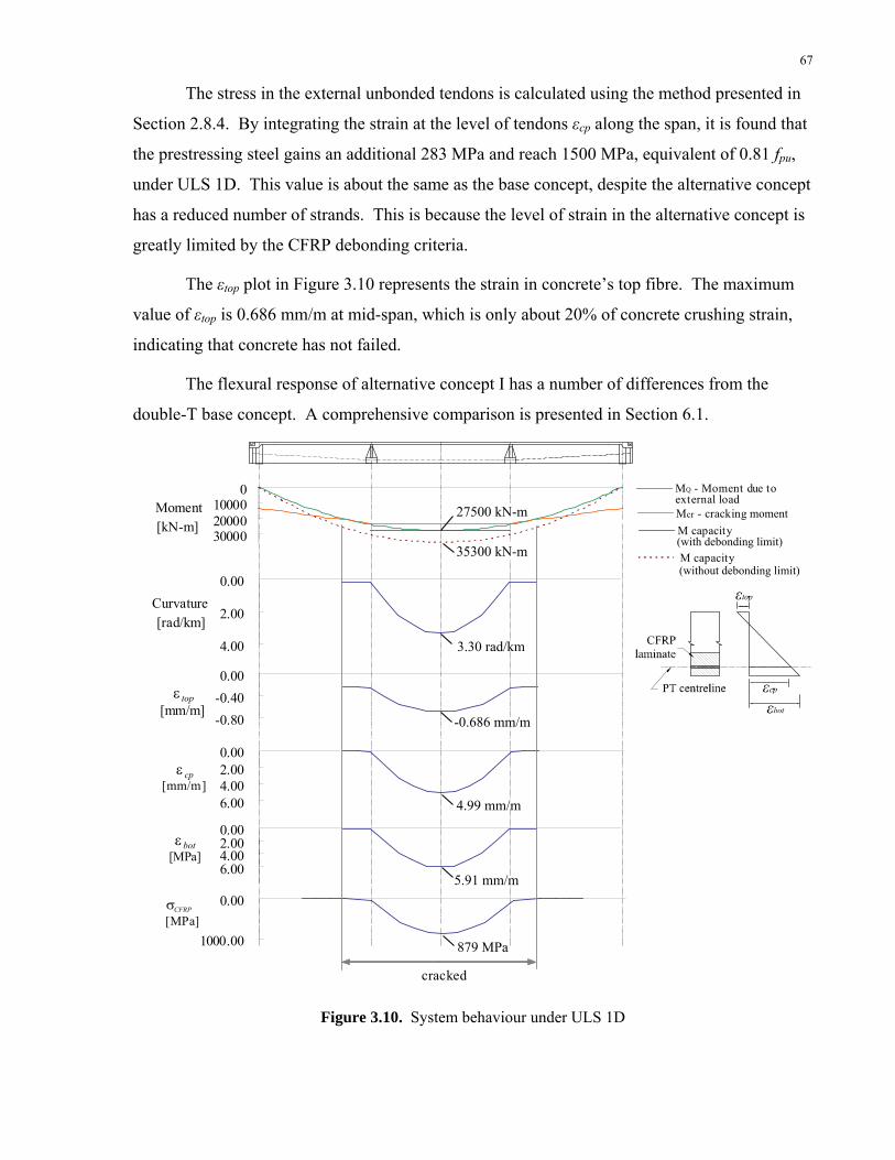
67

The stress in the external unbonded tendons is calculated using the method presented in

Section 2.8.4. By integrating the strain at the level of tendons εcp along the span, it is found that

the prestressing steel gains an additional 283 MPa and reach 1500 MPa, equivalent of 0.81 fpu,

under ULS 1D. This value is about the same as the base concept, despite the alternative concept

has a reduced number of strands. This is because the level of strain in the alternative concept is

greatly limited by the CFRP debonding criteria.

The εtop plot in Figure 3.10 represents the strain in concrete’s top fibre. The maximum

value of εtop is 0.686 mm/m at mid-span, which is only about 20% of concrete crushing strain,

indicating that concrete has not failed.

The flexural response of alternative concept I has a number of differences from the

double-T base concept. A comprehensive comparison is presented in Section 6.1.

0.002.004.006.00

[MPa]

0.00

1000.00[MPa]

0100002000030000

Moment[kN-m]

MQ - Moment due toexternal loadMcr - cracking moment

M capacity

M capacity

(without debonding limit)

(with debonding limit)

-0.80-0.400.00

[mm/m]

0.00

2.00

4.00

Curvature[rad/km]

0.002.004.006.00

[mm/m]

cracked

topε

σ

botε

cpε

35300 kN-m

27500 kN-m

3.30 rad/km

-0.686 mm/m

4.99 mm/m

5.91 mm/m

879 MPa

CFRP

Figure 3.10. System behaviour under ULS 1D

68


Under FLS, the stress in CFRP laminates due to sustained and cyclic load needs to be

limited under 55% of the CFRP’s ultimate strength ffu. Given that ffu is 2800 MPa, the FLS

stress limit on CFRP equals 1540 MPa. In the ULS analysis from the previous section, it was

found that the maximum stress in CFRP is 879 MPa under ULS 1D. As shown in the schematic

comparison of ULS 1D and FLS 1 loading (Figure 3.13), flexural demand under ULS is much

higher than under FLS. This is due to: 1) The load factors under ULS 1D are higher than FLS 1;

2) Live load under ULS requires multiple design lanes to be loaded while live load under FLS

consists of only one truck placed in one traffic lane. Because load is lower under FLS 1, the

stress in CFRP under FLS 1 is expected to be less than 879 MPa, which is the CFRP stress

under ULS 1D. This assures that the CFRP stress under FLS is lower than 0.55 ffu, or 1540 MPa.

Figure 3.11. Schematic diagrams of moments under load combination ULS 1D and FLS 1

3.7. Shear Design

The shear resistance of the alternative concept comes from stirrups, deviated prestressing

tendons and concrete. CFRP laminates does not contribute to shear resistance because the fibres

are aligned along the longitudinal axis of the bridge. Same as the base concept, the shear design

of the alternative concept follows the method prescribed by CHBDC clause 8.9. The final

design is shown in Figure 3.12.

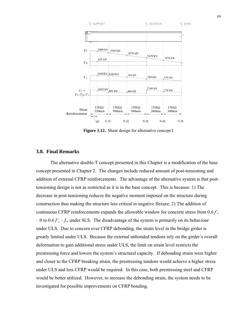
69

Figure 3.12. Shear design for alternative concept I

3.8. Final Remarks

The alternative double-T concept presented in this Chapter is a modification of the base

concept presented in Chapter 2. The changes include reduced amount of post-tensioning and

addition of external CFRP reinforcements. The advantage of the alternative system is that post-

tensioning design is not as restricted as it is in the base concept. This is because: 1) The

decrease in post-tensioning reduces the negative moment imposed on the structure during

construction thus making the structure less critical in negative flexure; 2) The addition of

continuous CFRP reinforcements expands the allowable window for concrete stress from 0.6 f’c

– 0 to 0.6 f’c – fcr under SLS. The disadvantage of the system is primarily on its behaviour

under ULS. Due to concern over CFRP debonding, the strain level in the bridge girder is

greatly limited under ULS. Because the external unbonded tendons rely on the girder’s overall

deformation to gain additional stress under ULS, the limit on strain level restricts the

prestressing force and lowers the system’s structural capacity. If debonding strain were higher

and closer to the CFRP breaking strain, the prestressing tendons would achieve a higher stress

under ULS and less CFRP would be required. In this case, both prestressing steel and CFRP

would be better utilized. However, to increase the debonding strain, the system needs to be

investigated for possible improvements on CFRP bonding.

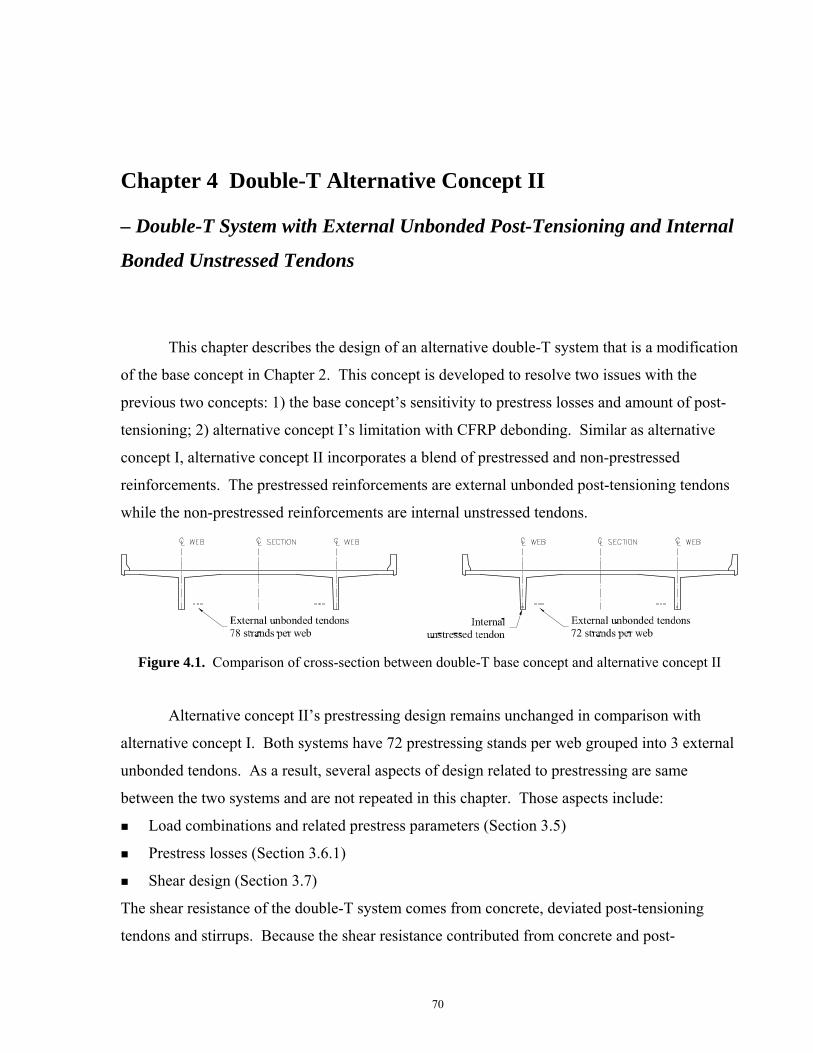
Chapter 4 Double-T Alternative Concept II

– Double-T System with External Unbonded Post-Tensioning and Internal

Bonded Unstressed Tendons

This chapter describes the design of an alternative double-T system that is a modification

of the base concept in Chapter 2. This concept is developed to resolve two issues with the

previous two concepts: 1) the base concept’s sensitivity to prestress losses and amount of post-

tensioning; 2) alternative concept I’s limitation with CFRP debonding. Similar as alternative

concept I, alternative concept II incorporates a blend of prestressed and non-prestressed

reinforcements. The prestressed reinforcements are external unbonded post-tensioning tendons

while the non-prestressed reinforcements are internal unstressed tendons.

Figure 4.1. Comparison of cross-section between double-T base concept and alternative concept II

Alternative concept II’s prestressing design remains unchanged in comparison with

alternative concept I. Both systems have 72 prestressing stands per web grouped into 3 external

unbonded tendons. As a result, several aspects of design related to prestressing are same

between the two systems and are not repeated in this chapter. Those aspects include:

Load combinations and related prestress parameters (Section 3.5)

Prestress losses (Section 3.6.1)

Shear design (Section 3.7)

The shear resistance of the double-T system comes from concrete, deviated post-tensioning

tendons and stirrups. Because the shear resistance contributed from concrete and post-

70

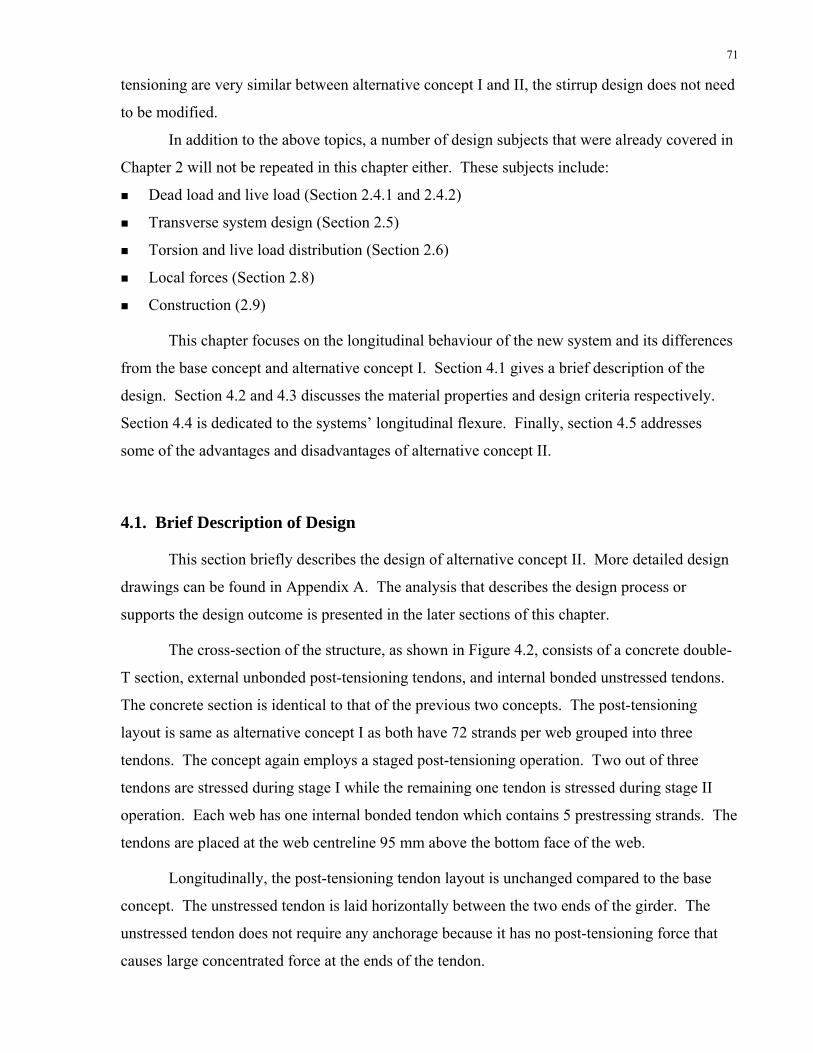
71

tensioning are very similar between alternative concept I and II, the stirrup design does not need

to be modified.

In addition to the above topics, a number of design subjects that were already covered in

Chapter 2 will not be repeated in this chapter either. These subjects include:

Dead load and live load (Section 2.4.1 and 2.4.2)

Transverse system design (Section 2.5)

Torsion and live load distribution (Section 2.6)

Local forces (Section 2.8)

Construction (2.9)

This chapter focuses on the longitudinal behaviour of the new system and its differences

from the base concept and alternative concept I. Section 4.1 gives a brief description of the

design. Section 4.2 and 4.3 discusses the material properties and design criteria respectively.

Section 4.4 is dedicated to the systems’ longitudinal flexure. Finally, section 4.5 addresses

some of the advantages and disadvantages of alternative concept II.


This section briefly describes the design of alternative concept II. More detailed design

drawings can be found in Appendix A. The analysis that describes the design process or

supports the design outcome is presented in the later sections of this chapter.

The cross-section of the structure, as shown in Figure 4.2, consists of a concrete double-

T section, external unbonded post-tensioning tendons, and internal bonded unstressed tendons.

The concrete section is identical to that of the previous two concepts. The post-tensioning

layout is same as alternative concept I as both have 72 strands per web grouped into three

tendons. The concept again employs a staged post-tensioning operation. Two out of three

tendons are stressed during stage I while the remaining one tendon is stressed during stage II

operation. Each web has one internal bonded tendon which contains 5 prestressing strands. The

tendons are placed at the web centreline 95 mm above the bottom face of the web.

Longitudinally, the post-tensioning tendon layout is unchanged compared to the base

concept. The unstressed tendon is laid horizontally between the two ends of the girder. The

unstressed tendon does not require any anchorage because it has no post-tensioning force that

causes large concentrated force at the ends of the tendon.

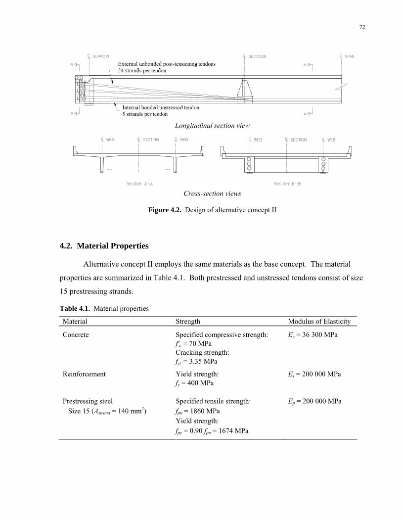
72

Longitudinal section view

Cross-section views

Figure 4.2. Design of alternative concept II


Alternative concept II employs the same materials as the base concept. The material

properties are summarized in Table 4.1. Both prestressed and unstressed tendons consist of size

15 prestressing strands.

Table 4.1. Material properties


Concrete Specified compressive strength: Ec = 36 300 MPa f'c = 70 MPa Cracking strength: fcr = 3.35 MPa

Reinforcement Yield strength: Es = 200 000 MPa fy = 400 MPa Prestressing steel Specified tensile strength: Ep = 200 000 MPa Size 15 (Astrand = 140 mm2) fpu = 1860 MPa Yield strength: fpy = 0.90 fpu = 1674 MPa

73



The serviceability limit states consist of a set of stress limits for concrete and

prestressing steel, which is summarized in Table 4.2. The stress limits on concrete and post-

tensioning tendons are same as those for alternative concept I. The tensile stress limit on

concrete is at fcr because the system has continuous bonded tendons along the span. For the

prestressing steel in the unstressed tendons, the stress under SLS is limited to 240 MPa. This

criterion, which is adapted from CHBDC requirements, is a mean of controlling the overall

deformation and size of cracks in concrete under SLS.

Table 4.2. SLS stress limits

Concrete (CHBDC clause 8.8.4.6)

Prestressing steel (CHBDC clause 8.7.1)

Post-tensioned tendons Tension (top) Tension (bottom)

≤ 0 MPa ≤ fcr, 3.35 MPa

At jacking ≤ 0.80 fpu CHBDC requirements


≤ 0.6 f’c

Unstressed tendons Additional requirements


≤ 0.6 f’c Tension ≤ 240 MPa


According to CHBDC, the stress variation in tendons should be limited under 125 MPa

under FLS. In Chapter 2, it was already argued that the stress variation in the post-tensioned

tendon is very small thus not susceptible to fatigue. The prestressing steel in the unstressed

tendon on the other hand will need to be checked against the stress limit under FLS.


Under ultimate limit states, the structure’s factored resistance should be greater than or

equal to the factored load effect. The factored resistance, as discussed in Chapter 2, will be

controlled by the failure mode of either concrete crushing or the yielding of external unbonded

post-tensioning tendons.

74



Under SLS, the concrete stress depends on the loading and the prestress level under each

load combination. Because alternative concept I and II share the same loading and prestress

design, their concrete stresses under SLS also work out to be the same. The concrete stresses,

shown in Figure 4.3, are calculated based on the prestressing stress’s upper and lower bounds as

discussed in Chapter 3. For a more detailed discussion on level of prestressing and concrete

stresses under SLS, the reader can refer to Section 3.5 and Section 3.6.2.


-8.000-4.0000.000

[MPa

].


-50.000-40.000-30.000-20.000-10.000

0.000

[MPa

].

SLS 1A SLS 1B SLS 1C SLS 1D

tensile stress limit, 0 MPa

tensile stress limit, fcr

-0.651

2.90

compressive stress limit,0.6 f ’c


The other SLS design criterion involves limiting the tensile stress in the internal

unstressed tendons under 240 MPa. This is a mean of controlling the overall girder deformation

and the size of cracks and segmental joint opening. This criterion only needs to be checked for

positive-flexure-critical load under which the unstressed tendon may be in tension. The external

loads and state of stress in the concrete section under SLS 1B and 1D are illustrated in Figure

4.4. It should be noted that SLS 1B in Figure 4.4 is evaluated based on a prestress level that is

closer to its true value than the lower bound value used in calculating the curves in Figure 4.3.

The prestress level used in SLS 1B for stage I tendons is the prestress after 28 days, which is

74% fpu. As shown in Figure 4.4, although both systems are critical in positive flexure, only

SLS 1D results in tension in the unstressed tendon. Under SLS 1D, the tensile stress in the

concrete is not likely to cause significant cracking since it is under the value of fcr predicted by

75

CHBDC. However, at a segmental joint where there is no bond between the adjacent two

concrete surfaces, the system needs to rely on the continuous reinforcements to carry the tensile

stress across. Based on the forces produced by the triangular blocks of tensile stresses, it is

determined that 5 strands are required to satisfy the stress limit of 240 MPa. The resulting stress

in the strands under SLS 1D is 234 MPa.

Load combination SLS 1B

Load combination SLS 1D

Figure 4.4. External load and internal forces under load combinations SLS 1B and SLS 1D


The structural response under ultimate limit states are evaluated under load combinations

ULS 1A, 1B, 1C and 1D, which were described in Section 2.4.4 and Table 2.5. Figure 4.5 plots

the total moment under the four combinations, which is the sum of moments due to prestressing

and applied gravity loads. These load cases can be grouped into two categories: negative-

flexure-critical combinations such as ULS 1A and 1C and positive-flexure-critical combinations

such as ULS 1B and 1D.

76

-12000-8000-4000

040008000

12000

ULS 1AULS 1B

ULS 1CULS 1D

Mtot(MQ+MP)

[kN-m]

Negative-flexure-critical load combinations:Positive-flexure-critical load combinations:

Figure 4.5. Moment diagrams under ULS load combinations

Under the negative-flexure-critical load cases 1A and 1C, the system behaves in the

same manner as alternative concept I. As shown in Figure 4.6, concrete stresses remain

approximately within the linear elastic region between 0.6 f’c and fcr. This indicates that the

structural capacity is adequate for the loading under combination ULS 1A and 1C.


-4.000-2.0000.0002.0004.000

[MPa

].


-50.000-40.000-30.000-20.000-10.000

0.000

[MPa

].

ULS 1A ULS 1C

fcr

0.6 f ’c

Figure 4.6. Concrete stress under negative-flexure-critical ULS load combinations

For positive-flexure-critical load combinations, the moments due to gravity loads are

higher than the moments provided by prestressing. Under these load cases, the external

unbonded tendons elongate and develop additional stress due to girder deformation. At the

same time, the internal bonded unstressed tendons also contribute to the system’s overall

capacity. The flexural response of the girder is evaluated and summarized in Figure 4.7. The

analysis is only shown for ULS 1D because loading under ULS 1D is more severe than ULS 1B.

77

0.00500.00

1000.001500.00

[MPa]

0100002000030000

Moment[kN-m]

MQ - Moment dueto external loadMcr - crackingmomentM capacity

-1.00-0.500.00

[mm/m]

0.00

2.50

5.00

Curvature[rad/km]

0.002.004.006.00

[mm/m]

topε

σ

cpε

30000 kN-m

27500 kN-m

4.31 rad/km

-0.90 mm/m

6.52 mm/m

1460 MPa

S

Cracked

Figure 4.7. System behaviour under ULS 1D

The above moment diagram shows that the moment capacity of the section is 30000 kN-

m, which is approximately 9% above the maximum demand at mid-span. This capacity is

calculated using the same method as in Chapter 2 for the base concept, where the applied load

on the bridge girder is magnified until the stress in the external unbonded tendons reaches 90%

fpu.

The compressive strain in concrete’s top fibre, represented by εtop, has a maximum of -

0.90 mm/m. This is approximately 30% of the concrete crushing strain, indicating that the

concrete is not close to failure.

The stress in the external unbonded tendons is calculated using the method presented in

Section 2.8.4. By integrating the strain at the level of tendons εcp along the span, it is found that

the prestressing steel gains an additional 286 MPa and reach 1530 MPa, equivalent of 0.82 fpu,

under ULS 1D.

78

The flexural response of alternative concept I has a number of differences from the

double-T base concept and alternative concept I. A comprehensive comparison is presented in

Section 6.1.


It was shown in Section 4.4.1 that the concrete girder remains uncracked under SLS.

Thus under FLS with less loading, the concrete would also remain uncracked. As a result, the

unstressed prestressing strands would experience negligible tensile stress under FLS, thus is not

critical in fatigue.

4.5. Final Remarks

The alternative double-T concept presented in this Chapter is a modification of the base

concept presented in Chapter 2. The changes include reduced amount of post-tensioning and the

addition of unstressed internal tendons. Due to these modifications, alternative concept II’s

post-tensioning design is not as restricted as the base concept. The reduction in post-tensioning

decreases the negative moment imposed on the structure during construction thus making the

structure less critical in negative flexure. The addition of internal unstressed tendon, which is

continuous along the span, expands the allowable window for concrete stress from 0.6 f’c – 0 to

0.6 f’c – fcr under SLS, thus giving the designer more flexibility. When compared to alternative

concept I, alternative concept II is no longer limited by the CFRP debonding strain under ULS.

This allows the system to achieve larger deformation and develop higher stress in the unbonded

tendons under ULS. This is indicative of a more efficient utilization of the unbonded tendons.

Chapter 5 Slab-on-Girder Bridge System with CPCI Girders

This chapter describes some important aspects in the design of a conventional slab-on-

girder bridge system with CPCI girders. CPCI girders are standardized I sections commonly

used in Canada. A sample design is developed using a standard design spreadsheet provided by

Hatch Mott MacDonald Mississauga office. The spreadsheet calculation is included in

Appendix B and not discussed in detail in this chapter. Section 5.1 gives a brief introduction to

the CPCI slab-on-girder type of bridge system. Section 5.2 briefly describes the key features of

the sample design, while Section 5.3 gives a summary of the materials used. Section 5.4 and 5.5

examine live load distribution and deck slab design, which are two important aspects in the

design of slab-on-girder bridges. Finally, Section 5.6 is dedicated to construction related

subjects.

5.1. Introduction

Prestressed concrete I-girder bridges were introduced in the 1950s (Kulka and Lin, 1984).

This type of structural system includes a series of precast and prestressed concrete I-girders with

a cast-in-place concrete top slab. One of the first prominent bridges of this type is the Walnut

Lane Memorial Bridge built in Philadelphia, Pennsylvania in 1950 (Dunker and Rabbat, 1992).

Since then, this type of slab-on-girder bridge gained wide popularity in North America and

became the most used bridge system for short-to-medium span bridges (Kulka and Lin, 1984).

A survey done by Dunker and Rabbat in 1992 indicates that they comprise about 40% of all

prestressed concrete bridges constructed in the United States during the period from 1950 to

1989. Precast pre-tensioned I-girders have traditionally been used for spans up to approximately

50 m (Kulka and Lin, 1984). Nowadays, the range of span can be extended to 75 m by using I-

girders that are spliced together with longitudinal post-tensioning (Lounis et al, 1997).

I-girders are highly standardised in today’s bridge industry (FHWA, 2009). A number

of standard I sections have been developed, such as the Florida Bulb-Tee, AASHTO-PCI Bulb-

79

80

Tee and the CPCI standard I sections (Figure 5.1). The first two types of girders are most often

used in the US, while CPCI girders are commonly used in Canada.

Figure 5.1. Standardized I sections (adapted from Pre-Con, 2004 and FHWA, 2009) Despite the wide application of the slab-on-girder system, this type of bridge has its

inherent shortcomings. The first major shortcoming is its inefficient sharing of live load

between girders. Due to the deck slab’s flexibility, the effect of an applied load on the deck slab

can only propagate to a limited number of girders close to the location of the load. The second

shortcoming of the system comes from the inconvenience and cost associated with the cast-in-

place deck slab. Both subjects will be discussed in more detail in later sections.


A slab-on-CPCI-girder system is developed based on the geometrical requirements

presented in Chapter 1. The design is produced with the aid of a standard design spreadsheet

provided by Hatch Mott MacDonald, Missisauga. Sample pages of the spreadsheet as well as a

more complete set of drawings are included in Appendix B for reference.

As shown in Figure 5.2, the cross-section of the bridge consists of a cast-in-place deck

slab 225 mm in thickness and six prestressed precast CPCI 1900 girders spaced at 2350 mm.

The depth of the girder is 1900 mm and the total depth of the structure is 2175 mm. The

concrete girders are pre-tensioned with internal prestressing strands. The strands are installed in

standardized locations within the girder. For the sample design, each girder is equipped with 50

S13 strands, among which 32 are straight and 18 are deflected. The strand layout is shown in

Figure 5.3.

81

Figure 5.2. Sample design of the Slab-on-CPCI-girder system

Figure 5.3. Pre-tension strand layout (adapted from MTO, 2002)


The properties of the materials used in the sample design are summarized in Table 5.1.

There are two major differences between the materials used in the CPCI system and the double-

82

T systems. First, the CPCI system uses a more conventional 50 MPa concrete while the double-

T systems use 70 MPa concrete. Second, because the current pretensioning industry usually

prefers size 13 prestressing strands, the CPCI system does not employ the size 15 strands that

were used in the double-T systems.

Table 5.1. Material properties for slab-on-CPCI-girder sample design


Concrete Specified compressive strength: 1.5( ' 6900)( / 2300)c c cE f γ= + f'c = 50 MPa Ec = 31 900 MPa Cracking strength: 0.4 ' 2.83MPacr cf f= = Reinforcement Yield strength: Es = 200 000 MPa fy = 400 MPa Prestressing steel Specified tensile strength: Ep = 200 000 MPa Size 13

(Astrand = 99 mm2) fpu = 1860 MPa

Yield strength: fpy = 0.90fpu = 1674 MPa

5.4. Live Load Distribution

When vehicular live load is applied on the deck slab, its influence on each girder is

different. It is important for designers to know how load is distributed among girders, as it is a

governing factor in determining the design load for each girder.

The simplified example in Figure 5.4 (Hassanain, 1998) and the following discussion

describe two extreme cases of live load distribution. The example has a slab-on-girder system

that is idealized as three simply-supported girders connected by a transverse beam at mid-span.

A load P is applied at mid-span of the transverse beam, thus directly on the central girder. On

one extreme, if the transverse beam has no stiffness, the three girders become virtually

disconnected, and all load will be taken by the central girder. In this case, Girder 2 carries the

entire P while Girder 1 and 3 carries no load. On the other extreme, if the transverse beam is

infinitely stiff, all three girders will deflect and share the load equally, and the load distributed to

each girder is P/3. The second case illustrates a more efficient load distribution among girders.

83

Figure 5.4. Load distribution in an idealized beam-on-girder system (adapted from Hassanain, 1998)

In a more realistic case where girders are connected by a deck slab, live load distribution

becomes much more complicated. It depends on many factors, such as span length, the

transverse position of live load, the dimension and location of the diaphragms, and the

transverse and longitudinal bending stiffness of the girder-and-slab composite (CSA, 2006b).

Much research has been done in modeling live load distribution in a slab-on-girder

system using grillage, semi-continuum or finite element methods (CSA, 2006b). The results

from these analysis are used to formulate design equations in standards and codes. These

equations are often simplified from the real situation to include only a limited number of

variables. They are usually used to determine the maximum amount of load distributed to a

girder under the most unfavourable conditions. This load level then becomes the design load for

each girder in the system. The following sections describe some of the load distribution

equations used in North America. The equations are also summarized in Table 5.2.

5.4.1. AASHTO Standard

The AASHTO Standard equations have been used in the United States since the 1930s

(Yousif, 2007). They were only recently replaced by the new AASHTO LRFD specification,

which was first published in 1998.

In the AASHTO Standard, a distribution factor (DF) is defined and applied to one line of

wheel load. The equation for DF takes a simple form of S/D, where S is the girder spacing and

D is a constant that depends on the type of bridge and the number lanes loaded (AASHTO,

1996). For concrete slab on girder bridges, D is 2.13 if only one lane is loaded, and 1.68 if two

or more lanes are loaded.

The S/D formula is relatively easy to apply. However, it disregards the effect of span

length, deck slab, and girder stiffness (Yousif, 2007). It was found to produce overly

84

conservative results in some cases and unconservative results in others (Cai, 2005). Also, this

formula is developed only for bridges with typical geometry, thus not applicable to more

complicated bridges (Yousif, 2007). All these shortcomings of the S/D formula led to the

development of the new load distribution formula, which was introduced in AASHTO LRFD

Bridge Design Specifications in 1998.

5.4.2. AASHTO LRFD Specifications

The AASHTO LRFD Specifications provide a more refined method to calculate live

load distribution than the previous S/D equation. In addition to girder spacing, this formula also

takes into consideration the bridge span, slab thickness, and the longitudinal stiffness of the

cross-section (Yousif, 2007).

The distribution factor, which is also applied to one line of wheel load, is defined as

follows (AASHTO 1998):

0.10.4 0.3

30.064300

g

s

KS SDFL Lt

⎛ ⎞⎛ ⎞ ⎛ ⎞= + ⎜ ⎟⎜ ⎟ ⎜ ⎟⎝ ⎠ ⎝ ⎠ ⎝ ⎠

if one lane is loaded [5-1]

0.10.6 0.2

30.0752900

g

s

KS SDFL Lt

⎛ ⎞⎛ ⎞ ⎛ ⎞= + ⎜ ⎟⎜ ⎟ ⎜ ⎟⎝ ⎠ ⎝ ⎠ ⎝ ⎠

if two or more lanes are loaded [5-2]

where S is girder spacing, L is span length, ts is deck slab thickness and Kg is the longitudinal

stiffness. Kg mainly depends on the girder type, and can be calculated as follows (Yousif, 2007):

( )2g g g gK n I A e= + [5-3]

where n is the ratio between the girder and deck’s Elastic Modulus; Ig and Ag are the moment of

inertia and the cross-sectional area of the girder; and eg is the eccentricity between the girder and

slab’s center of gravity.

The AASHTO LRFD method is more elaborate and is shown to produce more accurate

results than the previous S/D formula (Suksawang, 2007). However it complicates the design

procedure significantly because the new equations require the knowledge of the girder cross-

sectional properties, which are generally unknown prior to the determination of design load. As

a result, the design becomes an iterative process. Research has been done in recent years trying

to simplify the new AASHTO LRFD formulations while not compromising its accuracy (Cai,

2005, Suksawang, 2007, and Yousif, 2007).

85

5.4.3. Canadian Highway Bridge Design Code

The Canadian Highway Bridge Design Code prescribes simplified methods for the

analysis of live load distribution. These methods are based on analysis results from modeling

many structures with the grillage, semi-continuum, and finite element methods (CSA 2006b).

To be analyzed using the simplified methods, the bridge must satisfy certain conditions (CSA

2006a). For a straight slab-on-girder bridge, the conditions include:

a. The deck width is constant;

b. The support conditions can be represented by line support;

c. There should be at least three longitudinal girders with approximately equal flexural

rigidity and spacing;

d. The deck slab overhang should be less than 1.80 m and 60% of the average girder

spacing.

CHBDC prescribes several methods to analyze live load distribution. Each method is

applicable to a specific type of load effect under specific limit states, such as SLS, FLS or ULS.

The following discussion focuses on the method for evaluating the distribution of longitudinal

bending moments in slab-on-girder bridges under ULS and SLS.

The method presented in CHBDC centres at the concept of an amplification factor (Fm),

which is defined as:

,

gm

g avg

MF

M= [5-4]

where Mg,avg is the average moment per girder due to live load if live load were shared equally

among girders, and Mg is the maximum longitudinal moment per girder accounting for unequal

live load distribution (CSA, 2006a). Mg,avg can be calculated from the following equation:

,T L

g avgnM RM

N= [5-5]

where n is the number of design lanes, RL is the multi-lane loading reduction factor, N is the

number of girders, and MT is the maximum moment per design lane due to the two-line axel

load (CSA 2006a).

86

It is shown in equation 5-4 that Fm is a measure of how much the extreme load

distribution deviates from the average distribution. Lower values of Fm indicate less deviation,

thus greater ability of the bridge to transfer load across its width (CSA, 2006b). Figure 5.5

shows an Fm versus span graph developed for slab-on-girder bridges with a lane width of 3.33 m.

The graph indicates that bridges with longer spans and narrower decks have a lower value of Fm,

which is a sign of more even live load distribution.

Figure 5.5. Fm for internal girders in a slab-on-girder bridge system under ULS and SLS (CSA, 2006b)

In design, Fm for slab-on-girder type of bridge can be calculated using the following

formula:

1.051

100

mf

SNFC

Fμ

= ≥⎡ ⎤+⎢ ⎥

⎣ ⎦

[5-6]

where S is the girder spacing. There are two key expressions in the above equation for Fm:

F

F is a “width dimension that characterizes the load distribution for a bridge” (CSA,

2006a). It depends on many factors, including bridge type, highway class, span length,

number of design lanes, and girder position. The concept of F is related to the constant D in

AASHTO Standard’s S/D formulation by the following expression (CSA 2006b):

2 LF nR D= [5-7]

The multiplier of 2 accounts for the fact that the AASHTO formulas are based on one line of

wheel load while CHBDC formulas are associated with the full truck load. The factor n and

RL adjusts the constant to account for the multi-lane loading effect. The values of F are

tabulated in CHBDC.

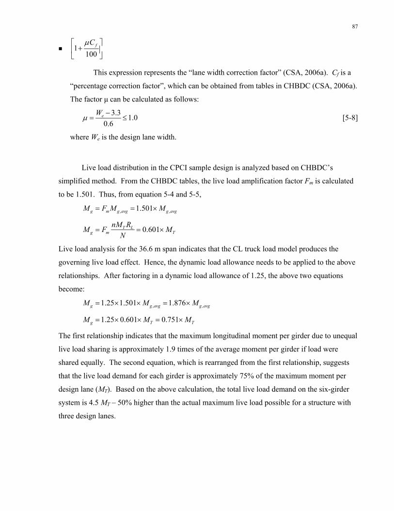
87

1100

fCμ⎡ ⎤+⎢ ⎥

⎣ ⎦

This expression represents the “lane width correction factor” (CSA, 2006a). Cf is a

“percentage correction factor”, which can be obtained from tables in CHBDC (CSA, 2006a).

The factor μ can be calculated as follows:

3.3 1.00.6

eWμ −= ≤ [5-8]

where We is the design lane width.

Live load distribution in the CPCI sample design is analyzed based on CHBDC’s

simplified method. From the CHBDC tables, the live load amplification factor Fm is calculated

to be 1.501. Thus, from equation 5-4 and 5-5,

, ,1.501g m g avg g avgM F M M= = ×

0.601T Lg m T

nM RM F MN

= = ×

Live load analysis for the 36.6 m span indicates that the CL truck load model produces the

governing live load effect. Hence, the dynamic load allowance needs to be applied to the above

relationships. After factoring in a dynamic load allowance of 1.25, the above two equations

become:

, ,1.25 1.501 1.876g g avg g avgM M M= × × = ×

1.25 0.601 0.751g T TM M M= × × = ×

The first relationship indicates that the maximum longitudinal moment per girder due to unequal

live load sharing is approximately 1.9 times of the average moment per girder if load were

shared equally. The second equation, which is rearranged from the first relationship, suggests

that the live load demand for each girder is approximately 75% of the maximum moment per

design lane (MT). Based on the above calculation, the total live load demand on the six-girder

system is 4.5 MT – 50% higher than the actual maximum live load possible for a structure with

three design lanes.

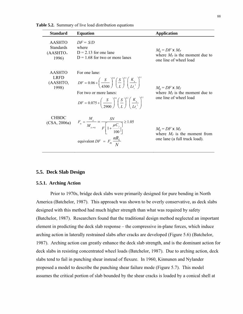
88

Table 5.2. Summary of live load distribution equations

Standard Equation Application

AASHTO Standards

(AASHTO， 1996)

DF = S/D where D = 2.13 for one lane D = 1.68 for two or more lanes

Mg = DF x MT where MT is the moment due to one line of wheel load

AASHTO LRFD

(AASHTO, 1998)

For one lane: 0.10.4 0.3

30.06

4300g

s

KS SDF

L Lt= +

⎛ ⎞⎛ ⎞ ⎛ ⎞⎜ ⎟ ⎜ ⎟ ⎜ ⎟⎝ ⎠ ⎝ ⎠ ⎝ ⎠

For two or more lanes: 0.10.6 0.2

30.075

2900g

s

KS SDF

L Lt= +

⎛ ⎞⎛ ⎞ ⎛ ⎞⎜ ⎟ ⎜ ⎟ ⎜ ⎟⎝ ⎠ ⎝ ⎠ ⎝ ⎠

Mg = DF x MT where MT is the moment due to one line of wheel load

CHBDC (CSA, 2006a)

,

1.051

100

g

mfg avg

M SNF

CMF

μ= ≥

+

=⎡ ⎤⎢ ⎥⎣ ⎦

equivalent LmDF F

nRN

=

Mg = DF x MT where MT is the moment from one lane (a full truck load).

5.5. Deck Slab Design

5.5.1. Arching Action

Prior to 1970s, bridge deck slabs were primarily designed for pure bending in North

America (Batchelor, 1987). This approach was shown to be overly conservative, as deck slabs

designed with this method had much higher strength than what was required by safety

(Batchelor, 1987). Researchers found that the traditional design method neglected an important

element in predicting the deck slab response – the compressive in-plane forces, which induce

arching action in laterally restrained slabs after cracks are developed (Figure 5.6) (Batchelor,

1987). Arching action can greatly enhance the deck slab strength, and is the dominant action for

deck slabs in resisting concentrated wheel loads (Batchelor, 1987). Due to arching action, deck

slabs tend to fail in punching shear instead of flexure. In 1960, Kinnunen and Nylander

proposed a model to describe the punching shear failure mode (Figure 5.7). This model

assumes the critical portion of slab bounded by the shear cracks is loaded by a conical shell at

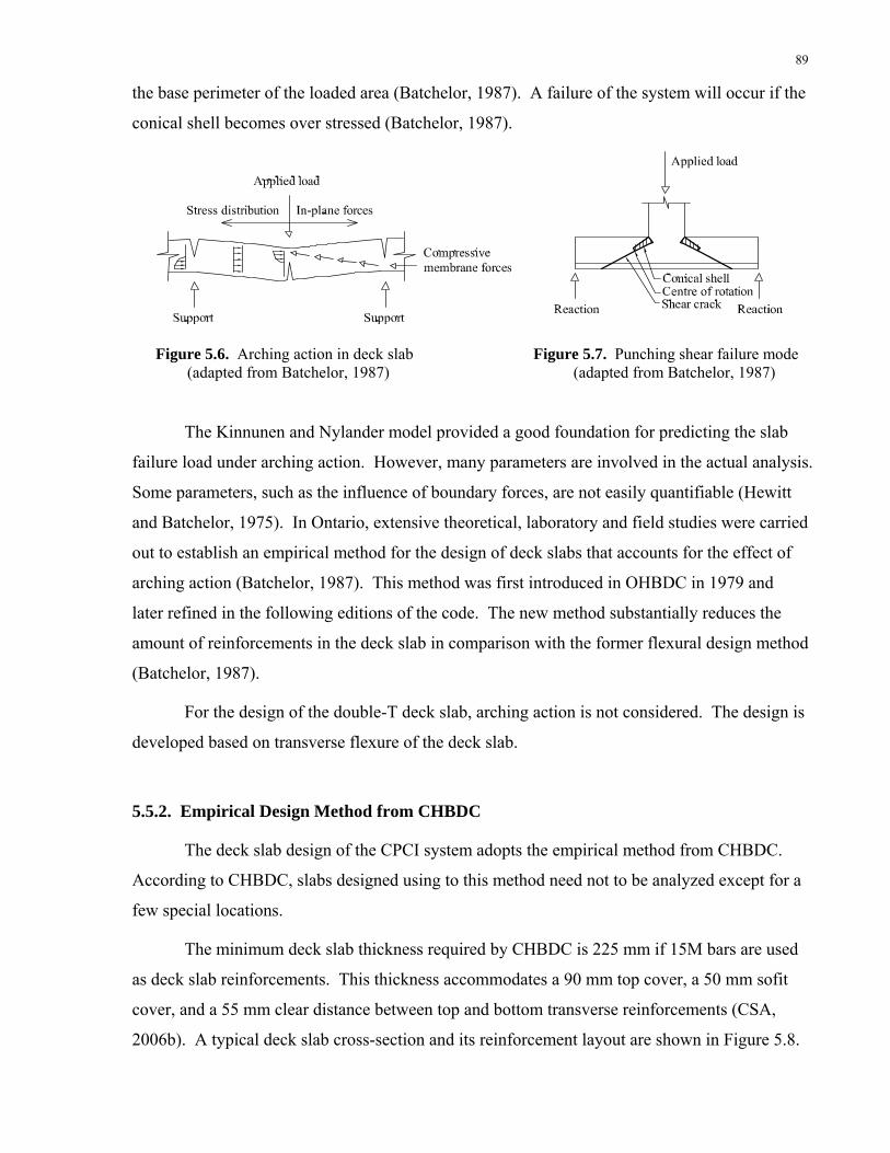
89

the base perimeter of the loaded area (Batchelor, 1987). A failure of the system will occur if the

conical shell becomes over stressed (Batchelor, 1987).

Figure 5.6. Arching action in deck slab Figure 5.7. Punching shear failure mode (adapted from Batchelor, 1987) (adapted from Batchelor, 1987)

The Kinnunen and Nylander model provided a good foundation for predicting the slab

failure load under arching action. However, many parameters are involved in the actual analysis.

Some parameters, such as the influence of boundary forces, are not easily quantifiable (Hewitt

and Batchelor, 1975). In Ontario, extensive theoretical, laboratory and field studies were carried

out to establish an empirical method for the design of deck slabs that accounts for the effect of

arching action (Batchelor, 1987). This method was first introduced in OHBDC in 1979 and

later refined in the following editions of the code. The new method substantially reduces the

amount of reinforcements in the deck slab in comparison with the former flexural design method

(Batchelor, 1987).

For the design of the double-T deck slab, arching action is not considered. The design is

developed based on transverse flexure of the deck slab.

5.5.2. Empirical Design Method from CHBDC

The deck slab design of the CPCI system adopts the empirical method from CHBDC.

According to CHBDC, slabs designed using to this method need not to be analyzed except for a

few special locations.

The minimum deck slab thickness required by CHBDC is 225 mm if 15M bars are used

as deck slab reinforcements. This thickness accommodates a 90 mm top cover, a 50 mm sofit

cover, and a 55 mm clear distance between top and bottom transverse reinforcements (CSA,

2006b). A typical deck slab cross-section and its reinforcement layout are shown in Figure 5.8.

90

Figure 5.8. Typical deck slab design based on CHBDC’s empirical method – cross-section view For a full-depth cast-in-space deck slab, there should be a total of four layers of

reinforcing bars arranged in two orthogonal planes – one plane near the top of the slab and the

other near the bottom. The reinforcement ratio ρ for each layer should be at least 0.003, unless

the deck slab can be proved to behave satisfactorily with less reinforcements. In the latter case,

ρ can be reduced to 0.002. The ratio ρ is defined as:

sAbd

ρ = [5-9]

where b is an arbitrary width, As is the area of reinforcement within the given width b, and d is

the effective depth of concrete. In practice, it is customary to design deck slabs of slab-on-

girder bridges with 15M bars spaced at 300 mm. This translate to a reinforcement ratio slightly

higher than 0.003.

5.6. Construction

5.6.1. CPCI Girder Fabrication

The fabrication of CPCI girders involves first placing and stressing the pretensioning

strands, then laying the reinforcing bars, and finally casting concrete. This process requires

specialized formwork and equipments. The formwork is usually made of steel to maximize its

durability for extended use. Bulkheads as shown in Figure 5.9 are used at ends of the precast

segment to anchor the pre-tensioning strands. Also shown in the figure is a precasting bed made

of steel beams. It serves the purpose of both supporting the cast segment and holding down the

pre-tensioning strands’ deviations. During the casting process, steel side forms are used to form

the side geometry of the CPCI girders. The specialized forms and equipments require high

capital investment. As a result, only a very limited number of suppliers of CPCI girders are

available in Ontario.

91

Figure 5.9. CPCI girder fabrication (photos by P. Gauvreau)

5.6.2. Erection

The superstructure of a single-span CPCI slab-on-girder girder bridge is typically

constructed in the following sequence (Figure 5.10):

1. Erect precast girders;

2. Cast end diaphragms;

3. Place deck slab reinforcements;

4. Cast deck slab once the concrete compressive strength in the diaphragms has reached

the specified value.

The erection of girder is usually done by a crane. The overall construction is relatively standard.

However the speed of construction is often redistricted by the time required to place deck slab

reinforcements and cure the cast-in-place concrete.

Figure 5.10. Typical construction sequence for the superstructure of a slab-on-girder bridge (adapted from WSDOT, 2008)

Bulkhead

Precasting bed

Reinforcing bars

Pretensioning strands

Chapter 6 Evaluation of the Double-T and CPCI Systems

This chapter evaluates the structural efficiency and the material consumption and cost of

the double-T and the CPCI slab-on-girder systems based on the sample designs developed in

Chapter 2 to 5. Section 6.1 examines three alternative double-T systems. Section 6.2 compares

the double-T and the CPCI systems in terms of live load distribution, amount of design load

incurred in the system, and the approaches for deck slab design. Section 6.3 compares the

systems’ material consumption, including the use of concrete, prestressing steel and additional

reinforcements. Finally, Section 6.4 provides a preliminary cost comparison for the systems

developed in this thesis.

6.1. Comparison of Double-T Concepts

The three double-T concepts were developed based on the same concrete cross-section

and transverse design. Differences of the systems lie in the design of their primary longitudinal

reinforcements. While the base concept is reinforced with pure post-tensioning, alternative

concept I and II have a blend of prestressed and non-prestressed primary reinforcements.

The double-T base concept is longitudinally reinforced with pure external unbonded

post-tensioning. The sample design of the double-T base concept is governed by longitudinal

flexure under SLS. It is found in the SLS analysis that the structure is somewhat sensitive to the

level of prestressing losses and the amount of post-tensioning in the system. While the sample

design developed in Chapter 2 is a feasible system responding to the specific geometrical

requirements described in Chapter 1, the double-T base concept’s applicability to different

geometrical conditions may be limited due to the limitation associated with post-tensioning

design.

To improve the double-T system’s adaptability to different geometrical conditions,

alternative concept I is developed with a blend of prestressed and non-prestressed primary

reinforcements. The pretressed reinforcements are again external unbonded post-tensioning

92

93

tendons, while the non-prestressed reinforcements are external CFRP laminates. This

alternative design has two major advantages. First, due to the addition of continuous CFRP

laminate, the concrete stress limit under SLS is increased up to fcr in the bottom fibre, giving the

designer more flexibility. Second, because the system’s positive flexural capacity is

complemented by CFPR, the amount of external post-tensioning can now be reduced, thus

creating less negative flexural demand on the system. For alternative concept I, the concrete

stresses under SLS become less critical and less sensitive to level of prestressing in comparison

with the base concept. The disadvantage of alternative concept I relates to its behaviour under

ULS, where the girder’s overall deformation is restricted by the debonding strain of CFRP

laminate. This restriction lowers the additional stress that can be developed in the unbonded

tendons under ULS and increases the amount of CFRP needed.

A second alternative double-T system is created by replacing the CFRP in alternative

concept I with unstressed internal bonded tendon, which is continuous along the span. The

number of strands provided in the unstressed tendon is governed by a criterion that requires the

stress in the strand to be less than 240 MPa under SLS. This requirement is a mean of

controlling the size of crack and segmental joint opening under SLS. Like alternative concept I,

concrete stresses under SLS is less critical and less sensitive to level of prestressing in

comparison with the base concept. The unbonded tendons under ULS develop slightly higher

stresses than the previous two concepts due to the increase in girder deformation.

Both alternative concept I and II are developed with SLS design criteria that limit the

tensile stress in concrete under fcr. It is possible to increase their SLS concrete tensile stress

limit beyond fcr. However, a thorough examination of cracking needs to be carried out.

Table 6.1 summarizes some of the SLS and ULS characteristics of the double-T systems.

The major difference among the systems under SLS is that the base concept does not allow any

tensile stress in concrete while alternative concept I and II allow up to fcr in concrete’s bottom

fibre where continuous reinforcements are present. Under ULS, although the final stress in the

external unbonded tendons is close among the three concepts, the strain distribution is quite

different. For the base concept, the strain peaks at mid-span at a value of 12.3 mm/m. For the

alternative concepts, the strain diagram displays a more parabolic distribution with a lower

maximum. This indicates that the addition of internal bonded reinforcements help better

distribute strain in the system. The governing design criteria and ULS capacity of the three

systems are also shown in the table. The base concept is governed by concrete tensile stress

94

limit under SLS and display some reserve in ULS capacity. Alternative concept I is governed

by ULS criteria of CFRP debonding. The ULS capacity is calculated based on a CFRP

debonding strain of 6 mm/m, which is a conservative limit suggested by CHBDC (2006b). If

bonding can be improved and made more reliable, the ULS capacity can improve significantly.

Alternative concept II is governed by the SLS stress limit for the internal continuous

prestressing steel. The system’s ULS demand is approximately 92% of its capacity.

Overall, alternative concept II appears to be the most versatile system among the three

concepts. Unlike the base concept which is somewhat constrained by the large amount of post-

tensioning force in the system, alternative concept II can be adapted to other design conditions

by adjusting the amount of post-tensioning based on SLS design criteria and complementing the

ULS capacity with internal unstressed prestressing strands. While there is a certain range of

geometrical conditions that alternative concept II is most suitable for, this system appears to

have a reasonable range of applicability. Alternative concept I with CFRP reinforcements also

has the potential for wider range of application if bonding between CFRP and the double-T

girder can be improved.

Table 6.1. Comparison of double-T systems

Base concept Alternative concept I Alternative concept II

External post-tensioning only External PT + CFRP External PT + unstressed internal tendon

Amt. of external post-tensioning 156 strands 144 strands 144 strands

Amt. of additional reinforcement - CFRP laminate with size of

21m (L)×3.44m (W)×1.2mm (T) 10 prestressing strands

SLS concrete tensile stress limit 0 MPa 0 MPa (top fibre)

fcr (bottom fibre) 0 MPa (top fibre) fcr (bottom fibre)

Max. concrete tensile stress under SLS -0.06 MPa (top fibre)

-1.78 MPa (bottom fibre) -0.65 MPa (top fibre)

+2.9 MPa (bottom fibre) -0.65 MPa (top fibre)

+2.9 MPa (bottom fibre)

εcp under ULS

σp under ULS 81% fpu 81% fpu 82% fpu

Demand / Capacity under ULS 93% 100% (with debonding limit)

78% (without debonding limit) 92%

Governing design criteria Concrete stress under SLS CFRP debonding strain under ULS Stress in unstressed prestressing

steel under SLS

95

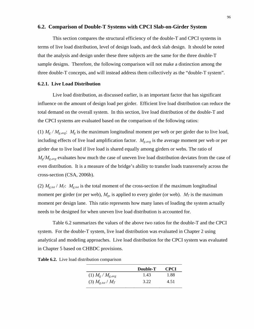
96

6.2. Comparison of Double-T Systems with CPCI Slab-on-Girder System

This section compares the structural efficiency of the double-T and CPCI systems in

terms of live load distribution, level of design loads, and deck slab design. It should be noted

that the analysis and design under these three subjects are the same for the three double-T

sample designs. Therefore, the following comparison will not make a distinction among the

three double-T concepts, and will instead address them collectively as the “double-T system”.

6.2.1. Live Load Distribution

Live load distribution, as discussed earlier, is an important factor that has significant

influence on the amount of design load per girder. Efficient live load distribution can reduce the

total demand on the overall system. In this section, live load distribution of the double-T and

the CPCI systems are evaluated based on the comparison of the following ratios:

(1) Mg / Mg,avg: Mg is the maximum longitudinal moment per web or per girder due to live load,

including effects of live load amplification factor. Mg,avg is the average moment per web or per

girder due to live load if live load is shared equally among girders or webs. The ratio of

Mg/Mg,avg evaluates how much the case of uneven live load distribution deviates from the case of

even distribution. It is a measure of the bridge’s ability to transfer loads transversely across the

cross-section (CSA, 2006b).

(2) Mg,tot / MT: Mg,tot is the total moment of the cross-section if the maximum longitudinal

moment per girder (or per web), Mg, is applied to every girder (or web). MT is the maximum

moment per design lane. This ratio represents how many lanes of loading the system actually

needs to be designed for when uneven live load distribution is accounted for.

Table 6.2 summarizes the values of the above two ratios for the double-T and the CPCI

system. For the double-T system, live load distribution was evaluated in Chapter 2 using

analytical and modeling approaches. Live load distribution for the CPCI system was evaluated

in Chapter 5 based on CHBDC provisions.

Table 6.2. Live load distribution comparison

Double-T CPCI (1) Mg / Mg,avg 1.43 1.88 (3) Mg,tot / MT 3.22 4.51

97

The ratios in Table 6.2 suggest that the double-T system is overall more efficient in live

load distribution. The comparison of the first ratio Mg/Mg,avg indicates that the maximum live

load per girder for the CPCI system deviates more from the ideal case of equal distribution. The

second ratio Mg,tot / MT clearly shows that the total live load demand on the full cross-section is

lower for the double-T system. The difference between the two systems is approximately 30%.

The inefficiency of live load distribution in the CPCI system comes from two levels. The first

level is the basic inefficiency associated with structural system itself. Due to flexibility of the

deck slab, live load only propagates to a few girders close to its point of application. This

uneven distribution is magnified by the relatively large number of girders in the system. The

second level of inefficiency is associated with the method of calculation. As discussed in

Chapter 5, live load distribution in a slab-on-girder system with multiple girders is a relatively

complex problem that involves many parameters. The provisions in codes and standards are

usually simplified representation of the real situation and include only a limited number of

variables. These provisions are usually used to determine the maximum amount of load

distributed to a girder under the most unfavourable conditions.

As the above comparison indicates, the double-T system exhibits more efficient live load

distribution. This has significant impact on the total live load demand on the structure. This

subject is examined in the following section.

6.2.2. Design Load

The structural efficiency of the double-T and the CPCI system can also be evaluated

from the perspective of design loads. Although the sample designs are developed under the

same geometrical conditions and live load model, the amount of dead and live load incurred in

each structure are different. The difference in dead load is due to the structures’ different cross-

sections, while the difference in live load results from the variation in live load distribution.

The maximum moment intensities for the double-T and the CPCI systems are

summarized in Table 6.3. To present a more clear comparison, the moment intensity ratios of

the two systems are computed for each load category as well as for the overall structure. The

values from Table 6.3 clearly indicate that the double-T system incurs less design load. While

the amount of super-imposed dead load is the same for both systems, the dead load moment

intensity in the double-T is only 69% of that in the CPCI system. This is largely due to the

small number of webs in the double-T cross-section as well as the web’s slender dimension.

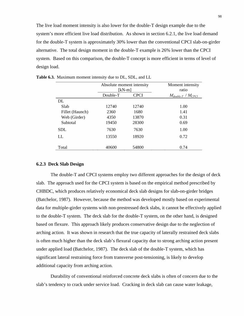
98

The live load moment intensity is also lower for the double-T design example due to the

system’s more efficient live load distribution. As shown in section 6.2.1, the live load demand

for the double-T system is approximately 30% lower than the conventional CPCI slab-on-girder

alternative. The total design moment in the double-T example is 26% lower than the CPCI

system. Based on this comparison, the double-T concept is more efficient in terms of level of

design load.

Table 6.3. Maximum moment intensity due to DL, SDL, and LL

Absolute moment intensity [kN-m] Moment intensity

ratio Double-T CPCI Mdouble-T / MCPCI DL Slab 12740 12740 1.00 Fillet (Haunch) 2360 1680 1.41 Web (Girder) 4350 13870 0.31 Subtotal 19450 28300 0.69

SDL 7630 7630 1.00

LL 13550 18920 0.72 Total 40600 54800 0.74

6.2.3 Deck Slab Design

The double-T and CPCI systems employ two different approaches for the design of deck

slab. The approach used for the CPCI system is based on the empirical method prescribed by

CHBDC, which produces relatively economical deck slab designs for slab-on-girder bridges

(Batchelor, 1987). However, because the method was developed mostly based on experimental

data for multiple-girder systems with non-prestressed deck slabs, it cannot be effectively applied

to the double-T system. The deck slab for the double-T system, on the other hand, is designed

based on flexure. This approach likely produces conservative design due to the neglection of

arching action. It was shown in research that the true capacity of laterally restrained deck slabs

is often much higher than the deck slab’s flexural capacity due to strong arching action present

under applied load (Batchelor, 1987). The deck slab of the double-T system, which has

significant lateral restraining force from transverse post-tensioning, is likely to develop

additional capacity from arching action.

Durability of conventional reinforced concrete deck slabs is often of concern due to the

slab’s tendency to crack under service load. Cracking in deck slab can cause water leakage,

99

which is a vector in reinforcement corrosion. In comparison, the deck slab of the double-T

system has superior durability. By pre-compressing the concrete, transverse post-tensioning

reduces the likelihood for cracks to develop, thus enhances the deck slab’s intrinsic durability.

6.3. Material Consumption

6.3.1. Concrete

Concrete consumption in the double-T and the CPCI system is summarized in Table 6.4.

The table includes data on concrete volume used in the full system as well as in each structural

component. Structural components are categorized into “primary section”, such as the double-T

girder in the double-T system and the slab-girder composite in the CPCI system, and

“diaphragms”.

Table 6.4. Concrete consumption

Concrete volume [m3] % of total volume Double-T* CPCI Double-T* CPCI

Primary section Deck slab 114 114 50% 39% Fillet (Haunch) 21 15 9% 5% Web (Girder) 39 124 17% 43%

Subtotal 174 252 77% 88%

Diaphragms End diaphragm 36 36 16% 13% Deviation diaphragm 15 0 7% 0%

Subtotal 52 36 23% 13%

Grand total 225 288 100% 100%

* Because the three double-T sample designs share the same concrete section, they are collectively represented here as “Double-T”.

As shown in the above table, the total concrete consumption of the double-T system is

approximately 22% less than the CPCI system. The material economy of the double-T system

can be attributed to its efficient cross-section which consists of only two slender webs. The

amount of concrete consumed by the double-T webs is only 1/3 of the amount consumed by the

CPCI girders. The concrete consumption in end diaphragms has no major discrepancy between

the two systems. The deviation diaphragm, which is only required in the double-T concept,

consumes approximately 7% of total concrete used in the double-T system.

100

Another important trend shown in Table 6.4 is that deck slabs tend to be the most major

source of concrete consumption in bridge systems. For the sample design of the conventional

CPCI slab-on-girder bridge, deck slab takes up 39% of total superstructure concrete. For the

more slender double-T girder bridge, the deck slab’s share increases to 50% of the system’s total

concrete consumption. This observation suggests that deck slab design is an important subject

that has significant impact on the structure’s overall material economy. For instance, if the deck

slab thickness can be reduced by 25 mm, the total concrete consumption in the double-T sample

design can be reduced by close to 6%. The deck slab for the double-T system is designed based

on flexure. As discussed earlier in this chapter, this method tends to be conservative as deck

slabs usually exhibit greater capacity than their flexural strength due to arching action.

However, empirical method prescribed by CHBDC is not fully applicable to the double-T

system because the method is mostly based on research data of multiple-girder systems. To

further improve the material economy of the double-T system and other bridge systems, deck

slab design is a subject that deserves further investigation.

6.3.2. Prestressing Steel

Prestressing steel consumption is summarized in Table 6.5. All three double-T systems

use less prestressing steel in longitudinal post-tensioning than the CPCI system. However, the

double-T systems require additional prestressing steel in the transverse post-tensioning of deck

slabs. As a result, the total volume of prestressing steel consumed by the double-T systems

becomes close to or higher than the CPCI system. Despite the cost, transverse post-tensioning

brings additional value to the system by improving the deck slab’s durability and enhancing the

structure’s overall quality.

Table 6.5. Prestressing steel consumption [unit: t]

Double-T

base conceptDouble-T

alternative I Double-T

alternative II CPCI Longitudinal post-tensioning 6.3 5.9 5.9 8.6 Transverse post-tensioning 2.7 2.7 2.7 - Unstressed prestressing steel - - 0.7 -

Total 9.0 8.5 9.3 8.6

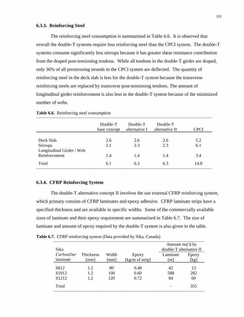
101

6.3.3. Reinforcing Steel

The reinforcing steel consumption is summarized in Table 6.6. It is observed that

overall the double-T systems require less reinforcing steel than the CPCI system. The double-T

systems consume significantly less stirrups because it has greater shear resistance contribution

from the draped post-tensioning tendons. While all tendons in the double-T girder are draped,

only 36% of all prestressing strands in the CPCI system are deflected. The quantity of

reinforcing steel in the deck slab is less for the double-T system because the transverse

reinforcing steels are replaced by transverse post-tensioning tendons. The amount of

longitudinal girder reinforcement is also less in the double-T system because of the minimized

number of webs.

Table 6.6. Reinforcing steel consumption

Double-T

base conceptDouble-T


alternative II CPCI Deck Slab 2.6 2.6 2.6 5.2 Stirrups 2.1 2.3 2.3 6.1 Longitudinal Girder / Web Reinforcement 1.4 1.4 1.4 3.4

Total 6.1 6.3 6.3 14.8

6.3.4. CFRP Reinforcing System

The double-T alternative concept II involves the use external CFRP reinforcing system,

which primary consists of CFRP laminates and epoxy adhesive. CFRP laminate strips have a

specified thickness and are available in specific widths. Some of the commercially available

sizes of laminate and their epoxy requirement are summarized in Table 6.7. The size of

laminate and amount of epoxy required by the double-T system is also given in the table.

Table 6.7. CFRP reinforcing system (Data provided by Sika, Canada)

Amount req’d by

double-T alternative IIThickness Width Epoxy Laminate Epoxy

Sika CarbonDur laminate [mm] [mm] [kg/m of strip] [m] [kg]

S812 1.2 80 0.48 42 13 S1012 1.2 100 0.60 588 282 S1212 1.2 120 0.72 84 60

Total - 355

102

6.4. Cost Comparison

6.4.1. Cost Comparison of Double-T Systems

The cost of the three double-T systems will be compared in this section. The cost of

precast concrete, including fabrication, delivery and erection, is the same for the three systems.

The cost of structural reinforcements, such as post-tensioning, CFRP, and unstressed

prestressing steel, are compared based on the material unit costs listed in Table 6.8, which are

acquired from design offices and suppliers. The unit cost of post-tensioning already accounts

for the cost of anchorage systems and the labour required for stressing the tendons.

Table 6.8. Unit cost of structural reinforcing systems

Unit cost Post-tensioning Longitudinal [$/t] 8,500 Transverse [$/t] 11,500 CFRP system CFRP laminate [avg $/m] 58 Epoxy [$/kg] 14 Unstressed strand [$/t] 2,500

The cost estimate for the three systems based on the above material unit cost is

summarized in Table 6.9. The cost of precast concrete is assumed to be a constant value of C

for the three systems. The comparison indicates that double-T alternative II is the most

economical system. The cost of alternative concept I is relatively high due to the high cost of

CFRP reinforcing system.

Table 6.9. Cost comparison of double-T systems [Unit: $]

Double-T base

concept Double-T


alternative II

Precast concrete C C C Post-tensioning Longitudinal 53,918 49,770 49,770 Transverse 30,970 30,970 30,970 CFRP system CFRP 43,680 Epoxy 5,093 Unstressed strand 1,826

Total C + 84,900 C + 129,500 C + 81,800

103

6.4.2. Cost Comparison between Double-T and CPCI Systems

In this section, the cost of the CPCI slab-on-girder system is compared with double-T

system. The cost of the CPCI system primarily consists of precast concrete and cast-in-place

deck slab. For the double-T system, the cost primarily consists of precast concrete and

structural reinforcing systems.

The cost of precast concrete is the most uncertain item in this cost comparison. It is not

only affected by the cost of material and labour, but also the availability of suppliers in the

market. The cost associated with the fabrication, delivery and erection of the precast concrete is

summarized in Table 6.10 and discussed in the following paragraphs:

Precast concrete fabrication:

The fabrication cost depends on the actual material cost as well as the ease of fabrication

and the availability of suppliers. In terms of materials, the double-T system requires only

concrete and reinforcing bars while the CPCI system requires additional prestressing strands for

pre-tensioning. However, the cost of concrete in the double-T system is likely higher because it

utilizes a higher strength concrete. In terms of forming, the double-T system can be casted

relatively easily with wood formworks. Because the relative ease of forming and low cost of the

forms, supplier availability is likely not a problem, and the contractor may be able to form the

segments themselves. On the other hand, the CPCI girders need specialized formworks and

equipments that require high capital investment. This results in a very limited number of

suppliers available. In Ontario where there are only several CPCI girder suppliers, the price of

CPCI girders can increase due to the combination of low supply and high demand. Based on the

above comparison, it is expected that the precast concrete fabrication cost would be similar

between the double-T and the CPCI system.

Precast concrete delivery:

The CPCI girders usually come in lengths of about 30, 35 or 40 m. The long segments

require special trucks, permits and specified routes. On the other hand, the smaller double-T

segments can be transported without special consideration. Hence, it is expected that the

delivery cost is lower for the double-T system.

Erection:

The erection of CPCI girders requires a crane while the double-T system requires a crane

and an erection girder. The crane needed by the double-T system can be smaller than the CPCI

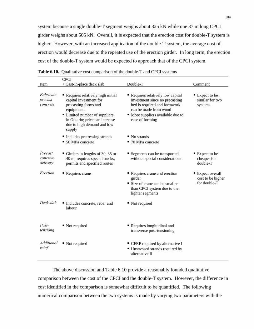
104

system because a single double-T segment weighs about 325 kN while one 37 m long CPCI

girder weighs about 505 kN. Overall, it is expected that the erection cost for double-T system is

higher. However, with an increased application of the double-T system, the average cost of

erection would decrease due to the repeated use of the erection girder. In long term, the erection

cost of the double-T system would be expected to approach that of the CPCI system.

Table 6.10. Qualitative cost comparison of the double-T and CPCI systems

Item CPCI + Cast-in-place deck slab Double-T Comment

Fabricate precast concrete

Requires relatively high initial capital investment for precasting forms and equipments

Limited number of suppliers in Ontario; price can increase due to high demand and low supply

Requires relatively low capital investment since no precasting bed is required and formwork can be made from wood

More suppliers available due to ease of forming

Expect to be similar for two systems

Includes pretressing strands No strands 50 MPa concrete 70 MPa concrete

Precast concrete delivery

Girders in lengths of 30, 35 or 40 m; requires special trucks, permits and specified routes

Segments can be transported without special considerations

Expect to be cheaper for double-T

Erection Requires crane

Requires crane and erection girder

Size of crane can be smaller than CPCI system due to the lighter segments

Expect overall cost to be higher for double-T

Deck slab Includes concrete, rebar and

labour

Not required

Post-tensiong

Not required Requires longitudinal and transverse post-tensioning

Additional reinf.

Not required CFRP required by alternative I Unstressed strands required by alternative II

The above discussion and Table 6.10 provide a reasonably founded qualitative

comparison between the cost of the CPCI and the double-T system. However, the difference in

cost identified in the comparison is somewhat difficult to be quantified. The following

numerical comparison between the two systems is made by varying two parameters with the

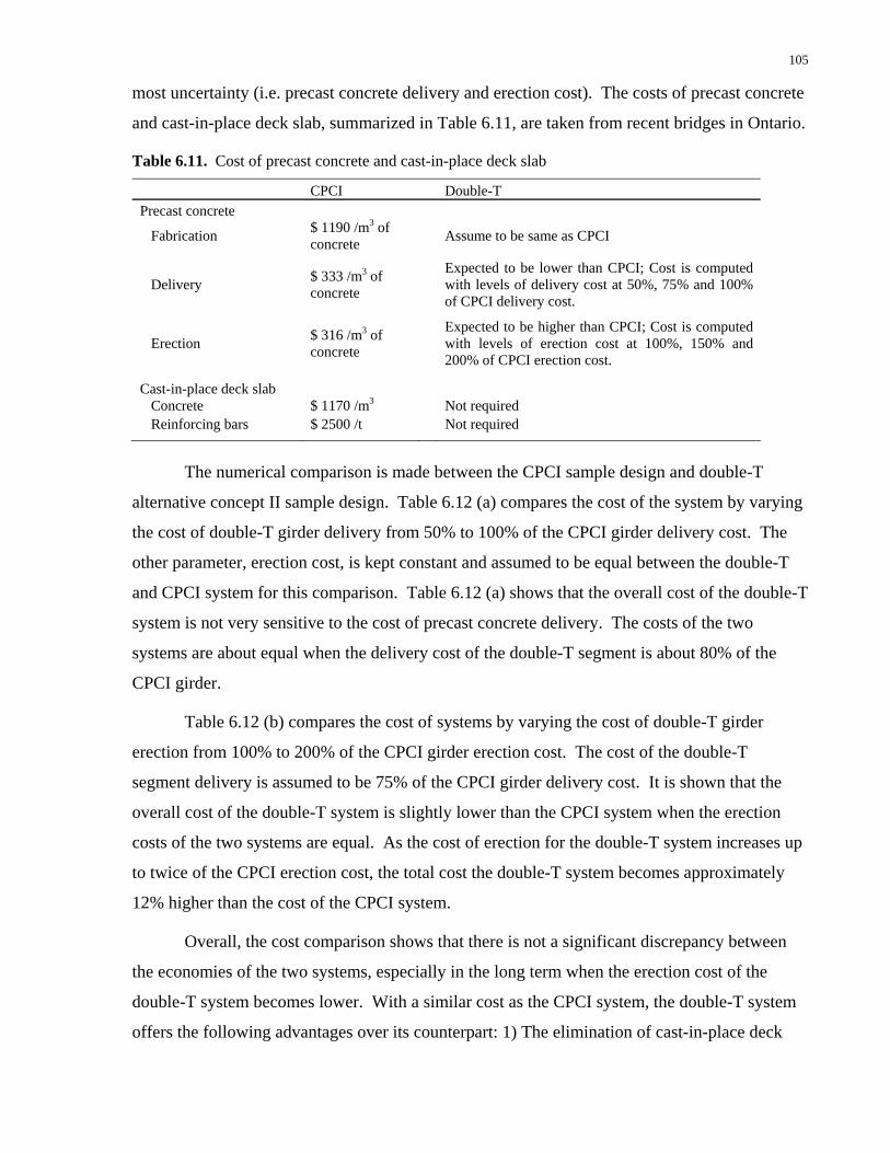
105

most uncertainty (i.e. precast concrete delivery and erection cost). The costs of precast concrete

and cast-in-place deck slab, summarized in Table 6.11, are taken from recent bridges in Ontario.

Table 6.11. Cost of precast concrete and cast-in-place deck slab

CPCI Double-T Precast concrete

Fabrication $ 1190 /m3 of concrete Assume to be same as CPCI

Delivery $ 333 /m3 of concrete

Expected to be lower than CPCI; Cost is computed with levels of delivery cost at 50%, 75% and 100% of CPCI delivery cost.

Erection $ 316 /m3 of concrete

Expected to be higher than CPCI; Cost is computed with levels of erection cost at 100%, 150% and 200% of CPCI erection cost.

Cast-in-place deck slab Concrete $ 1170 /m3 Not required Reinforcing bars $ 2500 /t Not required

The numerical comparison is made between the CPCI sample design and double-T

alternative concept II sample design. Table 6.12 (a) compares the cost of the system by varying

the cost of double-T girder delivery from 50% to 100% of the CPCI girder delivery cost. The

other parameter, erection cost, is kept constant and assumed to be equal between the double-T

and CPCI system for this comparison. Table 6.12 (a) shows that the overall cost of the double-T

system is not very sensitive to the cost of precast concrete delivery. The costs of the two

systems are about equal when the delivery cost of the double-T segment is about 80% of the

CPCI girder.

Table 6.12 (b) compares the cost of systems by varying the cost of double-T girder

erection from 100% to 200% of the CPCI girder erection cost. The cost of the double-T

segment delivery is assumed to be 75% of the CPCI girder delivery cost. It is shown that the

overall cost of the double-T system is slightly lower than the CPCI system when the erection

costs of the two systems are equal. As the cost of erection for the double-T system increases up

to twice of the CPCI erection cost, the total cost the double-T system becomes approximately

12% higher than the cost of the CPCI system.

Overall, the cost comparison shows that there is not a significant discrepancy between

the economies of the two systems, especially in the long term when the erection cost of the

double-T system becomes lower. With a similar cost as the CPCI system, the double-T system

offers the following advantages over its counterpart: 1) The elimination of cast-in-place deck

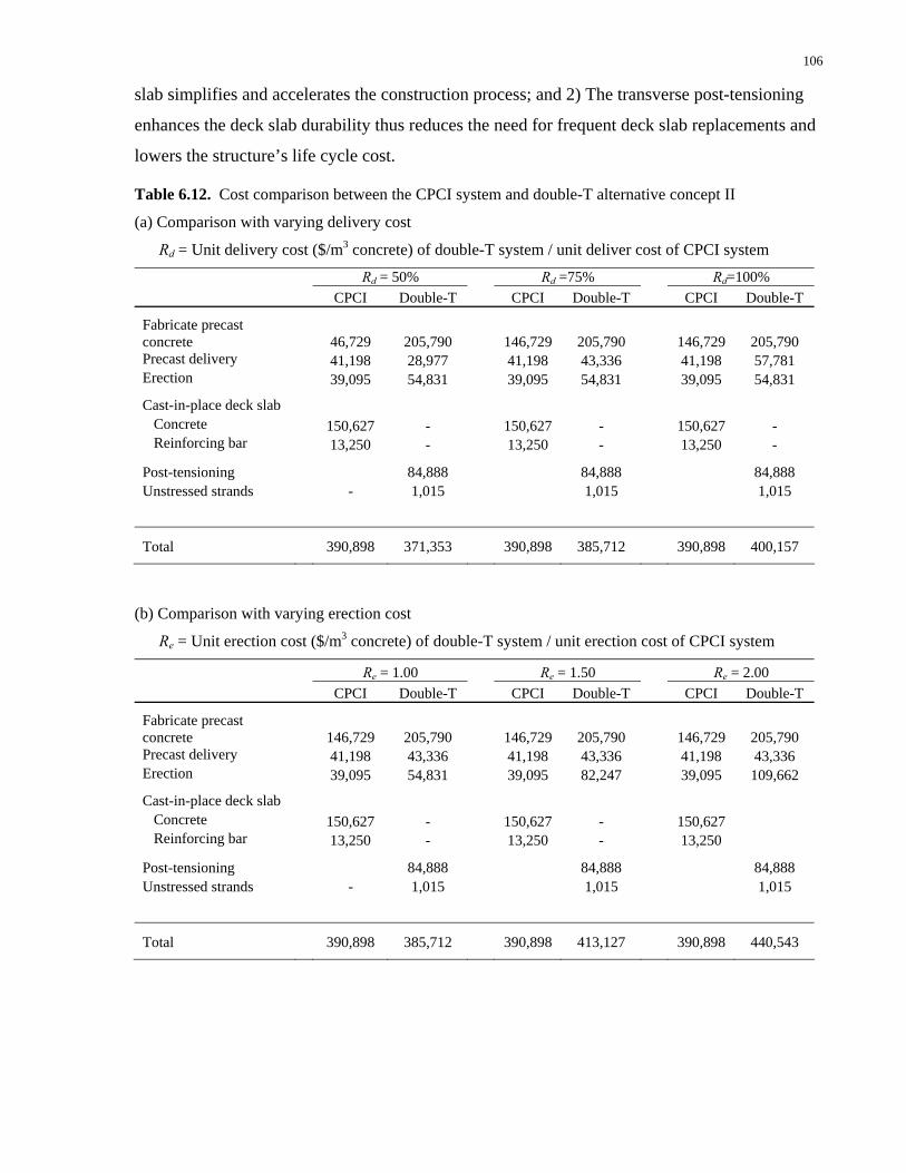
106

slab simplifies and accelerates the construction process; and 2) The transverse post-tensioning

enhances the deck slab durability thus reduces the need for frequent deck slab replacements and

lowers the structure’s life cycle cost.

Table 6.12. Cost comparison between the CPCI system and double-T alternative concept II

(a) Comparison with varying delivery cost

Rd = Unit delivery cost ($/m3 concrete) of double-T system / unit deliver cost of CPCI system

Rd = 50% Rd =75% Rd=100% CPCI Double-T CPCI Double-T CPCI Double-T

Fabricate precast concrete 46,729 205,790 146,729 205,790 146,729 205,790 Precast delivery 41,198 28,977 41,198 43,336 41,198 57,781 Erection 39,095 54,831 39,095 54,831 39,095 54,831

Cast-in-place deck slab Concrete 150,627 - 150,627 - 150,627 - Reinforcing bar 13,250 - 13,250 - 13,250 -

Post-tensioning 84,888 84,888 84,888 Unstressed strands - 1,015 1,015 1,015

Total 390,898 371,353 390,898 385,712 390,898 400,157

(b) Comparison with varying erection cost

Re = Unit erection cost ($/m3 concrete) of double-T system / unit erection cost of CPCI system

Re = 1.00 Re = 1.50 Re = 2.00 CPCI Double-T CPCI Double-T CPCI Double-T

Fabricate precast concrete 146,729 205,790 146,729 205,790 146,729 205,790 Precast delivery 41,198 43,336 41,198 43,336 41,198 43,336 Erection 39,095 54,831 39,095 82,247 39,095 109,662

Cast-in-place deck slab Concrete 150,627 - 150,627 - 150,627 Reinforcing bar 13,250 - 13,250 - 13,250

Post-tensioning 84,888 84,888 84,888 Unstressed strands - 1,015 1,015 1,015

Total 390,898 385,712 390,898 413,127 390,898 440,543

Chapter 7 Conclusion

This thesis develops three alternative double-T bridge concepts and compares their

primary superstructure material consumption with that of a conventional single span CPCI

system. The results indicate that the double-T systems are in general more efficient than the

CPCI system and have the potential to achieve better material economy.

Three double-T concepts are developed with varying design of primary longitudinal

reinforcements. All three concepts employ a slender concrete cross-section with two thin webs,

post-tensioning in two orthogonal directions, and precast segmental construction method. The

double-T base concept developed in Chapter 2 is reinforced with pure external unbonded post-

tensioning. While a feasible sample design is created based on the given geometrical

requirements, the concept is found to have a somewhat low tolerance in terms of post-tensioning

design due to the high jacking force imposed to the system during construction. To resolve this

limitation and extend the double-T concept’s applicability to a wider range of geometrical

conditions, two alternative double-T concepts with blends of prestressed and non-prestressed

primary reinforcements are developed in Chapter 3 and 4. They are modifications of the base

concept with reduced amounts of post-tensioning and supplementary non-prestressed

reinforcements. These modifications in the system create more flexibility in the design because:

1) The decrease in post-tensioning reduces the negative moment imposed on the structure during

construction thus making the structure less critical in negative flexure; 2) The addition of the

non-prestressed continuous reinforcements expands the allowable window for concrete stress

from 0.6 f’c – 0 to 0.6 f’c – fcr under SLS. The alternative concept I with CFRP reinforcing

system is limited by the CFRP debonding strain under ULS. The alternative concept II does not

have such a limitation. As a result, it achieves slightly larger deformation and develops higher

stress in the unbonded tendons under ULS, which are indicative of a more efficient utilization of

the unbonded tendons.

107

108

Comparisons of the double-T and CPCI systems are presented in Chapter 6. The

structural efficiency comparison indicates that the double-T section with two slender webs not

only reduces the overall concrete and dead load of the structure, but also improves live load

distribution in comparison with conventional CPCI system. The use of transverse post-

tensioning in the double-T deck slab enhances the system’s durability. The costs of the double-

T and the CPCI systems are compared both qualitatively and quantitatively. It is found that

there is not a significant discrepancy between the economies of the two systems, especially in

the long term when the erection cost of the double-T system becomes lower. With a similar cost

as the CPCI system, the double-T system offers advantages over its counterpart, such as

simplified construction process and enhanced deck slab durability.

References

American Association of State Highway and Transportation Officials (AASHTO). (1996).

Standard specifications for highway bridges. Washington, D.C.

American Association of State Highway and Transportation Officials (AASHTO). (1998).

LRFD bridge design specifications. (SI units 2nd ed.). Washington, D.C.

American Composites Manufacturers Association (ACMA). (2005). Composites Industry

Statistics. <http://www.acmanet.org/professionals /2005-Composites-Industry-

Statistics.pdf > (Nov. 20, 2009)

American Concrete Institute (ACI) – Committee 440. (2007). Report on Fiber-Reinforced

Polymer (FRP) Reinforcement for Concrete Structures, ACI 440R-07. Farmington Hills,

MI, USA.

American Concrete Institute (ACI) – Committee 440. (2008). Design and Construction of

Externally Bonded FRP Systems, ACI 440.2R-08. Farmington Hills, MI, USA.

American Segmental Bridge Institute (2008). Segmental Box Girder Standards.

<http://www.asbi-assoc.org/resources/AASHTO_Standards.cfm> (June 1, 2008)

Batchelor, B. deV. (1987). Membrane Enhancement in Top Slabs of Concrete Bridges. Chapter

6 of Concrete Bridge Engineering: Performance and Advances. Elsevier Applied

Science Publishers Ltd., Barking, Essex, England.

Cai, C. S. (2005). Discussion on AASHTO LRFD load distribution factors for slab-on-girder

bridges. Practice Periodical on Structural Design and Construction, 10(3), 171-176.

Canadian Precast/Prestressed Concrete Instittute (2009). Prestressed Girder Bridges.

<http://www.cpci.ca/?sc=bs&pn=prestressedgirderbridges> (August 1, 2009)

109

110

Canadian Standards Association (2002). S806-02: Design and Construction of Building

Components with Fibre-Reinforced Polyers. CSA, Mississauga, Ontario.

Canadian Standards Association (2006a). CAN/CSA-S6-06: Canadian Highway Bridge Design

Code. CSA, Mississauga, Ontario.

Canadian Standards Association (2006b). S6.1-06: Commentary on CAN/CSA-S6-06, Canadian

Highway Bridge Design Code. CSA, Mississauga, Ontario.

Choi, W., Rizkalla, S., Zia, P., & Mirmiran, A. (2008). Behavior and design of high-strength

prestressed concrete girders. PCI Journal, 53(5), 54-69.

Departement des Travaux Publics du Canton de Vaud. (1989). Catalogue of le viaduc d’Orbe for

Routes nationales suisses N9.

Dywidag-Systems International Canada Ltd. (2006). DYWIDAG Multistrand Stay Cable

Systems. <http://www.dsicanada.ca/en/downloads/brochures-canada.html> (April 1,

2008).

Dunker, K. F. (1992). Performance of Prestressed Concrete Highway Bridges in the United

States – The First 40 Years. PCI Journal, 37(3), 48-64.

Federal Highway Administration (FHWA). (2009). Optimized Sections for High-Strength

Concrete Bridge Girders--Effect of Deck Concrete Strength.

<http://www.tfhrc.gov/structur/pubs/05058/01.htm> (Oct. 10, 2009)

Gauvreau, P. (2006). Bridges. Chapter 12 (pp. 195-240) of Post-Tensioning Manual. 6th ed.

Phoenix: Post-Tensioning Institute.

Hassanain. M. A. (1998). Optimal design of precast I-girder bridges made with high-

performance concrete. Unpublished Doctor of Philosophy, Department of Civil

Engineering, Calgary, Alberta.

Hewitt, B. E., & Batchelor, B. d. (1975). Punching shear strength of restrained slabs. ASCE J

Struct Div, 101(9), 1837-1853.

111

Interactive Design Systems. (2009). <http://www.ids-

soft.com/solutions/products/geometrey.html Match cast diagram> (Nov. 11, 2009)

Kulka, F., & Lin, T. Y. (1982). Comparative studies of medium span box girder bridges with

other precast systems. International Conference on Short and Medium Span Bridges,

Proceedings, 1 81-94.

Leonhardt, Fritz. (1979). Vorlesungen uber Massivbau. Berlin: Springer-Verlag.

Lounis, Z., Mirza, M. S., & Cohn, M. Z. (1997). Segmental and conventional precast prestressed

concrete I-bridge girders. Journal of Bridge Engineering, 2(3), 73-82.

Menn, C. (1990). In Gauvreau P. (Ed.), Prestressed concrete bridges. Boston: Birkhäuser

Verlag.

MTO. (2002). Prestressed Girders and Bearings (CPCI 1900). Standard Drawing June 2002.

Pre-Con. (2004). Prestressed “I” Girders. Product Manual.

Pucher, A. (1977). Einflussfelder elastischer platten: Influence surfaces of elastic plates (5.,

durchgesehene Aufl. -- ed.). New York: Springer-Verlag.

Roberts-Wollmann, C. L., Kreger, M. E., Rogowsky, D. M., & Breen, J. E. (2005). Stresses in

external tendons at ultimate. ACI Structural Journal, 102(2), 206-213.

Schlaich, J., Shäfer, K., and Jennewein, M. (1987). Towards a Consistent Design of Structural

Concrete. PCI Journal. 32, 3: 74-150.

Sika. (2009). Engineering with external carbon reinforcement. <http://www.sika.ca/con-bro-

carbon-reinforcement-heinz.pdf> (Nov. 3, 2009)

Sika. (2009). Sika CarboDur product data sheet. <http://www.sika.ca/con-tds-sikacarbodur-

ca.pdf> (Nov. 3, 2009)

Stussi, B., (1958). Grundsatzliches zum Projekt, zur Ausfuhrung und zur Berechnung. In

Offentlichen Bauten des Kantons, Weinlandbrucke Andelfingen (32-47).

112

Suksawang, N., & Nassif, H. H. (2007). Development of live load distribution factor equation

for girder bridges. Transportation Research Record, no.2028, (2028), 9-18.

Teng, J. (2002). FRP Strengthened RC Structures. New York: Wiley.

Trost, H. (1967). Auswirkungen des Superpositionsprinzips auf Kriech- und

Relaxationsprobleme bei Beton und Spannbeton. Parts 1, 2. Beton- und Stahlbetonbau.

Washington State Department of Transportation. (2008). Single Span P.S Girder Construction

Sequence. Bridge Standard Drawings.

<http://www.wsdot.wa.gov/eesc/bridge/drawings/index.cfm?fuseaction=drawings&secti

on_nbr=6&type_id=16> (August 1, 2009)

Yousif, Z., & Hindi, R. (2007). AASHTO-LRFD live load distribution for beam-and-slab

bridges: Limitations and applicability. Journal of Bridge Engineering, 12(6), 765-773.

Appendix A:

Double-T Concepts Sample Calculations and Design Drawings

113

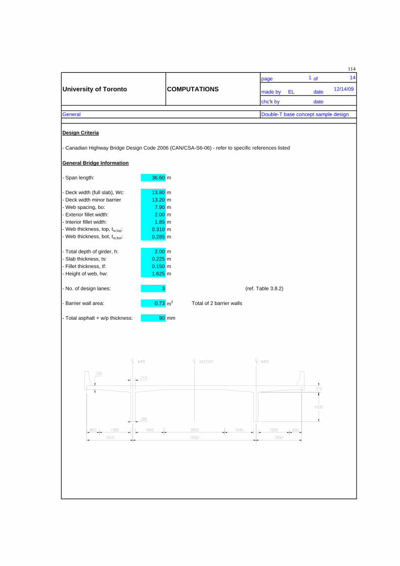
114

page 1 of 14

University of Toronto COMPUTATIONS made by EL date 12/14/09

chc'k by date

General Double-T base concept sample design

Design Criteria

- Canadian Highway Bridge Design Code 2006 (CAN/CSA-S6-06) - refer to specific references listed

General Bridge Information

- Span length: 36.60 m

- Deck width (full slab), Wc: 13.80 m- Deck width minor barrier 13.20 m- Web spacing, bo: 7.90 m- Exterior fillet width: 2.00 m- Interior fillet width: 1.85 m- Web thickness, top, tw,top: 0.310 m- Web thickness, bot, tw,bot: 0.285 m

- Total depth of girder, h: 2.00 m- Slab thickness, ts: 0.225 m- Fillet thickness, tf: 0.150 m- Height of web, hw: 1.625 m

- No. of design lanes: 3 (ref. Table 3.8.2)

- Barrier wall area: 0.73 m2 Total of 2 barrier walls

- Total asphalt + w/p thickness: 90 mm

115

page 2 of 14


chc'k by date

Section Property Double-T base concept sample design

Section Properties - Full section

Atot = 4.741 m2Ytop = 0.353 m Ybot = 1.647 m

I = 1.065 m4Stop = 3.019 m3 Sbot = 0.647 m3

Section Property - Half sectionAtot = 2.370 m2Ytop = 0.353 m Ybot = 1.647 m

I = 0.533 m4Stop = 1.509 m3 Sbot = 0.323 m3

116

page 3 of 14


chc'k by date

Material Property Double-T base concept sample design

Material Specifications

Post-tensioning tendon and duct Use DSI 27-0.6" strand ducts

Strand diameter = 13.35 mm2

Strand area = 140 mm2

No. of strands per duct = 27

f pu = 1860 MPa Assume fpy = 0.9 fpu = 1674 MPaEp = 200000 MPa (cl. 8.4.3.3)

Concrete Ec= (3000 (fC')0.5 + 6900) (gC / 2300)1.5 (cl. 8.4.1.7)b1 = 0.97 - 0.0025 fC' > 0.67 (cl. 8.8.3.g)

f'c (Girder) = 70 MPa ===> Ec= 36263 MPa b1 = 0.795 fCR = 3.35

Reinforcing Steelfy = 400 MPa

Es = 200000 MPa (cl. 8.4.2.1.4)

117

page 4 of 14


chc'k by date

Torsion 1 Double-T Concrete Bridge Design

Torsion in Double-T Girders(Ref. Menn, Sec. 5.1.3) - Torsional moments in open sections (i.e. double-t girder) are resisted by a combnation of St. Venant torsion (Tsv) and warping torsion (Tw).

Calculate k

ho = 1.8632609 mbo = 7.90 m

h = 2.00 mb = 13.80 m

bw = 0.2975 mts = 0.2734783 m

as: distance from middle surface of top slab to centroidal axisas = 0.216102 m I (half) = 0.53254 m4

an: distance from middle surface of top slab to neutral axis.an = 0.208767 m In bar (half) = 0.59369 m4

K: torsional constant (equivalent of I in bending)K = 0.126793 G = 0.4 E

Compatibility at mid-spanspan = 36.60 m

sv = 9.15 k*Qw*bo/(G*K) = 1425.25 k*(Qw/E) [m-2]

wv: delfection at mid-spanwv = Qw*l^3/(48*E*I n bar) = 1720.47 Qw/E [m-1]

w = 2*wv(x)/bo = 435.561 Qw/E [m-2]

Set w = sv

k = 0.305603Qw = 0.76593 Q and Qsv = 0.23407 Q

)()()( xTxTxT wsv kxTxT

w

sv

)()( k

QQ

w

sv

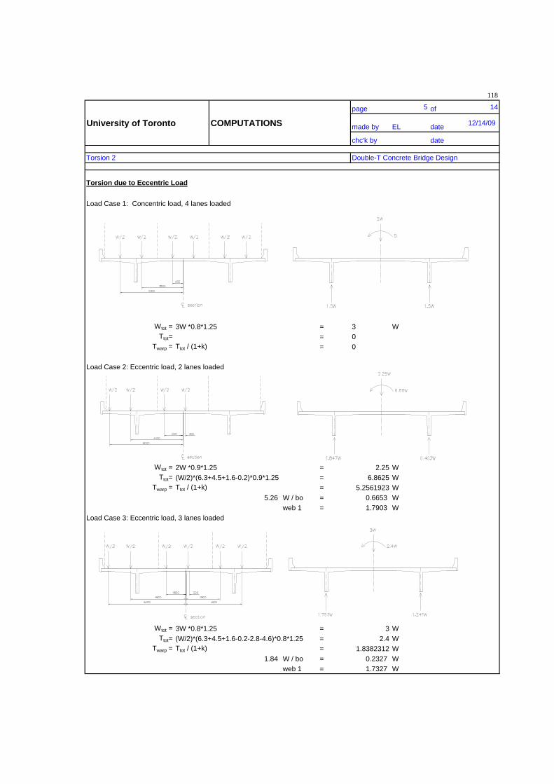
118

page 5 of 14


chc'k by date

Torsion 2 Double-T Concrete Bridge Design

Torsion due to Eccentric Load

Load Case 1: Concentric load, 4 lanes loaded

Wtot = 3W *0.8*1.25 = 3 WTtot= = 0

Twarp = Ttot / (1+k) = 0

Load Case 2: Eccentric load, 2 lanes loaded

Wtot = 2W *0.9*1.25 = 2.25 WTtot= (W/2)*(6.3+4.5+1.6-0.2)*0.9*1.25 = 6.8625 W

Twarp = Ttot / (1+k) = 5.2561923 W5.26 W / bo = 0.6653 W

web 1 = 1.7903 WLoad Case 3: Eccentric load, 3 lanes loaded

Wtot = 3W *0.8*1.25 = 3 WTtot= (W/2)*(6.3+4.5+1.6-0.2-2.8-4.6)*0.8*1.25 = 2.4 W

Twarp = Ttot / (1+k) = 1.8382312 W1.84 W / bo = 0.2327 W

web 1 = 1.7327 W

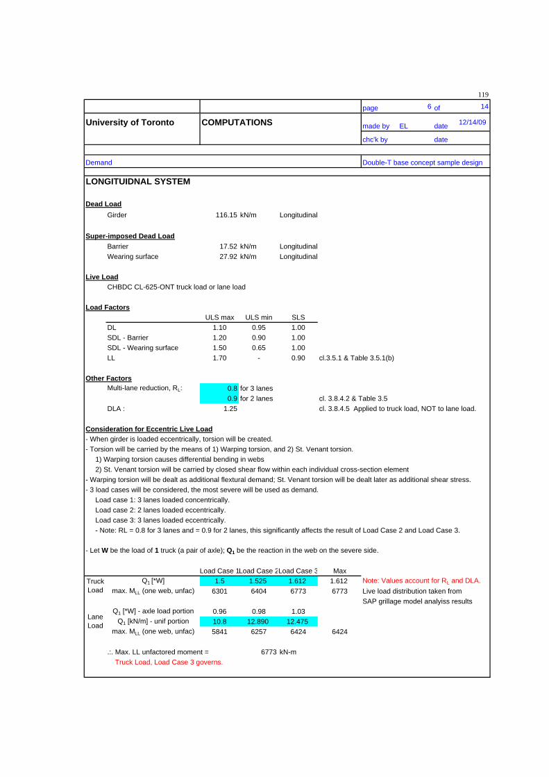
119

page 6 of 14


chc'k by date

Demand Double-T base concept sample design

LONGITUIDNAL SYSTEM

Dead LoadGirder 116.15 kN/m Longitudinal

Super-imposed Dead LoadBarrier 17.52 kN/m LongitudinalWearing surface 27.92 kN/m Longitudinal

Live LoadCHBDC CL-625-ONT truck load or lane load

Load FactorsULS max ULS min SLS

DL 1.10 0.95 1.00SDL - Barrier 1.20 0.90 1.00SDL - Wearing surface 1.50 0.65 1.00LL 1.70 - 0.90 cl.3.5.1 & Table 3.5.1(b)

Other FactorsMulti-lane reduction, RL: 0.8 for 3 lanes

0.9 for 2 lanes cl. 3.8.4.2 & Table 3.5DLA : 1.25 cl. 3.8.4.5 Applied to truck load, NOT to lane load.

Consideration for Eccentric Live Load- When girder is loaded eccentrically, torsion will be created.- Torsion will be carried by the means of 1) Warping torsion, and 2) St. Venant torsion. 1) Warping torsion causes differential bending in webs 2) St. Venant torsion will be carried by closed shear flow within each individual cross-section element- Warping torsion will be dealt as additional flextural demand; St. Venant torsion will be dealt later as additional shear stress.- 3 load cases will be considered, the most severe will be used as demand. Load case 1: 3 lanes loaded concentrically. Load case 2: 2 lanes loaded eccentrically. Load case 3: 3 lanes loaded eccentrically. - Note: RL = 0.8 for 3 lanes and = 0.9 for 2 lanes, this significantly affects the result of Load Case 2 and Load Case 3.

- Let W be the load of 1 truck (a pair of axle); Q1 be the reaction in the web on the severe side.

Load Case 1Load Case 2Load Case 3 MaxQ1 [*W] 1.5 1.525 1.612 1.612 Note: Values account for RL and DLA.

max. MLL (one web, unfac) 6301 6404 6773 6773 Live load distribution taken fromSAP grillage model analyiss results

Q1 [*W] - axle load portion 0.96 0.98 1.03Q1 [kN/m] - unif portion 10.8 12.890 12.475

max. MLL (one web, unfac) 5841 6257 6424 6424

.:. Max. LL unfactored moment = 6773 kN-m Truck Load, Load Case 3 governs.

LaneLoad

TruckLoad

120

page 7 of 14


chc'k by date

Load Combinations Double-T base concept sample design

Section Property - Full sectionAtot = 4.741 m2Ytop = 0.353 m Ybot = 1.647 m

I = 1.065 m4Stop = 3.019 m3 Sbot = 0.647 m3

Section Property - Half sectionAtot = 2.370 m2Ytop = 0.353 m Ybot = 1.647 m

I = 0.533 m4Stop = 1.509 m3 Sbot = 0.323 m3

Moments (ONE web)

DL SDL-Barrier SDL-WS LLMid-span 9724 1467 2337 6773Deviation 8286 1250 1992 6042 Deviation = 11.3 m from support

Anchorage 5950 898 1430 4361 6.9m from support

**Note: LL moment accounts for warping torsion.

Size of PT (ONE web)str./ duct no. duct Tot. str

Stage 1 27 2.00 54.00Stage 2 24 1.00 24.00

Total 78.00

Allowable stresses for SLSten fct = 0 Mpacomp f'c = 0.60 f'c = 42.00 Mpa

PT LayoutAt mid-span and deviation At anchorag 6.90 m from support

e = -1.367 m e = -1.116 m.:. dp = -1.720 m .:. dp = -1.469 m

At supporte = -0.722 m

.:. dp = -1.075 m

Unfactored

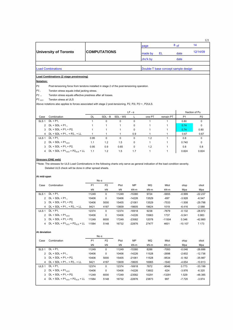
121

page 8 of 14


chc'k by date

Load Combinations Double-T base concept sample design

Load Combinations (2 stage prestressing)

Notation:


P1 i Tendon stress equals initial jacking stress.

P1 Tendon stress equals effective prestress after all losses.P1 ULS Tendon stress at ULS

Above notations also applies to forces associated with stage 2 post-tensioning, P2, P2i, P2 , P2ULS.

Case Combination DL SDL - B SDL - WS L one PT remain PT P1 P2

SLS 1 DL + P1i 1 0 0 0 1 1 0.80 0 2 DL + SDL + P1 1 1 1 0 1 1 0.74 0 3 DL + SDL + P1i + P2i 1 1 1 0 1 1 0.74 0.80 4 DL + SDL + P1 + P2 + LL 1 1 1 0.9 1 1 0.67 0.67ULS 1 DL + P1i 0.95 0 0 0 1.2 1 0.8 0 2 DL + SDL + P1ULS 1.1 1.2 1.5 0 1 1 0.740 0

3 DL + SDL + P1i + P2i 0.95 0.9 0.65 0 1.2 1 0.8 0.8

4 DL + SDL + P1ULS + P2ULS + LL 1.1 1.2 1.5 1.7 1 1 0.824 0.824

Stresses (ONE web)**Note: The stresses for ULS Load Combinations in the following charts only serve as general indication of the load condition severity. Detailed ULS check will be done in other spread sheets.

At mid-span

Case Combination P1 P2 Ptot MP MQ Mtot top bot

kN kN kN kN-m kN-m kN-m Mpa Mpa

SLS 1 DL + P1i 11249 0 11249 -15380 9724 -5655 -0.999 -22.237 2 DL + SDL + P1 10406 0 10406 -14226 13529 -697 -3.928 -6.547 3 DL + SDL + P1i + P2i 10406 5000 15405 -21061 13529 -7533 -1.508 -29.798 4 DL + SDL + P1 + P2 + LL 9421 4187 13609 -18605 19624 1019 -6.416 -2.588ULS 1 DL + P1i 12374 0 12374 -16918 9238 -7679 -0.132 -28.972 2 DL + SDL + P1ULS 10406 0 10406 -14226 15963 1737 -5.541 0.983 3 DL + SDL + P1i + P2i 11249 6000 17249 -23582 12078 -11504 0.346 -42.860 4 DL + SDL + P1ULS + P2ULS + LL 11584 5148 16732 -22876 27477 4601 -10.107 7.173

At deviation

Case Combination P1 P2 Ptot MP MQ Mtot top bot

kN kN kN kN-m kN-m kN-m Mpa Mpa

SLS 1 DL + P1i 11249 0 11249 -15380 8286 -7093 -0.046 -26.686 2 DL + SDL + P1 10406 0 10406 -14226 11528 -2698 -2.602 -12.736 3 DL + SDL + P1i + P2i 10406 5000 15405 -21061 11528 -9534 -0.182 -35.987 4 DL + SDL + P1 + P2 + LL 9421 4187 13609 -18605 16965 -1640 -4.654 -10.813ULS 1 DL + P1i 12374 0 12374 -16918 7872 -9046 0.773 -33.199 2 DL + SDL + P1ULS 10406 0 10406 -14226 13602 -624 -3.976 -6.320 3 DL + SDL + P1i + P2i 11249 6000 17249 -23582 10291 -13291 1.529 -48.385 4 DL + SDL + P1ULS + P2ULS + LL 11584 5148 16732 -22876 23873 997 -7.720 -3.974

fraction of Pu

No

No

LF -

122

page 9 of 14


chc'k by date

Short-term Prestress Losses Double-T base concept sample design

PT LayoutUse 78 strands Ap = 10920 mm2

CHBDC Table 8.5 (3) Min top cover = 120 mmCHBDC Table 8.5 (7) Min side cover = 80 mm

CHBDC CL 8.14.2.2.2 Min clear dist = 40 mmMin clear hor dist = 75 mm for precast segmental

Elevation Support Deviation Mid-span Deviation Supportx: Dist from left support [m] 0 11.30 18.3 25.3 36.60

Distance from cl PT to top of section [m] 1.075 1.72 1.720 1.72 1.075e: Dist btw cl tendon and cl section [m] 0.722 1.367 0.722

Mp = P e [kN-m]

PT total length = 37.635 mPT angle of inclination = 0.0546 rad.

Plan Support Deviation Mid-span Deviation Supportx: Dist from left support [m] 0 11.3 18.3 25.3 36.6

Distance from cl PT to cl web [m] 0.321 0.467 0.467 0.467 0.321

PT total length = 37.602 mPT angle of inclination = 0.0124 rad.

PT ForceAssume during jacking, fsj = 0.80 fpu = 1488 MpaStress at transfer - anchor = 1451 Mpa = 0.78 fpu

Stress at transfer - mid-span = 1426 MPa = 0.77 fpu

Loss of stage 1 prestress at 28 days = 50 Mpa = 0.03 fpuPrestress at 28 days at mid-span = 1376 MPa = 0.740 fpu

Assume eff. stress after all losses P = 0.67 fpu = 1246 MPa Adjust until assumed matches calculated.Calculated total losses at mid-span = 181 Mpa

Calculated final PT stress P = fsj - all losses = 1245 Mpa = 0.67 fpu

PT lossesFriction loss

Total angle change per deviation, = 0.067 rad.lower bound

Friction coefficients (AASHTO) K = 0 = 0.25

f (x) = fo { 1 - exp [ -Kx - (x) ] } = 24.7 Mpa

Anchor set lossAssume, set = 7 mm

Assume PT is anchored from one end.:. set = set / PT length = 0.0001860 mm/mm

ANC = set * Ep = 37.2 Mpa

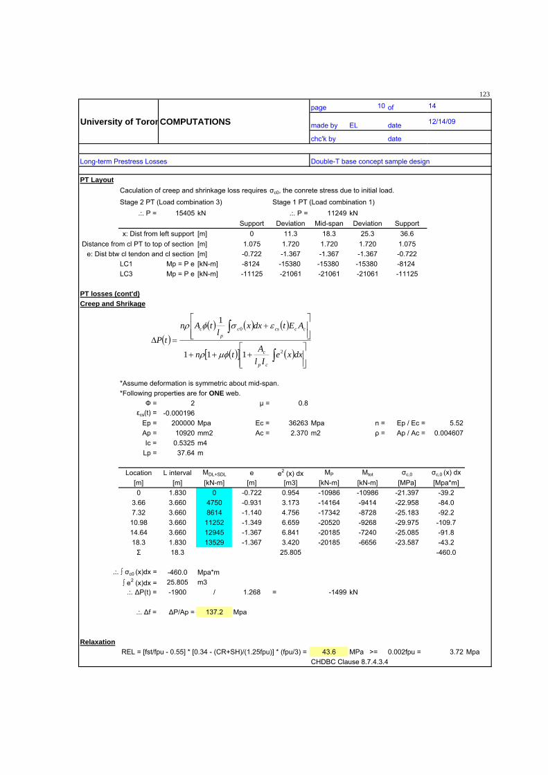
123

page 10 of 14

University of ToronCOMPUTATIONS made by EL date 12/14/09

chc'k by date

Long-term Prestress Losses Double-T base concept sample design

PT LayoutCaculation of creep and shrinkage loss requires c0, the conrete stress due to initial load.

Stage 2 PT (Load combination 3) Stage 1 PT (Load combination 1).:. P = 15405 kN .:. P = 11249 kN

Support Deviation Mid-span Deviation Supportx: Dist from left support [m] 0 11.3 18.3 25.3 36.6

Distance from cl PT to top of section [m] 1.075 1.720 1.720 1.720 1.075e: Dist btw cl tendon and cl section [m] -0.722 -1.367 -1.367 -1.367 -0.722

LC1 Mp = P e [kN-m] -8124 -15380 -15380 -15380 -8124LC3 Mp = P e [kN-m] -11125 -21061 -21061 -21061 -11125

PT losses (cont'd)Creep and Shrikage

*Assume deformation is symmetric about mid-span.*Following properties are for ONE web.

= 2 = 0.8cs(t) = -0.000196Ep = 200000 Mpa Ec = 36263 Mpa n = Ep / Ec = 5.52Ap = 10920 mm2 Ac = 2.370 m2 = Ap / Ac = 0.004607Ic = 0.5325 m4

Lp = 37.64 m

Location L interval MDL+SDL e e2 (x) dx MP Mtot c,0 c,0 (x) dx[m] [m] [kN-m] [m] [m3] [kN-m] [kN-m] [MPa] [Mpa*m]0 1.830 0 -0.722 0.954 -10986 -10986 -21.397 -39.2

3.66 3.660 4750 -0.931 3.173 -14164 -9414 -22.958 -84.07.32 3.660 8614 -1.140 4.756 -17342 -8728 -25.183 -92.210.98 3.660 11252 -1.349 6.659 -20520 -9268 -29.975 -109.714.64 3.660 12945 -1.367 6.841 -20185 -7240 -25.085 -91.818.3 1.830 13529 -1.367 3.420 -20185 -6656 -23.587 -43.2

18.3 25.805 -460.0

.:. c0 (x)dx = -460.0 Mpa*m e2 (x)dx = 25.805 m3.:. P(t) = -1900 / 1.268 = -1499 kN

.:. f = P/Ap = 137.2 Mpa

RelaxationREL = [fst/fpu - 0.55] * [0.34 - (CR+SH)/(1.25fpu)] * (fpu/3) = 43.6 MPa >= 0.002fpu = 3.72 Mpa

CHDBC Clause 8.7.4.3.4

dxxeIlA

tn

AEtdxxl

tAntP

cp

c

cccscp

c

2

0

111

1

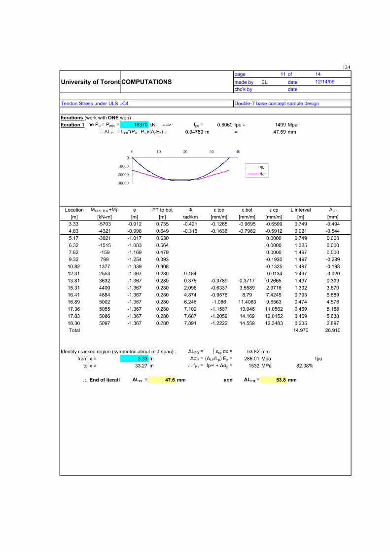
124page 11 of 14

University of Toront COMPUTATIONS made by EL date 12/14/09chc'k by date

Tendon Stress under ULS LC4 Double-T base concept sample design

Iterations (work with ONE web)Iteration 1 me P0 = Pmin = 16370 kN ==> fp0 = 0.8060 fpu = 1499 Mpa

.:. LPF = LP0*(P0 - P )/(ApEp) = 0.04759 m = 47.59 mm

Location MULS,TOT+Mp e PT to bot top bot cp L interval LP

[m] [kN-m] [m] [m] rad/km [mm/m] [mm/m] [mm/m] [m] [mm]3.33 -5703 -0.912 0.735 -0.421 -0.1265 -0.9695 -0.6599 0.749 -0.4944.83 -4321 -0.998 0.649 -0.316 -0.1636 -0.7962 -0.5912 0.921 -0.5445.17 -3021 -1.017 0.630 0.0000 0.749 0.0006.32 -1515 -1.083 0.564 0.0000 1.325 0.0007.82 -159 -1.169 0.479 0.0000 1.497 0.0009.32 799 -1.254 0.393 -0.1930 1.497 -0.28910.82 1377 -1.339 0.308 -0.1325 1.497 -0.19812.31 2553 -1.367 0.280 0.184 -0.0134 1.497 -0.02013.81 3632 -1.367 0.280 0.375 -0.3789 0.3717 0.2665 1.497 0.39915.31 4400 -1.367 0.280 2.096 -0.6337 3.5589 2.9716 1.302 3.87016.41 4884 -1.367 0.280 4.874 -0.9576 8.79 7.4245 0.793 5.88916.89 5002 -1.367 0.280 6.246 -1.086 11.4063 9.6563 0.474 4.57617.36 5055 -1.367 0.280 7.102 -1.1587 13.046 11.0562 0.469 5.18817.83 5086 -1.367 0.280 7.687 -1.2059 14.169 12.0152 0.469 5.63818.30 5097 -1.367 0.280 7.891 -1.2222 14.559 12.3483 0.235 2.897Total 14.970 26.910

Identify cracked region (symmetric about mid-span) : LPD = cp dx = 53.82 mmfrom x = 3.33 m P = ( LP/Lp) Ep = 286.01 Mpa fpu

to x = 33.27 m .:. fP1 = fp + p = 1532 MPa 82.38%

.:. End of iterati LPF = 47.6 mm and LPD = 53.8 mm

125

page 12 of 14


chc'k by date

Shear Double-T base concept sample design

ULS LC1 LC2 LC3 LC4Max Vp (ONE web) [kN] 655 568 941 913

max Vf-Vp (ONE web) = 2163 kNmax Vf-Vp (TWO web) = 4326 kN

dv = 0.72 h = 1440 mm sze = 300 mmApfp = 13609 kN

EpAp = 2184000 kNAssume EsAs = 0

Deviationdv 0.1L 0.2L 0.3L 0.4L

Vf kN 2896 2552 2070 1469 1070Mf/dv kN 2612 7196 12418 16823 18455

Mf/dv +Vf -Apfp kN -8100 -3861 880 4684 5917x 0 0 0 0 0

degree 29 29 30 37 380 0 0 0 0

Vc kN 1045 1045 803 401 345Vp kN 913 913 913 0 0

Vs = Vf-Vc-Vp kN 938 593 354 1069 725Av/s mm2/mm 1.003 0.634 0.401 1.526 1.111

s mm 398 630 997 262 359 min req 600mm

Shear forces (ONE web) - ULS LC1

VfVp

0 36.6


Vf

Vp

0 36.6


Vf

Vp

0 36.6


1518

Vf

913Vp

0 36.6

126page 13 of 14

University of Toronto COMPUTATIONS made by EL date 12/14/09chc'k by date

Shear Double-T base concept sample design

Shear Design according to CHBDC cl.8.9

At dv from supportmax Vf (ONE web) = 2896 kN At 1.6m from support (spread of anchor force)

Mf/dv = 2612 kN Use 2 legs of 20M at 180mm over 1.5m band.Mf/dv +Vf -Apfp = -8100 kN (per web)

x = 0 = 29 degrees = 0.40

Vc = 1045 kNVp = 913 kN

Vs = Vf-Vp-Vc = 938 kNAv/s required = 1.003 mm2/mm

Vf <= 0.125 cf'cbwdv+Vp = 3772 kNMinimum spacing from code

If use 15M bars, Av = 400 mm2 .:. s <= 398 mm 600 mmIf use 20M bars, Av = 600 mm2 .:. s <= 598 mm 600 mm

At 0.1L from supportmax Vf (ONE web) = 2552 kN

Mf/dv = 7196 kNMf/dv +Vf -Apfp = -3861 kN

x = 0 = 29 degrees = 0.40

Vc = 1045 kNVp = 913 kN





Mf/dv = 12418 kNMf/dv +Vf -Apfp = 880 kN

x = 0.000202 = 30.41059 degrees = 0.31

Vc = 803 kNVp = 913 kN




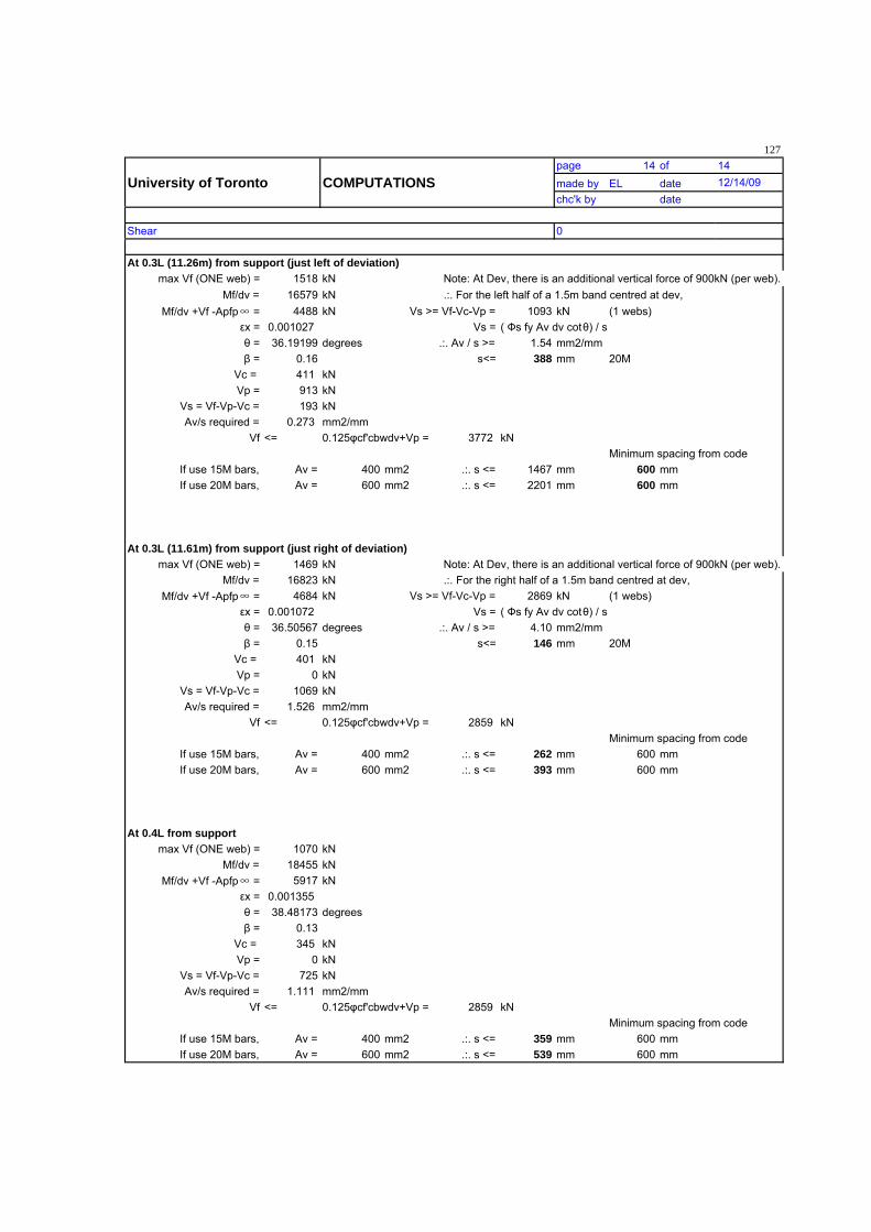
127page 14 of 14

University of Toronto COMPUTATIONS made by EL date 12/14/09chc'k by date

Shear 0

At 0.3L (11.26m) from support (just left of deviation)max Vf (ONE web) = 1518 kN Note: At Dev, there is an additional vertical force of 900kN (per web).

Mf/dv = 16579 kN .:. For the left half of a 1.5m band centred at dev,Mf/dv +Vf -Apfp = 4488 kN Vs >= Vf-Vc-Vp = 1093 kN (1 webs)

x = 0.001027 Vs = ( s fy Av dv cot ) / s = 36.19199 degrees .:. Av / s >= 1.54 mm2/mm = 0.16 s<= 388 mm 20M

Vc = 411 kNVp = 913 kN




At 0.3L (11.61m) from support (just right of deviation)max Vf (ONE web) = 1469 kN Note: At Dev, there is an additional vertical force of 900kN (per web).

Mf/dv = 16823 kN .:. For the right half of a 1.5m band centred at dev,Mf/dv +Vf -Apfp = 4684 kN Vs >= Vf-Vc-Vp = 2869 kN (1 webs)

x = 0.001072 Vs = ( s fy Av dv cot ) / s = 36.50567 degrees .:. Av / s >= 4.10 mm2/mm = 0.15 s<= 146 mm 20M

Vc = 401 kNVp = 0 kN





Mf/dv = 18455 kNMf/dv +Vf -Apfp = 5917 kN

x = 0.001355 = 38.48173 degrees = 0.13

Vc = 345 kNVp = 0 kN




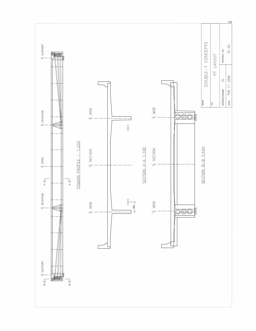
Appendix B:

CPCI Slab-on-Girder System Sample Calculations and Design

Drawings

138

139

page 1 of 11

COMPUTATIONS made by EL date 12/15/09

chc'k by date

Prestressed Concrete Girder Design - Structure: CPCI 1900 CPCI System Sample Design

Design Criteria

- Canadian Highway Bridge Design Code 2006 (CAN/CSA-S6-06) - refer to specific references listed

General Bridge Information

- Span No. 1 of 1 spans.

- Span length: 36600 mm Bridge Skew (rad.) = 0.00000- Adjacent span length 0 mm---> adjustments for continuity, L +: 36600 mm (Appendix A5.1) L -: 0 mm (Appendix A5.1)

- Deck width (travelled), Wc: 13.20 m

- No. of design lanes: 3 (ref. Table 3.8.2)

- Barrier wall area: 0.73 m2 2 barrier walls

- Total deck width: 13.80 m

- Deck thickness: 225 mm- Haunch thickness: 75 mm- Sidewalk width ; thickness: 0 mm 0 mm

- Total asphalt + w/p thickness: 90 mm- Spacing of girders: 2.35 m- Total no. of girders: 6- Top flange width 910 mm- Half deck span, BINT: 720 mm INTERIOR GIRDER- Half deck span, BEXT: 570 mm EXTERIOR GIRDER- Bearing Width = 300 mm- Deck overhang = 1.025 m < 0.5S

Effective Flange Width (cl. 5-8.2)

For Positive Moment Region

Interior (L+)/B ratio = 50.83 ===> Be = 720 mm .:. complete slab width is effectiveExterior (L+)/B ratio = 64.21 ===> Be = 570 mm .:. complete slab width is effective

For Negative Moment Region

Interior (L-)/B ratio = 0.00 ===> Be = 0 mmExterior (L-)/B ratio = 0.00 ===> Be = 0 mm

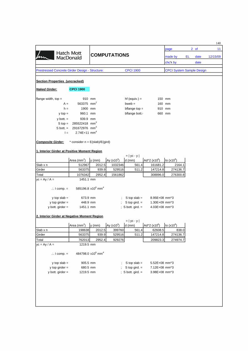
140

page 2 of 11


chc'k by date


Section Properties (uncracked)

Naked Girder: CPCI 1900

flange width, top = 910 mm hf (equiv.) = 150 mmA = 563375 mm2 bweb = 160 mmh = 1900 mm bflange top = 910 mm

y top = 960.1 mm bflange bott.= 660 mm

y bott. = 939.9 mmS top = 285522418 mm3

S bott. = 291672976 mm3

I = 2.74E+11 mm4

Composite Girder: * consider n = E(slab)/E(gird)

1. Interior Girder at Positive Moment Region = | yc - y |

Area (mm2) y (mm) Ay (x103) d (mm) Ad^2 (x106) Io (x106)Slab x n 512967 2012.5 1032346 561.4 161681.2 2164.1Girder 563375 939.9 529516 511.2 147214.8 274136.7

Total 1076342 2952.4 1561862 308896.0 276300.8yc = Ay / A = 1451.1 mm

.:. I comp. = 585196.8 x106 mm4

y top slab = 673.9 mm ; S top slab = 8.95E+08 mm^3y top girder = 448.9 mm ; S top gird. = 1.30E+09 mm^3

y bott. girder = 1451.1 mm ; S bott. gird. = 4.03E+08 mm^3

2. Interior Girder at Negative Moment Region = | yc - y |

Area (mm2) y (mm) Ay (x103) d (mm) Ad^2 (x106) Io (x106)Slab x n 198638 2012.5 399760 561.4 62608.5 838.0Girder 563375 939.9 529516 511.2 147214.8 274136.7

Total 762013 2952.4 929276 209823.3 274974.7yc = Ay / A = 1219.5 mm

.:. I comp. = 484798.0 x106 mm4

y top slab = 905.5 mm ; S top slab = 5.52E+08 mm^3y top girder = 680.5 mm ; S top gird. = 7.12E+08 mm^3

y bott. girder = 1219.5 mm ; S bott. gird. = 3.98E+08 mm^3

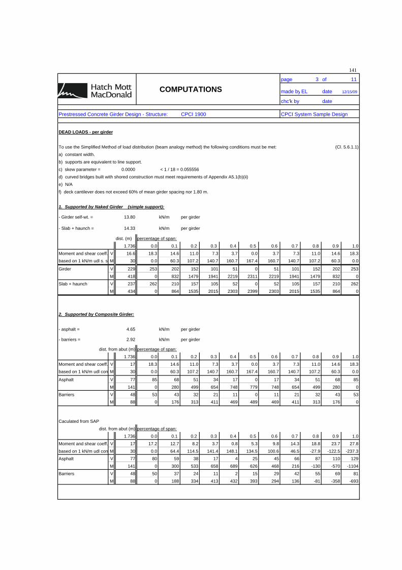
141

page 3 of 11


chc'k by date


DEAD LOADS - per girder

To use the Simplified Method of load distribution (beam analogy method) the following conditions must be met: (Cl. 5.6.1.1)

a) constant width.

b) supports are equivalent to line support.

c) skew parameter = 0.0000 < 1 / 18 = 0.055556

d) curved bridges built with shored construction must meet requirements of Appendix A5.1(b)(ii)

e) N/A

f) deck cantilever does not exceed 60% of mean girder spacing nor 1.80 m.

1. Supported by Naked Girder (simple support):

- Girder self-wt. = 13.80 kN/m per girder

- Slab + haunch = 14.33 kN/m per girder

dist. (m) percentage of span:

1.736 0.0 0.1 0.2 0.3 0.4 0.5 0.6 0.7 0.8 0.9 1.0

Moment and shear coeff. V 16.6 18.3 14.6 11.0 7.3 3.7 0.0 3.7 7.3 11.0 14.6 18.3based on 1 kN/m udl s. s M 30 0.0 60.3 107.2 140.7 160.7 167.4 160.7 140.7 107.2 60.3 0.0

Girder V 229 253 202 152 101 51 0 51 101 152 202 253

M 418 0 832 1479 1941 2219 2311 2219 1941 1479 832 0

Slab + haunch V 237 262 210 157 105 52 0 52 105 157 210 262M 434 0 864 1535 2015 2303 2399 2303 2015 1535 864 0

2. Supported by Composite Girder:

- asphalt = 4.65 kN/m per girder

- barriers = 2.92 kN/m per girder

dist. from abut (m) percentage of span:

1.736 0.0 0.1 0.2 0.3 0.4 0.5 0.6 0.7 0.8 0.9 1.0

Moment and shear coeff. V 17 18.3 14.6 11.0 7.3 3.7 0.0 3.7 7.3 11.0 14.6 18.3based on 1 kN/m udl con M 30 0.0 60.3 107.2 140.7 160.7 167.4 160.7 140.7 107.2 60.3 0.0

Asphalt V 77 85 68 51 34 17 0 17 34 51 68 85

M 141 0 280 499 654 748 779 748 654 499 280 0

Barriers V 48 53 43 32 21 11 0 11 21 32 43 53M 88 0 176 313 411 469 489 469 411 313 176 0

Caculated from SAP

dist. from abut (m) percentage of span:

1.736 0.0 0.1 0.2 0.3 0.4 0.5 0.6 0.7 0.8 0.9 1.0

Moment and shear coeff. V 17 17.2 12.7 8.2 3.7 0.8 5.3 9.8 14.3 18.8 23.7 27.8

based on 1 kN/m udl con M 30 0.0 64.4 114.5 141.4 148.1 134.5 100.6 46.5 -27.9 -122.5 -237.3

Asphalt V 77 80 59 38 17 4 25 45 66 87 110 129

M 141 0 300 533 658 689 626 468 216 -130 -570 -1104

Barriers V 48 50 37 24 11 2 15 29 42 55 69 81

M 88 0 188 334 413 432 393 294 136 -81 -358 -693

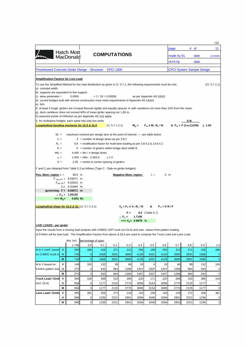
142

page 4 of 11


chc'k by date


Amplification Factors for Live Load

To use the Simplified Method for live load distribution as given in Cl. 5.7.1, the following requirements must be met: (Cl. 5.7.1.1)a) constant width.b) supports are equivalent to line support.c) skew parameter = 0.0000 < 1 / 18 = 0.05556 as per Appendix A5.1(b)(I)d) curved bridges built with shored construction must meet requirements of Appendix A5.1(b)(ii).e) N/Af) at least 3 longit. girders are of equal flexural rigidity and equally spaced, or with variations not more than 10% from the mean.g) deck cantilever does not exceed 60% of mean girder spacing nor 1.80 m.h) assumed points of inflection as per Appendix A5.1(a) apply.I) for multispine bridges, each spine has only two webs S NLongitudinal bending moments for ULS & SLS (cl. 5.7.1.2.1) Mg = Fm n MT RL / N & Fm = F (1+ Cf/100) > 1.05

MT = maximum moment per design lane at the point of interest ---- see table belown = 3 = number of design lanes as per 3.8.2

RL = 0.8 = modification factor for multi-lane loading as per 3.8.4.2 & 14.8.4.2N = 6 = number of girders within bridge deck width B

We = 4.400 = Wc / # design lanes= 1.000 = (We - 3.3)/0.6 < 1.0

S = 2.35 = centre to centre spacing of girders

F and Cf are obtained from Table 5.3 as follows (Type C - Slab-on-girder bridges):

Pos. Mom. region:L = 36.6 m Negative Mom. region: L = 0 mF tab EXT = 8.59071 m

Ftab INT= 9.02623 mCf= 9.31694 %

governing: F = 8.59071 m.:. Fm = 1.50142

==> Mg= 0.601 MT

Longitudinal shear for ULS & SLS(cl. 5.7.1.4.1) Vg = FV n VT RL / N & F V = S N / F

F = 8.2 (Table 5.7).:. FV = 1.7195 ==> Vg= 0.6878 VT

LIVE LOADS - per girderInput the results from a moving load analysis with CHBDC ONT truck (no DLA) and max. values from pattern loadingof 9 kN/m udl for lane load. The Amplification Factors from above & DLA are used to compute the Truck Load and Lane Load.

dist. (m) percentage of span:1.736 0.0 0.1 0.2 0.3 0.4 0.5 0.6 0.7 0.8 0.9 1.0

M & V coeff. based V 459 486 428 371 313 256 198 256 313 371 428 486on CHBDC truck (n M 743 0 1568 2831 3690 4128 4201 4128 3690 2831 1568 0

M 743 0 1568 2831 3690 4128 4201 4128 3690 2831 1568 0

M & V based on V 149 165 132 99 66 33 0 33 66 99 132 1659 kN/m pattern load M 272 0 543 964 1266 1447 1507 1447 1266 964 543 0

M 272 0 543 964 1266 1447 1507 1447 1266 964 543 0

Truck Load / Girde V 394 418 368 319 269 220 171 220 269 319 368 418(incl. DLA) M 558 0 1177 2125 2770 3099 3154 3099 2770 2125 1177 0

M 558 0 1177 2125 2770 3099 3154 3099 2770 2125 1177 0

Lane Load / Girde V 355 381 326 272 218 163 109 163 218 272 326 381M 596 0 1236 2221 2901 3266 3348 3266 2901 2221 1236 0

M 596 0 1236 2221 2901 3266 3348 3266 2901 2221 1236 0

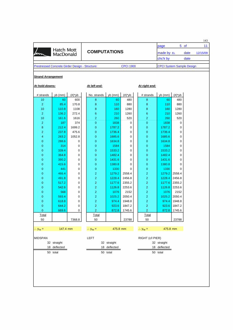
143

page 5 of 11


chc'k by date


Strand Arrangement

At hold-downs: At left end: At right end:

# strands yb (mm) (#)*yb No. strands yb (mm) (#)*yb # strands yb (mm) (#)*yb10 60 600 8 60 480 8 60 4802 85.4 170.8 8 110 880 8 110 880

10 110.8 1108 8 160 1280 8 160 12802 136.2 272.4 6 210 1260 6 210 1260

10 161.6 1616 2 260 520 2 260 5202 187 374 0 1838 0 0 1838 08 212.4 1699.2 0 1787.2 0 0 1787.2 02 237.8 475.6 0 1736.4 0 0 1736.4 04 263.2 1052.8 0 1685.6 0 0 1685.6 00 288.6 0 0 1634.8 0 0 1634.8 00 314 0 0 1584 0 0 1584 00 339.4 0 0 1533.2 0 0 1533.2 00 364.8 0 0 1482.4 0 0 1482.4 00 390.2 0 0 1431.6 0 0 1431.6 00 415.6 0 0 1380.8 0 0 1380.8 00 441 0 0 1330 0 0 1330 00 466.4 0 2 1279.2 2558.4 2 1279.2 2558.40 491.8 0 2 1228.4 2456.8 2 1228.4 2456.80 517.2 0 2 1177.6 2355.2 2 1177.6 2355.20 542.6 0 2 1126.8 2253.6 2 1126.8 2253.60 568 0 2 1076 2152 2 1076 21520 593.4 0 2 1025.2 2050.4 2 1025.2 2050.40 618.8 0 2 974.4 1948.8 2 974.4 1948.80 644.2 0 2 923.6 1847.2 2 923.6 1847.20 669.6 0 2 872.8 1745.6 2 872.8 1745.6

Total Total Total50 7368.8 50 23788 50 23788

.:. ybp = 147.4 mm .:. ybp = 475.8 mm .:. ybp = 475.8 mm

MIDSPAN LEFT RIGHT (c/l PIER)32 straight 32 straight 32 straight18 deflected 18 deflected 18 deflected

50 total 50 total 50 total

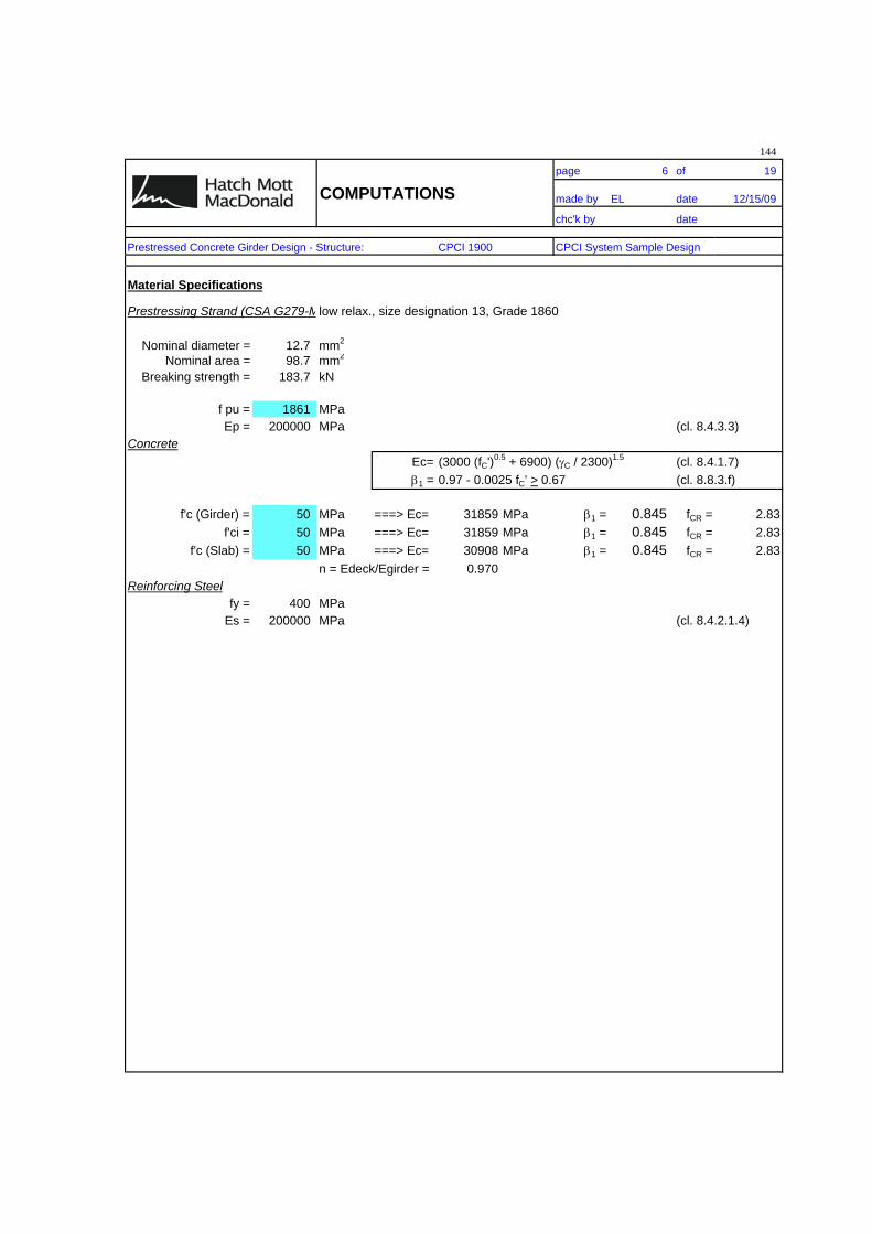
144

page 6 of 19


chc'k by date


Material Specifications

Prestressing Strand (CSA G279-Mlow relax., size designation 13, Grade 1860

Nominal diameter = 12.7 mm2

Nominal area = 98.7 mm2

Breaking strength = 183.7 kN

f pu = 1861 MPaEp = 200000 MPa (cl. 8.4.3.3)

Concrete Ec= (3000 (fC')0.5 + 6900) ( C / 2300)1.5 (cl. 8.4.1.7)

1 = 0.97 - 0.0025 fC' > 0.67 (cl. 8.8.3.f)

f'c (Girder) = 50 MPa ===> Ec= 31859 MPa 1 = 0.845 fCR = 2.83f'ci = 50 MPa ===> Ec= 31859 MPa 1 = 0.845 fCR = 2.83

f'c (Slab) = 50 MPa ===> Ec= 30908 MPa 1 = 0.845 fCR = 2.83n = Edeck/Egirder = 0.970

Reinforcing Steelfy = 400 MPa

Es = 200000 MPa (cl. 8.4.2.1.4)

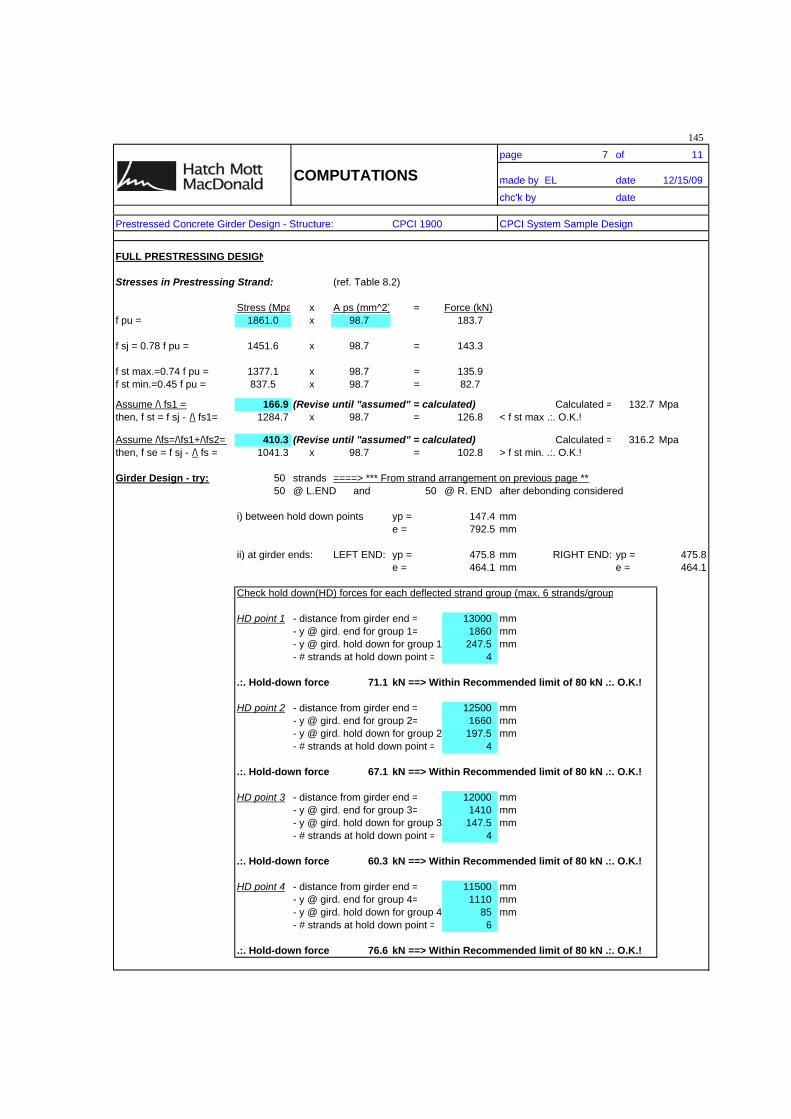
145

page 7 of 11


chc'k by date


FULL PRESTRESSING DESIGN

Stresses in Prestressing Strand: (ref. Table 8.2)

Stress (Mpa x A ps (mm^2) = Force (kN)f pu = 1861.0 x 98.7 183.7

f sj = 0.78 f pu = 1451.6 x 98.7 = 143.3

f st max.=0.74 f pu = 1377.1 x 98.7 = 135.9f st min.=0.45 f pu = 837.5 x 98.7 = 82.7

Assume /\ fs1 = 166.9 (Revise until "assumed" = calculated) Calculated = 132.7 Mpathen, f st = f sj - /\ fs1= 1284.7 x 98.7 = 126.8 < f st max .:. O.K.!

Assume /\fs=/\fs1+/\fs2= 410.3 (Revise until "assumed" = calculated) Calculated = 316.2 Mpathen, f se = f sj - /\ fs = 1041.3 x 98.7 = 102.8 > f st min. .:. O.K.!

Girder Design - try: 50 strands ====> *** From strand arrangement on previous page ***50 @ L.END and 50 @ R. END after debonding considered

i) between hold down points yp = 147.4 mme = 792.5 mm

ii) at girder ends: LEFT END: yp = 475.8 mm RIGHT END: yp = 475.8e = 464.1 mm e = 464.1

Check hold down(HD) forces for each deflected strand group (max. 6 strands/group

HD point 1 - distance from girder end = 13000 mm- y @ gird. end for group 1= 1860 mm- y @ gird. hold down for group 1 247.5 mm- # strands at hold down point = 4

.:. Hold-down force 71.1 kN ==> Within Recommended limit of 80 kN .:. O.K.!





HD point 4 - distance from girder end = 11500 mm- y @ gird. end for group 4= 1110 mm- y @ gird. hold down for group 4 85 mm- # strands at hold down point = 6


146

page 8 of 11


chc'k by date


CHECK ASSUMED LOSSES

1. Relaxation, REL1: (cl. 8.7.4.2.4)

Transfer assumed at t = 0.75 days (as per Comm. 8.7.4.2.4 for 24 hour production)

REL1 = log(24t)/45 * [fsj/fpy - 0.55] * fsj (Mpa) ; fpy = 0.9 fpu

= 12.8 MPa ; fsj = 0.78 fpu

For elastic shortening & creep calculations:

f cir = conc. stress @ c.g. prestress due to prestress at transfer + self-wt of member @ loc. of max. moment= [(Fst / Ag) + (Fst * e2) / I - (Md * e) / I]

e = e between hold downs = 0.793 mMd = M girder at midspan = 2311.2 kN-m

.:. f cir = 19.10 Mpa

f cds = conc. stress @ c.g. prestress due to all loads except dead load at transfer @ loc. of max. moment ("+" tensile)=Msl*e / Ig + Msdl*(yb - yp) / Icomp.

.:. f cds = 9.76 Mpa

2. Elastic Shortening, ES: (cl. 8.7.4.2.5)

ES = (Ep / E ci) * f cir= 119.9 MPa

.:. Total Losses At Transfer = fs1 = REL1 + ES = 132.7 Mpa

Stress in strand at transfer,fst = fsj - fs1

= 1319 Mpa < 0.74fPU OK (cl. C8.7.4.2.4)

Force per strand at transfer,Fst = 130 kN per strand

Total prestressing force at transfer,Fst = 6509 kN

147

page 9 of 11


chc'k by date


Confirm that As/Aps < 1.0. If not, a more detailed analysis is needed to calculate losses after transfer.3. Creep, CR: Mean relative humidity (H) = 70 % (Figure A3.1.3) (cl. 8.7.4.3.2)

Kcr = 2.0 for pretensioned design

CR = [ 1.37 - 0.77 * (0.01 * RH)2 ] * Kcr * (Ep/Ec) * (fcir - fcds) Where Ep = 200000 MPa= 116.4 MPa Ec = 31859 MPa

fcir = 19.1 MPafcds = 9.8 MPa

4. Shrinkage, SH: (cl. 8.7.4.3.3)

SH = 117.0 - 1.05 (RH) for pretensioned design= 43.5 MPa

5. Relaxation, REL2: (cl. 8.7.4.3.4)

REL2 = [(fst / fpu -0.55) * (0.34 - (CR + SH) / (1.25 * fpu)) * fpu / 3] > 0.002 * fpu= 23.6 MPa > 0.002*fpu OK

.:. fs2 = CR + SH + REL2 Total losses after transfer 183.5 MPa

.:. Total Losses at service loads = /\ fs = /\ fs1 + /\ fs2 316.2 Mpa

Stress in strand after all losses:fse = fsj - fs

1135 MPa > 0.45fpu OK

Force in strand after all losses:Fse = 1135(98.7)

112 kN

Total prestressing force after all losses:Fpe = 50(112)

5603 kN Approx. 22% final losses.

148

page 10 of 11


chc'k by date


STRESSES AT SLS AT CRITICAL LOCATIONS(effect of "K", differential shrinkage, to be considered separately)

1. At c/l girder: Total prestressing force after all losses,Fpe = 5603 kN (previous)

Item f top (Mpa) f bott. (Mpa) f slab (Mpa)- girder d.l. = 8.09 -7.92 --- Tension is - ve- slab+haunch d.l. = 8.40 -8.23 --- Compression is + ve- asphalt s.d.l. = 0.60 -1.93 0.87- barrier s.d.l. = 0.38 -1.21 0.55[f d.l. + f s.d.l.] = 17.47 -19.29 1.42

- 0.90 * live load = 2.31 -7.47 3.37[f d.l. + f s.d.l. + 0.9*f l.l.] = 19.78 -26.77 4.78

Fpe/Ag = 9.95 9.95 ---(Fpe x e)/S = -15.55 15.22 ---[f prestress] = -5.61 25.17 ---

[f d.l. + f s.d.l. + 0.9*f l.l. +f pr.] = 14.17 -1.60 4.78

Check Allowable Stresses: < < <fc' fcr = fc slab

50.00 -2.83 50.00 (cl. 8.8.4.6 & 8.12.4)O.K. O.K.! O.K.

2. At girder end 0.0 (Abutment):

Item f top (Mpa) f bott. (Mpa) f slab (Mpa)- girder d.l. = 0.00 0.00 ---- slab+haunch d.l. = 0.00 0.00 ---- asphalt s.d.l. = 0.00 0.00 0.00- barrier s.d.l. = 0.00 0.00 0.00[f d.l. + f s.d.l.] = 0.00 0.00 0.00

- 0.90 * live load = 0.00 0.00 0.00[f d.l. + f s.d.l. + 0.9*f l.l.] = 0.00 0.00 0.00

Fpe/Ag = 9.95 9.95 ---(Fpe x e)/S = -9.11 8.92 ---[f prestress] = 0.84 18.86 ---

[f d.l. + f s.d.l. + 0.75*f l.l. +f pr.] = 0.84 18.86 0.00

Check Allowable Stresses: < < <fc' fc' fc slab

50.00 50.00 50.00 (cl. 8.8.4.6 & 8.12.4)O.K. O.K. O.K.

149

page 11 of 11


chc'k by date


3. At girder end 1.0: (RIGHT END - Pier)

Itemf top

(Mpa)f bott.(Mpa)

f slab(Mpa)

- girder d.l. = 0.00 0.00 ---- slab+haunch d.l. = 0.00 0.00 ---- asphalt s.d.l. = 0.00 0.00 0.00- barrier s.d.l. = 0.00 0.00 0.00[f d.l. + f s.d.l.] = 0.00 0.00 0.00

- 0.90 * live load = 0.00 0.00 0.00[f d.l. + f s.d.l. + 0.9*f l.l.] = 0.00 0.00 0.00

Fpe/Ag = 9.95 9.95 ---(Fpe x e)/S = -9.11 8.92 ---[f prestress] = 0.84 18.86 ---

[f d.l. + f s.d.l. + 0.75*f l.l. +f pr.] = 0.84 18.86 0.00

Check Allowable Stresses: < < <fc' fc' fc slab

50.00 50.00 50.00 (cl. 8.8.4.6 & 8.12.4)O.K. O.K. O.K.

CHECK STRESSES AT SLS AT TRANSFER

Concrete Strength at Transfer = 50 Mpa

1. At hold-down points - I.e. at 1/3 span: M girder @ hold-dow 2032.9 kN-m (1/3 L along span)

Itemf top

(Mpa)f bott.(Mpa)

f girder = 7.12 -6.97

Fst/Ag = 11.55 11.55(Fst x e)/S = -18.07 17.68[f total] = 0.61 22.27

Check Allowable Stresses: < <0.6fci 0.6fci30.00 30.00 (cl. 8.8.4.6)O.K. O.K.

2. At ends: @ L. END (Abutment) @ R. END (Pier)

Itemf top

(Mpa)f bott.(Mpa)

f top(Mpa)

f bott.(Mpa)

Fst/Ag = 11.55 11.55 11.55 11.55(Fst x e)/S = -10.58 10.36 -10.58 10.36[f total] = 0.97 21.91 0.97 21.91

Check Allowable Stresses: < < < <0.6fci 0.6fci 0.6fci 0.6fci30.00 30.00 30.00 30.00O.K. O.K. O.K. O.K.

Appendix C:

Grillage Model Input File from SAP

152

SAP2000 v10.0.1 12/13/09 20:26:48

153

Table: Analysis Case Definitions

Case Type InitialCond ModalCase RunCase Text Text Text Text Yes/No

DEAD LinStatic Zero No MODAL LinModal Zero No

LC2 LinStatic Zero Yes LC3 LinStatic Zero Yes

Table: Case - Static 1 - Load Assignments

Case LoadType LoadName LoadSFText Text Text Unitless

DEAD Load case DEAD 1.000000LC2 Load case LC2-gravity 1.125000LC2 Load case LC2-torsion 1.125000LC3 Load case LC3-gravity 1.000000LC3 Load case LC3-torsion 1.000000

Table: Coordinate Systems

Name Type X Y Z AboutZ AboutY AboutXText Text m m m Degrees Degrees Degrees

GLOBAL Cartesian 0.00000 0.00000 0.00000 0.000 0.000 0.000 Table: Frame Loads - Point, Part 1 of 2

Frame LoadCase CoordSys Type Dir DistType RelDistText Text Text Text Text Text Unitless

2 LC3-gravity GLOBAL Force Gravity RelDist 0.22792 LC3-gravity GLOBAL Force Gravity RelDist 0.32622 LC3-gravity GLOBAL Force Gravity RelDist 0.35902 LC3-gravity GLOBAL Force Gravity RelDist 0.53932 LC3-gravity GLOBAL Force Gravity RelDist 0.71972 LC3-torsion GLOBAL Moment X RelDist 0.71972 LC3-torsion GLOBAL Moment X RelDist 0.22792 LC3-torsion GLOBAL Moment X RelDist 0.32622 LC3-torsion GLOBAL Moment X RelDist 0.35902 LC3-torsion GLOBAL Moment X RelDist 0.53935 LC2-gravity GLOBAL Force Gravity RelDist 0.22795 LC2-gravity GLOBAL Force Gravity RelDist 0.32625 LC2-gravity GLOBAL Force Gravity RelDist 0.35905 LC2-gravity GLOBAL Force Gravity RelDist 0.53935 LC3-gravity GLOBAL Force Gravity RelDist 0.22795 LC3-gravity GLOBAL Force Gravity RelDist 0.32625 LC3-gravity GLOBAL Force Gravity RelDist 0.35905 LC3-gravity GLOBAL Force Gravity RelDist 0.53935 LC3-gravity GLOBAL Force Gravity RelDist 0.71975 LC2-gravity GLOBAL Force Gravity RelDist 0.71975 LC2-torsion GLOBAL Moment X RelDist 0.71975 LC3-torsion GLOBAL Moment X RelDist 0.71975 LC2-torsion GLOBAL Moment X RelDist 0.22795 LC2-torsion GLOBAL Moment X RelDist 0.32625 LC2-torsion GLOBAL Moment X RelDist 0.35905 LC2-torsion GLOBAL Moment X RelDist 0.53935 LC3-torsion GLOBAL Moment X RelDist 0.22795 LC3-torsion GLOBAL Moment X RelDist 0.32625 LC3-torsion GLOBAL Moment X RelDist 0.35905 LC3-torsion GLOBAL Moment X RelDist 0.53931 LC2-gravity GLOBAL Force Gravity RelDist 0.22791 LC2-gravity GLOBAL Force Gravity RelDist 0.3262

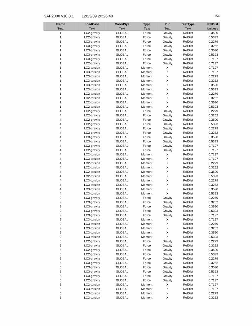
SAP2000 v10.0.1 12/13/09 20:26:48

154


1 LC2-gravity GLOBAL Force Gravity RelDist 0.35901 LC2-gravity GLOBAL Force Gravity RelDist 0.53931 LC3-gravity GLOBAL Force Gravity RelDist 0.22791 LC3-gravity GLOBAL Force Gravity RelDist 0.32621 LC3-gravity GLOBAL Force Gravity RelDist 0.35901 LC3-gravity GLOBAL Force Gravity RelDist 0.53931 LC3-gravity GLOBAL Force Gravity RelDist 0.71971 LC2-gravity GLOBAL Force Gravity RelDist 0.71971 LC2-torsion GLOBAL Moment X RelDist 0.71971 LC3-torsion GLOBAL Moment X RelDist 0.71971 LC3-torsion GLOBAL Moment X RelDist 0.22791 LC3-torsion GLOBAL Moment X RelDist 0.32621 LC3-torsion GLOBAL Moment X RelDist 0.35901 LC3-torsion GLOBAL Moment X RelDist 0.53931 LC2-torsion GLOBAL Moment X RelDist 0.22791 LC2-torsion GLOBAL Moment X RelDist 0.32621 LC2-torsion GLOBAL Moment X RelDist 0.35901 LC2-torsion GLOBAL Moment X RelDist 0.53934 LC2-gravity GLOBAL Force Gravity RelDist 0.22794 LC2-gravity GLOBAL Force Gravity RelDist 0.32624 LC2-gravity GLOBAL Force Gravity RelDist 0.35904 LC2-gravity GLOBAL Force Gravity RelDist 0.53934 LC3-gravity GLOBAL Force Gravity RelDist 0.22794 LC3-gravity GLOBAL Force Gravity RelDist 0.32624 LC3-gravity GLOBAL Force Gravity RelDist 0.35904 LC3-gravity GLOBAL Force Gravity RelDist 0.53934 LC3-gravity GLOBAL Force Gravity RelDist 0.71974 LC2-gravity GLOBAL Force Gravity RelDist 0.71974 LC2-torsion GLOBAL Moment X RelDist 0.71974 LC3-torsion GLOBAL Moment X RelDist 0.71974 LC2-torsion GLOBAL Moment X RelDist 0.22794 LC2-torsion GLOBAL Moment X RelDist 0.32624 LC2-torsion GLOBAL Moment X RelDist 0.35904 LC2-torsion GLOBAL Moment X RelDist 0.53934 LC3-torsion GLOBAL Moment X RelDist 0.22794 LC3-torsion GLOBAL Moment X RelDist 0.32624 LC3-torsion GLOBAL Moment X RelDist 0.35904 LC3-torsion GLOBAL Moment X RelDist 0.53939 LC3-gravity GLOBAL Force Gravity RelDist 0.22799 LC3-gravity GLOBAL Force Gravity RelDist 0.32629 LC3-gravity GLOBAL Force Gravity RelDist 0.35909 LC3-gravity GLOBAL Force Gravity RelDist 0.53939 LC3-gravity GLOBAL Force Gravity RelDist 0.71979 LC3-torsion GLOBAL Moment X RelDist 0.71979 LC3-torsion GLOBAL Moment X RelDist 0.22799 LC3-torsion GLOBAL Moment X RelDist 0.32629 LC3-torsion GLOBAL Moment X RelDist 0.35909 LC3-torsion GLOBAL Moment X RelDist 0.53936 LC2-gravity GLOBAL Force Gravity RelDist 0.22796 LC2-gravity GLOBAL Force Gravity RelDist 0.32626 LC2-gravity GLOBAL Force Gravity RelDist 0.35906 LC2-gravity GLOBAL Force Gravity RelDist 0.53936 LC3-gravity GLOBAL Force Gravity RelDist 0.22796 LC3-gravity GLOBAL Force Gravity RelDist 0.32626 LC3-gravity GLOBAL Force Gravity RelDist 0.35906 LC3-gravity GLOBAL Force Gravity RelDist 0.53936 LC3-gravity GLOBAL Force Gravity RelDist 0.71976 LC2-gravity GLOBAL Force Gravity RelDist 0.71976 LC2-torsion GLOBAL Moment X RelDist 0.71976 LC3-torsion GLOBAL Moment X RelDist 0.71976 LC3-torsion GLOBAL Moment X RelDist 0.22796 LC3-torsion GLOBAL Moment X RelDist 0.3262

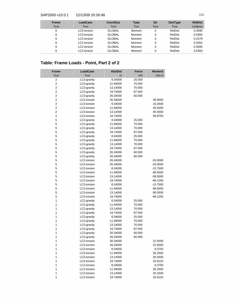
SAP2000 v10.0.1 12/13/09 20:26:48

155


6 LC3-torsion GLOBAL Moment X RelDist 0.35906 LC3-torsion GLOBAL Moment X RelDist 0.53936 LC2-torsion GLOBAL Moment X RelDist 0.22796 LC2-torsion GLOBAL Moment X RelDist 0.32626 LC2-torsion GLOBAL Moment X RelDist 0.35906 LC2-torsion GLOBAL Moment X RelDist 0.5393

Table: Frame Loads - Point, Part 2 of 2

Frame LoadCase AbsDist Force MomentText Text m KN KN-m

2 LC3-gravity 8.34000 25.0002 LC3-gravity 11.94000 70.0002 LC3-gravity 13.14000 70.0002 LC3-gravity 19.74000 87.5002 LC3-gravity 26.34000 60.0002 LC3-torsion 26.34000 39.00002 LC3-torsion 8.34000 16.25002 LC3-torsion 11.94000 45.50002 LC3-torsion 13.14000 45.50002 LC3-torsion 19.74000 56.87505 LC2-gravity 8.34000 25.0005 LC2-gravity 11.94000 70.0005 LC2-gravity 13.14000 70.0005 LC2-gravity 19.74000 87.5005 LC3-gravity 8.34000 25.0005 LC3-gravity 11.94000 70.0005 LC3-gravity 13.14000 70.0005 LC3-gravity 19.74000 87.5005 LC3-gravity 26.34000 60.0005 LC2-gravity 26.34000 60.0005 LC2-torsion 26.34000 -33.00005 LC3-torsion 26.34000 -33.00005 LC2-torsion 8.34000 -13.75005 LC2-torsion 11.94000 -38.50005 LC2-torsion 13.14000 -38.50005 LC2-torsion 19.74000 -48.12505 LC3-torsion 8.34000 -13.75005 LC3-torsion 11.94000 -38.50005 LC3-torsion 13.14000 -38.50005 LC3-torsion 19.74000 -48.12501 LC2-gravity 8.34000 25.0001 LC2-gravity 11.94000 70.0001 LC2-gravity 13.14000 70.0001 LC2-gravity 19.74000 87.5001 LC3-gravity 8.34000 25.0001 LC3-gravity 11.94000 70.0001 LC3-gravity 13.14000 70.0001 LC3-gravity 19.74000 87.5001 LC3-gravity 26.34000 60.0001 LC2-gravity 26.34000 60.0001 LC2-torsion 26.34000 22.50001 LC3-torsion 26.34000 22.50001 LC3-torsion 8.34000 9.37501 LC3-torsion 11.94000 26.25001 LC3-torsion 13.14000 26.25001 LC3-torsion 19.74000 32.81251 LC2-torsion 8.34000 9.37501 LC2-torsion 11.94000 26.25001 LC2-torsion 13.14000 26.25001 LC2-torsion 19.74000 32.8125

SAP2000 v10.0.1 12/13/09 20:26:48

156

Frame LoadCase AbsDist Force MomentText Text m KN KN-m

4 LC2-gravity 8.34000 25.0004 LC2-gravity 11.94000 70.0004 LC2-gravity 13.14000 70.0004 LC2-gravity 19.74000 87.5004 LC3-gravity 8.34000 25.0004 LC3-gravity 11.94000 70.0004 LC3-gravity 13.14000 70.0004 LC3-gravity 19.74000 87.5004 LC3-gravity 26.34000 60.0004 LC2-gravity 26.34000 60.0004 LC2-torsion 26.34000 12.00004 LC3-torsion 26.34000 12.00004 LC2-torsion 8.34000 5.00004 LC2-torsion 11.94000 14.00004 LC2-torsion 13.14000 14.00004 LC2-torsion 19.74000 17.50004 LC3-torsion 8.34000 5.00004 LC3-torsion 11.94000 14.00004 LC3-torsion 13.14000 14.00004 LC3-torsion 19.74000 17.50009 LC3-gravity 8.34000 25.0009 LC3-gravity 11.94000 70.0009 LC3-gravity 13.14000 70.0009 LC3-gravity 19.74000 87.5009 LC3-gravity 26.34000 60.0009 LC3-torsion 26.34000 49.50009 LC3-torsion 8.34000 20.62509 LC3-torsion 11.94000 57.75009 LC3-torsion 13.14000 57.75009 LC3-torsion 19.74000 72.18756 LC2-gravity 8.34000 25.0006 LC2-gravity 11.94000 70.0006 LC2-gravity 13.14000 70.0006 LC2-gravity 19.74000 87.5006 LC3-gravity 8.34000 25.0006 LC3-gravity 11.94000 70.0006 LC3-gravity 13.14000 70.0006 LC3-gravity 19.74000 87.5006 LC3-gravity 26.34000 60.0006 LC2-gravity 26.34000 60.0006 LC2-torsion 26.34000 -22.87506 LC3-torsion 26.34000 -22.87506 LC3-torsion 8.34000 -9.53136 LC3-torsion 11.94000 -26.68756 LC3-torsion 13.14000 -26.68756 LC3-torsion 19.74000 -33.35946 LC2-torsion 8.34000 -9.53136 LC2-torsion 11.94000 -26.68756 LC2-torsion 13.14000 -26.68756 LC2-torsion 19.74000 -33.3594

Table: Frame Section Assignments

Frame SectionType AutoSelect AnalSect DesignSect MatProp Text Text Text Text Text Text

1 Rectangular N.A. NLONGR N.A. Default 2 Tee N.A. NLONGT NLONGT Default 3 Tee N.A. NTRANSE NTRANSE Default 4 Rectangular N.A. NLONGR N.A. Default 5 Tee N.A. NLONGT NLONGT Default 6 Rectangular N.A. NLONGR N.A. Default

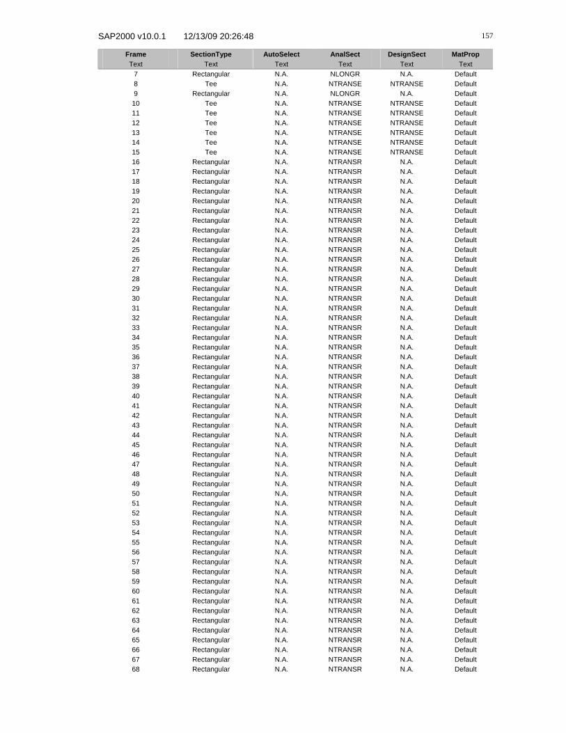
SAP2000 v10.0.1 12/13/09 20:26:48

157

Frame SectionType AutoSelect AnalSect DesignSect MatProp Text Text Text Text Text Text

7 Rectangular N.A. NLONGR N.A. Default 8 Tee N.A. NTRANSE NTRANSE Default 9 Rectangular N.A. NLONGR N.A. Default

10 Tee N.A. NTRANSE NTRANSE Default 11 Tee N.A. NTRANSE NTRANSE Default 12 Tee N.A. NTRANSE NTRANSE Default 13 Tee N.A. NTRANSE NTRANSE Default 14 Tee N.A. NTRANSE NTRANSE Default 15 Tee N.A. NTRANSE NTRANSE Default 16 Rectangular N.A. NTRANSR N.A. Default 17 Rectangular N.A. NTRANSR N.A. Default 18 Rectangular N.A. NTRANSR N.A. Default 19 Rectangular N.A. NTRANSR N.A. Default 20 Rectangular N.A. NTRANSR N.A. Default 21 Rectangular N.A. NTRANSR N.A. Default 22 Rectangular N.A. NTRANSR N.A. Default 23 Rectangular N.A. NTRANSR N.A. Default 24 Rectangular N.A. NTRANSR N.A. Default 25 Rectangular N.A. NTRANSR N.A. Default 26 Rectangular N.A. NTRANSR N.A. Default 27 Rectangular N.A. NTRANSR N.A. Default 28 Rectangular N.A. NTRANSR N.A. Default 29 Rectangular N.A. NTRANSR N.A. Default 30 Rectangular N.A. NTRANSR N.A. Default 31 Rectangular N.A. NTRANSR N.A. Default 32 Rectangular N.A. NTRANSR N.A. Default 33 Rectangular N.A. NTRANSR N.A. Default 34 Rectangular N.A. NTRANSR N.A. Default 35 Rectangular N.A. NTRANSR N.A. Default 36 Rectangular N.A. NTRANSR N.A. Default 37 Rectangular N.A. NTRANSR N.A. Default 38 Rectangular N.A. NTRANSR N.A. Default 39 Rectangular N.A. NTRANSR N.A. Default 40 Rectangular N.A. NTRANSR N.A. Default 41 Rectangular N.A. NTRANSR N.A. Default 42 Rectangular N.A. NTRANSR N.A. Default 43 Rectangular N.A. NTRANSR N.A. Default 44 Rectangular N.A. NTRANSR N.A. Default 45 Rectangular N.A. NTRANSR N.A. Default 46 Rectangular N.A. NTRANSR N.A. Default 47 Rectangular N.A. NTRANSR N.A. Default 48 Rectangular N.A. NTRANSR N.A. Default 49 Rectangular N.A. NTRANSR N.A. Default 50 Rectangular N.A. NTRANSR N.A. Default 51 Rectangular N.A. NTRANSR N.A. Default 52 Rectangular N.A. NTRANSR N.A. Default 53 Rectangular N.A. NTRANSR N.A. Default 54 Rectangular N.A. NTRANSR N.A. Default 55 Rectangular N.A. NTRANSR N.A. Default 56 Rectangular N.A. NTRANSR N.A. Default 57 Rectangular N.A. NTRANSR N.A. Default 58 Rectangular N.A. NTRANSR N.A. Default 59 Rectangular N.A. NTRANSR N.A. Default 60 Rectangular N.A. NTRANSR N.A. Default 61 Rectangular N.A. NTRANSR N.A. Default 62 Rectangular N.A. NTRANSR N.A. Default 63 Rectangular N.A. NTRANSR N.A. Default 64 Rectangular N.A. NTRANSR N.A. Default 65 Rectangular N.A. NTRANSR N.A. Default 66 Rectangular N.A. NTRANSR N.A. Default 67 Rectangular N.A. NTRANSR N.A. Default 68 Rectangular N.A. NTRANSR N.A. Default

SAP2000 v10.0.1 12/13/09 20:26:48

158

Frame SectionType AutoSelect AnalSect DesignSect MatProp Text Text Text Text Text Text 69 Rectangular N.A. NTRANSR N.A. Default 70 Rectangular N.A. NTRANSR N.A. Default 71 Rectangular N.A. NTRANSR N.A. Default 72 Rectangular N.A. NTRANSR N.A. Default 73 Rectangular N.A. NTRANSR N.A. Default 74 Rectangular N.A. NTRANSR N.A. Default 75 Rectangular N.A. NTRANSR N.A. Default 76 Rectangular N.A. NTRANSR N.A. Default 77 Rectangular N.A. NTRANSR N.A. Default 78 Rectangular N.A. NTRANSR N.A. Default 79 Rectangular N.A. NTRANSR N.A. Default 80 Rectangular N.A. NTRANSR N.A. Default 81 Rectangular N.A. NTRANSR N.A. Default 82 Rectangular N.A. NTRANSR N.A. Default 83 Rectangular N.A. NTRANSR N.A. Default 84 I/Wide Flange N.A. NTRANSD N.A. Default 85 I/Wide Flange N.A. NTRANSD N.A. Default 86 I/Wide Flange N.A. NTRANSD N.A. Default 87 I/Wide Flange N.A. NTRANSD N.A. Default 88 I/Wide Flange N.A. NTRANSD N.A. Default 89 I/Wide Flange N.A. NTRANSD N.A. Default 90 Rectangular N.A. NTRANSR N.A. Default 91 Rectangular N.A. NTRANSR N.A. Default 92 Rectangular N.A. NTRANSR N.A. Default 93 Rectangular N.A. NTRANSR N.A. Default 94 Rectangular N.A. NTRANSR N.A. Default 95 Rectangular N.A. NTRANSR N.A. Default 96 Rectangular N.A. NTRANSR N.A. Default 97 Rectangular N.A. NTRANSR N.A. Default 98 Rectangular N.A. NTRANSR N.A. Default 99 Rectangular N.A. NTRANSR N.A. Default

100 Rectangular N.A. NTRANSR N.A. Default 101 Rectangular N.A. NTRANSR N.A. Default 102 Rectangular N.A. NTRANSR N.A. Default 103 Rectangular N.A. NTRANSR N.A. Default 104 Rectangular N.A. NTRANSR N.A. Default 105 Rectangular N.A. NTRANSR N.A. Default 106 Rectangular N.A. NTRANSR N.A. Default 107 Rectangular N.A. NTRANSR N.A. Default 108 Rectangular N.A. NTRANSR N.A. Default 109 Rectangular N.A. NTRANSR N.A. Default 110 Rectangular N.A. NTRANSR N.A. Default 111 Rectangular N.A. NTRANSR N.A. Default 112 Rectangular N.A. NTRANSR N.A. Default 113 Rectangular N.A. NTRANSR N.A. Default 114 Rectangular N.A. NTRANSR N.A. Default 115 Rectangular N.A. NTRANSR N.A. Default 116 Rectangular N.A. NTRANSR N.A. Default 117 Rectangular N.A. NTRANSR N.A. Default 118 Rectangular N.A. NTRANSR N.A. Default 119 Rectangular N.A. NTRANSR N.A. Default 120 Rectangular N.A. NTRANSR N.A. Default 121 Rectangular N.A. NTRANSR N.A. Default 122 Rectangular N.A. NTRANSR N.A. Default 123 Rectangular N.A. NTRANSR N.A. Default 124 I/Wide Flange N.A. NTRANSD N.A. Default 125 I/Wide Flange N.A. NTRANSD N.A. Default 126 I/Wide Flange N.A. NTRANSD N.A. Default 127 I/Wide Flange N.A. NTRANSD N.A. Default 128 I/Wide Flange N.A. NTRANSD N.A. Default 129 I/Wide Flange N.A. NTRANSD N.A. Default 130 Rectangular N.A. NTRANSR N.A. Default

SAP2000 v10.0.1 12/13/09 20:26:48

159

Frame SectionType AutoSelect AnalSect DesignSect MatProp Text Text Text Text Text Text 131 Rectangular N.A. NTRANSR N.A. Default 132 Rectangular N.A. NTRANSR N.A. Default 133 Rectangular N.A. NTRANSR N.A. Default 134 Rectangular N.A. NTRANSR N.A. Default 135 Rectangular N.A. NTRANSR N.A. Default 136 Rectangular N.A. NTRANSR N.A. Default 137 Rectangular N.A. NTRANSR N.A. Default 138 Rectangular N.A. NTRANSR N.A. Default 139 Rectangular N.A. NTRANSR N.A. Default 140 Rectangular N.A. NTRANSR N.A. Default 141 Rectangular N.A. NTRANSR N.A. Default 142 Rectangular N.A. NTRANSR N.A. Default 143 Rectangular N.A. NTRANSR N.A. Default 144 Rectangular N.A. NTRANSR N.A. Default 145 Rectangular N.A. NTRANSR N.A. Default 146 Rectangular N.A. NTRANSR N.A. Default 147 Rectangular N.A. NTRANSR N.A. Default 148 Rectangular N.A. NTRANSR N.A. Default 149 Rectangular N.A. NTRANSR N.A. Default 150 Rectangular N.A. NTRANSR N.A. Default 151 Rectangular N.A. NTRANSR N.A. Default 152 Rectangular N.A. NTRANSR N.A. Default 153 Rectangular N.A. NTRANSR N.A. Default 154 Tee N.A. NTRANSE NTRANSE Default 155 Tee N.A. NTRANSE NTRANSE Default 156 Tee N.A. NTRANSE NTRANSE Default 157 Tee N.A. NTRANSE NTRANSE Default

Table: Frame Section Properties 01 - General, Part 1 of 6

SectionName Material Shape t3 t2 tf twText Text Text m m m m

NLONGR OTHER Rectangular 0.225000 1.975000 NLONGT CONC Tee 2.000000 1.975000 0.343500 0.297500

NTRANSD CONC I/Wide Flange 2.000000 1.525000 0.273000 0.300000NTRANSE CONC Tee 2.000000 1.525000 0.273000 0.600000NTRANSR OTHER Rectangular 0.273000 1.525000


SectionName t2b tfb Area TorsConst I33 I22 AS2Text m m m2 m4 m4 m4 m2

NLONGR 0.444375 0.006961 0.001875 0.144445 0.370313NLONGT 1.171221 0.039284 0.404811 0.224154 0.595000

NTRANSD 1.100000 0.504000 1.337625 0.051874 0.685439 0.139338 0.600000NTRANSE 1.452525 0.128758 0.557124 0.111771 1.200000NTRANSR 0.416325 0.009176 0.002586 0.080685 0.346938


SectionName AS3 S33 S22 Z33 Z22 R33 R22Text m2 m3 m3 m3 m3 m m

NLONGR 0.370313 0.016664 0.146273 0.024996 0.219410 0.064952 0.570133NLONGT 0.565344 0.287613 0.226992 0.520326 0.371619 0.587905 0.437476

NTRANSD 0.808938 0.678933 0.182739 0.886428 0.338701 0.715842 0.322751NTRANSE 0.346938 0.484405 0.146584 0.791485 0.314154 0.619319 0.277397NTRANSR 0.346938 0.018943 0.105816 0.028414 0.158724 0.078808 0.440230

SAP2000 v10.0.1 12/13/09 20:26:48

160


SectionName ConcCol ConcBeam Color TotalWt TotalMass FromFile AModText Yes/No Yes/No Text KN KN-s2/m Yes/No Unitless

NLONGR No No Blue 1916.045 195.22 No 1.000000NLONGT No Yes Blue 2020.146 206.00 No 1.000000

NTRANSD No No Magenta 746.203 76.09 No 1.000000NTRANSE No Yes White 810.301 82.63 No 1.000000NTRANSR No No Blue 2438.467 248.45 No 1.000000

Table: Grid Lines, Part 1 of 2

CoordSys AxisDir GridID XRYZCoord LineType LineColor Visible BubbleLocText Text Text m Text Text Yes/No Text

GLOBAL X x1 0.00000 Primary Gray8Dark Yes End GLOBAL X x2 1.52500 Primary Gray8Dark Yes End GLOBAL X x3 3.05000 Primary Gray8Dark Yes End GLOBAL X x4 4.57500 Primary Gray8Dark Yes End GLOBAL X x5 6.10000 Primary Gray8Dark Yes End GLOBAL X x6 7.62500 Primary Gray8Dark Yes End GLOBAL X x7 9.15000 Primary Gray8Dark Yes End GLOBAL X x8 10.67500 Primary Gray8Dark Yes End GLOBAL X x9 12.20000 Primary Gray8Dark Yes End GLOBAL X x10 13.72500 Primary Gray8Dark Yes End GLOBAL X x11 15.25000 Primary Gray8Dark Yes End GLOBAL X x12 16.77500 Primary Gray8Dark Yes End GLOBAL X x13 18.30000 Primary Gray8Dark Yes End GLOBAL X x14 19.82500 Primary Gray8Dark Yes End GLOBAL X x15 21.35000 Primary Gray8Dark Yes End GLOBAL X x16 22.87500 Primary Gray8Dark Yes End GLOBAL X x17 24.40000 Primary Gray8Dark Yes End GLOBAL X x18 25.92500 Primary Gray8Dark Yes End GLOBAL X x19 27.45000 Primary Gray8Dark Yes End GLOBAL X x20 28.97500 Primary Gray8Dark Yes End GLOBAL X x21 30.50000 Primary Gray8Dark Yes End GLOBAL X x22 32.02500 Primary Gray8Dark Yes End GLOBAL X x23 33.55000 Primary Gray8Dark Yes End GLOBAL X x24 35.07500 Primary Gray8Dark Yes End GLOBAL X x25 36.60000 Primary Gray8Dark Yes End GLOBAL Y y1 -1.96875 Primary Gray8Dark Yes End GLOBAL Y y2 0.00000 Primary Gray8Dark Yes End GLOBAL Y y3 1.97500 Primary Gray8Dark Yes End GLOBAL Y y4 3.95000 Primary Gray8Dark Yes End GLOBAL Y y5 5.92500 Primary Gray8Dark Yes End GLOBAL Y y6 7.90000 Primary Gray8Dark Yes End GLOBAL Y y7 9.86875 Primary Gray8Dark Yes End GLOBAL Z z1 0.00000 Primary Gray8Dark Yes End

Table: Load Case Definitions

LoadCase DesignType SelfWtMult AutoLoad Text Text Unitless Text

LC2-gravity LIVE 0.000000 LC2-torsion LIVE 0.000000 LC3-gravity LIVE 0.000000 LC3-torsion LIVE 0.000000

SAP2000 v10.0.1 12/13/09 20:26:48

161

Table: Program Control, Part 1 of 2

ProgramName

Version ProgLevel LicenseOS LicenseSC LicenseBR LicenseHT CurrUnits

Text Text Text Yes/No Yes/No Yes/No Yes/No Text SAP2000 10.0.1 Advanced Yes Yes Yes No KN, m, C

Documents

Bridge System with Precast Concrete Double-T Girder and External Unbonded Post-tensioning