ISSN 2042-2695

CEP Discussion Paper No 960

December 2009

Do Oil Windfalls Improve Living Standards? Evidence from Brazil

Francesco Caselli and Guy Michaels

Abstract We use variation in oil output among Brazilian municipalities to investigate the effects of resource windfalls. We find muted effects of oil through market channels: offshore oil has no effect on municipal non-oil GDP or its composition, while onshore oil has only modest effects on non-oil GDP composition. However, oil abundance causes municipal revenues and reported spending on a range of budgetary items to increase, mainly as a result of royalties paid by Petrobras. Nevertheless, survey-based measures of social transfers, public good provision, infrastructure, and household income increase less (if at all) than one might expect given the increase in reported spending. To explain why oil windfalls contribute little to local living standards, we use data from the Brazilian media and federal police to document that very large oil output increases alleged instances of illegal activities associated with mayors. Keywords: Brazil, corruption, Dutch disease, fiscal windfalls, natural resources and oil JEL Classifications: E02, E62, H11, H40, H71, H72, H75, H76, O11, O13, O32, O33 This paper was produced as part of the Centre’s Macro Programme. The Centre for Economic Performance is financed by the Economic and Social Research Council. Acknowledgements We are grateful to Facundo Alvaredo, Igor Barenboim, Gadi Barlevy, Marianne Bertrand, Irineu de Carvalho, Fred Finan, Doug Gollin, Todd Gormley, Steve Haber, Seema Jayachandran, Martin Koppensteiner, Andrei Levchenko, Marco Manacorda, Alan Manning, Halvor Mehlum, Marcos Mendes, Benoit Mojon, Steve Pischke, Steve Redding, Eustachio Reis, Silvana Tenreyro, Adrian Wood, and Alwyn Young for comments, data, or both; useful comments were also received from seminar participants at Brown, Bruegel, Columbia, INSEAD, LSE, Oxford, Sussex, Toronto, Yale, and Zurich; conference participants at AMID/BREAD/CEPR 2009, Development Conference at NYU, ESSIM 2009, OxCarre 2008, NBER Growth Conference in San Francisco, and NBER Summer Institute Political Economy Workshop. We thank Gabriela Domingues, Renata Narita, and Gunes Asik-Altintas for research assistance. Francesco Caselli gratefully acknowledges the support of CEP, ESRC and Banco de España, the latter through the Banco de España Professorship. Francesco Caselli is a Programme Director at the Centre for Economic Performance and Professor of Economics, London School of Economics. He is also Banco de España Visiting Professor, CREI and a Research Fellow with CEPR and NBER. Guy Michaels is a Research Associate for the Centre for Economic Performance and Lecturer in the Department of Economics, London School of Economics. He is also a Research Affiliate with CEPR. Published by Centre for Economic Performance London School of Economics and Political Science Houghton Street London WC2A 2AE All rights reserved. No part of this publication may be reproduced, stored in a retrieval system or transmitted in any form or by any means without the prior permission in writing of the publisher nor be issued to the public or circulated in any form other than that in which it is published. Requests for permission to reproduce any article or part of the Working Paper should be sent to the editor at the above address. © F. Caselli and G. Michaels, submitted 2009

I. Introduction Should communities that discover oil in their subsoil or off their coast, rejoice or mourn? Should citizens be thrilled or worried when their governments receive fiscal windfalls? Ample anecdotal evidence on both questions has, over the years, shaken many economists’ confidence that the answer is as obvious (rejoice, of course) as it might seem at first brush. Oil, like many other natural resources, is increasingly suspected of being a “curse,” bringing Dutch Disease, corruption, rent seeking, and other ills that result in the dissipation of most possible benefits – if not in extreme cases in an outright decline in living standards. Fiscal windfalls, such as international aid or – in the case of local government – transfers from the central government, also stand often accused of creating a similar set of problems. And when oil abundance generates royalties for the government there is scope for a potentially particularly lethal mix where all the problems allegedly intrinsic to resource abundance are compounded by those thought to be associated with the fiscal windfall. Brazilian municipalities offer an interesting testing ground for these conjectures. Oil endowments, and hence production, vary widely among them, and we argue that conditional on a few geographic controls this variation is exogenous to municipal characteristics. Hence, we can ask whether oil has positive or negative spillovers on other market activities. Furthermore, oil-producing municipalities are entitled to royalties, so we can investigate the consequences of an oil-related fiscal windfall. We begin by investigating the effects of oil through market spillovers, and find that these are small. In particular, in the cross-section of Brazilian municipalities one Real of extra value added from oil translates into roughly one Real of aggregate GDP, indicating that to a first approximation oil production has no spillovers (either negative or positive) on non-oil activities. We do find some small changes in the composition of non-oil GDP when the oil is located onshore (manufacturing shrinks and services expand), but not when it is offshore. We next turn to the fiscal windfall. We confirm that municipal revenues increase significantly with oil production, and that the bulk of this increase is accounted for by royalties. Evidently, royalty payments are not undone by offsetting changes in other transfers from the state or federal governments (or by tax cuts). The revenue-side expansion is matched by a corresponding increase in the expenditure-side of the budget. Municipalities that receive oil windfalls report significant increases in spending on a variety of public goods and services, such as housing and urban infrastructure, education, health, and transportation, and in transfers to households. Given the significant expansion in reported spending, one would expect sizable improvements in welfare-relevant outcomes for the local population. We therefore look at measures of housing quality and quantity, supply of educational and health inputs, road infrastructure, and welfare receipts. The results paint a complex picture, with no apparent changes in some areas, small improvements in some others, and small worsening in others yet. On balance, however, the data appear to suggest that the actual flow of goods, services, and transfers to the population is not quite commensurate to the reported spending increases stemming from the windfall, a shortfall that we dub “missing money.” To confirm that the windfall does not trickle down to the population through other channels we look at household income, and find only minimal

2

improvements. We also show that oil-rich municipalities did not experience a differential increase in population. This implies that our results are not driven by a dilution of the benefits of oil abundance. Furthermore, the fact that people do not flock to oil-abundant communities reinforces our message that oil abundance has not been seen as particularly beneficial by the population. Our finding that oil windfalls translate into little improvement in the provision of public goods or the population’s living standards raises an important question: where are the oil revenues going? To partly address this question we put together a few pieces of tentative evidence. First, oil revenues increase the size of municipal workers’ houses (but not the size of other residents’ houses). Second, Brazil’s news agency is more likely to carry news items mentioning corruption and the mayor in municipalities with very high levels of oil output (on an absolute, though not per capita, basis). Third, federal police operations are more likely to occur in municipalities with very high levels of oil output (again in absolute terms). And finally, we document anecdotal evidence of scandals involving mayors in several of the largest oil producing municipalities, some of which involve large sums of money. To partly explain why senior municipal workers may have thought that they could “get away” with large-scale alleged theft in a country where local elections are held regularly, we note that a survey in the largest oil producing municipality found considerable ignorance among residents regarding the scale of the municipal oil windfall. There is a growing empirical literature attempting to provide systematic statistical evidence on the effects of resource abundance. The near totality of this work focuses on inter-country comparisons. Using cross-sectional or panel techniques it typically presents regressions of per-capita growth on proxies for resource abundance. While useful, these exercises have some limitations. Different countries are characterized by very different institutional and cultural features, which may well correlate with resource abundance. Only some of these can be controlled for with available data. Another possible problem is that resource abundance tends to be measured by flows of natural-resource exports (often normalized by GDP, or total exports), which could be argued to be an outcome variable in its own right – and hence not exogenous. Data quality is also a perennial concern in cross-country work, as is the fact that intrinsic limitations in the available variables prevent many of these studies from identifying the specific mechanisms through which resource abundance affects outcomes. Very similar limitations could be ascribed to the budding literature using cross-country data to investigate the effects of fiscal windfalls, particularly international aid. 2 Because we use variation within Brazilian states many of the institutional, cultural, and policy variables that confound the cross-country relationship between resources (and aid) and macroeconomic outcomes are held constant, enhancing our ability to make inference. In addition, as we detail below, we can make plausible claims of exogeneity for our measure of resource abundance. Finally, we can say more about the channels of causation. In particular, we can distinguish between the effects of oil abundance operating through the market, and those

2 The “classic” cross-country study on the effect of natural resources is Sachs and Warner (1997). Other contributions in this vein include Leite and Weidmann (1999), Isham, Woolcock, Pritchett and Busby (2005), Kolstad (2007), Collier and Goderis (2007), and Brunnschweiler and Bulte (2008). On foreign aid examples include Alesina and Dollar (2000), Alesina and Weder (2002), Tavares (2003), Easterly (2006), and Rajan and Subramanian (2008).

3

operating through the (local) government. Furthermore, thanks to the richness of the set of variables we observe, we can shed an unusual amount of light on the way municipal governments spend their oil revenues and on the effects of such spending on welfare-relevant outcomes. There are of course disadvantages to moving from the cross-country to a within-country setting. What may be true for Brazil might not generalize to other countries. In addition, we only capture the differential effect of oil between oil-rich and oil-poor municipalities, but any aggregate effect oil may have in the country as a whole would not be detected by our analysis.3 Most importantly, there are a number of prominent explanations for the “resource curse” that only operate at the national level. For example, some “Dutch Disease” mechanisms work through (or are amplified by) the nominal exchange rate, and would therefore not show up across municipalities. Similarly, our analysis cannot test the hypothesis that resource abundance is a cause of political violence and civil war. As we discuss in a final section of the paper, this still leaves many (to be precise, at least seven) other theoretically interesting mechanisms that could operate at the local level. But the irreducibly country-wide nature of some of the conjectured resource-curse channels means that our work is a complement, and not a substitute, for cross-country analysis.4 As a testing ground for the effects of fiscal windfalls in general, as opposed to from royalties in particular, the limitation of our study is that fiscal windfalls from oil may have different consequences from fiscal windfalls from, say, foreign aid, so again caution is needed in generalizing the results. We return to this point at the end of the paper. 5 A few recent studies have tried, like ours, to move beyond the cross-country correlations and examine resource discoveries using within-country regional variation.6 Michaels (2008) finds substantial local benefits from oil in the US South, at least for a considerable period of time. This underscores the limitations of extrapolating our Brazilian results, as discussed above. Naritomi, Soares, and Assuncao (2007) single out Brazilian municipalities that were historically associated with sugar-cane production or gold extraction during the colonial period, and find that today they are worse governed, more unequal, and poorer. Bobonis (2008) studies elite behavior in respect to labor practices and education policies in 19th century Puerto Rico as a function of various regions’ suitability for coffee production. Vicente (2008) compares changes in perceived corruption in Sao Tome (which recently found oil) with Cape Verde (which didn’t), and finds large increases in corruption following the oil discovery.7 On fiscal windfalls, the closest

3 Given the relatively small size of the oil sector for Brazil as a whole, however, we do not expect this loss to be first order. 4 Of the theoretical mechanisms potentially observable at the local level only two have predictions that are wholly consistent with out findings: (onshore) resource abundance changes the composition of non-resource economic activities, in response to demand for business and personal services by oil operations (an effect operating through the market); and: (ii) resource revenue is easier to embezzle than non-resource revenue, leading to an increase in corruption following resource windfalls (a political-economy effect). 5 See Dalgaard and Olsson (2008) for some circumstantial cross-country evidence that resource rents are more conducive to corruption than aid. 6 Aragon and Rud (2009) have recently gone further and exploited variation among households, using distance from the Yanacocha mine in Peru as the source of variation. 7 Recently Monteiro and Ferraz (2009) have studied the effects of oil royalties on political outcomes (campaign contributions, electoral competition, quality of politicians) in Brazilian municipalities. Their contribution is highly complementary to ours. There is also a small literature in Portuguese investigating some differences in outcomes between municipalities according to the oil royalties they receive. Postali (2008) regresses the change in the

4

contribution is Litschig’s (2008) study of federal transfers to Brazilian municipalities, exploiting discontinuities in the transfer-allocation rule. He finds that these windfalls translate into increased educational spending and gains in schooling. Also related is the discovery by Reinikka and Svensson (2004) that the vast majority of public funds due to Ugandan primary schools never reach the intended recipients, which is reminiscent of our “missing money” result. Our “missing money” is also similar to Fisman and Wei’s (2004) “missing imports:” both are potential indirect measures of corrupt activities (in their case, tariff evasion).8

II. Oil in Brazil: A Brief Overview Figure 1 presents a summary of the pace and timing of oil discoveries in Brazil. 9 Meaningful onshore oil discovery began in the 1940s, and the number of finds reached a peak in the 1980s. Successful onshore prospecting activity has since dwindled. Offshore oil prospecting is a much more recent story, with finds growing very rapidly from almost nothing in the early 1970s, to a peak in the 1980s. Subsequently, there has been a marked decline in the 1990s, and a significant pick up in the 2000s – the latter not reflected in the figure because the big finds at Tupi and Carioca occurred very recently. For our purposes, the important take away from the figure is that offshore oil is for all practical purposes a post-1970 development. This is important because later on we show that in 1970 (subsequently) oil-rich municipalities looked indistinguishable from municipalities that did not discover oil later in the century (conditional on appropriate controls). As of 2005, the Brazilian oil sector accounted for approximately 2% of world oil production, 1% of world oil reserves, and 2% of Brazilian GDP. (All of these figures should rise significantly when Tupi and Carioca begin production.) Offshore oil accounts for the vast majority of output. For example, in 2002 offshore oil output was 1,200 million barrels per day on average, while onshore output was about 200 million barrels per day. The relative importance of offshore oil continues to rise steadily. Oil in Brazil is inextricably linked to Petrobras, the oil multinational. From 1953 to 1997 Petrobras was a fully state-owned monopolist both in oil extraction and refining. Since 1997 the oil industry has been liberalized, and Petrobras partly privatized, though the federal government retains a minority but controlling stake. Despite the liberalization and the appearance of new players, Petrobras still completely dominates the industry. Given the essentially monopolistic structure of the industry, the oil sector is heavily regulated. Since 1997 the industry regulator is Agência Nacional do Petróleo, Gás Natural e Biocombustíveis (ANP). One of the many important functions of ANP is to oversee the calculation of royalties due on each oilfield, collect

municipality growth rate of per capita GDP over the two sub-periods 1996-1999 and 2001-2004 on average total municipality revenue over the period 2000-2004, finding a negative coefficient. Other studies look at the correlation between royalty income and selected items of the spending budget or social indicators in selected sub-regions of the country [e.g. Leal and Serra (2002), Costa Nova (2005)]. 8 The literature on the effects of transfers from central to local governments is, of course, very large, and to the extent that such transfers represent fiscal windfalls our paper relates to this entire line of research. Much of this literature focuses on the possibility of a “flypaper effect,” whereby local public expenditure appears more elastic to federal transfers than to (local) tax revenues [e.g. Gramlich anf Galper (1973), Strumpf (1998), Wyckoff (1988), Hines and Thaler (1995), and Lutz (2006)]. 9 Throughout the paper we use “oil” as a shorthand for “oil and (natural) gas.” Oil accounts for about 90% of the value of output of the oil and gas sector.

5

the payment, and distribute it to the various recipients. In Appendix 1 we give a detailed description of the (very complicated) rules for the allocation of royalties. Here we summarize the main points. Federal law mandates that Petrobras pay close to 10% of the value of the gross output from its oilfields in the form of royalties. The recipients of royalties include: the ministry of the navy, the ministry of science and technology, state governments, and municipal governments, the latter two both directly, and indirectly through the division of a “special fund” into which some of the royalties are paid. The shares of royalties going to these sets of recipients differ between onshore and offshore oil. As a rough order of magnitude, however, in both cases municipal governments are the ultimate beneficiaries of about 30% of the royalty pie, i.e. roughly 3% of the value of gross oil output. This can result in substantial royalty revenues for some municipalities: in the top 25 municipalities by per capita oil output, royalties accounted for about 30% of municipal revenues in 2000. The rules for the allocation among municipalities of the municipal share of royalties also differ between onshore and offshore oil. In both cases, however, a municipality’s royalty income depends on several factors. Some of these factors are purely geographic, and we discuss them in greater detail below. Other determinants of royalty participation, however, are not geographic. For example, municipalities on whose territory is located infrastructure for the storage and transportation of oil and gas or for the landing of offshore oil, or are even only “affected” by such operations, are also entitled to some. Furthermore, some components of the royalty allocation scheme depend on the size of the municipality’s population. For these reasons, royalty income is not a credible exogenous measure of the windfall received by municipalities thanks to oil. This consideration plays an important role in our identification strategy, which we discuss below. Another source of “Petro-Reais” for oil-producing municipalities is the “Special Participation” (not to be confused with the “Special Fund” mentioned above), a tax on oilfield output – a royalty in all but name – part of which, once again, is given out to municipalities bearing a close geographic relationship with the corresponding oil. The overall value of the “Partecipacao Especial” is similar to the overall value of royalties. For example, in 2004 royalties amounted to R$5735 Millions, while the Partecipacao was R$5995 Millions. However, royalties are more important to municipalities, which receive between 20 and 30% of the royalties while producing/facing municipalities are only entitled to 10% of the “Participacao” [de Oliveira Cruz and Ribeiro (2008), Mendes et al. (2008)]. III. Specification, Data, and Identification III.A Specification. Our units of observation are all Brazilian áreas mínimas comparáveis (AMCs), statistical constructs slightly larger than municipalities, for which we have detailed outcome variables (we’ll explain this shortly). For this population, we present results from two sets of empirical models. The first set of results is generated by OLS estimation of the specification

6

Ymt = αt + βt Qmt + γt Xm + emt, (1) where m indexes AMCs and t indicates year, Ymt is an AMC-level outcome in year t (e.g. AMC GDP), Qmt is a measure of AMC-level oil output, Xm is a set of the following AMC-level geographic controls: latitude, longitude, an indicator for whether the AMC is on the coast, distance from federal and state capital, a state capital dummy, and state fixed effects. The Greek letters are parameters to be estimated, and emt collects the effect on Y of the unobservables. Note that we allow the coefficients to vary over time. The outcome variables Ymt that we consider for specification (1) are aggregate GDP, sectoral GDP, and municipal revenues. The time coverage is typically 2000-2005. To interpret this exercise as uncovering the causal effect of oil production on Y we need Q to be uncorrelated with the residual determinants in e. We give this argument in section III.C. The second set of results is from instrumental variable (IV) estimation of the following model

Wm = α + β Rm + γ Xm + em, (2) where the set of instruments is [Qm Xm]. In these specifications Wm is a set of AMC outcomes, including reported spending on various municipal-budget outcomes, real provision of public goods and services, transfers, household income and poverty rates, etc.; Rm is municipal-government revenue; Xm and Qm are, as before, AMC-level geographic controls and oil output, respectively; the Greek letters are parameters to be estimated and em collects other determinants of the outcomes. Essentially, specification (2) uses specification (1) (with Y being municipal revenues) as its first-stage regression. Note however that variables and coefficients here are not time varying, i.e. this specification is for a single cross-section, typically for the year 2000. This is because of limitations in the time coverage of the data. The idea behind the instrumental-variable approach is to isolate the effect of the marginal Real of revenue due to oil (the marginal Petro-Real). For this interpretation to be legitimate, we need Q to affect W only through its effect on R. Again, this argument is in Section III.C. Of course, we also need to show that we have a strong first stage. We show this when we present the results for (1). Specification (2) is most transparently interpreted in levels. However, as a robustness check, and to fully control for baseline characteristics, we also report results where (2) is estimated in first differences. The exact period over which we take first differences depends on availability of data on outcomes and municipal revenues, but in most cases it is 1991-2000 (i.e. between the last two censuses). We show below that in 1991 oil was only a minor source of revenues for oil-rich municipalities.10 10 The specification in first-differences has the flavor of a difference-in-difference exercise, where the first-stage captures the effect of the (heterogeneous) treatment (having varying amounts of oil) on the change in revenues, and the second stage shows how the change in revenues affects various outcomes of interest. However the analogy is imperfect because out treatment is not the change in oil but the amount of oil produced in 2000. The reason of course is lack of data on 1991 oil output. Since oil production, the percentage of oil distributed as royalties, and the reference price to compute the value of the oil for the purposes of royalty calculation have all increased substantially since the early 1990s, the 2000 level may be a reasonable instrument for the change in revenues due to oil between 1991 and 2000.

7

As an alternative to specification (2), in order to gauge the effects of oil-related revenues, we could have simply regressed the socio-economic outcomes we are interested in on the oil royalties received by AMC, which we observe. However, as explained above, some of the factors determining a municipality’s share in the royalties are not purely geographic, implying that royalty income is potentially endogenous to other municipality-level outcomes. For example, local conditions correlated with our outcomes of interest may also affect whether a municipality hosts oil-transportation infrastructure, or the size of its population, both of which enter the royalty-allocation formula. III.B Data AMCs. Over the decades the number of Brazilian municipalities has increased, as many of them have split into two or more – largely as a consequence of perverse incentives in the mechanism that assigns federal transfers to municipalities (transfers per capita are strongly decreasing in population size) [Brandt (2002)]. This fragmentation complicates the analysis of panel data on municipalities, as some of today’s municipalities did not exist twenty or more years ago. To deal with this problem, Instituto de Pesquisa Econômica Aplicada (IPEA), which is the direct source for much of our data, makes data available at the AMC level. Each AMC contains one municipality (or more) such that the area of each AMC remains relatively stable even when municipality boundaries change. Our empirical work is conducted almost entirely at the AMC level. The main reason for this choice is that we wish to test for random assignment of oil. In order to do so, we need to compare outcomes before (most of the) oil was discovered. This requires panel data. Altogether, more than 5500 municipalities that exist today are pooled into 3659 AMCs. Many of the variables we use in the paper are directly available from IPEA at the AMC level. Others are available – or must be first constructed – at the municipal level. In these cases we collapse the municipal-level data to the AMC level using a cross-walk from IPEA. One of these variables is our key variable, oil output. Additional details on the AMC cross-walks are in Appendix 2. Oil Output. This variable measures the value of oil extracted in each AMC. Here we give a detailed description of how we construct this measure. This involves essentially two steps: (i) build a dataset of oil output for each oilfield; (ii) allocate the oil output of each oilfield among municipalities according to an appropriate rule based on their mutual geographical relationship. Step (i) is relatively easy, as ANP reports detailed price and production data for each oilfield. This allows us to compute the value of oil and gas produced each year in each oilfield from 2000 to 2005. Step (ii) differs for onshore and offshore oil. For offshore oil we take advantage of the geographic component of the royalty-allocation formula. As discussed, Petrobras pays royalties (through the ANP) for oil extraction to municipal governments, and one component of the royalty allocation formula is based on the principle that a certain percentage of the value of the

8

output of each offshore oilfield must be paid to the “municipalities facing the oilfields.” To implement this principle a mechanism had to be devised to determine for each oilfield which are the “facing” municipalities. The principle that has been followed apportions the royalties based on the fraction of the oilfield that lies within each municipality’s borders’ extension on the continental shelf. The application of this principle, however, is complicated by the fact that there exist two sets of municipality maritime borders: one based on extending the land borders through parallel lines, and one based on perpendicular lines. This complication is finessed by distributing 50% of the royalties (due to facing municipalities) according to one set of borders, and the other 50% according to the other. The resulting percentage allocation is collected in a document called “Percentuais Médios de Confrontação” or average shares of “facing,” i.e. shares of each municipality in an offshore oilfield based on the “facing” criterion. We use these shares to allocate oil output from each field to the various municipalities. We refer again to Appendix 1 for a more detailed discussion. For onshore oil we were able to use a simpler algorithm. We combined GIS data on the (terrestrial) boundaries of municipalities with similar data on the boundaries of onshore oilfields. We then simply shared equally the oil from a certain field among the municipalities that lie above it. Besides municipality-level oil output we also create an indicator for having a positive share of at least one oilfield. There are 124 municipalities with a stake in at least one (onshore or offshore) oilfield. After aggregation, this results in 103 oil AMCs. Figure 2 shows a map of Brazil with AMC boundaries and oilfields, both onshore and offshore. Additional details on the construction of the oil output data and in Appendix 2. Other data. Other data used in the paper can be broadly classified in four groups: (i) measures of economic activity (GDP, both aggregate and sub-aggregates); (ii) budgetary items (revenues and spending, by function); (iii) welfare-relevant socio-economic outcomes (many, but not all of which originate in the household census); (iv) geographic controls. Sources and, when needed, additional details on these data are given in Appendix 2. Deflation. Many of the economic variables we used were obtained directly in R$2000. Other variables were denominated in nominal R$, and we converted them to R$2000 using a CPI index from IPEA (Índice Nacional de Preços ao Consumidor - INPC). Summary statistics and subsamples. Table 1 present some summary statistics from various subsamples in our dataset. The first column reports figures calculated from the subsample formed by the 3556 AMCs that do not share any oilfield. The second column is based on the subsample of 59 oil-endowed AMCs where the oilfield was discovered after 1970. The reason for highlighting AMCs with oilfields discovered after 1970 is that, as we will see, we can rule out that municipalities where oil was found after 1970 were systematically different in key outcome variables (after controlling for geography) from non-oil AMCs before discovery. In the third column we show data from all 103 oil-abundant AMCs. In the fourth and fifth column we report data from the subsample of 31 AMCs that only have offshore oil, and the 63 that only have onshore oil, respectively. Loosely speaking, the municipalities in the “No oil” column can

9

be thought of as our “control group,” while the municipalities in the four subsequent columns represent alternative “treatment groups” that we use throughout the paper (more on this below). There are clearly sizable differences in average GDP per capita, municipal revenues, and population between oil-rich and oil-poor AMCs, the oil-rich ones generally being richer and larger, and enjoying greater revenues (except for onshore ones, which get less revenues). 11 These differences, however, can clearly not be treated as causal. As is clear from the geographic variables also reported in the table, the distribution of oil is far from uniform throughout Brazil. Oil-rich AMCs tend to be systematically to the North and to the East of non-oil ones. More importantly, oil-rich AMCs are disproportionately coastal (the offshore ones by construction, but the onshore ones are also much more likely to be on the coast than the no-oil ones). There are also substantive differences in distances from federal and state capitals. Finally, oil AMCs are somewhat more likely to contain a state capital. To identify the causal effect of oil it is therefore essential to control for these geographic characteristics. We also control for state fixed effects. The table also reports some statistics from the distribution of our constructed measure of oil output per capita, these being trivially 0 for the no-oil subsample.12 It is important to keep in mind that our oil output measure corresponds to a gross output concept, so it is not directly comparable to the GDP numbers in the table. Nevertheless the following back-of-the-envelope calculation can be used to get a sense of the importance of oil in oil-rich municipalities. In the national accounts value added in the oil sector is about 40% of gross output. Applying that percent to the average gross output number in Table 1 we find that, depending on the subsample, oil accounts for between 15 and 20% of GDP in oil AMCs. Another important message from Table 1 is that there is massive variation in oil output within oil-rich subsamples, with the 90th, 95th , and 100th percentiles all being large multiples of the mean. This underscores the fact that our identification of the effects of oil comes as much from within oil-rich variation as from between the no-oil and the oil-rich samples (hence the sense in which our use of the words “control” and “treatment” above should be taken very loosely). III.C Identification We begin the discussion of our identification assumptions by arguing that Qmt is uncorrelated with emt in specification (1). The first step is to show that key outcomes of interest did not differ in oil-rich and oil-poor AMCs before oil was discovered. As we have just seen, oil and non-oil AMCs differ in a number of geographical characteristics, particularly with regards to their positions relative to the coast and their distance from federal and state capitals. This means that oil is spuriously correlated with other covariates. But our claim is that oil is as good as randomly assigned conditional on geographic covariates (state fixed effects, longitude, latitude, distance to federal capital, distance to state capital, state-capital dummies, and coastal dummies). In other words, once we compare oil and non-oil AMCs with similar geographic characteristics, oil-abundance status is random.

11 To convert R$2000 to 2008 US dollars the appropriate conversion factor is roughly 1. Our reason for reporting GDP for 2002 (instead of 2000 as for the other variables) is discussed later. 12 We should point out that there are a few cases of zero oil output even among the “oil AMCs.” This is because the oil-AMC dummy is constructed based on having a positive share in an oilfield that was operating in 2007 (see Appendix 2). Some of these fields were still in the development stage (or still undiscovered) in 2000.

10

The main test for the validity of the conditional random-assignment assumption is reported in Table 2, which shows results from a panel regression of the following model

Ymt = δt + ηt Qm,2000 + θt Xm + wmt, (3)

where Ymt is GDP per capita in AMC m and year t, and Qm,2000 is oil output per capita in AMC m in the year 2000. In the first column the sample is constituted by the “no oil” and the “post-1970 oil” subsamples, i.e. the AMCs in the first two columns of Table 1. The time coverage is given by various dates from 1970 to 2005. In the intervening years before 2000 we include all years for which per-capita GDP at the AMC level is available. After 2000 we have annual data and pick as “representative” dates 2002 and 2005, with the significance of 2002 still to be further explained below. Crucially, the coefficient on oil output in 2000 is allowed to vary over time. Our main reason for focusing on the period since 1970 for our falsification test is that going back before 1970 would significantly reduce the number of AMCs, due to boundary changes during and before the 1960s. In addition, as we mention shortly, we also perform falsification tests on outcomes other than GDP, and some of these (particularly related to housing – an important variable for us) are not available before 1970, irrespective of the level of AMC aggregation. On the other hand, most oil discoveries (and nearly all of the offshore discoveries) were made after 1970, so not much is lost by not presenting results for the pre-1970 period. It is quite clear that sizable systematic effects from oil do not appear until well into the 1990s, and indeed we must wait for the 2000s to observe a clear relation between oil and GDP. Since the oil AMCs are only those where oil was discovered after 1970, this is strongly indicative that, conditional on our covariates, AMCs did not differ among each other in a way that was correlated with their subsequent oil production. As robustness checks, the remaining columns include all oil AMCs, and break down oil AMCs into onshore and offshore categories. The conclusion that AMC GDP varied with oil only after the period of oil discovery (conditional on geography) seems extremely robust.13 Further support for our claims of quasi-random assignment (conditional on the above mentioned covariates) is provided in Appendix Table A1, where we repeat the specification in (3) (for t=1970 only in order to save space) for other dependent variables for which we have data from 1970 and on which we focus below: housing quality and education (again, we discuss these variables in more detail below). Once again, conditional on the geographic controls the outcomes in 1970 are almost universally uncorrelated with oil output in 2000. The two exceptions are years of education in the onshore sample, which is positively and statistically significantly associated with oil abundance in 2000, and households with electric lighting in the offshore sample, which is (marginally) significantly negatively associated with oil (this last result disappears when we restrict the sample to offshore oil AMCs and the AMCs that are contiguous to them).

13 Why did it take 30 years for oil to show up in the GDP numbers? First, oil discoveries occurred gradually over time since 1970 (Figure 1), so in the earlier years only a fraction of the “oil AMCs” is producing oil. Second, even for the early starters, there are inevitable lags between the time of discovery and the time where the oilfield is being exploited at its full capacity, so oil output in 2000 is much larger than output in previous years.

11

Hence, our assumption that oil output is conditionally randomly assigned seems to hold. This in itself goes a long way in providing support for the identification of model (1). However, even if initial conditions were invariant to the oil abundance, one could in principle still be concerned that among oil AMCs the quantity of oil extracted, say, in 2000 is endogenous to other AMC-level shocks occurring after discovery. Similarly, one could be concerned that prospecting decisions and discovery events after 1970 could have been influenced by shocks occurring after 1970. We argue that this is implausible. Oilfield operations in Brazil over the sample period were carried out by a global hydrocarbon giant that has full access to global factor and product markets. Neither its highly specialized equipment, nor its equally-specialized labor force could realistically be expected to be drawn locally, so local factor prices should not be a consideration. Other than the physical presence of the oil, and the morphological characteristics of the oilfield, we think it utterly unlikely that Petrobras is influenced by temporary local conditions in deciding how much oil to extract from a given oilfield, and even less that it is swayed by local economic outcomes in its prospecting plans. Another possible concern is that municipalities compete to lobby and/or bribe Petrobras to drill near them, or to influence the amount of oil extracted in a given location. This is exceedingly unlikely. First, municipalities are tiny and it is nearly inconceivable that they will have the political heft and financial resources to sway the decisions of Petrobras, one of the World’s biggest companies. Second, unlike many Brazilian institutions, Petrobras actually has a strong record and reputation for integrity – at least in recent years. This record has been explicitly recognized by international NGOs operating in the natural-resource area, e.g. Transparency International (2008). 14 We now briefly turn to identification of model (2). As mentioned, here the key assumption is that our instrument, oil output Qm, affects outcomes of interest at the municipality level (mainly spending by the local government, provision of public goods, services, and transfers, and household income) only through the revenues Rm it generates for the municipal budget (the bulk of which is represented by oil royalties). Our main defense of this identifying assumption is given by an anticipation of the results from estimating (1). As we show below, the effect of oil output on AMC non-oil GDP is essentially zero. For offshore oil, we also find no effects on the composition of non-oil GDP (onshore oil has a minor effect). This strongly suggests that oil has little market effects on economic activity at the AMC level (and for offshore oil the effect is nil), and that any effect from oil likely arises from the revenues it brings to the municipal government. Since the absence of market linkages from oil to the local economy is particularly clear in the case of offshore oil, our most cleanly identified results are perhaps those pertaining to the

14 The same cannot necessarily be said about the ANP, which collects and distributes royalties, and some of whose officers have recently been involved in a scandal. This makes sense. Unlike distorting Petrobras’ decisions as to which oilfields to develop and how much to produce, which is a decision with gigantic financial consequences, distorting on the margin royalty payments from an existing field seems a more realistic and feasible option for municipalities bent on gaming the royalty system. This is another reason why we chose to treat oil output as exogenous and royalty income as potentially endogenous.

12

subsample where the treatment group is composed of municipalities that derive their oil only from offshore fields, and in our discussion we emphasize these results. However, once we focus on the offshore group only we are obviously relying on a very small sample of “treated” AMCs, and the results are bound to depend on variation among a handful of AMCs. For example, the top two AMCs ranked by oil output per capita are critical to identify the effect of oil abundance on revenues.15 While this is obviously not a problem conceptually (that’s where the variation is!), it induces us to also always report results for the full sample with all municipalities (where the results are extremely robust to taking out subsets as large as the 10 top AMCs, again as measured by oil output per capita) as a robustness check. Another issue relevant to identification is the role of population flows. Since our outcome variables are per capita, and since for many of the outcomes we tend to find little if any positive welfare effect from oil abundance, one possible concern is that oil discoveries in a certain locale attract migratory flows which dilute the benefits on a per-capita basis. Appendix Table A2 shows that there is no significant effect of oil on population, so our conclusions below are probably not driven by changes in the denominator. As a final robustness check on our identification strategy, we also re-estimated the regressions in our paper using only the AMCs that have offshore oil (and no onshore oil) and the adjacent AMCs. The benefit of this alternative strategy is that it uses AMCs that were likely more similar to those that produce oil before oil discoveries took place. The cost is that this alternative strategy reduces sample size. Also, one may be concerned that nearby AMCs might be indirectly affected by oil. Hence, in general, we prefer the full-sample results and do not report these estimates in the paper. However, they were generally very similar (both in magnitudes and precision) to the results that we do report (we flag at the appropriate points the few occurrences where these results differed). IV. Results IV.A Oil Abundance and GDP In Table 3 we estimate the effects of oil abundance on the productive side of the local economy. The specification is (1), with AMC GDP on the left-hand side, and AMC oil output, interacted with a year dummy to allow for time-varying coefficients, as the main right-hand-side variable. A full set of interactions between each of our usual geographic variables and year dummies are also included.16

15 The top two AMCs by oil output include the municipalities of Rio das Ostras, Casimiro de Abreu, Macaé, Quissamã, and Carapebus, all of which are well-known large royalty recipients. When they are simultaneously omitted from the offshore-only sample, the point estimates do not change very much but the standard errors increase massively. When AMCs are dropped one at a time all the results in the paper are robust. 16 The construction of the GDP numbers (both aggregate and sectoral) appears to be based mainly on firm- and consumer surveys as well as on tax returns. A description of the principles underlying the construction of these numbers can be found in IBGE (2008).

13

We begin our sample period either in 2000, or in the first year after 2000 for which we have reliable data.17 This brings us to the repeatedly promised discussion of the significance of 2002. It turns out that our measure of GDP in oil-abundant municipalities experiences a dramatic discrete drop between 2001 and 2002. An investigation of the data-construction measures behind the IPEA figures reveals that up to 2001 inputs into oil extraction were misattributed to the AMC where operations headquarters were located, rather than – correctly – to the AMC were the extraction took place. This mistake resulted in a vast overestimate of oil GDP at the AMC level, because it essentially amounted to using gross oil output to measure oil GDP. Needless to say, the overestimate of oil GDP carried over to aggregate AMC GDP, which was thus also grossly overestimated. The year 2002 is the first year for which this mistake was removed.18 In interpreting the coefficients in Table 3 it is important to recall that the right-hand-side variable, oil output, is a measure of gross output, while the left-hand-side, GDP, is a measure of value-added. Consider what this implies, for example, for the regression in column 1, where the dependent variable is aggregate AMC GDP and the coefficient on oil output is fairly stable over time and hovers around 0.4. Because aggregate GDP is the sum of oil and non-oil GDP, this 0.4 is the sum of the direct effect of $1 worth of oil extracted on oil GDP and its indirect (or spillover) effect on non-oil GDP. Now as already mentioned at the national level the share of oil GDP in gross oil output is also fairly stable and around 0.4.19 Under fairly standard assumptions average and marginal shares of GDP in gross output are the same, so to the extent that the national numbers are representative of local production relations the results in column 1 are prima facie evidence that oil production has little if any (positive or negative) spillovers on non-oil economic activity.20

We also have AMC-level GDP numbers disaggregated into industrial (manufacturing, construction, mining, and utility services) and non-industrial (agriculture, government, and services) GDP. In columns 2 and 3 we look at the effects of gross oil extraction on these two subaggregates. Since oil GDP is part of industrial GDP, column 2 has much the same interpretation as column 1, and since coefficients are still stable and close to 0.4 they suggest that in the typical oil-rich AMC oil production has little if any spillovers on other industrial subsectors. Similarly, column 3 shows essentially no spillovers from oil to the service sector.

17 The first year for which we have both GDP and oil output numbers is 1999, but since in the rest of the paper data limitations force us to focus on the year 2000, we decided to begin with that year here as well. 18 This mismeasurement does not invalidate the falsification exercise we conducted in the previous section. The point of that exercise was to show that differences among municipalities were not systematically related to oil abundance before (and for several years after) the oil discoveries. Inflation in oil GDP numbers in oil-rich municipalities would only work against our case, by tending to make the effect of oil to seem to “kick-in” earlier than it did. 19 Here is the annual time series of the ratio of GDP to gross output in the oil sector in the national accounts between 2000 and 2005: 0.49, 0.40, 0.35, 0.36, 0.35, 0.42. Source: ftp://ftp.ibge.gov.br/Contas_Nacionais/Sistema_de_Contas_Nacionais/Referencia_2000/2004_2005_novembro2007/Tabelas_de_Recursos_e_Usos/ 20 Needless to say, it would have been cleaner to simply obtain a measure of non-oil GDP and regress it on oil output. Regrettably, despite numerous attempts, we have been unable to obtain the figures used by IBGE for oil GDP, so we cannot net it out of aggregate GDP to obtain non-oil GDP. We do know that oil GDP at the municipal level is computed by distributing Petrobras value added according to a geographical formula similar to the one used by ANP to allocate (the geographical component of) royalties to municipalities [IBGE (2008) and email exchanges with IBGE staff].

14

This last result is important because in this case the no-spillover conclusion does not rest on an (admittedly uncertain) estimate of the share of oil GDP in gross oil output, as is the case for aggregate GDP or industrial GDP. In columns 4 and 5 we show that these results are robust when AMCs where oil was discovered before 1970 are included in the analysis. There is reason to expect that the extent of spillovers from oil production to the rest of the economy may differ depending on whether the oil is located onshore of offshore. As we discussed in Section III.C, neither onshore nor offshore oil production are likely to draw directly from local factor markets. However, onshore oil production could affect the composition of demand on non-oil product markets. In particular, it could increase the relative demand for personal services to the oilfield workers and business services to the oilfield operations. In the absence of migration flows to fulfil this demand (and we have seen above that such migration has not materialized), this would lead us to expect onshore oil to shift the composition of non-oil GDP away from industry and towards services, a particular (though not necessarily malign) case of Dutch Disease. Some support for this hypothesis is found in the last four columns of Table 3. In offshore-only oil AMCs we find the usual one-for-one increase in industrial GDP with oil GDP (i.e. roughly 0.4 coefficient on gross oil output), and no change in non-industrial GDP. This is consistent with offshore oil having no market impact on the local economy. On the other hand, in onshore-only oil AMCs the effect of oil on industrial value added is less than one-for-one, as the coefficient on gross oil output falls to approximately to 0.3. Continuing to use 0.4 as the rule of thumb for the share of value added in gross oil output this implies that a one Real increase in onshore oil GDP causes a 25-cent decline in non-oil industrial output.21 At the same time, however, we find a symmetric positive effect on non-industrial output: the coefficient of about 0.1 implies that one extra Real of oil GDP increases non-industrial GDP by 25 cents. It seems, then, that onshore oil causes some minor reallocation of local productive factors from industrial to non-industrial activities. VI.B Oil Abundance and the Local Government Budget - Revenues Having failed to find significant market effects of oil abundance, we turn to possible effects flowing through the government budget. We begin by investigating the effect of oil on the revenue side of Brazilian municipalities’ budgets. Table 4 confirms that oil riches flow in part into local-government budgets. The specification is still the same as (1), only with various measures of municipal revenues as the outcome variable. To save on space we focus on a single cross-section, and since for several other variables we analyze below we only have data for 2000 we chose 2000 here as well. Column 1 shows significant increases in revenues received by local governments from oil in 2000. One Real of gross oil output increases total local-government revenues by almost 3 cents. This is true for the subset of oilfields discovered after 1970 as well as for the full sample, and for the subsample including only offshore-only oil AMCs. The effect is muted in the sample including onshore-only oil AMCs, where one Real of oil produced leads to just a 2 cent increase in government revenues. One shortcoming of the results in column 1 is that there are missing 21 Throughout the paper we use “cent” for “Centavos,” or one hundreds of a Real.

15

values for municipality revenue in 2000 for about 11 percent of the AMCs. In column 2 we use 2001 values to impute the missing observations for 2000 (so we are now missing only about 3 percent of AMCs), and the anomaly for the onshore-only subsample disappears: one Real of oil output increases revenues by about 3 cents in all subsamples. In column 3 of Table 4 we investigate the sources of the increase in revenues. In particular, we look at the effect of oil production on royalty income. The increase in royalty income accounts for almost two-thirds of the overall increase in municipality income due to oil production.22 The bulk of the remaining one-third is almost-certainly accounted for by the “Special Participation,” discussed in Section II. One very important implication of Table 4, and of the fact that oil municipalities have larger revenues, is that the money received from oil operations is not offset by a reduction in federal government transfers to the local government. Indeed, the fact that the increase in revenues is larger than the royalties suggests that there is not even a partial offset. Similarly, since revenues increase substantially, it does not seem that municipal governments take advantage of royalty income to cut local taxes. As mentioned in Section III.A, in the remainder of the paper we estimate specification (2), in which municipal revenue is the right-hand-side variable, both in levels and first differences (whenever we can). The earliest date for which we have good coverage of both municipal revenues and outcomes of interest is 1991, so many of the first-differenced regressions we estimate are for 1991-2000. In order to establish the validity of 1991 as a base year for the differenced regressions, column 4 of Table 4 shows the coefficient of a regression of 1991 revenues on oil output in 2000. The results show that municipal revenues in 1991 where much more weakly (one order of magnitude less) related to oil-abundance than in 2000. Some of the reasons for this are already familiar: many of the oilfields were discovered late in the century, and development lags further delay the impact of the discoveries on municipality budgets. Furthermore, the local-government “take” in local oil output increased dramatically after a wide ranging reform enacted in 1998 that, among other things, radically increased the “reference price” used to evaluate output for the purposes of computing royalties (basically making it the market price), and increased the typical overall tax – to be distributed in the form of royalties – from 5% to 10%. The validity of 1991 as a baseline is reinforced by column 5, where we regress the change in revenues between 1991 and 2000 on 2000 oil output. The coefficient is essentially the same as in the level regression for 2000. Note that column 2 is essentially the first stage for our subsequent IV regressions in levels and column 5 for our subsequent IV regressions in differences.23 VI.C Oil Abundance and the Local Government Budget - Spending

22 Column 3 only includes AMCs included in column 2. When we include all municipalities for which we have royalty income the coefficients are the same up to the fourth decimal figure. 23 In columns 4 and 5 we predict missing 1991 data on municipal revenues using 1992 data, and in column 5 we continue predicting 2000 municipal revenues for municipalities that did not report revenues that year using 2001 data.

16

So oil brings money to the local government. What does the local government do with it? We begin in Table 5 with what the government says it does, i.e. we look at the effect of oil on reported spending. To establish a baseline, the first row of the top panel shows simple OLS regressions of spending on some of the functions that account for the largest shares of the average municipality budget on total revenues. The most important items are Education and Culture, on which municipalities report spending about 27 cents of the average Real that comes into their coffers, and Health and Sanitation and Housing and Urban Development, each of which receives about 10 cents on the Real. Transportation and Transfers to Households also receive significant shares of spending by function, about 7 cents on the Real. 24 Overall, total reported spending accounts for about 90 cents of every Real of revenue, consistent with the fact that Brazilian aggregate municipal statistics show a surplus for 2000. The OLS results describe the reported allocation of the average Real of revenues, independent of its source. In order to identify the utilization of oil-related revenues, in Panels B and C we turn to our empirical model (2), where municipal revenues are instrumented for by oil output. In other words, we treat the regressions in Table 4 as first-stage regressions in a two-stage least-square estimation of the effect of increases in revenues on spending. We emphasize results for the sample in which the “treatment group” is composed of the AMCs with only offshore oil (Panel C) because – as discussed above – the case for the validity of this procedure is particularly compelling in this case. But results using all oil AMCs as the treatment group give very similar results (Panel B). Our IV results show that the largest reported beneficiary of the increase in government revenues from oil is Housing and Urban Development, with almost a fifth of the marginal “oil Real.” Education and Transportation share second place, with about 13 cents each, Health continues to receive about 10 cents, and Transfers to households 5 cents. Hence, we find significant differences between the allocations of the marginal Petro-Real and the average Real of revenue.25 For offshore oil the overall effect on spending is also different, as it drops to about 83 cent per Real, indicating that the saving rate out of oil-related revenue is higher than for general revenue. The bottom panel of Table 5 reports the results in nine-year differences. Results using differenced outcomes are nearly identical to those using levels.

That oil output increases the reported size of municipal-government budgets is confirmed by simple summary statistics on the size of administration and personnel costs of municipal governments. We computed administration costs in 2000 (as usual using 2001 values where 2000

24 Education spending by municipal governments is mostly in the area of primary schooling. Health spending includes local clinics and hospitals. Housing comprises the planning, development and construction of housing in both rural and urban areas. Urban Development includes urban infrastructure. Transfers to households include “Social Assistance” (to the aged, to the handicapped, to children and communities) and “Social Security.” We do not have the year 2000 breakdown of these two items but in 2004 (and subsequently) the latter accounted for about 2/3 of the total. Nevertheless, social security is probably fairly tightly linked to retirement patterns, and hence to the demographic structure of the AMC’s population. Hence, we conjecture that social assistance is more discretionary and hence the relevant component at the margin. 25 More formally, the 95% confidence intervals for the offshore IV coefficients do not overlap with those for the OLS coefficients in columns 1, 3 and 4.

17

information is missing), for the top 25 AMCs ranked by oil output per capita. More specifically, we measured municipal administration costs after controlling for our usual geographic covariates (this is just the residual from a regression of municipal administration costs per capita on state dummies, coastal dummy, etc.). We found that of the 25 top oil AMCs in 2000, 10 were in the top decile and an additional 5 were in the second decile of the administrative-cost distribution. Moreover, 4 (out of 25) were in the top 1 percent! (Results using unadjusted administrative costs are slightly less dramatic, but still show a large over-representation of oil AMCs among the biggest spenders on administration).

IV.D. Oil Abundance and Public-Service Provision Table 5 shows that oil-related revenues feed increased reported spending on housing and urban services, transportation, education, health, sanitation, and transfers to households. The purpose of this section is to look at a variety of measures of real outcomes in all of these areas, to see to what extent the increased reported spending leads to material improvements in living standards. Table 6 looks at a variety of housing, urban service and infrastructure outcomes: overall value of the residential housing stock, a proxy for housing quantity (rooms per person) and measures of quality of housing and infrastructure, namely the fraction of the population living in favelas, connection to electric, water and sewage networks, piping, garbage collection, and extent of roads under municipal jurisdiction. All these variables bar roads are constructed from the micro-data of the Brazilian household census (Censo Demográfico).26 The length of roads under municipal supervision is constructed by us from administrative records. While the OLS results tend mostly to show a positive association between government revenue and housing and transportation outcomes, the IV results are in most cases indistinguishable from 0. In the offshore sample the one robust exception is the percent of the population not living in favelas, but here the coefficient has the “wrong” sign: oil-related government income leads to a worsening of housing quality and infrastructure!27 The only significantly positive coefficient is the one for the percentage of households that enjoy garbage-collection services in the level IV regression, but this result disappears in first differences. It is also worth noting that while the IV estimates using offshore oil are (not surprisingly) less precisely estimated than the OLS, their 95% confidence intervals do not overlap in 8 of the 18 regressions, and in each of these 8 cases the IV estimate is smaller. In Table 7 we look at actual inputs into education (number of teachers and of classrooms, both in 2000 and 2005) and health (hospitals and clinics in 2002), and certain transfers received by

26 Residential-capital values are based on Census data on housing characteristics and location, which are then converted into Reais through a hedonic model. The number of rooms is the total number of rooms, not just bedrooms. We also note for readers unfamiliar with Brazilian data that the Brazilian “census” is really a representative sample covering approximately 12% of the population. 27 In the first-difference IV specifications also the value of residential capital and the fraction of population with linkage to the water network take significantly negative coefficients (the former is borderline significantly negative even in levels).

18

households in 2000 (these include transfers for the alleviation of poverty, unemployment benefits, and incentives for schooling for poor families).28 The results on education and health are slightly more encouraging than those for housing and road networks. In the specification in levels, three out of four variables associated with the provision of education services increase significantly with oil-generated revenues, and while two of these disappear in the first-difference specification, the positive impact of the number of teachers in 2005 appears robust to first-differencing, though just so. The point estimate (in levels) implies that a million Reais of extra revenue leads to the hiring of 4 teachers with a 5-year lag (3 teachers in first-differences). Even so, these numbers seem disappointing. According to Table 5 a 1 million increase in municipal revenues leads to about a R$130,000 increase in reported spending on education, so if all spending on education was on teachers and classrooms, they would imply that hiring a new teacher costs 130,000/4≈R$32,000 (interpreting our results as indicating that there are no new classrooms built). Given that per capita income is roughly R$4,000, this implies that either primary teachers are paid in the order of 8 times the average income, or there are substantial amounts of missing money in the education budget.29 In column 5 and 6 we look at municipal health infrastructure. In levels there is a positive and statistically significant effect on the number of municipal hospitals, which almost survives first-differencing (where the t-statistic drops to 1.9). The coefficients can be interpreted as saying that a R$100M increase in oil-related revenues leads to the construction of approximately one extra hospital. While R$100M is an enormous amount in the context of Brazilian municipalities, it is difficult to say with confidence whether this number is too large or too small, or just right, as health spending is probably targeted at other items as well, so we can’t infer the “effective price” of a health-care facility for an oil-rich municipality from this figure alone. In the first-difference specification there is also a positive effect on clinics, but this vanishes in the level regressions. Finally, in column 7 we look at the effect of oil-related revenues on poverty- and unemployment-related social transfers from the population census. There is no indication whatsoever that these welfare-like payments increase with oil revenues. To the contrary, the coefficient is significantly negative!30 Taken together, the results from Tables 5, 6 and 7 are potentially troubling. Reported spending on housing, transportation, education, health, and social transfers all respond strongly to 28 Note that for the first-difference specification we use 1992 and 1996 as our base years for health and education variables since those are the earliest years for which we have outcomes that are comparable to those in our later year of data. Also, we don’t have base-year transfer-income numbers, so this result is only available in levels. 29 There are at least two caveats to this calculation. One is that there are items in the education budget other than teachers and classrooms (though teachers and classroom should be the bulk of it). The other, which goes in the opposite direction, is that the calculation implicitly treats the estimate for the 2005 outcomes as the elasticity of these outcomes to 2005 oil revenues. Recall, however, that our right-hand-side variable is 2000 revenues, and the instrument is 2000 oil production. We cannot directly estimate the 2005 elasticity because of too many missing value in the revenue data. However, when we estimated reduced form regressions of teachers and classrooms per capita on oil output per capita for 2000 and 2005 we obtained very similar coefficients. Since the 2000 IV regressions show little effectiveness of oil revenues on real educational output, the results for 2005 also suggest little improvement in the intervening years. 30 In Table 7 the confidence intervals of the OLS and IV estimates for offshore oil do not overlap in 6 cases (out of 13) and in each of these 6 cases the IV estimate is lower.

19

revenues from oil, but when we look at indicators of real outcomes in these areas we find effects that seem extremely small compared to the reported budget items. The only possible exception is in the health-infrastructure area, where we are unable to benchmark our real outcomes to assess their magnitude vis-à-vis what one should plausibly expect, though the suspicion even there is that the “implicit price” of what is being bought is too high. IV.E Limitations of the Results on Public Service Provisions We now discuss some important limitations to the conclusions we have just drawn. (i) Wrong Outcomes. First, of course, we might be looking at the wrong outcomes. Namely, it could be that increased spending on housing, transportation, etc. show up in variables other than the ones we used to identify outcomes in these areas. Alternatively, it is conceivable that much socially-productive spending is misclassified under the headings of Table 5, and shows up in areas entirely different from the ones we have drawn our outcome variables from. This is a real concern because the allocation of municipal spending across various functions is notoriously inaccurate, so conceivably the “true spending” is elsewhere. In principle, we could try to address this concern directly by adding further outcome variables to the left hand sides of our regressions. As should already be clear, Brazil offers an astonishingly rich variety of information on socio-economic variables at the municipal level, and the variables we look at are just a subset of those available – or that could be constructed. However, a truly exhaustive search over all the possible socio-economic outcomes would quickly become unmanageable, and we must draw the line somewhere. The variables we have selected and used in Tables 6 and 7 reflect our – admittedly subjective and informal – ex-ante assessment of (i) their relevance to households’ welfare; and (ii) the likelihood that municipal governments will be able to influence these outcomes. While we can’t feasibly cover the universe of possible outcomes, our failure to find convincing evidence of productive use of oil revenues is spread over a sufficiently wide range of variables that it seems implausible that we have systematically oversampled from the subset of outcomes with no positive effects. In any event, as a partial way of addressing these concerns, in the next section we further look at the effects of oil revenues of household income, as an alternative (and summary) measure of living standards. (ii) Time to build. A second possible concern is that we fail to identify positive effects because spending produces benefits only with some lag. For example some of the spending is directed at infrastructure projects and these may take a few years to complete. The comparison between columns 1-2 and 3-4 of Table 7 lends some credence to this view, where 2005 outcomes seem to respond more strongly to 2000 revenues than 2000 outcomes. In assessing the importance of this concern a number of considerations are relevant. First, not all of our outcome variables are plausibly subject to “time to build.” In particular, there is no great delay needed to hire teachers or mail transfer payments to households. Second, there is no effect whatever of spending in 2000 on municipal roads in 2005, even though transportation is one of the significant winners from oil revenues. Even the positive education outcomes in 2005 are suggestive of inefficient spending, as argued above. Third, it is important to keep in mind that municipal revenues from oil are

20

persistent over time. AMCs with relatively large revenues in 2000 tend to have had relatively large revenue for at least two or three years, so our coefficients should not necessarily be interpreted as measuring the impact effect of 2000 revenues. Rather, they should be thought of as capturing the cumulated effects of several-year worth of Petro-Reais. When these considerations are taken into account, there is perhaps no strong reason to worry about time to build. (iii) Crowding out of state and federal spending. The items in the state and federal functional spending budget are essentially the same as in the municipal budget, and the “division of labor” between different levels of government in Brazil is blurred. It is therefore conceivable that state and federal bodies withdraw funding in areas where they are aware of increased spending by municipal governments. We can rule out this concern in the areas of education, health, and transportation, because our road, teacher, classroom, and health establishment variables all come with the qualifier “municipal,” as they refer to provision by municipal governments. They are therefore net of state and federal contributions, and as such not subject to crowding out.31 Still, it is interesting to see if federal and state provision in these areas responds to municipal oil revenues. We investigate this question in Appendix Table A3. We find few statistically significant coefficients, and almost none robust to both level and first-difference specifications. Only for clinics we find a robust negative coefficient. This result deepens the gloom of the picture that is emerging. In Table 7 we found no robust evidence of an increase in municipal clinics, and now we have just seen that oil revenues reduce state and federal clinics. Hence, one is lead to the conclusion that oil revenue actually reduces the total supply of outpatient care! Another variable that speaks to the issue of crowding out is the value of federal contracts per capita. Brazilian mayors can individually negotiate deals with the federal government to finance specific projects. It is possible that mayors who are awash in oil revenues exert less effort to secure such funding.32 In column 8 of Table A3 we test this conjecture and find some support for it, especially in the full sample (in the offshore-only sample the coefficient is not quite significant, but close). However, the crowding out is minimal: one Real of oil-related revenues only displaces between 1 and 3 cents of federal contracts, so the overall impact of oil on the funds available to the municipality is virtually unaffected. In conclusion, we don’t feel that crowding out is a likely first order driver of our results.33

31 There are federal and state transfers to municipalities earmarked for education, health, and road construction, but crucially these transfers show up as revenues in the municipal budget, as well as as spending items corresponding functional categories (we have confirmed this in private communications with a Brazilian fiscal expert). But now recall that we observe both revenues and reported spending increasing with oil, so crowding out of these transfers cannot be the explanation for our results. 32 We are grateful to Fred Finan for alerting us of this issue and making this data available to us. Of course federal contracts are a concern only if the funds secured through these contracts are not included in the data on total municipal revenues. If they were, we would already know that total municipal revenues net of any crowding out of mayoral effort to secure these contracts go up with oil, and all our inferences would be unchanged. The problem only arises if these contracts are off-budget, so that one may worry that the observed increase in budgetary revenues is offset by a decline in off-budget contract financing. Since we were unable to establish conclusively whether these contracts are on- or off-budget we report the results in Column 8. 33 Litschig (2008) also looks at whether fiscal windfalls due to discontinuities in the allocation formula for federal transfers crowd out other sources of revenues, and finds no evidence of this.

21

(iv) Large confidence intervals. Perhaps the most serious concern is that – as is frequent for IV estimates – the standard errors are quite large. Our failure to find significant improvements in provision of public goods and services may therefore stem as much from imprecision of the estimates as from a true lack of effectiveness of public spending. There is a handful of cases where we can rule this out convincingly, namely when the upper bound of the 95% confidence interval is negative. Focusing as always on the offshore-only results, this occurs in Table 6 in Column (1) (where the upper bound is essentially 0) and (3), for both levels and differences specifications, as well as in columns (7) and (8) for the difference specification. It also happens in Column (7) of Table 7, where we only have the levels specification. At a minimum, we can conclude that with considerable confidence oil-related fiscal windfalls destroy the provision of at least some public goods and services. For the outcome variables with positive 95% upper bounds on the coefficient estimates we present in Appendix 3 some back-of-the-envelope calculations to infer possible implied “minimum prices” of public goods (or bundles of public goods). This exercise leads to a fairly clear conclusion in the case of the housing and urbanization outcomes in Table 6: even if all first-difference coefficients in columns (1)-(8) simultaneously took their 95% upper-bound values (and those for which the 95% upper bound is negative are set to 0), it would cost more than R$200,000 to house and connect to services 5 families – while reasonable independent figures for the same bundle would suggest that the cost should be in the neighborhood of R$100,000. Similarly, the cost of roads seems excessive, even in the very optimistic scenario that the coefficient in column (9) takes its upper bound value. Unfortunately, in the case of the levels regressions for the housing variables, as well as in all cases for the education and health variables, the results of the bounding exercise are not as conclusive: if true coefficients all take their 95% upper bound values, then the corresponding bundles of goods and services are not necessarily over-priced. Coupled with the fact that our bundles are “incomplete,” in the sense that we do not observe all of the goods and services the oil money is buying, we cannot completely finesse the large-standard-error issue.34 IV.F. Oil Abundance and Household Income So far we have looked at the effects of oil abundance on the productive structure of the non-oil economy, on the government budget, and on the supply of a number of public services. The latter exercise generates some questions as to the extent to which the reported spending increases actually materialize in services to the population. Nevertheless, it is still quite possible that the population benefits from the government’s expansion of the budget in ways that are not directly captured by our indicators of public-good provision.35 Hence, in this section we study the effect 34 Needless to say the probability that all the coefficients take simultaneously their upper-bound value is nearly 0. Another dimension in which our calculations are very aggressive is that they ignore accumulated revenues from previous years that could have translated into a better stock in the cross-section. 35 For example, if all the extra money for urbanization goes into tending public gardens and playgrounds, we would have seen no benefits in previous tables (as we do not have measures of the quantity and quality of such public spaces), but we might see an improvement in incomes, from the people who get hired to tend these spaces (unless such public employment crowds out private employment one-for-one, which is implausible). Another, less benign mechanism that could be picked up by the analysis in this section is that of “patronage jobs,” where the government hires people to do nothing. This would be consistent with a substantial expansion in reported spending, say on

22

of oil-induced government revenue on a summary measure of living standards: namely household income per capita, which we compute from the Brazilian census.36 Table 8 reports estimates of the effects of oil-generated municipal revenue on household income per capita. The specification is always as in (2). Column (1) shows that there is no effect on average household income whatever in the IV regressions. These results suggest that the reported expansion in the government budget has not lead to aggregate increases in living standards that we have somehow missed in the previous section.37 In the next five columns we look at the effect of oil on average income within each quintile of the household income distribution. This gives a somewhat more nuanced view than looking at the average effect. In particular, we do find fairly robust evidence that household income increases in the bottom quintile of the income distribution. Nevertheless, it is important to notice that these increases are small: for every per-capita Real of increased revenue (and spending), the increase in income is in the order of ten cents. To benchmark this number, consider this: suppose the government mechanically rebated each Real of oil-related income to all households in the municipality equally (and there were no additional general equilibrium effects). Then all five of the coefficients in columns (2)-(6) should simultaneously be 1. In the last column of Table 8 we look at the effect of oil on poverty rates. In the full sample, using the specification in levels, we find evidence that oil may have reduced poverty, but this result vanishes in first differences and, more importantly, in our better-identified regressions using offshore oil only as the treatment. Taken together, these estimates suggest that poverty reductions due to oil were modest, at best.38 urbanization and infrastructure, no real improvement in good and service provision, and an increase in household income from the beneficiaries of the patronage. 36 We refer as household income per capita to the following construct. (i) For each individual record in the census divide household income by household size; (ii) sum all the resulting individual incomes (using census weights); (iii) divide by population. It may be more accurate to refer this to as a measure of personal income, rather than household income, but we use household income to flag the fact that the raw data report household income for each individual. 37 It is useful to relate this finding to our previous results. We already know that oil affects local GDP only through its own direct contribution, and has no spillovers on non-oil GDP. Still, household income could increase if there were local under-utilized factors of production that became mobilized in oil production and participated in the distribution of oil GDP. If this was the case, our instrument would be invalid – but the IV coefficient would be positive, because it would reflect the positive reduced-form relation between oil GDP and incomes. The fact that this is not so therefore reinforces our previous contention that oil production does not use local factors. (To double check this we estimated directly the reduced-form relation finding insignificant coefficients.) The fact that non-oil GDP does not change in response to oil production also rules out many channels through which the fiscal windfall could ultimately increase household income. If (real) demand for goods and services by the government increases, and is satisfied at least in part by locally-owned factors of production, particularly labor, household income would likely increase, but so would GDP (if the increased demand by the government completely crowds out production targeted to the market then neither household income nor GDP will increase). This leaves increased transfers to the population as the only mechanism through which oil revenues could increase household income that is not implicitly ruled out by our previous finding that non-oil GDP is unaffected. To some extent, therefore, the result in Column (1) may be interpreted as a robustness check on our GDP results. 38 Even the significant coefficient for the level regression in the full sample implies minuscule effects. The coefficient estimate implies that municipal revenues due to oil need to increase by 100 Reales per capita to see a reduction in poverty of one percentage point. This is more than the average revenue from oil royalties in the oil abundant sample (see Table 1).

23

Given the foregoing considerations, the most plausible reading of Table 8 is that oil production does very little for household income. Individual citizens seem to be almost isolated from the oil windfall, at least as measured by their income. Results from the reduced-form regression of household income on oil abundance (available on request) tell a very similar story. Hence, the evidence continues to convey a concern with “missing money.” V. Where is the missing money going? Where is the missing money going? It is difficult to resist the suspicion that much of it is diverted to private use by government officers. One outcome variable that may speak to this issue, albeit very indirectly, is the relative size of houses enjoyed by municipal employees, which can be easily identified in Census data from the already-used quality of housing variables cross-checked against respondent’s sector of employment. Table 9 reports the results. It seems clear that oil-related revenue increases the quality of housing for municipal workers – but, as we already know, not for everyone else. Whatever the mechanism, municipal workers seem to be able to obtain for themselves relatively more spacious accommodations in oil-rich municipalities. To shed more light on the “missing money” question, we gather new data on the frequency with which different municipalities are cited in the news media in connection with corruption. Specifically, for each municipality in Brazil we search all the news items in the archives of Brazil's News Agency’s (Agência Brasil) website. In a first search, we look at all news items that include the name of a municipality, the (Brazilian) Portuguese word for mayor (prefeito), and the Portuguese word for embezzlement (desvio). We then construct a municipality-level dummy variable that takes the value of 1 if the search delivered at least one hit, and 0 otherwise.39 When we regress this variable on per capita oil output in 2000, with our usual set of controls, we find insignificant estimates. However, when we use the absolute level of oil output in 2000 as a regressor, our estimates become statistically significant for all AMCs, and also separately for offshore and onshore oil separately. These results are reported in the top panel of Table 10. In a second search, we repeat the same exercise using the word for corruption (corrupção) instead of embezzlement, and the results are very similar (mid-panel of Table 10). Results using the word for fraud (fraude) are also qualitatively identical. We conclude that high oil output per capita does not make a municipality more likely to be cited for irregularities in the news, but more oil output per mayor does. To further examine whether oil-rich municipalities are likely to be involved in illegal activities requiring federal involvement, we examined a list of Federal Police operations for 2003-2008.40 Of the 723 federal police operations listed, we searched the abstract for an occurrence of at least one of the following 12 words: benefícios, cidade, cofre, corrupção, desvio, fraude, fundo, 39 We used a simple 0-1 indicator instead of the actual number of hits because many municipality names are identical to state names or have other meanings in Portuguese. This means that there are some huge outliers in the distribution of hits. To prevent these outliers from dominating the results we have chosen the dummy-variable approach. The search was over all 5,507 municipalities that existed in 2000. The corresponding AMC-level dummies took a value of 1 if at least one municipality in the AMC took a value of 1. 40 These are official administrative data available from the Federal Police’s web page: http://www.dpf.gov.br/DCS/Resumo_OP_200X.html, where X=5, 6, 7, 8 or 3-2004 (for example, for 2008 the link is here: http://www.dpf.gov.br/DCS/Resumo_OP_2008.html; 2003 and 2004 are reported together).

24

irregular, licita, municipais, município, prefeito (each with capital letter as well as lowercase letter in the start). We found 241 operations that satisfy this requirement. For each of these operations we searched the top 10 items in a Google search for the name of the operation, to see whether a current or past mayor was involved, and, if so, we recorded this mayor’s municipality. As before, we used this to construct an indicator for whether at least one of the municipalities in each AMC had a mayor involved in a federal police investigation. The results, reported in the bottom panel of Table 10, are very similar to the news articles: per capita oil output in 2000 does not increase the odds of a federal police operation, but the absolute level of oil output in 2000 did increase those odds. As before this result holds for all AMCs and also when we use offshore and onshore oil AMCs separately. As an informal check on the nature of the allegations behind news stories and federal police operations, we made a broader search of the news media on the 10 most oil-rich municipalities (as measured by oil output in 2000). Some of the stories we picked up are summarized in Table 11, and they appear to support the view that corruption in oil-rich municipalities is a serious concern. One of the stories we found related to “Operação Telhado De Vidro” (“Operation Glass Ceiling”) in the municipality of Campos dos Goytacazes, the largest oil producer in 2000. In March 2008, a large number of local-government officials at the highest level were accused of diverting up to R$250 million (which were worth at the time about 140 million dollars). This is a very large sum, much larger than the average municipality’s annual budget, though still only a fraction of the royalties received by Campos dos Goytacazes over the past decade. Of course, some of the allegations may turn out to be unfounded, or the result of special attention given to oil rich municipalities. But our results about the very limited improvements in standards of living and the recent nature of some of the cases suggest that these stories may only be “the tip of the iceberg”, and that many other cases may have as yet gone undetected or unreported. Another piece of the puzzle that may possibly help shed further light on our results is that oil-related municipal revenues appear to have a significantly positive effect (both in the “all” and in the “offshore only” samples) on the homicide rate (homicides divided by population). For example, the point estimate in our level IV regressions for the offshore sample implies that R$1M of extra oil-related revenues leads to 0.45 extra homicides (0.7 in the first-difference specification). Admittedly, this effect is small in magnitude. Furthermore, unlike other results we reported it is less robust to restricting the sample only to offshore-oil-rich municipalities and those municipalities that share borders with them, in which case p-values are .093 and 1.167, respectively. Nevertheless, it does contribute to a picture of increased criminal activity, possibly linked with corruption, associated with oil-related fiscal windfalls.41 There is also some circumstantial evidence that the general public is ill informed about the magnitude of the oil-related fiscal windfall. In Campos dos Goytacazes, mentioned above as the largest oil producer of Brazil, the local news bulletin “Petróleo, Royalties & Região” conducted a few surveys to assess the local population’s knowledge about oil royalties. Perhaps the most

41 The dependent variables in these regressions are the average homicide rate over the years 2000, 2001, and 2002 (level regressions) and the difference between the 2000-2002 and the 1991-1993 averages (difference regressions). Since we don’t have population in 1992 and 1993 we used 1991 population to computed homicide rates in 1991 and 1992, and for consistency we did the same for 2001 and 2002. The results are unchanged when using only homicide rates in 2000 and 1991 (i.e. no time averaging).

25

relevant question was asked in May 2004, when respondents had to choose a range of values for the monthly fiscal receipts due to oil. In answering this question 66% of respondents underestimated, i.e. picked a range below the “correct” interval of $R20m to $R50m. Only 15% overestimated.42 To put these results in perspective, Campos has received R$ billions in oil revenues over the last few years, and the surveys were conducted well after royalty money started to flow. Also, the level of education in Campos dos Goytacazes is higher than in most of Brazil (an average over 6 years in 2000, compared with about 4.2 for the average AMC), and in the survey better educated people displayed relatively more knowledge regarding royalties. Finally, being in the state of Rio De Janerio, Campos is probably better covered by the media than most of Brazil. Thus, public ignorance regarding the extent of oil revenues may be even higher in more rural and remote parts of Brazil.43 Before concluding this section it may be appropriate to discuss how the “missing money” result and our hypothesis that most of it is appropriated by top local officials relates to national-account identities that, after all, need to hold. There can be no question that GNP in oil-rich communities increases. While local factors of production do not seem to share in the distribution of oil GDP, the government receives a significant fiscal windfall. Hence, ΔGNP ≈ Fiscal Oil Revenues. On the expenditure side, the change in net exports (value of the oil minus the royalties, which are kept locally) cancels out with the value of net factor payments from abroad (since all inputs are owned outside the municipalities, all exports net of the royalties are negative NFPs), leaving the change in GNP to be balanced by a combination of increased consumption (C), government spending (G), investment (I), and net exports (NX) (the expenditure-side formula for GNP is C+I+G+NX+NFP). As we have seen, municipal governments essentially balance this by reporting ΔG ≈ Fiscal Oil Revenues. Since our results indicate that the ΔG does not quite materialize we think that what really happens is ΔC ≈ Fiscal Oil, where ΔC is extremely concentrated among the very top municipal officials, and therefore goes undetected in the household income numbers. Alternatively top government officials save the embezzled funds in bank accounts outside the municipalities, which would “show up” on the expenditure side as a further increase in net exports. VI. Theoretical Implications The theoretical literature has proposed both market-based and political-economy mechanisms through which natural-resource abundance may affect economic outcomes and the welfare of the populace. As emphasized in the Introduction, there are several theoretical channels that are only 42 The results of this survey are reported in the fourth issue of the bulletin, which can be downloaded at http://www.royaltiesdopetroleo.ucam-campos.br/index.php?cod=1. There were a total of four surveys. The first was in 2002, and its main result was that substantial majorities (58 %) did not know what royalties were (the exact question was “Do you know what are royalties?”), and, of those who knew about the royalties, 54% did not know how they were used (bulletin 1). The second was in 2003, and 54% did not know what royalties were (bulletin 2). The third was in March 2004, and showed that 81% of respondents considered the municipality “rich” and 75% ascribed this wealth to “royalties, oil, or Petrobras.” The May 2004 survey also repeated these questions, with similar results (71% and 78%). Incidentally this bulletin, which continues to publish four issues per year, is a very interesting window on the concerns raised locally by the oil windfall. Among the most recurrent themes are the lack of transparency in the utilization of the royalties, and the perceived ineffectiveness of royalty money in promoting development and living standards. The September 2004 issue pointedly reports that one year of royalty money would be enough to build 18,890 social housing units (casa populares) or pay for a presidential election campaign.

26

applicable at the national level, and a limitation of our analysis is that we cannot detect the operation of such aggregate forces. The purpose of this section is to argue that this still leaves a significant number of theoretical mechanisms that could potentially operate in the local context that is our focus. Another purpose is to assess these mechanisms in light of our results. For completeness, we also briefly mention (in footnotes) some of the non-observable (to us) theories. Market-based mechanisms are broadly referred to as instances of Dutch Disease. A classic source of Dutch Disease arises from a wealth effect (sometimes called a “spending effect” in the Dutch-Disease literature). The mineral riches trigger a surge in demand for consumption goods. To satisfy the extra demand for non-tradables, resources are reallocated from the (non-resource) tradable to the non-tradable sector, while the extra demand for tradables is accommodated through increased imports (financed by the resource exports and, in some cases, external debt). A further consequence of the wealth effect is that it potentially depresses overall labor supply, leading to a combination of higher wages and lower overall non-resource GDP. This mechanism is clearly potentially at work in the local Brazilian setting. In particular a wealth effect could arise from the royalties received by the local government, to the extent that these royalties are rebated (directly or in the form of goods and services) to the local population. Evidence for such a mechanism would be represented by a decline of GDP in the (non-resource) tradable sectors and an increase in the GDP of the non-tradable sector. Evidence of a wealth effect would also be found in a decline in overall labor supply and an increase in local wages. Another market mechanism that may be present in our setting is due to the direct impact on relative demand by oil firms and oil workers for goods and services. In particular, there could be an increase in the relative demand for personal services to the oilfield workers, and of business services to the oilfield operations. This would lead us to expect oil to shift the composition of non-oil GDP away from industry and towards services.44 This particular type of Dutch Disease is not often studied in the theoretical literature, because it is not likely to be important at the national level. But it could be quite relevant at the level of the local economy. Both the wealth effect mechanism and the direct shift in relative demand from oil firms and workers change the composition of non-oil GDP, and our data do not allow us to establish whether the change is between tradables and non-tradables – as predicted by the wealth effect -- or between services to oil workers and firms and other activities – as predicted by the oil-operation as local demand-shifters effect. However, our data allow us to distinguish between the effect of onshore oilfield operations and offshore ones. This is useful because both offshore and onshore operations pay royalties to the local government – so they are both potentially liable to create a wealth effect. Instead, only onshore operations are likely to directly affect the composition of demand for local goods and services. As we have discussed, offshore operations are miles off the coast and are largely disconnected from local factor and goods markets. We can therefore conclude that changes in the composition of non-oil GDP observed both in onshore and offshore oil AMCs are more likely to be due to a wealth effect, while changes confined to onshore AMCs are more likely due to the direct demand impact of oil-firm operations on local product markets. Furthermore, the wealth effect, unlike the relative demand from oil operations,

44 The net effect on aggregate municipality non-resource GDP is ambiguous. If the shrinking and expanding sectors have the same capital intensity aggregate GDP should increase. However if the expanding sector is more labor intensive aggregate GDP could remain unchanged or even fall.

27

should also be associated with a decline in labour supply and an increase in wages (outside the oil sector). As we have seen, onshore oil operations change (modestly) the composition of non-oil GDP, while offshore ones leave it unchanged; furthermore, in regressions not reported here there is no evidence of a decline in labor supply, nor of a significant increase in wages. This leads us to conclude that the wealth effect is probably not present in the local Brazilian context, while we do find some (modest) effect on relative demand for goods and services from onshore oilfield operations. One possible reason for the absence of a wealth effect, of course, is that the oil money is misappropriated by political leaders, so the population fails to experience an increase in wealth. Another possibility is that the oil income is used to provide public goods that are poor substitutes for private ones (and for leisure). Clearly our results are more consistent with the former explanation.45 The theoretical literature has also identified several political-economy mechanisms that may be triggered by resource riches. In the classic mechanism royalty windfalls may increase rent seeking. Instead of producing marketable goods and services, a larger fraction of the population may be drawn into competing for political power and influence to secure for themselves a larger share of the income flowing into the municipality’s budget [e.g. Tornell and Lane (1999) , Mehlum, Moene and Torvik (2006a, 2006b)]. Due to the effective decline in (productive) labor supply, rent seeking is consistent with a decline in value added in the non-oil sector, and particularly in the private sector. As we have seen, we do not detect any such decline, so there is little support in the data for rent-seeking (as defined above) as an important mechanism in the local Brazilian context.46 Other political-economy mechanisms focus on the incentives and constraints faced by incumbent political leaders. One force at work is that with larger resource windfalls controlling the local government becomes more attractive, so political incumbents face more aggressive challenges for their position. Faced with a greater likelihood of losing power, incumbents may adopt a shorter planning horizon, resulting in a decline in the supply of government-provided infrastructure and other productive public services. As a consequence, non-oil GDP may also decline. Other predictions of this mechanism are a decline in average duration in office for mayors (or, roughly equivalently, a decline in incumbency advantage), as well as an increase in embezzlement of public revenues. On the other hand mayors may respond to the potential threat

45 Among the versions of the Dutch disease model that our data cannot speak to, are those that focus on the reallocation of productive factors away from the non-resource and towards the resource sector. As discussed in detail in Section III.C, neither capital nor labor inputs are drawn significantly from the local economy, so this mechanism is unlikely to operate in our setting. Similarly we obviously do not expect Dutch-disease symptoms to be exacerbated by nominal exchange rate appreciation, as is often thought to happen at the national level, though of course had we had access to municipal-level price data we could check whether municipal real exchange rates (i.e. relative prices of nontradables) appreciate in response to oil finds. Oft-cited models of Dutch-disease featuring various combinations of the mechanisms discussed above include Corden and Neary (1982), Corden (1984), Krugman (1987), Wijnbergen (1994), Younger (1992), and Torvik (2001). 46 Of course a clearly important form of resource-triggered rent seeking takes the extreme form of civil war [e.g. Caselli and Coleman (2008), Ross (2006)]. This is another example of a mechanism that we cannot pick up with within-country data, as is the fact that in some cases rent seeking over natural resources triggers the collapse of national-level institutions [Ross (2001a, 2001b)].

28

from political challengers by improving the opportunity cost of such challengers. To this end, they may actually expand the provision of productive infrastructure and public services with a view to increase private-sector opportunities. Hence, the opportunity-cost argument has diametrically opposed prediction to the planning-horizon mechanism. Our results suggest that the provision of productive public services is essentially invariant to the amount of oil revenues received by the municipal government, and are therefore consistent with neither of these views. Yet another response by political incumbents may be to increase unproductive spending aimed at shoring up the political power base of the incumbent mayor, particularly through an increase in patronage, i.e. in an expansion of semi-fictitious government jobs to reward political supporters [e. g. Robinson, Torvik, and Verdier (2002), Acemoglu, Robinson, and Verdier (2004)]. This mechanism mostly predicts an expansion in municipal-government employment.47 We do find a very modest increase in public employment, so qualitatively there is something to be said for this view. Quantitatively, however, the increase in patronage is extremely small, so this mechanism does not appear to be of first-order importance.48 The shorter-horizon story is not the only one to predict increased embezzlement by public officials. Another view especially emphasized in the political-science literature is that royalties on natural resources are more easily stolen than revenue flowing from general taxation. The political science literature explains this difference on semi-behavioral grounds: citizens tend to monitor more closely the utilization of funds coming directly from their own pockets (taxes) than those not arising, so to speak, from their own efforts (royalties). An alternative explanation, which is perhaps more theoretically palatable to economists, is that royalty revenue is intrinsically less transparent, so citizens do not have a precise estimate of how much money the government has and cannot accurately assess the extent of diversion to private uses by government officials. In either case, our view is that the ease-of-stealing story appears very consistent with the empirical results. Oil money does appear to be uncorrelated with the provision of public goods and services (IV estimates), while other forms of revenue seem to be positively correlated with spending (OLS estimates). In addition, circumstantial evidence indicates that oil-rich municipalities are more corrupt. Finally, anecdotal evidence reveals widespread ignorance among the electorate on the magnitude of the oil-related fiscal revenues.49

47 The expansion in public employment following a resource windfall is a very rough proxy for the patronage effect. To the extent that some of the increase in public employment reflects genuine needs to manage the expanded size of the government budget, it is an overestimate. To the extent that patronage works by creating extra fictitious jobs in private firms that benefit from contracts from the municipal government, it is an underestimate. 48 Caselli and Cunningham (2009) present a stylized toy model that nests the shortened-horizon, the opportunity cost, and the patronage effect, as well as several others that are unlikely to operate at the municipality level (e.g. more spending on political repression). Caselli (2007) shows that the relative importance of these mechanisms can vary with the level of development and with the size of the resource windfall, leading to potentially very non-monotonic relations between resource revenues and outcomes such as government investment, political stability, and growth. 49 To further bolster this interpretation we have re-run the regressions in Table 10 (corruption indicators on oil) controlling for total revenues. The effect of oil on corruption indicators survives. While these regressions do not admit a causal interpretation, they do suggest that oil output affects corruption-related outcomes even controlling for the revenue they generate. In a related contribution, Mendes (2005) finds that legislative expenditure in Brazilian municipalities (his proxy for capture of public funds) are much more strongly correlated with royalty revenue and other formula-based federal transfers than with revenues that can be more directly linked to local taxes.

29

Whether oil royalties are more or less easily stealable than other “windfall-like” sources, like foreign aid, remains an open question. VII. Conclusions We summarize our findings as follows. Offshore oil has no appreciable market linkages with the local economy: it does not use local factors of production, either directly or indirectly through purchases of locally-produced goods and services. As a result, local non-oil GDP is unaffected by the existence of offshore oil operations. Onshore oil triggers some reallocation of local factors of production from manufacturing activities to services, presumably through the direct demand for services by oil workers and firms. The net effect on aggregate non-oil GDP, however, is once again nil. There is therefore little evidence for traditional models of Dutch Disease, particularly those operating through a wealth effect. Both onshore and offshore oil generate significant increases in local-government revenues, mostly in the form of royalties. In turn, these revenue windfalls are matched to a very large extent by reported spending increases, particularly in the areas of urban infrastructure and housing, education and health services. However, we are unable to detect commensurate improvements in various socio-economic outcomes that would be expected to respond to the recorded spending increases. Furthermore, increases in household income associated with oil-induced government revenues are modest-to-undetectable. We also present some suggestive evidence that some of the “missing money” is accounted for by corruption. Among the many theoretical models that have been put forward to link socio-economic outcomes to oil abundance and fiscal windfalls the one that seems most consistent with the data is the old political-science view that oil royalties are somehow more “stealable” than other types of revenues. The (indirect) evidence for this interpretation is that OLS results (roughly capturing the use of the average Real of revenue) are very different from the IV results (capturing the effect of oil-related revenue). Whether this is because citizens themselves are more tolerant of corruption when the money does not come from tax income, or whether they have less accurate information on the amounts flowing to the government in the form of royalties, we cannot say with the available data, though survey results from the largest oil-producing municipality elicit very little knowledge and understanding of the nature and magnitude of the royalty payments. Specific to the Brazilian context, our findings may imply that oil-rich municipalities should be given special consideration in the current trend towards greater decentralization (Lipscomb and Mobarak 2007) and in the design of audit schemes aimed at curbing corruption (Ferraz and Finan 2008a, 2008b). This special focus may become even more important as the size of oil revenues and royalties flowing to oil-rich municipalities is bound to increase dramatically following the recent discovery of huge new offshore fields.50

50 Indeed, the issue is clearly of political relevance. De Oliveira Cruz and Ribeiro (2008) list 9 major pending Federal legislative proposals to reform the royalty system, all submitted in 2008. Interestingly, most proposals tend to reduce the share of royalties going to local governments, as well as to reduce discretionality in the use of royalty revenues. See also Afonso and Gobetti (2008). In the Summer of 2009 the Federal Government has issued its own new proposals for the property rights regime of the newly discovered “pre-salt” giant oil fields.

30

More generally, our results may also be relevant to the growing emphasis placed on transparency by international donors in their dealings with poor, resource-abundant countries. In particular it is increasingly common for conditionality-based programs to feature stringent reporting requirements, both on the part of multinational oil companies and recipient governments. Our results may be interpreted as suggestive that accounting transparency per se may be insufficient, and that reporting schemes should document the actual effective disbursement of sums, and not merely their recording on balance sheets. References Acemoglu, D., J. Robinson and T. Verdier (2004) ‘Kleptocracy and Divide-and-Rule: A Model of Personal Rule’, Journal of the European Economic Association, 2 (2–3): 162–92. Afonso, J. R. Rodrigues and S. Wulff Gobetti (2008): “Renda do Petroleo no Brasil: Alguns Aspectos Fiscais e Federativos,” Revista do Bindes, 15(30), 231-269. Alesina, Alberto, and Beatrice Weder (2002): “Do Corrupt Governments Receive Less Foreign Aid?” American Economic Review, September 2002, 92: 1126-37. Alesina, Alberto, and David Dollar (2000): “Who Gives Foreign Aid to Whom and Why?” Journal of Economic Growth, March 2000, 5: 33-64. ANP (2001): Guia dos Royalties do Petróleo e do Gás Natural 2001. Bobonis, G. J. (2008): ‘Endowments, Coercion, and the Historical Containment of Education,’ unpublished, University of Toronto. Brandt, Cristina (2002): “The Effects of the Changes in the Revenue Sharing Fund of the Municipalities After the 1988 Federal Constitution,” Working Paper, George Washington University. Brunnschweiler, C.N. and Bulte, E.(2008). ‘Natural Resources and Violent Conflict: Resource Abundance, Dependence and the Onset of Civil Wars’, Economics working paper series 08/78, CER-ETH - Center of Economic Research (CER-ETH), ETH Zurich Caselli, F (2007): “Power Struggles and the Natural Resource Curse,” unpublished, LSE. Caselli, F. & T. Cunningham (2007) "Leader Behaviour and the Natural Resource Curse," unpublished, LSE. Caselli and Coleman (2006). ‘On the Theory of Ethnic Conflict,’ unpublished, LSE Collier, P. and Goderis,B. (2007). ‘Commodity Prices, Growth, and the Natural Resource Curse: Reconciling a Conundrum,’ CSAE Working Paper: CSAE WPS/2007-15.

31

Corden, W.M. and Neary, J.P., 1982. Booming sector and de-industrialisation in a small open economy. Economic Journal 92, pp. 825–848 Corden, W.M. (1984), “Booming Sector and Dutch Disease Economics, Survey and Consolidation” Oxford Economic Papers, (36) 1984 - Oxford Univ Press. Costa Nova, L. (2005): Analise do impacto social de receitas provenientes de royalties do petroleo em municipios do estado da Bahia. Master’s thesis, Universidade de Brasilia. Dalgaard, Carl-Johan, and Ola Olsson (2008): “Windfall gains, Political Economy and Economic Development,” Journal of African Economies, 17 (Supplement 1), pp. i72-i109. De Oliveira Cruz, B. and M. B. Ribeiro (2008): “Sobre Maledicoes e Bencaos: e possivel gerir recursos naturais de forma sustentavel? Uma analise sobre os royalties e as compensacoes financeiras no Brasil,” unpublished, Diretoria de Estudos Regionais e Urbanos. Easterly, William (2006): The White Man Burden, Penguin. Ferraz, C. and F. Finan (2008a): “Exposing Corrupt Politicians: The Effects of Brazil’s Publicly Released Audits on Electoral Outcomes,” forthcoming, Quarterly Journal of Economics. Ferraz, C. and F. Finan (2008b): “Electoral Accountability and Corruption: Evidence from the Audits of Local Governments,” unpublished, UCLA. Fisman, Rey, and Shang-Jin Wei (2004): “Tax Rates and Tax Evasion: Evidence from "Missing Imports" in China,” Journal of Political Economy. Gramlich, E. M.; Galper, H. State and local behavior and federal grant policy. Brookings Papers n. 1, 1973. Hines, James R. Jr. and Richard H. Thaler (1995): “Anomalies: The Flypaper Effect,” The Journal of Economic Perspectives, Vol. 9, No. 4 (Autumn), pp. 217-226. IBGE (2008): “Produto Interno Bruto dos Municipios,” Serie Relatorios Metodologicos, 29. Isham, J. Woolcock, M., Pritchett, L and Busby, G. (2005). ‘The Varieties of Resource Experience: Natural Resource Export Structures and the Political Economy of Economic Growth’, World Bank Economic Review, Oxford University Press, vol. 19(2), pp. 141-174. Kolstad, I. (2007). ‘The Resource Curse: Which Institutions Matter?’ CMI Working Papers wp200x-x, CMI (Chr. Michelsen Institute), Bergen, Norway

Krugman, P (1987). "The Narrow Moving Band, the Dutch Disease, and the Competitive Consequences of Mrs. Thatcher". Journal of Development Economics 27 (1-2), p. 41.

32

Leal, J.A.A. and R.V. Serra (2002): “Notas sobre os Fundamentos Economicos da Distribucao Espacial dos Royalties Petroliferos no Brasil,” Anais do XXX Encontro Naciuonal de Economia (ANPEC). Leite, C. and J. Weidmann (1999) ‘Does Mother Nature Corrupt? Natural Resources, Corruption and Economic Growth’, IMF Working Papers 99/85.

Lipscomb, M. and A. M. Mobarak (2007): “Decentralization and Water Pollution Spillovers: Evidence from the Re-drawing of County Boundaries in Brazil,” unpublished, University of Colorado. Litschig, S. (2008): “Intergovernmental Transfers and Elementary Education: Quasi-Experimental Evidence from Brazil,” unpublished, Universitat Pompeu Fabra. Lutz, Byron (2006): “Taxation with Representation: Intergovernmental Grants in A Plebiscite Democracy,” unpublished, Federal Reserve Board. Manzano & Rigobon (2007) in: Lederman D. and Maloney W.F. (eds.), 2007, Natural Resources: Neither Curse Nor Destiny, Stanford University Press. Mehlum, H., Moene, K.O. and Torvik, R. (2006a). 'Institutions and the Resource Curse', The Economic Journal 116(508): pp.1–20 Mehlum, H., Moene, K.O. and Torvik, R. (2006b). ‘Cursed by Resources or Institutions?’ The World Economy, Blackwell Publishing, vol. 29(8), pp. 1117-1131, 08 Mendes, Marcos (2005): “Capture of Fiscal Transfers: A Study of Brazilian Local Governments,” Economia Aplicada, 9(3), 427-44. Mendes, Marcos, Boueri Miranda, Rogério, and Fernando Blanco Coso (2008): “Transfêrencias Intergovernamentais no Brasil: Diagnóstico e Proposta de Reforma,” Textos Para Discussão 40, Consultoria Legislativa do Senado Federal. Michaels, G. (2008) “The Long Term Consequences of Resource Based Specialization,” unpublished, LSE. Monteiro, Joana, and Claudio Ferraz (2009): “Resource Booms and Voracious Politicians: The Effects of Oil Shocks on Patronage, Rent-Seeking, and Elections,” unpublished, PUC-Rio. Naritomi, Joana, Rodrigo R. Soares, and Juliano J. Assuncao (2007): “Rent Seeking and the Unveiling of 'De Facto' Institutions: Development and Colonial Heritage within Brazil,” NBER Working Paper No. 13545. Postali, F. A. Slaibe (2008): “Efeitos da distribuicao de royalties do petroleo sobre o crescimento dod Municipios no Brasil,” unpublished manuscript, Universidade de Sao Paulo.

33

Raghuram G. Rajan and Arvind Subramanian (2008): “Aid and Growth: What Does the Cross-Country Evidence Really Show?” Review of Economics and Statistics, November, Vol. 90, No. 4, Pages 643-665: 643-665. Reinikka, Ritva, and Jakob Svensson (2004): “Local Capture: Evidence from a Central Government Transfer Program in Uganda,” Quarterly Journal of Economics, 679-705. Robinson, J. A., Torvik, R. and Verdier, T. (2002).’Political foundations of the resource curse’, CEPR Discussion Paper No. 3422. Ross, Michael L. (2001a): Timber Booms and Institutional Breakdown in Southeast Asia, Cambridge University Press. Ross, Michael (2001b). “Does Oil Hinder Democracy?” World Politics, 53, 325–361. Ross, Michael L. (2006): “A Closer Look at Oil, Diamonds, and Civil War,” Annual Review of Political Science, 9, 265–300. Sachs, J. D. and Warner, A. M. (1997a).‘Natural resource abundance and economic growth – revised version’, Working Paper, Harvard University. Strumpf, K. S. A predictive index for the flypaper effect. Journal of Public Economics, v. 69, p. 389-412, 1998. Tavares, José (2003): “Does Foreign Aid Corrupt?” Economics Letters, 79, 99-106 Tornell, A. and Lane, P.R. (1999). ‘The voracity effect’, American Economic Review, vol. 89, pp. 22–46. Torvik (2001). "Learning by doing and the Dutch disease". European economic review (0014-2921), 45 (2), p. 285. Transparecy International (2008): Promoting Revenue Transparency, 2008 Report on Transparency of Oil and Gas Companies. Vicente, P. C. (2008): “Does Oil Corrupt? Evidence from a Natural Experiment in West Africa,” unpublished, Oxford University. Wijnbergen, S.V. (1994), “The `Dutch Disease': A Disease After All?” The Economic Journal, Vol. 94, No. 373 (Mar., 1984), pp. 41-55 Wyckoff, P. G. A bureaucratic theory of flypaper effects. Journal of Urban Economics, v. 23, p. 115-129, 1988. Younger, Stephen D., Aid and the Dutch Disease: Macroeconomic Management when Everybody Loves You. World Development, Vol. 20, No. 11, pp. 1587-1597, November 1992.

34

Appendix 1: Rules governing the allocation of royalties from oil and gas in Brazil This appendix is based on ANP (2001). The current allocation of royalties is the result of a series of incremental legislative changes between 1953 and 1998. The incremental nature of the legislation has resulted in a rather complicated structure, which we now try to describe. The total amount of royalty payments from each oilfield is the sum of two components. The first component is a fixed 5% of the value of the oil extracted. We call it the fixed quota. The second is a further percentage that must be between 0 and 5%. We call this the variable quota. However, even the variable quota is almost always set at the maximum of 5%. This is because the legislation authorizes ANP to assign a quota less than the maximum only in the case of lower-quality or higher-risk fields. As a result about 90% of the oilfields and all of the large oilfields pay between 9.1 and 10% in royalties. Another 9% pays between 8.1 and 9%. Only 1% pays less than 8%. The weighted average royalty is 9.8%. This does not mean that the distinction between fixed quota and variable quota is irrelevant, though, because the sets of recipients of the two quotas, and the way the quotas are distributed among the various recipients, are very different. In particular, the fixed quota is divided as follows. For onshore fields, 70% to “producing” states, 20% to “producing” municipalities, and 10% to municipalities with significant offshore-oil related infrastructure (essentially, terminals for bringing offshore oil to land). For offshore fields, 30% to “facing” states, 30% to “facing” municipalities, 20% to the Navy, 10% to a “special fund” to be divided between all states and all municipalities, and 10% to municipalities with significant oil-related infrastructure. We come back to the definitions of “producing” and “facing” below. The variable quota has even more recipients. For onshore oilfields, 52.5% goes to “producing states,” 25% to the Ministry of Science, 15% to “producing” municipalities, and 7.5% to municipalities “affected” by operations connected with the landing of offshore oil. For offshore oil, 25% to the Ministry of science, 22.5% to “facing” states, 22.5% to “facing” municipalities, 15% to the Navy, 7.5% to the “special fund,” and 10% to “affected” municipalities. If one were to combine the percentages from the fixed and the variable quota, in the (typical) case of an oilfield paying the maximum royalty (i.e. 10%) then the total share going to producing municipalities in an onshore oilfield is 18%. For offshore fields, the percent of a 10% royalty going to facing municipalities would be 26%. Unfortunately, however, in the case of offshore oil things are not so simple, because the definition of “facing” is different in the case of the fixed quota and in the case of the variable quota. We thus now turn to the definitions of producing and facing. For onshore oil, a state (municipality) is a “producing” state (municipality) vis-à-vis a certain oilfield if and only if there are wells tapping into that particular oilfield that are inside the state’s (municipality’s) borders. Each producing state (municipality) participates into the total royalties allocated to producing states (municipalities) from a certain oilfield in proportion to the output

35

share of the wells situated in that state (municipality) in the total oilfield output. This is true both for the fixed and for the variable quota. For offshore oil, things get quite complicated. First of all, state and municipality maritime boundaries are needed. The relevant legislation assigns this task to the Brazilian Geographical Institute (BGE), and this has resulted into two distinct sets of borders. The first set is based on perpendicular lines. It begins by picking 25 points on the Brazilian coast, and connecting them by straight lines. It is necessary to “linearize” the coast because the fractal nature of the coastline would otherwise make it impossible to draw perpendicular lines going out to sea. The 25 points include all the points at which two coastal state’s boundaries reach the shore, but they also include a few extra points to accommodate extreme irregularities of the coastline inside a state. Once the coastline has been ‘linearized,’ parallel lines going out to see are drawn from the points where the state borders reach the coastline. These lines are deemed to be the continuation of the state border onto the continental shelf, and they “end” when they meet the outside boundary of the Brazilian continental shelf (i.e. the end of Brazil’s territorial water). Municipality boundaries based on perpendicular lines follow similar principles, with a few adjustments. First, in the states of Rio De Janerio and Sao Paulo, a few more points are added to the ‘linearization’ of the coast so the linearized version used for municipal boundaries is a bit more jagged than the one used for state ones. Second, municipal borders end either when they reach the continental shelf boundaries (as was the case for state borders), or when they reach the state boundary. The second set of boundaries is based on parallel lines. It amounts to identifying state (municipal) boundaries with the parallel passing by the point where state (municipal) boundaries reach the coast (and ending at the continental-shelf boundary). Once state boundaries are available, a municipality is “facing” a certain oilfield if there are wells tapping into this oilfield that lie inside the municipality’s maritime border. If the two sets of borders map the same well into two different municipalities they both have equal rights to the royalties. This is far from the end of the story, though. For, each identified facing municipality must share the “facing” quota with a set of neighboring municipalities, called the geo-economic area. The construction of the geo-economic area begins by identifying the “geographic mesoregion” to which the facing municipality belongs. The geographic mesoregion is a purely geographic construct that exists independently of the royalty allocation mechanism. Each municipality belongs to one and only one geographic mesoregion. Next, within the mesoregion, IBGE identifies a “main production zone.” The facing municipality must always belong to the main production zone. In addition, this zone includes municipalities with at least three of the following: (i) infrastructure for processing, treating, storing, and shipping oil (excluding pipelines); (ii) infrastructure supporting exploration, extraction, and shipment of oil (ports, airports, manufacture and maintenance of oil-rig equipment, etc.). However, it turns out that very few (i.e. eight) municipalities fulfill this criterion, so the vast

36

majority of the municipalities in the main production zone are the municipalities facing the oil wells. Once the main production zone is identified, the geo-economic area is the union of two sets: all the municipalities in the mesoregion, and all the municipalities that border the main production zone. In several cases, of course, the latter set is a subset of the former, but often that is not the case. Municipalities in a geo-economic area that are not in the main production zone are assigned to the “geographic zone contiguous to the main production zone.” Municipalities in the geo-economic area whose territory is crossed by pipelines transporting offshore oil/gas are assigned to the “secondary production zone.” There are only 8 of these. All municipalities in the secondary production zone therefore also belong to the geographically contiguous zone, but if one municipality receives royalties by virtue of being in the secondary zone then it is excluded from division of royalties based on the contiguity criterion. Given the total royalties from the fixed quota going to a certain geo-economic area based on the “facing” principle (i.e. 30% of 5%), there is a first round of allocation that works as follows: 60% to the main zone, 10% to the secondary zone, and 30% to the contiguous zone. Next, within each zone, each municipality’s share depends on its population size.51 Recall that in practice, the main zone tends to be constituted almost exclusively by the facing municipality, so in practice we should expect close to 60% of the 30% of the 5% to go to facing municipalities. Note that, as we have seen, the same oil well may well be inside two municipality’s borders, depending on the perpendicular or parallel principle. If the two municipalities are in the same geo-economic area this fact has no implications whatsoever for the allocation of royalties, as the identity of the municipality in whose border the well lies does not affect the allocation within the geo-economic area. But, of course, if the two municipalities are in different geo-economic areas then the number of municipalities sharing in the royalties increases accordingly. Finally, how is the total “facing” component of the royalty allocated between geo-economic areas? The principle is the same as for onshore oil, i.e. each geo-economic area receives royalties in proportion to the output share of the wells situated inside its maritime borders in the total oilfield output. Things are very different, and much simpler, for the variable quota. First, here it is facing municipalities only: nothing goes to the geo-economic areas. (Although there is a 7.5% separate quota for municipalities with infrastructure, but this is outside the “facing” quota). Second, and more importantly, the identification of a facing municipality is no longer based on the location of wells, but on the location of fields. In particular, for each field, the set of facing municipalities is the set of municipalities whose borders’ extensions on the continental shelf (whether drawn with perpendiculars or parallels) contain any portion of the field.

51 However, if one municipality in the main zone has at least three pieces of land-based infrastructure for processing, treatment, storage, and disposal of offshore oil it must receive at least one-third of the overall royalties going to the zone in which it sits. Hence, if the allocation based on population implies that this municipality receives less than one-third of the total, a new allocation is made where it receives one-third and the remainder is divided among the others based on the population criterion. In practice, only two municipalities satisfy this criterion.

37

The allocation of the overall 22.5% of the variable quota among facing municipalities is pro-rated based on the simple average of the municipality’s share in the total field area based on perpendiculars and based on parallels. Hence, if a1(m,f)% of field f lies inside the maritime borders of municipality m by the perpendicular-line criterion, and a2(m,f)% according to the parallel-line criterion, then the royalties of municipality m (based on the “facing” criterion alone, and only on the variable quota) are

(1/2) x [a1(m,f) + a2(m,f)] x 0.225 x q(f),

where q(f) is the value of the output of field f. Accordingly, the formula by which we seek to assign offshore output to municipalities is

(1/2) x [a1(m,f) + a2(m,f)] x q(f).

Appendix 2: Data sources, construction, definitions, and limitations A2.A From Municipalities to AMCs IPEA has multiple AMC partitions, for different spans of time (e.g. 1920-2000, 1940-2000, etc.). Because of the progressive fragmentation of municipalities, the longer the time span the coarser the disaggregation (i.e. the fewer the AMCs). The earliest data we use in this paper are for 1970, so we use 1970-2000 AMCs. The crosswalk from municipalities to AMCs we use maps municipalities that existed in 1997 into 1970-2000 AMCs. One slight complication is that the municipal-level variables we use are for 2000-2005, so there are a few municipalities that did not exist in 1997. In these few cases before applying the crosswalk we first assigned the new municipalities to 1997 municipalities “by hand.” We obtained the cross-walk from Eustaquio Reis of IPEA, to whom we are grateful. At the time of writing the cross-walks were also available online, e.g. at http://www.timthomas.net/. A2.B Additional information on the construction of AMC oil output For each producing oilfield and for every month since August 1998 ANP reports the reference price used to calculate royalties from oil and gas. For the same period, ANP also lists the quantity of oil and gas produced in each oilfield in each month. The value of annual output is the sum over the year of the values of monthly outputs, obtained by multiplying the reference price by the quantity produced. The reference price is the maximum between the actual sale price of the oil extracted in a particular field and an imputed sale price (for oil delivered to Petrobras-owned refineries) based on prevailing world-market prices for oil with similar chemical composition. In practice, the reference price is essentially indistinguishable from the market price, so our measure of field-specific oil revenues should be very accurate. For details on the reference price see ANP (2001).

38

At the time of writing the reference prices by month and field were at http://www.anp.gov.br/?id=534, and the quantities extracted were at http://www.anp.gov.br/?id=532. The value of offshore oil is allocated to municipalities using the Percentuais Médios de Confrontação for February 2008. We have done some unsystematic checks to make sure that these shares do indeed reflect the stated geographical principles that should form the basis for these percentages. In most cases, they seemed fairly consistent. However, there were a few smaller oilfields for which the allocation of percentages did not seem consistent with the stated criteria. We have been unable to establish what alternative criteria had been used in these cases. We have also checked the shares published for other months (e.g. March 2009) and, as expected, found little variation over time. At the time of writing, a ling to the most recent Percentuais was at http://www.anp.gov.br/?pg=9188&m=&t1=&t2=&t3=&t4=&ar=&ps=&cachebust=1258621993687. In order to identify onshore oilfields, and then allocate their output among municipalities, we first downloaded from Banco de Dados de Exploração e Produção (BDEP), a database maintained by ANP, a list of all fields that had passed the stages of development and were already producing in December 2007, as well as information on their geographical location. We then defined a field as onshore if no Confrontação shares existed for this field. For these onshore fields, we compared their geographical contours with those of the boundaries of Brazilian municipalities, obtained from the Instituto Brasileiro de Geografia e Estatistica, IBGE. This allowed us to establish the geographical relationship between the various oilfields and the various municipalities. At the time of writing the BDEP map database was at http://maps.bdep.gov.br/website/maps/viewer.htm. The date of our download was March 3, 2008. The IBGE map database was at http://mapas.ibge.gov.br/divisao/viewer.htm. For reasons discussed above we use the 1997 boundaries. The criteria for defining oil municipalities, as well as offshore and onshore oil municipalities are based on the same criteria for the classification of oilfields above. Namely, onshore-oil municipalities are those that lie above an onshore oilfield, while offshore oil municipalities are those with a positive Confrontação share. Variables downloaded from IPEA Any variable used in the paper whose source is not explicitly given in this appendix or in the text should be understood to have been directly downloaded (at the AMC 1970-2000 level) from the IPEA data web site, ipeadata. Most variable’s definitions are self-explanatory and/or given in the text of the paper. Here we only give a few additional details on a few that merit comment. Population. In estimating (1) and (2) we typically normalize both left- and right-side variables by population. Population data up to the year 2000 comes from IPEA, based on the Brazilian

39

Censuses. To calculate population for years after 2000 we inflated the 2000 population from the Census estimates of the percentage change in population residing in each AMC on 1 July of each year, as reported by IPEA’s. Similarly, there is one instance where we need population data for 1992, and, again, we used a similar interpolation from the 1991 Census. At the time of writing, the URL for ipeadata was http://www.ipeadata.gov.br/ Variables not downloaded from IPEA Royalties. The amount of oil royalties received by each municipality in each year is available from ANP. At the time of writing the URL for the royalty data was http://www.anp.gov.br/?pg=9080&m=&t1=&t2=&t3=&t4=&ar=&ps=&cachebust=1258622130031. Coastal Dummy. While most of the geographic controls (latitude, longitude, distance from state and federal capital, state-capital dummy, and area) come from IPEA, we created an indicator for whether a municipality is adjacent to the coast using the IBGE GIS data referred to above (an AMC is coastal if at least one of its municipalities is coastal). Rooms at home. The number of rooms at home is a variable we computed ourselves from Censo Demográfico (question V0203). The other variables in the first 8 columns of Table 6 are also constructed from census data but are directly available from IPEA at the AMC level. At the time of writing the URL for Censo Demográfico was http://www.ibge.gov.br/lojavirtual/fichatecnica.php?codigoproduto=7791&midia= and http://www.ibge.gov.br/lojavirtual/fichatecnica.php?codigoproduto=7792&midia= Municipal roads. We downloaded the raw data for the construction of our road variables from the Ministry of Transport’s web page. The dataset lists approximately 11,200 federal, state, and municipal paved roads, and provides GIS shapefiles. Combining these with the shapefiles for our AMCs we were able to determine the list of AMCs through which each road passes. The dataset also gives the extension of each road. We then apportioned the overall extension of each road equally among the AMCs that “share” in that road. The combined extension of the paved roads in the dataset is approximately 156,000km. According to Wikipedia the extension of paved roads in Brazil is approximately 200,000km, so it is possible our data are not exhaustive (http://en.wikipedia.org/wiki/List_of_Brazilian_Highways). Nevertheless, at least for paved roads there is no reason that we are aware of to expect selection to specifically affect oil AMCs. (The coverage of our data is much poorer for unpaved roads, which according to Wikipedia account for the vast majority of Brazilian roads, but are only a small fraction of those in our dataset). We should also note that in our sample there are only approximately 500 municipal (paved) roads, so most municipalities are simply not in the business of building and managing roads. Nevertheless, it is interesting to see whether oil money induces some to enter this business.

40

At the time of writing the path to downloading the road data was the following. From http://www.transportes.gov.br follow links to BASE DE DADOS GEORREFERENCIADA, within which the relevant files can be found in the folder PORTFOLIOS DE PROJETOS\PORTFOLIOS\Modais. Teachers and Classrooms. We constructed the education data inputs using the microdata from the school census (Censo Escolar) an annual comprehensive collection of administrative information on all Brazilian schools, carried out by INEP. The cleanest and most up to date version of this data is widely available among researchers in the field. Clinics and Hospitals. The health data come from Pesquisa Assistência Médico Sanitária (AMS) 2002, a comprehensive survey of the Brazilian health system carried out by the Ministry of Health. Hospitals are identified as “estabelecimentos” with “atendimento com internação,” while clinics are “estabelecimentos” with “atendimento sem internação.” At the moment of writing data on the Pesquisa AMS 2002 could be downloaded at http://tabnet.datasus.gov.br/cgi/deftohtm.exe?ams/cnv/namsabr.def. Transfers received by households. Computed by us from Censo Demográfico (URL above). Household income. Computed by us (see text) from Censo Demográfico (URL above). Appendix 3: A Bounding Exercise for the Cost of Public Goods and Services when the Financing comes from Oil-Related Revenues The purpose of this appendix is to discuss rough lower bounds for the cost of providing public goods and services implied by Tables 6 and 7. Our calculations rely on heroic assumptions, but we think the exercise is nonetheless informative. To find lower bounds for the cost of goods and services we begin by choosing upper bounds for the coefficients in the tables. We begin with the upper bounds of the 95% confidence intervals for the offshore, differenced IV regressions (panel F) for the housing variables in columns (1)-(8) of Table 6. These upper bounds are 0.0000 0.0345 -0.0048 0.0041 0.0024 0.0025 -0.0056 -0.0125

Clearly when the upper bound is negative we are quite confident that oil revenues “destroy” the corresponding services, but to focus on the rosiest possible scenario in this exercise we treat negative upper bounds as zero. The upper bound for per-capita residential capital is 0 to the fifth decimal digit, so we ignore it as well. This leaves us with positive upper bounds on rooms at home per 1000 adults, and percentages of the population receiving electricity, garbage collection, and piped water. To interpret these upper bounds begin with rooms at home per 1000 adults. The relationship we estimated is

41

Rooms*1000 R ---------------- = a + 0.0345 * ------,

P*(2/3) P Where P is population, R denotes municipal revenues due to oil, 2/3 is a rough estimate of the adult population in the total population, a is a constant and 0.0345 is the upper bound on the estimated effect of oil revenue. Using this formula implies that a R$1 million increase in oil-related revenues leads to the addition of 23 new rooms to the housing stock. The equivalent calculations for the other positive upper bounds imply that a R$1 million increase in oil-related revenues results in hooking up 4.1 more people to the electricity network, and brings garbage collection and piped water to 2.4 and 2.5 more people, respectively. Now recall from Table 5 that about one fifth of the marginal-oil related Real goes to “Housing and Urban Development.” Hence, assuming that the kind of house that gets built with oil-related revenue is made of approximately five rooms, and that the size of a family is less than four people, we can conclude from this bounding exercise that a bundle of (less than) 5 housing units and electricity, garbage collection, and water provision for (less than) one family costs at least R$200,000. This figure seems rather large. The marginal cost of extending electricity, garbage collection, and water to an extra family should be extremely low, so the bulk of these R$200,000 should be accounted for by the extra five housing units. An official estimate of the cost of a social housing unit (casa popular) is approximately $R25,000 in 2003 (cited in Petroleo, Royalties, & Regiao, September 2004), equivalent to approximately $R20,200 in 2000. Hence, 5 new housing units should cost approximately R$100,000. This seems to suggest that at least some of the R$200,000 have gone missing. And recall that R$200,000 is a lower bound on the cost of the bundle: the bulk of the probability mass places the cost at a much higher level. The caveats of this exercise are obvious. On the one hand, we have ignored urban and sanitation services that were destroyed by oil, even according to the upper-bound coefficient. This implies that we are over-stating the benefits of oil-related revenues. Also, we are taking the upper bound as the situation in which all 8 coefficients happen to simultaneously take their individual 95% upper-bound value. The probability of this happening is, of course, vastly less than 5%. Again, this goes in the direction of exaggerating the possible benefits of oil-income. On the other hand, there may be other services paid for by the Housing and Urban Development budget that we do not observe. Whether this omission leads to an overestimate or underestimate of the benefits of oil is ambiguous, as we have seen from Table 5 that oil revenues are as likely to destroy as to create new services. When the same exact procedure is followed using the level regressions (Table 6, Panel C) the results are more favorable for the oil rich municipalities. The upper bound on what the hypothetical R$200,000 oil-induced increase in the housing budget includes housing for 70 families, electricity hook-up for 1, garbage collection for about 3, and piped water provision, linkage to water network, and linkage to sewerage network to 1. These numbers do not seem particularly small, so clearly in the case of the level regressions the bounding exercise is inconclusive.

42

For the municipal-road variable in column (9) we only have level regressions. The 95% upper bound for the offshore-only, IV coefficient is 0.0031. Given the specification of the regression, this means that R$1,000,000 of revenues translate at best into 3m of road. Table 5 implies that transportation gets about R$130,000 out of this million. We do not have an independent estimate of the marginal cost of building 3m of municipal road but R$130,000 seems like an enormous sum. Of course the same caveats as before apply. Moving on to the education-related variables in columns (1)-(4) of Table 7, the upper bounds from the difference regressions are

2.8871 0.7467 6.2981 1.9189 So that $R1 million in 2000 (of which approximately $R140,000 goes to education according to Table 5) translates into fewer than 3 teachers and 1 classroom contemporaneously. Allowing for a five year lag, however, leads to an upper-bound of 6 teachers and 2 classrooms, which seems much more acceptable. In the level regressions the upper bounds are quite similar. On the interpretation of the 5-year lagged regressions, however, the caveats in footnote 38 still apply. For municipal heath establishments the upper bounds in the difference regressions (coupled with the coefficients in Table 5) imply that R$100,000 of oil-related revenue spent on health and sanitation in 2000 lead at most to 0.02 hospitals and 0.28 clinics. One way to interpret these numbers is that R$5M could buy a bundle of one hospital and 4 clinics. This does not seem an outrageous price tag so the bounding exercise is again inconclusive. The upper bound for social transfers Column (7) is negative so clearly the “no effect” result is robust.

43

(1) (2) (3) (4) (5)

No oil

Only AMCs where oil was

first discovered after 1970

All AMCs with oil

AMCs with offshore oil

only

AMCs with onshore oil

only

GDP per capita in 2002 (Brazilian R$2000) 4,313 6,288 6,813 8,058 6,305Municipal revenues per capita in 2000 (Brazilian R$2000) 508 566 539 699 440Population in 2000 45,116 74,031 90,944 93,372 82,175

Latitude -16.6 -13.5 -12.7 -17.8 -10.6Longitude 45.0 40.5 39.3 42.1 38.2Coast dummy 0.04 0.66 0.55 1.00 0.27Distance to the federal capital (kilometers) 1,016 1,320 1,271 1,180 1,297State capital dummy 0.006 0.017 0.039 0.032 0.032Distance to the state capital (kilometers) 245 134 99 99 96

Mean oil output per capita in 2000 (Brazilian R$2000) 0 3,388 2,824 3,894 2,31990th percentile of oil output per capita in 2000 (Brazilian R$2000) 0 9,193 6,949 6,949 6,73795th percentile of oil output per capita in 2000 (Brazilian R$2000) 0 17,577 10,249 21,319 9,193Maximum oil output per capita in 2000 (Brazilian R$2000) 0 45,221 45,221 45,221 15,661

Observations (AMCs) 3,556 59 103 31 63

Table 1. Summary Statistics for Brazilian AMCs

Notes: Each AMC includes one municipality or multiple municipalities. In all tables "Oil" denotes both oil and natural gas. All values reported are means, unless otherwise specified. Municipal revenues in 2000 are only available for 3,242 out of a total of 3,659 AMCs.

44

(1) (2) (3) (4)Dependent variable: GDP per capita Post-1970 All offshore onshore

(Oil output per capita in 2000) x (year = 1970) -0.017 -0.019 -0.026 0.011(0.017) (0.019) (0.017) (0.042)

(Oil output per capita in 2000) x (year = 1980) -0.005 -0.002 -0.009 0.043(0.025) (0.027) (0.026) (0.063)

(Oil output per capita in 2000) x (year = 1996) 0.070 0.105 0.084 0.187(0.107) (0.109) (0.133) (0.161)

(Oil output per capita in 2000) x (year = 2002) 0.554 0.523 0.557 0.458(0.035) (0.048) (0.026) (0.149)

(Oil output per capita in 2000) x (year = 2005) 0.808 0.784 0.863 0.611(0.044) (0.070) (0.033) (0.214)

AMCs 3,615 3,659 3,587 3,619Observations 18,075 18,295 17,935 18,095

Notes: Each column reports coefficients from a regression using a panel of AMCs (each AMC includes one municipality or more). All panels include all AMCs without oil. Column 1 adds AMCs where oil was first discovered after 1970; Column 2 all AMCs with oil; Column 3 those AMCs with offshore oil only; and Column 4 those AMCs with onshore oil only. We use data for 1970, 1980, 1996, 2002, and 2005. All values are in Brazilian R$2000. All regressions control for year dummies interacted with latitude, longitude, coast dummy, state capital dummy, distance to the state capital, distance to the federal capital, and state dummies. Robust standard errors clustered by AMC are in parentheses.

Table 2. Test of Conditional Random Assignment

45

(1) (2) (3) (4) (5) (6) (7) (8) (9)

Dependent variable: GDP Per Capita

GDP Per Capita in Industry

GDP Per Capita in

Non-Industry

GDP Per Capita in Industry

GDP Per Capita in

Non-Industry

GDP Per Capita in Industry

GDP Per Capita in

Non-Industry

GDP Per Capita in Industry

GDP Per Capita in

Non-Industry

(Oil output per capita in 2000) x - - 0.008 - 0.016 - -0.006 - 0.121(year = 2000) - - (0.017) - (0.021) - (0.013) - (0.049)(Oil output per capita in 2001) x - - 0.028 - 0.044 - 0.007 - 0.163(year = 2001) - - (0.030) - (0.037) - (0.021) - (0.069)(Oil output per capita in 2002) x 0.403 0.381 0.022 0.356 0.029 0.376 0.014 0.297 0.095 (year = 2002) (0.033) (0.012) (0.022) (0.025) (0.025) (0.008) (0.019) (0.116) (0.046)(Oil output per capita in 2003) x 0.456 0.434 0.022 0.410 0.028 0.439 0.012 0.324 0.103(year = 2003) (0.051) (0.042) (0.023) (0.044) (0.024) (0.046) (0.021) (0.135) (0.051)(Oil output per capita in 2004) x 0.368 0.354 0.014 0.335 0.023 0.354 0.005 0.284 0.101(year = 2004) (0.033) (0.015) (0.021) (0.032) (0.023) (0.015) (0.021) (0.127) (0.045)(Oil output per capita in 2005) x 0.452 0.447 0.005 0.423 0.012 0.451 0.000 0.311 0.087(year = 2005) (0.026) (0.016) (0.015) (0.037) (0.017) (0.015) (0.015) (0.144) (0.046)

Observations 14,460 14,460 21,690 14,636 21,954 14,348 21,522 14,476 21,714

Table 3. The Effect of Oil Output Per Capita on GDP Per Capita, by Sector

Notes: Each column reports coefficients from a regression using a panel of AMCs (each AMC includes one municipality or multiple municipalities). All panels include all AMCs without oil. Columns 1-3 add AMCs where oil was first discovered after 1970; Columns 4-5 all AMCs with oil; Columns 6-7 those AMCs with offshore oil only; and Columns 7-8 those AMCs with onshore oil only. Industry includes manufacturing, mineral extraction, civilian construction, and public utilities. The calculation of GDP in industry (and total GDP) from oil changed in 2002 - see paper for details. All values are in Brazilian R$2000. All regressions control for year dummies interacted with latitude, longitude, coast dummy, state capital dummy, distance to the state capital, distance to the federal capital, and state dummies. Robust standard errors clustered by AMC are in parentheses.

Post-1970 All Offshore Onshore

46

(1) (2) (3) (4) (5)

Total municipality revenues per capita

in 2000

Total municipality revenues per capita

in 2000 (see footnote)

Royalties from oil in 2000 (only AMCs in

column 2)

Total municipality revenues per capita

in 1991 (see footnote)

Change in total municipality revenues per capita from 1991-2000 (see footnote)

A: Post-1970 0.0297 0.0299 0.0195 0.0017 0.0290(0.0042) (0.0040) (0.0024) (0.0007) (0.0034)

Observations (AMCs) 3,208 3,512 3,512 3,594 3,493

B: All 0.0301 0.0330 0.0189 0.0029 0.0311(0.0039) (0.0037) (0.0021) (0.0009) (0.0031)

Observations (AMCs) 3,242 3,553 3,553 3,638 3,534

C: Offshore 0.0308 0.0311 0.0181 0.0019 0.0293(0.0039) (0.0039) (0.0020) (0.0008) (0.0032)

Observations (AMCs) 3,183 3,484 3,484 3,567 3,466

D: Onshore 0.0218 0.0365 0.0168 0.0069 0.0343(0.0066) (0.0074) (0.0028) (0.0017) (0.0062)

Observations (AMCs) 3,205 3,514 3,514 3,598 3,495

Notes: Each column reports coefficients on Oil Output per Capita in 2000 from a regression using a cross section of AMCs (each AMC includes one municipality or multiple municipalities). All samples include all AMCs without oil. Panel A adds AMCs where oil was first discovered after 1970; Panel B all AMCs with oil; Panel C those AMCs with offshore oil only; and Panel D those AMCs with onshore oil only. All values are in Brazilian R$2000. Since we only have municipal revenues for about 91 percent of the AMCs in 2000, columns (2)-(5) predict 2000 municipal revenues from 2001 municipal revenues using a linear regression to complete missing 2000 values. Similarly, in columns (4) and (5) we use 1992 municipal revenues to predict missing 1991 values. All regressions control for latitude, longitude, coast dummy, state capital dummy, distance to the state capital, distance to the federal capital, and state dummies. Robust standard errors are in parentheses.

Table 4. Effect of Oil Output Per Capita on Municipality Revenues Per Capita

47

(1) (2) (3) (4) (5) (6)

Education Health Housing Transportation Social Totaland and and urban Transfers

Culture Sanitation development

A: All, OLS 0.271 0.122 0.104 0.065 0.065 0.905(0.009) (0.006) (0.008) (0.006) (0.004) (0.021)

Obs. (AMCs) 3,553 3,553 3,553 3,553 3,553 3,553

B: All, IV 0.147 0.094 0.242 0.090 0.045 0.903(0.022) (0.013) (0.049) (0.027) (0.012) (0.059)

Obs. (AMCs) 3,553 3,553 3,553 3,553 3,553 3,553

C: Offshore, IV 0.131 0.105 0.186 0.132 0.049 0.829(0.017) (0.010) (0.017) (0.019) (0.006) (0.029)

Obs. (AMCs) 3,484 3,484 3,484 3,484 3,484 3,484

D: All, OLS 0.271 0.119 0.097 0.045 0.068 0.874(0.012) (0.008) (0.010) (0.006) (0.005) (0.027)

Obs. (AMCs) 3,423 3,423 3,423 3,423 3,423 3,423

E: All, IV 0.153 0.086 0.238 0.088 0.043 0.908(0.024) (0.015) (0.053) (0.026) (0.014) (0.066)

Obs. (AMCs) 3,423 3,423 3,423 3,423 3,423 3,423

F: Offshore, IV 0.142 0.106 0.185 0.126 0.049 0.841(0.017) (0.011) (0.021) (0.019) (0.006) (0.038)

Obs. (AMCs) 3,355 3,355 3,355 3,355 3,355 3,355

Notes: Each cell reports the coefficient on municipal revenues per capita in 2000 (Panels A-C) or on its change between 1991-2000 from a regression using a cross section of AMCs (each AMC includes one municipality or more). All samples include all AMCs without oil. Panels A, B, D, and E add all AMCs with oil; Panels C and F only those AMCs with offshore oil. Panels A and D report simple OLS coefficients while Panels B, C, D, and E instrument revenues with oil output per capita. All values are in Brazilian R$2000. For municipalities that did not report expenditures or revenues in 2000 (1991), we predicted these using 2001 (1992) values and a linear regression. All regressions control for latitude, longitude, coast dummy, state capital dummy, distance to the state capital, distance to the federal capital, and state dummies. Robust standard errors are in parentheses.

Table 5. Effect of Municipal Revenues from Oil on Municipal Expenditures

Levels (2000)

Functional expenditures

Changes (1991-2000)

48

(1) (2) (3) (4) (5) (6) (7) (8) (9)

Per capita residential

capital

Rooms at home per

1000 people

aged 16-64

Percent of population not living in

favelas

Percent of population

living in housing

with electricity

Percent of population

living in housing

with garbage collection

Percent of population

living in housing

with piped water

Percent of households receiving

water from the main network

Percent of households with toilets linked to the main network

Kilometers of paved

roads under municipal jurisdiction per million people in

2005

A: All, OLS 0.00021 0.154 -0.0003 0.0025 0.0025 0.0026 -0.0021 -0.0032 0.168(0.00015) (0.032) (0.0002) (0.0005) (0.0007) (0.0007) (0.0012) (0.0015) (0.049)

Obs. (AMCs) 3,553 3,553 3,553 3,553 3,553 3,553 3,553 3,553 3,553

B: All, IV -0.00033 0.119 -0.0095 0.0095 0.0103 0.0055 -0.0034 -0.0051 -0.012(0.00044) (0.116) (0.0034) (0.0052) (0.0037) (0.0060) (0.0136) (0.0087) (0.015)

Obs. (AMCs) 3,553 3,553 3,553 3,553 3,553 3,553 3,553 3,553 3,553

C: Offshore, IV -0.00112 0.225 -0.0142 0.0015 0.0078 -0.0051 -0.0196 -0.0112 -0.022(0.00059) (0.157) (0.0016) (0.0016) (0.0030) (0.0031) (0.0108) (0.0089) (0.013)

Obs. (AMCs) 3,484 3,484 3,484 3,484 3,484 3,484 3,484 3,484 3,484

D: All, OLS 0.00043 0.018 -0.0003 0.0016 0.0088 0.0029 0.0047 0.0019(0.00008) (0.028) (0.0001) (0.0007) (0.0018) (0.0008) (0.0011) (0.0014)

Obs. (AMCs) 3,534 3,534 3,534 3,534 3,534 3,534 3,534 3,534

E: All, IV -0.00066 -0.115 -0.0048 -0.0110 -0.0015 0.0000 -0.0072 -0.0164(0.00028) (0.082) (0.0013) (0.0062) (0.0090) (0.0040) (0.0081) (0.0054)

Obs. (AMCs) 3,534 3,534 3,534 3,534 3,534 3,534 3,534 3,534

F: Offshore, IV -0.00106 -0.128 -0.0064 0.0004 -0.0055 -0.0016 -0.0153 -0.0214(0.00054) (0.083) (0.0008) (0.0019) (0.0040) (0.0021) (0.0050) (0.0045)

Obs. (AMCs) 3,466 3,466 3,466 3,466 3,466 3,466 3,466 3,466

Notes: Each cell reports the coefficient on municipal revenues per capita in 2000 (Panels A-C) or on its change between 1991-2000 from a regression using a cross section of AMCs (each AMC includes one municipality or more). All samples include all AMCs without oil. Panels A, B, D, and E add all AMCs with oil; Panels C and F only those AMCs with offshore oil. Panels A and D report simple OLS coefficients while Panels B, C, D, and E instrument revenues with oil output per capita. All values are in Brazilian R$2000. For municipalities that did not report expenditures or revenues in 2000 (1991), we predicted these using 2001 (1992) values and a linear regression. All regressions control for latitude, longitude, coast dummy, state capital dummy, distance to the state capital, distance to the federal capital, and state dummies. Robust standard errors are in parentheses.

Levels (2000, except for column 9)

Changes (1991-2000)

Table 6. Effect of Municipal Revenues from Oil on Housing and Infrastructure

49

(1) (2) (3) (4) (5) (6) (7)

Municipal teachers

per million people

Municipal classrooms per million

people

Municipal teachers per

million people

Municipal classrooms per million

people

Municipal hospitals per million people

Municipal clinics per million

people

Social transfers per

capita

2000 2000 2005 2005 2002 2002 2000A: All, OLS 4.9 2.9 5.0 3.2 0.050 0.288 -0.008

(0.4) (0.2) (0.4) (0.3) (0.009) (0.032) (0.008)Obs. (AMCs) 3550 3550 3553 3553 3553 3553 3553

B: All, IV 1.8 0.3 3.8 1.1 -0.007 -0.033 -0.001(0.9) (0.5) (0.9) (0.5) (0.017) (0.072) (0.003)

Obs. (AMCs) 3550 3550 3553 3553 3553 3553 3553

C: Offshore, IV 1.6 0.7 4.3 1.5 0.011 -0.034 -0.005(0.8) (0.5) (0.9) (0.6) (0.005) (0.055) (0.002)

Obs. (AMCs) 3481 3481 3484 3484 3484 3484 3484

1996-2000 1996-2000 1996-2005 1996-2005 1992-2002 1992-2002D: All, OLS 3.0 1.3 3.4 1.7 0.003 0.147

(0.4) (0.2) (0.5) (0.2) (0.011) (0.030)Obs. (AMCs) 3445 3445 3446 3446 3534 3534

E: All, IV 0.4 0.3 2.5 1.2 0.027 0.095(1.1) (0.7) (1.3) (0.9) (0.017) (0.095)

Obs. (AMCs) 3445 3445 3446 3446 3534 3534

F: Offshore, IV 0.4 -0.2 3.2 0.7 0.011 0.166(1.3) (0.5) (1.6) (0.6) (0.006) (0.062)

Obs. (AMCs) 3377 3377 3378 3378 3466 3466Notes: Each cell reports the coefficient on municipal revenues per capita in 2000 (Panels A-C) or on its change between 1991-2000 from a regression using a cross section of AMCs (each AMC includes one municipality or more). All samples include all AMCs without oil. Panels A, B, D, and E add all AMCs with oil; Panels C and F only those AMCs with offshore oil. Panels A and D report simple OLS coefficients while Panels B, C, D, and E instrument revenues with oil output per capita. All values are in Brazilian R$2000. For municipalities that did not report expenditures or revenues in 2000 (1991), we predicted these using 2001 (1992) values and a linear regression. All regressions control for latitude, longitude, coast dummy, state capital dummy, distance to the state capital, distance to the federal capital, and state dummies. Robust standard errors are in parentheses. For municipalities that did not report health establishments, we assumed that there were no health establishments. We have no data on welfare income of households for 1991.

Table 7. Effect of Municipal Revenues from Oil on Education, Health & Transfers

Levels in:

Changes from:

50

(1) (2) (3) (4) (5) (6) (7)

Per capita household

income

Per capita household income: 1st (=bottom)

quintile

Per capita household

income: 2nd quintile

Per capita household

income: 3rd quintile

Per capita household

income: 4th quintile

Per capita household

income: 5th quintile Percent poor

A: All, OLS 0.17 0.06 0.09 0.15 0.24 0.28 -0.0022(0.12) (0.01) (0.03) (0.06) (0.11) (0.40) (0.0006)

Obs. (AMCs) 3,553 3,553 3,553 3,553 3,553 3,553 3,553

B: All, IV 0.35 0.12 0.20 0.26 0.33 0.85 -0.0114(0.21) (0.04) (0.08) (0.11) (0.20) (0.65) (0.0044)

Obs. (AMCs) 3,553 3,553 3,553 3,553 3,553 3,553 3,553

C: Offshore, IV 0.23 0.10 0.11 0.13 0.19 0.62 -0.0045(0.27) (0.03) (0.08) (0.13) (0.27) (0.87) (0.0027)

Obs. (AMCs) 3,484 3,484 3,484 3,484 3,484 3,484 3,484

D: All, OLS 0.16 0.06 0.07 0.13 0.18 0.41 -0.0034(0.08) (0.02) (0.02) (0.04) (0.07) (0.29) (0.0009)

Obs. (AMCs) 3,444 3,444 3,443 3,443 3,443 3,444 3,444

E: All, IV 0.17 0.15 0.19 0.19 0.22 0.08 -0.0057(0.16) (0.05) (0.05) (0.07) (0.14) (0.66) (0.0027)

Obs. (AMCs) 3,444 3,444 3,443 3,443 3,443 3,444 3,444

F: Offshore, IV 0.13 0.08 0.10 0.11 0.19 0.12 -0.0036(0.23) (0.03) (0.05) (0.10) (0.20) (0.83) (0.0031)

Obs. (AMCs) 3,376 3,376 3,375 3,375 3,375 3,376 3,376

Changes (1991-2000)

Table 8. Effect of Municipal Revenues from Oil on Household Income

Notes: Per-capita household income is a measure of average personal income from the household census. Per-capita household income in a given quintile is the average income in the population between that quintile and the previous one. Each cell reports the coefficient on municipal revenues per capita in 2000 (Panels A-C) or on its change between 1991-2000 from a regression using a cross section of AMCs (each AMC includes one municipality or more). All samples include all AMCs without oil. Panels A, B, D, and E add all AMCs with oil; Panels C and F only those AMCs with offshore oil. Panels A and D report simple OLS coefficients while Panels B, C, D, and E instrument revenues with oil output per capita. All values are in Brazilian R$2000. For municipalities that did not report expenditures or revenues in 2000 (1991), we predicted these using 2001 (1992) values and a linear regression. All regressions control for latitude, longitude, coast dummy, state capital dummy, distance to the state capital, distance to the federal capital, and state dummies. Robust standard errors are in parentheses

Levels (2000)

51

(1) (2) (3)

Rooms at home per 1000 municipal employees

Rooms at home per 1000 adults who are not

municipal employees

Rooms at home per 1000 adults: municipal workers

minus other adults

Levels (2000)

A: All, OLS 0.07 0.15 -0.07(0.05) (0.03) (0.05)

Obs. (AMCs) 3,550 3,550 3,550

B: All, IV 0.14 0.11 0.03(0.22) (0.12) (0.22)

Obs. (AMCs) 3,550 3,550 3,550

C: Offshore, IV 0.52 0.21 0.31(0.18) (0.16) (0.13)

Obs. (AMCs) 3,481 3,481 3,481

Changes (1991-2000)

D: All, OLS -0.05 0.02 -0.07(0.09) (0.03) (0.09)

Obs. (AMCs) 3,525 3,525 3,525

E: All, IV 0.41 -0.13 0.53(0.28) (0.08) (0.30)

Obs. (AMCs) 3,525 3,525 3,525

F: Offshore, IV 0.38 -0.14 0.52(0.17) (0.08) (0.14)

Obs. (AMCs) 3,457 3,457 3,457

Notes: Each cell reports the coefficient on municipal revenues per capita in 2000 (Panels A-C) or on its change between 1991-2000 from a regression using a cross section of AMCs (each AMC includes one municipality or more). All samples include all AMCs without oil. Panels A, B, D, and E add all AMCs with oil; Panels C and F only those AMCs with offshore oil. Panels A and D report simple OLS coefficients while Panels B, C, D, and E instrument revenues with oil output per capita. All values are in Brazilian R$2000. For municipalities that did not report expenditures or revenues in 2000 (1991), we predicted these using 2001 (1992) values and a linear regression. All regressions control for latitude, longitude, coast dummy, state capital dummy, distance to the state capital, distance to the federal capital, and state dummies. Robust standard errors are in parentheses.

Table 9. Effect of Municipal Revenues from Oil on House Size

52

(1) (2) (3) (4) (5) (6)All Offshore Onshore All Offshore Onshore

Oil output per capita in 2000 8.3 7.3 13.4(8.7) (10.8) (11.8)3,659 3,587 3,619

Oil output in 2000 0.122 0.116 0.957(0.031) (0.029) (0.200)3,659 3,587 3,619

Oil output per capita in 2000 3.9 4.4 2.5(7.7) (10.0) (12.3)3,659 3,587 3,619

Oil output in 2000 0.116 0.101 0.749(0.033) (0.028) (0.335)3,659 3,587 3,619

Oil output per capita in 2000 12.9 13.1 13.5(9.2) (12.0) (12.1)3,659 3,587 3,619

Oil output in 2000 0.155 0.149 0.849(0.034) (0.031) (0.212)3,659 3,587 3,619

indicator for news on alleged corruption possibly related to a mayor

indicator for federal police operation involving a mayor

Notes: Each cell reports coefficients from a regression using a cross section of AMCs (each AMC includes

one municipality or more). Coefficients in columns (1)-(3) [(4)-(6)] are multiplied by 106 [109]. All samples include all AMCs without oil. Columns 1 and 4 add all AMCs with oil; Columns 2 and 5 only AMCs with offshore oil; and Columns 3 and 6 only AMCs with onshore oil. All values are in Brazilian R$2000. The dependent variable in the top panel is an indicator for at least one webpage on Brazil's News Agency mentioning embezzlement, the mayor, and the name of at least one of the municipalities in the AMC. The search code was: desvio prefeito site:www.agenciabrasil.gov.br/noticias. The dependent variable in the second panel is the same, except the keyword we searched for was corruption (corrupção). We then searched the text of each news item for mention of the name of each municipality. The search was conducted from 1-9 July 2009. The dependent variable in the bottom panel is an indicator for having at least one current or former mayor investigated by a federal police operation from 2003-2008. All regressions control for latitude, longitude, coast dummy, state capital dummy, distance to the state capital, distance to the federal capital, and state dummies. Robust standard errors are in parentheses.

Table 10. Effect of Oil on News About Fraud and on Federal Police Operations

indicator for news on alleged embezzlement possibly related to a mayor

53

Rank (Oil Output

in 2000)

Rank (Per Capita Oil Output in

2000) Municipality Event Authority involved Amount involved Source1 4 Campos dos

GoytacazesMayor removed from office and several associates arrested in a case involving fraud in bidding and illegal hiring in the city council.

Federal Police Operation "Telhado

de Vidro"

Up to R$240 million

O Globo, O Dia Online

3 12 Macaé State prosecution took legal action against the mayor between 1988-2004, who is accused of misusing public funds and participating in a scheme directing biddings for contracts of municipal works.

Prosecution of the State of Rio de

Janerio

Not specified Gazetta Mercantil

" " " Re-elected mayor and ex-mayor accused of dishonest administration and cheating in bidding of school lunches.

Federal Public Prosecution

Cumulative R$ 1.5 million

Agencia Brasil

5 20 Cabo Frio Former mayor and current senior municipal employee exchange allegations regarding an investigation by the federal police that targeted the municipality (among other municipalities).

Federal Police Operation "Joao de

Barra"

Estimated R$700 million (over

many municipalities)

Agencia Brasil, O Globo,

Jornal do Brasil

6 10 Coari Mayor and associates arrested in a federal police operation under allegations of corruption and criminal organization. This criminal organization was accused of directing bids, overbilling, and faking work to appropriate resources allocated by the federal government and Petrobras for the exploration of oil and gas. 24 hours later, the headquarters of the daily newspaper, Diario do Amazonas, which reportedly covered the case, was attacked by gunshots.

Federal Police Operation "Vorax"

Allegedly at least R$50 million

Agencia Brasil, Ultimo

Sequndo, and a blog

" " " Mayor accused by a federal prosecutor of fraudulently obtaining social security funds.

Federal Public Prosecution

Allegedly at least R$1.5 million

Agencia Brasil

8 5 Armação de Búzios

Mayor ordered to appear before the state court to explain irregularities in accounts.

Court of the State of Rio de Janerio

Not specified Amarribo (an NGO)

9 3 Carapebus Two former mayors accused of corruption and fraud in bidding and were investigated as part of a federal police operation

Federal Police Operation

"Pasárgada"

Not specified O Globo

Table 11. News About Allegations of Corruption and Fraud in Oil-Rich Municipalities

Notes: This table lists journalistic accounts of events involving alleged fraud, corruption, and other illegal activities associated with mayors in municipalities that ranked in the top 10 in Brazil in total oil output in 2000.

54

(1) (2) (3) (4) (5) (6)Average years of schooling among people aged 25

and over

Fraction illiterate among people

aged 15 and overResidential capital

per capita

Percent of households with electric lighting

Percent of households with toilets linked to main network

Percent of households with water linked to main network

A. Post-1970 0.001 -0.086 -0.016 -0.277 -0.063 -0.083(0.006) (0.200) (0.015) (0.176) (0.165) (0.125)

Observations (AMCs) 3,615 3,615 3,615 3,615 3,615 3,615

B. All 0.006 -0.218 -0.009 -0.063 -0.069 0.000(0.008) (0.243) (0.016) (0.245) (0.142) (0.145)

Observations (AMCs) 3,659 3,659 3,659 3,659 3,659 3,659

C. Offshore -0.005 0.116 -0.023 -0.350 -0.096 -0.142(0.005) (0.122) (0.015) (0.181) (0.184) (0.131)

Observations (AMCs) 3,587 3,587 3,587 3,587 3,587 3,587

D. Onshore 0.035 -1.081 0.026 0.640 -0.048 0.428(0.011) (0.205) (0.016) (0.431) (0.047) (0.258)

Observations (AMCs) 3,619 3,619 3,619 3,619 3,619 3,619

Notes: Coefficients on oil output per capita in 2000 for outcomes measured in 1970 (and all multiplied by 1000). Regressions use a cross-section of AMCs (each AMC includes one municipality or more). All sample include all AMCs without oil. Panel A adds AMCs where oil was first discovered after 1970; Panel B all AMCs with oil; Panel C those AMCs with offshore oil only; and Panel 5 those AMCs with onshore oil only. All values are in Brazilian R$2000. All regressions control for latitude, longitude, coast dummy, state capital dummy, distance to the state capital, distance to the federal capital, and state

Table A1. Further Tests of Conditional Random Assignment

55

(1) (2) (3) (4)

Dependent variable:

ln(population)

Dependent variable:

population

Dependent variable:

ln(population)

Dependent variable:

population

(Oil output per capita in 2000) x (year = 1970) -0.0000138 -1.123 -0.0000094 -1.880(0.0000134) (1.963) (0.0000167) (2.541)

(Oil output per capita in 2000) x (year = 1980) -0.0000139 -1.498 -0.0000090 -2.506(0.0000133) (2.291) (0.0000161) (2.901)

(Oil output per capita in 2000) x (year = 1991) -0.0000106 -1.516 -0.0000061 -2.396(0.0000128) (2.477) (0.0000155) (3.150)

(Oil output per capita in 2000) x (year = 1996) -0.0000056 -1.381 -0.0000012 -2.196(0.0000125) (2.498) (0.0000147) (3.185)

(Oil output per capita in 2000) x (year = 2000) -0.0000051 -1.418 -0.0000004 -2.240(0.0000124) (2.605) (0.0000142) (3.323)

(Oil output per capita in 2000) x (year = 2005) -0.0000047 -1.452 0.0000005 -2.250(0.0000123) (2.751) (0.0000135) (3.522)

Years: 1970, 1980, 1991, 1996, 2000, 2005 X X X X

AMCs 3,659 3,659 3,587 3,587Observations 21,954 21,954 21,522 21,522

Notes. Each column reports coefficients from a regression using a panel of AMCs (each AMC includes one municipality or more). All panels include all AMCs without oil. Columns 1 and 2 add all AMCs with oil; Columns 3 and 4 those AMCs with offshore oil only. We use data for 1970, 1980, 1991, 1996, 2002, and 2005. All values are in Brazilian R$2000. All regressions control for year dummies interacted with latitude, longitude, coast dummy, state capital dummy, distance to the state capital, distance to the federal capital, and state dummies. Robust standard errors clustered by AMC are in parentheses.

Table A2. No Significant Effect of Oil on Population

All AMCsAMCs with offshore oil (or

no oil) only

56

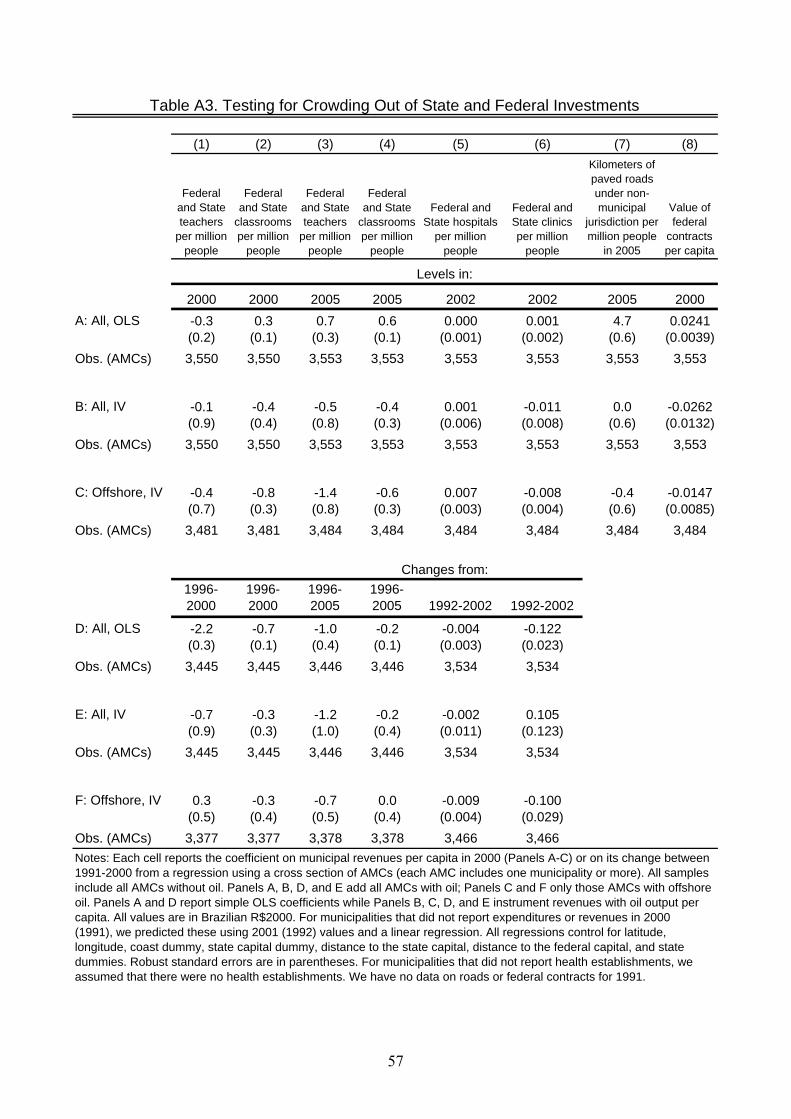
(1) (2) (3) (4) (5) (6) (7) (8)

Federal and State teachers

per million people

Federal and State

classrooms per million

people

Federal and State teachers

per million people

Federal and State

classrooms per million

people

Federal and State hospitals

per million people

Federal and State clinics per million

people

Kilometers of paved roads under non-municipal

jurisdiction per million people

in 2005

Value of federal

contracts per capita

2000 2000 2005 2005 2002 2002 2005 2000A: All, OLS -0.3 0.3 0.7 0.6 0.000 0.001 4.7 0.0241

(0.2) (0.1) (0.3) (0.1) (0.001) (0.002) (0.6) (0.0039)Obs. (AMCs) 3,550 3,550 3,553 3,553 3,553 3,553 3,553 3,553

B: All, IV -0.1 -0.4 -0.5 -0.4 0.001 -0.011 0.0 -0.0262(0.9) (0.4) (0.8) (0.3) (0.006) (0.008) (0.6) (0.0132)

Obs. (AMCs) 3,550 3,550 3,553 3,553 3,553 3,553 3,553 3,553

C: Offshore, IV -0.4 -0.8 -1.4 -0.6 0.007 -0.008 -0.4 -0.0147(0.7) (0.3) (0.8) (0.3) (0.003) (0.004) (0.6) (0.0085)

Obs. (AMCs) 3,481 3,481 3,484 3,484 3,484 3,484 3,484 3,484

1996-2000

1996-2000

1996-2005

1996-2005 1992-2002 1992-2002

D: All, OLS -2.2 -0.7 -1.0 -0.2 -0.004 -0.122(0.3) (0.1) (0.4) (0.1) (0.003) (0.023)

Obs. (AMCs) 3,445 3,445 3,446 3,446 3,534 3,534

E: All, IV -0.7 -0.3 -1.2 -0.2 -0.002 0.105(0.9) (0.3) (1.0) (0.4) (0.011) (0.123)

Obs. (AMCs) 3,445 3,445 3,446 3,446 3,534 3,534

F: Offshore, IV 0.3 -0.3 -0.7 0.0 -0.009 -0.100(0.5) (0.4) (0.5) (0.4) (0.004) (0.029)

Obs. (AMCs) 3,377 3,377 3,378 3,378 3,466 3,466Notes: Each cell reports the coefficient on municipal revenues per capita in 2000 (Panels A-C) or on its change between 1991-2000 from a regression using a cross section of AMCs (each AMC includes one municipality or more). All samples include all AMCs without oil. Panels A, B, D, and E add all AMCs with oil; Panels C and F only those AMCs with offshore oil. Panels A and D report simple OLS coefficients while Panels B, C, D, and E instrument revenues with oil output per capita. All values are in Brazilian R$2000. For municipalities that did not report expenditures or revenues in 2000 (1991), we predicted these using 2001 (1992) values and a linear regression. All regressions control for latitude, longitude, coast dummy, state capital dummy, distance to the state capital, distance to the federal capital, and state dummies. Robust standard errors are in parentheses. For municipalities that did not report health establishments, we assumed that there were no health establishments. We have no data on roads or federal contracts for 1991.

Table A3. Testing for Crowding Out of State and Federal Investments

Levels in:

Changes from:

57

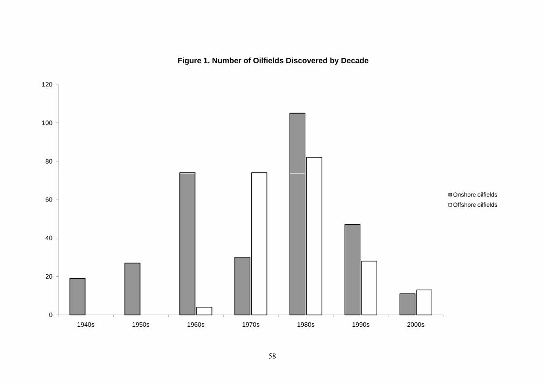
80

100

120

Figure 1. Number of Oilfields Discovered by Decade

0

20

40

60

1940s 1950s 1960s 1970s 1980s 1990s 2000s

Onshore oilfields

Offshore oilfields

58

Figure 2 AMCs (from 1970) and Oilfields in BrazilFigure 2. AMCs (from 1970) and Oilfields in Brazil

59

CENTRE FOR ECONOMIC PERFORMANCE Recent Discussion Papers

959 Iga Magda David Marsden Simone Moriconi

Collective Agreements, Wages and Restructuring in Transition

958 Carlos Daniel Santos Recovering the Sunk Costs of R&D: the Moulds Industry Case

957 Nicholas Oulton Ana Rincon-Aznar

Rates of Return and Alternative Measures of Capital Input: 14 Countries and 10 Branches, 1971-2005

956 Tim Leunig Chris Minns Patrick Wallis

Networks in the Premodern Economy: the Market for London Apprenticeships, 1600-1749

955 Urban Sila Can Family-Support Policies Help Explain Differences in Working Hours Across Countries?

954 John T. Addison Alex Bryson Paulino Teixeira André Pahnke Lutz Bellman

The Extent of Collective Bargaining and Workplace Representation: Transitions between States and their Determinants. A Comparative Analysis of Germany and Great Britain

953 Alex Bryson Harald Dale-Olsen Erling Barth

How Does Innovation Affect Worker Well-being?

952 Nathan Foley-Fisher Bernardo Guimaraes

US Real Interest Rates and Default Risk in Emerging Economies

951 Yann Algan Christian Dustmann Albrecht Glitz Alan Manning

The Economic Situation of First- and Second-Generation Immigrants in France, Germany and the United Kingdom

950 Jérôme Adda Francesca Cornaglia

The Effect of Bans and Taxes on Passive Smoking

949 Nicholas Oulton How to Measure Living Standards and Productivity

948 Alex Bryson Bernd Frick Rob Simmons

The Returns to Scarce Talent: Footedness and Player Remuneration in European Soccer

947 Jonathan Wadsworth Did the National Minimum Wage Affect UK Wages?

946 David Marsden The Paradox of Performance Related Pay Systems: ‘Why Do We Keep Adopting Them in the Face of Evidence that they Fail to Motivate?’

945 David Marsden Almudena Cañibano

Participation in Organisations: Economic Approaches

944 Andreas Georgiadis Alan Manning

One Nation Under a Groove? Identity and Multiculturalism in Britain

943 Andreas Georgiadis Alan Manning

Theory of Values

942 Kristian Behrens Giordano Mion Yasusada Murata Jens Südekum

Trade, Wages and Productivity

941 David Marsden Richard Belfield

Institutions and the Management of Human Resources: Incentive Pay Systems in France and Great Britain

940 Elhanan Helpman Oleg Itskhoki Stephen Redding

Inequality and Unemployment in a Global Economy

939 Norman Ireland Robin A. Naylor Jeremy Smith Shqiponja Telhaj

Educational Returns, Ability Composition and Cohort Effects: Theory and Evidence for Cohorts of Early-Career UK Graduates

938 Guy Mayraz Jürgen Schupp Gert Wagner

Life Satisfaction and Relative Income: Perceptions and Evidence

937 Nicholas Bloom Raffaella Sadun John Van Reenen

The Organization of Firms Across Countries

936 Jean-Baptiste Michau Unemployment Insurance and Cultural Transmission: Theory and Application to European Unemployment

935 João M. C. Santos-Silva Silvana Tenreyro

Trading Partners and Trading Volumes: Implementing the Helpman-Melitz-Rubinstein Model Empirically

934 Christian Morrisson Fabrice Murtin

The Century of Education

The Centre for Economic Performance Publications Unit

Tel 020 7955 7284 Fax 020 7955 7595 Email info@cep.lse.ac.uk Web site http://cep.lse.ac.uk