Loughborough UniversityInstitutional Repository

Boundary-layer analysis ofthe thermal bar

This item was submitted to Loughborough University's Institutional Repositoryby the/an author.

Citation: KAY, A., KUIKEN, H.K. and MERKIN, J.H., 1995. Boundary-layer analysis of the thermal bar. Journal of Fluid Mechanics Digital Archive,303, pp. 253-278

Additional Information:

• This article was published in the Journal of Fluid Mechan-ics [ c© Cambridge University Press] and is also available at:http://journals.cambridge.org/action/displayAbstract?aid=340146

Metadata Record: https://dspace.lboro.ac.uk/2134/4236

Version: Published

Publisher: c© Cambridge University Press

Please cite the published version.

This item was submitted to Loughborough’s Institutional Repository (https://dspace.lboro.ac.uk/) by the author and is made available under the

following Creative Commons Licence conditions.

For the full text of this licence, please go to: http://creativecommons.org/licenses/by-nc-nd/2.5/

.I. Fluid Mech. (1995), 001. 303, pp. 253-278 Copyright 0 1995 Cambridge University Press

253

Boundary-layer analysis of the thermal bar

By A N T H O N Y KAY', H. K. K U I K E N 2 AND J. H. MERKIN2 'Loughborough University of Technology, Loughborough, Leicestershire, LEI 1 3TU, UK

'University of Leeds, Leeds, LS2 9JT, UK

(Received 6 September 1994 and in revised form 13 July 1995)

The thermal bar, a descending plane plume of fluid at the temperature of maximum density (3.98"C in water), is analysed as a laminar free-convection boundary layer, following the example of Kuiken & Rotem (1971) for the plume above a line source of heat. Numerical integration of the similarity form of the boundary-layer equations yields values of the vertical velocity and temperature gradient on the centre line and the horizontal velocity induced outside the thermal bar as functions of Prandtl number 0. The asymptotic behaviour of these parameters for both large and small 0 is also obtained; in these cases, the thermal bar has a two-layer structure, and the method of matched asymptotic expansions is used. For the intermediate case 0 = 1, an analytical calculation using approximate velocity and temperature profiles in the integrated boundary-layer equations yields good agreement with the numerical results. The applicability of the results to naturally occurring thermal bars (e.g. in lakes) is limited, but the laminar-flow analysis is likely to relate more closely to the phenomenon on a laboratory scale.

1. Introduction Water and several metals have their maximum density in the liquid phase, p,, at

a temperature T, above the melting temperature; for water at sea-level atmospheric pressure, T, = 3.98"C. Suppose there is a monotonic variation of temperature T with horizontal coordinate y in a body of such a liquid, with T = T, at y = 0. The density p has a maximum with respect to y and the sign of ap/dy changes at y = 0. Thus, on opposite sides of the plane y = 0, the baroclinicity

1 -(gradp x gradp) P2

and the resultant vorticity production will have opposite directions. A double-cell circulation will therefore be produced (figure l), with the densest water sinking on the plane y = 0.

The horizontal convergence in the upper half of the flow will steepen the tempera- ture gradient there. Even with an initially linear temperature variation, as suggested in figure 1, the isotherm pattern will eventually take on the form shown in figure 2, with a sharp front at y = 0. When heat conduction balances convection, the isotherm pattern can become steady. Such a front was first observed by Fore1 (1880) in Lake Geneva; he designated it barre thermique since it formed a barrier between bodies of water cooler and warmer than 4°C. The presence of such a thermal bar in a lake is of practical importance in that pollutants discharged on one side of the bar cannot pass

254 A. Kay, H . K . Kuiken and J . H . Merkin

T

FIGURE 1. Baroclinic circulation created by a linear horizontal temperature variation through the temperature of maximum density. (a) Temperature and density profiles, ( b ) streamlines.

FIGURE 2. Isotherm pattern resulting from the circulation in figure 1, showing frontal structure.

across it, thus reducing the volume of water available for their dilution (Hubbard & Spain 1973).

Lacustrine thermal bars commonly arise because warming (in Spring) or cooling (in Autumn) proceeds more rapidly in shallow than in deep water. Thus the isotherm T = T,,, first appears at the shore and then migrates towards deeper water, eventually disappearing when the entire lake is warmer or cooler than T,. Zilitinkevich, Kreiman & Terzhevik (1992) have reviewed the features of this form of thermal bar: it may be inclined to the vertical (Elliot 1971), and the temperature field is asymmetric, with stable stratification on the shoreward side but convective overturning, resulting in vertically well-mixed conditions, on the deep-water side. More recently, Farrow (1995~) has shown that in this unsteady flow the downwelling front (marked by the streamline descending from the surface stagnation point) may become separated from the thermal front (marked by the isotherm T = T,). All the above authors ignored Coriolis effects; however, those researchers concerned with the North American Great Lakes have identified the dominant flow to be the ‘thermal wind’, a horizontal flow parallel to the thermal bar deriving from a balance between buoyancy and Coriolis

Boundary-layer analysis of the thermal bar 255

forces (Brooks & Lick 1972; Huang 1972). A circulation similar to that in figure 1 will still exist in planes normal to this thermal wind.

While the mathematical models of the above-mentioned authors have all yielded useful information about the circulation in a lake containing a thermal bar, none has investigated the flow and temperature field within a thermal bar in detail. However, as early as 1902 Witte had described the curtain of descending water of maximum density as a boundary layer (grenzschicht). Garrett & Horne (1978) pointed out the similarity between the thermal bar and the free-convection boundary layer on an isothermal plate immersed in a cooler fluid. The latter problem was solved by Ostrach (1953); Garrett & Horne, being interested only in the order of magnitude of the vertical flow, applied Ostrach’s result to the thermal bar but added that the absence of a no-slip boundary would allow a greater flow speed. The object of the present paper is to use the boundary-layer analogy to analyse precisely the flow in a thermal bar.

The boundary-layer analysis will require the following assumptions : zero heat flux through the free surface; symmetry about the isotherm T = T,; steady flow, with a stationary, vertical thermal bar. These assumptions are at variance with the features described above for thermal bars arising during Spring warming and Autumn cooling of lakes; nevertheless, Farrow’s (199%) numerical model of the Spring thermal bar indicates that when inertia is dominant a boundary-layer structure, albeit highly asymmetric, does appear. The asymmetry will be less marked in a thermal bar which is migrating less rapidly, as may be the case at the confluence of two bodies of water with temperatures on either side of T,; such phenomena have been studied by Carmack (1979) at the inflow of a river into a lake. There remains the criticism that naturally occurring thermal bars are turbulent, whereas the boundary-layer analysis assumes laminar flow. The parametrization of turbulent mixing by eddy diffusivities (of heat and momentum), which leaves the equations in the same form, may have some justification when considering the large-scale circulation in a lake but is inappropriate for a detailed study of the thermal bar. However, laminar-flow analysis should be relevant to laboratory experiments on thermal bars, such as those of Ivey & Hamblin (1989, hereafter referred to as IH). The issue of laminar us. turbulent flow is discussed in more detail in $5 below.

2. Governing equations and boundary conditions We are concerned only with the flow within the thermal bar, which has a lateral

length scale which is small compared to the geometrical scales of any lake or laboratory tank. We therefore ignore side boundaries and any external heat fluxes which may be ultimately responsible for creating the thermal bar. The self-similarity which will be used in the boundary-layer analysis also requires that we assume the body of fluid to have infinite depth. In a container of finite depth, a thermal bar can exist only as a sharp front where the horizontal flow is convergent, i.e. in the upper half of the container; our analysis may be expected to apply fairly accurately in this region. IH refer to there being no clearly defined front beyond 70% of the depth of their laboratory tank, although in some experiments they observed the descending flow to become unstable at a critical depth, where it suddenly started to meander horizontally.

We consider steady two-dimensional flow in the half-plane x > 0, where the coordinate x is measured vertically downwards. The flow and heat transfer are described by boundary-layer equations, in which vertical diffusion of momentum and

256 A. Kay, H. K . Kuiken and J. H . Merkin

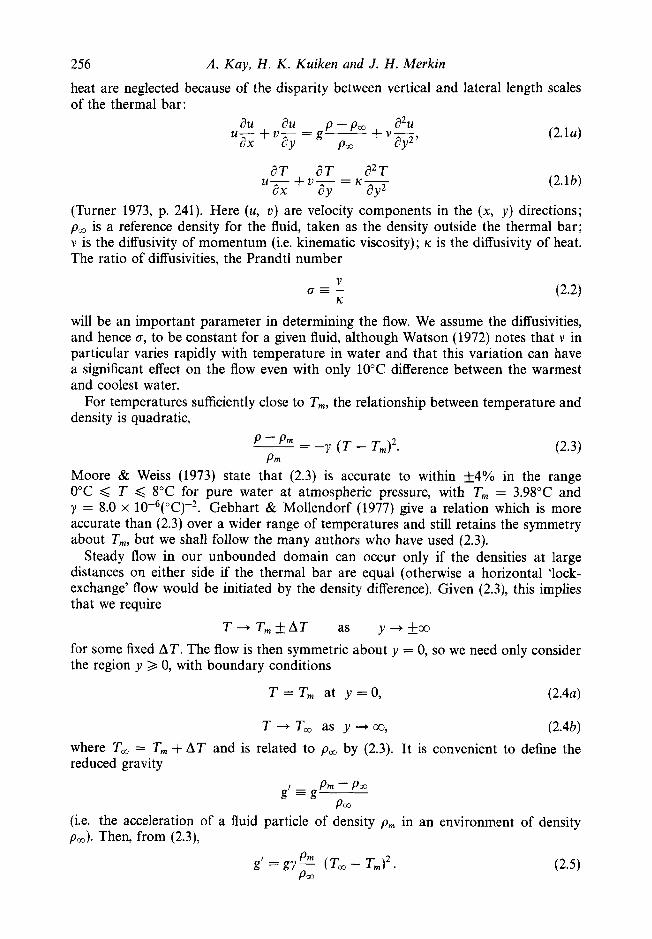
heat are neglected because of the disparity between vertical and lateral length scales of the thermal bar:

au au p - p , a2U u- + u- = g - + V - - - ,

ax a y Pw a y

aT aT a2T u- +u- = Ic-

ax a y ay2

(2.lu)

(2.lb)

(Turner 1973, p. 241). Here (u, u ) are velocity components in the (x, y) directions; pa, is a reference density for the fluid, taken as the density outside the thermal bar; v is the diffusivity of momentum (i.e. kinematic viscosity); IC is the diffusivity of heat. The ratio of diffusivities, the Prandtl number

will be an important parameter in determining the flow. We assume the diffusivities, and hence CT, to be constant for a given fluid, although Watson (1972) notes that v in particular varies rapidly with temperature in water and that this variation can have a significant effect on the flow even with only 10°C difference between the warmest and coolest water.

For temperatures sufficiently close to T,, the relationship between temperature and density is quadratic,

(2.3) -- - P m - -y ( T - T,,J2. P m

Moore & Weiss (1973) state that (2.3) is accurate to within &4% in the range 0°C ,< T ,< 8°C for pure water at atmospheric pressure, with T, = 3.98”C and y = 8.0 x 10-6(oC)-2. Gebhart & Mollendorf (1977) give a relation which is more accurate than (2.3) over a wider range of temperatures and still retains the symmetry about T,, but we shall follow the many authors who have used (2.3).

Steady flow in our unbounded domain can occur only if the densities at large distances on either side if the thermal bar are equal (otherwise a horizontal ‘lock- exchange’ flow would be initiated by the density difference). Given (2.3), this implies that we require

T+T,+AT as y+&00

for some fixed AT. The flow is then symmetric about y = 0, so we need only consider the region y 2 0, with boundary conditions

T = Tm at y = 0, (2.4~)

T -+ T, as y + 00, (2.4b) where T, = T,,, + AT and is related to p , by (2.3). It is convenient to define the reduced gravity

(i.e. the acceleration of a fluid particle of density pm in an environment of density p , ) . Then, from (2.3),

g’ = gy (T , - Tm)2. P a

(2.5)

Boundary-layer analysis of the thermal bar 257

Introducing the dimensionless temperature

T - T,

Tm - Tm e r

and using (2.3) and (2.6), the momentum and heat transfer equations (2.1) become

au au a 2 U U- + v - = g ' ( 2 8 - 0 ~ ) + ~ - ,

ax a y aY2

ae ae a20 u- + 0- = K-. ax ay a y 2

We also require the continuity equation, which takes the form

( 2 . 7 ~ )

(2.7b)

since density variations are too small for compressibility effects to be important. Boundary conditions on the flow at y = 0 are determined by the requirements of

symmetry. Far from the thermal bar there is no vertical motion. Thus the complete set of boundary conditions is

( 2 . 9 ~ )

u - 0 , 8 - 0 as y + m , (2.9b) where conditions (2.4) have been re-written in terms of 8. The self-similarity of the thermal bar implies conditions at the upper surface,

u = 0, 0 = 0 at x = 0 (for y > 0),

while the boundary-layer formulation eliminates any consideration of stress or heat flux at x = 0.

Gebhart et al. (1988) have reviewed theoretical investigations of free convection in water near its temperature of maximum density. There have been numerous studies of external flows induced by inserting a surface at a prescribed temperature or by applying a prescribed heat flux at a vertical plane; Gebhart & Mollendorf (1978) supply a comprehensive set of results on such flows. However, there appear to have been no investigations of the case where the only externally prescribed conditions are the temperatures at y = +_a (a problem which is well-posed only when there is a density maximum between those far-field temperatures).

Also of relevance are studies of flows in cavities with end-walls at temperatures either side of Tm. Lin & Nansteel's (1987) numerical calculations show a thermal bar structure at a Rayleigh number (Ra = g'd3/(vrc), where d is the depth of the cavity) of lo6. IH obtained a thermal bar in their experiments, but their asymptotic calculations followed in the tradition established by Cormack, Leal & Imberger (1974) of using the aspect ratio of the cavity, rather than the reciprocal of Rayleigh number, as the small parameter of primary importance. Thus their analysis does not resolve the thermal bar as a narrow boundary layer.

In the present paper the emphasis will be on analytical results, although comparison will be made with numerical solutions of the governing equations (obtained as described below). In particular, we shall be concerned with the dependence of flow speeds and heat transfer rates on Prandtl number 6. For water at 3.98"C, CT = 11.6, while liquid metals generally have values of CT of order Thus we shall obtain

at4 - = O , v=O, 8 = 1 at y = O , aY

258 A. Kay, H . K. Kuiken and J . H . Merkin

asymptotic solutions for both large and small (T, following the example of Kuiken & Rotem (1971) who investigated the laminar plume above a line source of heat.

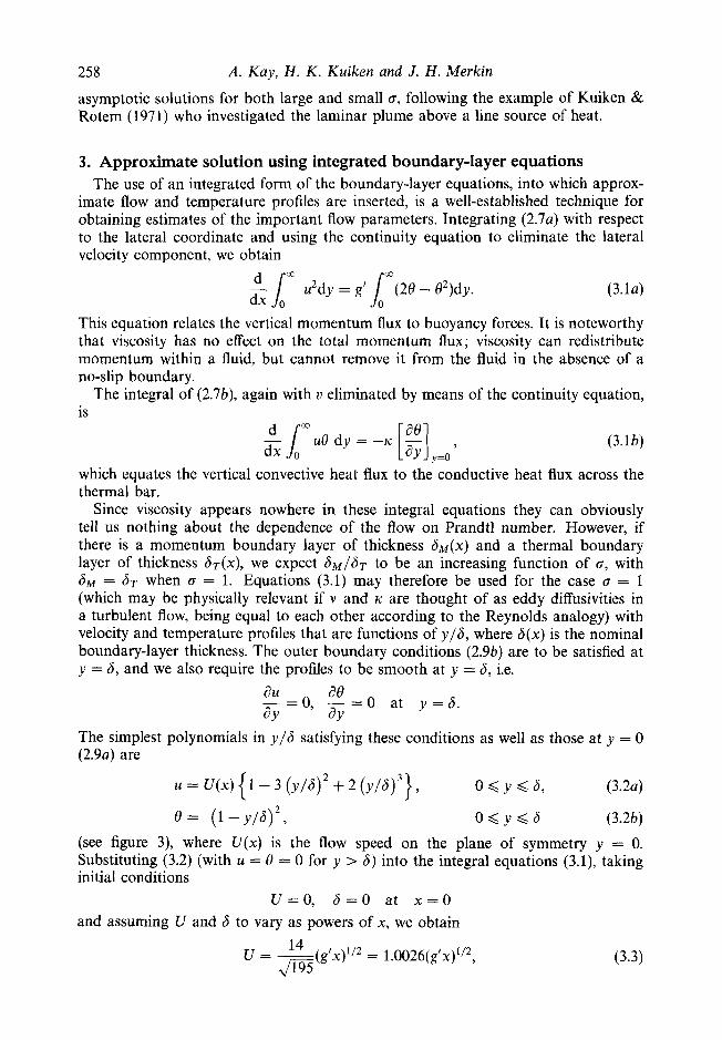
3. Approximate solution using integrated boundary-layer equations The use of an integrated form of the boundary-layer equations, into which approx-

imate flow and temperature profiles are inserted, is a well-established technique for obtaining estimates of the important flow parameters. Integrating ( 2 . 7 ~ ) with respect to the lateral coordinate and using the continuity equation to eliminate the lateral velocity component, we obtain

00

u2dy = g' 1 (20 - 02)dy. dx

( 3 . 1 ~ )

This equation relates the vertical momentum flux to buoyancy forces. It is noteworthy that viscosity has no effect on the total momentum flux; viscosity can redistribute momentum within a fluid, but cannot remove it from the fluid in the absence of a no-slip boundary.

The integral of (2.7b), again with u eliminated by means of the continuity equation, is "1 00 u 8 d y = - r [ g ] ,

dx y=o (3.lb)

which equates the vertical convective heat flux to the conductive heat flux across the thermal bar.

Since viscosity appears nowhere in these integral equations they can obviously tell us nothing about the dependence of the flow on Prandtl number. However, if there is a momentum boundary layer of thickness 6M(x) and a thermal boundary layer of thickness 6T(x), we expect 6w/6T to be an increasing function of (T, with 6~ = 6~ when (T = 1. Equations (3.1) may therefore be used for the case (T = 1 (which may be physically relevant if v and IC are thought of as eddy diffusivities in a turbulent flow, being equal to each other according to the Reynolds analogy) with velocity and temperature profiles that are functions of y/6, where 6(x) is the nominal boundary-layer thickness. The outer boundary conditions (2.9b) are to be satisfied at y = 6, and we also require the profiles to be smooth at y = 6, i.e.

au ae a Y dY - = O , - = 0 at y = 6 ,

The simplest polynomials in y/6 satisfying these conditions as well as those at y = 0 (2 .9~) are

(3 .2~)

(3.2b)

(see figure 3), where U ( x ) is the flow speed on the plane of symmetry y = 0. Substituting (3.2) (with u = 0 = 0 for y > 6) into the integral equations (3.1), taking initial conditions

U = O , 6 = 0 at x = O and assuming U and 6 to vary as powers of x, we obtain

2 8 = (1-Y/6) , O d Y < 6

14 U = ---(g'x)1/2 = 1.0026(g'~)'/~, Jm (3.3)

Boundary-layer analysis of the thermal bar

f’

I I I I I I

0 2 4 6 0 2 4 6

259

FIGURE 3. Profiles of (a) dimensionless vertical velocity u/(g’x)1’2 and ( b ) dimensionless temperature 8, for c = 1. The abscissa is the similarity variable q , defined in (4.2). Solid lines: numerical solution. Dashed Iines: approximate profiles (3 .2) , scaled according to results (3.3), (3.4).

The result (3.3) compares well with that obtained from numerical integration of the exact boundary-layer equations for (T = 1, namely

U = 0.9833 (g’x)’/2. (3.5)

It is also of interest to compare these results with previous estimates of vertical flow speeds in thermal bars. Witte (1902) used

the fall speed of a heavy body sinking in an inviscid fluid. In the light of (3.la), he may be considered as justified in his inviscid assumption, but he neglected the need for buoyancy forces to provide for horizontal transport of vertical momentum (the term vdu/dy in ( 2 . 7 ~ ) ) in order to satisfy continuity: hence he overestimated U . In contrast, Garrett & Horne (1978) used

U = 0 . 5 ( g ’ ~ ) ’ / ~ ,

260 A. Kay, H. K. Kuiken and J. H . Merkin

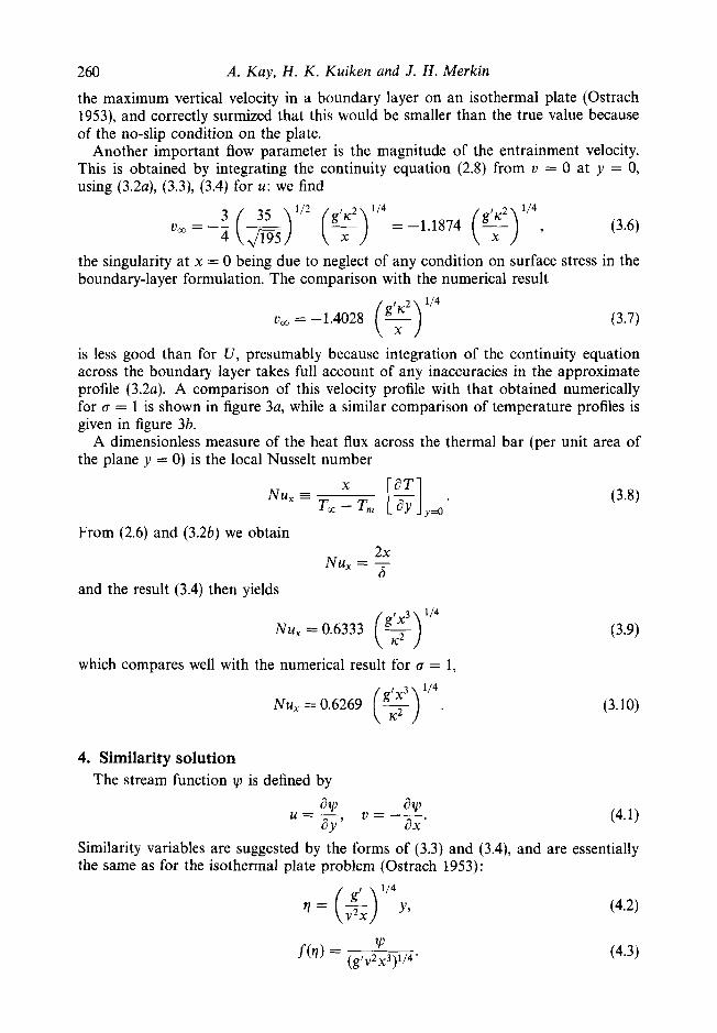
the maximum vertical velocity in a boundary layer on an isothermal plate (Ostrach 1953), and correctly surmized that this would be smaller than the true value because of the no-slip condition on the plate.

Another important flow parameter is the magnitude of the entrainment velocity. This is obtained by integrating the continuity equation (2.8) from v = 0 at y = 0, using (3.2a), (3.3), (3.4) for u : we find

the singularity at x = 0 being due to neglect of any condition on surface stress in the boundary-layer formulation. The comparison with the numerical result

114

v, = -1.4028 (q) (3.7)

is less good than for U , presumably because integration of the continuity equation across the boundary layer takes full account of any inaccuracies in the approximate profile (3.2~). A comparison of this velocity profile with that obtained numerically for CT = 1 is shown in figure 3a, while a similar comparison of temperature profiles is given in figure 3b.

A dimensionless measure of the heat flux across the thermal bar (per unit area of the plane y = 0) is the local Nusselt number

From (2.6) and (3.2b) we obtain 2x

N U , = - 6

and the result (3.4) then yields

114

Nu, = 0.6333 (G) which compares well with the numerical result for CT = 1,

1 I4 Nu, = 0.6269 (5)

4. Similarity solution The stream function y is defined by

(3-9)

(3.10)

Similarity variables are suggested by the forms of (3.3) and (3.4), and are essentially the same as for the isothermal plate problem (Ostrach 1953):

Boundary-layer analysis of the thermal bar 26 1

(The use of v instead of K which appears in (3.4) is conventional, and simply causes the Prandtl number to appear in a different position in the subsequent equations.) The velocity components are then

u = (g’x)1/2f’(q), ( 4 . 4 ~ )

(4.4b)

and the momentum and heat transfer equations (2.7) become

f”’ + iff’’ - 4j-Q + 26 - 0 2 = 0,

e” + Safe’ = o

( 4 . 5 ~ )

(4.5b) (where primes denote differentiation with respect to q) . The boundary conditions (2.9) become

f = 0, f ” = 0, 6 = 1 at q = 0, ( 4 . 6 ~ )

f ’ - + O , 8 - 0 as q + c o . (4.6b) Equations ( 4 3 , (4.6) were solved numerically using a standard two-point boundary- value solver in the NAG library. Converged solutions of high accuracy were readily obtained using this procedure for a wide range of values of a (from O( lo-*) to O( lo2)). The only problem encountered was in obtaining solutions for very small values of (T,

where care had to be exercised to ensure that the outer boundary conditions were applied at a sufficiently large value of q to retain accuracy.

As in $3 above we shall be interested in the vertical flow speed at the plane of symmetry, the lateral flow speed outside the thermal bar and the Nusselt number for heat transfer across the thermal bar. These quantities are related to f(q) and 6(q) by

u = (g’X)’/2f’(o), (4.7)

(4.9)

Although it is physically relevant to obtain results only at those values of Prandtl number which apply at temperature T,,, for those few liquids having maximum density above the melting temperature, we have obtained f’(O), f(m) and e’(0) as functions of a for the full range of a.

We have also obtained asymptotic results valid for large and small values of a ; details of the analysis are given in Appendices A and B respectively. For large (T we find that

f‘(0) - a-1/4 (1.30051 - 0.664760-’/~ + . . .) (4 .10~)

eqo) - -03/8 (0.78800 - 0.267600-’/~ + . . .) (4.10b)

f ( c o ) - (1.36987 - 0.091820-’/~ + . . .) as (T -+ 00. (4.10~)

These asymptotic results are plotted together with those obtained numerically for a 2 1 in figure 4; the abscissa is a logarithmic axis for a (to give due emphasis to very large values of a, for which the asymptotic results should be most accurate), and

as a -+ co,

as a -+ 03,

262

cr1/4 ~ ( 0 ) 0.9 -

0.7 -

-

0.5

A.

1’3 1.1 1 ,,’-

,,/ I I I

I I I I I I I I I I ,

,,,‘ I

-.,

I I 1 I I I I I I

Kay, H. K. Kuiken and J . H. Merkin

(b) I I

0.6 -

-

0.5

I I , I I I I , I I I

,,**’

I I I I I I I I I

I I

FIGURE 4. Results from numerical integration of (4.5) (solid lines) and asymptotic formulae (4.10) (dashed lines) for 0 1. The broken vertical line is at Q = 11.6, corresponding to water at 3.98”C. (a) Dimensionless vertical velocity on plane of symmetry, scaled as c~’/~f’(O). ( b ) Dimensionless temperature gradient on plane of symmetry, scaled as 0-3/sO’(0). (c) Dimensionless far-field horizontal velocity, scaled as oilsf(.o).

Boundary-layer analysis of the thermal bar 263

the ordinates are c~’/~f’(O), -G-~ / ’O’ (O) and o’/’f(co), since the behaviour as a -+ co is shown most clearly when the dependent variable approaches a non-zero constant in this limit. There is good agreement between asymptotic and numerical results for a as low as unity in the case of the heat transfer parameter O’(0). The asymptotic results for the flow-speed parameters are less accurate at moderate values of a; however the only value of a(> 1) of practical importance in laminar flow is a = 11.6 (i.e. for water at its temperature of maximum density), at which the errors are 5.6% for f’(O), 2.6% for O’(0) and 7.0% for f(co).

For small a we find that

f’(0) - 1.4142 - 1 . 1 5 6 0 ~ ~ ’ ~ + 0.85900 + . . . , (4.11~)

eqo) - -01/2(o.6554 - 0.03968~ + . . .), (4.11b)

f(m) - 1.5861 + 0.27020 + . . .). (4.11~)

We plot the quantities f’(O), -o-’/%’(O) and a’/*f(co) for a d 1 in figure 5, comparing the asymptotic results (4.11) to those obtained by numerical integration of (4.5); as well as ensuring that the dependent variables approach non-zero constants as a -+ 0, the rescaling of O’(0) and f(m) is natural for the case where K > v , in the sense that

114 3 g’K2 = 4 ( y-) (a1/2f(co)) .

Agreement between the asymptotic and numerical results is good, especially in the case of ~ ‘ / ~ f ( c o ) for which the error in (4.11~) remains small even for a = 1.

5. Discussion The flow and heat transfer in a laminar thermal bar have been analysed by the

classical methods of boundary-layer theory. This is possible because the convergence of the horizontal flow ensures that the lateral length scale of a thermal bar is small compared to its vertical extent. The similarity equations have been solved numerically for all values of Prandtl number a and also, as in Kuiken & Rotem’s (1971) study of the rather similar problem of a laminar plume above a line source of heat, by matched asymptotic expansions for both large and small a. The asymptotic calculations do involve some numerical integration, but provide more insight into the dependence of the flow on Prandtl number than is obtained by a purely numerical solution.

The thermal bar has a two-layer structure, with the ratio between the momentum and thermal layer thickness scaling as

For 091, viscosity is a leading-order constraint on the flow; at the same time, any increase in heat diffusion would result in the production of a greater quantity of fluid denser than pm, and so greater buoyancy forces to drive the flow. Hence, for fixed v ,

264

-

0.61

A. Kay, H . K . Kuiken and J . H. Merkin

'. .. -.-..

I I I I I I I I I I

1.5 1 , ,

0.9 I I I I I I I I I I

0 0.2 0.4 0.6 0.8 1.0

I I I I I I I I I I I

0 0.2 0.4 0.6 0.8 1 .o

FIGURE 5. Results from numerical integration of (4.5) (solid lines) and asymptotic formulae (4.11) (dashed lines) for Q < 1. (a) Dimensionless vertical velocity on plane of symmetry, f '(0). (b) Dimensionless temperature gradient on plane of symmetry, o-1/20'(0). (c) Dimensionless far-field horizontal velocity, o ' / ~ ~ ( c D ) .

0

265 Boundary-layer analysis of the thermal bar

the flow speeds increase with K according to

u cc U1l4 , u, K K1I8

at leading order (see (4.10)). Greater convection of momentum inwards and downwards (while the outward

diffusion of momentum remains constant) implies that the momentum boundary layer becomes thinner: thus 8~ is indirectly influenced by heat conduction, with (A33) indicating that

8 M a K - ’ / ~ .

The greater thickness of the thermal boundary layer with increased heat conduction,

BT K

results in a reduced temperature gradient and hence reduced Nusselt number,

Nu, K K - ~ / ~

(from (4.10b)); however, the heat flux across the thermal bar, being proportional to K N u ~ , does of course increase with ic.

The scalings are simpler in the case gel, where viscosity merely produces a fine adjustment to a flow controlled by buoyancy and heat conduction. To leading order the parameters U , om and Nu, are all independent of v ; indeed the Nusselt number varies very little over the entire range 0 < CT < 1, as the temperature profile is almost unaffected by the viscous inner layer.

The free descending plume at the thermal bar may be compared with a wall plume at a vertical wall held at the temperature T,. Gebhart & Mollendorf (1978) gave results for the latter, although they used a different equation of state for water which is more accurate than (2.3) at temperatures not close to T,. They did not undertake any asymptotic analysis comparable to ours, so we restrict our comparison to the numerical results at 0 = 11.6. It is found that the no-slip condition at a wall reduces the vertical mass flux by 17% and the heat flux by 39% compared to that in a thermal bar with a zero-stress condition on the plane of symmetry. The retardation of the flow near a wall has a relatively small effect on the total mass flux; however, with CT > 1 the thermal boundary layer is thin compared to the viscous layer, so most of the convective heat transfer is occurring within the near-wall region where the velocity difference between the wall plume and the thermal bar is greatest. This explains the greater effect of the wall on heat transfer than on mass flux.

Boundary-layer analysis breaks down in some region close to the ‘leading edge’ x = 0 (in this case the liquid surface). For CT > 1, the outer-layer thickness is

the layer can only be considered thin where BMex, i.e. for x+xg where

113

xg = CT1I6 ($) .

In water with T, - T, = 1°C (a typical value found in lacustrine thermal bars), xg FS 5 mm, which suggests that the analysis should be valid even in most laboratory tanks, especially since xg cc (T , - TJ2l3 and many experiments have involved larger values of the temperature difference than 1°C.

266 A. Kay, H. K . Kuiken and J. H . Merkin

At greater depths, a thermal bar may become turbulent. Using a criterion originally obtained for BCnard convection, Zilitinkevich et al. (1992) suggest that transition to turbulence should occur at a depth of a few centimetres. However, it is possibly more appropriate to compare the thermal bar with a plane plume, for which Gebhart et al. (1988, $11.8) indicate that transition is complete when

~ r , = 3 x 107 (5.2)

where the local Grashof number is defined as

g’x3 Gr, = --.

V2 (5.3)

This indicates that a thermal bar in water with T, - T, = 1°C will be turbulent at depths greater than about 1 m. The criterion (5.2) yields a later transition to turbulence than was found by IH, who observed the descending flow to become unstable for Gr 2 lo6; however, it is not clear to what extent this was influenced by the divergence of the horizontal flow below mid-depth in their rather shallow experimental tank, as opposed to being purely an instability to random disturbances.

A fully turbulent thermal bar may reach the stage where the transport of momentum and heat becomes independent of the molecular properties of the liquid (v and ic), and the lateral growth of the thermal bar is due entirely to entrainment of fluid from either side by the self-generated turbulence of the descending flow. In this case, a simple model of the flow is provided by the assumption of an entrainment velocity ve proportional to the vertical velocity (Morton, Taylor & Turner 1956), implying that the width S of the thermal bar must increase linearly with depth, in contrast to the case of the laminar plume for which 6 cc x1/4. On the other hand, since the flow is controlled by the buoyancy g’ (rather than a buoyancy flux as in Morton et al.’s plumes), the vertical velocity must still scale as (g’x)1/2. Suppose the profiles of vertical velocity and density across the thermal bar are

(5.4a)

(5.4b)

where the functions 41, q2 are likely to be approximately Gaussian (Turner 1973) and the temperature profile is obtainable from (5.4b) by (2.3): defining the entrainment constant CI by

u, = au, we then obtain from mass and momentum balances that

1/2

u = (&) (g’x)”2,

2

Boundary-layer analysis of the thermal bar 267

While this analysis relates to self-generated turbulence, it is likely that in a geo- physical context there may be ambient turbulence providing transport of heat and momentum at much greater rates than molecular diffusion. Modellers such as Huang (1972) and Brooks & Lick (1972) have used eddy diffusivities typically 3 orders of magnitude greater than the kinematic viscosity of water. An eddy diffusion model would of course leave the form of the governing equations unchanged from the case of laminar flow, although the thermal bar would be broader and so the boundary-layer formulation would become valid only at a greater depth. A more serious objection is that, while the parametrization of the effects of turbulence by eddy diffusivities may be appropriate when considering the large-scale flow in a lake, it has no justification when modelling a region which may be narrower than the length scale of the largest eddies; nevertheless, Garrett & Horne (1978) did use eddy diffusivities in estimating thermal bar parameters, while expressing uncertainty about the appropriate values to take in a lake.

Even if there is little or no turbulent mixing within the bulk of a lake, any wind across its surface may induce mixing in a surface layer. This is particularly relevant in the case of a thermal bar, which is assumed in the boundary-layer analysis to have zero thickness at the surface. This initial condition would not hold if wind-induced mixing created a transition region of non-zero width in which the surface temperature varied gradually from T,,, - AT to T,,, + AT, and the assumption of self-similarity would be invalid.

Another feature which is not addressed in our analysis is the asymmetry in tem- peratures about T,,, which typically occurs in a thermal bar at the confluence of two bodies of water (Carmack 1979). The laboratory experiments of Marmoush, Smith & Hamblin (1984) are relevant here: a barrier was removed between two bodies of water at initially uniform temperatures either side of T,. If there had been symmetry about T,,,, a steady thermal bar would have ensued and the experiment would have been the best realization possible in the laboratory of the theoretical model we have studied. With asymmetric temperatures, steady flow is not possible; instead, there is a lock-exchange flow, with oppositely directed gravity currents of denser water along the base of the tank and lighter water near the surface. There is vigorous mixing at the head of such gravity currents (Simpson 1987), and the mixed water is at temperatures closer to T,,, than either of the original bodies of water; it is therefore denser, and may form a steady sinking plume (as observed by Marmoush et al. 1984) once the gravity currents have been brought to rest. To fully understand this thermal bar would require the solution of the initial-value problem describing the unsteady flow leading to its formation. Similarly, the observations of Carmack (1979) that a river flowing into a lake can form a symmetric thermal bar with further regions of temperature change at some distance away (to take up the asymmetry about T,,,) would need to be understood by analysing the unsteady flow, starting from some initial condition before the thermal bar had appeared.

Appendix A. Asymptotic solution at large Prandtl number The limit 0 + co (i.e. K + 0) is singular: if K = 0 the temperature field, and hence

the flow, could not be in equilibrium, but for finite arbitrarily large 0 equilibrium is possible with a double-layer structure (Kuiken & Rotem 1971). In this case heat is diffusing much more slowly than momentum. Thus the temperature will differ significantly from T, only in a narrow inner layer; buoyancy forces will accelerate the fluid downwards in this layer, but the momentum will then diffuse outwards to a

268 A. Kay, H. K. Kuiken and J . H. Merkin

much broader outer layer. There is no buoyancy in the outer layer, and the flow here will be determined by a balance between viscous forces and inertia.

The disparity between the layer thicknesses suggests that the vertical velocity will, to a first approximation, be uniform across the inner layer. From (4.4a) and the boundary condition (4.6a), this implies

f bo(a)'1 (A 1)

in the inner layer, where the function bo(a) is yet to be determined. Substituting (Al) into ( 4 3 ) and using the boundary conditions on 0 in (4.6) yields

Anticipating that bo(o) has the form

bo(a) = Boaa

where Bo and 01 are constants, (A2) becomes

where

is the rescaled independent variable for the inner layer.

p = '10 (a+l)/2

A rescaling is also required for the outer layer:

c 3 aBy, F = a-B f .

This transforms (4.5a) to

dc3 4 dc2 d3F 3 d2F - + - F - - + ap48H(p) = 0

where

with 0 given by (A4), so that in the outer layer where 0 = 0 the rescaling (A6) leaves the form of (4.5a) unchanged. Integrating (A7) with respect to 5 and noting that

2 ~ ( p ) = 28 - e

p = 5@@+1-28)/2

we obtain

For fixed small ( as a + m, the last term in (A8) represents the overall effect of buoyancy forces in the inner layer on the flow in the outer layer, and so must remain finite and non-zero; hence

To determine a further relation between a and p, we note that the solution for F in the outer layer must match with that for f in the inner layer. The latter is given by (Al) and (A3), and when transformed by (A6) yields

~ 1 + 1 + 6p = 0. (A9)

F - B o ~ T ~ - ~ ~ ~ for (91 (fw

Boundary-layer analysis of the thermal bar 269

which again must be finite and non-zero for fixed small [ as CJ -+ co. Thus

a - 2p = 0,

which, together with (A9), gives

In the inner layer the independent variable is thus

3/8 p=CJ r l ; (A13a)

6 - O(1) and falls to zero while p N O(1), so the two terms in the thermal equation must be of the same order. This is ensured by letting

4 ( P ) = CJ5’V , e(p) = e. (A13b, c )

Equation (4.5) is thus transformed to

4’’’ + 0-1/2(20 - 6 2 ) + CJ-1(;4~” - &y2) = 0

e” + ;#Ie‘ = o where primes denote differentiation with respect to p. The boundary conditions are

(A14a)

(A14b)

4 = 0, #I” = 0, B = 1 on p = 0, (Al5a)

8 + 0 as p + m ; (A15b)

the outer boundary condition on #I will be determined by matching with the outer- layer solution.

Equation (A14a) suggests the expansion for large CJ,

(A16a)

e(p; 0) = eo(p) + d / 2 e 1 ( p ) + 0-le2(p) + . . . . (A16b)

At leading order, only the viscous term is present in the momentum equation (cf. Kuiken & Rotem 1971); the uniform-flow solution (Al), (A3), which transforms to

4 ( p ; CJ) = #Io(p) + 0-1/2#Il(p) + CJ-l#I2(p) + . . .,

#I0 = Bop, (‘417)

reflects this dominance of viscous forces. Equation (A4) is the leading-order solution for 0, i.e.

with Bo still to be determined. At 0 (cJ-’/~) there is a balance of buoyancy and viscous forces,

47 = e; - 2e0,

07 + i40e; = -f#Ile;;

(A191

(A201

(Pl(0) = 0, &(O) = 0, B,(O) = 0, 81(m) = 0. (A211

while the perturbation to the temperature is determined by

the boundary conditions are

270 A. Kay, H. K. Kuiken and J . H . Merkin

To eliminate the unknown Bo (in (A17), (A18)) from these equations, we rescale by

= ~ i / ~ 4 ~ , 0, = B&, p = B : / ~ P (A22)

(cf. Merkin 1989), so that

go = erfc (p&) .

A first integral of (A19) is then

where primes now denote differentiation with respect to p. EvssJation of (.

6; -+--B~ as p+00

with B1 = 4/(37~)’/~ = 1.302940. We then express in the form

4, = -z B1P2 + c1p + I ( P ) ,

where C l ( r $’,(O)) is yet to be found and (from (A24) and (A21))

I”@) = B1 + $Y(P); I (0 ) = 0, I’(0) = 0.

From (A24) and (A26) it is clear that I”(c0) = 0, so that

I ( p ) -I1p+12 as p + 00.

Integration of (A26), using (A23), yields the constants in (A27):

-0.72386. 20

I1 = f (1 + 1) = 1.09108, I2 = -___ = 9(37L)‘/*

We can now solve (A20) which becomes (with the rescaling (A22) and the formulae (A17) and (A25) for 40 and

6428)

(A291

0 Y + z P l - 8 3 -0’ - 3B 1 p20’ 0 - 3c1pe; 4 - ;I(p)eb.

The solution of (A28) is of the form

81 = B,hl(P) + Clh2(P) + h3(P)

where the three terms on the right-hand side of (A29) are particular integrals corre- sponding to the respective terms on the right-hand side of (A28). The functions hl

and h2 were determined analytically as

PexP ( - { P 2 ) 7

J3 hz(p) = -___ 2( 271)’/2

but the calculation for h3 became intractable so this function was computed numeri- cally. This gives

Boundary-layer analysis of the thermal bar 27 1

The analysis can be continued in this way to higher-order terms; we limit our attention to $2 . The inertia terms in (A14a) first appear at (?(a); rescaling by

4 - B7I2 2 - 0 42,

we have

Thus 4; + 281 - 28081 - i B i = 0.

where CZ is obtained using the solution (A29) for 81:

Cz = 0.425222 + 0.651470Cl- 0.573741B1.

in which 8 5 0 and the rescaled variables are (from (A6), (A12))

(A321

The constants Bo and C1 will now be determined by matching with the outer layer,

5 = ~- ' /*g, F([) = d/*f. (A33)

The momentum equation in the outer layer is

F'" + ~ F F " - LF'* = 0 4 2

where primes denote differentiation with respect to 5; the outer boundary condition is

F'+O as [ +a, (A351

while the inner boundary conditions are obtained by matching with the inner-layer solution (Van Dyke 1964):

12 0 r +.-. F N Bo[ - LB- 112 B112 - I B - 2 2 0

+ o-~/* { (C, + Il)B;'[ + iC2Bi5/'j2 + . . .} + O(a-') as 5 -+ 0. (A36)

This expression suggests looking for a solution in the outer layer by expanding

F([; O ) = Fo([) + o-'/~F~([) + . . . (A37)

(A381

At leading order, we have equation (A34) with F replaced by Fo. The transformation

c = B;l2(, Foci) = Bo -ll2F0

leaves (5.34) unchanged and gives (from matching condition (A36))

Po(o) = 0, &,(o) = 1, F ~ ( o ) = - B ~ B;~. (A39)

The first two of these conditions, together with the outer condition (A35), are sufficient to find Fo([) by numerical integration, which yields

FO(CO) = 1.201224, Fi(0) = -0.770368;

using the value of B1 found earlier and the third condition from (A39) we then find

BO = 1.30051.

Fo([) is now fully determined, and we proceed to O(O-'/~) where (A34) yields

F; + aFoF;' - FAF; + +FlF1 = 0 (A40)

212

subject to the outer condition

A. Kay, H . K . Kuiken and J . H . Merkin

and the inner condition (from (A36))

Equation (A40) has the solution, which satisfies (A41) and matches with the first term in (A42),

Comparing the terms of O(i2) in (A42) and (A43), we find that

3(c1 f I1)Bi = -cz. A further relationship between the unknowns Cl and C2 is provided by (A32), so we may solve to find

Cl = -0.864530. We conclude our asymptotic solution of (4.5) for large cr at this stage. The

important parameters relating to the flow and heat transfer are f’(O), e’(0) and f(m) (see (4.7)-(4.9)). These are obtained from the expansions (A16) and (A37) after transforming back to the original similarity variables q,f(q), e(q) and using the values of the constants determined above, and are given by expressions (4.10).

Appendix B. Asymptotic solution at small Prandtl number As for cr + 00, the asymptotic limit CT -+ 0 is singular. In a fluid which was

perfectly inviscid but conducted heat, i.e. with cr = 0, there would be no need for the velocity gradient to be continuous: the requirement of symmetry at the thermal bar could be met by the dashed velocity profile in figure 6. However, for a fluid with o arbitrarily small but positive, viscosity will make the profile smooth (figure 6, solid line). This adjustment of the velocity profile occurs within a narrow inner layer because momentum diffusion is small. The much greater diffusion of heat gives rise to a broad outer layer in which buoyancy forces are driving the flow, balanced primarily by inertia. Similar two-layer structures for oal were found by Kuiken (1969) and Merkin (1989).

All the terms in the momentum equation (4.52) must balance in the inner layer, so no rescaling of variables is required here. At leading order, the temperature variation is small and the vertical velocity is constant across the inner layer: thus (using the boundary conditions (4 .6~))

(B1) and

substitution in (4%) then yields

This gives the vertical velocity on the plane of symmetry to be U = ,,b(g’x)1/2 in the limit of vanishing viscosity, i.e. precisely the value found in Witte’s (1902) inviscid calculation.

eo - 1

f o aoq;

a0 = Jz. (B2b)

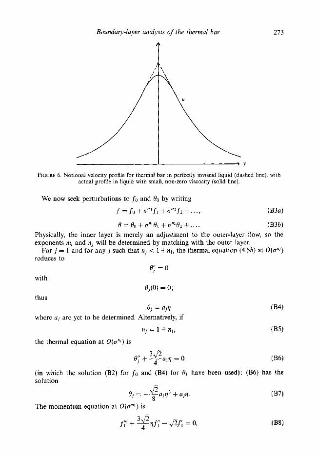
Boundary-layer analysis of the thermal bar 213

RGURE 6. Notional velocity profile for thermal bar in perfectly inviscid liquid (dashed line), with actual profile in liquid with small, non-zero viscosity (solid line).

We now seek perturbations to fo and 00 by writing

f = fo + Drnlfl + arn*f2 + ...) (B3a)

e = eo + dvl + an*t12 + . . . . (B3b) Physically, the inner layer is merely an adjustment to the outer-layer flow, so the exponents mi and n, will be determined by matching with the outer layer.

For j = 1 and for any j such that n, < 1 +nl, the thermal equation (4.5b) at O(O"J) reduces to

with

thus

where a j are yet to be determined. Alternatively, if

or.' = 0

ej(o) = 0 ;

0, = ajq 034)

J

the

(in

nj = 1 + nl,

thermal equation at O(anj) is

which the solution (B2) for fo and (B4) for O1 have been used): (B6) has the solution

1 ~ 3 + ajq. 0. ----a 4

J - 8 The momentum equation at O(arnl) is

fy + hEqf;' - J3f; = 0, 4

2 74 A. Kay, H . K. Kuiken and J. H . Merkin

in which the leading-order solution (Bl), (B2) has been used and it has also been assumed that ml # 2nj for any j .

The solution to (B8), subject to

fl(0) = 0, fl(0) = 0

and the requirement that f should not be exponentially large as q --f co, may be obtained in terms of confluent hypergeometric functions (Slater 1960):

where bl is yet to be determined.

and

f l - i*r17/3 (1 +

From (B9) we have that

f ' l(0) = bl

where

(BlOa)

(Blob)

At higher order (i 2 2) the momentum eqution at O(o"2) is of the form (B8) if mi < 2m1 and mi # 2nj for any j ; however, if

mi = 2nj. (B11)

for some j' with dj. of the form (B4), a term

is added to the right-hand side of (B8). In this case fi will consist of a particular integral

(satisfying fi(0) = 0 and f;(O) = 0), added to a complementary function of the form (B9) with a different constant bi.

Outer-layer variables are to be defined as

0 = 6 , @=oaf, Y = d q ; (B13a)

no rescaling is required for the temperature because it is of order unity at the edge of the inner layer. We require a balance between buoyancy and inertia in the momentum equation and between convection and conduction in the thermal equation : on transforming (4.5) by (B13a) these requirements yield

a = l 2' P = l 2'

so that equations (4.5) become

(B13b)

Boundary-layer analysis of the thermal bar 275

where primes now denote differentiation with respect to Y. Equations (B14a,b) are the forms that the governing equations would have taken if K had been used instead of v in the original definitions of similarity variables (4.2), (4.3); this reflects the fact that K represents the greater of the two diffusive processes in the case under consideration. The outer boundary conditions are

@ + O , 0 - 0 as Y +XI, (B15)

while matching conditions as Y -+ 0 are obtained by expressing the inner-layer solution in terms of outer variables by means of (B13). The leading-order inner-layer solution (B2) yields

@ - & Y as Y + O ;

a solution of form (B10) appearing at O(oml) in (B3a) contributes a term

6 1 a m ~ - 2 / 3 y7/3

to @, while the expression (B12) at O(am2) contributes a term

If these terms are all to match with the leading-order outer solution @o, we require

ml = 2 3 , m2 = 1.

Similarly, requiring solutions of form (B4) and (B7) for 6 at O(anl) and O(an2), respectively, to match with 00 yields

3 n1 = t , n2 = z. Thus, according to the condition (Bll) , the particular integral (B12) is required at O(a), with j' = 1.

The leading-order problem in the outer layer is thus

(B18a)

0; + i@o@;, = 0, (B18b)

(B19a)

(B19b)

@; + O , @ o + O as Y +a. (B20)

The matching conditions (B19) are used to start the numerical integration of (B18) at a small but non-zero value of Y , this being necessary because of the singularity in (B18a) as Y -+ 0 (Merkin 1989); we obtain

a1 = -0.65538, 61 = -0.62013, @O(XI) = 1.58609. (B2 1 a-c)

To obtain higher-order terms in the outer layer, we consider further the matching requirements with the inner-layer solution, which have so far been obtained as

276 A. Kay, H . K. Kuiken and J. H . Merkin

+a a: -q2 + 2q + &q7l3 (1 + O ( V - ~ ) ) as q -+ co, (B22a)

(B22b)

the possibility that further terms exist, of lower order in a than the highest shown, is not yet excluded. In outer variables, the final term in (B22a) becomes

{(f ) I 0 = 1 + 01/2alq + 0 3 / 2 ( --$alq3 8 + a2V) + . . . ;

a '/3E2 y 7/3, (B23)

suggesting that we look for a solution of (B14) at O ( d 3 ) , with

Q, = @o + O ' / ~ Q , ~ + . . . , (B24a)

@ = @ o+a1/301 +.... (B24b) Now, we have seen that inner-layer solutions at orders 0 < a < are of form

0j 0~ q ;

in particular, since q = o - ' / ~ Y , such a solution at O(a5l6) would provide a matching condition at O(O' /~) in 0:

-a3Y as Y +0, (B25) while (B23) gives the behaviour of as Y + 0; the constants a3 and 6 2 are yet to be determined. Substitution of (B24) into the outer-layer equations (B14) yields at O ( C T ' / ~ ) a pair of equations which are linear and homogeneous in Qil and 0 1 ; with the outer boundary conditions of form (B15), the trivial solution

@1 =o , 0, r O

In contrast, if we look for terms of O(a) in the outer layer, replacing (B24) with

Q, = Qio + O@l + . . . ,

is then admitted, setting a3 = 6 2 = 0.

(B26a)

0 = 0 0 + 0 0 1 + ..., then (B22a) yields a matching condition

56 - Q,1 - ~ +..

27 8

(B26b)

containing non-zero constants (see (B21)). The O ( O ~ / ~ ) solution (B7) for 6 in the inner layer yields the matching condition

0 -uzY as Y +O. (B28)

The outer-layer equations at O(o) are (from (B14))

201 - 20001 + &@; + $@b'@1- @p; + (#j: = 0,

0; + ;CPo0; + p10; = 0,

(B29a)

(B29b)

Boundary-layer analysis of the thermal bar

which may be solved numerically to yield

a2 = 0.039681, @(a) = 0.270205.

277

Using the solutions derived above (including the numerically evaluated constants) in the inner and outer expansions (B3) and (B26), we obtain the asymptotic behaviour of the important flow and heat transfer parameters given in (4.11).

REFERENCES

BROOKS, I. & LICK, W. 1972 Lake currents associated with the thermal bar. J. Geophys. Res. 77,

CARMACK, E. C. 1979 Combined influence of inflow and lake temperatures on Spring circulation in

CORMACK, D. E., LEAL, L. G. & IMBERGER, J. 1974 Natural convection in a shallow cavity with

ELLIOT, G. H. 1971 A mathematical study of the thermal bar. In Proc. 14'h Conj Great Lakes Res.,

FARROW, D. E. 199% An asymptotic model for the hydrodynamics of the thermal bar. J . Fluid

FARROW, D. E. 1995b A numerical model of the hydrodynamics of the thermal bar. J . Fluid Mech.

FOREL, F. A. 1880 La congklation des lacs suisses et savoyards pendant l'hiver 1879-1880. $11. Lac

GARRETT, C. & HORNE, E. 1978 Frontal circulation due to cabbeling and double diffusion. J.

GEBHART, B., JALURIA, Y., MAHAJAN, R. L. & SAMMAKIA, B. 1988 Bouyancy-Induced Flows and

GEBHART, B. & MOLLENDORF, J. C. 1977 A new density relation for pure and saline water. Deep-sea

GEBHART, B. & MOLLENDORF, J. C. 1978 Buoyancy induced flows in water under conditions in

HUANG, J. C. K. 1972 The thermal bar. Geophys. Fluid. Dyn. 3, 1-25. HUBBARD, D. W. & SPAIN, J. D. 1973 The structure of the early Spring thermal bar in Lake Superior.

In Proc. 16th Con$ Great Lakes Res., pp. 735-742. Ann Arbor, Michigan: Intl Assoc. Great Lakes Res.

IVEY, G. N. & HAMBLIN, P. F. 1989 Convection near the temperature of maximum density for high Rayleigh number, low aspect ratio, rectangular cavities. Trans. ASME C: J . Heat Transfer 111, 100-105 (referred to herein as IH).

6OOC-6013.

a riverine lake. J. Phys. Oceanogr. 9, 422-434.

differentially heated end walls. Part 1. Asymptotic theory. J. Fluid Mech. 65, 209-229.

pp. 545-554. Ann Arbor, Michigan: Intl Assoc. Great Lakes Res.

Mech. 289, 129-140.

303,279-295.

Lbman. L'Echo des A l p s 3, 149-161.

Geophys. Res. 83,4651-4656.

Transport. Hemisphere.

Res. 24, 831-848.

which density extrema may arise. J . Fiuid. Mech. 89, 673-707.

KUIKEN, H. K. 1969 Free convection at low Prandtl numbers. J . Fluid. Mech. 37, 785-798. KUIKEN, H. K. & ROTEM, Z . 1971 Asymptotic solution for plume at very large and small Prandtl

numbers. J . Fluid. Mech. 45, 585-600. LIN, D. S. & NANSTEEL, M. W. 1987 Natural convection heat transfer in a square enclosure

containing water near its density maximum. Intl J. Heat Mass Transfer 30, 2319-2329. MARMOUSH, Y. R., SMITH, A. A. & HAMBLIN, P. F. 1984 Pilot experiments on thermal bar in lock

exchange flow. J. Energy Engng ASCE. 110,215-227. MERKIN, J. H. 1989 Free convection on a heated vertical plate: the solution for small Prandtl

number. J. Engng Maths 23, 273-282. MOORE, D. R. & WEISS, N. 0. 1973 Non linear penetrative convection. J . Fluid. Mech. 61, 553-581. MORTON, B. R., TAYLOR, G. & TURNER, J. S. 1956 Turbulent gravitational convection from main-

tained and instantaneous sources. Proc. R. SOC. Lond. A 234, 1-23. OSTRACH, S. 1953 An analysis of laminar free-convection flow and heat transfer about a flat plate

parallel to the direction of the generating body force. NACA Rep. 1111. SIMPSON, J. E. 1987 Gravity Currents in the Environment and the Laboratory. Ellis Horwood. SLATER, L. 1960 Confluent Hypergeometric Functions. Cambridge University Press.

278

TURNER, J.S. 1973 Buoyancy Eflects in Fluids. Cambridge University Press. VAN DYKE, M. 1964 Perturbation Methods in Fluid Mechanics. Academic Press. WATSON, A. 1972 Effect of inversion temperature on convection of water in an enclosed rectangular

WITTE, E. 1902 Zur Theorie der Stromkabbelungen. Gaea 38, 484-487. ZILITINKEVICH, S. S., KREIMAN, K. D. & BRZHEVIK, A. Yu. 1992 The thermal bar. J . Fluid. Mech.

A. Kay, H . K . Kuiken and J. H . Merkin

cavity. Q. J . Mech. Appl. Maths 25, 423446.

236,2742.