Nikolay Robinzonov, Gerhard Tutz & Torsten Hothorn

Boosting Techniques for NonlinearTime Series Models

Technical Report Number 075, 2010Department of StatisticsUniversity of Munich

http://www.stat.uni-muenchen.de

Boosting Techniques for Nonlinear Time Series Models

Nikolay Robinzonov1 Gerhard Tutz1 Torsten Hothorn1,∗

1Institut fur Statistik, Ludwig-Maximilians-Universitat MunchenLudwigstraße 33, D–80539 Munchen, Germany

Abstract

Many of the popular nonlinear time series models require a priori the choice of parametricfunctions which are assumed to be appropriate in specific applications. This approach is usedmainly in financial applications, when sufficient knowledge is available about the nonlinearstructure between the covariates and the response. One principal strategy to investigate abroader class on nonlinear time series is the Nonlinear Additive AutoRegressive (NAAR) model.The NAAR model estimates the lags of a time series as flexible functions in order to detect non-monotone relationships between current observations and past values. We consider linear andadditive models for identifying nonlinear relationships. A componentwise boosting algorithmis applied to simultaneous model fitting, variable selection, and model choice. Thus, with theapplication of boosting for fitting potentially nonlinear models we address the major issues intime series modelling: lag selection and nonlinearity. By means of simulation we compare theoutcomes of boosting to the outcomes obtained through alternative nonparametric methods.Boosting shows an overall strong performance in terms of precise estimations of highly nonlinearlag functions. The forecasting potential of boosting is examined on real data where the targetvariable is the German industrial production (IP). In order to improve the model’s forecastingquality we include additional exogenous variables. Thus we address the second major aspectin this paper which concerns the issue of high-dimensionality in models. Allowing additionalinputs in the model extends the NAAR model to an even broader class of models, namelythe NAARX model. We show that boosting can cope with large models which have manycovariates compared to the number of observations.

keywords: componentwise boosting, forecasting, nonlinear times series, autoregressive additivemodels, lag selection.

∗Corresponding author. Email: Torsten.Hothorn@stat.uni-muenchen.de, Tel.: +49 89 2180 6407, Fax: +49 892180 5040

1 INTRODUCTION

1 Introduction

An essential property of a time series is its unknown evolution over time. Some paths are moreprobable than others and this motivates researchers to try to understand the data generating processand possibly to forecast future events. Linear models provide a starting point for modelling thenature of time series. Linear time series models, however, encounter various limitations in the realworld and are applicable only under very restrictive conditions. The field of time series has witnessedvarious new developments in the past two decades which has relaxed some of these constraints. Inparticular, the development of nonparametric regression added more flexibility to standard linearregression adopted by the time series paradigm, see for example Lewis and Stevens (1991), Chenand Tsay (1993), or Huang and Yang (2004). A leading aspect to be explored throughout thispaper is the nonparametric modelling and the resulting forecasting techniques.

The second major aspect concerns the issue of high-dimensionality in the models, i.e., modelstaking potentially many covariates into account. Boosting, one of the most influential strategiesthat deal with high-dimensional models, has its roots in machine learning. The idea has undergonesignificant evolution in the last decade. It has been successfully applied to statistical model fitting(e.g., Buhlmann and Hothorn, 2007). The novel component of the present work is the applicationof boosting to time series, where nonlinear functions of lagged values of a time series have to beestimated.

Due to the frequent use of the simple univariate autoregressive model (AR), we draw on it asa benchmark in the application part to follow. For a substantially broader discussion on timesseries, see Hamilton (1994). In addition we consider the vector autoregressive (VAR) model. TheVAR model suggests that every variable is a linear combination of its past observations and thepast observations of supplemental variables. In practice such assumptions enjoy great popularity.Multivariate time series are considered in greater depth by Lutkepohl (1991, 2006).

The literature offers a great amount of nonlinear modelling tools. Many of them are developed inthe spirit of nonlinear parametric models. They require an a priori choice of parametric functions,which are assumed to be appropriate in specific situations. That approach is used mainly infinancial applications, when sufficient knowledge is available about the nonlinear structure betweenthe covariates and the response. However, the appropriateness of such assumptions is usually hardto justify in practice.

In contrast to parametric nonlinear models, nonparametric techniques are not restricted toa particular choice of parametric functions. One principal strategy is to study the times seriescounterpart of the additive model; the so-called Nonlinear Additive AutoRegressive (NAAR) model(Chen and Tsay, 1993). When further (exogenous) variables are available, we suitably extend themodel with more functions and call it NAARX (Chen and Tsay, 1993). Thus, NAARX encompasseslinear regressive models and many nonlinear models as special cases.

The literature on nonlinear additive models is extensive, therefore, we concentrate on nonpara-metric approaches. Huang and Yang (2004) recently introduced a method that attracted muchattention because of appealing lag-selection properties for univariate nonlinear time series. It es-sentially represents an additive version of the linear stepwise procedure using truncated splines orB-Splines as base expansions of the predictors. The proposed base functions are not penalized.Instead, a formula is suggested which determines a relatively small number of evenly spaced knots.In terms of lag selection, the proposed method performed quite well with simulated time series.However, no results were provided that show the goodness-of-fit of models. We will use some of theartificial times series, provided by Huang and Yang (2004) in Section 3.2 and will shed light upon

2

2 BOOSTING LINEAR AND ADDITIVE MODELS

the goodness-of-fit as well.Multivariate Adaptive Regression Splines (MARS) were introduced by Friedman (1991). A

neat overview of the method is available in Hastie et al. (2001), Hastie, Tibshirani and Friedman(2009, Chapter 9) and an application of MARS in a time series context is provided by Lewisand Stevens (1991). The last nonparametric model that we consider is the BRUTO procedure(Hastie and Tibshirani, 1990, Chapter 9). BRUTO combines inputs selection with backfitting byusing smoothing splines. It was applied to time series by Chen and Tsay (1993). See Hastie andTibshirani (1990, p. 90-91) for details concerning backfitting and Hastie and Tibshirani (1990,p. 262) for the BRUTO algorithm.

We proceed as follows. In Section 2, we shortly review the general ideas of boosting. We adoptthe statistical view on boosting, which is considered purely a numerical optimization, rather thana “traditional” statistical model. Exemplified by two weak learners, we examine the structure ofthe boosting algorithm for continuous data. The first weak learner is a simple linear models, thesecond weak learner is a penalized B-Spline (Eilers and Marx, 1996).

Section 3 examines the results of a simulation study. We analyze the performance of boostingwith P-Spline weak learners in Monte Carlo simulations with six artificial, nonlinear, autoregressivetime series. We compare the outcomes of boosting to the outcomes obtained through alternativenonparametric methods. Their performances are considered in terms of lag-selection and goodness-of-fit.

In Section 4 we apply boosting, both with linear and additive learners, to real world datain terms of forecasting. The target variable is the German industrial production. We compareboosting, along with other methods, to the simple univariate autoregressive model.

2 Boosting Linear and Additive Models

Boosting, in its famous AdaBoost formulation, was developed by Freund and Schapire (1996).Friedman (2001) embedded this algorithm into the framework of functional gradient descent opti-mization for function estimation and made connections to statistical model fitting, for example tologistic regression. Buhlmann and Yu (2003) established componentwise boosting as a means offitting generalized linear and additive models. This seminal paper showed that boosting procedurescan be used to fit a huge class of classical and modern statistical models. For an overview onboosting in general we refer to Buhlmann and Hothorn (2007).

2.1 Steepest Descent

The statistical framework developed by Friedman (2001) interprets boosting as a method for directfunction estimation. He shows that boosting can be interpreted as a basis expansion, in which everysingle basis term is iteratively refitted. Still, some care must be taken in interpreting boosting as abasis expansion. In contrast to conventional basis expansions, where the basis functions are knownin advance, the basis’s members and also their number are iteratively determined by the fittingprocedure. Our notation is as follows:

zt = (y>t ,x>t )> = (yt−1, . . . , yt−p, x

(1)t−1, . . . , x

(1)t−p, . . . , x

(q)t−1, . . . , x

(q)t−p)> ∈ R(q+1)p

denotes the p-lagged vector of explanatory variables representing the lagged values yt = (yt−1, . . . , yt−p)> ∈Rp of the endogenous variable yt ∈ R and the lagged values of q exogenous variables xt ∈ Rqp. The

3

2.1 Steepest Descent 2 BOOSTING LINEAR AND ADDITIVE MODELS

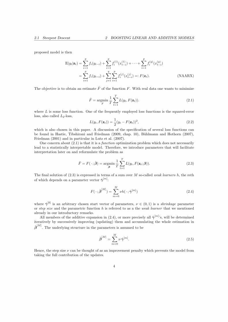
proposed model is then

E(yt|zt) =p∑

i=1

fi(yt−i) +p∑

i=1

f(1)i (x(1)

t−i) + · · ·+p∑

i=1

f(q)i (x(q)

t−i)

=p∑

i=1

fi(yt−i) +q∑

j=1

p∑i=1

f(j)i (x(j)

t−i) =: F (zt). (NAARX)

The objective is to obtain an estimate F of the function F . With real data one wants to minimize

F = argminF

1T

T∑t=1

L(yt, F (zt)). (2.1)

where L is some loss function. One of the frequently employed loss functions is the squared-errorloss, also called L2-loss,

L(yt, F (zt)) =12

(yt − F (zt))2, (2.2)

which is also chosen in this paper. A discussion of the specification of several loss functions canbe found in Hastie, Tibshirani and Friedman (2009, chap. 10), Buhlmann and Hothorn (2007),Friedman (2001) and in particular in Lutz et al. (2007).

One concern about (2.1) is that it is a function optimization problem which does not necessarilylead to a statistically interpretable model. Therefore, we introduce parameters that will facilitateinterpretation later on and reformulate the problem as

F = F ( · ; β) = argminβ

1T

T∑t=1

L(yt, F (zt; β)). (2.3)

The final solution of (2.3) is expressed in terms of a sum over M so-called weak learners h, the mthof which depends on a parameter vector γ[m]:

F ( · ; β[M ]) =

M∑m=0

νh( · ; γ[m]) (2.4)

where γ[0] is an arbitrary chosen start vector of parameters, ν ∈ (0, 1) is a shrinkage parameteror step size and the parametric function h is referred to as a the weak learner that we mentionedalready in our introductory remarks.

All members of the additive expansion in (2.4), or more precisely all γ[m]’s, will be determinediteratively by successively improving (updating) them and accumulating the whole estimation in

β[M ]

. The underlying structure in the parameters is assumed to be

β[M ]

=M∑

m=0

ν γ[m]. (2.5)

Hence, the step size ν can be thought of as an improvement penalty which prevents the model fromtaking the full contribution of the updates.

4

2.2 Componentwise Boosting 2 BOOSTING LINEAR AND ADDITIVE MODELS

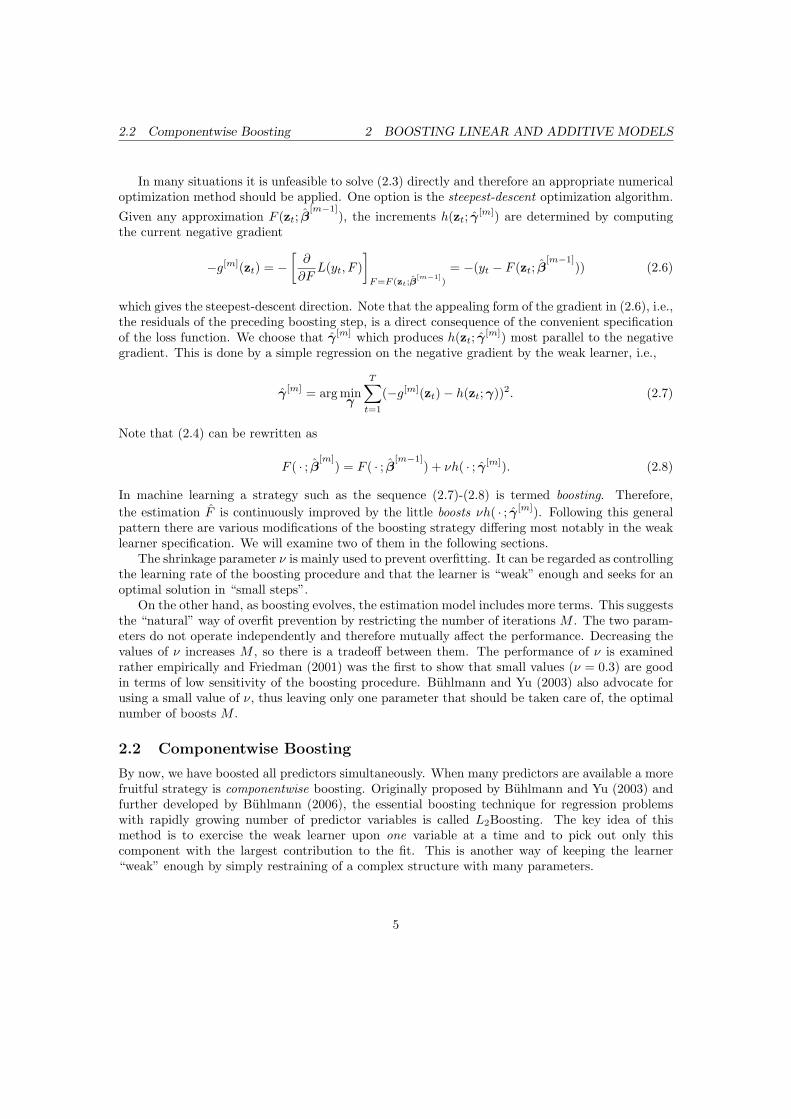
In many situations it is unfeasible to solve (2.3) directly and therefore an appropriate numericaloptimization method should be applied. One option is the steepest-descent optimization algorithm.

Given any approximation F (zt; β[m−1]

), the increments h(zt; γ[m]) are determined by computing

the current negative gradient

−g[m](zt) = −[∂

∂FL(yt, F )

]F=F (zt;β

[m−1])

= −(yt − F (zt; β[m−1]

)) (2.6)

which gives the steepest-descent direction. Note that the appealing form of the gradient in (2.6), i.e.,the residuals of the preceding boosting step, is a direct consequence of the convenient specificationof the loss function. We choose that γ[m] which produces h(zt; γ

[m]) most parallel to the negativegradient. This is done by a simple regression on the negative gradient by the weak learner, i.e.,

γ[m] = arg minγ

T∑t=1

(−g[m](zt)− h(zt; γ))2. (2.7)

Note that (2.4) can be rewritten as

F ( · ; β[m]) = F ( · ; β[m−1]

) + νh( · ; γ[m]). (2.8)

In machine learning a strategy such as the sequence (2.7)-(2.8) is termed boosting. Therefore,the estimation F is continuously improved by the little boosts νh( · ; γ[m]). Following this generalpattern there are various modifications of the boosting strategy differing most notably in the weaklearner specification. We will examine two of them in the following sections.

The shrinkage parameter ν is mainly used to prevent overfitting. It can be regarded as controllingthe learning rate of the boosting procedure and that the learner is “weak” enough and seeks for anoptimal solution in “small steps”.

On the other hand, as boosting evolves, the estimation model includes more terms. This suggeststhe “natural” way of overfit prevention by restricting the number of iterations M . The two param-eters do not operate independently and therefore mutually affect the performance. Decreasing thevalues of ν increases M , so there is a tradeoff between them. The performance of ν is examinedrather empirically and Friedman (2001) was the first to show that small values (ν = 0.3) are goodin terms of low sensitivity of the boosting procedure. Buhlmann and Yu (2003) also advocate forusing a small value of ν, thus leaving only one parameter that should be taken care of, the optimalnumber of boosts M .

2.2 Componentwise Boosting

By now, we have boosted all predictors simultaneously. When many predictors are available a morefruitful strategy is componentwise boosting. Originally proposed by Buhlmann and Yu (2003) andfurther developed by Buhlmann (2006), the essential boosting technique for regression problemswith rapidly growing number of predictor variables is called L2Boosting. The key idea of thismethod is to exercise the weak learner upon one variable at a time and to pick out only thiscomponent with the largest contribution to the fit. This is another way of keeping the learner“weak” enough by simply restraining of a complex structure with many parameters.

5

2.2 Componentwise Boosting 2 BOOSTING LINEAR AND ADDITIVE MODELS

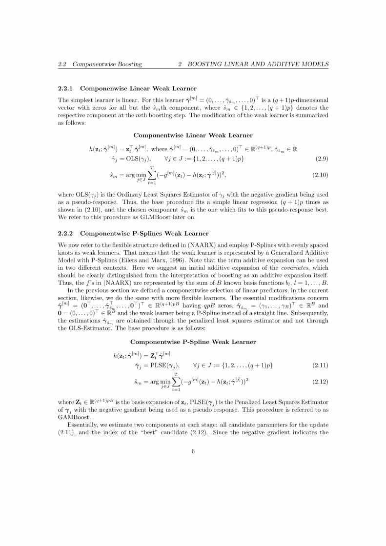
2.2.1 Componenwise Linear Weak Learner

The simplest learner is linear. For this learner γ[m] = (0, . . . , γsm , . . . , 0)> is a (q+ 1)p-dimensionalvector with zeros for all but the smth component, where sm ∈ {1, 2, . . . , (q + 1)p} denotes therespective component at the mth boosting step. The modification of the weak learner is summarizedas follows:

Componentwise Linear Weak Learner

h(zt; γ[m]) = z>t γ[m], where γ[m] = (0, . . . , γsm

, . . . , 0)> ∈ R(q+1)p, γsm∈ R

γj = OLS(γj), ∀j ∈ J := {1, 2, . . . , (q + 1)p} (2.9)

sm = arg minj∈J

T∑t=1

(−g[m](zt)− h(zt; γ[j]))2, (2.10)

where OLS(γj) is the Ordinary Least Squares Estimator of γj with the negative gradient being usedas a pseudo-response. Thus, the base procedure fits a simple linear regression (q + 1)p times asshown in (2.10), and the chosen component sm is the one which fits to this pseudo-response best.We refer to this procedure as GLMBoost later on.

2.2.2 Componentwise P-Splines Weak Learner

We now refer to the flexible structure defined in (NAARX) and employ P-Splines with evenly spacedknots as weak learners. That means that the weak learner is represented by a Generalized AdditiveModel with P-Splines (Eilers and Marx, 1996). Note that the term additive expansion can be usedin two different contexts. Here we suggest an initial additive expansion of the covariates, whichshould be clearly distinguished from the interpretation of boosting as an additive expansion itself.Thus, the f ’s in (NAARX) are represented by the sum of B known basis functions bl, l = 1, . . . , B.

In the previous section we defined a componentwise selection of linear predictors, in the currentsection, likewise, we do the same with more flexible learners. The essential modifications concernγ[m] = (0>, . . . , γ>sm

, . . . ,0>)> ∈ R(q+1)pB having qpB zeros, γ sm= (γ1, . . . , γB)> ∈ RB and

0 = (0, . . . , 0)> ∈ RB and the weak learner being a P-Spline instead of a straight line. Subsequently,the estimations γ sm

are obtained through the penalized least squares estimator and not throughthe OLS-Estimator. The base procedure is as follows:

Componentwise P-Spline Weak Learner

h(zt; γ[m]) = Z>t γ[m]

γj = PLSE(γj), ∀j ∈ J := {1, 2, . . . , (q + 1)p} (2.11)

sm = arg minj∈J

T∑t=1

(−g[m](zt)− h(zt; γ[j]))2 (2.12)

where Zt ∈ R(q+1)pB is the basis expansion of zt, PLSE(γj) is the Penalized Least Squares Estimatorof γj with the negative gradient being used as a pseudo response. This procedure is referred to asGAMBoost.

Essentially, we estimate two components at each stage: all candidate parameters for the update(2.11), and the index of the “best” candidate (2.12). Since the negative gradient indicates the

6

3 SIMULATION STUDY

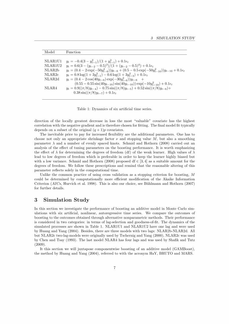
Model Function

NLAR1U1 yt = −0.4(3− y2t−1)/(1 + y2

t−1) + 0.1εtNLAR1U2 yt = 0.6(3− (yt−2 − 0.5)3)/(1 + (yt−2 − 0.5)4) + 0.1εtNLAR2b yt = (0.4− 2 exp(−50y2

t−6))yt−6 + (0.5− 0.5 exp(−50y2t−10))yt−10 + 0.1εt

NLAR2c yt = 0.8 log(1 + 3y2t−1)− 0.6 log(1 + 3y2

t−3) + 0.1εtNLAR2d yt = (0.4− 2 cos(40yt−6) exp(−30y2

t−6))yt−6 +(0.55− 0.55 sin(40yt−10) sin(40yt−10)) exp(−10y2

t−10) + 0.1εtNLAR4 yt = 0.9((π/8)yt−4)− 0.75 sin((π/8)yt−5) + 0.52 sin((π/8)yt−6)+

0.38 sin((π/8)yt−7) + 0.1εt

Table 1: Dynamics of six artificial time series.

direction of the locally greatest decrease in loss the most “valuable” covariate has the highestcorrelation with the negative gradient and is therefore chosen for fitting. The final model fit typicallydepends on a subset of the original (q + 1)p covariates.

The inevitable price to pay for increased flexibility are the additional parameters. One has tochoose not only an appropriate shrinkage factor ν and stopping value M , but also a smoothingparameter λ and a number of evenly spaced knots. Schmid and Hothorn (2008) carried out ananalysis of the effect of tuning parameters on the boosting performance. It is worth emphasizingthe effect of λ for determining the degrees of freedom (df) of the weak learner. High values of λlead to low degrees of freedom which is preferable in order to keep the learner highly biased butwith a low variance. Schmid and Hothorn (2008) proposed df ∈ [3, 4] as a suitable amount for thedegrees of freedom. We follow these prescriptions and remind that the reasonable altering of thisparameter reflects solely in the computational time.

Unlike the common practice of using cross validation as a stopping criterion for boosting, Mcould be determined by computationally more efficient modification of the Akaike InformationCriterion (AICs, Hurvich et al. 1998). This is also our choice, see Buhlmann and Hothorn (2007)for further details.

3 Simulation Study

In this section we investigate the performance of boosting an additive model in Monte Carlo sim-ulations with six artificial, nonlinear, autoregressive time series. We compare the outcomes ofboosting to the outcomes obtained through alternative nonparametric methods. Their performanceis considered in two categories: in terms of lag-selection and goodness-of-fit. The dynamics of thesimulated processes are shown in Table 1. NLAR1U1 and NLAR1U2 have one lag and were usedby Huang and Yang (2004). Besides, there are three models with two lags: NLAR2b-NLAR2d. Allbut NLAR2c two-lag-models were originally used by Tschernig and Yang (2000), NLAR2c was usedby Chen and Tsay (1993). The last model NLAR4 has four lags and was used by Shafik and Tutz(2009).

It this section we will juxtapose componentwise boosting of an additive model (GAMBoost),the method by Huang and Yang (2004), referred to with the acronym HaY, BRUTO and MARS.

7

3.1 Lag Selection 3 SIMULATION STUDY

All models from Table 1 have been simulated 100 times with sizes 400 + N , the first 400values discarded and N = p + T , with p = 10 pre-sample values and T = 50, 100, 200 in-sampleobservations. Such partitioning of the time series values is convenient in order to ensure samesample size of T for each covariate at a given period and to simplify the notation. As p suggests,the maximal lag-length has been limited to ten. In the next section we compare the performanceof the different procedures in terms of lag selection.

3.1 Lag Selection

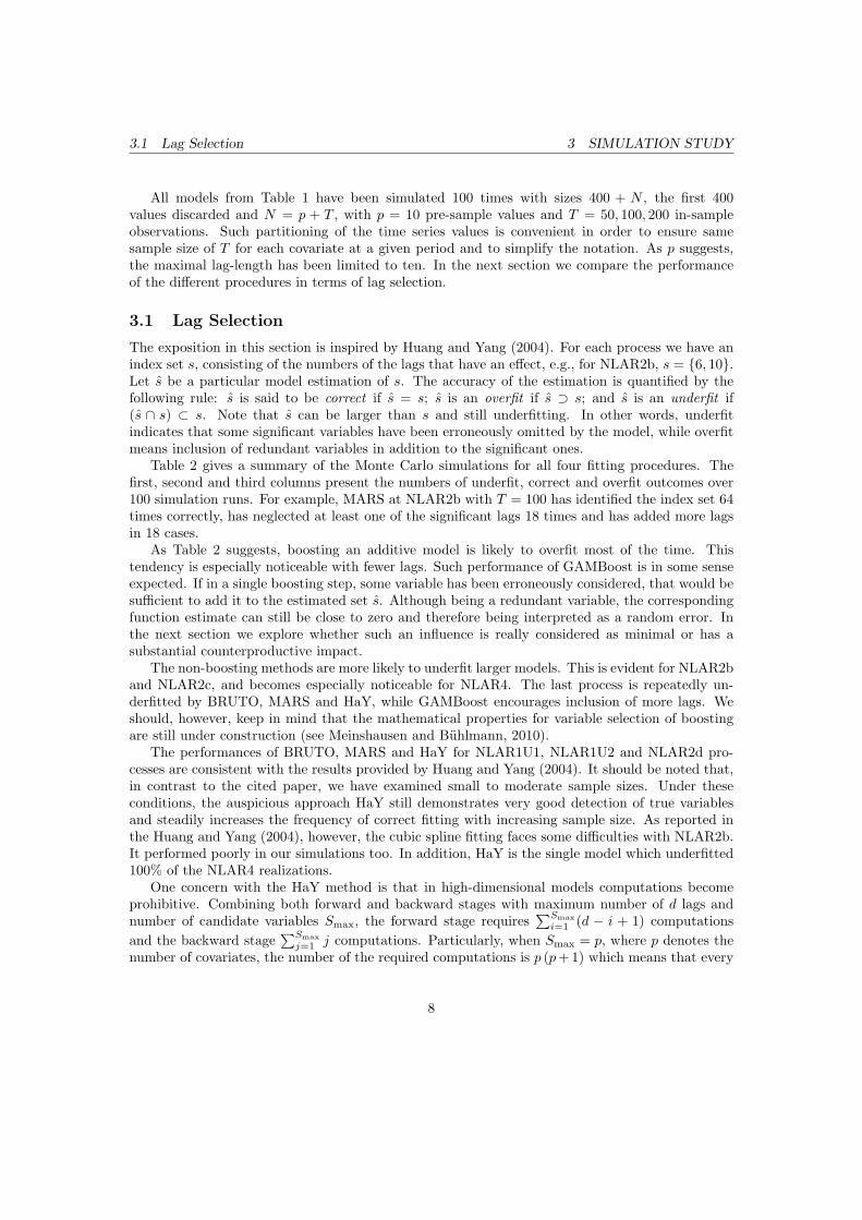
The exposition in this section is inspired by Huang and Yang (2004). For each process we have anindex set s, consisting of the numbers of the lags that have an effect, e.g., for NLAR2b, s = {6, 10}.Let s be a particular model estimation of s. The accuracy of the estimation is quantified by thefollowing rule: s is said to be correct if s = s; s is an overfit if s ⊃ s; and s is an underfit if(s ∩ s) ⊂ s. Note that s can be larger than s and still underfitting. In other words, underfitindicates that some significant variables have been erroneously omitted by the model, while overfitmeans inclusion of redundant variables in addition to the significant ones.

Table 2 gives a summary of the Monte Carlo simulations for all four fitting procedures. Thefirst, second and third columns present the numbers of underfit, correct and overfit outcomes over100 simulation runs. For example, MARS at NLAR2b with T = 100 has identified the index set 64times correctly, has neglected at least one of the significant lags 18 times and has added more lagsin 18 cases.

As Table 2 suggests, boosting an additive model is likely to overfit most of the time. Thistendency is especially noticeable with fewer lags. Such performance of GAMBoost is in some senseexpected. If in a single boosting step, some variable has been erroneously considered, that would besufficient to add it to the estimated set s. Although being a redundant variable, the correspondingfunction estimate can still be close to zero and therefore being interpreted as a random error. Inthe next section we explore whether such an influence is really considered as minimal or has asubstantial counterproductive impact.

The non-boosting methods are more likely to underfit larger models. This is evident for NLAR2band NLAR2c, and becomes especially noticeable for NLAR4. The last process is repeatedly un-derfitted by BRUTO, MARS and HaY, while GAMBoost encourages inclusion of more lags. Weshould, however, keep in mind that the mathematical properties for variable selection of boostingare still under construction (see Meinshausen and Buhlmann, 2010).

The performances of BRUTO, MARS and HaY for NLAR1U1, NLAR1U2 and NLAR2d pro-cesses are consistent with the results provided by Huang and Yang (2004). It should be noted that,in contrast to the cited paper, we have examined small to moderate sample sizes. Under theseconditions, the auspicious approach HaY still demonstrates very good detection of true variablesand steadily increases the frequency of correct fitting with increasing sample size. As reported inthe Huang and Yang (2004), however, the cubic spline fitting faces some difficulties with NLAR2b.It performed poorly in our simulations too. In addition, HaY is the single model which underfitted100% of the NLAR4 realizations.

One concern with the HaY method is that in high-dimensional models computations becomeprohibitive. Combining both forward and backward stages with maximum number of d lags andnumber of candidate variables Smax, the forward stage requires

∑Smaxi=1 (d − i + 1) computations

and the backward stage∑Smax

j=1 j computations. Particularly, when Smax = p, where p denotes thenumber of covariates, the number of the required computations is p (p+ 1) which means that every

8

3.2 Estimation of Dynamics 3 SIMULATION STUDY

Model Length GAMBoost BRUTO MARS HaYNLAR1U1 50 0 3 97 0 29 71 0 73 27 0 98 2

100 0 1 99 0 22 78 0 70 30 0 99 1200 0 1 99 0 26 74 0 79 21 0 100 0

NLAR1U2 50 0 0 100 0 0 100 0 73 27 0 1 99100 0 1 99 0 0 100 0 81 19 0 31 69200 0 0 100 0 0 100 0 72 28 0 71 29

NLAR2b 50 8 0 92 99 1 0 64 29 7 100 0 0100 0 1 99 73 26 1 18 64 18 97 3 0200 0 0 100 5 95 0 0 80 20 98 2 0

NLAR2c 50 42 2 56 100 0 0 86 11 3 99 1 0100 15 1 84 98 2 0 69 24 7 90 10 0200 3 1 96 83 17 0 32 46 22 67 33 0

NLAR2d 50 6 0 94 39 51 10 42 30 28 67 33 0100 0 0 100 12 76 12 5 60 35 28 72 0200 0 0 100 0 93 7 0 75 25 0 100 0

NLAR4 50 86 0 14 100 0 0 100 0 0 100 0 0100 56 0 44 100 0 0 98 2 0 100 0 0200 16 0 84 91 9 0 84 11 5 100 0 0

Table 2: Simulation results for lag selection. The first, second and third columns in each setupshow the number of underfit, correct and overfit outcomes over 100 simulation runs.

covariate contributes quadratically to the computational burden. For high dimensions that wouldbe an essential issue.

MARS showed an overall good performance. It had the highest rate of significant hits withNLAR4 amongst the non-boosting methods. On the other hand, BRUTO showed a rather erraticbehaviour by favouring processes like NLAR2b, NLAR2d and performing very poorly with theothers.

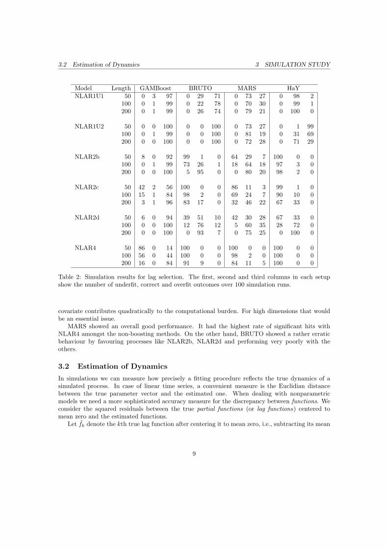
3.2 Estimation of Dynamics

In simulations we can measure how precisely a fitting procedure reflects the true dynamics of asimulated process. In case of linear time series, a convenient measure is the Euclidian distancebetween the true parameter vector and the estimated one. When dealing with nonparametricmodels we need a more sophisticated accuracy measure for the discrepancy between functions. Weconsider the squared residuals between the true partial functions (or lag functions) centered tomean zero and the estimated functions.

Let fk denote the kth true lag function after centering it to mean zero, i.e., subtracting its mean

9

3.2 Estimation of Dynamics 3 SIMULATION STUDY

Model T GAMBoost BRUTO MARS HaY

NLAR1U1 50 0.0228 0.0895 0.0093 0.0027100 0.0141 0.0508 0.0039 0.0020200 0.0080 0.0278 0.0016 0.0014

NLAR1U2 50 0.4035 2.5098 0.4288 0.7184100 0.2380 1.6916 0.3381 0.7289200 0.1789 0.9420 0.3049 0.1622

NLAR2b 50 0.0201 0.0443 0.0393 0.0470100 0.0123 0.0349 0.0140 0.0455200 0.0074 0.0084 0.0078 0.0358

NLAR2c 50 0.0065 0.0077 0.0120 0.0072100 0.0049 0.0074 0.0084 0.0067200 0.0028 0.0054 0.0058 0.0042

NLAR2d 50 0.1154 0.0886 0.1375 0.1260100 0.0925 0.0786 0.0877 0.0766200 0.0788 0.0704 0.0672 0.0699

NLAR4 50 0.0181 0.0247 0.0278 0.0301100 0.0133 0.0176 0.0197 0.0278200 0.0077 0.0085 0.0104 0.0147

Table 3: Simulation results of the median MSPE of 100 simulation runs multiplied by 100. Boldfacenumbers indicate the best model performance for each setup.

value. Then the mean squared prediction error is

MSPEk =1

200

200∑i=1

[fk(zi)− ˆfk(zi)]2 (3.1)

where ˆfk is the estimated counterpart of fk. We choose the zi’s being evenly spaced between the

5th and 95th quantile of the empirical distribution of yt−k. The accuracy measure is the averageof the individual MSPE’s

MSPE =p∑

k=1

MSPEk. (3.2)

The results of the median MSPE across all 100 simulation runs are summarized in Table 3, wherethe rows give the simulated series and the columns represent the different modelling techniques.NLAR1U and NLAR1U2 yield the most parsimonious models. Their dynamics seems to be ex-plained very well by MARS, HaY and GAMBoost, while BRUTO performed very poorly. For

10

3.2 Estimation of Dynamics 3 SIMULATION STUDY

●●●●●●●●●●●●●●●●●●●●

−0.1 0.4 0.9 1.4 1.9

−0.68

−0.34

0.000.00

0.34

0.68

Lag 1

●●●●●●●●●

●

●

●

●

●

●

●

●

●

●

●

−0.1 0.4 0.9 1.4 1.9

−0.68

−0.34

0.000.00

0.34

0.68

Lag 2

●●●●●●●●●●●●●●●●●●●●

−0.1 0.4 0.9 1.4 1.9

−0.68

−0.34

0.000.00

0.34

0.68

Lag 3

●●●●●●●●●●●●●●●●●●●●

−0.1 0.4 0.9 1.4 1.9

−0.68

−0.34

0.000.00

0.34

0.68

Lag 4

●●●●●●●●●●●●●●●●●●●●

−0.1 0.4 0.9 1.4 1.9

−0.68

−0.34

0.000.00

0.34

0.68

Lag 5

●●●●●●●●●●●●●●●●●●●●

−0.1 0.4 0.9 1.4 1.9

−0.68

−0.34

0.000.00

0.34

0.68

Lag 6

●●●●●●●●●●●●●●●●●●●●

−0.1 0.4 0.9 1.4 1.9

−0.68

−0.34

0.000.00

0.34

0.68

Lag 7

●●●●●●●●●●●●●●●●●●●●

−0.1 0.4 0.9 1.4 1.9

−0.68

−0.34

0.000.00

0.34

0.68

Lag 8

●●●●●●●●●●●●●●●●●●●●

−0.1 0.4 0.9 1.4 1.9

−0.68

−0.34

0.000.00

0.34

0.68

Lag 9

●●●●●●●●●●●●●●●●●●●●

−0.1 0.4 0.9 1.4 1.9

−0.68

−0.34

0.000.00

0.34

0.68

Lag 10

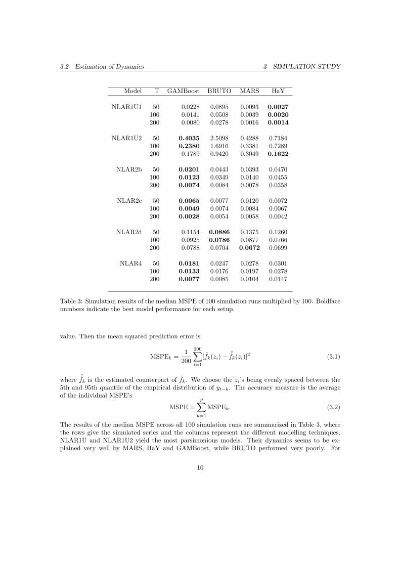
Figure 1: Boosting estimations of the lag functions of NLAR1U2. True lag is 2 (circled line),estimated lags are depicted as solid lines. The functions are mean zero centered.

NLAR1U2, we notice that despite overfitting in sense of selected lags, boosting estimated the rel-evant function quite precisely, e.g., T = 50, 100. This suggests that the redundant functions wereconsidered close to zero. It is reassuring to see the seemingly zero redundant lag estimations ofNLAR1U2 in Figure 1.

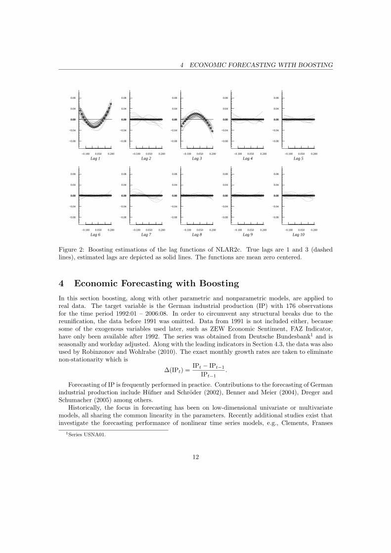
The literature on nonparametric regression for dependent data is relatively sparse, especiallywhen related to boosting. Strong serial dependence might mislead the fitting procedure to produceerroneous transformations. For instance, this is evident for boosting of NLAR2c, shown Figure 2,where the second and the seventh lag were overfitted rather strongly.

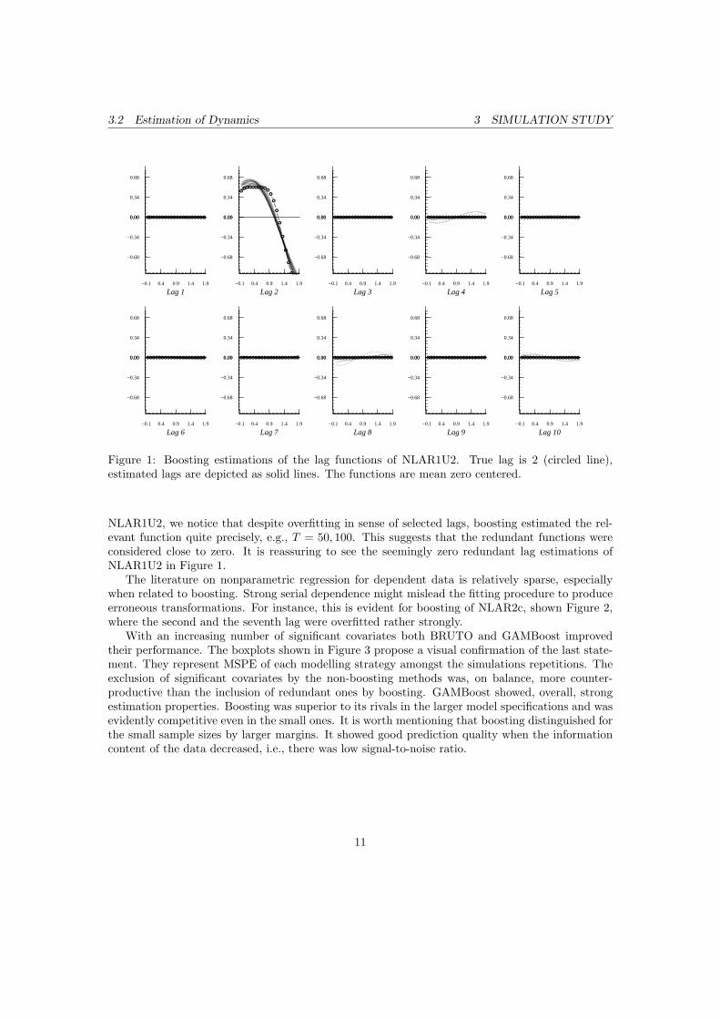
With an increasing number of significant covariates both BRUTO and GAMBoost improvedtheir performance. The boxplots shown in Figure 3 propose a visual confirmation of the last state-ment. They represent MSPE of each modelling strategy amongst the simulations repetitions. Theexclusion of significant covariates by the non-boosting methods was, on balance, more counter-productive than the inclusion of redundant ones by boosting. GAMBoost showed, overall, strongestimation properties. Boosting was superior to its rivals in the larger model specifications and wasevidently competitive even in the small ones. It is worth mentioning that boosting distinguished forthe small sample sizes by larger margins. It showed good prediction quality when the informationcontent of the data decreased, i.e., there was low signal-to-noise ratio.

11

4 ECONOMIC FORECASTING WITH BOOSTING

●

●

●

●

●●

●●●●●

●●

●

●

●

●

●

●

●

−0.100 0.050 0.200

−0.08

−0.04

0.000.00

0.04

0.08

Lag 1

●●●●●●●●●●●●●●●●●●●●

−0.100 0.050 0.200

−0.08

−0.04

0.000.00

0.04

0.08

Lag 2

●

●

●●

●●

●●●●●●●

●●

●

●

●

●

●

−0.100 0.050 0.200

−0.08

−0.04

0.000.00

0.04

0.08

Lag 3

●●●●●●●●●●●●●●●●●●●●

−0.100 0.050 0.200

−0.08

−0.04

0.000.00

0.04

0.08

Lag 4

●●●●●●●●●●●●●●●●●●●●

−0.100 0.050 0.200

−0.08

−0.04

0.000.00

0.04

0.08

Lag 5

●●●●●●●●●●●●●●●●●●●●

−0.100 0.050 0.200

−0.08

−0.04

0.000.00

0.04

0.08

Lag 6

●●●●●●●●●●●●●●●●●●●●

−0.100 0.050 0.200

−0.08

−0.04

0.000.00

0.04

0.08

Lag 7

●●●●●●●●●●●●●●●●●●●●

−0.100 0.050 0.200

−0.08

−0.04

0.000.00

0.04

0.08

Lag 8

●●●●●●●●●●●●●●●●●●●●

−0.100 0.050 0.200

−0.08

−0.04

0.000.00

0.04

0.08

Lag 9

●●●●●●●●●●●●●●●●●●●●

−0.100 0.050 0.200

−0.08

−0.04

0.000.00

0.04

0.08

Lag 10

Figure 2: Boosting estimations of the lag functions of NLAR2c. True lags are 1 and 3 (dashedlines), estimated lags are depicted as solid lines. The functions are mean zero centered.

4 Economic Forecasting with Boosting

In this section boosting, along with other parametric and nonparametric models, are applied toreal data. The target variable is the German industrial production (IP) with 176 observationsfor the time period 1992:01 – 2006:08. In order to circumvent any structural breaks due to thereunification, the data before 1991 was omitted. Data from 1991 is not included either, becausesome of the exogenous variables used later, such as ZEW Economic Sentiment, FAZ Indicator,have only been available after 1992. The series was obtained from Deutsche Bundesbank1 and isseasonally and workday adjusted. Along with the leading indicators in Section 4.3, the data was alsoused by Robinzonov and Wohlrabe (2010). The exact monthly growth rates are taken to eliminatenon-stationarity which is

∆(IPt) =IPt − IPt−1

IPt−1.

Forecasting of IP is frequently performed in practice. Contributions to the forecasting of Germanindustrial production include Hufner and Schroder (2002), Benner and Meier (2004), Dreger andSchumacher (2005) among others.

Historically, the focus in forecasting has been on low-dimensional univariate or multivariatemodels, all sharing the common linearity in the parameters. Recently additional studies exist thatinvestigate the forecasting performance of nonlinear time series models, e.g., Clements, Franses

1Series USNA01.

12

4 ECONOMIC FORECASTING WITH BOOSTING

MSPE*100

0.01

0.02

0.03

0.04

0.05

0.06

BR

UT

OG

AM

Boo

stH

aYM

AR

S

●

●

●

●

● ●● ● ●● ●●● ●

● ●

● ●● ● ●● ●● ● ●

● ● ●

NLA

R2b

, T =

050

BR

UT

OG

AM

Boo

stH

aYM

AR

S

●

●

●

●

●●

●●● ●

● ●●●● ●●

NLA

R2b

, T =

100

BR

UT

OG

AM

Boo

stH

aYM

AR

S

●●

●

●

●●● ● ● ●● ●

● ● ●●

● ●●● ●● ●● ●● ●●● ●● ● ● ●●●

●●

NLA

R2b

, T =

200

MSPE*100

0.5

1.0

1.5

2.0

2.5

3.0

BR

UT

OG

AM

Boo

stH

aYM

AR

S

●

●

●

●

●

● ●

●● ●●

●

NLA

R1U

2, T

= 0

50

BR

UT

OG

AM

Boo

stH

aYM

AR

S

●

●

●

●

●

● ● ●

●●●● ● ●●●

NLA

R1U

2, T

= 1

00

BR

UT

OG

AM

Boo

stH

aYM

AR

S

●

●

●

●

●●●

● ●● ●

● ●● ●

● ●●● ● ●●● ● ●● ●● ●● ●●

NLA

R1U

2, T

= 2

00

MSPE*100

0.05

0.10

0.15

0.20

BR

UT

OG

AM

Boo

stH

aYM

AR

S

●

●

●●

● ● ●● ●●● ●● ●

●● ●● ● ●

● ● ●● ●● ●● ● ●●● ●

NLA

R1U

1, T

= 0

50

BR

UT

OG

AM

Boo

stH

aYM

AR

S

●

●●

●

●

●● ● ● ●●● ●

● ●● ● ●●●● ●●● ●●● ●●●

NLA

R1U

1, T

= 1

00

BR

UT

OG

AM

Boo

stH

aYM

AR

S

●●

●●

●●● ● ●

●●●● ●●●

●● ●●●●● ●●●● ●●● ●●

NLA

R1U

1, T

= 2

00

MSPE*100

0.01

0.02

0.03

0.04

0.05

0.06

BR

UT

OG

AM

Boo

stH

aYM

AR

S

●

●

●●

●● ●● ●● ● ●●●● ● ●

● ●● ●● ●● ●●

● ●● ●

NLA

R4,

T =

050

BR

UT

OG

AM

Boo

stH

aYM

AR

S

●

●

●

●

● ●

● ●● ●● ● ● ●●

●● ● ●

● ● ●●

NLA

R4,

T =

100

BR

UT

OG

AM

Boo

stH

aYM

AR

S

●●

●

●

●●● ● ●

● ●

NLA

R4,

T =

200

MSPE*100

0.05

0.10

0.15

0.20

0.25

BR

UT

OG

AM

Boo

stH

aYM

AR

S

●

●●

●

● ● ●●● ●● ● ● ●● ●

● ● ● ●● ●●●

●● ●● ●● ●●

●●● ●● ● ●● ●●

NLA

R2d

, T =

050

BR

UT

OG

AM

Boo

stH

aYM

AR

S

●●

●●

● ●● ● ● ● ●

● ●●● ●● ●●● ●● ●●

● ●●● ●● ●

NLA

R2d

, T =

100

BR

UT

OG

AM

Boo

stH

aYM

AR

S

●●

●●

● ●● ●● ●● ● ●

●● ●●

●●

NLA

R2d

, T =

200

MSPE*100

0.00

5

0.01

0

0.01

5

0.02

0

0.02

5

BR

UT

OG

AM

Boo

stH

aYM

AR

S

●●

●

●

● ●● ●●●

●● ●● ●● ●

●

NLA

R2c

, T =

050

BR

UT

OG

AM

Boo

stH

aYM

AR

S

●

●

●

●

●●●

● ● ● ●

● ●● ●●● ●● ●

NLA

R2c

, T =

100

BR

UT

OG

AM

Boo

stH

aYM

AR

S

●

●●

●

●

● ● ●●

●● ●●● ● ●

NLA

R2c

, T =

200

Fig

ure

3:B

oxpl

ots

ofth

eM

onte

-Car

losi

mul

atio

ns.

13

4.1 Forecasting Principles 4 ECONOMIC FORECASTING WITH BOOSTING

and Swanson (2004), Terasvirta, van Dijk and Medeiros (2005), Claveria, Pons and Ramos (2007),Elliot and Timmermann (2008). The application of boosting by means of economic forecasting isthe major novelty in the present work.

4.1 Forecasting Principles

When a specific time series model is assumed and a set of observations is given, we want to predict.The given set of observations is called a training set or an information set. The intention is to usethe information in zt to predict the real outputs yt+h.

We use a direct forecasting strategy (e.g. Marcellino et al., 2006, Chevillon and Hendry, 2005).The idea is to use a horizon-specific estimation model, where response is the multiperiod aheadvalue. The approach differs from iterated forecasting. The question which method is preferable isan empirical one. The direct forecasting approach is surely a good choice under the presence ofexogenous variables.

To evaluate accuracy of prediction we need to specify a cost function. The choice of an accuracymeasure is a major topic by itself. Hyndman and Koehler (2006) widely discussed and compareddifferent measures of accuracy of times series forecasts. The references therein point the reader todifferent studies with often controversial conclusions about the “best” forecasting measure. Still,the literature being inconsistent, the MSE withstands the time proof and remains one of the mostpopular out-of-sample measures. Therefore, minimizing the quadratic expected cost or loss

MSE = E (yt+h − yt+h|zt)2 (4.1)

is set as an objective. Expression (4.1) is known as the mean squared error, associated with theforecast yt+h.

Further we are interested in obtaining estimations of multiple forecasting horizons. Therefore,we alter the information set consistently. One option is to fix the starting point of the informationset and consecutively enlarge its size with new observations. This method is called recursive schemefor forecasting. We apply the direct type of forecasting with the above mentioned recursive schemeto all models in the remaining part of this paper.

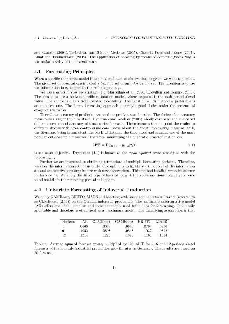
4.2 Univariate Forecasting of Industrial Production

We apply GAMBoost, BRUTO, MARS and boosting with linear componentwise learner (referred toas GLMBoost, (2.10)) on the German industrial production. The univariate autoregressive model(AR) offers one of the simplest and most commonly used techniques for forecasting. It is easilyapplicable and therefore is often used as a benchmark model. The underlying assumption is that

Horizon AR GLMBoost GAMBoost BRUTO MARS1 .0668 .0648 .0698 .0704 .09166 .1052 .0808 .0848 .1037 .089212 .1214 .1220 .1093 .1161 .1014

Table 4: Average squared forecast errors, multiplied by 103, of IP for 1, 6 and 12-periods aheadforecasts of the monthly industrial production growth rates in Germany. The results are based on20 forecasts.

14

4.2 Forecasting I 4 ECONOMIC FORECASTING WITH BOOSTINGM

SE

x 1

000

0.0

0.1

0.2

0.3

0.4

AR

BRUTO

GAMBoo

st

GLMBoo

st

MARS

● ● ●●

●

●

● ●●

●

Horizon = 1

AR

BRUTO

GAMBoo

st

GLMBoo

st

MARS

● ●

● ● ●

Horizon = 6

AR

BRUTO

GAMBoo

st

GLMBoo

st

MARS

●●

●●

●

●●

●

Horizon = 12

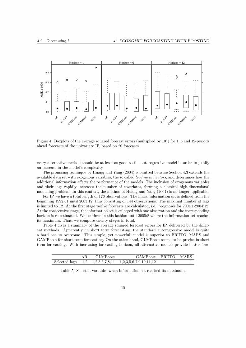
Figure 4: Boxplots of the average squared forecast errors (multiplied by 103) for 1, 6 and 12-periodsahead forecasts of the univariate IP, based on 20 forecasts.

every alternative method should be at least as good as the autoregressive model in order to justifyan increase in the model’s complexity.

The promising technique by Huang and Yang (2004) is omitted because Section 4.3 extends theavailable data set with exogenous variables, the so called leading indicators, and determines how theadditional information affects the performance of the models. The inclusion of exogenous variablesand their lags rapidly increases the number of covariates, forming a classical high-dimensionalmodelling problem. In this context, the method of Huang and Yang (2004) is no longer applicable.

For IP we have a total length of 176 observations. The initial information set is defined from thebeginning 1992:01 until 2003:12, thus consisting of 144 observations. The maximal number of lagsis limited to 12. At the first stage twelve forecasts are calculated, i.e., prognoses for 2004:1-2004:12.At the consecutive stage, the information set is enlarged with one observation and the correspondinghorizon is re-estimated. We continue in this fashion until 2005:8 where the information set reachesits maximum. Thus, we compute twenty stages in total.

Table 4 gives a summary of the average squared forecast errors for IP, delivered by the differ-ent methods. Apparently, in short term forecasting, the standard autoregressive model is quitea hard one to overcome. This simple, yet powerful, model is superior to BRUTO, MARS andGAMBoost for short-term forecasting. On the other hand, GLMBoost seems to be precise in shortterm forecasting. With increasing forecasting horizon, all alternative models provide better fore-

AR GLMBoost GAMBoost BRUTO MARSSelected lags 1,2 1,2,3,6,7,8,11 1,2,3,5,6,7,9,10,11,12 1 1

Table 5: Selected variables when information set reached its maximum.

15

4.3 Forecasting II 4 ECONOMIC FORECASTING WITH BOOSTING

Indicator Provider LabelIfo Business Climate Ifo Institute ifoZEW Economic Sentiment ZEW Institute zewOECD Composite leading indicator for Germany OECD oecdEarly Bird Indicator Commerzbank comFAZ Indicator FAZ Institute fazInterest Rate: overnight IMF rovnghtInterest Rate: spread IMF rspreadEmployment Growth Bundesbank empFactor Bundesbank factor

Table 6: Leading Indicators.

casts for the monthly German industrial production growth rates, compared to AR. Both boostingmethods prove to be efficient in forecasting, especially the linear boosting in short and middle-termforecasting, where it offers the smallest prediction error in average. For the longest horizon GLM-Boost remains at least as good as AR, but performs relatively poorly in comparison to GAMBoost,BRUTO and MARS. Figure 4 depicts the differences between the models of the prediction squarederrors.

In addition, Table 5 is considered to give an impression of the selected lags, chosen by the models.Selected lags may differ at the different stages, therefore we review the outcome at the stage wherethe information set reached its maximum (2005:08), being in this way the most representative.Both boosting techniques estimated quite large models, which is consistent with the results of thesimulation study.

Based on the averaged errors in Table 4 and the given boxplots in Figure 4, it is rather challengingto announce a winning modelling strategy. It seems that the models assimilate the information,based solely on IP, efficiently. Therefore, in order to improve the models prediction quality wesupply them with additional information in the following section.

4.3 Forecasting Industrial Production with Exogenous Variables

Forecasting of industrial production is based on the assumption that different leading indicatorsshould relate significantly with the response, and therefore positively influence its prediction. Thereare many leading indicators, however, that “claim” such an appealing property. Usually, one indica-tor is taken and its forecasting potential is judged by a bivariate autoregressive model, e.g., Dregerand Schumacher (2005) compared four indicators. The additional dimension does not necessarilyimprove the forecasting quality. On the contrary, in case of an “inappropriate” extra variable, itdeteriorates the forecasting.

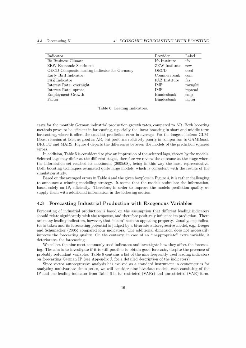
We collect the nine most commonly used indicators and investigate how they affect the forecast-ing. The aim is to investigate if it is still possible to obtain good forecasts, despite the presence ofprobably redundant variables. Table 6 contains a list of the nine frequently used leading indicatorson forecasting German IP (see Appendix A for a detailed description of the indicators).

Since vector autoregressive analysis has evolved as a standard instrument in econometrics foranalysing multivariate times series, we will consider nine bivariate models, each consisting of theIP and one leading indicator from Table 6 in its restricted (VARr) and unrestricted (VAR) form.

16

4.3 Forecasting II 4 ECONOMIC FORECASTING WITH BOOSTING

Indicator H VAR VARr GLMBoost GAMBoost BRUTO MARS

ifo 1 0.1101O 0.0914O 0.0647N 0.0675N 0.0845O 0.0892N6 0.1191O 0.1291O 0.0808N 0.0826N 0.1029N 0.0899O

12 0.0947N 0.1215O 0.1220N 0.1093N 0.1168O 0.1169O

zew 1 0.0742O 0.0724O 0.0643N 0.0754O 0.0766O 0.0826N6 0.1116O 0.1058O 0.0808N 0.0855O 0.1157O 0.0893O

12 0.0984N 0.1151N 0.1220N 0.1076N 0.1155N 0.1164O

oecd 1 0.0697O 0.0697O 0.0650O 0.0727O 0.0557N 0.1041O6 0.1055O 0.1058O 0.0808N 0.0852O 0.1245O 0.0829N

12 0.1588O 0.1141N 0.1220N 0.1100O 0.1117N 0.1188O

com 1 0.0862O 0.0840O 0.0704O 0.0751O 0.0789O 0.0764N6 0.0981N 0.0813N 0.0803N 0.0850O 0.1093O 0.0909O

12 0.1546O 0.1163N 0.1226N 0.1093N 0.1064N 0.1069O

faz 1 0.0698O 0.0655N 0.0648N 0.0737O 0.0830O 0.0916N6 0.3062O 0.3203O 0.0808N 0.0848N 0.1642O 0.0895O

12 0.2156O 0.1218O 0.1220N 0.1093N 0.1389O 0.1047O

rovnght 1 0.0604N 0.0605N 0.0648N 0.0731O 0.0717O 0.0910N6 0.0958O 0.1054O 0.0808N 0.0853O 0.1111O 0.0895O

12 0.1015N 0.1151N 0.1220N 0.1093N 0.1163O 0.1017O

rspread 1 0.0648N 0.0581N 0.0634N 0.0701O 0.0742O 0.0927O6 0.1010O 0.1058O 0.0808N 0.0848O 0.1005N 0.0890N

12 0.1049N 0.115N 0.1219N 0.1093N 0.1038N 0.1052O

emp 1 0.0671O 0.0792O 0.0632N 0.0696N 0.0704N 0.0916N6 0.0976N 0.1004N 0.1036O 0.0946O 0.1396O 0.0919O

12 0.1090N 0.1250O 0.1356O 0.1190O 0.1361O 0.1082O

factor 1 0.0514N 0.0519N 0.0550N 0.0684N 0.0558N 0.0948O6 0.0988N 0.1004N 0.0861O 0.0823N 0.0990O 0.0914O

12 0.1088N 0.1077N 0.1209O 0.1161O 0.1034N 0.1147O

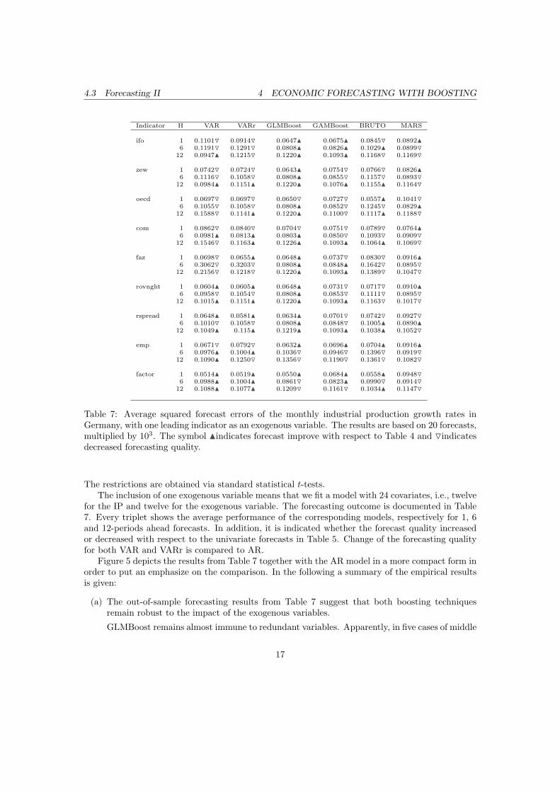
Table 7: Average squared forecast errors of the monthly industrial production growth rates inGermany, with one leading indicator as an exogenous variable. The results are based on 20 forecasts,multiplied by 103. The symbol Nindicates forecast improve with respect to Table 4 and Oindicatesdecreased forecasting quality.

The restrictions are obtained via standard statistical t-tests.The inclusion of one exogenous variable means that we fit a model with 24 covariates, i.e., twelve

for the IP and twelve for the exogenous variable. The forecasting outcome is documented in Table7. Every triplet shows the average performance of the corresponding models, respectively for 1, 6and 12-periods ahead forecasts. In addition, it is indicated whether the forecast quality increasedor decreased with respect to the univariate forecasts in Table 5. Change of the forecasting qualityfor both VAR and VARr is compared to AR.

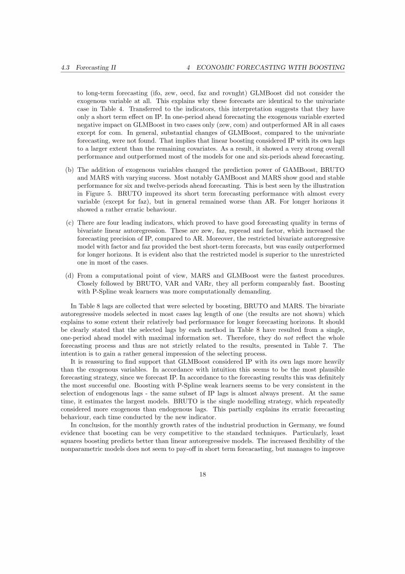
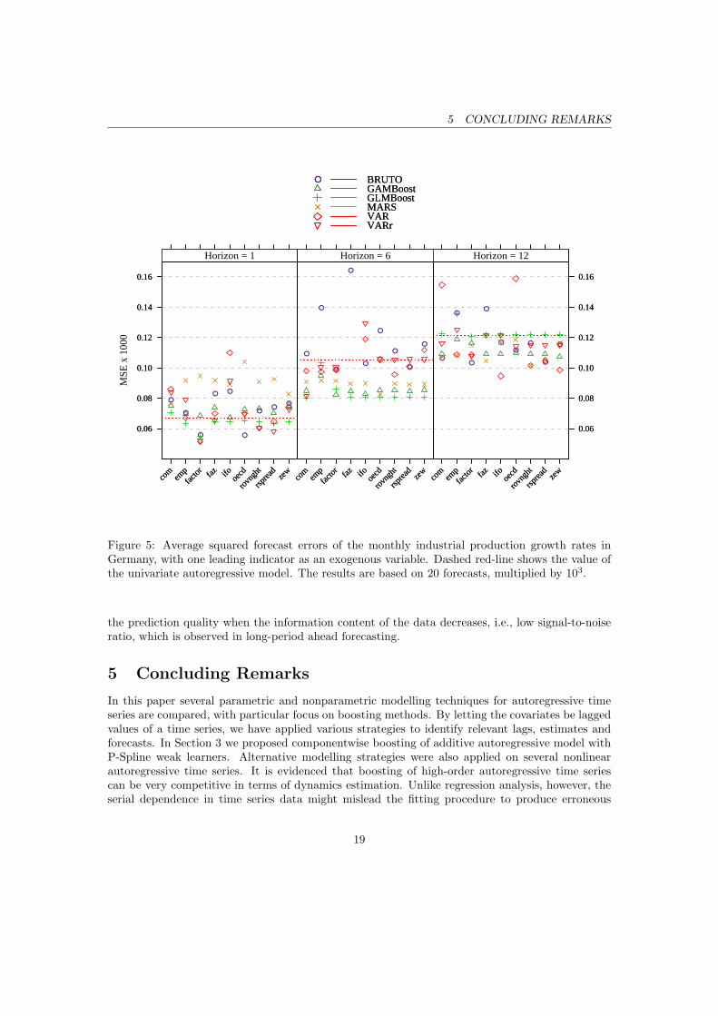
Figure 5 depicts the results from Table 7 together with the AR model in a more compact form inorder to put an emphasize on the comparison. In the following a summary of the empirical resultsis given:

(a) The out-of-sample forecasting results from Table 7 suggest that both boosting techniquesremain robust to the impact of the exogenous variables.

GLMBoost remains almost immune to redundant variables. Apparently, in five cases of middle

17

4.3 Forecasting II 4 ECONOMIC FORECASTING WITH BOOSTING

to long-term forecasting (ifo, zew, oecd, faz and rovnght) GLMBoost did not consider theexogenous variable at all. This explains why these forecasts are identical to the univariatecase in Table 4. Transferred to the indicators, this interpretation suggests that they haveonly a short term effect on IP. In one-period ahead forecasting the exogenous variable exertednegative impact on GLMBoost in two cases only (zew, com) and outperformed AR in all casesexcept for com. In general, substantial changes of GLMBoost, compared to the univariateforecasting, were not found. That implies that linear boosting considered IP with its own lagsto a larger extent than the remaining covariates. As a result, it showed a very strong overallperformance and outperformed most of the models for one and six-periods ahead forecasting.

(b) The addition of exogenous variables changed the prediction power of GAMBoost, BRUTOand MARS with varying success. Most notably GAMBoost and MARS show good and stableperformance for six and twelve-periods ahead forecasting. This is best seen by the illustrationin Figure 5. BRUTO improved its short term forecasting performance with almost everyvariable (except for faz), but in general remained worse than AR. For longer horizons itshowed a rather erratic behaviour.

(c) There are four leading indicators, which proved to have good forecasting quality in terms ofbivariate linear autoregression. These are zew, faz, rspread and factor, which increased theforecasting precision of IP, compared to AR. Moreover, the restricted bivariate autoregressivemodel with factor and faz provided the best short-term forecasts, but was easily outperformedfor longer horizons. It is evident also that the restricted model is superior to the unrestrictedone in most of the cases.

(d) From a computational point of view, MARS and GLMBoost were the fastest procedures.Closely followed by BRUTO, VAR and VARr, they all perform comparably fast. Boostingwith P-Spline weak learners was more computationally demanding.

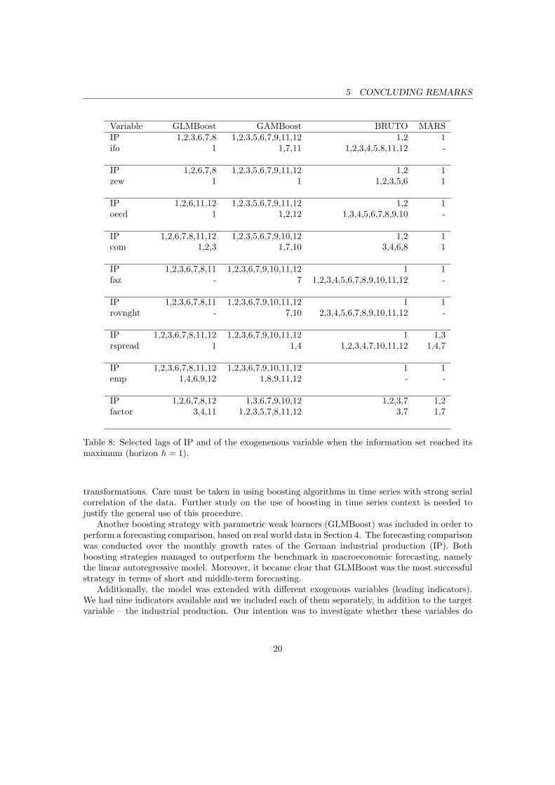
In Table 8 lags are collected that were selected by boosting, BRUTO and MARS. The bivariateautoregressive models selected in most cases lag length of one (the results are not shown) whichexplains to some extent their relatively bad performance for longer forecasting horizons. It shouldbe clearly stated that the selected lags by each method in Table 8 have resulted from a single,one-period ahead model with maximal information set. Therefore, they do not reflect the wholeforecasting process and thus are not strictly related to the results, presented in Table 7. Theintention is to gain a rather general impression of the selecting process.

It is reassuring to find support that GLMBoost considered IP with its own lags more heavilythan the exogenous variables. In accordance with intuition this seems to be the most plausibleforecasting strategy, since we forecast IP. In accordance to the forecasting results this was definitelythe most successful one. Boosting with P-Spline weak learners seems to be very consistent in theselection of endogenous lags - the same subset of IP lags is almost always present. At the sametime, it estimates the largest models. BRUTO is the single modelling strategy, which repeatedlyconsidered more exogenous than endogenous lags. This partially explains its erratic forecastingbehaviour, each time conducted by the new indicator.

In conclusion, for the monthly growth rates of the industrial production in Germany, we foundevidence that boosting can be very competitive to the standard techniques. Particularly, leastsquares boosting predicts better than linear autoregressive models. The increased flexibility of thenonparametric models does not seem to pay-off in short term foreacasting, but manages to improve

18

5 CONCLUDING REMARKSM

SE

x 1

000

0.06

0.08

0.10

0.12

0.14

0.16

com

empfa

ctor

faz ifo oe

cd

rovn

ght

rspr

ead

zew

●

●

●

●●

●●

●

●

Horizon = 1

com

empfa

ctor

faz ifo oe

cd

rovn

ght

rspr

ead

zew

●

●

●

●

●

●

●

●

●

Horizon = 6

com

empfa

ctor

faz ifo oe

cd

rovn

ght

rspr

ead

zew

0.06

0.08

0.10

0.12

0.14

0.16

● ●●

●

●

●

●

●

●

Horizon = 12

● BRUTOGAMBoostGLMBoostMARSVARVARr

0.06

0.08

0.10

0.12

0.14

0.16

com

empfa

ctor

faz ifo oe

cd

rovn

ght

rspr

ead

zew

Horizon = 1

com

empfa

ctor

faz ifo oe

cd

rovn

ght

rspr

ead

zew

Horizon = 6

com

empfa

ctor

faz ifo oe

cd

rovn

ght

rspr

ead

zew

0.06

0.08

0.10

0.12

0.14

0.16

Horizon = 12

● BRUTOGAMBoostGLMBoostMARSVARVARr

Figure 5: Average squared forecast errors of the monthly industrial production growth rates inGermany, with one leading indicator as an exogenous variable. Dashed red-line shows the value ofthe univariate autoregressive model. The results are based on 20 forecasts, multiplied by 103.

the prediction quality when the information content of the data decreases, i.e., low signal-to-noiseratio, which is observed in long-period ahead forecasting.

5 Concluding Remarks

In this paper several parametric and nonparametric modelling techniques for autoregressive timeseries are compared, with particular focus on boosting methods. By letting the covariates be laggedvalues of a time series, we have applied various strategies to identify relevant lags, estimates andforecasts. In Section 3 we proposed componentwise boosting of additive autoregressive model withP-Spline weak learners. Alternative modelling strategies were also applied on several nonlinearautoregressive time series. It is evidenced that boosting of high-order autoregressive time seriescan be very competitive in terms of dynamics estimation. Unlike regression analysis, however, theserial dependence in time series data might mislead the fitting procedure to produce erroneous

19

5 CONCLUDING REMARKS

Variable GLMBoost GAMBoost BRUTO MARSIP 1,2,3,6,7,8 1,2,3,5,6,7,9,11,12 1,2 1ifo 1 1,7,11 1,2,3,4,5,8,11,12 -

IP 1,2,6,7,8 1,2,3,5,6,7,9,11,12 1,2 1zew 1 1 1,2,3,5,6 1

IP 1,2,6,11,12 1,2,3,5,6,7,9,11,12 1,2 1oecd 1 1,2,12 1,3,4,5,6,7,8,9,10 -

IP 1,2,6,7,8,11,12 1,2,3,5,6,7,9,10,12 1,2 1com 1,2,3 1,7,10 3,4,6,8 1

IP 1,2,3,6,7,8,11 1,2,3,6,7,9,10,11,12 1 1faz - 7 1,2,3,4,5,6,7,8,9,10,11,12 -

IP 1,2,3,6,7,8,11 1,2,3,6,7,9,10,11,12 1 1rovnght - 7,10 2,3,4,5,6,7,8,9,10,11,12 -

IP 1,2,3,6,7,8,11,12 1,2,3,6,7,9,10,11,12 1 1,3rspread 1 1,4 1,2,3,4,7,10,11,12 1,4,7

IP 1,2,3,6,7,8,11,12 1,2,3,6,7,9,10,11,12 1 1emp 1,4,6,9,12 1,8,9,11,12 - -

IP 1,2,6,7,8,12 1,3,6,7,9,10,12 1,2,3,7 1,2factor 3,4,11 1,2,3,5,7,8,11,12 3,7 1,7

Table 8: Selected lags of IP and of the exogenenous variable when the information set reached itsmaximum (horizon h = 1).

transformations. Care must be taken in using boosting algorithms in time series with strong serialcorrelation of the data. Further study on the use of boosting in time series context is needed tojustify the general use of this procedure.

Another boosting strategy with parametric weak learners (GLMBoost) was included in order toperform a forecasting comparison, based on real world data in Section 4. The forecasting comparisonwas conducted over the monthly growth rates of the German industrial production (IP). Bothboosting strategies managed to outperform the benchmark in macroeconomic forecasting, namelythe linear autoregressive model. Moreover, it became clear that GLMBoost was the most successfulstrategy in terms of short and middle-term forecasting.

Additionally, the model was extended with different exogenous variables (leading indicators).We had nine indicators available and we included each of them separately, in addition to the targetvariable – the industrial production. Our intention was to investigate whether these variables do

20

5 CONCLUDING REMARKS

indeed improve the forecasting quality of the industrial production and how boosting handles thesehigh-dimensional models. Thus, having formed nine high-dimensional models, we forecasted againthe monthly growth rates of IP. Linear bivariate autoregressive models were also considered asstandard tools for forecasting. Our approach using componentwise linear and additive models in afunction gradient descent algorithm improves upon likelihood based boosting applied to nonlinearautoregressive times series models (Shafik and Tutz, 2009) in two respects. First, more flexibleregression functions can be estimated using our approach (linear effects, decompositions of linearand smooth effects or interaction effects (Kneib et al., 2009)). Second, further research establishedalternative characteristics of the response to be regressed on lags or exogenous variables, mostimportantly quantile regression approaches implemented via componentwise functional gradientdescent (Fenske et al., 2009).

The variables’ impact on the forecasting quality had debatable success, since in many of the casestheir inclusion worsened the forecasting performance, compared to the univariate case. GLMBoost,on the other hand, was almost immune to redundant variables by performing at least as good asin the univariate case. In one-period ahead forecasting, GAMBoost was affected by the additionalvariables rather strongly, which was counterproductive for its overall performance, when comparedto the univariate case. The increased flexibility of GAMBoost was useful, however, in middleand long term forecasting, where the information content of the data is very low, i.e. it has lowsignal-to-noise ratio.

Another crucial topic for further development addresses the multivariate generalization of boost-ing. The first steps toward high dimensionality in the response were made by Lutz et al. (2007), whoprovided theoretical grounds and empirical evidence for its usability. Applying this approach wouldopen new perspective for forecasting with boosting, based on iterative forecasts of multivariatemodels.

Computational Details

All data analyses presented in this paper have been carried out using the R system for statisticalcomputation (Team, 2009), version 2.9.2. There are several implementations of boosting techniques,available as add-on packages for R. Package mboost (Hothorn et al., 2009) provides an implemen-tation for fitting generalized linear models, as well as additive gradient based boosting.

Our simulations were carried out with mboost. As weak learner we use P-Splines, provided bythe function bbs() and subsequently fitted by the gamboost() function.

We use 20 knots (knots = 20), we set M = 500 (mstop = 500) as an upper bound for boostingand set the degrees of freedom to 3.5, i.e. degree = 3.5. The optimal number of steps is evaluatedvia the corrected AIC criterion provided by the AIC() function. For all other options we use thedefault values.

Further on, we consider the method proposed by Huang and Yang (2004), which uses splinefitting with BIC. Their novel approach was manually implemented since it is currently not availableas an extension package for R or in any other statistical software.

The implementation was carried out by the package mgcv (Wood, 2006, 2009) with unpenalizedcubic splines. The maximum number of candidate variables was equalled to the maximal numberof lags.

An implementation of BRUTO can be found in package mda (Hastie, Tibshirani, Leisch, Hornikand Ripley., 2009). The corresponding function bruto() has a tuning parameter cost which spec-ifies the cost per degree-of-freedom change. It was empirically investigated by Huang and Yang

21

5 CONCLUDING REMARKS

(2004) that a value of log(n) provides much better results than the default value of two, where nindicates the sample size. Therefore, in our application cost was set to log(n) too.

An implementation of MARS is available in package mda and the corresponding function ismars(). It has a tuning parameter which charges a cost per basis function, denoted by penalty.This tuning parameter was also set to log(n).

The estimation of AR is carried out via the ar() function in package stats with AIC criterion.The package vars (Pfaff, 2008) offers “standard” tools in the context of purely vector autoregressivemodels. We use a modified version of its function VAR in order to consider direct forecasting. Thecorresponding information criterion is AIC.

22

A THE CHOICE OF LEADING INDICATORS

APPENDIX

A The Choice of Leading Indicators

In Section 4 nine leading indicators were chosen. These are summarized as follows.The Ifo Business Climate Index is based on about 7,000 monthly survey responses of firms in

manufacturing, construction, wholesaling and retailing. The firms are asked to give their assess-ments of the current business situation and their expectations for the next six months. The balancevalue of the current business situation is the difference of the percentages of the ”good” and respec-tively ”poor” responses, the balance value of the expectations is the difference of the percentages ofthe ”more favourable” and ”more unfavourable” responses. The business climate is a transformedmean of the balances of the business situation and the expectations. For further information seeGoldrian (2007).

The ZEW Indicator of Economic Sentiment is published monthly. Up to 350 financial expertstake part in the survey. The indicator reflects the difference between the share of analysts thatare optimistic and the share of analysts that are pessimistic with regard to the expected economicdevelopment in Germany within six months (see Hufner and Schroder, 2002).

The FAZ indicator (Frankfurter Allgemeine Zeitung) pools survey data and macroeconomic timeseries. It consists of the Ifo index (0.13), new orders in manufacturing industries (0.56), the realeffective exchange rate of the Euro (0.06), the interest rate spread (0.08), the stock market indexDAX (0.01), the number of job vacancies (0.05) and lagged industrial production (0.11). The Ifoindex, orders in manufacturing and the number of job vacancies enter the indicator equation inlevels, while the other variables are measured in first differences.

The Early Bird indicator, compiled by Commerzbank, also pools different time series and stressesthe importance of international business cycles for the German economy. Its components are thereal effective exchange rate of the Euro (0.35), the short-term real interest rate (0.4), defined asthe difference between the short-term nominal rate and core inflation, and the purchasing managerindex of U.S. manufactures (0.25).

The OECD composite leading indicator is delivered by using a modified version of the Phase-Average Trend method (PAT) developed by the US National Bureau of Economic Research (NBER).The indicator is compiled by combining de-trended component series in either their seasonallyadjusted or raw form. The component series are selected based on various criteria such as economicsignificance, cyclical behaviour, data quality, timeliness and availability. For Germany the followingtime series are compiled: Orders inflow or demand: tendency (manufacturing) (% balance), IfoBusiness climate indicator (manufacturing) (% balance), Spread of interest rates (% annual rate),Total new orders (manufacturing), Finished goods stocks: level (manufacturing) (% balance) andExport order books: level (manufacturing) (% balance).

Financial indicators, such as overnight interbank interest rate an interest spread, are used aspossible predictors as well. Stock and Watson (2003) have conducted a thorough case study fordifferent OECD countries by forecasting Gross Domestic Product (GDP), Inflation and Industrialproduction. The information on the growth of the employment in Germany has been taken fromtheir paper.

Finally, a factor indicator obtained from a large data set from Germany, is included. The dataset contains the German quarterly GDP and 111 monthly indicators from 1992 to 2006.2

2The estimated factor was provided by Christian Schumacher and is based on Marcellino and Schumacher (2007).

23

REFERENCES REFERENCES

References

Benner, J. and Meier, C. (2004). Prognosegute alternativer Fruhindikatoren fur die Konjunktur inDeutschland, Jahrbucher fur Nationalokonomie und Statistik 224(6): 637–652.

Buhlmann, P. (2006). Boosting for high-dimensional linear models, The Annals of Statistics34(2): 559–583.

Buhlmann, P. and Hothorn, T. (2007). Boosting algorithms: Regularization, prediction and modelfitting, Statistical Science 22(4): 477–505.

Buhlmann, P. and Yu, B. (2003). Boosting with the l2 loss: Regression and classification, Journalof the American Statistical Association 98(462): 324–339.

Chen, R. and Tsay, R. (1993). Nonlinear additive ARX models, Journal of the American StatisticalAssociation 88(423): 955–967.

Chevillon, G. and Hendry, D. (2005). Non-parametric direct multi-step estimation for forecastingeconomic processes, International Journal of Forecasting 21(2): 201–218.

Claveria, O., Pons, E. and Ramos, R. (2007). Business and consumer expectations and macroeco-nomic forecasts, International Journal of Forecasting 23(1): 47–69.

Clements, M., Franses, P. and Swanson, N. (2004). Forecasting economic and financial time-serieswith non-linear models, International Journal of Forecasting 20(2): 169–183.

Dreger, C. and Schumacher, C. (2005). Out-of-sample performance of leading indicators for theGerman business cycle. Single vs combined forecasts, Journal of Business Cycle Measurementand Analysis 2(1): 71–88.

Eilers, P. and Marx, B. (1996). Flexible smoothing with B-splines and penalties, Statistical Science11(2): 89–102.

Elliot, G. and Timmermann, A. (2008). Economic forecasting, Journal of Economic Literature66(1): 3–56.

Fenske, N., Kneib, T. and Hothorn, T. (2009). Identifying risk factors for severe childhood mal-nutrition by boosting additive quantile regression., Technical Report 52, Institut fur Statistik,Ludwig-Maximilians-Universitat Munchen.URL: http://epub.ub.uni-muenchen.de/10510/

Freund, Y. and Schapire, R. (1996). Experiments with a new boosting algorithm, Proceedings of theThirteenth International Conference on Machine Learning, Morgan Kaufmann Publishers Inc.,San Francisco, CA, pp. 148–156.

Friedman, J. (1991). Multivariate adaptive regression splines, The Annals of Statistics 19(1): 1–67.

Friedman, J. (2001). Greedy function approximation: A gradient boosting machine, The Annals ofStatistics 29(5): 1189–1232.

Hamilton, J. (1994). Time Series Analysis, Princeton University Press.

24

REFERENCES REFERENCES

Hastie, T. and Tibshirani, R. (1990). Generalized Additive Models, Chapman & Hall/CRC.

Hastie, T., Tibshirani, R. and Friedman, J. (2001). The Elements of Statistical Learning: DataMining, Inference, and Prediction, Springer.

Hastie, T., Tibshirani, R. and Friedman, J. (2009). The Elements of Statistical Learning: DataMining, Inference, and Prediction, 2nd edn, Springer.

Hastie, T., Tibshirani, R., Leisch, F., Hornik, K. and Ripley., B. D. (2009). mda: Mixture andFlexible Discriminant Analysis. R package version 0.3-4.

Hothorn, T., Buhlmann, P., Kneib, T. and Schmid, M. (2009). mboost: Model-Based Boosting, Rpackage, version 1.0-7.URL: http://CRAN.R-project.org/package=mboost

Huang, J. and Yang, L. (2004). Identification of non-linear additive autoregressive models, Journalof the Royal Statistical Society Series B(Statistical Methodology) 66(2): 463–477.

Hufner, F. and Schroder, M. (2002). Prognosegehalt von ifo-Geschaftserwartungen und ZEW-Konjunkturerwartungen: Ein okonometrischer Vergleich, Jahrbucher fur Nationalokonomie undStatistik 222(3): 316–336.

Hurvich, C. M., Simonoff, J. S. and Tsai, C.-L. (1998). Smoothing parameter selection in nonpara-metric regression using an improved Akaike information criterion, Journal of the Royal Statistis-tical Society, Series B 60: 271–293.

Hyndman, R. and Koehler, A. (2006). Another look at measures of forecast accuracy, InternationalJournal of Forecasting 22(4): 679–688.

Kneib, T., Hothorn, T. and Tutz, G. (2009). Variable selection and model choice in geoadditiveregression models, Biometrics 65: 626–634.

Lewis, P. and Stevens, J. (1991). Nonlinear modeling of time series using multivariate adaptiveregression splines (MARS)., Journal of the American Statistical Association 86(416): 864–877.

Lutkepohl, H. (1991). Introduction to Multiple Time Series Analysis, Springer, Berlin.

Lutkepohl, H. (2006). New Introduction to Multiple Time Series Analysis, Springer.

Lutz, R., Kalisch, M. and Buhlmann, P. (2007). Robustified l2 boosting, Technical report, Seminarfur Statistik ETH Zurich.

Marcellino, M. and Schumacher, C. (2007). Factor nowcasting of German GDP with ragged-edgedata. A model comparison using MIDAS projections, Technical report, Bundesbank DiscussionPaper, Series 1, 34/2007.

Marcellino, M., Stock, J. and Watson, M. (2006). A comparison of direct and iterated multistep ARmethods for forecasting macroeconomic time series, Journal of Econometrics 135(1-2): 499–526.

Meinshausen, N. and Buhlmann, P. (2010). Stability selection, Journal of the Royal StatisticalSociety, Series B 72(4): 1–32.

25

REFERENCES REFERENCES

Pfaff, B. (2008). VAR, SVAR and SVEC models: Implementation within R package vars, Journalof Statistical Software 27(4).URL: http://www.jstatsoft.org/v27/i04/

Robinzonov, N. and Wohlrabe, K. (2010). Freedom of choice in macroeconomic forecasting, CESifoEconomic Studies 56(1).

Schmid, M. and Hothorn, T. (2008). Boosting additive models using component-wise P-splines,Computational Statistics & Data Analysis 53(2): 298–311.

Shafik, N. and Tutz, G. (2009). Boosting nonlinear additive autoregressive time series, Computa-tional Statistics & Data Analysis 53(7): 2453–2464.

Stock, J. and Watson, M. (2003). Forecasting output and inflation: The role of asset prices, Journalof Economic Literature 41(3): 788–829.

Team, R. D. C. (2009). R: A Language and Environment for Statistical Computing, R Foundationfor Statistical Computing, Vienna, Austria. ISBN 3-900051-07-0.URL: http://www.R-project.org

Terasvirta, T., van Dijk, D. and Medeiros, M. (2005). Linear models, smooth transition autore-gressions, and neural networks for forecasting macroeconomic time series: A reexamination,International Journal of Forecasting 21(4): 755–774.

Tschernig, R. and Yang, L. (2000). Nonparametric lag selection for time series, Journal of TimeSeries Analysis 21(4): 457–487.

Wood, S. (2006). Generalized Additive Models: An Introduction with R, Chapman & Hall/CRC.

Wood, S. (2009). mgcv: GAMs with GCV smoothness estimation and GAMMs by REML/PQL, Rpackage, version 1.4-1.1.

26