Embed Size (px)
Citation preview
1
Blind (Uninformed) Search
(Where we systematically explore alternatives)
R&N: Chap. 3, Sect. 3.3–5
Sunday, February 26, 12
2
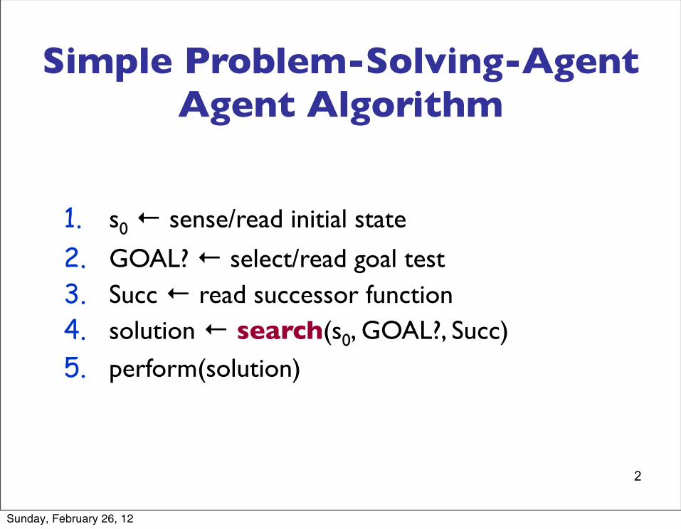
Simple Problem-Solving-Agent Agent Algorithm
1. s0 ← sense/read initial state
2. GOAL? ← select/read goal test3. Succ ← read successor function4. solution ← search(s0, GOAL?, Succ) 5. perform(solution)
Sunday, February 26, 12
3
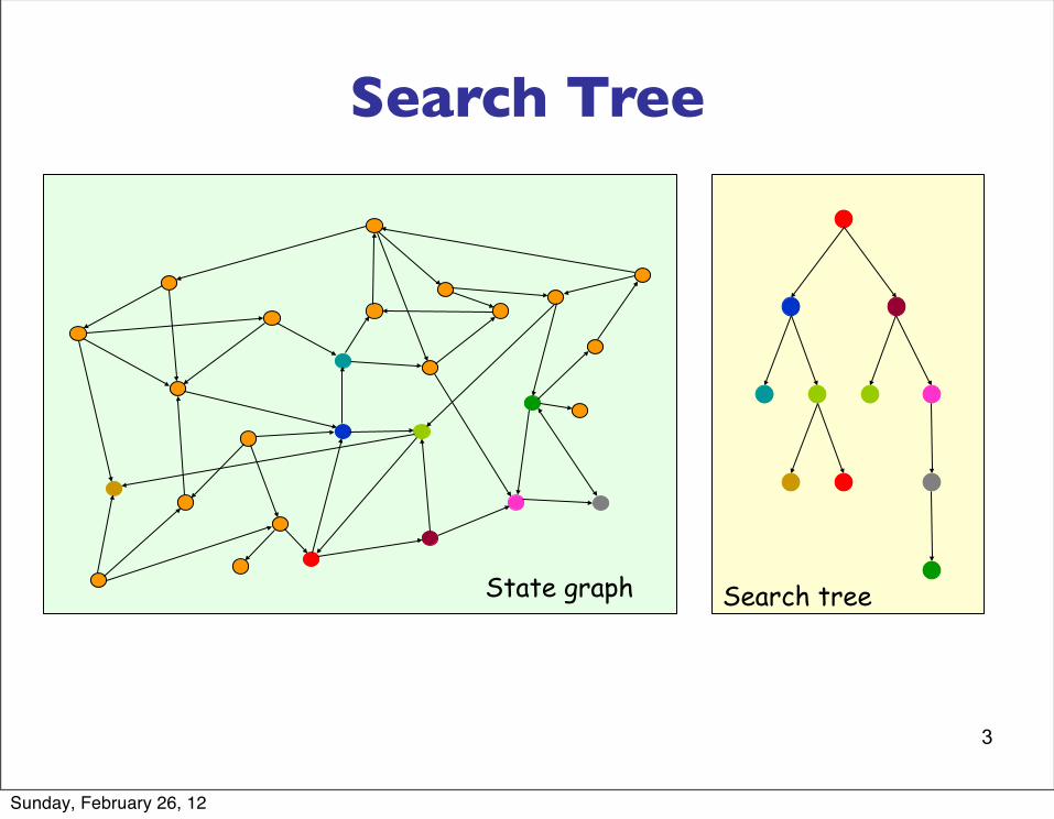
Search Tree
Search treeState graph
Sunday, February 26, 12
3
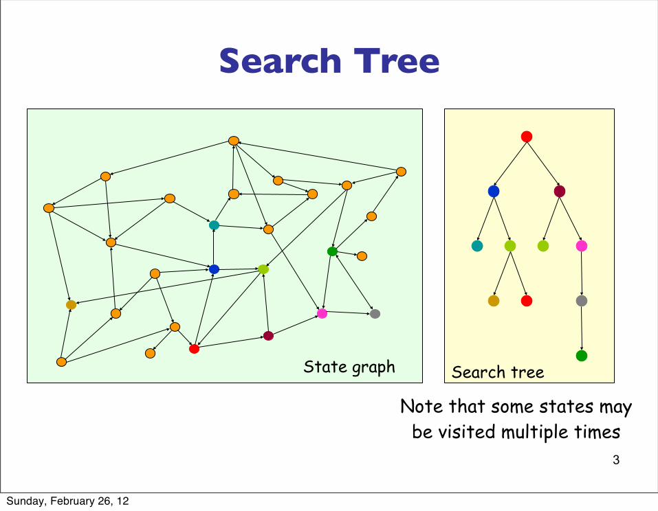
Search Tree
Search tree
Note that some states may be visited multiple times
State graph
Sunday, February 26, 12
4
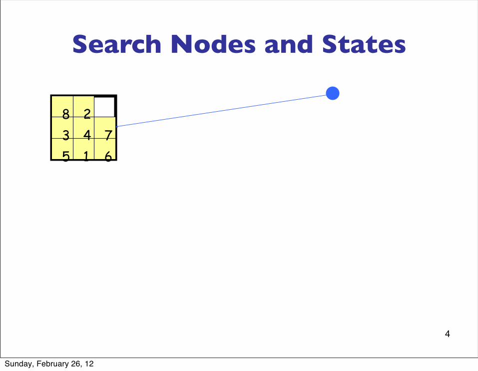
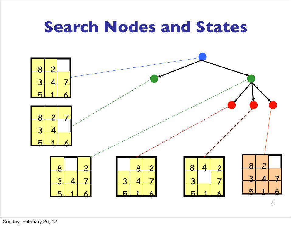
Search Nodes and States
1
23 45 6
78
Sunday, February 26, 12
4
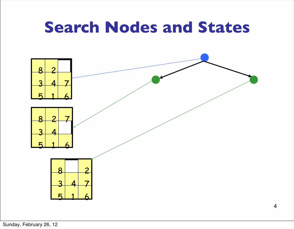
Search Nodes and States
1
23 45 6
78
1
23 45 6
78
1
23 45 6
78
Sunday, February 26, 12
4
Search Nodes and States
1
23 45 6
78
1
23 45 6
78
1
23 45 6
78
135 6
8
13
4
5 67
824 7
2
1
23 45 6
78
Sunday, February 26, 12
5
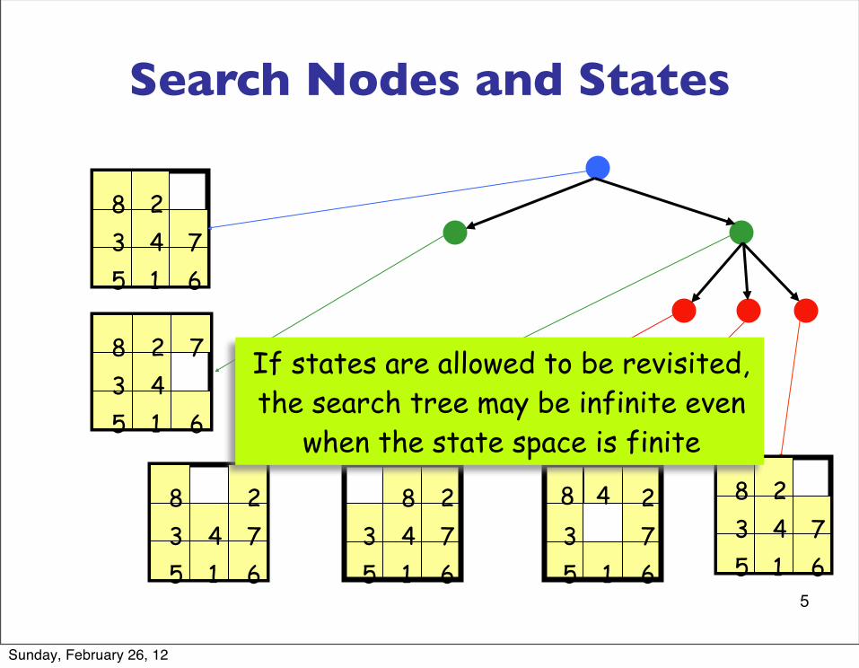
Search Nodes and States
1
23 45 6
78
1
23 45 6
78
1
23 45 6
78
135 6
8
13
4
5 67
824 7
2
1
23 45 6
78
If states are allowed to be revisited,the search tree may be infinite even
when the state space is finite
Sunday, February 26, 12
6
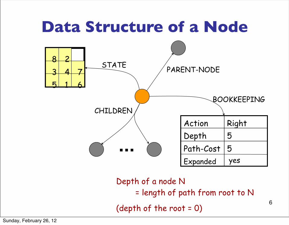
Data Structure of a Node
PARENT-NODE
1
23 45 6
78
STATE
Depth of a node N = length of path from root to N
(depth of the root = 0)
BOOKKEEPING
5Path-Cost5DepthRightAction
Expanded yes...
CHILDREN
Sunday, February 26, 12
8
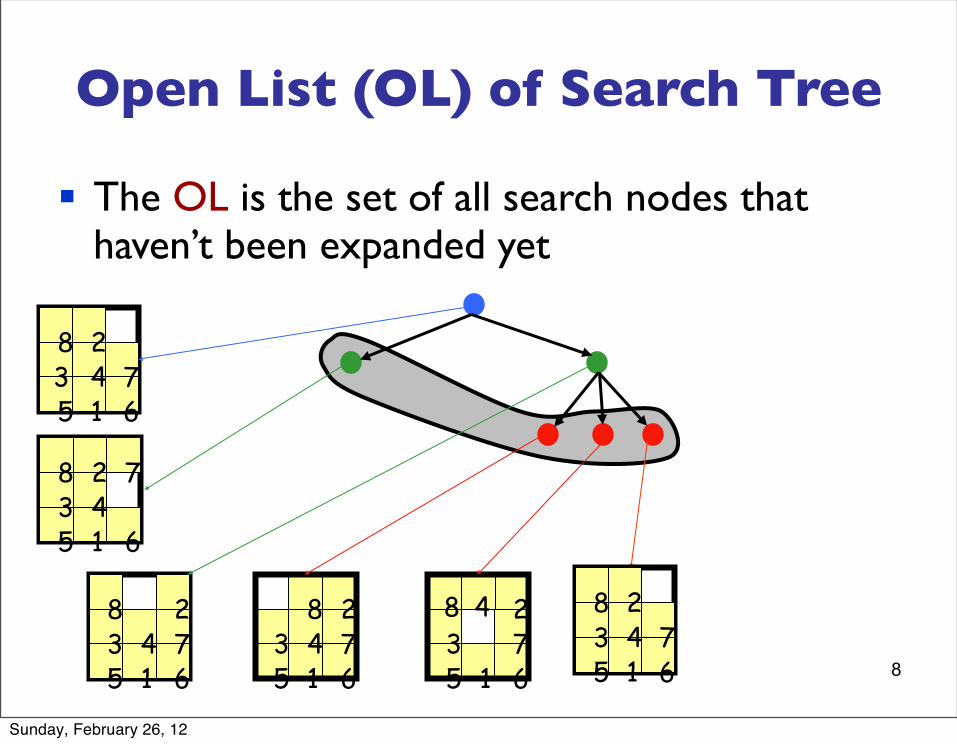
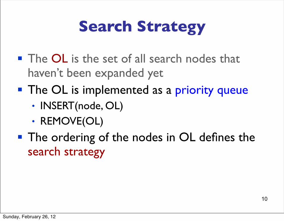
Open List (OL) of Search Tree
§ The OL is the set of all search nodes that haven’t been expanded yet
1
23 45 6
78
1
23 45 6
78
1
23 45 6
78
135 6
8
13
4
5 67
824 7
2
1
23 45 6
78
Sunday, February 26, 12
10
Search Strategy
§ The OL is the set of all search nodes that haven’t been expanded yet
§ The OL is implemented as a priority queue• INSERT(node, OL)
• REMOVE(OL)
§ The ordering of the nodes in OL defines the search strategy
Sunday, February 26, 12
11
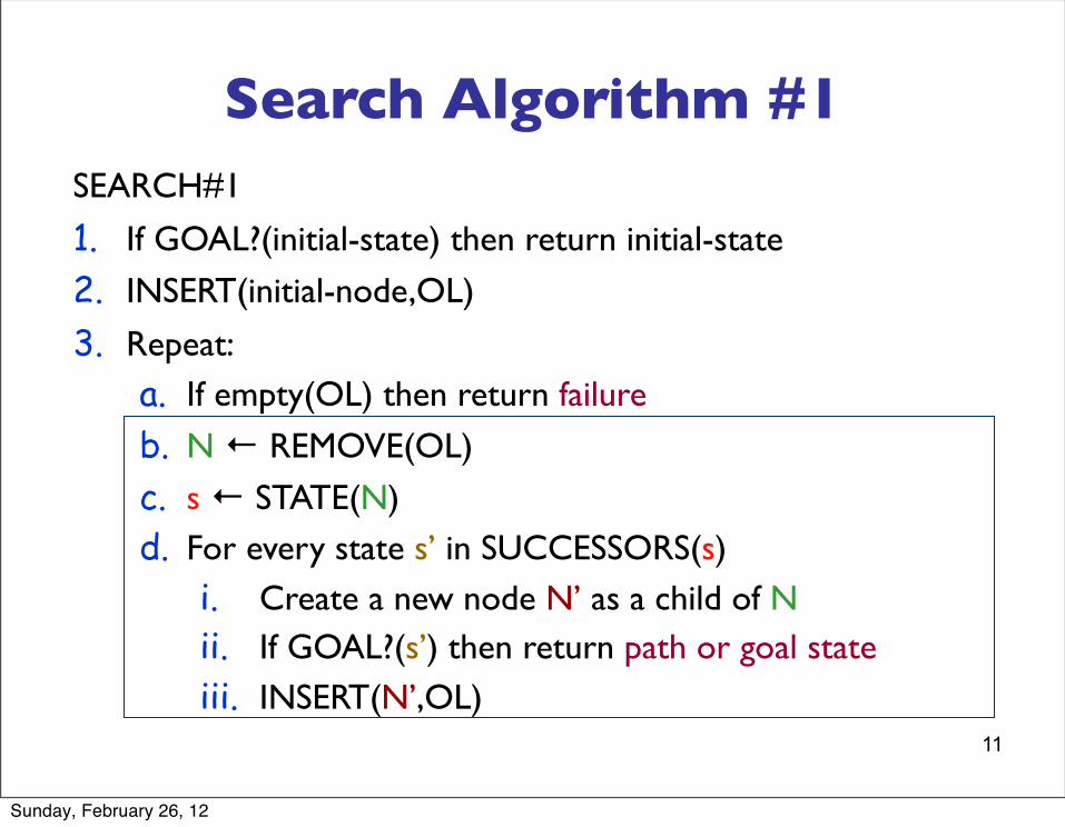
Search Algorithm #1SEARCH#1
1. If GOAL?(initial-state) then return initial-state
2. INSERT(initial-node,OL)
3. Repeat:a. If empty(OL) then return failure
b. N ← REMOVE(OL)
c. s ← STATE(N)d. For every state s’ in SUCCESSORS(s)
i. Create a new node N’ as a child of Nii. If GOAL?(s’) then return path or goal stateiii. INSERT(N’,OL)
Sunday, February 26, 12
12
Performance Measures
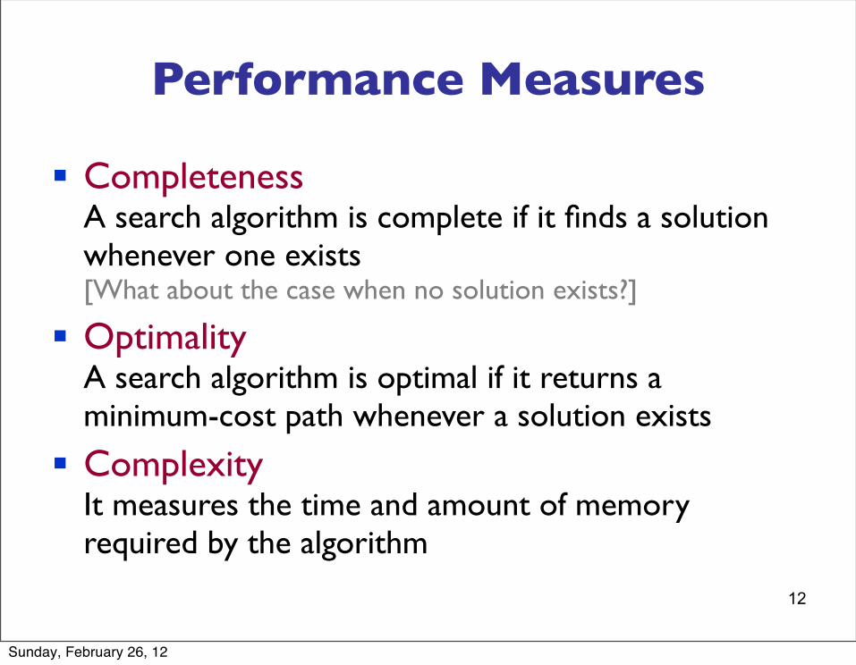
§ CompletenessA search algorithm is complete if it finds a solution whenever one exists[What about the case when no solution exists?]
§ OptimalityA search algorithm is optimal if it returns a minimum-cost path whenever a solution exists
§ ComplexityIt measures the time and amount of memory required by the algorithm
Sunday, February 26, 12
13
Blind vs. Heuristic Strategies
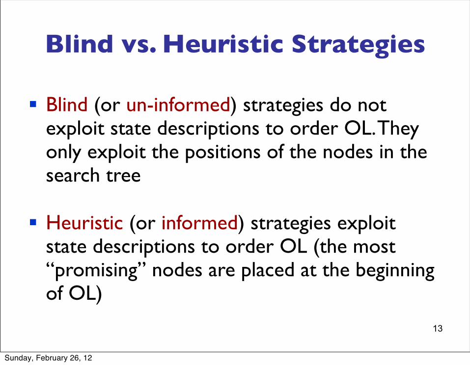
§ Blind (or un-informed) strategies do not exploit state descriptions to order OL. They only exploit the positions of the nodes in the search tree
§ Heuristic (or informed) strategies exploit state descriptions to order OL (the most “promising” nodes are placed at the beginning of OL)
Sunday, February 26, 12
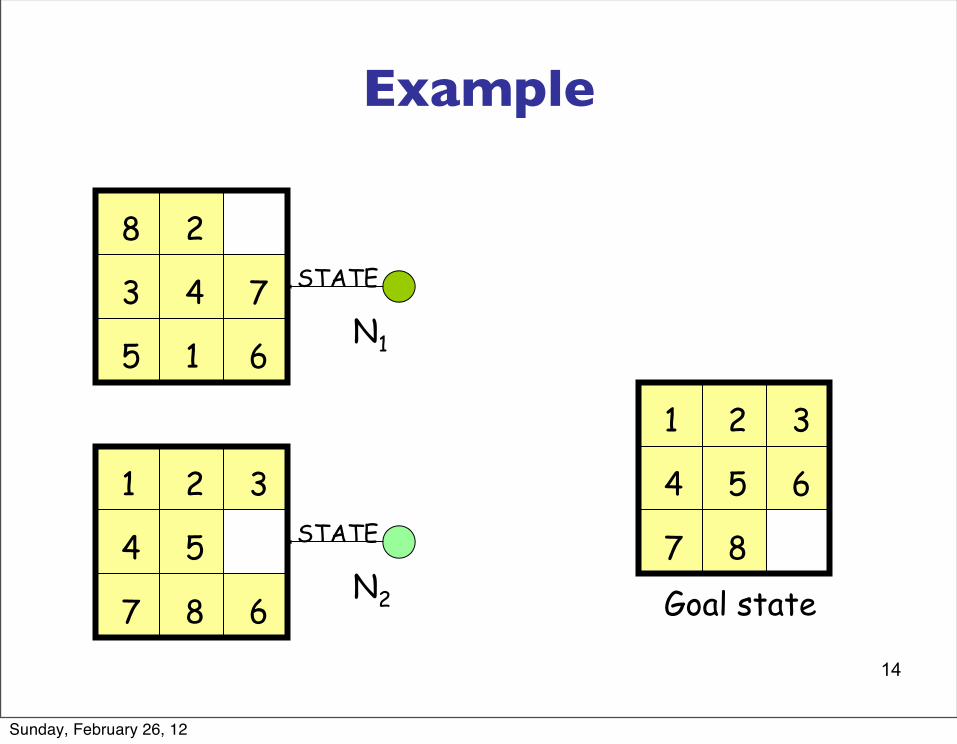
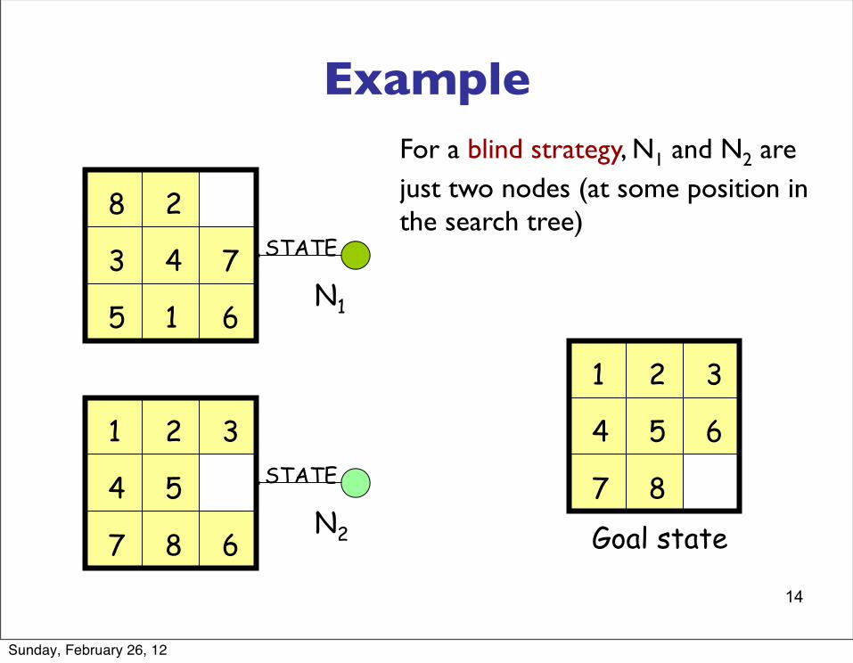
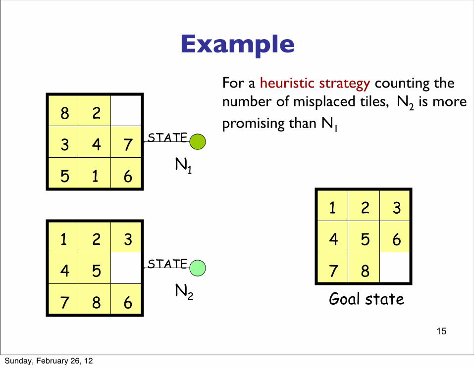
14
Example
Goal state
N1
N2
STATE
STATE
1
2
3 4
5 6
7
8
1 2 3
4 5
67 8
1 2 3
4 5 6
7 8
Sunday, February 26, 12
14
ExampleFor a blind strategy, N1 and N2 are just two nodes (at some position in the search tree)
Goal state
N1
N2
STATE
STATE
1
2
3 4
5 6
7
8
1 2 3
4 5
67 8
1 2 3
4 5 6
7 8
Sunday, February 26, 12
15
ExampleFor a heuristic strategy counting the number of misplaced tiles, N2 is more promising than N1
Goal state
N1
N2
STATE
STATE
1
2
3 4
5 6
7
8
1 2 3
4 5
67 8
1 2 3
4 5 6
7 8
Sunday, February 26, 12
16
Remark
§ Some search problems, such as the (n2-1)-puzzle, are NP-hard
§ One can’t expect to solve all instances of such problems in less than exponential time (in n)
§ One may still strive to solve each instance as efficiently as possible
This is the purpose of the search strategy
Sunday, February 26, 12
17
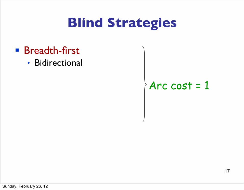
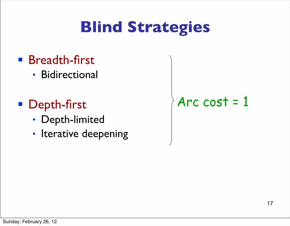
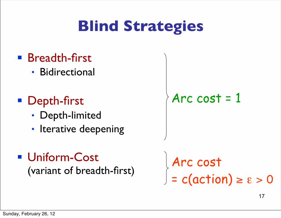
Blind Strategies
Sunday, February 26, 12
17
Blind Strategies
Arc cost = 1
Sunday, February 26, 12
17
Blind Strategies
§ Breadth-first• Bidirectional
Arc cost = 1
Sunday, February 26, 12
17
Blind Strategies
§ Breadth-first• Bidirectional
§ Depth-first• Depth-limited • Iterative deepening
Arc cost = 1
Sunday, February 26, 12
17
Blind Strategies
§ Breadth-first• Bidirectional
§ Depth-first• Depth-limited • Iterative deepening
§ Uniform-Cost(variant of breadth-first)
Arc cost = 1
Arc cost = c(action) ≥ ε > 0
Sunday, February 26, 12
18
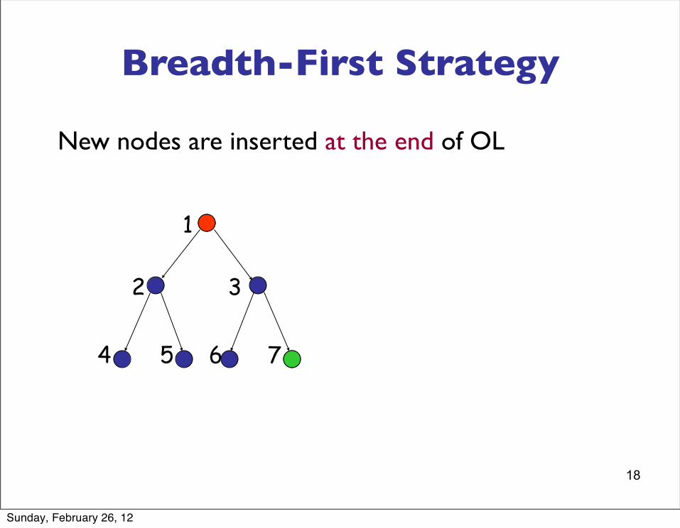
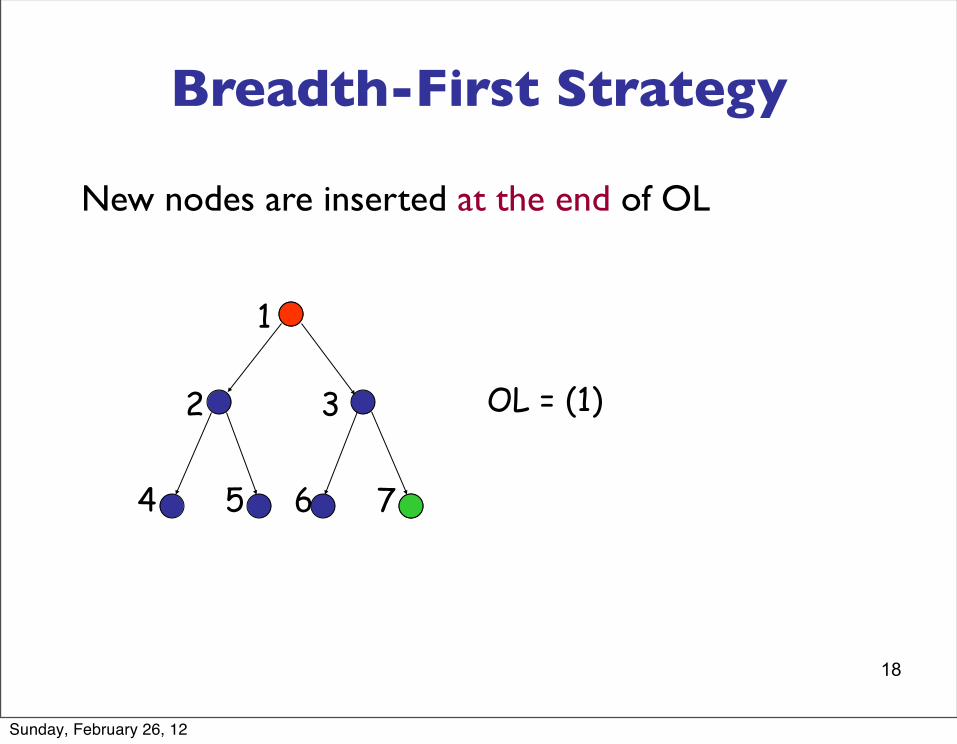
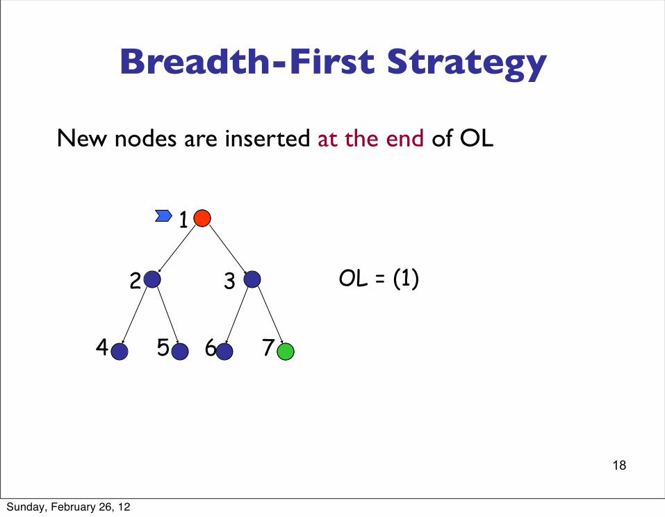
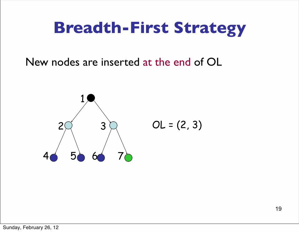
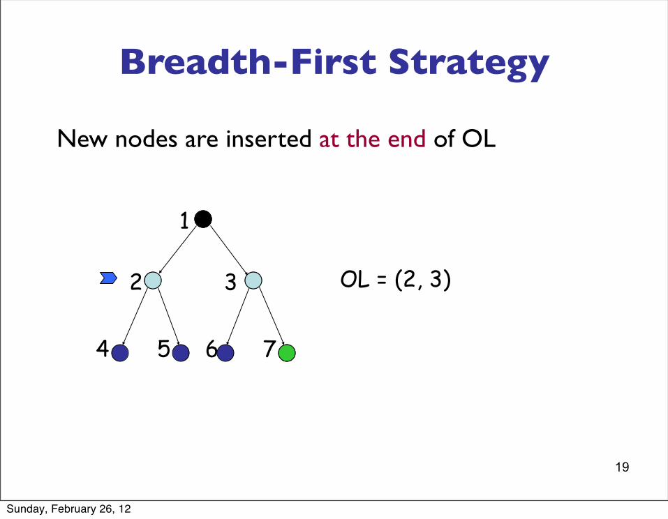
Breadth-First Strategy
New nodes are inserted at the end of OL
2 3
4 5
1
6 7
Sunday, February 26, 12
18
Breadth-First Strategy
New nodes are inserted at the end of OL
2 3
4 5
1
6 7
OL = (1)
Sunday, February 26, 12
18
Breadth-First Strategy
New nodes are inserted at the end of OL
2 3
4 5
1
6 7
OL = (1)
Sunday, February 26, 12
19
Breadth-First Strategy
New nodes are inserted at the end of OL
OL = (2, 3)2 3
4 5
1
6 7
Sunday, February 26, 12
19
Breadth-First Strategy
New nodes are inserted at the end of OL
OL = (2, 3)2 3
4 5
1
6 7
Sunday, February 26, 12
20
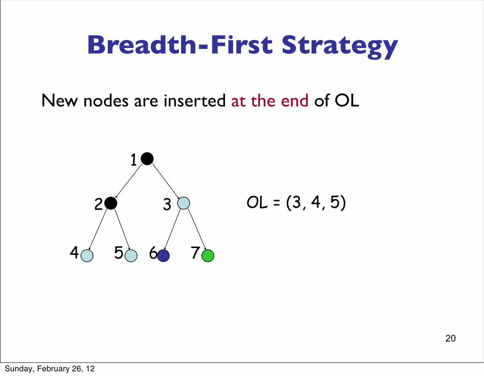
Breadth-First Strategy
New nodes are inserted at the end of OL
OL = (3, 4, 5)2 3
4 5
1
6 7
Sunday, February 26, 12

20
Breadth-First Strategy
New nodes are inserted at the end of OL
OL = (3, 4, 5)2 3
4 5
1
6 7
Sunday, February 26, 12
21
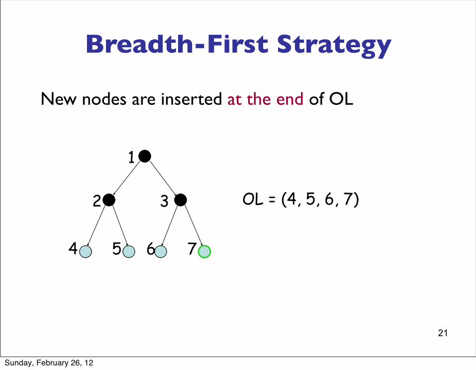
Breadth-First Strategy
New nodes are inserted at the end of OL
OL = (4, 5, 6, 7)2 3
4 5
1
6 7
Sunday, February 26, 12
22
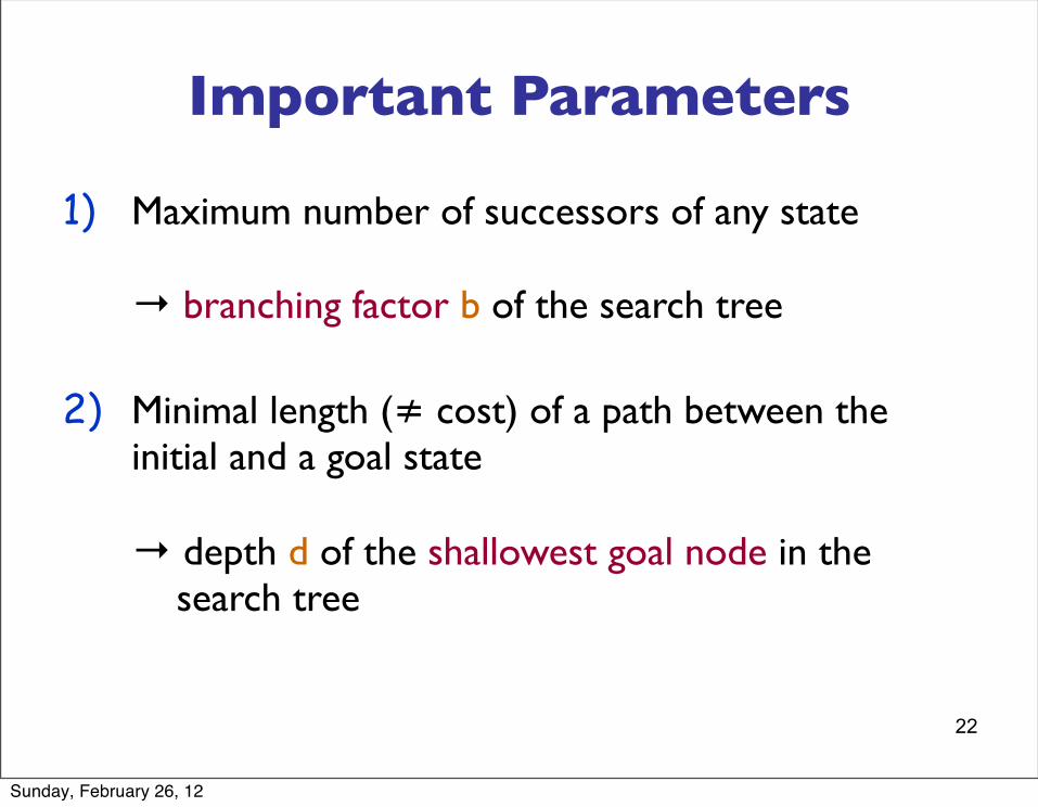
Important Parameters
1) Maximum number of successors of any state
→ branching factor b of the search tree
2) Minimal length (≠ cost) of a path between the initial and a goal state
→ depth d of the shallowest goal node in the search tree
Sunday, February 26, 12
23
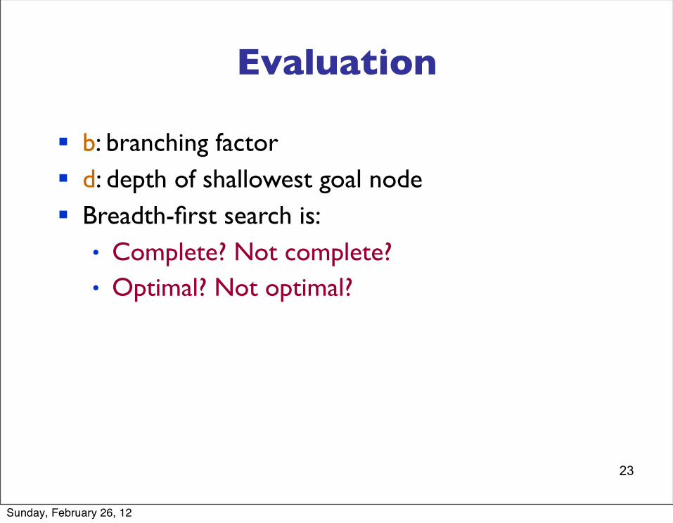
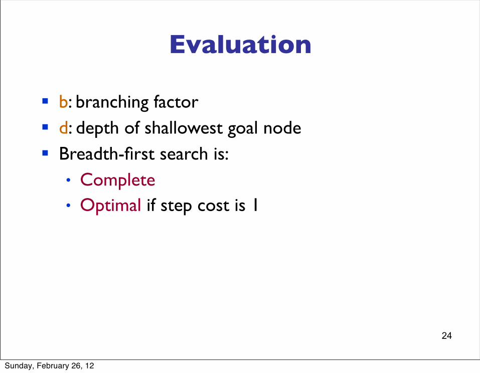
Evaluation
§ b: branching factor§ d: depth of shallowest goal node§ Breadth-first search is:
• Complete? Not complete?• Optimal? Not optimal?
Sunday, February 26, 12

24
Evaluation
Sunday, February 26, 12
24
Evaluation
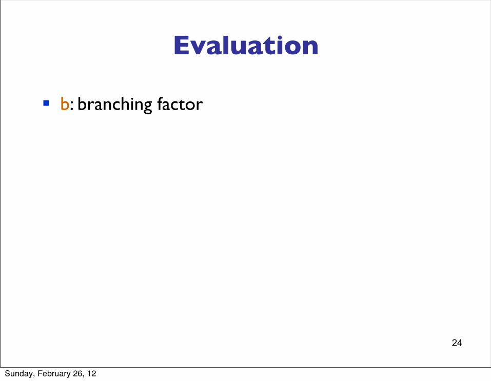
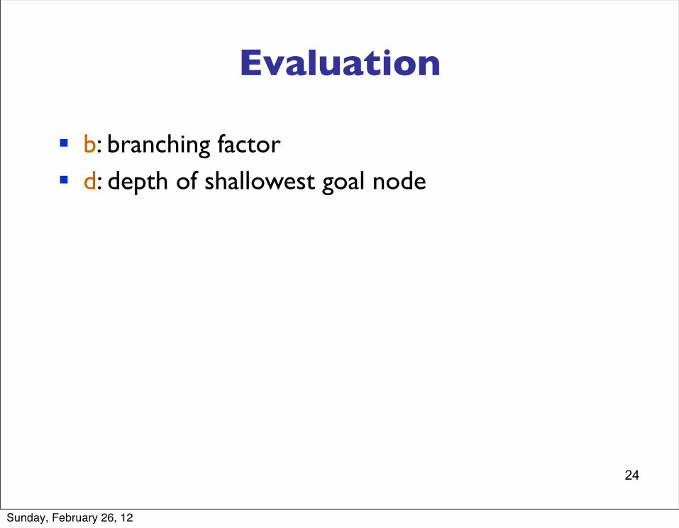
§ b: branching factor
Sunday, February 26, 12
24
Evaluation
§ b: branching factor§ d: depth of shallowest goal node
Sunday, February 26, 12
24
Evaluation
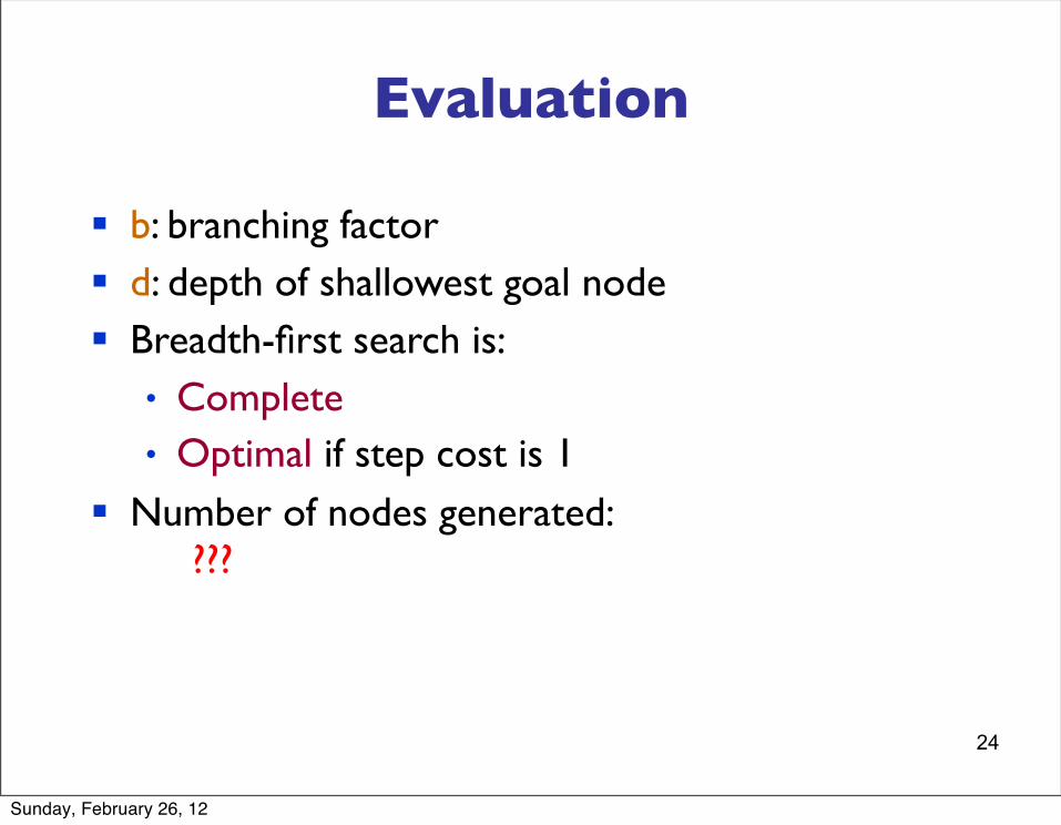
§ b: branching factor§ d: depth of shallowest goal node§ Breadth-first search is:
• Complete• Optimal if step cost is 1
Sunday, February 26, 12
24
Evaluation
§ b: branching factor§ d: depth of shallowest goal node§ Breadth-first search is:
• Complete• Optimal if step cost is 1
§ Number of nodes generated: ???
Sunday, February 26, 12
25
Evaluation
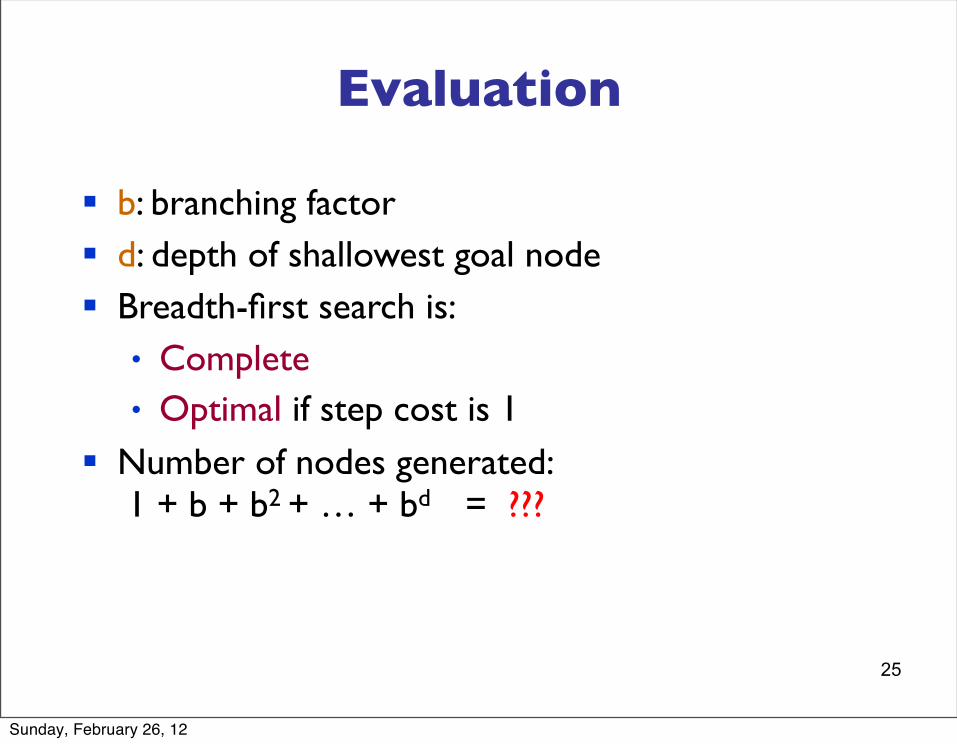
§ b: branching factor§ d: depth of shallowest goal node§ Breadth-first search is:
• Complete• Optimal if step cost is 1
§ Number of nodes generated: 1 + b + b2 + … + bd = ???
Sunday, February 26, 12
26
Evaluation
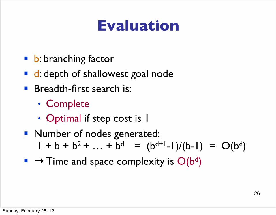
§ b: branching factor§ d: depth of shallowest goal node§ Breadth-first search is:
• Complete• Optimal if step cost is 1
§ Number of nodes generated: 1 + b + b2 + … + bd = (bd+1-1)/(b-1) = O(bd)
§ → Time and space complexity is O(bd)
Sunday, February 26, 12
27
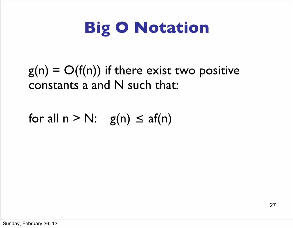
Big O Notation
g(n) = O(f(n)) if there exist two positive constants a and N such that:
for all n > N: g(n) ≤ af(n)
Sunday, February 26, 12
28
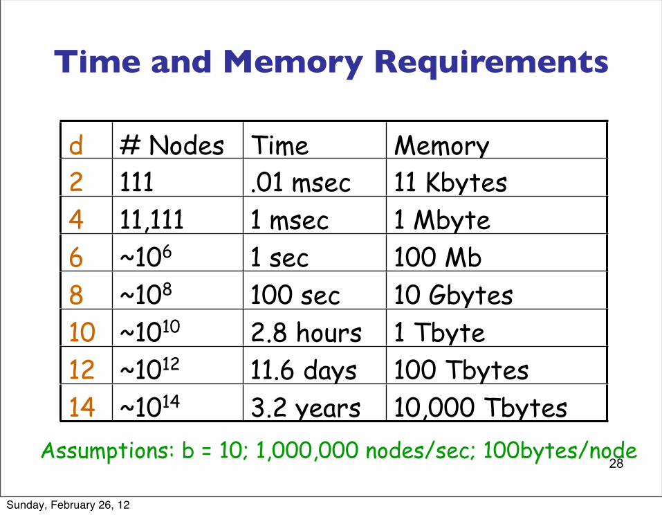
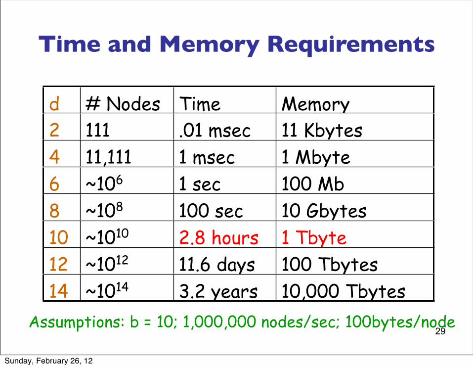
Time and Memory Requirements
d # Nodes Time Memory2 111 .01 msec 11 Kbytes4 11,111 1 msec 1 Mbyte6 ~106 1 sec 100 Mb8 ~108 100 sec 10 Gbytes10 ~1010 2.8 hours 1 Tbyte12 ~1012 11.6 days 100 Tbytes14 ~1014 3.2 years 10,000 Tbytes
Assumptions: b = 10; 1,000,000 nodes/sec; 100bytes/node
Sunday, February 26, 12
29
Time and Memory Requirements
d # Nodes Time Memory2 111 .01 msec 11 Kbytes4 11,111 1 msec 1 Mbyte6 ~106 1 sec 100 Mb8 ~108 100 sec 10 Gbytes10 ~1010 2.8 hours 1 Tbyte12 ~1012 11.6 days 100 Tbytes14 ~1014 3.2 years 10,000 Tbytes
Assumptions: b = 10; 1,000,000 nodes/sec; 100bytes/node
Sunday, February 26, 12
30
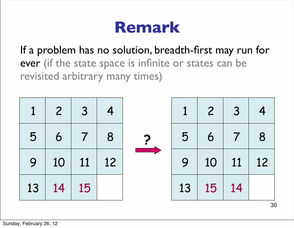
RemarkIf a problem has no solution, breadth-first may run for ever (if the state space is infinite or states can be revisited arbitrary many times)
12
14
11
15
10
13
9
5 6 7 8
4321
12
15
11
14
10
13
9
5 6 7 8
4321
?
Sunday, February 26, 12
31
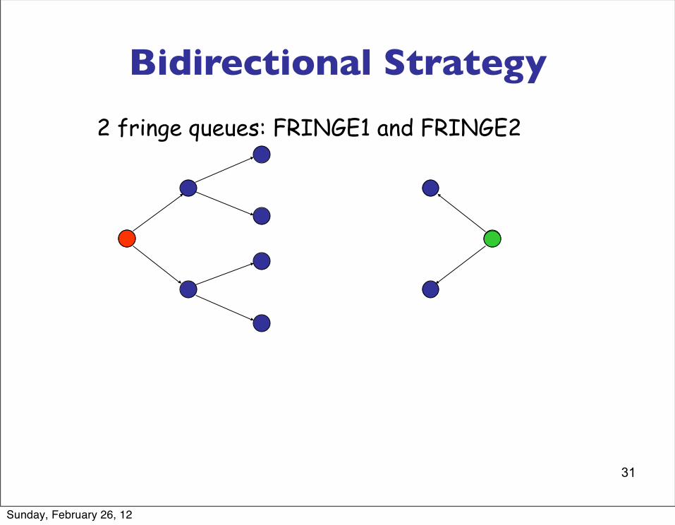
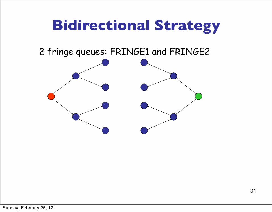
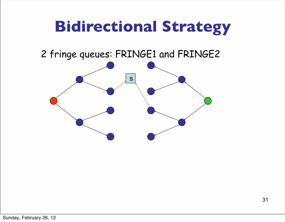
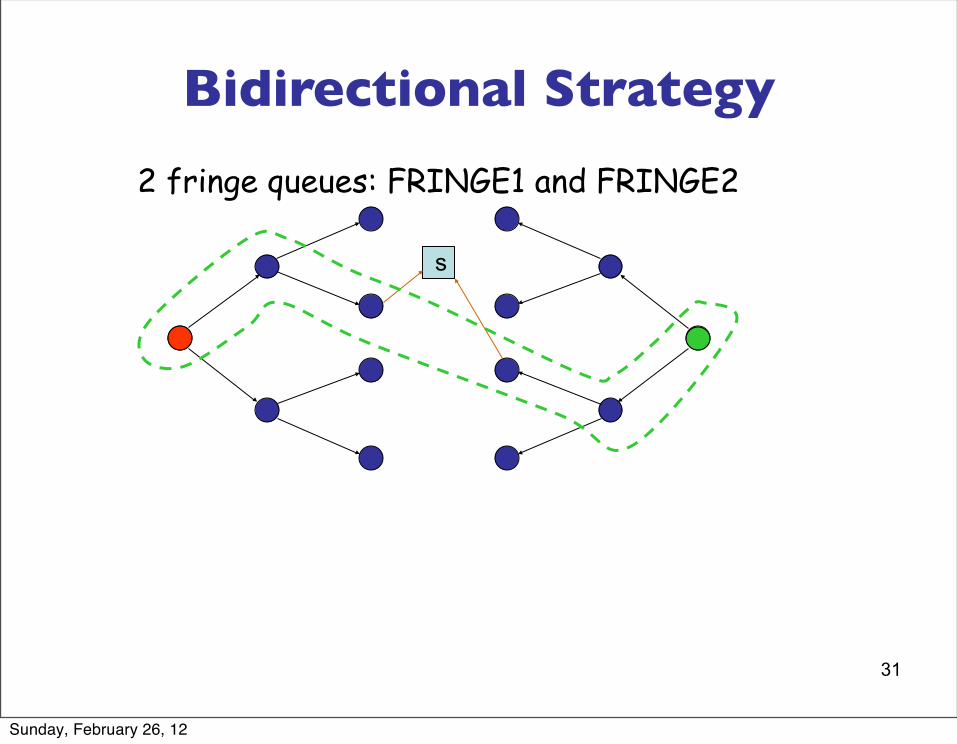
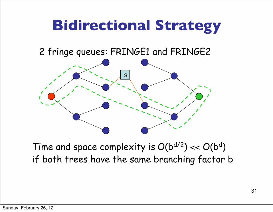
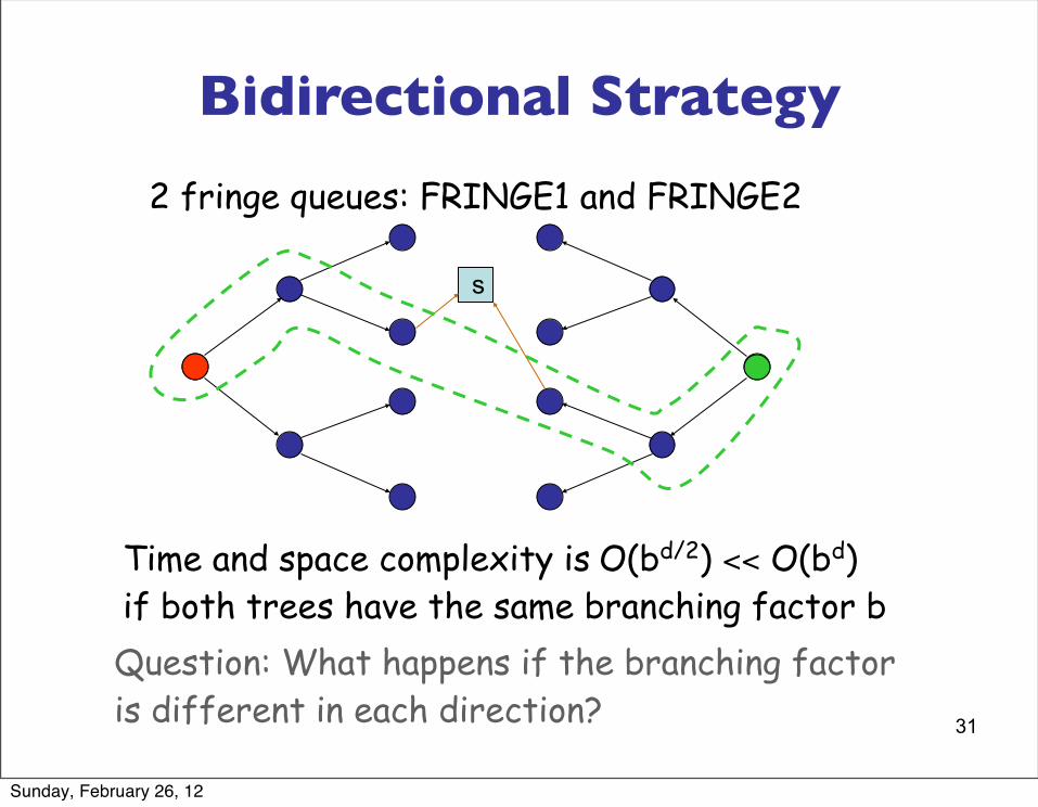
Bidirectional Strategy
Sunday, February 26, 12
31
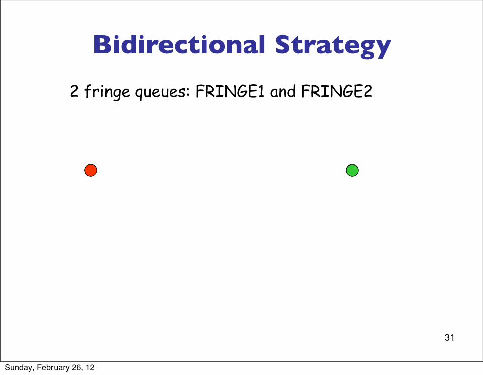
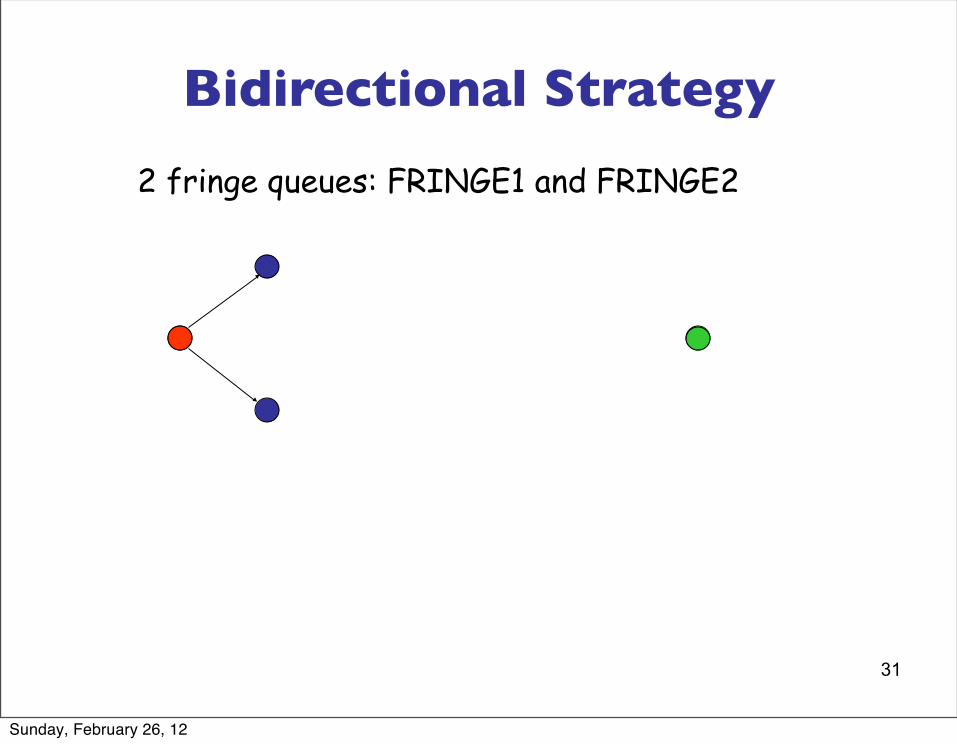
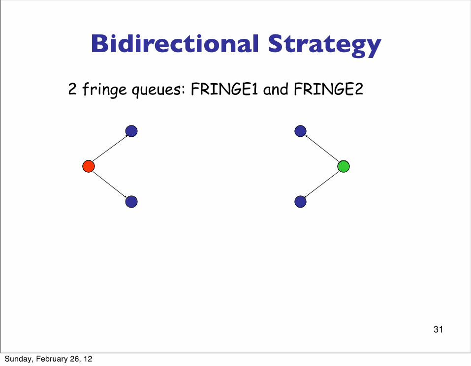
Bidirectional Strategy
2 fringe queues: FRINGE1 and FRINGE2
Sunday, February 26, 12
31
Bidirectional Strategy
2 fringe queues: FRINGE1 and FRINGE2
Sunday, February 26, 12
31
Bidirectional Strategy
2 fringe queues: FRINGE1 and FRINGE2
Sunday, February 26, 12
31
Bidirectional Strategy
2 fringe queues: FRINGE1 and FRINGE2
Sunday, February 26, 12
31
Bidirectional Strategy
2 fringe queues: FRINGE1 and FRINGE2
Sunday, February 26, 12
31
Bidirectional Strategy
2 fringe queues: FRINGE1 and FRINGE2
s
Sunday, February 26, 12
31
Bidirectional Strategy
2 fringe queues: FRINGE1 and FRINGE2
s
Sunday, February 26, 12
31
Bidirectional Strategy
2 fringe queues: FRINGE1 and FRINGE2
s
Time and space complexity is O(bd/2) << O(bd) if both trees have the same branching factor b
Sunday, February 26, 12
31
Bidirectional Strategy
2 fringe queues: FRINGE1 and FRINGE2
s
Time and space complexity is O(bd/2) << O(bd) if both trees have the same branching factor bQuestion: What happens if the branching factor is different in each direction?
Sunday, February 26, 12
32
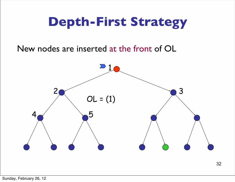
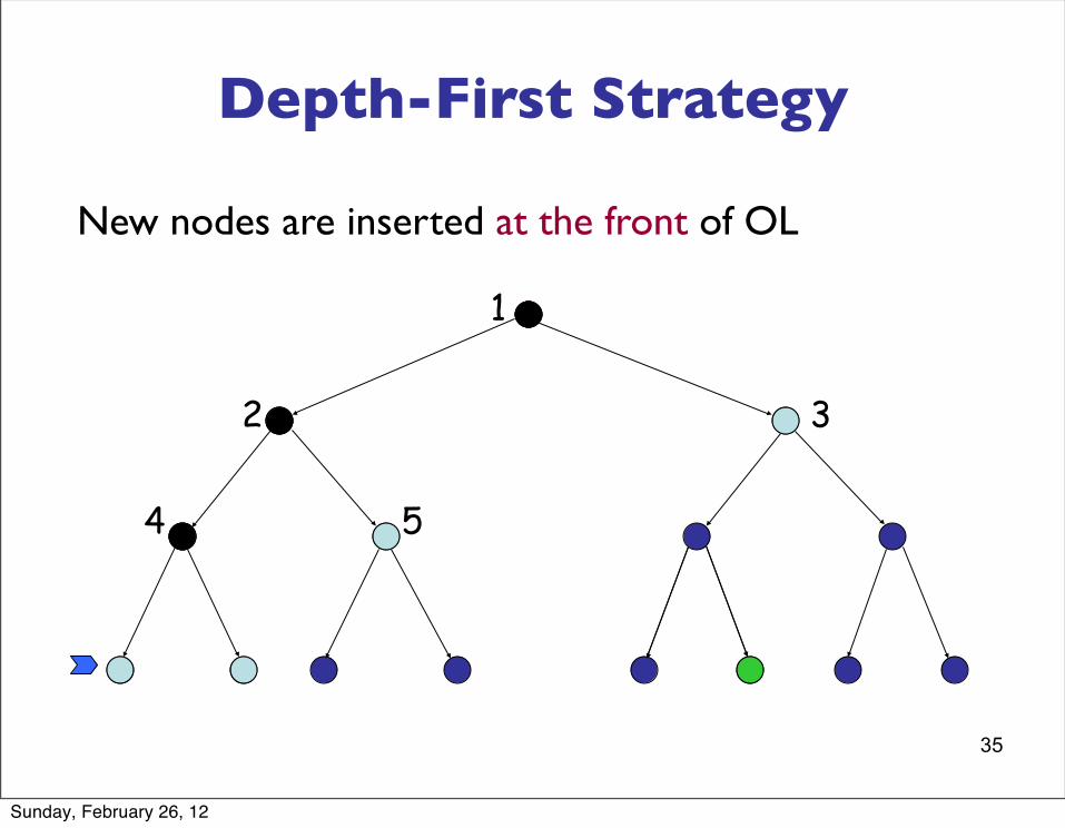
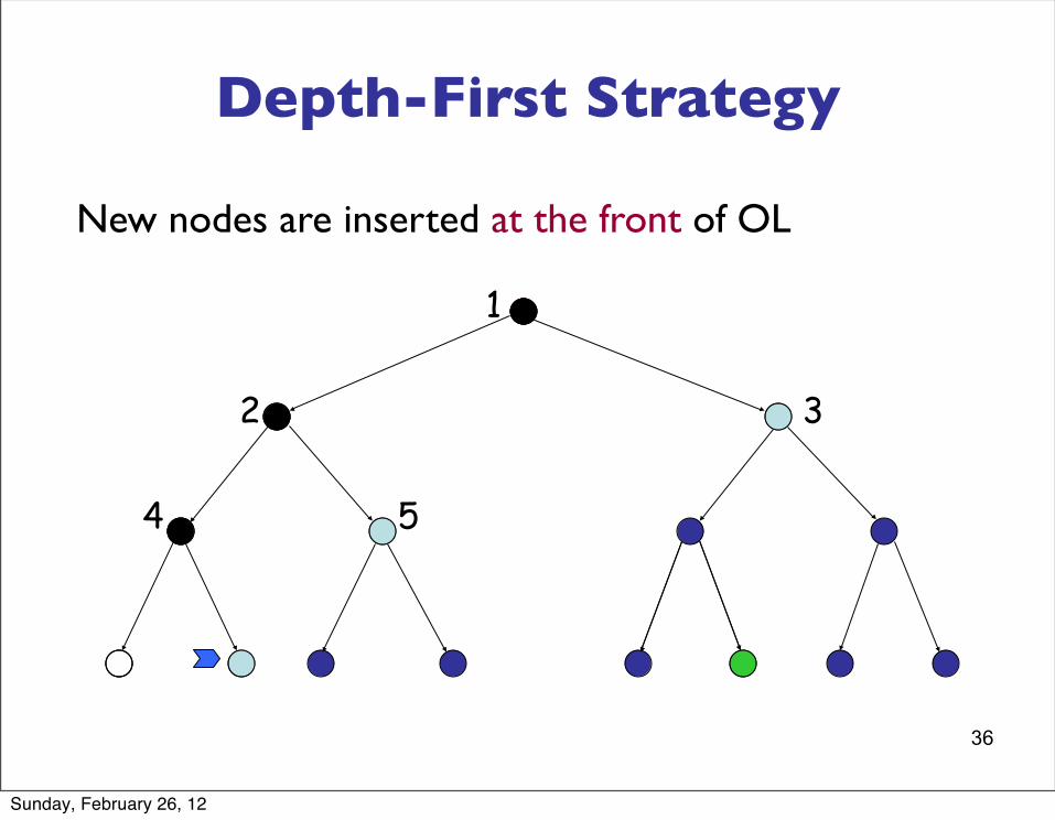
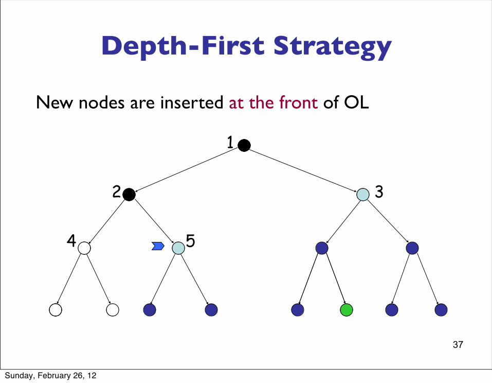
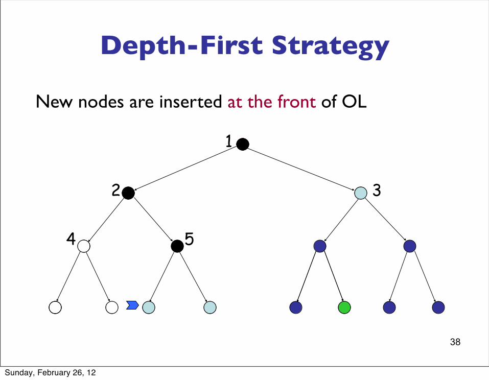
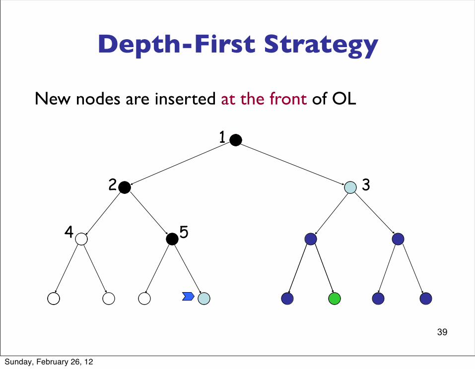
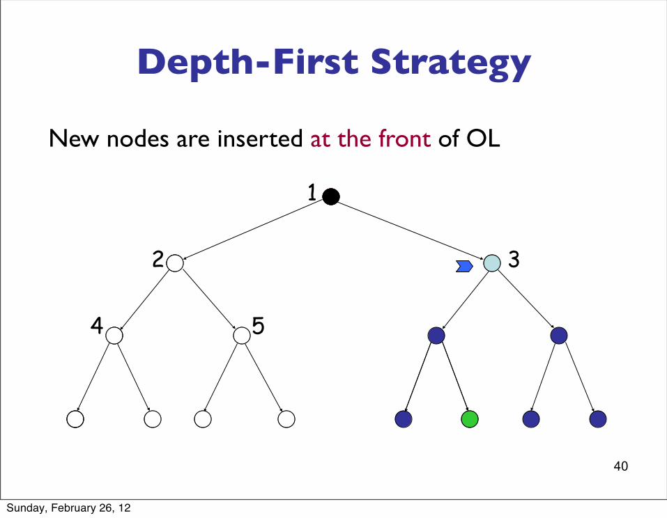
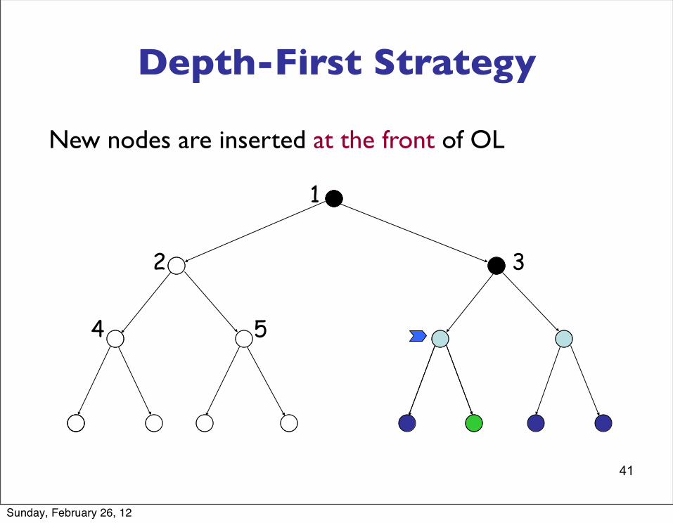
Depth-First Strategy
New nodes are inserted at the front of OL
1
2 3
4 5
OL = (1)
Sunday, February 26, 12
33
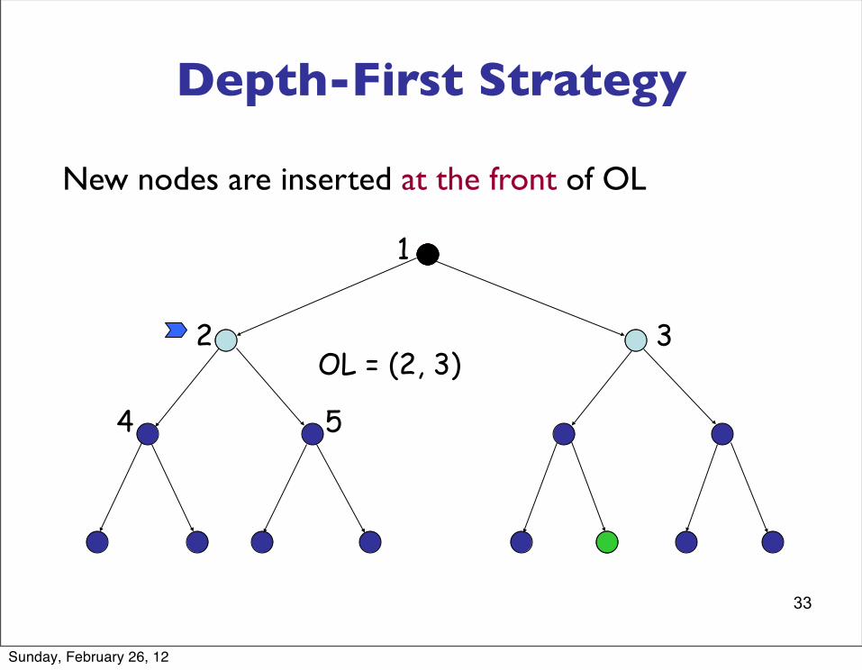
Depth-First Strategy
New nodes are inserted at the front of OL
1
2 3
4 5
OL = (2, 3)
Sunday, February 26, 12

34
Depth-First Strategy
New nodes are inserted at the front of OL
1
2 3
4 5
OL = (4, 5, 3)
Sunday, February 26, 12
35
Depth-First Strategy
New nodes are inserted at the front of OL
1
2 3
4 5
Sunday, February 26, 12
36
Depth-First Strategy
New nodes are inserted at the front of OL
1
2 3
4 5
Sunday, February 26, 12
37
Depth-First Strategy
New nodes are inserted at the front of OL
1
2 3
4 5
Sunday, February 26, 12
38
Depth-First Strategy
New nodes are inserted at the front of OL
1
2 3
4 5
Sunday, February 26, 12
39
Depth-First Strategy
New nodes are inserted at the front of OL
1
2 3
4 5
Sunday, February 26, 12
40
Depth-First Strategy
New nodes are inserted at the front of OL
1
2 3
4 5
Sunday, February 26, 12
41
Depth-First Strategy
New nodes are inserted at the front of OL
1
2 3
4 5
Sunday, February 26, 12

42
Depth-First Strategy
New nodes are inserted at the front of OL
1
2 3
4 5
Sunday, February 26, 12
43
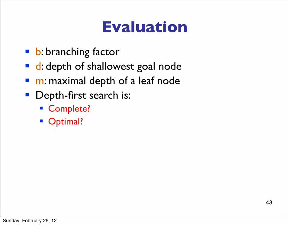
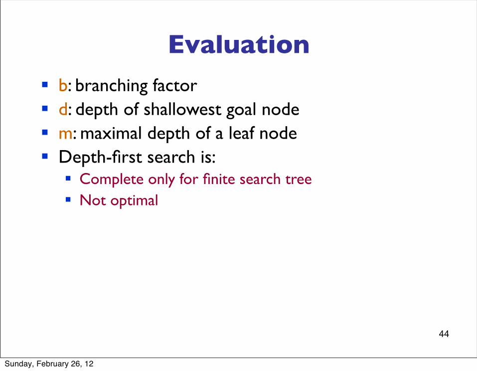
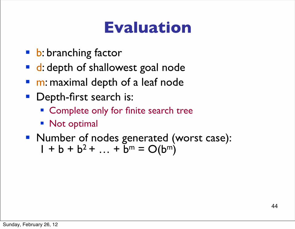
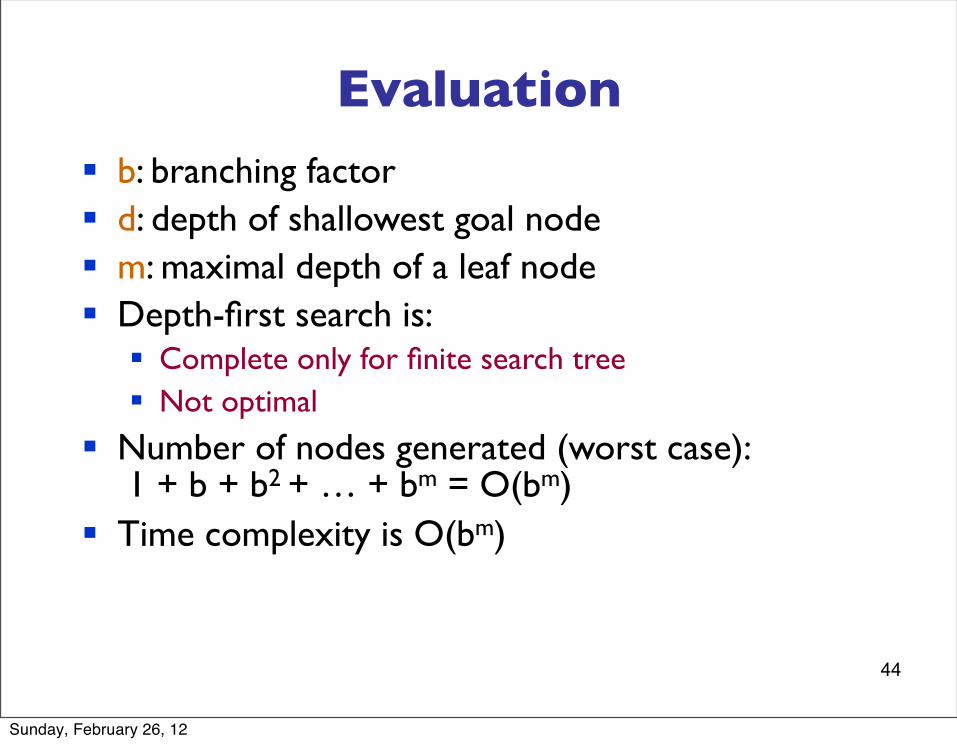
Evaluation§ b: branching factor§ d: depth of shallowest goal node § m: maximal depth of a leaf node§ Depth-first search is:
§ Complete?§ Optimal?
Sunday, February 26, 12

44
Evaluation
Sunday, February 26, 12
44
Evaluation§ b: branching factor§ d: depth of shallowest goal node
Sunday, February 26, 12
44
Evaluation§ b: branching factor§ d: depth of shallowest goal node § m: maximal depth of a leaf node§ Depth-first search is:
§ Complete only for finite search tree§ Not optimal
Sunday, February 26, 12
44
Evaluation§ b: branching factor§ d: depth of shallowest goal node § m: maximal depth of a leaf node§ Depth-first search is:
§ Complete only for finite search tree§ Not optimal
§ Number of nodes generated (worst case): 1 + b + b2 + … + bm = O(bm)
Sunday, February 26, 12
44
Evaluation§ b: branching factor§ d: depth of shallowest goal node § m: maximal depth of a leaf node§ Depth-first search is:
§ Complete only for finite search tree§ Not optimal
§ Number of nodes generated (worst case): 1 + b + b2 + … + bm = O(bm)
§ Time complexity is O(bm)
Sunday, February 26, 12
45
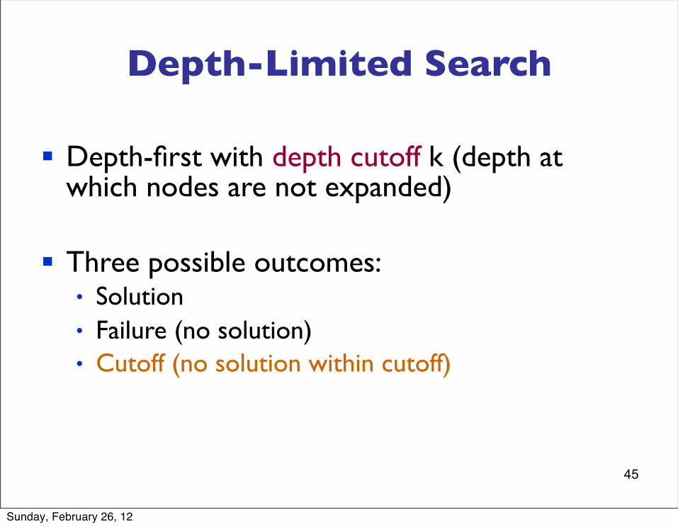
Depth-Limited Search
§ Depth-first with depth cutoff k (depth at which nodes are not expanded)
§ Three possible outcomes:• Solution• Failure (no solution)• Cutoff (no solution within cutoff)
Sunday, February 26, 12
46
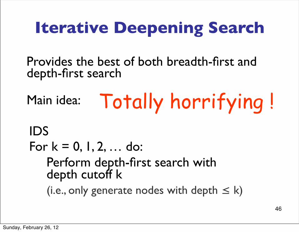
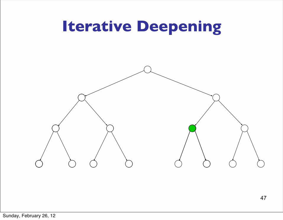
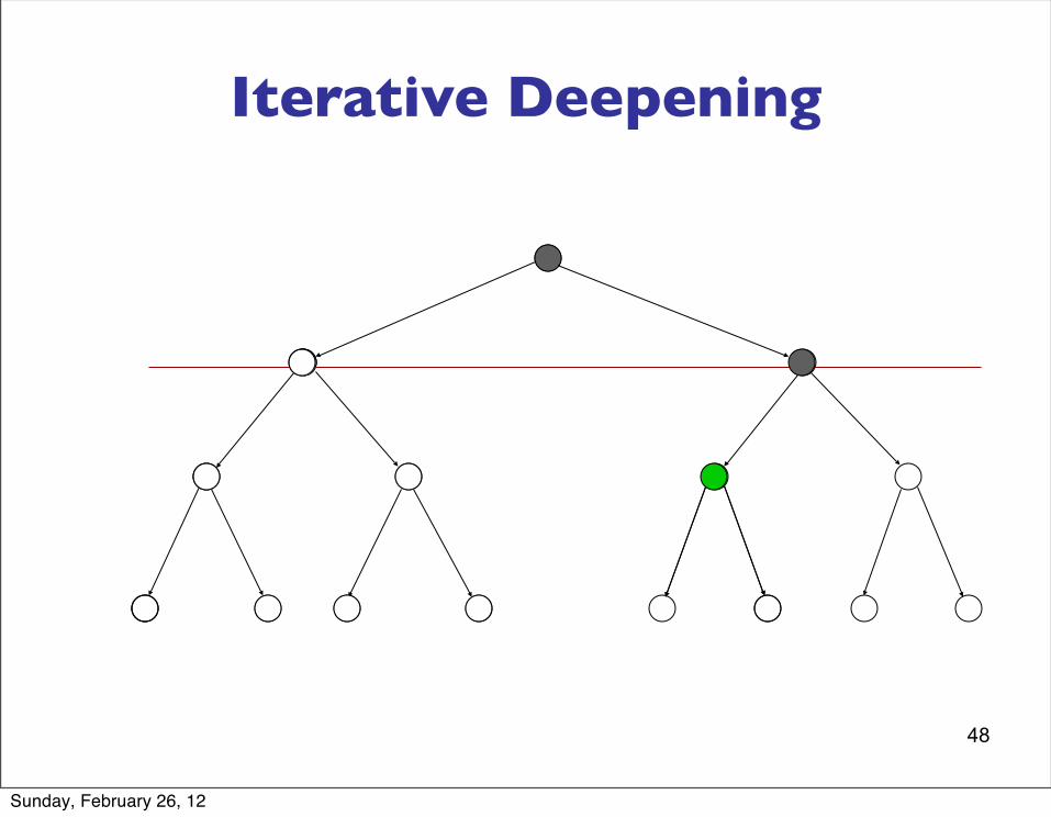
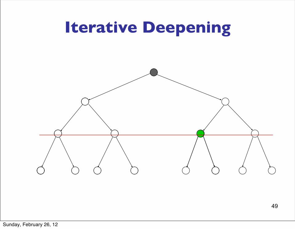
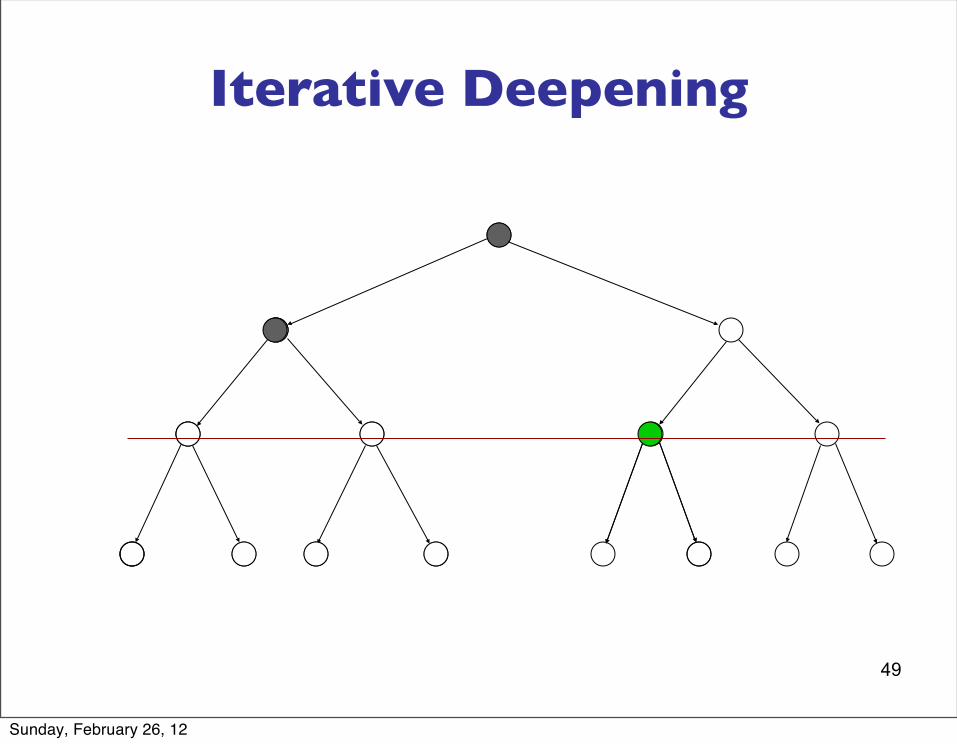
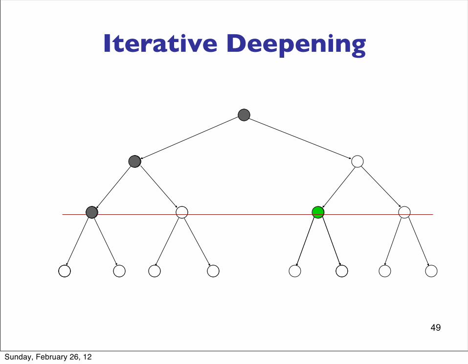
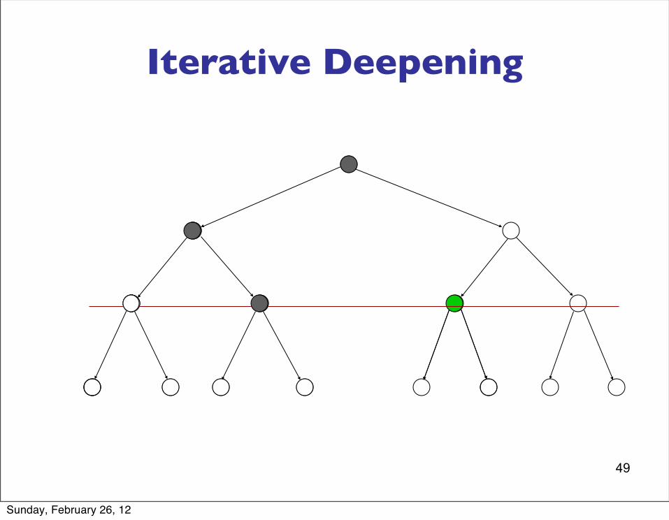
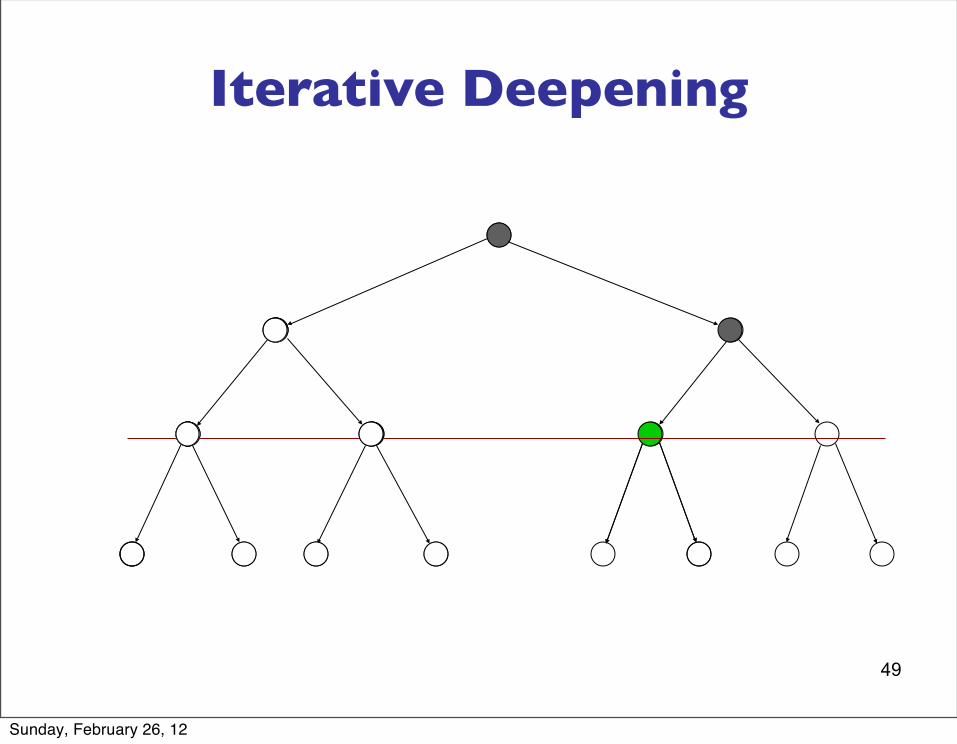
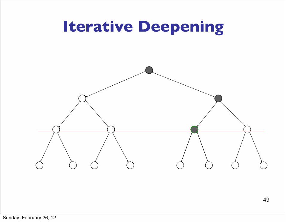
Iterative Deepening Search
Provides the best of both breadth-first and depth-first search
Main idea: Totally horrifying !
Sunday, February 26, 12
46
Iterative Deepening Search
Provides the best of both breadth-first and depth-first search
Main idea: Totally horrifying !
Sunday, February 26, 12
46
Iterative Deepening Search
Provides the best of both breadth-first and depth-first search
Main idea:
IDS For k = 0, 1, 2, … do: Perform depth-first search with depth cutoff k (i.e., only generate nodes with depth ≤ k)
Totally horrifying !
Sunday, February 26, 12
47
Iterative Deepening
Sunday, February 26, 12

47
Iterative Deepening
Sunday, February 26, 12

47
Iterative Deepening
Sunday, February 26, 12

48
Iterative Deepening
Sunday, February 26, 12

48
Iterative Deepening
Sunday, February 26, 12

48
Iterative Deepening
Sunday, February 26, 12
48
Iterative Deepening
Sunday, February 26, 12

49
Iterative Deepening
Sunday, February 26, 12
49
Iterative Deepening
Sunday, February 26, 12
49
Iterative Deepening
Sunday, February 26, 12
49
Iterative Deepening
Sunday, February 26, 12
49
Iterative Deepening
Sunday, February 26, 12
49
Iterative Deepening
Sunday, February 26, 12
49
Iterative Deepening
Sunday, February 26, 12
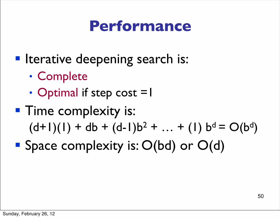
50
Performance
§ Iterative deepening search is:• Complete• Optimal if step cost =1
§ Time complexity is: (d+1)(1) + db + (d-1)b2 + … + (1) bd = O(bd)
§ Space complexity is: O(bd) or O(d)
Sunday, February 26, 12
51
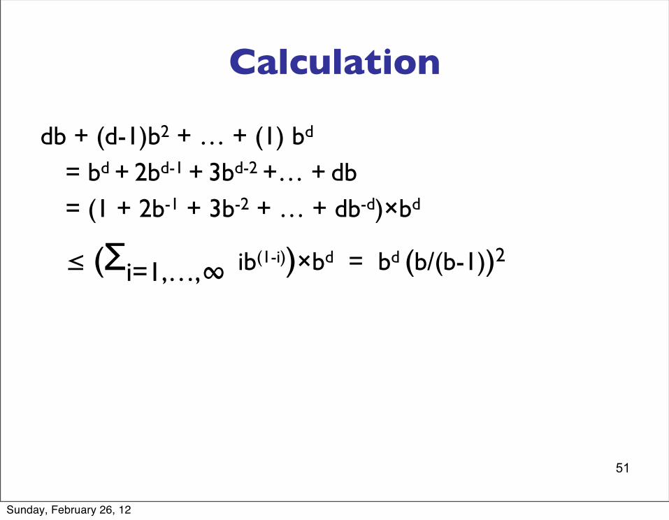
Calculation
db + (d-1)b2 + … + (1) bd
= bd + 2bd-1 + 3bd-2 +… + db = (1 + 2b-1 + 3b-2 + … + db-d)×bd
≤ (Σi=1,…,∞ ib(1-i))×bd = bd (b/(b-1))2
Sunday, February 26, 12
52
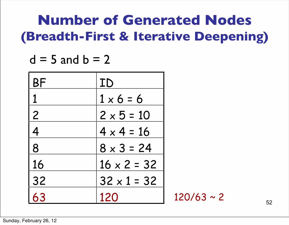
d = 5 and b = 2
BF ID1 1 x 6 = 62 2 x 5 = 104 4 x 4 = 168 8 x 3 = 2416 16 x 2 = 3232 32 x 1 = 3263 120 120/63 ~ 2
Number of Generated Nodes (Breadth-First & Iterative Deepening)
Sunday, February 26, 12
53
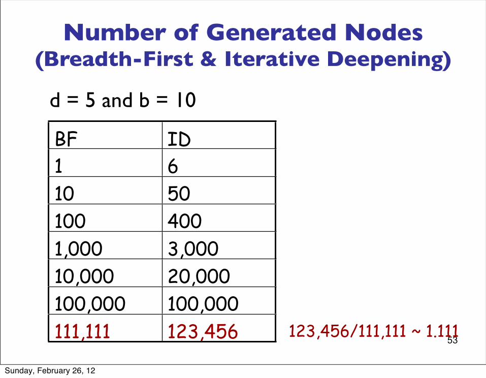
Number of Generated Nodes (Breadth-First & Iterative Deepening)
d = 5 and b = 10
BF ID1 610 50100 4001,000 3,00010,000 20,000100,000 100,000111,111 123,456 123,456/111,111 ~ 1.111
Sunday, February 26, 12
54
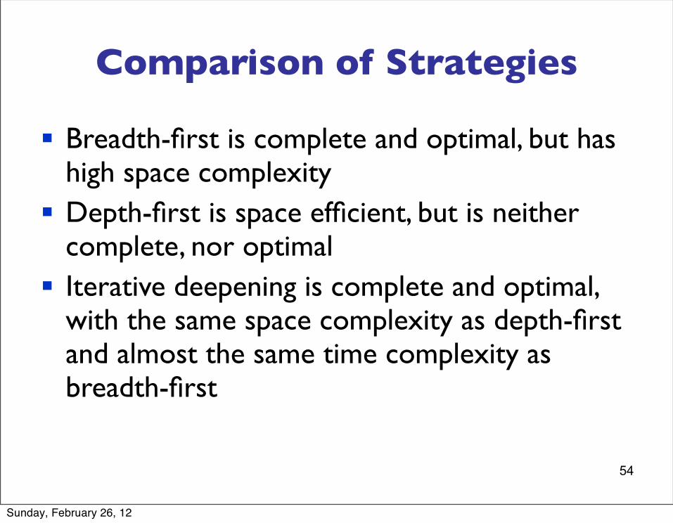
Comparison of Strategies
§ Breadth-first is complete and optimal, but has high space complexity
§ Depth-first is space efficient, but is neither complete, nor optimal
§ Iterative deepening is complete and optimal, with the same space complexity as depth-first and almost the same time complexity as breadth-first
Sunday, February 26, 12
55
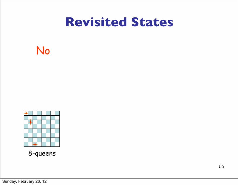
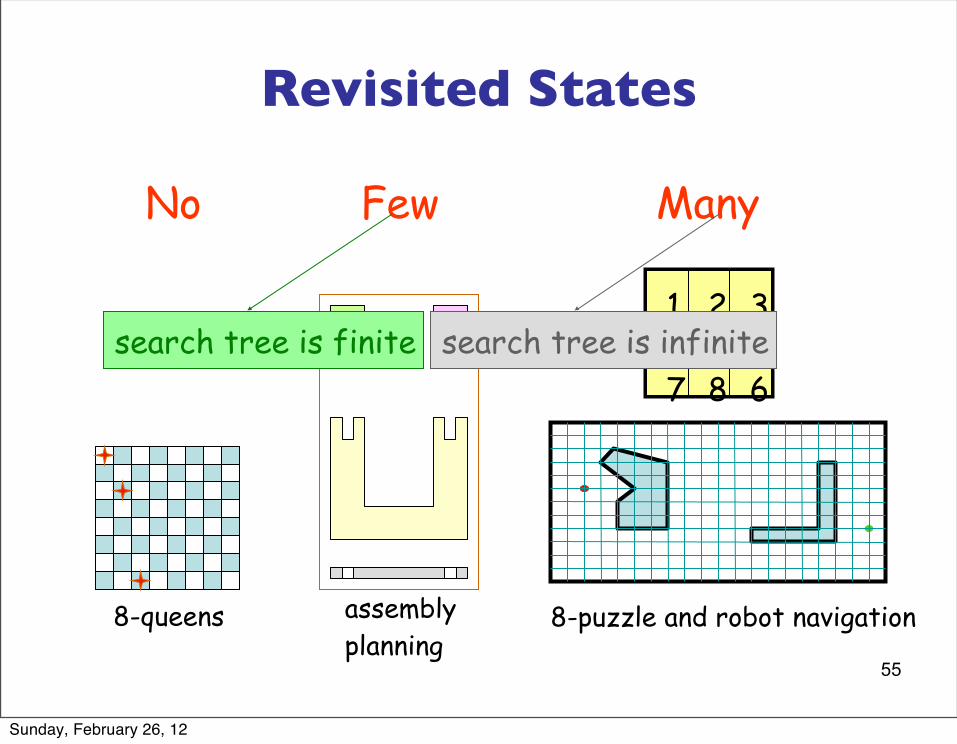
Revisited States
Sunday, February 26, 12
55
Revisited States
8-queens
No
Sunday, February 26, 12
55
Revisited States
8-queens
No
assembly planning
Few
Sunday, February 26, 12

55
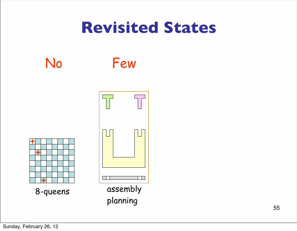
Revisited States
8-queens
No
assembly planning
Few
search tree is finite
Sunday, February 26, 12

55
Revisited States
8-queens
No
assembly planning
Few
1 2 34 5
67 8
8-puzzle and robot navigation
Many
search tree is finite
Sunday, February 26, 12
55
Revisited States
8-queens
No
assembly planning
Few
1 2 34 5
67 8
8-puzzle and robot navigation
Many
search tree is finite search tree is infinite
Sunday, February 26, 12
56
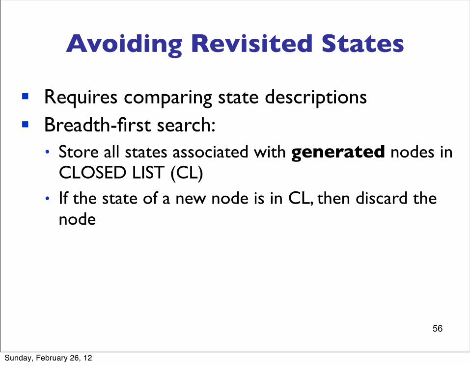
Avoiding Revisited States
§ Requires comparing state descriptions § Breadth-first search:
• Store all states associated with generated nodes in CLOSED LIST (CL)
• If the state of a new node is in CL, then discard the node
Sunday, February 26, 12

59
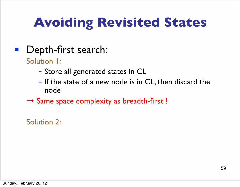
Avoiding Revisited States
Sunday, February 26, 12
59
Avoiding Revisited States
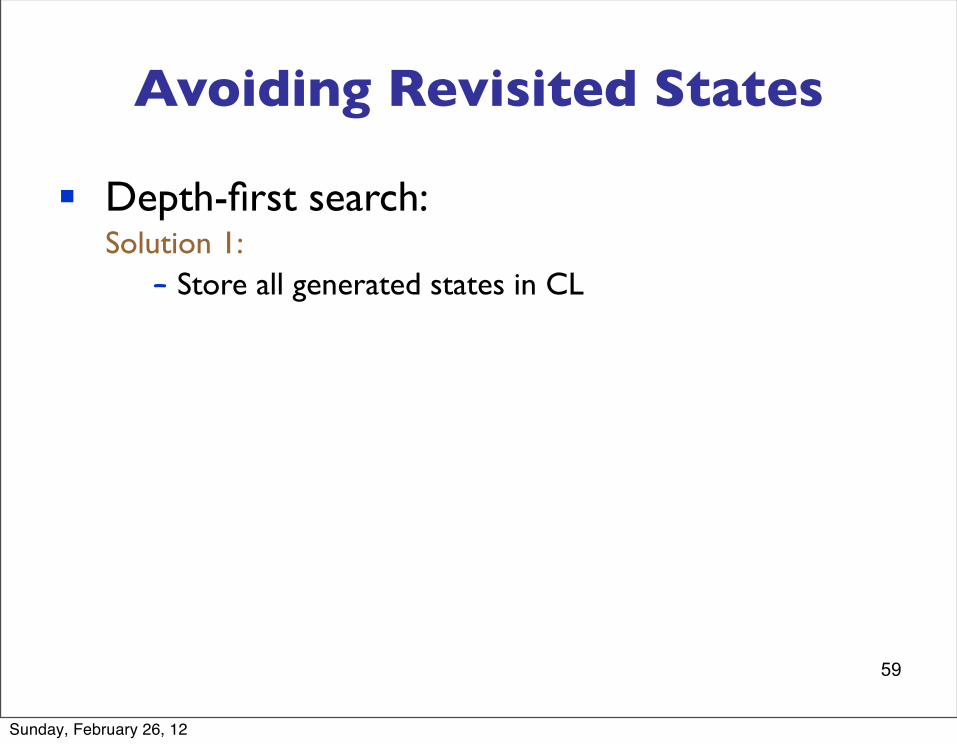
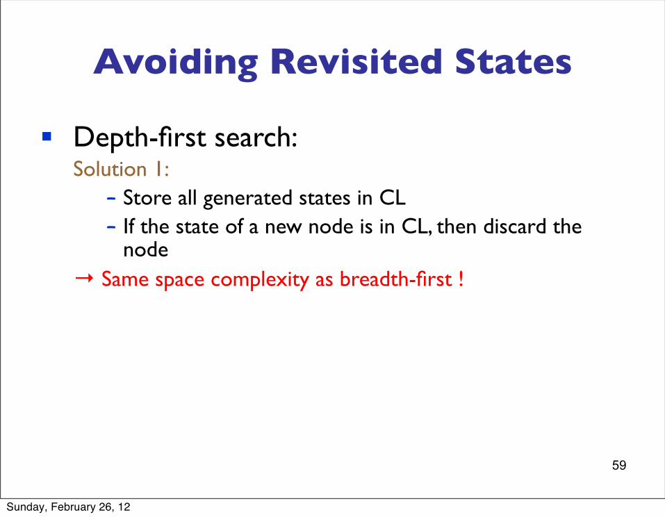
§ Depth-first search: Solution 1:
– Store all generated states in CL
Sunday, February 26, 12

59
Avoiding Revisited States
§ Depth-first search: Solution 1:
– Store all generated states in CL– If the state of a new node is in CL, then discard the
node
Sunday, February 26, 12
59
Avoiding Revisited States
§ Depth-first search: Solution 1:
– Store all generated states in CL– If the state of a new node is in CL, then discard the
node→ Same space complexity as breadth-first !
Sunday, February 26, 12

59
Avoiding Revisited States
Sunday, February 26, 12

59
Avoiding Revisited States
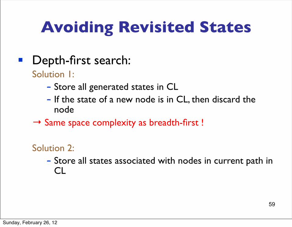
§ Depth-first search: Solution 1:
– Store all generated states in CL
Sunday, February 26, 12

59
Avoiding Revisited States
§ Depth-first search: Solution 1:
– Store all generated states in CL– If the state of a new node is in CL, then discard the
node
Sunday, February 26, 12

59
Avoiding Revisited States
§ Depth-first search: Solution 1:
– Store all generated states in CL– If the state of a new node is in CL, then discard the
node→ Same space complexity as breadth-first !
Sunday, February 26, 12

59
Avoiding Revisited States
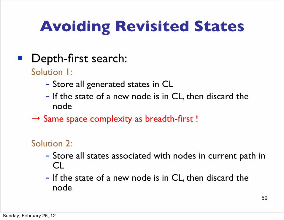
§ Depth-first search: Solution 1:
– Store all generated states in CL– If the state of a new node is in CL, then discard the
node→ Same space complexity as breadth-first !
Sunday, February 26, 12
59
Avoiding Revisited States
§ Depth-first search: Solution 1:
– Store all generated states in CL– If the state of a new node is in CL, then discard the
node→ Same space complexity as breadth-first !
Solution 2:
Sunday, February 26, 12
59
Avoiding Revisited States
§ Depth-first search: Solution 1:
– Store all generated states in CL– If the state of a new node is in CL, then discard the
node→ Same space complexity as breadth-first !
Solution 2:– Store all states associated with nodes in current path in
CL
Sunday, February 26, 12
59
Avoiding Revisited States
§ Depth-first search: Solution 1:
– Store all generated states in CL– If the state of a new node is in CL, then discard the
node→ Same space complexity as breadth-first !
Solution 2:– Store all states associated with nodes in current path in
CL– If the state of a new node is in CL, then discard the
node
Sunday, February 26, 12

59
Avoiding Revisited States
§ Depth-first search: Solution 1:
– Store all generated states in CL– If the state of a new node is in CL, then discard the
node→ Same space complexity as breadth-first !
Solution 2:– Store all states associated with nodes in current path in
CL– If the state of a new node is in CL, then discard the
nodeà Only avoids loops
Sunday, February 26, 12
60
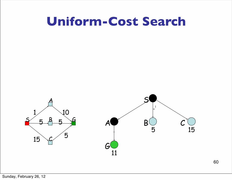
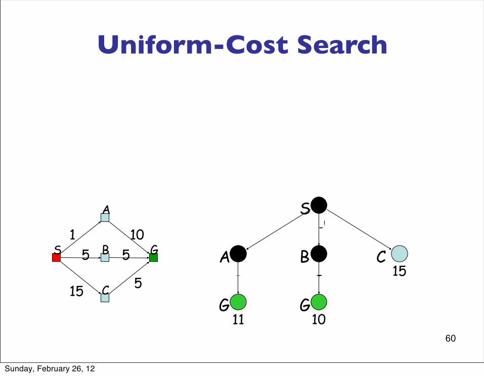
Uniform-Cost Search
Sunday, February 26, 12
60
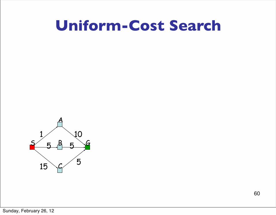
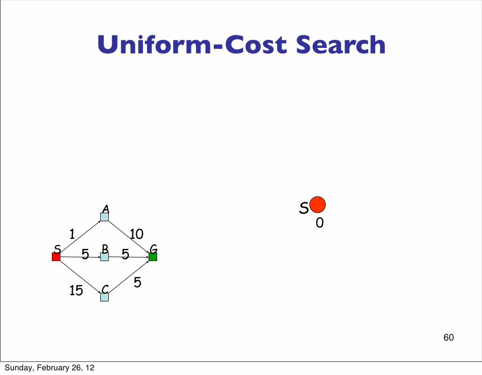
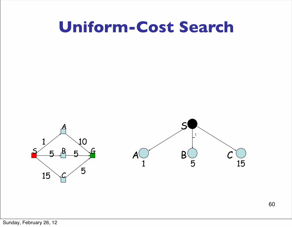
Uniform-Cost Search
S G
A
B
C
51
15
10
5
5
Sunday, February 26, 12
60
Uniform-Cost Search
S0
S G
A
B
C
51
15
10
5
5
Sunday, February 26, 12
60
Uniform-Cost Search
S0
1A
5B
15CS G
A
B
C
51
15
10
5
5
Sunday, February 26, 12
60
Uniform-Cost Search
S0
1A
5B
15CS G
A
B
C
51
15
10
5
5
G11
Sunday, February 26, 12
60
Uniform-Cost Search
S0
1A
5B
15CS G
A
B
C
51
15
10
5
5
G11
G10
Sunday, February 26, 12

60
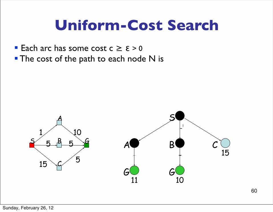
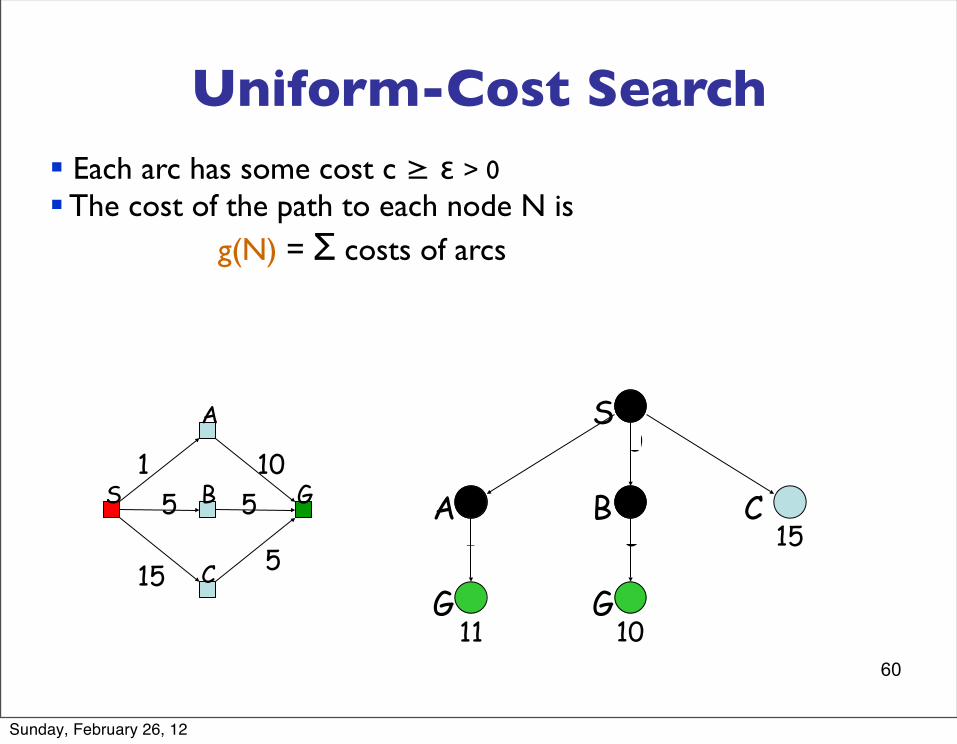
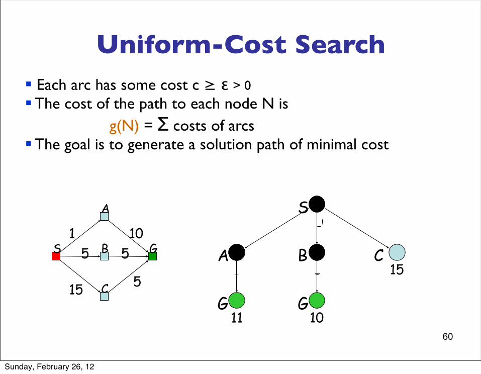
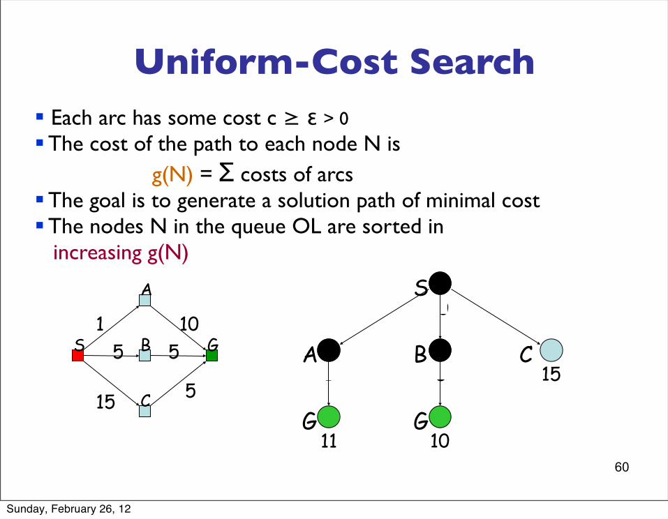
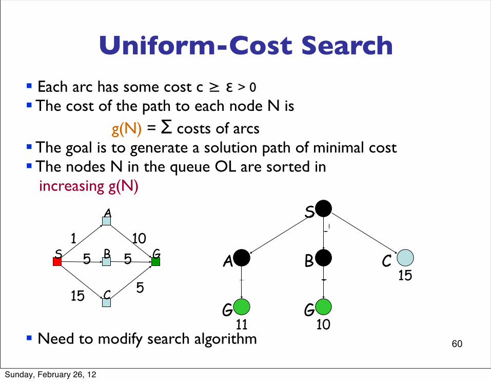
Uniform-Cost Search§ Each arc has some cost c ≥ ε > 0
S0
1A
5B
15CS G
A
B
C
51
15
10
5
5
G11
G10
Sunday, February 26, 12
60
Uniform-Cost Search§ Each arc has some cost c ≥ ε > 0§ The cost of the path to each node N is
S0
1A
5B
15CS G
A
B
C
51
15
10
5
5
G11
G10
Sunday, February 26, 12
60
Uniform-Cost Search§ Each arc has some cost c ≥ ε > 0§ The cost of the path to each node N is g(N) = Σ costs of arcs
S0
1A
5B
15CS G
A
B
C
51
15
10
5
5
G11
G10
Sunday, February 26, 12
60
Uniform-Cost Search§ Each arc has some cost c ≥ ε > 0§ The cost of the path to each node N is g(N) = Σ costs of arcs§ The goal is to generate a solution path of minimal cost
S0
1A
5B
15CS G
A
B
C
51
15
10
5
5
G11
G10
Sunday, February 26, 12
60
Uniform-Cost Search§ Each arc has some cost c ≥ ε > 0§ The cost of the path to each node N is g(N) = Σ costs of arcs§ The goal is to generate a solution path of minimal cost§ The nodes N in the queue OL are sorted in increasing g(N)
§ Need to modify search algorithm
S0
1A
5B
15CS G
A
B
C
51
15
10
5
5
G11
G10
Sunday, February 26, 12
61
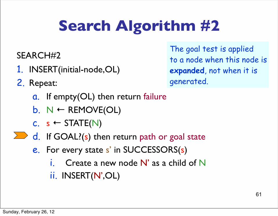
Search Algorithm #2
SEARCH#2
1. INSERT(initial-node,OL)
2. Repeat:
a. If empty(OL) then return failure
b. N ← REMOVE(OL)c. s ← STATE(N)
d. If GOAL?(s) then return path or goal statee. For every state s’ in SUCCESSORS(s)
i. Create a new node N’ as a child of N ii. INSERT(N’,OL)
The goal test is appliedto a node when this node isexpanded, not when it isgenerated.
Sunday, February 26, 12
62
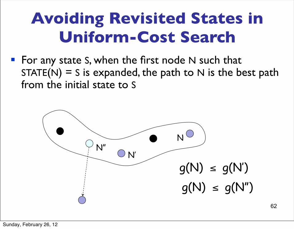
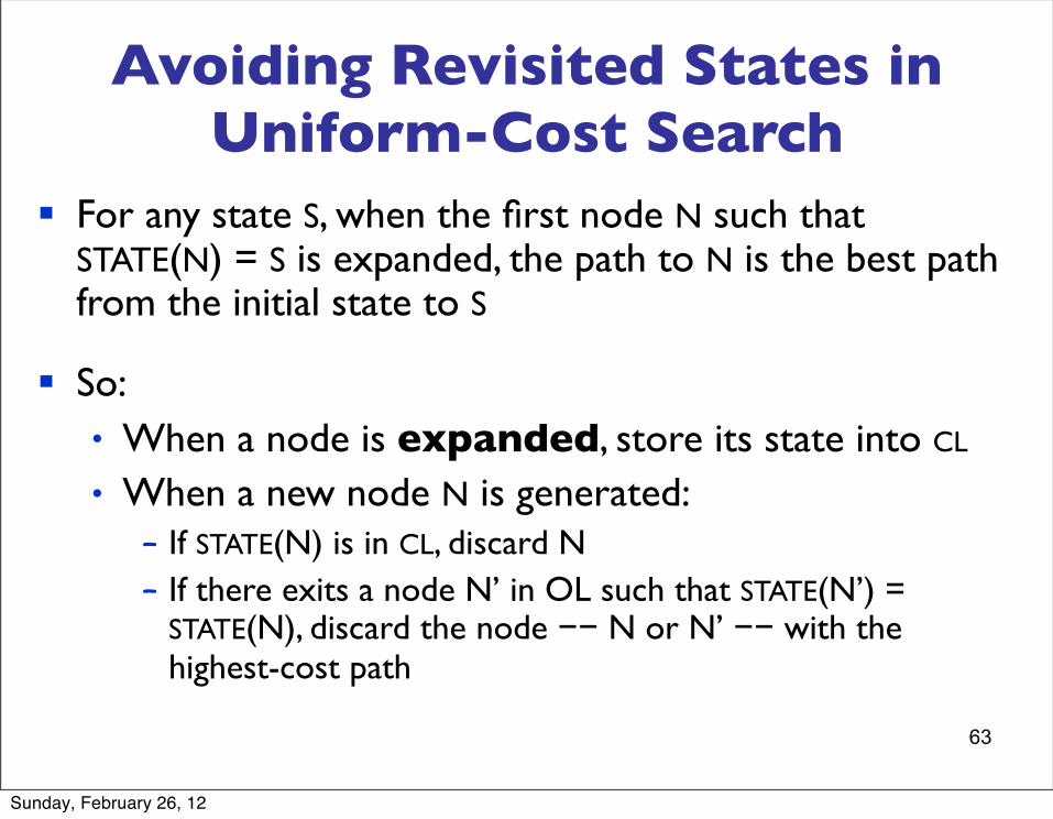
Avoiding Revisited States in Uniform-Cost Search
§ For any state S, when the first node N such that STATE(N) = S is expanded, the path to N is the best path from the initial state to S
N
N’N”
g(N) ≤ g(N’)g(N) ≤ g(N”)
Sunday, February 26, 12
63
Avoiding Revisited States in Uniform-Cost Search
§ For any state S, when the first node N such that STATE(N) = S is expanded, the path to N is the best path from the initial state to S
§ So:• When a node is expanded, store its state into CL • When a new node N is generated:
– If STATE(N) is in CL, discard N– If there exits a node N’ in OL such that STATE(N’) =
STATE(N), discard the node −− N or N’ −− with the highest-cost path
Sunday, February 26, 12