BLIND SOURCE SEPARATION USING FREQUENCY DOMAIN INDEPENDENT COMPONENT

ANALYSIS

Okwelume Gozie Emmanuel Ezeude Anayo Kingsley

This Thesis is presenTed as parT of degree of

MasTer of science in elecTrical engineering

Blekinge Institute of Technology June, 2007

Blekinge Institute of Technology School of Engineering Department of Applied Signal Processing Supervisor: Dr. Nedelko Grbic (Associate Professor) Examiner: Dr. Nedelko Grbic (Associate Professor)

Abstract

The need for speech enhancement is very important, because of the acoustic

environment we are living in, which is composed of noise and other atmospheric

disturbances, and this makes it almost impossible to record a speech signal in pure

form. In most of the mixed signals there is usually no information about each source

such as its location and time distribution. In such situation the estimates of the

original source signals is done based on the information of the received mixed signals,

therefore the approach to be adopted in such cases to separate the signals must be one

that does it blindly, thus the method Blind Source Separation is used in this work.

Our thesis work focuses on Frequency-domain Blind Source Separation (BSS) in

which the received mixed signals are converted into the frequency domain and

Independent Component Analysis (ICA) is applied to instantaneous mixtures at each

frequency bin. Computational complexity is also reduced by using this method.

We also investigate the famous problem associated with Frequency-Domain Blind

Source Separation using ICA referred to as the Permutation and Scaling ambiguities,

using methods proposed by some researchers. This is our main target in this project;

to solve the permutation and scaling ambiguities in real time applications using the

method proposed by Minje et al in [12].

Our results show that this method works far better in an “offline” (i.e. simulated)

mixtures than in real time applications and lastly we gave some suggestions on what

can be done to improve the results.

2

Acknowledgement

With profound humility, we wish to express our gratitude to the Infinite One, the

Almighty God, for all his benevolence, graces and blessing throughout our period of

study in Sweden.

Our special thanks go to our advisor, Associate Prof. Nedelko Grbic for providing us

an opportunity to work with him. He has been such a wonderful adviser, a motivator,

a Teacher and a friend, who is always there with open hands to welcome us and to

assist us in any difficulty despite his tight schedules.

We also wish to express our gratitude to program manager, Mikael Åsman, who is a

good source of encouragement, and to all the staffs and members of the Department

of Telecommunication and signal processing we thank you all.

We want to specially express our sincere appreciation to our parents for their

perseverance, encouragement and most importantly their huge financial support

throughout the journey of academic pursuit and also to our siblings for their words of

encouragement and support.

And lastly to all our friends who supported us throughout the period of this work we

say thank you so much.

3

Table of Content Chapter 1

1.1 Introduction 7

Chapter 2

2.1 Fourier Transform 9

2.2 Short Time Fourier Transform 10

2.2.1 Overlap Save Method 10

2.2.2 Overlap Add Method 13

Chapter 3

3.1 Optimization Methods 17

3.1.1 Vector Gradient 18

3.1.2 Matrix Gradient 20

3.2 Learning Rules for Optimization 20

3.2.1 Gradient Decent 21

3.2.2 Natural Gradient 22

Chapter 4

4.1 Blind Source Separation 25

4.2 Independent Component Analysis 28

4.2.1 Statistical Independent 29

4.2.2 Non-Gaussian Distribution 30

4.3 Measures of Nongaussianity 31

4.3.1 Kurtosis 31

4.3.2 Negentropy 33

4.4 Maximum Likelihood Method 35

4.4.1 Probability Density Function of a Transformed Variable 37

4.4.2 The maximum likelihood of ICA model 37

4

Chapter 5

5.1 Frequency Domain Convolutive BSS/ICA 41

5.1.1 STFT / ISTFT Stage 41

5.1.2 ICA Stage 44

5.1.3 Permutation 47

5.1.4 ICA Based Clustering 48

5.1.5 Scaling 50

5.2 Results 52

Chapter 6

6.1 Conclusion 55

Reference 56

5

List of Figures Fig.2.1: Illustration of Overlap-save method

Fig.2.2: Illustration of Overlap-add method

Fig.3.1: Contour map of assumed cost function.

Fig.4.1: Mixture of two speech sources

Fig.4.2: The schematic diagram of BSS for Convolutive Mixtures

Fig.4.3: Plot of Probability Density Function of some Gaussian distributions.

Fig.4.4: Different well known distribution together with their kurtosis measure

Fig.5.1: Block diagram of Frequency domain BSS/ICA

Fig.5.2: The Power Spectral Density of the sinusoidal signal before STFT

Fig.5.3: The Power Spectral Density of the sinusoidal signal after ISTFT

Fig.5.4: The PSD of ISTFT of the Sinusoidal Signal using Blackman window

Fig.5.5: The plot of the condition of a performance matrix.

Fig.5.6: The plot of hyperbolic tangent of complex number [11]

Fig.5.7: The plot of hyperbolic tangent of parts of complex number [11]

Fig.5.8: The plot of the source and estimated source using ( ) ( )izzzf += tanh as ICA cost

function.

Fig.5.9:The plot of the source and estimated source using

( ) ( ) ( )izzzf ImtanhRetanh += as ICA cost function.

6

Chapter 1

1.1 Introduction

Speech enhancement is very important for applications of speech processing and

communications; in our daily environs we always encounter some kind of noise or

disturbance. For example, it is very difficult to communicate with someone

effectively in a train station or in a car moving at high speed. Therefore it will be

imperative to study speech signals, noise and their mixtures in order to develop a

technique that will effectively separate the signals or just extract the desired signal.

There are two basic types of interference considered in Speech enhancement studies,

one is an interference that is uncorrelated with the desired speech signal and the other

is the one that is correlated with the source otherwise known as reverberation or

literally called “echo”. In other to achieve success in speech enhancement in form of

speech separation and de-reverberation, it’s essential to use two or more microphones

(microphone arrays) because it is very difficult to accomplish using only one

microphone.

There are two major categories of speech separation technique using multiple

microphones, they are;

• Beam Forming and

• Blind Source Separation (BSS).

Beam forming is a form of speech separation technique which enhances signal from

one direction and attenuates signals from other directions, which means that a beam-

former enhances only the speech source of interest and suppresses others. Traditional

Beam forming technique has a back drop in the sense that it relies on the position of

the speaker which is not always available for its performance. Also, errors are

unavoidable when estimating the position of the speaker using microphone output

analysis.

Blind source separation (BSS) is a form of speech separation technique which blindly

estimates individual source components from their received mixtures at sensors. The

estimation is performed without prior knowledge about each source location and time

activity distribution. In its applications, like in speech enhancement, teleconferencing,

7

hearing aids etc, signals are mixed in a convolutive manner causing reverberation

thereby making the Blind Source Separation (BSS) problem a difficult one. Our work

dwells on the problem of Blind Source Separation.

Signals can be mixed instantaneously or in a convolutive manner. In instantaneous

mixtures Independent Component Analysis (ICA) which is a major statistical tool for

dealing with the BSS problem can be directly employ to separate the mixture, while in

the later case, which our thesis work is dealing with, we employ the ICA/BSS

technique using frequency domain approach.

In this method the mixture signals which are received as convolutive mixtures are first

converted to Frequency domain and each of the frequency bins is treated as an

instantaneous mixtures.

In our work, we considered only the independent sources and we assumed that the

number of the sensors are more than or equal to the number of sources. It is important

to note here that the methods we used have also been studied by scholars and

researchers, which are listed in the references.

Chapter two discusses the basic and fundamental building block in Frequency domain

ICA/BSS; the Short Time Frequency Transform, in chapter three the Optimization

methods and most especially the derivation of the Natural Gradient Algorithm is

discussed. Chapter four treats more on the Independent Component Analysis, its

derivation and the chosen algorithm. In chapter five we show results of Frequency

domain BSS/ICA and the last chapter provides the conclusion.

8

Chapter Two

2.1 Fourier Transform

The Fourier transform is one of several mathematical tools that is used in signal

analysis, it involve the decomposition of the signal in terms of sinusoidal or complex

exponential components, such representation is said to be in the frequency domain.

The inverse of the transform will take back this representation to its original time

domain form.

The mathematical definition of a continuous time Fourier transform is written as:

( ) ( ) dtetxX tiω

πω −∞

∞−∫=21

(2.1)

where x(t) is the original signal , X(ω) is the frequency domain of the signal, i is

imaginary number, ω is the angular frequency and t is the time index.

The inverse of the continuous time Fourier transform is defined as;

( ) ( ) dteXtx ti∫∞

∞−

= ωωπ2

1 (2.2)

Considering a discrete time signal, another form of the Fourier transform is being

used and it is referred to as the Discrete Time Fourier Transform. The mathematical

definition is shown below:

( ) ( ) NiknN

nenxkX

π21

0

−−

=∑= for k =0,1,. . . . N-1 (2.3)

where x(n) is the original signal , X(k) is the frequency domain of the signal, i is

imaginary number, n is the time index.

And the inverse discrete time Fourier transform is defined mathematically by:

9

( ) ( )∑ −

==

1

0

21 N

nN

iknekX

Nnx

π

for n =0,1,. . . . N-1 (2.4)

2.2 Short time Fourier Transform

From the above equations (if we are considering a continuous time signal) it can be

seen that the Fourier transform assumes that the signal is analysed over all time, i.e.

an infinite duration, which implies that there can be no concept of time in the

frequency domain and likewise no concept of frequency changing over time. The two

domains cannot be mixed together; they are orthogonal to each other.

But obviously there are signals whose frequency content changes over time, a typical

example is a speech signal, which has pitch that rises and falls over time. The Fourier

transform cannot show us these changes of frequency over time. The Short Time

Fourier Transform, evaluates the frequency (and possibly the phase) change of a

signal over time.

To achieve this, the signal is cut into blocks of finite length, and then the Fourier

transform of each block is computed. To improve the result, blocks are overlapped

using overlap add or overlap save method and each block is multiplied by a window

that is tapered at its end points. For better understanding of this method, the overlap

add method and overlap save method are discussed next.

2.2.1 Overlap save Method

In the overlap save method a long signal is broken into data blocks of size N = L + M

– 1 (let’s assume that L>>M) and the size of the Discrete Fourier Transform (DFT)

and the Inverse Discrete Fourier Transform (IDFT) are of length N, each data block

consists of the last M – 1 data points of the previous data block followed by the L new

data points to form a data sequence of length N = L + M – 1 [6]. In other words a

consecutive pair of blocks of length N = L + M – 1 are overlapped by M – 1 data

points. To begin the process the first M – 1 points of the first block is set to zero, after

wards an N-point DFT is computed for each data block, it can be noted that if these

blocks (i.e. after computing DFT on each of them) are stacked as columns of a matrix,

10

the rows of this matrix represents the frequency content of the original signal in

ascending order from top to down.

To get back the original signal, the N-point IDFT of each block is computed. Since

the data record is of length N, the first M – 1 point is discarded, the L points are

exactly the same as the original, the last M – 1 points of each data are saved and these

points becomes the first M – 1 data points of the subsequent block as illustrated in

Fig.2.1.

11

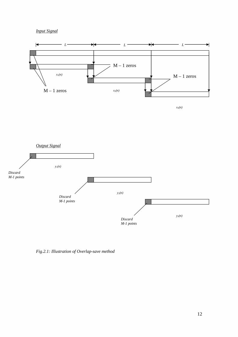
Input Signal

Output Signal

Fig.2.1: Illustration of Overlap-save method

y1(n)

y2(n)

y3(n)

Discard M-1 points

Discard M-1 points

Discard M-1 points

x1(n)

x2(n)

x3(n)

L L L

M – 1 zeros

M – 1 zeros

M – 1 zeros

12

2.2.2 Overlap add method

To each data block we append M – 1 zeros and computes the N point DFT. Thus the

IDFT yields data blocks of length N that are free of aliasing since the size of the DFT

and IDFT is N = L + M – 1, the sequences are increased to N point by appending

zeros to each block.

To concatenate the signal back to the original length , each last N – 1 points from each

output block must be overlapped and added to the M – 1 points of the succeeding

block, since each data block is terminated with M – 1 zeros [6]. Hence the name of

this method, Overlap add. Fig.2.2 depicts an illustration.

13

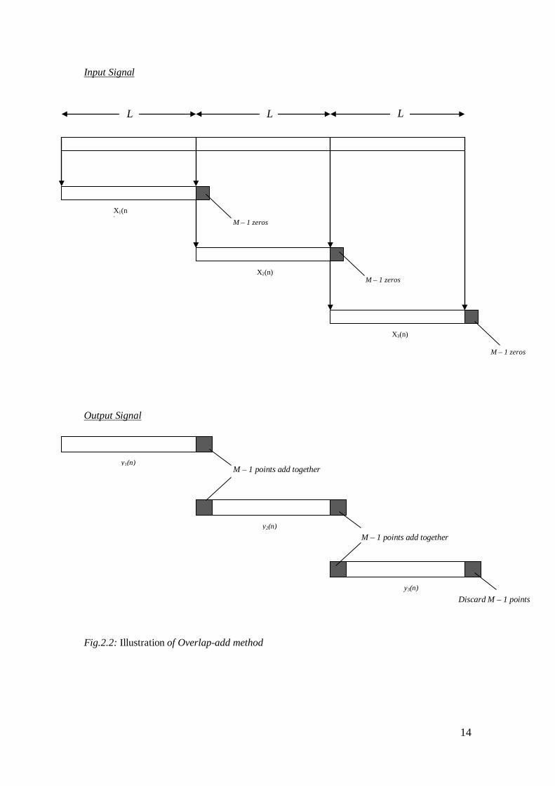
Input Signal

Output Signal

Fig.2.2: Illustration of Overlap-add method

M – 1 zeros

M – 1 zeros

M – 1 zeros

X1(n)

X2(n)

X3(n)

L L L

y1(n)

y2(n)

y3(n)

M – 1 points add together

M – 1 points add together

Discard M – 1 points

14

These two methods are commonly used to “cut” the signal in chunks and reconstruct

the signal after processing. The mathematical representation of Short Time Fourier

Transform (STFT) is written as:

( ) ( ) ( ) frjL

LrerwrxfX πττ 2, −

−=∑ −= (2.5)

where ss fLLfLf 1,1,0 −∈ is a frequency, w(r) is a window

that tapers smoothly to zero at each end and τ is the new index representing discrete

time.

Please note that the above equation is used when considering a discrete time signal,

but for a continuous time signal the Short Time Fourier Transform is written as;

( ) ( ) ( ) dtetwtxX tjωττ −∞

∞−−=Ω ∫, (2.6)

The graphical display of the magnitude of the Short Time Frequency

Transform ( )Ω,τX , is called the spectrogram of the signal. It is often used in speech

processing, also the output of the STFT is invertible and that is the reason why the

original signal can be recovered from it.

15

16

Chapter3

3.1 Optimization Methods

One of our major task in this project is to use ICA to find the separating matrix which

will be use to estimate the independent components. The separating matrix cannot be

written as some function of received samples, whose value could be directly solved,

instead the solution is based on cost functions also know as objective functions or

contrast functions. The solutions of the separating matrix are found at the maxima or

minima of these functions.

Optimization theory includes the study of the maximal and/or minimal values of a

function, and the conditions for the existence of a unique maximal or minimal value.

An example of an optimization problem is that of finding the minimum of a scalar

function or objective function and where the minimum is located. Assuming that this

objective function say g(x) is differentiable, the conditions for finding a local and

global minimum are:

• ( ) 0=dx

xdg (3.1)

• ( ) 02

2

>dx

xgd (3.2)

It’s important to note that these conditions must be fulfilled in order to define a

stationary point as a local minima, because without the second condition, fulfilment of

the first condition could be either a maxima, a minima or even an inflection point.

Stationary point refers to solutions of objective function that satisfied the first

equation, but to find the Global minimum; that is, value or values where the function

achieves its smallest value; the objective function must be evaluated at each stationary

point and the smallest is selected.

In a case where the objective function g(x) can be shown to be strictly convex there is

at most one solution to the equation (3.1) and this solution corresponds to the global

minimum of g(x). A function g(x) is strictly convex over a closed interval [a, b] if, for

any two points x1 and x2 in [a, b] and for any scalar α such that 10 ≤≤ α then

17

( )( ) ( ) ( ) ( )2121 11 xfxfxxf αααα −+<−+ (3.3)

When the objective function depends on a complex variable say z and it is

differentiable ( i.e. analytic) then finding the stationary points of g(x) is the same as in

the real case; find the derivatives, set it to zero and then solve for the locations of the

extrema (i.e. maximals and minimals). Of particular interest is when the function is

not differentiable, unfortunately in contrast to functions of real variable, many of the

functions that we want to minimized are not differentiable. A very good and common

example is the simple function g(z) 2z= . Although it is clear that g(z) has a unique

minimum that occurs at z = 0, this function is not differentiable [2].

The problem is that g(z) *2 zzz == is a function of z and z*(conjugate) and any

function that depends on the complex conjugate z* is not differentiable with respect to

z. The complication can be resolved with either of two methods; the first is to express

the objective function in terms of the real and imaginary parts z = x +jy and minimize

g(x, y) with respect to those two variables.

This approach is unnecessarily tedious but will yield the solution. A more elegant

solution is to treat z and z* as independent variables and minimize g(z, z*) with

respect to both z and z*. For example, if we write g(z) 2z= as g(z, z*) = zz* and

treat g(z,z*) as a function of z and keep z* constant then,

( ) *zdz

zdg= (3.4)

Where as if we treat g(z, z*) as a function of z* with z constant, then we have

( ) zdz

zdg=

* (3.5)

Setting both derivatives equal to zero and solving this pair of equations we see that

the solution is z = 0. [2]

3.1.1 Vector Gradients

Another situation is when the objective function depends on a vector–valued quantity

x the evaluation of the function’s stationary points is a simple extension of the scalar-

18

variable case. For a scalar function of m real variables f(x) = (x1, x2,. . .. xm), assuming

that the function is differentiable, this involves computing the gradient, which is the

vector of partial derivatives defined by

( )

( )

∂∂

∂∂

=∂∂

mxxf

xxf

f

1

x (3.6)

The gradient point is the direction of the maximum rate of change of f(x) and it is

equal to zero at the stationary points of f(x). Hence the aforementioned condition for a

point x to be a stationary point of f(x) must be satisfied, which is

( ) 0=dx

df x (3.7)

For this stationary point to be the minimum the Hessian matrix Hx must be positive

definite i.e.

XHHxX 0 for all x

The Hessian matrix is the second-order gradient of a function, in other words second-

order derivatives with (i,j)th element as

∂∂

∂∂

∂∂

∂∂

=∂∂

2

2

1

2

1

2

21

2

2

2

mm

m

xf

xxf

xxf

xf

f

x (3.8)

If f(x) is strictly convex, then the solution is unique and is equal to the global

minimum.

19

It’s is easy to see that the Hessian matrix is always symmetric. The Jacobian matrix,

of f(x) with respect to x which we will later use is given by:

∂∂

∂∂

∂∂

∂∂

=∂∂

m

n

m xf

xf

xf

xf

f

1

1

1

1

1

x (3.9)

Thus the ith column of the Jacobian matrix is the gradient vector of fi(x) with respect

to x.

3.1.2 Matrix gradient

Assuming we have a scalar valued function g of the elements of an m x n matrix W

in analogy with the vector gradient, the matrix gradient means a matrix of same size

m x n as the matrix W, whose ijth element is the partial derivative of g. We can write it

as:

∂∂

∂∂

∂∂

∂∂

=∂∂

nm

m

wg

wng

wg

wg

g

1

111

W (3.10)

3.2 Learning Rules for Optimization

Let us look at the rules (or algorithms) of finding the extrema points of a cost

function. Although the vector that minimizes the cost function may be found by

setting the derivatives of the cost function equal to zero as earlier said, another

approach is to search for the solution. There are many search method and we are

going to point out few.

20

3.2.1 Gradient descent

This is an iterative procedure that has been used to find the extrema values of

functions long since before the time of Newton. Let us consider in more detail the

case when the solution is a vector w; the matrix case goes through in the same way.

The basic idea behind this method is that we minimize the cost function say ζ(w) by

starting from some initial point value w(0), then computing the gradient of ζ(w)at this

point and moving in the direction of the negative gradient or the steepest descent by a

suitable distance. This procedure is repeated at the new point, this is continued until it

converges, which in practice happens when the Euclidean distance between two

consecutive solutions, that is ( ) ( )1−− tt ww goes below some small tolerance level.

Thus the learning rule update is

( ) ( ) ( ) ( )wwww

∂∂

−−=ζα ttt 1 (3.11)

With the gradient taken at the point w(t – 1), while the parameter α(t) often refers to

the step size, or the learning rate, gives the length of the step in the steepest descent

which always point in the negative gradient.

Geographically we can view the graph of the function ζ(w) as equivalent of mountain

terrain, so the gradient descent learning rule means that we are always going down the

hill in the steepest direction.

The major disadvantage of this method is that it always leads to the closest local

minimum instead of a global minimum, unless the function ζ(w) is strictly convex.

That is when we have one local minimum which is also the global minimum. Non-

quadratic functions may have many local minimal values; therefore good initial

values are important in initializing the algorithm [5]. It’s important to also note that

the choice of an appropriate learning rate is essential, because too small a value will

lead to slow convergence while too large a value will lead to overshooting and

instability which prevents convergence altogether.

21

For better understanding of the idea, let us assume that the contour plot of the cost

function ζ(w) is as shown in Fig. 3.1

Fig.3.1: Contour map of assumed cost function.

From the illustration we can see there are three extrema, two local minima and one

global minimal. If we choose our initial value in the direction of the gradient vector,

we will surely end up with one of the local minimum, which is not the optimal

solution. Base on this it’s important to be very careful when choosing our initial

values say w(0) as earlier mentioned.

3.2.2 Natural Gradient

We saw the disadvantage of Gradient descent; unless the cost function is quadratic, it

may not lead to the global minimum in non-quadratic function which may have more

than one extrema. As earlier said, it points in the opposite direction of the gradient in

an Euclidean orthogonal coordinate system. Orthogonal mean that the coordinates are

perpendicular to each other.

Local minimum

Local minimum

Global minimum

Gradient vector direction

Current position

22

Amari reports in [13,14], that parameter space is not always Euclidean but also has

Riemannian metric structure. In this case the Gradient descent does not give the

steepest direction of the target function; instead the steepest direction is given by the

Natural gradient. Since we are mostly concerned with ICA learning rules, we will

constrain ourselves to the case of nonsingular matrix also know as invertible matrix

(i.e. matrices with existing inverse) which are very important to ICA. Amari also

added that these matrices (i.e. nonsingular) have a Riemannian structure with a

convenient computable natural gradient.

Let’s assume that the function is ζ and W∂ be a small deviation or minimization of a

matrix from W to W + W∂ , under the constraint that the square norm 2W∂ is a

constant.

One of the major requirements is that at any step in gradient algorithm for

minimization of a function, there must be a direction of the step and the length of the

step. Keeping this length constant the optimal direction is search for [8].

Introducing an inner product at W by defining the square norm of W∂ as:

W

WWW ∂∂=∂ ,2 (3.12)

And by multiplying W-1 from right, we mapped W to WW-1 = I i.e. identity matrix

and W + W∂ is mapped to

(W + W∂ )W-1 = I + W∂ W-1 = I + X∂ . (3.13)

where X∂ = W∂ W-1.

It means that a deviation W∂ at W is equivalent to a deviation X∂ at I.

Amari argues that due to the Riemannian structure of the matrix space, it requires that

metric is kept invariant, that is, the inner product of W∂ at W is equal to the inner

product of WZ∂ at WZ for any Z.

WZW

WZWZWW ∂∂=∂∂ ,, (3.14)

Putting Z = W-1 then WZ = I and if the inner product at I is define as

( ) ( )WWWWWI

∂∂=∂=∂∂ ∑ Tm

ji ji trace,

2,, (3.15)

then equation (3.14) can de deduced to

( )( )1111 ,, −−−− ∂∂=∂∂=∂∂ WWWWWWWWWWI

TTW

trace (3.16)

23

Amari finally shows that keeping this inner product constant, the largest increment for

ζ(W + W∂ ) is obtained in the direction of the natural gradient which is

WWWW

T

nat ∂∂

=∂∂ ζζ (3.17)

It then means that the usual Gradient descent at point W must be multiplied from right

by the matrix WTW and this gives the Natural Gradient learning rule update at point

W(t) as follows:

( ) ( ) ( ) WWW

WW Tttt∂∂

−−=ζα1 (3.18)

Amari pointed out that Natural Gradient learning rule is fisher efficient, implying that

it has asymptotically the same performance as the optimal batch estimation of

parameters. Natural Gradient can be used in many applications like statistical

estimation of probability density function, multilayer neural network, blind signal

deconvolution, blind signal separation, etc and it is the algorithm we used.

24

Chapter 4

4.1 Blind Source Separation

Blind source separation (BSS), is a technique for estimating individual source

components from their mixtures at sensors. This is called blind because, the

estimation is done without prior information on the sources, that is their spatial

location and time activity distribution; and on the mixing function, i.e. information

about the mixing process. The problem has become increasingly important in the area

of signal and speech processing due to their prospective application in speech

recognition, teleconferencing, hearing aids, telecommunications and medical signal

processing, etc. In these applications, signals are mixed in a convolutive manner, at

times with reverberation otherwise literary called echo. This makes blind source

separation a very difficult problem. Very long Finite Impulse Response (FIR) filters

of several thousand taps will be needed to separate acoustic signals mixed in such

manner. [1]

Many scholars and researchers have been studying the problem of Blind Signal

Separation and numerous ways have been proposed to solve the problem. Recently

attention has been drawn to Independent Component Analysis (ICA), which is a very

important statistical tool for solving the BSS problem.

As earlier said, the aforementioned applications involve convolutive mixtures of the

sources. If they were mixed instantaneously, without any delay, solving the problem

with ICA would have been far much easier. We would have just applied instantaneous

ICA and that would separate the sources (this will be shown later) although with the

problem of scaling and permutation ambiguities.

Due to filtering imposed on sources by their environments, difference between the

sensors and propagation delays, what we always observe in real world applications

like the aforementioned applications are convolved signal. We need to extend the

Blind Source Separation using Independent Components Analysis technique so that it

will be applicable to the convolutive mixtures. There are three major approaches of

solving the convolutive mixtures using ICA/BSS as enumerated in [1] by Makino et

al, which all have some advantages and disadvantages.

25

First is the Time domain BSS, where ICA is directly applied to the convolutive

mixtures. This achieves a good result once the algorithm converges, but it is

computationally expensive because we are dealing with convolution operations.

The second is the Frequency domain BSS, where the convolutive mixtures are first

converted to Frequency domain, then ICA is applied to each frequency bin, which is

seen now as instantaneous mixtures, since convolution in time domain is equal to

multiplication in frequency domain. This method is simple but the problem of

permutation and scaling is even greater than in the Time domain BSS since different

frequency bands may have different permutation and scaling.

The third approach uses both the time domain and frequency domain. Here the filter

coefficients are updated in the frequency domain, but the nonlinear functions for

evaluating independence are applied in the time domain. This approach does not have

the permutation problem, because the independence of the separated signals are

evaluated in time domain, but the time spent in switching between the time domain

and the frequency domain is non negligible. [19]

From these three approaches, the second is better in terms of computational demand,

but the problem of permutation and scaling has to be resolve as earlier mentioned.

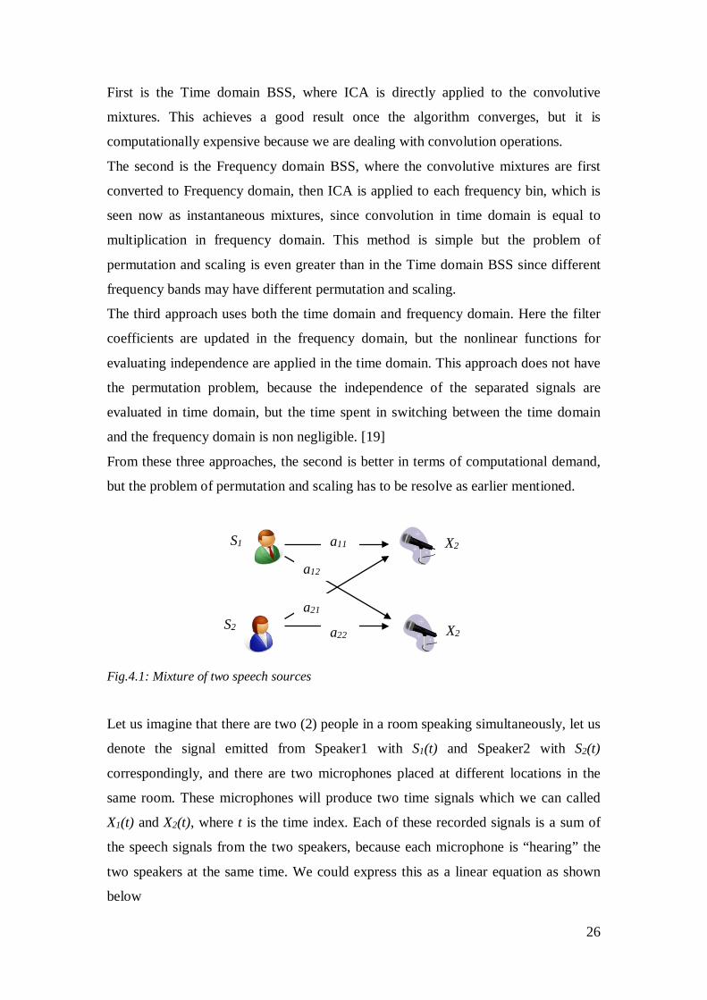
Fig.4.1: Mixture of two speech sources

Let us imagine that there are two (2) people in a room speaking simultaneously, let us

denote the signal emitted from Speaker1 with S1(t) and Speaker2 with S2(t)

correspondingly, and there are two microphones placed at different locations in the

same room. These microphones will produce two time signals which we can called

X1(t) and X2(t), where t is the time index. Each of these recorded signals is a sum of

the speech signals from the two speakers, because each microphone is “hearing” the

two speakers at the same time. We could express this as a linear equation as shown

below

S1

S2

a11

a12

a22

a21

X2

X2

26

( ) 2121111 SaSatX ⊗+⊗=

( ) 2221212 SaSatX ⊗+⊗= (4.1)

Where ⊗ represents convolution, aij are some parameters that depend on the

distances of the microphones from the speakers and on the room properties, these

parameters are referred to as the room impulse response.

This scenario is normally refer to as the cocktail-party problem, it would be very

useful if the original speech signals S1(t) and S2(t) could be estimated. What it then

means is that if we knew the values of a11, a12, a21 and a22 (i.e. the impulse response)

we could easily solve the linear equation above with any of the classical methods

available, but not knowing these values is the main problem and even make it a

difficult one. Independent Component Analysis (ICA) can be used to estimate these

values and allow us to separate the two original signals S1(t) and S2(t) from their

mixtures X1(t) and X2(t).

( )

( )

( ) ( )

( ) ( )

( )

( )

( ) ( )

( ) ( )

( )

( )

→

→

→

→

ty

ty

lwlw

lwlw

tx

tx

lala

lala

ts

ts

N

NMN

M

M

MNM

N

N

1

1

111

1

1

111

1

Fig.4.2: The schematic diagram of BSS for Convolutive Mixtures

The above diagram shows how the blind source separation for convolutive mixtures

can be formulated. Assuming we have N source signal si(t) that are mixed and

observed at M sensors as xj(t), thus mathematically we can write:

( ) ( ) ( )11

−= ∑ ∑=tslhtx i

N

i l jij j = 1,. ….. , M (4.2)

Where j,i represent the impulse response from source i to sensor j.

It’s always assumed that the number of sources N is known or can be estimated and

the number of sensors M is equal to or greater than N; NM ≥ . The mixed signal X is

27

passed through the separation system which consists of finite impulse response (FIR)

filters wij(l) of length l to produce N separated signals yi(t) as the output. Thus;

( ) ( ) ( )ltxlwty jM

j

L

l iji −= ∑ ∑=

−

=1

1

0 i = 1,. . . . . ,N (4.3)

The separation filters, wij(l) should be estimated blindly, i.e., without any knowledge

of the source signal si(t) or hji(t) the mixing function.

4.2 Independent Component Analysis

Independent Component Analysis is a powerful higher order statistical technique used

to separate independent sources that were linearly mixed together through a medium

and received at several sensors.

Let us assume that we observe N linear mixtures x(t)1, x(t)2, ………x(t)N of M

independent components.

NjNjjj sasasa +++= 2211x for j = 1,2,3……,M (4.4)

As earlier said in chapter 1, the number of sensors is usually greater than or equal to

the number of sources ( )NM ≥ .

In the general ICA model the time index is not used because we assumed that each

mixtures xj as well as independent components Sk are random variables instead of

proper signals [5].

It is convenient to use vector-matrix notation instead of the sums as shown above, let

x denote the random vector whose elements are the mixtures x1,……xM and let s

denote the random vector with elements s1,……..,sN. Let A denote the matrix with

elements aij.

The mixture model using the vector-matrix is written as x = As or graphically as

28

=

N

MNM

N

M s

s

aa

aa

x

x

1

1

111

1

(4.5)

This ICA model is a generative model because it describes how the observed data are

generated by a process of mixing the components sj. It’s important to recall that all we

observe and know is the random vector x and we estimate the inverse A and s using it

alone. This can’t be achieved without some general and fundamental assumptions

which are:

i) We assumed that the components sj (i.e. the sources) are statistically

independent between each other

ii) And that the Independent components must have non Gaussian

distribution (At most one source may have Gaussian distribution).

4.2.1 Statistical Independence

The concept of statistical independence can easily be explained with an example. Let

us assumed that y1 and y2 are scalar valued random variables, y1 and y2 are said to be

independent if the information of the value of y1 does not give any information of the

values of y2 and likewise, information of the values of y2 does not give any

information of y1. It’s important to note that we are referring this to the sources (si)

alone and not the mixtures (xi), which generally are highly dependent.

In probability theory, independence can be defined by the probability densities. Let

( )11 yP denote the Marginal Probability Density Function (i.e. the probability density

function when y1 is considered alone) and let ( )21 , yyP denote the Joint Probability

Function (i.e. considering y1 and y2 together).

Then

( ) ( ) 22111 , dyyyPyP ∫= (4.6)

Likewise

( ) ( ) 12122 , dyyyPyP ∫= (4.7)

29

We say y1 and y2 are independent if and only if the Joint Probability Density Function

can be factorised in the following way:

( ) ( ) ( )221121 , yPyPyyP = (4.8)

In other words two events are statistically independent if the probability of their

occurring jointly equals the product of their respective probabilities.

4.2.2 Nongaussian Distribution

Another fundamental restriction or assumption in ICA is that the independent

component must be nongaussian or at most may have one Gaussian distribution, for

Independent Component Analysis to be possible[5,7,8]; this is because of the joint

probability densities of Gaussian random variables are completely symmetric.

Moreover for Gaussian random variables mere uncorrelatedness implies

independencies and thus any decorrelating representation would give independent

components. Nevertheless if not more than one of the components are Gaussian it is

still possible to identify the nongaussian independent components as well as the

corresponding columns of the mixing matrix. In other words without nongaussianity,

estimation of the ICA model is not possible at all.

30

Fig.4.3: Plot of Probability Density Function of some Gaussian distributions. [10], μ is the mean and σ2is the variance.

4.3 Measures of Nongaussianity

Since nongaussianity is important in estimation of ICA models thus there is need for a

quantitative measure. Let us look at some measures of nongaussianity, their

advantages and disadvantages.

4.3.1 Kurtosis

Kurtosis is a parameter that describes the shape of a random variables’ probability

distribution function. It can also be used to measure nongaussianity of a random

variable, because a Gaussian distribution (which sometimes is refer to as normal

distribution) has a normalized kurtosis equal to zero, in other words Mesokurtic.

Since Gaussian distribution have normalized kurtosis equal to zero, it can be used as a

reference point to know distributions that are below Gaussian distribution

(subgaussian, they have negative kurtosis) in other words Platykurtic and those that

31

are above Gaussian distribution(supergaussian, these have positive kurtosis) otherwise

called Leptokurtic. A leptokurtic distribution has a more acute “spiky” shape around

zero, this means, a higher probability than a Gaussian distribution near the mean; and

a “long tail”; this entails a higher probability than a Gaussian distribution at the

extreme values. A good example of a leptokurtic distribution is the Laplace

distribution.

A platykurtic distribution has a “flatter peak” around mean, this implies a lower

probability than Gaussian distribution near the mean; and “small tail” (that is lower

probability than a Gaussian distribution at the extreme values. A typical example of a

platykurtic distribution is the Uniform Distribution.

Fig.4.4: Different well known distribution together with their kurtosis measure, D= Laplace Distribution, S=hyperbolic Secant Distribution, L= logistic Distribution, N= Normal Distribution, C= Raised Cosine Distribution, W=Wigner Semicircle Distribution, and U= Uniform Distribution [10].

32

Using statistical terms the Normalized Kurtosis of a standard variable y is defined by:

( )

322

4

−=yEyEykurt (4.9)

This shows that Kurtosis is simply a normalized version of the fourth moment Ey4.

Some properties of kurtosis are;

If x1 and x2 are two independent random variables, then

( ) ( ) ( )2121 xkurtxkurtxxkurt +=+ (4.10)

and

( ) ( )12

1 xkurtxkurt αα = (4.11)

The simplicity both in computation and theory of these properties makes kurtosis

widely used to measure nongaussianity in ICA but, it has some drawbacks in practice,

when its value has to be estimated from a measured sample. Its major hindrance is

that kurtosis can be very sensitive to “far away” data; its value may depend on only a

few observations in the “tail” of a distribution which may be erroneous or irrelevant

data. This makes kurtosis not a robust measure of nongaussianity [5].

4.3.2 Negentropy

Another important measure of nongaussianity is Negentropy. It is a short word for

“Negative Entropy” which from its name, is based on Entropy. To continue with

negentropy it is important to understand the meaning of Entropy, which is a basic

concept in information theory.

Entropy of a random variable as defined by [5] can be interpreted as the degree of

information that an observation of a random variable gives. It is a measure of the

uncertainty associated with random variables, in other words the more random,

unpredictable and unstructured the variable is, the larger its entropy.

The entropy of a discrete random variable x is defined as:

( ) ( ) ( ) ( )( )xIEayPaxPxH xin

i i ===−= ∑ = 21log (4.12)

Where ai is the possible values of x

I(x) is the information content or self – information of x which is itself a

random variable

P(x = ai ),P(y = ai) is the probability density function.

33

This definition can also be extended to the continuous random variable; in this case

it’s often referred as Differential Entropy. Assuming we have a continuous random

variable y, the differential entropy is written as;

( ) ( ) ( )dyyfyfyH 2log∫−= (4.13)

where f(y) is the probability density function of y.

One of the fundamental rule of thumb in information theory is that a Gaussian

Variable has very large entropy among all random variables of equal variance. This

means that Gaussian distribution is very random, disorganised and unstructured

distribution and this implies that entropy can be used to measure nongaussianity.

So, to measure a nongaussianity of a variable that will give us zero for a Gaussian

variable and non negative for nongaussian variable, we use Negentropy which can be

defined for a standard variable y as:

( ) ( ) ( )yHyHyJ gauss −= (4.14)

where ygauss is a Gaussian variable of the same covariance matrix as y.

Negentropy is a very good measure of nongaussianity, but not with a setback which is

difficulty in computation. Estimating negentropy requires an estimate of the

probability density function, so simple approximations of negentropy are very helpful.

A well known computational and simple approximation of entropy of a standardised

(i.e. zero mean and unit variance) random variable is

( ) ( )223

481

121 ykurtyEyJ += (4.15)

Now, since we assumed that the random variable is standardised, that is zero mean

and unit variance, the first term on the right hand side of the above equation is equal

to zero when the random variable has a symmetric distribution which is often the

case. Then this approximation will be equal to square of the Kurtosis, thereby putting

us in the same problem as mention in the last subsection, which is non-robustness of

measure of nongaussianity.

Another approach described in [5] is based on the maximum – entropy principle, here

the higher order approximation is replaced with the expectation of general non-

quadratic functions or “non-polynomial moments”. The polynomial function y3 and y2

34

can be replaced by any other functions Gi (where i is an index not exponent), the

method then gives a simple way of approximating the negentropy based on the

expectation EGi [5]. So, the new approximation the becomes

( ) ( ) ( ) [ ]2vGEyGEyJ −≈ (4.16)

for one quadratic function G,

where v is a Gaussian variable of zero mean and unit variance.

Now, in choosing the function G one has to be careful so as to:

1. get an approximation better than (4.15)

2. not to get a kurtosis based approximation.

Therefore choosing G we need to be sure that practical estimation of EGi(y) should

not be practically difficult and should not be too sensitive to the outliers (outliers is a

statistical terms for extreme values of data). Secondly G(y) must not grow faster than

the quadratic function of y i.e. y2.

The choices of G that have proved very useful according to [5,7,8] are:

• ( ) ( )yaa

yG 11

1 coshlog1= (4.17)

• ( )

−−= 2exp

2

2yyG (4.18)

Where 21 ≤≤ a is a suitable constant, often taken equal to one, this gives a very

good compromise between kurtosis and Negentropy [5,7,8].

4.4 Maximum Likelihood Method

In order to understand ICA by Maximum likelihood (ML), it is important to

understand some basic terms in Estimation Theory which maximum likelihood

belongs to.

Estimation theory aims at extracting from noise corrupted observations, information

or data of interest. Assuming that there are t scalar measurements say

x(1), x(2), . . . . . . . , x(t) containing information about n quantities that we which to

estimate say u1, u2, . . . . . . . . ,un. These quantities ui are called parameters, they can

be represented as a vector u = [u1, u2, . . . . . . . . ,un]T, so also the measurements

35

x = [x(1), x(2), . . . . . . . , x(t)]T, where T means transpose of the vector.

Generally, the estimator of the parameter vector, represented as Û, is a vector function

by which the parameters can be estimated from the measurements, so mathematically

we can write it as:

( ) ( ) ( ) ( )( )txxxfxfU n ,2,1ˆ == (4.19)

Or individually we can write it as:

( )zii xfu =ˆ (4.20)

The numerical value of an estimator ûi is called the estimate of ui.

There are numerous examples of estimators like method of moments, least squares,

Bayes, maximum likelihood, to name but a few but here we are dealing with

maximum likelihood.

Maximum likelihood estimator assumes that the priori information or density of the

distribution is known or assumed known. It has some asymptotic (asymptotic in the

sense that the more the variables the better the result) optimal properties (which are

its consistency and efficiency) that makes it a robust and desirable choice of

estimation. The maximum likelihood estimate of a parameter U (represented as ÛML)

is the value of the estimate that maximizes the likelihood function of the measurement

just as its name implies.

The likelihood function, which can be likened to the joint probability function of the

measurements assuming that the measurements are independent, is given as:

L(x(1), x(2), ... , x(t)u1, u2, ... ,un) = ( )( )∏ ==

t

i nuuuixPL1 21 ,,,; (4.21)

Taking the logarithm of the above equation we have

( )∑ ==

t

i ni uuuxPL1 21 ,,;lnln (4.22)

Maximum likelihood estimates are obtained by maximizing L or lnL, by maximizing

lnL which is much easier than L, the maximum likelihood estimate of U are the

simultaneous solutions of n equations such that:

0ln=

∂∂

iuL for j = 1,2, . . . ., n (4.23)

Now, that we have a little background knowledge of maximum likelihood estimates,

in order to derive the ICA algorithm using maximum likelihood estimator we also

36

need to have a review of the probability density caused by a linear transform to a

standard variable.

4.4.1 Probability Density Function of a Transformed Variable

Assuming we have 2 random variables X and S of n dimensional, that are related as

follows:

X = AS (4.24)

for which the inverse

S = A-1X (4.25)

exist and is unique, then the probability density Px(X) of X can be obtained from the

Probability Density Function (PDF) Ps(S) of S as shown below:

( )( )( ) ( )( )XAPXAJ

XP sg

x1

1det1 −

−= (4.26)

Where Jg is the Jacobian matrix, that is:

( )

( ) ( )

( ) ( )

∂∂

∂∂

∂∂

∂∂

=

n

n

n

n

g

xXg

xXg

xXg

xXg

XJ

1

11

1

Since the transformation X = AS is linear and nonsingular, then the equation (4.26)

can be reduced to:

( ) ( )( )XAPA

XP sx1

det1 −= (4.27)

4.4.2 The Maximum Likelihood of ICA Model

Based on equation (4.27) above which is the PDF of a linear transformation and being

aware of our ICA generative model

x = As

37

The PDF of the mixture vector x, Px can be written as:

( ) ( )sCx sx PP det= (4.28)

This can also be written as:

( ) ( )iix sPP ∏= ˆdet Cx (4.29)

Where C = A-1 since A is nonsingular, Pi denotes the densities of the independent

components. Recalling that s = A-1x = Cx, we can write equation (4.29) as follows:

( ) ( )xCx Tiix cPP ∏= ˆdet (4.30)

Assuming x are N observations which of course are statistically independent of each

other, then the likelihood denoted by L (please note that at this juncture that we need

to find the likelihood on which we base the calculation of the Maximum likelihood)

can be obtained as the product of these densities evaluated at the N points. This is

evaluated as a function of C

( ) ( )( )∏ ∏==

N

j

n

iTii jxcPL

1detln CC (4.31)

As earlier said it is easier and more practical to use the logarithm of the likelihood,

based on this we can rewrite equation (4.31) as

( ) ( )( ) CC detlnlnln ∑ ∑ +=N

j

n

iTi NjxcPL (4.32)

It is important to note that taking logarithm of likelihood does not make any

difference in the location of the optimum value, since the maximum of logarithm,

lnL(C) is obtained at the same point as the maximum of the L(C). The base of the

logarithm does not make any difference although natural logarithm is preferred.

Equation (4.32) can further reduced as follows

( ) ( ) CC detlnln1+= ∑n

iTii xcPML

N (4.33)

Where M is an average computed from the observed sample i.e. mean over N

samples.

38

Performing maximum likelihood estimation in practice, we need an algorithm to

perform the numerical maximization of the likelihood function, from (chapter 3), the

gradient of the log likelihood function in equation (4.33) can be written as:

( )[ ] ( ) TT gLT

xCxCC

+=∂∂ −1ln1 (4.34)

Or in the gradient descent learning rule form:

( ) ( ) ( ) ( )( )TT gtt xCxCWW +−−=−11 α (4.35)

The Natural gradient method simplifies the maximization of the likelihood and it

makes it better conditioned. To derive the natural gradient ICA algorithm we multiply

the second part of the above equation (4.35) by the matrix CTC from right just as

earlier shown in the optimization chapter, thus we have:

( ) ( ) ( ) ( )( )( )CCxCxCWW TTT gtt +−−=−11 α (4.36)

and this reduces to

( ) ( ) ( )( )( )CssIWW Tgtt +−−= α1 (4.37)

But we still have a problem and that is the density distribution of the independent

components which we don’t know but we have to assume a model. Since we know

that speech signals have a distribution close to Laplacian distribution and that the

derivative of tanh function is close to it, we may choose that:

g(s) = tanh(s) (4.38)

If we write that

( )( )

( )sss

ss

s

P

P

g ∂∂

−= (4.39)

where

s∂

∂=

gP (4.40)

39

then

( ) ( ) ( )2tanh1tanh ss

ss −=∂

∂=sP (4.41)

( ) ( ) ( ) ( )( )2

2

2

tanh1tanh2tanh sss

sss

−−=∂

∂=

∂∂ sP

(4.42)

( ) ( )( )( )( ) ( )ss

ss tanh2tanh1

tanh1tanh22

2

=−

−−=g (4.43)

At the optimum C = W and we use W(t-1) as C, so ICA Natural gradient learning rule

update is shown below as

( ) ( )[ ] ( )1tanh21 −−−−= tt T WssIWW α (4.44)

Please note that the constant 2 may be removed when using the update rule. Thus the

resulting algorithm is recapitulated as

ICA Natural Algorithm

Given M mixed signals x(1), x(2), . . . . . . . , x(m) of length L

• Step 1: Initiate W to the identity matrix(m x m)

set m = 1

• Step 2 : Calculate the output s(m) that is the independent components,

s(m) = Wx(m)

• Step 3 : Update W as ( ) ( )[ ] ( )1tanh21 −−−−= tt T WssIWW α until

convergence.

40

Chapter 5

5.1 Frequency Domain Convolutive BSS/ICA

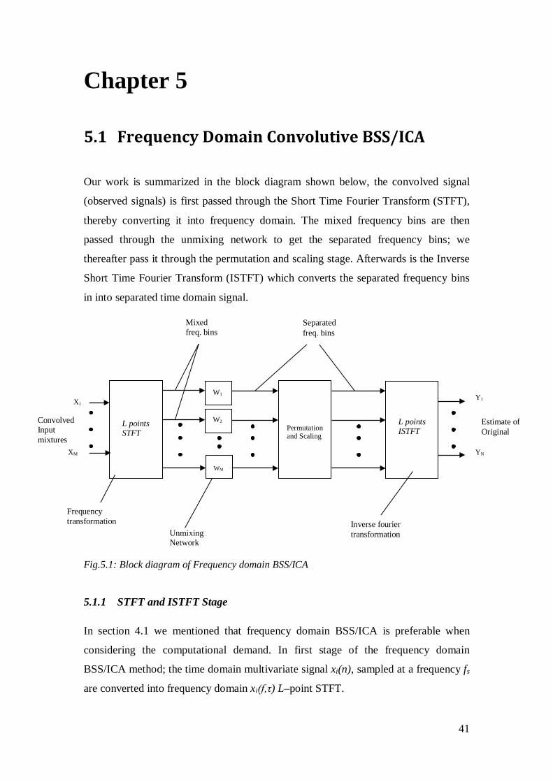
Our work is summarized in the block diagram shown below, the convolved signal

(observed signals) is first passed through the Short Time Fourier Transform (STFT),

thereby converting it into frequency domain. The mixed frequency bins are then

passed through the unmixing network to get the separated frequency bins; we

thereafter pass it through the permutation and scaling stage. Afterwards is the Inverse

Short Time Fourier Transform (ISTFT) which converts the separated frequency bins

in into separated time domain signal.

Fig.5.1: Block diagram of Frequency domain BSS/ICA

5.1.1 STFT and ISTFT Stage

In section 4.1 we mentioned that frequency domain BSS/ICA is preferable when

considering the computational demand. In first stage of the frequency domain

BSS/ICA method; the time domain multivariate signal xi(n), sampled at a frequency fs

are converted into frequency domain xi(f,τ) L–point STFT.

WM

Permutation and Scaling

L points STFT

Convolved Input mixtures

Frequency transformation

Unmixing Network

X1

XM

Mixed freq. bins

W1

W2 L points ISTFT

Inverse fourier transformation

Separated freq. bins

Estimate of Original

Y1

YN

WM

41

( ) ( ) ( ) frjL

Lrjj erwinrxfx πττ 22

2

, −

−=∑ += (5.1)

where ss fLLfLf 1,,1,0 −∈ is a frequency, win(r) is a window that tapers

smoothly to zero at each end and τ is the new index representing time. Note that in the

equation (5.1) the length L is divided by 2, this is because in Fourier transformation

half of the length of the transformation is repeated and flipped. So what we have in

the second half of L is the mirror image of the first half.

So, the problem is converted into the task of demixing an instantaneous mixture at

each frequency bin,

( ) ( ) ( )ττ ,,1

fsfhjifx iN

ij ∑== (5.2)

Where hji(f) is the frequency response from source i to sensor j and si(f,τ) is the

frequency domain time series signal of si(t) obtained by using same L point short time

Fourier transform. The equation above can be rewritten using vector notation thus,

( ) ( ) ( )∑ ==

N

i ii fsffx1

,, ττ h (5.3)

Where x = [x1, x2, . . .. . , xM]T is the vector of mixed samples and

hi = [h1i, . . . . ., hMi]T is the vector of the frequency response from source si to all M

sensors.

In our work we use the recorded signal available from [17], it was recorded with two

talking microphones (sampled at 16kHz) in a normal office room with a loud music in

the background. The distance between the speaker, cassette player and the

microphones is about 60cm in a square constellation.

We wrote short time Fourier transform and inverse short time Fourier transform

programs in Matlab and to be sure that these programs were working correctly, we ran

them on a sinusoidal signal with a frequency of 2kHz, sampled at 10kHz frequency.

The power spectrum of the signal was estimated before short time Fourier transform

as show in the Fig. 5.2 below;

42

Fig.5.2: The Power Spectral Density of the sinusoidal signal before STFT

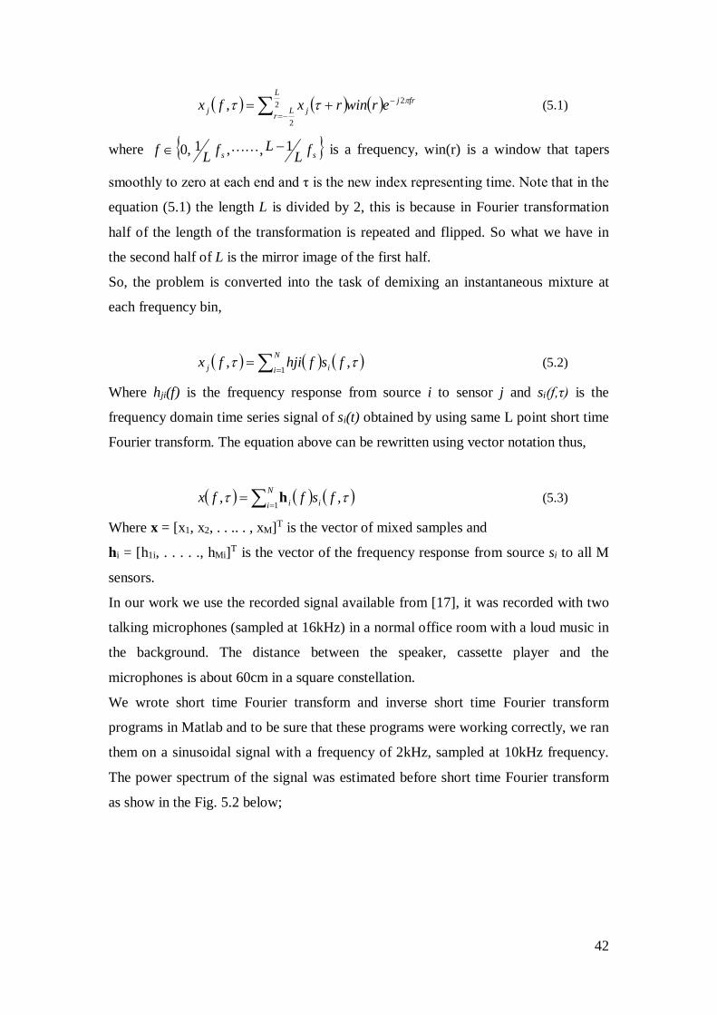
After STFT and consequently ISTFT the power spectrum of the output was also

estimated as shown in Fig.5.3 below.

43

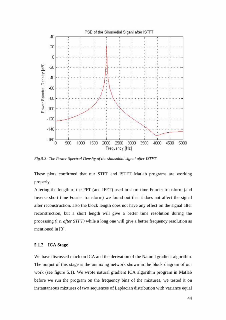
Fig.5.3: The Power Spectral Density of the sinusoidal signal after ISTFT

These plots confirmed that our STFT and ISTFT Matlab programs are working

properly.

Altering the length of the FFT (and IFFT) used in short time Fourier transform (and

Inverse short time Fourier transform) we found out that it does not affect the signal

after reconstruction, also the block length does not have any effect on the signal after

reconstruction, but a short length will give a better time resolution during the

processing (i.e. after STFT) while a long one will give a better frequency resolution as

mentioned in [3].

5.1.2 ICA Stage

We have discussed much on ICA and the derivation of the Natural gradient algorithm.

The output of this stage is the unmixing network shown in the block diagram of our

work (see figure 5.1). We wrote natural gradient ICA algorithm program in Matlab

before we run the program on the frequency bins of the mixtures, we tested it on

instantaneous mixtures of two sequences of Laplacian distribution with variance equal

44

to two, zero mean and the length equal to ten thousand. The mixing matrix A is a 2-

by-2 matrix with a full rank (i.e. the matrix is invertible).

We check the performance of ICA separation by plotting the condition (the condition

number of a matrix is a measure of stability or sensitivity of a matrix to numerical

operations, matrices with condition number near one is said to be well conditioned)

of the performance matrix during training. The performance matrix,

AWP ×=

where W is the separation matrix, should be equal to a, possibly rescaled and

permutated identity matrix. It then means that the condition number of the

performance matrix should tend towards one during the training.

The plot of the condition number is show in Fig.5.6 below;

Fig.5.5: The plot of the condition of a performance matrix.

45

Fig 5.5 above confirmed that our natural gradient ICA algorithm program is working

in order.

Since we are using the hyperbolic tangent as our cost function in the ICA algorithm as

earlier said in the previous chapter, we have to consider that the outputs of the STFT

(that is the Fourier Transform) are complex variables. In [11] it is showed that due to

the singularities at these points , for k = 0, 1, . . . . ., the hyperbolic tangent

is undefined.

This will introduce numerical problems and seriously hinder convergence (See Fig.5.7

below).

Fig.5.6: The plot of hyperbolic tangent of complex number [11]

He argued that it’s better to use hyperbolic tangent separately on the real and

imaginary parts of the complex variables as

. (5.4)

46

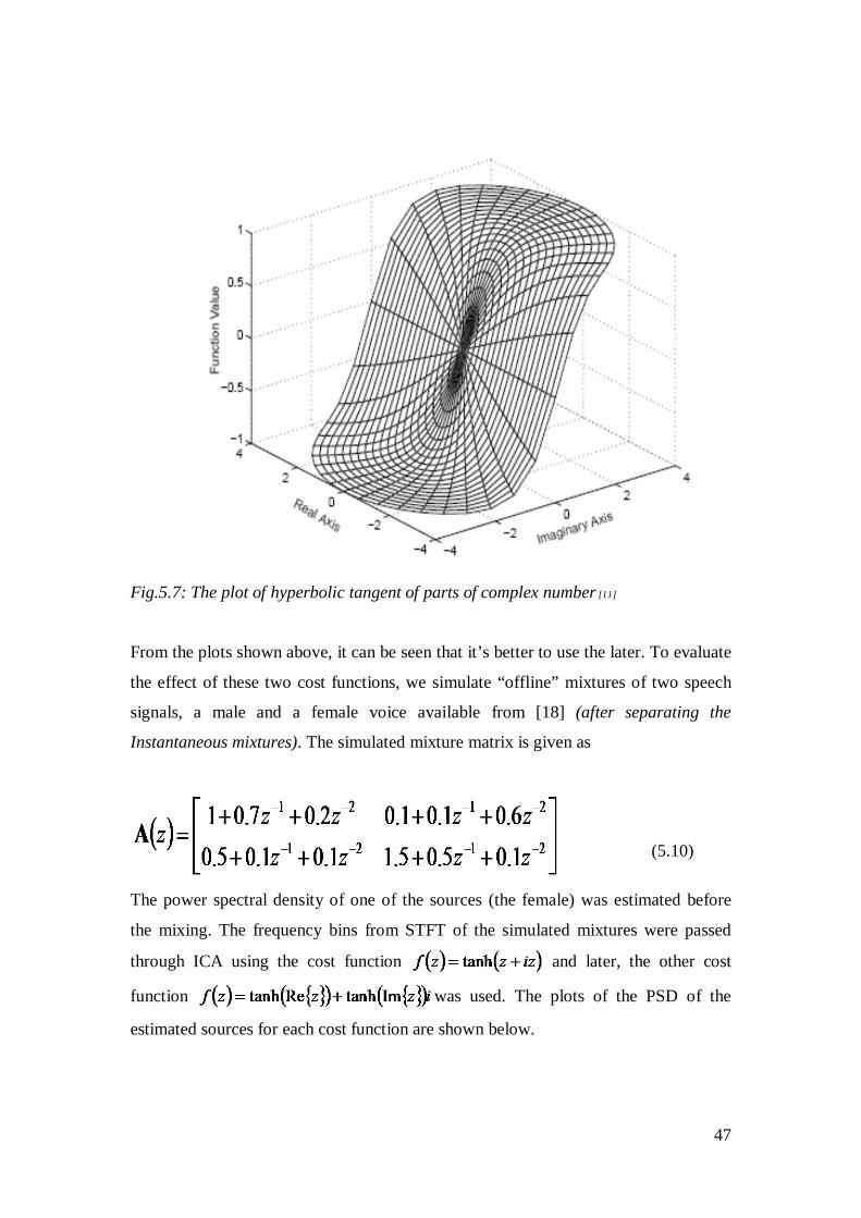
Fig.5.7: The plot of hyperbolic tangent of parts of complex number [11]

From the plots shown above, it can be seen that it’s better to use the later. To evaluate

the effect of these two cost functions, we simulate “offline” mixtures of two speech

signals, a male and a female voice available from [18] (after separating the

Instantaneous mixtures). The simulated mixture matrix is given as

(5.10)

The power spectral density of one of the sources (the female) was estimated before

the mixing. The frequency bins from STFT of the simulated mixtures were passed

through ICA using the cost function and later, the other cost

function was used. The plots of the PSD of the

estimated sources for each cost function are shown below.

47

Fig.5.8: The plot of the source and estimated source using ( ) ( )izzzf += tanh as ICA cost

function.

Fig.5.9: The plot of the source and estimated source using

( ) ( ) ( )izzzf ImtanhRetanh += as ICA cost function.

48

Based on the figures above Fig.5.8 and Fig.5.9, it can be deduced that the effect of the

two cost functions are not always different since the two plots are almost the same.

In our study we decided to use ( ) ( ) ( )izzzf ImtanhRetanh += as our cost function

for complex value ICA and apply it independently to each frequency bin obtained

from a short time Fourier transform of the inputs. From these we obtain one complex

valued unmixing matrix for every frequency bin.

5.1.3 Permutation

Since at each frequency bin we are applying ICA algorithm for an instantaneous

mixtures, it is possible that the frequency components of the same source are

recovered with arbitrary other. This result in permutation ambiguity and can lead us to

a wrong reconstruction of the spectrum of the recovered sources.

There are many methods developed by researcher to mitigate this problem, but the

fact is that they have some disadvantage. The methods and their set back as also

enumerated by [12] are as follows:

• Using correlations between envelopes of band-passed signal, but it’s setback is

that it is not robust since misalignment at a frequency is propagated through

consecutive frequencies [1,9].

• Direction of arrival (DOA) estimation or localization approach as termed by

Sawada et al in [1,9] is based on the basis vectors from the inverse of the

separation matrix. This method lacks preciseness since the evaluation is based

on approximation of the mixing system.

• Imposing constraints on demixing filter such as smoothing, gives a good result

but only in a simple case, it cannot be used when mixing filter length is too

long.

• Sawada et al [1,9] used both the correlation and localization method to form

what he called Integrated method, but this increases the complexity and

computational demand.

• In [12], Kim uses a method of grouping the vectors of estimated frequency

responses into clusters in such a way that each cluster contains frequency

responses associated with the same source. He did this grouping, otherwise

called clustering, by applying ICA on estimated frequency responses. Kim

argued that this method works well and does not require any prior information

49

such as the geometric configuration of microphones arrays or distances

between the sources and microphones.

Of all these methods and many other methods that have been proposed by many

researches and are not mentioned here, the ICA based clustering by [12], looks

simpler and less computational demanding, and in our approach to solving the

permutation problem we used the method. Let us now look at the procedure to this

approach.

5.1.4 ICA Based Clustering

Supposed that the complex valued ICA algorithm converge on each of the frequency

bin, outputting the unmixing matrix, thus we have ( ) ( ) ( )ττ ,, fff xWy = . Calculating

the pseudo inverse W+ (which is reduced to the inverse W-1 if N = M, just as in our

case) of W we have

A = [a1, a2,. . . . aN] = W-1 (5.6)

where ai = [a1i, a2i, . . . . .ami]T are the columns of the inverse of the separating matrix

W otherwise called the basis vectors. This inverse is also the estimated mixing matrix.

[1,12] thus the sensor sampled vector x(τ) can be represented by a liner combination

of basis is vectors

( ) ( ) ( )ττ ,,1

fff iN

i i yax ∑== (5.7)

We then construct a data matrix X~ from the basis matrix A of each frequency bin,

[ ]LAAX 1~ = (5.8)

where Ak = ( )

−

Lfk s1

A .

The ICA algorithm is then applied on X~ to the get the following decomposition

SAX ~~~ = (5.9)

Where A~ is a complex nm× matrix denoting the ICA basis matrix and S~ is a

complex nLn× denoting the encoding variable matrix associated with X~ (Please

note that this is not the sensor signal)

50

Clustering (that is grouping into cluster of the basis vector, so that each cluster will

contain frequency response associated with the same source) is then done by

considering absolute values of encoding variables that represent the contribution of

basis vectors. Like in our case where N = 2, if we consider a point lx~ we have two

basis vectors 21~,~ aa and associated encoding variables [ ]Tll ss ,2,11

~,~~ =s . lx~ is assigned

to cluster1, if ll ss ,2,1~~ > and is assigned to cluster2 otherwise. Since N = 2, it means

that two consecutive data points 1~x and 1

~+lx cannot be in the same cluster, so if lx~ is

in cluster one then 1~

+lx should be in cluster two.

From these clusters, we pick the columns based on the frequency, that is assuming we

are considering the first frequency bin , we pick the first columns form each of the

cluster to form a matrix, invert it to get back the unmixing matrix and then multiply

with the first frequency bin of the mixture to get the separated source.

5.1.5 Scaling

Before the signal is recovered (i.e. before the inverse Fourier transform), we try to

resolve the scaling problem using the method in [1, 9]. Here Sawada et al multiplied

the diagonal values of the basis matrix with the separation matrix for each frequency

bin. The reason behind this method is that the product of this multiplication will be a

matrix with a normalized diagonal. And this will normalize the separated outputs for

each frequency. Before applying this method, we tested it on the ICA outputs of

instantaneous mixture from [18], listening to the sound output, before and after

applying this method, prove that this method actually works well.

Afterwards the ISTFT is then applied to recover the signal from frequency domain

(see subsection 5.1.1).

51

5.2 Results

In this section we present results to evaluate the performance of our approach on

artificial or “offline” mixtures.

The “offline” mixtures we use are mixtures of two speech signals, a male and a

female voice available from [18] (after separating the Instantaneous mixtures). The

simulated mixture matrices are given as follows;

( )

−=

1917523

1 zA ,

( )

−++−

=−−

−−

11

11

2 9.04.02.1145.018.12.0

zzzz

zA ,

( )

++++++++

=−−−−

−−−−

2121

2121

3 1.05.011.01.01.01.01.01.02.07.01zzzzzzzz

zA and

( )

++++++++++++

=−−−−−−

−−−−−−

321321

321321

4 3.09.07.012.05.03.01.08.04.02.01.01.05.03.01zzzzzzzzzzzz

zA (5.10)

The first mixture matrix A1(z) is for instantaneous mixing while A2(z), A3(z), A4(z)

involve filtering with filter order of 1, 2 and 3 respectively.

The simulated mixtures were passed through the stages of our BSS/ICA approach. In

order to investigate the performance of ICA based clustering method for solving

permutation (which we used in our work).

The performance in terms of Signal to Interference Ration (SIR) we used is based on

the method proposed by Parra et al in [20], where he defined the SIR for a signal s(t)

in a multipath channel H(w) to be the total signal powers of the direct channel versus

the signal power coming from the cross channels

[ ]( ) ( )

( ) ( )

=∑ ∑ ∑∑ ∑

≠ω

ω

ωω

ωω

ji j jij

ii ii

s

ssSIR

22

22

log10,H

HH (5.11)

Note that )(xf represents the sample average of f(x).

52

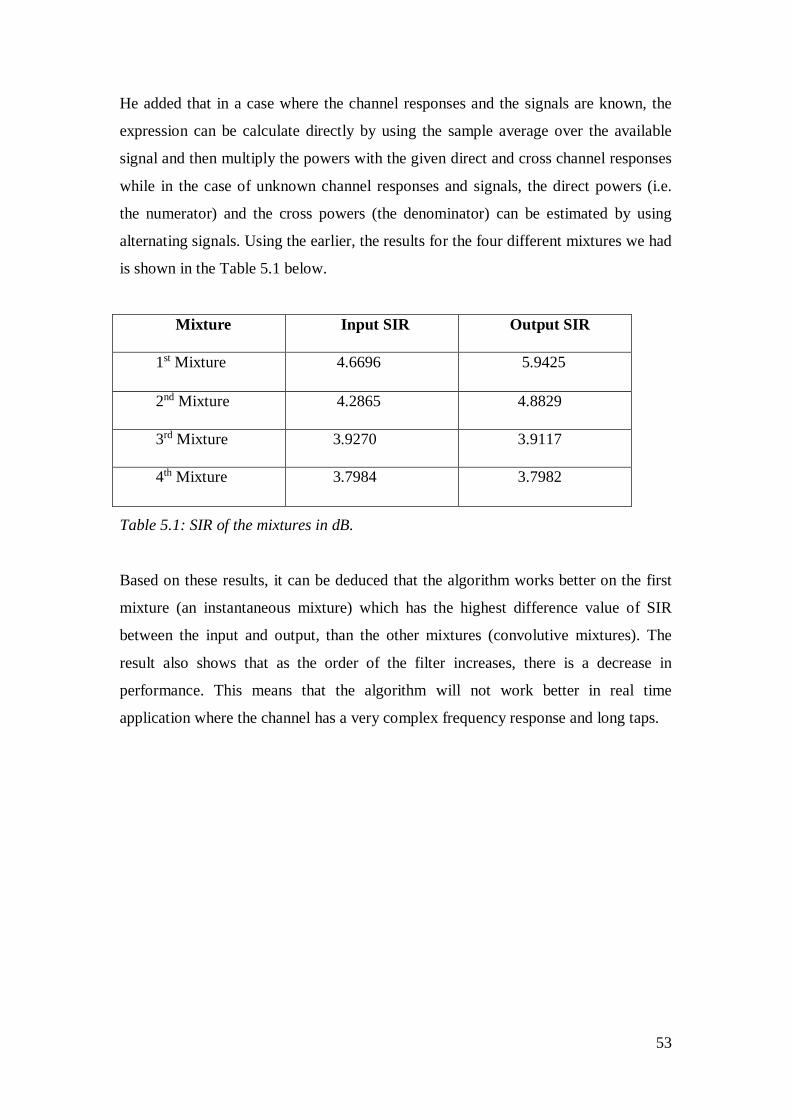
He added that in a case where the channel responses and the signals are known, the

expression can be calculate directly by using the sample average over the available

signal and then multiply the powers with the given direct and cross channel responses

while in the case of unknown channel responses and signals, the direct powers (i.e.

the numerator) and the cross powers (the denominator) can be estimated by using

alternating signals. Using the earlier, the results for the four different mixtures we had

is shown in the Table 5.1 below.

Mixture Input SIR Output SIR

1st Mixture 4.6696 5.9425

2nd Mixture 4.2865 4.8829

3rd Mixture 3.9270 3.9117

4th Mixture 3.7984 3.7982

Table 5.1: SIR of the mixtures in dB.

Based on these results, it can be deduced that the algorithm works better on the first

mixture (an instantaneous mixture) which has the highest difference value of SIR

between the input and output, than the other mixtures (convolutive mixtures). The

result also shows that as the order of the filter increases, there is a decrease in

performance. This means that the algorithm will not work better in real time

application where the channel has a very complex frequency response and long taps.

53

Chapter 6

6.1 Conclusion

In our thesis work, we have studied and implemented the Frequency domain Blind

source separation, using Independent Component Analysis, which can be used in

applications like teleconference, hearing-aids etc. This is a very attractive method in

solving convolutive mixture signals, which is the only form of mixtures applicable in

real time applications. We looked at the formulation of the Independent Component

Analysis algorithm based on higher order statistics which lead us to talk about some

statistical terms. The frequency domain ICA requires that the time domain mixture

signal be transformed into Frequency Domain and this is done with Short Time

Fourier Transform (STFT). This gave us an edge to study the Short Time Fourier

Transform (STFT), its methods, applications and benefits.

Of course the study of Frequency Domain BBS/ICA didn’t just go without difficulties

and problems, the most prominent one is the familiar problem with Frequency domain

BSS/ICA and that is the permutation and Scaling alignment problem which is our

main target in this work to resolve. We looked at different methods some researchers

have used to mitigate the problem, and applied one of them in our approach.

Our result shows that the method proposed by Minje et al in [12] for permutation

resolution works well on “offline” or artificial mixture. The scaling resolution method

proposed by Makino et al also works well.

We will finally recommend that more work should be done in the permutation

problem (with more regards to speed and simplicity) and to increase the speed of

convergence of the ICA algorithm, methods like the FastICA [5, 7, 9] should be

considered.

54

References

[1] J.Benesty, S.Makino and J.Chen, Speech Enhancement. Springer, 2005.

[2] Monson H. Hayes, Statistical Digital Signal Processing and Modeling. New

York: Wiley Corporation, 1996.

[3] Ivan Selesnick, Short Time Fourier Transform. Connexions, Aug. 9, 2005.

[4] Nedelko Grbic, Neural Networks, Department of Telecommunications and

Signal Processing, Blekinge Institute of Technology, Sep. 27, 2004

[5] Aapo Hyvärinen, Juha Karhunen and Erikki Oja, Independent Component

Analysis. John Wiley & Sons, Incorporation, 2001.

[6] John G Proakis and Dimitris G Manolakis: Digital Signal Processing. 3rd

edition, Upper Saddle River, N.J.: Prentice-Hall Corporation, 1996.

[7] Aapo Hyvärinen, Fast and Roust Fixed-Point Algorithms for Independent

Component Analysis. IEEE Transactions on Neural Networks, Volume 10,

NO. 3, May 1999.

[8] Aapo Hyvärinen and Erkki Oja, Independent Component Analysis: Algorithms

and Applications. Neural Networks Research Centre, Helsinki University of

Technology, http://www.cis.hut.fi/projects/ica, 2000.

[9] Hiroshi Sawada, Ryo Mukai, Shoko Araki and Shoji Makino, A Robust and

Precise Method for Solving the Permutation Problem of Frequency- Domain

Blind source Separation. IEEE Transactions on Speech and Audio Processing,

Vol. 12, No. 5, September 2004.

[10] http://en.wikipedia.org/wiki/

[11] P. Smaragdis, Blind Separation of Convolved mixtures in the Frequency

Domain. Neurocomputing, No. 22, Pages 21 – 34, 1998.

[12] Minje Kim and Seungjin Choi, ICA-Based Clustering for Resolving

Permutation Ambiguity in Frequency-Domain Convolutive Source Separation.

IEEE, 18th International conference on Pattern Recognition, 2006.

[13] Shun–Ichi Amari, Natural gradient works efficiently in learning, Neural

Computation, No. 10, Pages 251 – 276, 1998.

55

[14] Pando Georgiev, Andrzej Cichocki and Shun-ichi Amari, On some extensions

of the Natural Gradient Algorithm. Proceeds 3rd International Conference. on

Independent Component Analysis (ICA 2001)

[15] Simon Haykin, Neural Networks, A comprehensive Foundation. 2nd edition,

Upper Saddle River, N.J.: Prentice-Hall Corporation, 1999.

[16] P. Comon, Independent Component Analysis, a new concept?. Signal

Processing, Elsevier, 36(3): Pages 287 – 314, April 1994, Special Issue on

Higher-Order Statistics.

[17] http://www.cnl.salk.edu/~tewon/Blind/blind_audio.html

[18] http://www.bth.se/tek/asb.nsf/$DefaultView/FAE6B018478855F9C12571AF0044320D

[19] Nedelko Grbic, Xiao-Jiao Tao, Sven Erik Nordholm, Ingvar Claesson, Blind

Signal Separation Using Overcomplete Subband Representation. IEEE

Transactions on Speech and Audio Processing, Vol. 9, NO. 5, July 2001

[20] Lucas Parra and Clay Spence, Convolutive Blind Separation of Non-Stationary

Sources. IEEE Transactions on Speech and Audio Processing, Vol 8, NO. 3,

May 2000.

56