Blind Image Restoration by using PCA-Subspace

Generation and Image Quality Optimization

Brian Sumali1, Haslina Sarkan2, Nozomu Hamada1

MJIIT1, AIS2

Universiti Teknologi Malaysia

Kuala Lumpur, Malaysia

sbrian2@live.utm.my, (haslinams, hamada)@utm.my

Yasue Mitsukura

Department of System Design Engineering

Faculty of Science and Technology, Keio University

Yokohama, Japan

mitsukura@sd.keio.ac.jp

Abstract—Image blurring process is commonly formulated as

two-dimensional convolution between the latent image and the

blurring system. Blind image restoration problem is to estimate

the latent image only from the blurred image. Conventional blind

image restoration techniques tend to solve this problem by

estimating the blurring system and therefore their effectiveness

are dependent to the accuracy of their estimation. Principal

Component Analysis (PCA)-based restoration technique,

however, do not employ PSF estimation and still gives high

restoration quality. PCA-based techniques have two different

roots. The first is to boost the high-frequency component lost

during the blurring process by maximizing the image variance.

The other comes from source-separation using PCA. Previously

we proposed a PCA-generated subspace for blind restoration and

proved its superiority to conventional methods. However, the

algorithm should be improved. This study proposes a sign-

determination method and modify the image quality optimization

technique. The noise robustness and the application to other blurs

are also investigated in this paper. From the experiments, we can

see that the proposed method gives higher restoration quality both

for simulated blur images and real images than conventional

methods.

Keywords—Blind image restoration; Single image restoration;

Principal Component Analysis; Image enhancement; Image

quality

I. INTRODUCTION

Image restoration is to remove all degradations from a corrupted observation and estimate the original, pristine images. Degradations come in many types such as motion blur, camera defocus, noise, atmospheric turbulence, and many others. Typical image restoration techniques assume blur-induced degradations as a system called point-spread-function (PSF). The corrupted observation is assumed as a result of a convolution between the pristine image with the PSF and addition with noise. Based on these assumptions, typical image restoration techniques estimate the inverse of degradation system and the restoration is performed by convolving the corrupted observation with the inverse system. Therefore, an image restoration is a deconvolution process. Although these assumptions imply that the degradation process is a linear process and shift-invariant, which is not true for real world’s cases, this model is still used because it simplifies the problem. The simplest image restoration algorithm is the inverse filter [1].

In real world cases, there is almost no information available regarding the PSF nor the original image and it is usually defined as an ill-posed problem where there are multiple possible combinations of latent image and PSF. The techniques designed to tackle this ill-posed problem is called blind image restoration or blind image deconvolution technique. Up to now, numerous blind deconvolution algorithms have been developed in many fields, such as medical imaging, astronomy, remote sensing, optics and daily life. An overview of conventional blind image restoration techniques are available from [2]-[5].

Conventional blind image restoration techniques can be categorized into two types: The first kind is by estimating the PSF of the degradation system from given observation and perform deconvolution using the inverse system. The algorithms in this category are usually straight forward and only concerned about PSF estimation. The algorithms on the second category are called joint estimation which simultaneously estimate the PSF and the latent image. These algorithms are usually more complex than the first category.

Lane and Bates proposed zero sheet approach [6] for multi-dimensional deconvolution. Ayers and Dainty [7] applies alternating estimation between the PSF and the original image in the Fourier domain and under the non-negativity constraints during iterations. Another example is the blind implementation of Lucy-Richardson algorithm [8],[9] that estimates both PSF and original image using Lucy-Richardson Algorithm by Fish et al. [10]. While not needing correct estimation of the degrading PSF, this algorithm still imposes prior assumption for PSF.

Gradient magnitude distribution of natural images were incorporated for camera-shake or motion-blur PSF estimation by Fergus et al. [11]. However, their algorithm still impose a user input and not fully-automatic. Recently, this weakness was improved by L. W. Chang and J. T. Chang for automated patch selection [12]. Levin et al. [13], [14] proposed a MAP𝑘 algorithm. They argued that MAP estimation over the blurring system is more accurate compared to conventional MAP𝑥,𝑘

algorithms [11], [15], [16] that often failed to perform restoration.

In contrast with conventional blind restoration algorithms, PCA-based restoration algorithms do not use inverse filtering to recover the image. This approach was pioneered by Li et al. [17]. Blurring process reduces the image’s variance and removes the

high-frequency component. Their idea is to boost the missing high-frequency component by enhancing the variance of the deconvolved image. They designed a deconvolution FIR filter with unity filter norm constraints by maximizing variance of output image of the deconvolution filter. Their succeeding work [18] improves their previously multi-frame algorithm to solve single-channel algorithm by creating ensemble of horizontal and vertically shifted degraded images. Both approaches perform the restoration by adding the first principal component to the degraded image.

Our previous approaches [19]-[22] implemented PCA but with a several differences from [18]. Ensemble generation process by Gaussian smoothing instead of shifting the observed image was proposed in [19]. The restoration quality was also improved by incorporating the second principal components instead of only the first. NIQE [23], a no-reference image quality assessment index (NR-IQA) was introduced in [20] to control the iteration number.

In [21] we proposed to employ magnitude scaling to the principal components and also investigated the optimal parameters for ensemble generation process. We generalized the PCA-based blind image restoration into an optimization problem by maximizing a NR-IQA’s score in [22]

Although this study is also focused on atmospheric turbulence-degraded image and based on PCA for restoring high-frequency components in the same way as our previous studies [21], [22], some investigations and modifications have been done to improve the previous approach. The novel contributions are as follows:

1. We introduced sign determination and modified the optimization algorithm. This improves the restoration quality.

2. The noise robustness of the proposed algorithm is evaluated and improved.

3. We show that our method can be applied for other types of blur, not only Gaussian blur or atmospheric turbulence.

The rest of this paper is structured as follows: In II, a review for our PCA-based image restoration methods is presented. Our proposed modifications are described in III, and some experimental results are shown in IV. The paper is then concluded in V.

II. PCA-BASED IMAGE RESTORATION

A. Basic idea of PCA-based approach

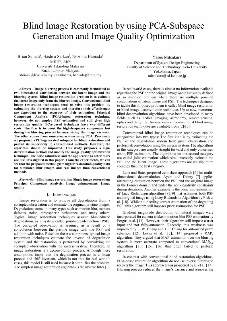
Fig. 1 illustrates a basic idea behind our PCA approach. The

original image and the blurred image are represented by two

vectors 𝑓, 𝑔(= 𝑔1) in image vector space respectively.

Another set of image vectors 𝑔2, 𝑔3, ⋯ , 𝑔𝑀 are generated by

further blurs with known PSF where 𝑔𝑖+1 is blurred from 𝑔𝑖

recursively up to 𝑖 = 𝑀 − 1. By utilizing the image vector

which is derived from subtracting image 𝑔2 from 𝑔1, we may

generate a 1-D subspace or linear space with scalar parameter

λ as; 𝑔1 + 𝜆(𝑔1 − 𝑔2) (1)

Since 𝑔2 is the blurred image from 𝑔1 , the subtraction part

λ(𝑔1 − 𝑔2) with appropriate λ would be considered as an

approximated high frequency component image which was lost

by the further blurring process. Conventional unsharp masking

[24] uses a similar idea which was developed for image

enhancing such as edge or contrast enhancement. However in

the PCA-based technique we generate multiple blurred images

and apply PCA for generating higher orthogonal subspace. If

we generate M blurred image and utilize the resulting major J

orthogonal principal components as shown in Fig. 1, restoration

process will be performed in J-dimensional subspace. A

detailed mathematical development about the proposed

approach will be discussed the proceeding sections.

B. PCA-subspace image restoration

Before applying the restoration method, the blurred image 𝑔 needs to be preprocessed into column vector 𝒈. The restoration method we proposed consisted of several steps:

1. Generate an ensemble of M blurred images.

𝒈1 = 𝒈 (2)

𝒈𝑖 = 𝒈𝑖−1 ∗ 𝑏(σ); 𝑖 = 2~M

where 𝒈 is the blurred image and 𝑏(σ) is the Gaussian smoothing PSF with standard deviaton of σ.

2. Compute the average image 𝜳 from the ensemble.

𝜳 =1

𝑀∑ 𝒈𝑖

𝑀

𝑖=1

(3)

3. Center the ensemble by removing the mean.

𝝓𝑖 = 𝒈𝑖 − 𝜳 (4)

𝑨 = [𝝓1, 𝝓2, … , 𝝓𝑀]

4. Extract the principal components

The principal components from the ensemble is the eigenvector of covariance matrix:

𝑪𝜙 =1

𝑀𝑨𝑨𝑇 (5)

Fig. 1 Basic idea of PCA-based image restoration

where the size of 𝑪𝜙 is (𝑅 ∙ 𝐶) × (𝑅 ∙ 𝐶) in case of 𝑅 × 𝐶 being

the size of 𝒈 . Computing 𝑪𝜙 itself needs extremely large

resource. To reduce the computational burden, Turk et al. [ref from nakamura] proposed to compute the eigen-decomposition of 𝑨𝑇𝑨 first.

𝑪𝜙𝑇 = 𝑨𝑇𝑨

(6) 𝑪𝜙

𝑇 𝒖 = λ 𝒖

Then, w pre-multiply both sides with 𝑨, to get the principal components of 𝑪𝜙.

𝑨𝑪𝜙𝑇 𝒖 = λ 𝑨𝒖

(7) 𝑨𝑨𝑇𝑨𝒖 = λ 𝑨𝒖

𝑪𝜙𝑨𝒖 = λ 𝑨𝒖

𝒗 = 𝑨𝒖

where 𝒗 is the principal components of 𝑪𝜙

5. Estimate the pristine image

We define the restored image as a linear combination of scaled principal components.

�̂� = 𝒇�̂� = 𝜳 + ∑ 𝛼𝑖

𝑱

𝒊=𝟏

𝒗𝒊; 𝐽 < 𝑀, 𝐽 ∈ ℕ (8)

where 𝒗𝒊 is the i-th principal components and 𝛼𝑖 is the “weight”, a scalar to control the magnitude of 𝒗𝒊 . The set of optimal weights 𝛼𝑖(𝑖 = 1~𝐽) are successively determined by

maximizing the adopted NR-IQA value of the estimate 𝒇�̂�. As

an illustration, the most ideal restored image �̂� will be the projection of latent image 𝒇 to the subspace spanned by principal components 𝒗𝟏~𝒗𝑱 .

Optimal 𝛼1:

𝛼1̂ = arg max 𝑁𝑅𝐼𝑄𝐴(𝒇1̂) (9)

where

𝒇0̂ = 𝜳 (10)

𝒇�̂� = 𝒇𝑖−1̂ + 𝛼1̂𝒗𝒊 (11)

Optimal 𝛼𝑖(𝑖 ≥ 2) can be found by using

𝛼�̂� = arg max 𝑁𝑅𝐼𝑄𝐴(𝒇�̂�) (12)

C. Image Quality Assessment

Image quality assessment (IQA) is a technique to objectively evaluate an image’s quality. When an IQA algorithm predicts an image’s quality by comparing it with reference image, it is called Full-Reference IQA (FR-IQA). Examples of FR-IQA algorithms include MSE, PSNR, SSIM [25], FSIM [26], and GMSD [27]. The FR-IQA algorithms are useful for evaluating the effectiveness of an image restoration algorithm.

There is also a branch of IQA technique that evaluates an image’s quality without any need of reference image: No-Reference IQA (NR-IQA). NR-IQA techniques usually compare the test image with their training database: a pair of image

database and human subjective opinion score. However, recent development of NR-IQA bring forth a “completely blind” indexes that do not utilize human subjective opinion. In this paper, NR-IQA is utilized for determining optimal weight for restoration. NR-IQA and optimization technique chosen to optimize the weights highly affect the restoration quality of PCA-based method. Some example of NR-IQAs are BRISQUE [28], NIQE [23], IL-NIQE [29], and GM-LOG [30].

III. PROPOSED METHOD

A. Contribution ratio of principal components

Previously, we blindly use all the principal components by setting 𝐽 = 𝑀 − 1. Now, we conducted a small experiment to investigate the number of principal components contributing for restoration. The experiment was conducted using ten images that were degraded using Gaussian blur with varying strength, 0 =1, 1.25, 1.5, 1.75, 2.Then, those images were restored using the cost function in Eq .(8) with a slight modification. PSNR, a FR-IQA is used to optimize the weights in place of NR-IQA. The parameters for ensemble generation were 𝑀 = 14, = 0.3, 𝐽 =13.

In Fig. 2, the results of this small experiment are described. These results were from the average of all 10 images. The Y axis shows the contribution in terms of PSNR. The results on Fig. 2 show that in most cases only the first four principal components contribute to restoration process. In most cases, there is nearly no contribution from 5th and further principal components.

B. Sign determination and optimization algorithm

In a rare case, our previous algorithm fail to perform a restoration and instead further degrades the input image. This is caused by the combination of hill-climbing algorithm as an optimization method and the NR-IQA to optimize the restoration quality. Generally, plotting an NR-IQA index versus weight of principal component generates an oscillating plot. Occasionally, the starting point is the oscillating point, causing the hill-climbing to choose the wrong direction for the weight. To tackle this problem, we propose to use the dot product to determine the correct sign (direction of principal components) such that they do not degrade the image. The steps for determining the correct sign are:

1. Compute ∆𝑔 by

∆𝑔 = 𝑔 − (13)

2. Compute the dot product of each principal components.

𝑑𝑖 = ∆𝑔 ∙ 𝑣𝑖 ; 𝑖 = 1~𝐽 (14)

3. Determine the sign for each principal components

𝑠𝑖 = {1 𝑑𝑖 > 0

−1 otherwise

(15)

By applying this sign determination algorithm, the optimization technique need only to check in either positive or negative region. Because a standard hill-climbing algorithm cannot be “forced” to check into only a certain direction, a modification to the hill-climbing algorithm was needed.

We proposed to add an exhaustive search before applying hill-climbing search. The flowchart of our modified hill-

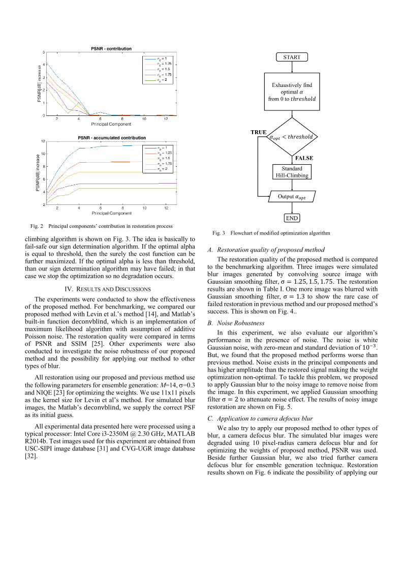
climbing algorithm is shown on Fig. 3. The idea is basically to fail-safe our sign determination algorithm. If the optimal alpha is equal to threshold, then the surely the cost function can be further maximized. If the optimal alpha is less than threshold, than our sign determination algorithm may have failed; in that case we stop the optimization so no degradation occurs.

IV. RESULTS AND DISCUSSIONS

The experiments were conducted to show the effectiveness of the proposed method. For benchmarking, we compared our proposed method with Levin et al.’s method [14], and Matlab’s built-in function deconvblind, which is an implementation of maximum likelihood algorithm with assumption of additive Poisson noise. The restoration quality were compared in terms of PSNR and SSIM [25]. Other experiments were also conducted to investigate the noise robustness of our proposed method and the possibility for applying our method to other types of blur.

All restoration using our proposed and previous method use

the following parameters for ensemble generation: M=14, =0.3 and NIQE [23] for optimizing the weights. We use 11x11 pixels as the kernel size for Levin et al’s method. For simulated blur images, the Matlab’s deconvblind, we supply the correct PSF as its initial guess.

All experimental data presented here were processed using a typical processor: Intel Core i3-2350M @ 2.30 GHz, MATLAB R2014b. Test images used for this experiment are obtained from USC-SIPI image database [31] and CVG-UGR image database [32].

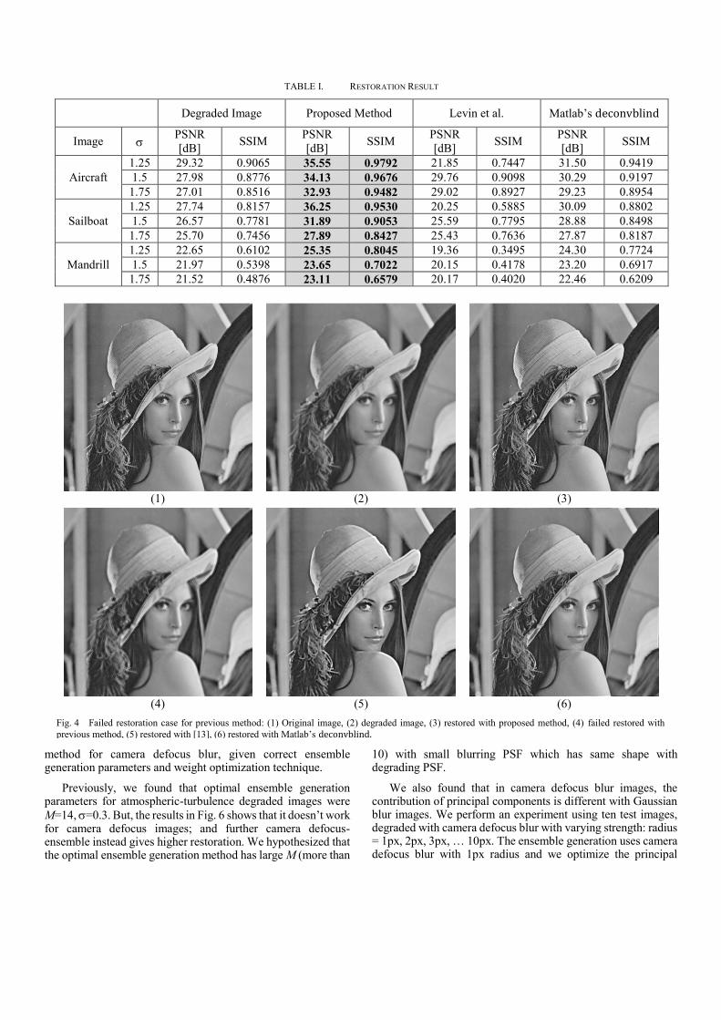
A. Restoration quality of proposed method

The restoration quality of the proposed method is compared to the benchmarking algorithm. Three images were simulated blur images generated by convolving source image with Gaussian smoothing filter, σ = 1.25, 1.5, 1.75. The restoration results are shown in Table I. One more image was blurred with Gaussian smoothing filter, σ = 1.3 to show the rare case of failed restoration in previous method and our proposed method’s success. This is shown on Fig. 4..

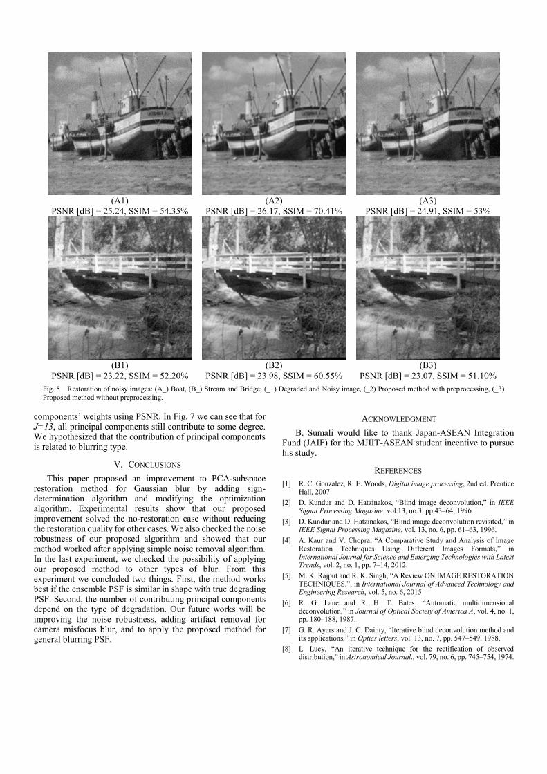
B. Noise Robustness

In this experiment, we also evaluate our algorithm’s performance in the presence of noise. The noise is white Gaussian noise, with zero-mean and standard deviation of 10−3. But, we found that the proposed method performs worse than previous method. Noise exists in the principal components and has higher amplitude than the restored signal making the weight optimization non-optimal. To tackle this problem, we proposed to apply Gaussian blur to the noisy image to remove noise from the image. In this experiment, we applied Gaussian smoothing filter σ = 2 to attenuate noise effect. The results of noisy image restoration are shown on Fig. 5.

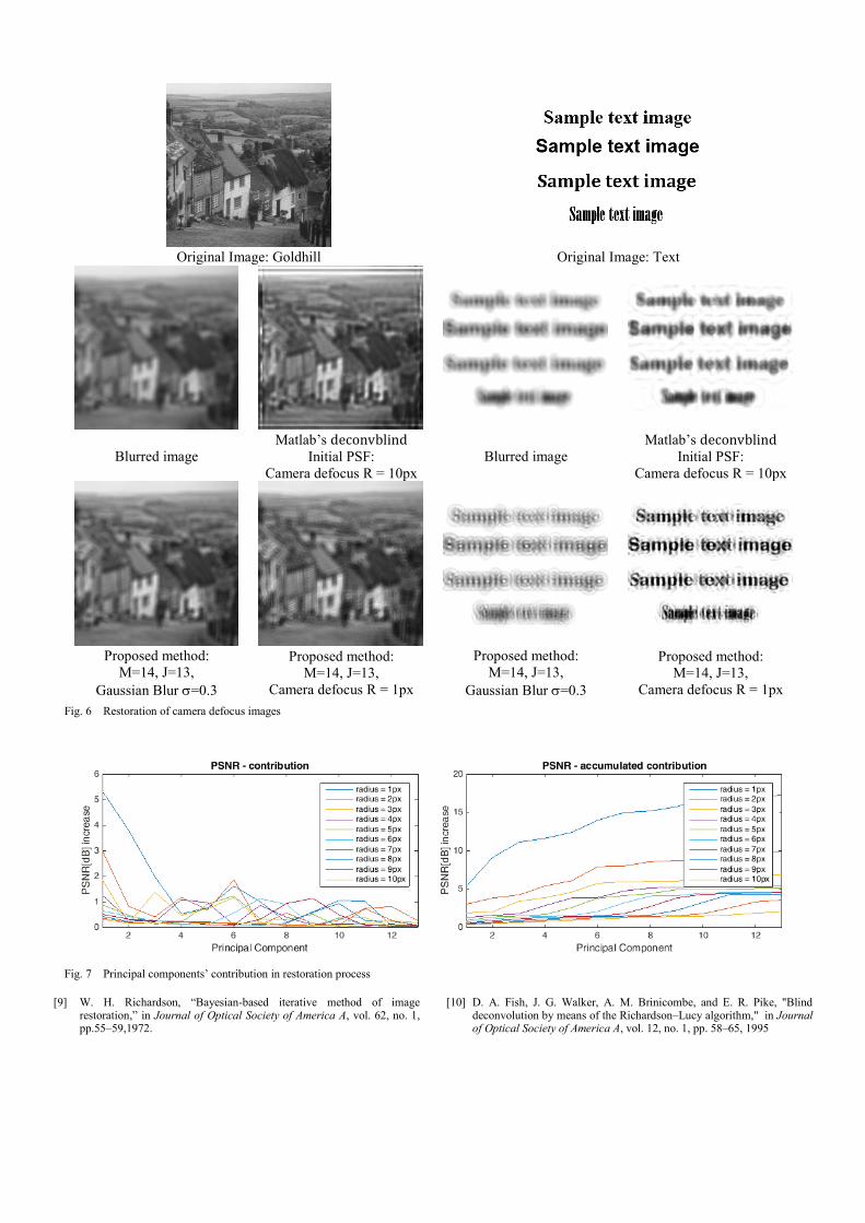
C. Application to camera defocus blur

We also try to apply our proposed method to other types of blur, a camera defocus blur. The simulated blur images were degraded using 10 pixel-radius camera defocus blur and for optimizing the weights of proposed method, PSNR was used. Beside further Gaussian blur, we also tried further camera defocus blur for ensemble generation technique. Restoration results shown on Fig. 6 indicate the possibility of applying our

Fig. 2 Principal components’ contribution in restoration process

Fig. 3 Flowchart of modified optimization algorithm

method for camera defocus blur, given correct ensemble generation parameters and weight optimization technique.

Previously, we found that optimal ensemble generation parameters for atmospheric-turbulence degraded images were

M=14, =0.3. But, the results in Fig. 6 shows that it doesn’t work for camera defocus images; and further camera defocus-ensemble instead gives higher restoration. We hypothesized that the optimal ensemble generation method has large M (more than

10) with small blurring PSF which has same shape with degrading PSF.

We also found that in camera defocus blur images, the contribution of principal components is different with Gaussian blur images. We perform an experiment using ten test images, degraded with camera defocus blur with varying strength: radius = 1px, 2px, 3px, … 10px. The ensemble generation uses camera defocus blur with 1px radius and we optimize the principal

(1) (2) (3)

(4) (5) (6)

Fig. 4 Failed restoration case for previous method: (1) Original image, (2) degraded image, (3) restored with proposed method, (4) failed restored with

previous method, (5) restored with [13], (6) restored with Matlab’s deconvblind.

TABLE I. RESTORATION RESULT

Degraded Image Proposed Method Levin et al. Matlab’s deconvblind

Image PSNR

[dB] SSIM

PSNR

[dB] SSIM

PSNR

[dB] SSIM

PSNR

[dB] SSIM

Aircraft

1.25 29.32 0.9065 35.55 0.9792 21.85 0.7447 31.50 0.9419

1.5 27.98 0.8776 34.13 0.9676 29.76 0.9098 30.29 0.9197

1.75 27.01 0.8516 32.93 0.9482 29.02 0.8927 29.23 0.8954

Sailboat

1.25 27.74 0.8157 36.25 0.9530 20.25 0.5885 30.09 0.8802

1.5 26.57 0.7781 31.89 0.9053 25.59 0.7795 28.88 0.8498

1.75 25.70 0.7456 27.89 0.8427 25.43 0.7636 27.87 0.8187

Mandrill

1.25 22.65 0.6102 25.35 0.8045 19.36 0.3495 24.30 0.7724

1.5 21.97 0.5398 23.65 0.7022 20.15 0.4178 23.20 0.6917

1.75 21.52 0.4876 23.11 0.6579 20.17 0.4020 22.46 0.6209

components’ weights using PSNR. In Fig. 7 we can see that for J=13, all principal components still contribute to some degree. We hypothesized that the contribution of principal components is related to blurring type.

V. CONCLUSIONS

This paper proposed an improvement to PCA-subspace restoration method for Gaussian blur by adding sign-determination algorithm and modifying the optimization algorithm. Experimental results show that our proposed improvement solved the no-restoration case without reducing the restoration quality for other cases. We also checked the noise robustness of our proposed algorithm and showed that our method worked after applying simple noise removal algorithm. In the last experiment, we checked the possibility of applying our proposed method to other types of blur. From this experiment we concluded two things. First, the method works best if the ensemble PSF is similar in shape with true degrading PSF. Second, the number of contributing principal components depend on the type of degradation. Our future works will be improving the noise robustness, adding artifact removal for camera misfocus blur, and to apply the proposed method for general blurring PSF.

ACKNOWLEDGMENT

B. Sumali would like to thank Japan-ASEAN Integration Fund (JAIF) for the MJIIT-ASEAN student incentive to pursue his study.

REFERENCES

[1] R. C. Gonzalez, R. E. Woods, Digital image processing, 2nd ed. Prentice Hall, 2007

[2] D. Kundur and D. Hatzinakos, “Blind image deconvolution,” in IEEE Signal Processing Magazine, vol.13, no.3, pp.43–64, 1996

[3] D. Kundur and D. Hatzinakos, “Blind image deconvolution revisited,” in IEEE Signal Processing Magazine, vol. 13, no. 6, pp. 61–63, 1996.

[4] A. Kaur and V. Chopra, “A Comparative Study and Analysis of Image Restoration Techniques Using Different Images Formats,” in International Journal for Science and Emerging Technologies with Latest Trends, vol. 2, no. 1, pp. 7–14, 2012.

[5] M. K. Rajput and R. K. Singh, “A Review ON IMAGE RESTORATION TECHNIQUES.”, in International Journal of Advanced Technology and Engineering Research, vol. 5, no. 6, 2015

[6] R. G. Lane and R. H. T. Bates, “Automatic multidimensional deconvolution,” in Journal of Optical Society of America A, vol. 4, no. 1, pp. 180–188, 1987.

[7] G. R. Ayers and J. C. Dainty, “Iterative blind deconvolution method and its applications,” in Optics letters, vol. 13, no. 7, pp. 547–549, 1988.

[8] L. Lucy, “An iterative technique for the rectification of observed distribution,” in Astronomical Journal., vol. 79, no. 6, pp. 745–754, 1974.

(A1)

PSNR [dB] = 25.24, SSIM = 54.35%

(A2)

PSNR [dB] = 26.17, SSIM = 70.41%

(A3)

PSNR [dB] = 24.91, SSIM = 53%

(B1)

PSNR [dB] = 23.22, SSIM = 52.20%

(B2)

PSNR [dB] = 23.98, SSIM = 60.55%

(B3)

PSNR [dB] = 23.07, SSIM = 51.10%

Fig. 5 Restoration of noisy images: (A_) Boat, (B_) Stream and Bridge; (_1) Degraded and Noisy image, (_2) Proposed method with preprocessing, (_3)

Proposed method without preprocessing.

[9] W. H. Richardson, “Bayesian-based iterative method of image restoration,” in Journal of Optical Society of America A, vol. 62, no. 1, pp.55–59,1972.

[10] D. A. Fish, J. G. Walker, A. M. Brinicombe, and E. R. Pike, "Blind deconvolution by means of the Richardson–Lucy algorithm," in Journal of Optical Society of America A, vol. 12, no. 1, pp. 58–65, 1995

Original Image: Goldhill Original Image: Text

Blurred image

Matlab’s deconvblind

Initial PSF:

Camera defocus R = 10px

Blurred image

Matlab’s deconvblind

Initial PSF:

Camera defocus R = 10px

Proposed method:

M=14, J=13,

Gaussian Blur =0.3

Proposed method:

M=14, J=13,

Camera defocus R = 1px

Proposed method:

M=14, J=13,

Gaussian Blur =0.3

Proposed method:

M=14, J=13,

Camera defocus R = 1px

Fig. 6 Restoration of camera defocus images

Fig. 7 Principal components’ contribution in restoration process

[11] R. Fergus, B. Singh, A. Hertzmann, S.T. Roweis, and W.T. Freeman, “Removing camera shake from a single photograph,” in The 33rd International Conference and Exhibition on Computer Graphics and Interactive Techniques (SIGGRAPH), 2006.

[12] Ju-Ting Chang and Long-Wen Chang, “Image Decomposition and Patch Selection for Single Image Blind Deblurring”, in The Eighth International Workshop on Image Media Quality and its Applications (IMQA), Nagoya (Japan), 2016

[13] A. Levin, Y. Weiss, F. Durand, and W. T. Freeman, “Understanding and evaluating blind deconvolution algorithms,” in IEEE Conference on Computer Vision and Pattern Recognition (CVPR), pp. 1964–1971., 2009

[14] A. Levin, Y. Weiss, F. Durand, and W. T. Freeman, “Efficient marginal likelihood optimization in blind deconvolution,” in IEEE Conference on Computer Vision and Pattern Recognition (CVPR), pp.2657–2664, 2011

[15] A. Levin, “Blind motion deblurring using image statistics,” in Advances in Neural Information Processing Systems (NIPS), 2006.

[16] J. W. Miskin and D. J. C. MacKay, “Ensemble learning for blind image separation and deconvolution,” in Advances in Independent Component Analysis, Springer, 2000.

[17] Dalong Li, S. Simske, and R. M. Mersereau, “Blind image deconvolution using constrained variance maximization,” in The Thirty-Eighth Asilomar Conference on Signals, Systems and Computers, vol.2, pp.1762–1765 Vol.2, 2004

[18] Dalong Li, R. M. Mersereau, and S. Simske, “Atmospheric Turbulence-Degraded Image Restoration Using Principal Components Analysis,” in IEEE Geoscience and Remote Sensing Letters, vol.4, no.3, pp.340–344, 2007

[19] R. Nakamura, Y. Mitsukura, and N. Hamada, “Iterative PCA approach for blind restoration of single blurred image,” in International Symposium on Intelligent Signal Processing and Communications Systems (ISPACS), pp.543–546, 2013

[20] R. Nakamura, Y. Mitsukura, and N. Hamada, “Blind restoration of single-channel image using iterative PCA,” in IEEE Conference on Systems, Process & Control (ICSPC), pp.84–87, 2013

[21] B. Sumali, N. Hamada, and Y. Mitsukura, “Blind Image Restoration Method by PCA-based Subspace Generation”, in International

Symposium on Intelligent Signal Processing and Communication Systems (ISPACS), pp. 204-209, Bali, Indonesia, 2015

[22] B. Sumali, N. Hamada, and Y. Mitsukura, “Blind Image Restoration using PCA and Image Quality Assessment”, in The Eighth International Workshop on Image Media Quality and its Applications (IMQA), Nagoya, Japan, 2016

[23] A. Mittal, R. Soundararajan, and A. C. Bovik, “Making a 'Completely Blind' Image Quality Analyzer,” in IEEE Signal Processing Letters, vol.20, no.3, pp.209–212, 2013

[24] A. Jain, “Image Enhancement,” in Fundamentals of Digital Image Processing, Prentice-Hall, 1989

[25] Zhou Wang, A. C. Bovik, H. R. Sheikh, and E. P. Simoncelli, “Image quality assessment: from error visibility to structural similarity,” in IEEE Transactions on Image Processing, vol.13, no.4, pp.600–612, 2004

[26] Lin Zhang, Lei Zhang, Xuanqin Mou, and David Zhang, “FSIM: a feature similarity index for image quality assessment”, in IEEE Transactions on Image Processing, vol. 20, no. 8, pp. 2378–2386, 2011

[27] W. Xue, L. Zhang, X. Mou, and A. C. Bovik, “Gradient magnitude similarity deviation: a highly efficient perceptual image quality index,” in IEEE Transactions on Image Processing, vol. 23, no. 2, pp. 684–695, 2014.

[28] A. Mittal, A. K. Moorthy and A. C. Bovik, “ No-Reference Image Quality Assessment in the Spatial Domain “, in IEEE Transactions on Image Processing, 2012

[29] Lin Zhang, Lei Zhang, and A. C. Bovik, “A Feature-Enriched Completely Blind Image Quality Evaluator,” in IEEE Transactions on Image Processing, vol.24, no.8, pp.2579–2591, 2015

[30] W. Xue, X. Mou, L. Zhang, A. C. Bovik, and X. Feng, “Blind image quality assessment using joint statistics of gradient magnitude and laplacian features,” in IEEE Transactions on Image Processing, vol. 23, no. 11, pp. 4850–4862, 2014.

[31] University of Southern California. USC-SIPI Image Database [Online]. Available: http://sipi.usc.edu/database/

[32] University of Granada. CVG–UGR Image Database Computer Vision Group [Online]. Available: http://decsai.ugr.es/cvg/dbimagenes/