Bivariate splines for ozone concentration forecastingmath.uga.edu/~mjlai/papers/EGL12.pdf · Research Article Environmetrics Received: 20 June 2011, Revised: 22 March 2012, Accepted:

Research Article Environmetrics

Received: 20 June 2011, Revised: 22 March 2012, Accepted: 5 April 2012, Published online in Wiley Online Library: 11 May 2012

(wileyonlinelibrary.com) DOI: 10.1002/env.2147

Bivariate splines for ozone concentrationforecastingBree Ettingera*, Serge Guillasb and Ming-Jun Laic

In this paper, we forecast ground level ozone concentrations over the USA, using past spatially distributed measurementsand the functional linear regression model. We employ bivariate splines defined over triangulations of the relevant regionof the USA to implement this functional data approach in which random surfaces represent ozone concentrations. Wecompare the least squares method with penalty to the principal components regression approach. Moderate sample sizesprovide good quality forecasts in both cases with little computational effort. We also illustrate the variability of forecastsowing to the choice of smoothing penalty. Finally, we compare our predictions with the ones obtained using thin-platesplines. Predictions based on bivariate splines require less computational time than the ones based on thin-plate splinesand are more accurate. We also quantify the variability in the predictions arising from the variability in the sample usingthe jackknife, and report that predictions based on bivariate splines are more robust than the ones based on thin-platesplines. Copyright © 2012 John Wiley & Sons, Ltd.

Keywords: functional data; ozone; bivariate splines

1. INTRODUCTIONGround-level ozone is a harmful pollutant (Bell et al., 2004). To inform the public on a daily basis about ozone and other pollutants, theUS Environmental Protection Agency (EPA) has created a simplified index of air quality, the pollutant standards index (PSI), and sinceJuly 1999, EPA replaced the PSI with the Air Quality Index. Forecasts of these indices made 24 h ahead have been provided to newspapersin various regions so that people can avoid outdoor activities likely to damage their health. Using the PSI, Neidell (2010) showed thatair quality warnings associated with ground-level ozone have had an impact on outdoor activities in Southern California, especially forsusceptible local residents. Hence, improving the quality of these forecasts may contribute to better public health.

We consider here ozone concentrations from the network of EPA stations across the USA, over a span of 3 months in the summer of2005. Our goal is to predict the ozone concentration values at a specific location in suburban Atlanta 24 h ahead based on the previous ozoneconcentrations values up to the current hour. There are many available methods, ranging from chemistry-transport models to statistical tech-niques. Recently, Guillas and Lai (2010) initiated a brand new statistical approach to predict ozone concentration values using functionallinear regression with bivariate splines (piecewise polynomial functions over a triangulation of a polygonal domain). The goal is to capturepredictive power in time from spatial synoptic scales, as chemistry and transport occur at regional scales. Such spatio–temporal informationhas been used before to model time-dependent dynamics in hourly ozone concentration fields, for example, Dou et al. (2010). However,our approach represents the surface as a random function, which enables us to carry out regression and prediction in that setting. Modelingobservations as functional data presents many advantages, see Ramsay and Silverman (2005) and Ferraty and Vieu (2006) for an overviewof functional data analysis. For that purpose, one needs a parametric representation of the surfaces ideally in a flexible basis that Kriging isnot able to offer. Guillas and Lai (2010) established the theoretical foundations, even under time-dependence assumptions, of this method forwhich a least squares criterion with penalty is minimized. In the following, we refer to this approach as the “brute force method” (BF). Com-parison with time series approaches using functional data analysis (i.e., in one dimension: time) shows that BF can predict better, particularlywith small sample sizes by borrowing strength across space around the location of interest, see Guillas and Lai (2010) for examples.

Crambes et al. (2009) minimized a residual sum of squares subject to a smoothness penalty as in BF, but modified the usual penalty termof univariate smoothing splines to study the prediction. They showed that the rates of convergence of the estimates of the slope are optimal.Yuan and Cai (2010) demonstrated that BF can deliver optimal rates of convergence for either prediction or estimation. Their setting unifiesthe treatment of estimation and prediction under the umbrella of one family of norms. They showed the interesting property that the fasterthe decay in the eigenvalues of the covariance operator of the explanatory variable, the faster the prediction and the slower the estimationof the slope.

* Correspondence to: Bree Ettinger, MOX - Dipartimento di Matematica, Politecnico di Milano, Milano, Italy. E-mail: [email protected]

a MOX - Dipartimento di Matematica, Politecnico di Milano, Milano, Italy

b Department of Statistical Science, University College London, London, U.K.

c Department of Mathematics, University of Georgia, Athens, GA 30602, U.S.A.

Environmetrics 2012; 23: 317–328 Copyright © 2012 John Wiley & Sons, Ltd.

317

Environmetrics B. ETTINGER, S. GUILLAS AND M.-J. LAI

The Functional Principal Component Regression (FPCR) has been introduced in two papers (Cardot et al., 1999, 2003), which cover thecase of random functional data that are curves. It relies on the principal component decompositions prior to inference about the regressionslope. Cardot et al. (2003) used univariate splines to approximate the empirical estimator for the regressor function associated with therandom functional. FPCR was shown to attain optimal rates of convergence for prediction and estimation (Cai and Hall, 2006; Hall andHorowitz, 2007). As pointed out by Cressie and Wikle (2011), the empirical orthogonal functions (EOFs) employed in space–time analysisof geophysical data are merely principal components for the vector of observations. In practice, EOFs are used since observations are col-lected at discrete points. However, this approach can yield misleading results as these observations are not weighted spatially. The analysisshould reflect the continuous variations of the field. The Karhunen-Loève expansion considered later is the continuous equivalent of the EOFdecomposition. Using bivariate splines, we respect the continuous nature of ozone fields.

In our context of ozone forecasting, Aneiros-Perez et al. (2004) considered a functional additive model and Crambes et al. (2009) appliedleast squares with penalty to the prediction of the maximum of the ground-level ozone concentration. However, these studies do not exploitspatial information. When dealing with random surfaces and a functional associated with these over a domain of irregular shape, bivariatesplines can be an excellent approximation tool, especially when the random surfaces are observed only over scattered locations (Lai, 2008)as these splines possess optimal approximation properties (Lai and Schumaker, 2007). Thus, we shall use these splines in FPCR and wouldlike to know how it compares with BF for the ozone concentration forecasting problem. We shall explain this generalization in the followingsection in detail and discuss the similarities and differences between BF and FPCR in this context. We illustrate numerically the advantagesand disadvantages of these two approaches. The biggest difference lies in the fact that BF is straightforward and can be used for predictionwithout a spectral decomposition whereas the FPCR requires the use of a selected number of eigenvalues and eigenvectors in advance to beeffective for prediction.

Thin-plate splines have been used in various applications to model surfaces, see Wood (2003) and references therein. For instance,Paciorek et al. (2009) considered the measurement of particulate matters concentrations, and used thin-plate splines to represent spatialvariations in a spatio–temporal model. We wish to compare the skills of thin-plate splines and bivariate splines in our problem of spatialrepresentation and prediction of ozone concentrations. For that aim, we compare, in this paper, BF using either thin-plate splines or bivariatesplines. This is the first time that such comparison is carried out.

The paper is organized as follows. We first explain two approaches of prediction with an emphasis on the FPCR in the next section, and weexplain the similarities and differences of these two methods in practice. Then, we present numerical experiments in Section 3. In Section 4,we compare the use of thin-plate splines and bivariate splines. In Section 6, we address the issue of the choice of triangulation. Finally inSection 7, we conclude and discuss some future research directions.

2. TWO APPROACHES OF FORECASTINGLet Y be a real-valued random variable, which is a functional of random surface X . That is, let D be a polygonal domain in R2.The functional linear model for Y is as follows:

Y D f .X/C "D hg;Xi C "D

ZDg.s/X.s/dsC "; (1)

where X is a random surface over D, g.s/ is in a function space H (usually L2.D/), " is a real random variable that satisfies E" D 0 andEX.s/"D 0;8s 2D.

2.1. Brute-force

The BF method is explained in detail in Guillas and Lai (2010). For convenience, let us outline the approach as follows. The estimate of thefunction g 2H is chosen to solve the following minimization problem:

minˇ2H

Eh.Y � hˇ;Xi/2

iC �kˇk22; (2)

where � > 0 is a penalty, and kˇk22 denotes the semi-norm of ˇ:

kˇk22 D

ZD

XiCjD2

�Di1D

j2ˇ�2; (3)

in which Dk denotes the differentiation operator with respect to the kth variable. Our objective is to determine or approximate g which isdefined on a spatial domain D based on observations of X , from a set of design points in D, and of the random variable Y . We choose aspline space Sr

d.4/, that is, the space of polynomials of degree d and smoothness r over the triangulation 4 (Lai and Schumaker, 2007),

which is a finite dimensional subspace of L2.D/.In practice, the random surfaces Xi ’s are not observed continuously, but at design points sk 2 D; k D 1; � � � ; N . The smooth bivariate

spline approximation SXi of Xi is the solution in Srd.4/ of the following minimization

min

8<:NXkD1

jh.sk/�Xi .sk/j2C �En.h/; h 2 Srd .4/

9=; ; (4)

318

wileyonlinelibrary.com/journal/environmetrics Copyright © 2012 John Wiley & Sons, Ltd. Environmetrics 2012; 23: 317–328

BIVARIATE SPLINES Environmetrics

where En.h/DRD�D21h

�2C2.D1D2h/

2C�D22h

�2is a energy functional and � > 0 a smoothing parameter. The existence, uniqueness and

computational scheme can be found in Awanou et al. (2006). The approximation properties of the penalized least squares fit are summarizedin Lai (2008).

We seek an approximation eSg;n 2 Srd .4/ of the empirical estimator of g such that eSg;n minimizes the following:

minˇ2Sr

d.4/

1

n

nXiD1

�Yi � hˇ; SXi i

�2C �kˇk22 (5)

where SXi 2 Srd.4/ is a penalized least squares fit of the ozone data Xi on the hour i using the bivariate spline space Sr

d.4/. The space

of bivariate splines over the domain D, Srd.4/, can be chosen for instance to be S01 .4/ (linear finite elements), S05 .4/ for continuity only,

but with polynomials of degree 5, or S15 .4/ (our actual choice in this paper) for more smoothness across the domain. We choose d D 5 andr D 1 because these values satisfy the minimal requirements for a smooth spline to have the optimal approximation order with d greater than3r C 1, see Th 2.1 in Guillas and Lai (2010). We do not consider here higher degrees because the additional number of degrees of freedomwould require more data to yield some benefit.

Although spline functions are only C 1 differentiable in the case of S15 .4/ over the domain, they are in the Sobolev space H2.4/, andhence, we can use the previously mentioned penalty function with second-order derivatives. Indeed, we compute all second-order derivativesof spline functions inside each triangle (polynomials within each triangle) but not over edges nor at vertices. All edges and vertices of atriangulation form a set of measure zero for the integration in (3).

We use here the representation of splines by their coefficients in the Bernstein–Bezier basis of bivariate polynomials �i ; i D 1; � � � ; m ,for which computations are efficient and continuity and smoothness conditions can easily be derived (Lai and Schumaker, 2007, Chapter 2).

The solution of the above minimization is in Srd.4/ and is given by eSg;n D

PmiD1ecn;i�i with coefficient vector ecn D �ecn;i ; i D 1; � � � ; m�

satisfying fAnecn D ebn, where

fAn D24 1n

nX`D1

h�i ; SXìh�j ; SXì C �E2��i ; �j

�35i;jD1;�� ;m

;

where E2.˛; ˇ/DRDPiCjD2D

i1D

j2˛D

i1D

j2ˇ, corresponds to the semi-norm kˇk22 above, and

ebn D24 1n

nX`D1

Y`h�j ; SXì

35jD1;�� ;m

:

In theory, the spline space Srd.4/ is dense in H as the size j4j of triangulation4 decreases to zero, and hence, the approximation Sg of

the empirical estimator of g in (5) approximates g as the sample of n observations collected at the same hour of the day, over n consecutivedays increases and j4j ! 0 (Guillas and Lai, 2010).

2.2. Functional principal component regression

We next spend some effort to explain the FPCR. Cardot et al. (2003) used univariate splines to approximate the function g in the functionallinear model and used the principal component analysis and smoothing spline techniques to find the spline-based estimators. In the follow-ing, we generalize the ideas of Cardot et al. (2003) to deal with random surfaces over a 2D domain of irregular shape based on bivariatespline functions. Let � be the standard covariance operator of the H-valued random variables X , � WDE.X.s/X.t// and

.�g/.t/D

Zs2D

E.X.s/X.t//g.s/ds; 8g 2H:

Let � be th cross-covariance of .X; Y /, that is, � WDE.X.s/Y / with

h�; f i D

Zt2D

E.X.t/Y /f .t/dt 8f 2H: (6)

We can easily prove the relationship �g D�.Clearly, � is an integral operator mappingH toH . Assume that � is a compact operator, as in Cardot et al. (2003). Let �j ; j D 1; 2; � � � ;

be the eigenvalues of � arranged in the decreasing order and vj 2H be eigenfunctions of � associated with �j for j D 1; 2; � � � . Supposethat vj ; j D 1; 2; � � � ; form a complete orthonormal basis for H . Then, we can write � D

Pj �j vj .t/vj .s/ and g D

Pj hg; vj ivj for any

g 2H . Hence, since � is a symmetric operator, we have

�j hg; vj i D hg; �j vj i D hg; �vj i D h�g; vj i D h�; vj i D hE.X.t/Y /; vj i:

It follows that hg; vj i D hE.X.�/Y /; vj i=�j if �j > 0. Thus, we get the expansion for g:

g.�/D

1XjD1

hE.X.�/Y /; vj i

�jvj :

Environmetrics 2012; 23: 317–328 Copyright © 2012 John Wiley & Sons, Ltd. wileyonlinelibrary.com/journal/environmetrics

319


Note that the function g is in H if and only if

1XjD1

�hE.X.�/Y /; vj i

�j

�2<C1:

In general, we do not know if � is invertible or not. Let N .�/ be the kernel of � . That is, N .�/ D fx 2 H;�x D 0g and suppose thatN .�/ 6D ;. Then, g cannot be uniquely determined. Nevertheless, g can be determined in N .�/?.

Let Hk D spanfv1; � � � ; vkg � N .�/? be a finite dimensional approximation of the orthogonal complement of N .�/. For example,we can use the spline space S�1

d.4/ of piecewise polynomial functions without smoothness over a triangulation 4 of the underlying

domain D. The discontinuous spline space S�1d.4/ will better approximate the orthogonal complement than a spline space Sr

d.4/ with

smoothness r > 1. Next let Pk be the orthogonal projection operator from H to Hk . When �k > 0, Pk�Pk is invertible. Note thatPk�Pkg D

PkjD1 �j hvj ; givj . Thus, for all x 2H , Pkx D

PkjD1hx; vj ivj . We have hPk�Pkg; Pkxi D h�;Pkxi; or

kXjD1

�j hvj ; gihvj ; xi D

kXjD1

hx; vj ih�; vj i

for all x 2H . It follows that hvj ; gi D1�jh�; vj i for j D 1; � � � ; k. Hence, we obtain the approximation of g in Hk :

gk D

kXjD1

1

�jh�; vj ivj :

In order to compute our estimate of g, we make use of random samples Xi ; i D 1; � � � ; n in H with dependent variable Yi . We start with thecase of fully observed surfaces Xi . Let �n be the empirical estimator of �:

�nx D1

n

nXiD1

hXi ; xiXi

and �n be the empirical estimator of �:

�nx D1

n

nXiD1

hXi ; xiYi :

Then the finite dimensional operator �n is a compact operator mappingH toH and hence, �n can be expanded in terms of its eigenfunctionsOvj , j D 1; 2; � � � . That is,

�nx D

1XjD1

O�j h Ovj ; xi Ovj :

Similar to the above theoretical discussion, we have

�nx D hgn; �nxi

for some gn in H . Assume that the first kn largest eigenvalues O�j ; j D 1; � � � ; kn are nonzero. Then the principal component regressionestimator of gk is obtained in Hkn , the finite dimensional space spanned by Ov1; � � � ; Ovkn :

OgPCR D

knXjD1

�n�Ovj�

O�jOvj

which is an approximation of the empirical estimator of g.As we use the discontinuous spline space S�1

d.4/ to represent eigenfunctions Ovj , OgPCR is a discontinuous piecewise polynomial

function, that is, it is not continuous at the edges and vertices of4, OgPCR is not in Srd.4/. However, we can smooth OgPCR by approximating

it using bivariate splines in Srd.4/ with r > 1. LetegSPCR be the solution of the following continuous least squares minimization:

egSPCR D minf 2Sr

d.4/

ZDj OgPCR.s/� f .s/j

2ds:

When the random sample is not fully observed, as in BF, we use spline approximations of the random samples Xi ; i D 1; � � � ; n, withpenalty � as defined in (4). We then use the discontinuous spline space. Let f�n be an approximation of the empirical estimator �n of �:

f�n.x/D 1

n

nXiD1

hSXi ; xiSXi (7)

320



and f�n be an approximation of the empirical estimator �n of �:

f�n.x/D 1

n

nXiD1

hSXi ; xiYi : (8)

Clearly, f�n is a bounded operator on the space spanned by bivariate polynomials, and thus we can express in the following format:

f�n.x/D mXjD1

f�j hevj ; xievj ; (9)

where f�j and evj are a pair of eigenvalue and eigenvector of f�n, and m is the dimension of the spline space Srd.4/. It then follows that

hf�n; xi D hgn;f�nxi (10)

for some ˛n 2 H . Assume that the first kn largest eigenvalues f�j ; j D 1; � � � ; kn are nonzero. Then, the principal component regressionestimator of gn is

egPCR D knXjD1

�n�evj �f�j evj (11)

which is an approximation of the empirical estimator of g. Finally, we can use the discrete least squares minimization to compute a smoothversion ofegPCR and denote it byegSPCR. It is the solution in Sr

d.4/ of the following minimization

min

8<:NXkD1

jh.sk/� gPCR.sk/j2; h 2 Srd .4/

9=; ;

where the locations of the stations are denoted sk .We now compare BF and FPCR. In the FPCR, the spline approximation of the covariance operator e�n is

f�n.x/D 1

n

nX`D1

hSX` ; xiSX` (12)

from (7). For any x DPmiD1 ci�i , the operator f�n maps any bivariate polynomial x into the space of bivariate polynomials as

f�n.x/D nXiD1

ci1

n

nX`D1

hSX` ; �i iSX` :

Thus, the matrix associated with the covariance operator in this finite dimensional space is24 1n

nX`D1

hSX` ; �i ihSX` ; �j i

3516i;j6m

;

which is the matrix fAn used in BF when no penalty is present (Guillas and Lai, 2010). Similarly, the spline approximation f�n of theempirical estimator �n of � is,

f�n.x/D mXiD1

ci1

n

nX`D1

hSX` ; �i iY`; (13)

The vector representation of f�n is24 1n

nX`D1

hSX` ; �i iYi

3516i6n

which is the ebn used in BF.If we were to be able to use all eigenvalues and eigenvectors of the covariance matrix fAn and invert the covariance operator, the solution

would be the same one as the brute-force approach with no penalty. However, the FPCR approach uses a few principal eigenelements tocompute gPCR. Obviously, BF and FPCR can differ greatly.


321


As the empirical covariance matrix fAn is not invertible in general, the choice of regularization procedure for this ill-posed problem iseither carried out through the addition of a penalty (as in BF), also known as the Tikhonov regularization, or by a projection on a fewprincipal components (as in FPCR). Tuning parameters are either the penalty � for BF or the number of eigenvalues kn for FPCR. For adiscussion of previous work in these two approaches in the one-dimension setting (Yuan and Cai (2010)).

As a result of performing the eigendecomposition in FPCR, we only retain kn vectors, which does not ensure continuity at the edges. Inthis situation, we then employ the penalized least squares fit to find a smoother version gSPCR of gPCR in Sr

d.4/. We proceed as follows.

We evaluate the discontinuous polynomial gPCR at the domain points (Lai and Schumaker, 2007) that constitute the minimum set of pointsto fully characterize any bivariate polynomial of a fixed degree, by its function evaluations in the triangulation4. Then, we fit the continuous(or even smooth) spline gSPCR that approximates best these function evaluations.

3. NUMERICAL RESULTS ON THE PREDICTION FOR OZONECONCENTRATION VALUESIn this paper, we forecast the ground-level ozone concentration at one EPA station in suburban Atlanta (Kennesaw, GA, latitude 34.0138ıN,longitude 84.6049ıN) using the random surfaces over the entire US domain based on the measurements at various EPA stations from theprevious days. The locations are scattered over a complicated domain, delimited by the US frontiers, although, we only use Southeast portionof the USA, which has been scaled into Œ0; 1�� Œ0; 1� (Figure 1).

There are about 1000 EPA stations in the USA. We are given the ozone concentrations at each location for every hour over 3 months fromJuly to September 2005. The amount of the missing data is very small, so, they affect very slightly our computations as the penalized leastsquares fit was used. Assume that the ozone concentration in a city, say Atlanta on 1 day at a particular time is a linear functional of theozone concentration distribution over the surrounding regions of the US continent on the previous day. Also, we may assume that the linearfunctional is continuous. Thus, we can use functional linear model for prediction.

With bivariate spline functions, we can easily carry out all the experiments to approximate the ozone distributed random surfaces andapproximate the linear functional. Based on bivariate splines theory, the smaller the triangulation size, the better the approximation. In thefollowing numerical experiments, we consider three different sizes of triangulations over the Southeast of the USA, depicted in Figure 1.

We first use BF, following (1), with penalty � D 10�9. This level of penalty was considered reasonable after some preliminary analysis.We could have formally searched for an optimal penalty �, but it was relatively clear that a few orders of magnitude of potential � valueswould work well, so we kept � D 10�9. In that setting, f .X/ is the ozone concentration at the station of interest at one particular hour of1 day and X is the ozone concentration distribution function over the Southeast of the USA at the same hour, but on the previous day. Weuse a penalized least squares fit SX of X with penalty � , as in (4), to compute the empirical estimate eS˛;n.

Let us explain our numerical procedures in detail. To forecast the ozone concentration on a particular day, we build hourly surfaces forall hours over all days in the sample, before the day at which we want to predict. We have two options: one in which 24 functions Sg areestimated using the data Y and X for each hour of the day (BF-1), and one in which one function Sg is estimated using all hours of the day(BF-24). In the second option, the sample size is 24 times larger, but the relationship between the surface of ozone at an hour and ozone atthe station 24 hours ahead does not depend on the hour. This stationarity assumption weakens BF-24, but enables the computation of morerobust predictions when the number of days in the sample is small, and these methods suffer from autocorrelation leakage for nearby hours.The same notations are adopted for FPCR-1 and FPCR-24. The methods BF-1 and FPCR-1 do not suffer from autocorrelation leakage asmost studies show significant autocorrelation only over 2–3 h for ground-level ozone, but use a much smaller sample size.

For both BF and FPCR, the methods give similar results, but FPCR seems to provide better forecasts than BF, with not as much of a needfor a large sample size to provide good predictions (Ettinger, 2009). In the next two sections, we quantify the predictive abilities of thesetwo techniques.

Figure 1. Triangulations T1 (blue), T2 (red), T3 (black) of the Southeast of the USA

322



0.5 0.55 0.6 0.65 0.7 0.75 0.8 0.85 0.9

0

0.05

0.1

0.15

0.2

0.25

0.3

0.35

0.4

0.45

0.5

−400

−200

0

200

400

BF: Atlanta 33 Days of Learning Prediction Function for Sept 7, 2005 at 3 PM

0.5 0.55 0.6 0.65 0.7 0.75 0.8 0.85 0.9

0

0.05

0.1

0.15

0.2

0.25

0.3

0.35

0.4

0.45

0.5

−2000

−1000

0

1000

2000

BF: Atlanta 33 Days of Learning Prediction Function for Sept 7, 2005 at 6 PM

0.5 0.55 0.6 0.65 0.7 0.75 0.8 0.85 0.9

0

0.05

0.1

0.15

0.2

0.25

0.3

0.35

0.4

0.45

0.5

0

10

20

30

Smooth FPCR: Atlanta 33 Days of Learning Prediction Function for Sept 7, 2005 at 3 PM

0.5 0.55 0.6 0.65 0.7 0.75 0.8 0.85 0.9

0

0.05

0.1

0.15

0.2

0.25

0.3

0.35

0.4

0.45

0.5

−20

0

20

40

60

Smooth FPCR: Atlanta 33 Days of Learning Prediction Function for Sept 7, 2005 at 6 PM

Figure 2. Top: Estimated prediction functions g at different times for BF-1, penalty � D 10�4. Bottom: Estimated prediction functions g at different timesfor FPCR-1, penalty � D 10�4 and two eigenvalues

Figure 2 displays the estimates of the prediction functions g for BF-1 and FPCR-1 at two different times of the day (3PM and 6PM). Thescales are different for BF and FPCR. Indeed, the empirical eigenvalues for FPCR are much larger here than for the matrix fAn in BF, aswe use polynomials without any smoothness condition across edges in a first step. The resulting eigenvectors that help us reconstitute theprediction functions g are therefore much smaller for BF.

3.1. Brute-force predictions

Here, we present numerical results using BF to predict at the Atlanta station. It is necessary to choose the value of penalty � in (4). Theroot-mean-square errors (RMSEs) of the BF method decrease rapidly with sample size and level off at around 20 observations. For the BFmethod, � ought not to be chosen too large or too small, but its impact on the predictions is relatively minor for BF-24. For BF-1, it isnecessary to choose a high value for � ; for � D 1, because too much roughness in the hourly surfaces X can produce variability on theestimates of the functions g due to a much smaller sample size (Ettinger, 2009).

3.2. Functional principal component regression predictions

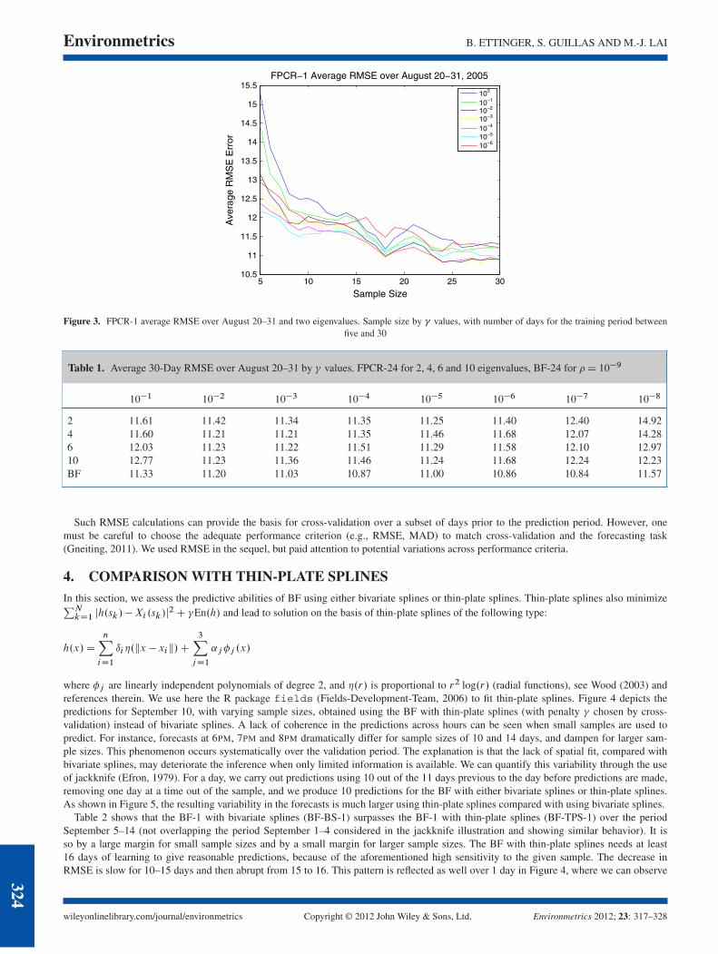
We show our numerical results using our FPCR approach to predict at the Atlanta station. In that setting, it is necessary to choose a numberof eigenvalues=eigenvectors to carry out the predictions. Hence, we have one additional tuning parameter in addition to the � values. Figure 3displays RMSEs for one such choice of two eigenvalues according to sample size. It shows that for FPCR-1, which uses 24 times less datapoints, but exactly at the hour of interest, the RMSEs are much larger but decrease steadily from these large values and reach lower valuesthan FPCR-1 after around 20 days. Hence, FPCR-1 is more tailored to the problem, but requires more days.

We considered 2, 4, 6 and 10 eigenvalues only, as forecasts were not improved by employing more than 10 eigenvalues. The tablesof RMSEs ranked by size of the learning period, for 2, 4, and 6 eigenvalues, are not displayed here, but show similar behavior. Table 1summarizes RMSEs for these various choices for FPCR-24 and provides a comparison with BF-24 for a sample size of 30 days.


323


5 10 15 20 25 3010.5

11

11.5

12

12.5

13

13.5

14

14.5

15

15.5FPCR−1 Average RMSE over August 20−31, 2005

Sample Size

Ave

rage

RM

SE

Err

or

100

10−1

10−2

10−3

10−4

10−5

10−6

Figure 3. FPCR-1 average RMSE over August 20–31 and two eigenvalues. Sample size by � values, with number of days for the training period betweenfive and 30

Table 1. Average 30-Day RMSE over August 20–31 by � values. FPCR-24 for 2, 4, 6 and 10 eigenvalues, BF-24 for �D 10�9

10�1 10�2 10�3 10�4 10�5 10�6 10�7 10�8

2 11.61 11.42 11.34 11.35 11.25 11.40 12.40 14.924 11.60 11.21 11.21 11.35 11.46 11.68 12.07 14.286 12.03 11.23 11.22 11.51 11.29 11.58 12.10 12.9710 12.77 11.23 11.36 11.46 11.24 11.68 12.24 12.23BF 11.33 11.20 11.03 10.87 11.00 10.86 10.84 11.57

Such RMSE calculations can provide the basis for cross-validation over a subset of days prior to the prediction period. However, onemust be careful to choose the adequate performance criterion (e.g., RMSE, MAD) to match cross-validation and the forecasting task(Gneiting, 2011). We used RMSE in the sequel, but paid attention to potential variations across performance criteria.

4. COMPARISON WITH THIN-PLATE SPLINESIn this section, we assess the predictive abilities of BF using either bivariate splines or thin-plate splines. Thin-plate splines also minimizePNkD1 jh.sk/�Xi .sk/j

2C �En.h/ and lead to solution on the basis of thin-plate splines of the following type:

h.x/D

nXiD1

ıi.kx � xik/C

3XjD1

˛j�j .x/

where �j are linearly independent polynomials of degree 2, and .r/ is proportional to r2 log.r/ (radial functions), see Wood (2003) andreferences therein. We use here the R package fields (Fields-Development-Team, 2006) to fit thin-plate splines. Figure 4 depicts thepredictions for September 10, with varying sample sizes, obtained using the BF with thin-plate splines (with penalty � chosen by cross-validation) instead of bivariate splines. A lack of coherence in the predictions across hours can be seen when small samples are used topredict. For instance, forecasts at 6PM, 7PM and 8PM dramatically differ for sample sizes of 10 and 14 days, and dampen for larger sam-ple sizes. This phenomenon occurs systematically over the validation period. The explanation is that the lack of spatial fit, compared withbivariate splines, may deteriorate the inference when only limited information is available. We can quantify this variability through the useof jackknife (Efron, 1979). For a day, we carry out predictions using 10 out of the 11 days previous to the day before predictions are made,removing one day at a time out of the sample, and we produce 10 predictions for the BF with either bivariate splines or thin-plate splines.As shown in Figure 5, the resulting variability in the forecasts is much larger using thin-plate splines compared with using bivariate splines.

Table 2 shows that the BF-1 with bivariate splines (BF-BS-1) surpasses the BF-1 with thin-plate splines (BF-TPS-1) over the periodSeptember 5–14 (not overlapping the period September 1–4 considered in the jackknife illustration and showing similar behavior). It isso by a large margin for small sample sizes and by a small margin for larger sample sizes. The BF with thin-plate splines needs at least16 days of learning to give reasonable predictions, because of the aforementioned high sensitivity to the given sample. The decrease inRMSE is slow for 10–15 days and then abrupt from 15 to 16. This pattern is reflected as well over 1 day in Figure 4, where we can observe324



Figure 4. Prediction using brute force with thin-plate spline (BF-TPS), over Sept 10, with varying sample sizes for the learning periods prior to predictions

Sept 1 , sample size: 10

hour

ozon

e

5 10 15 20

020

4060

8010

0


hour

ozon

e


hour

ozon

e

5 10 15 20

020

4060

8010

0

5 10 15 20

020

6040

8010

0

5 10 15 20

020

4060

8010

0


hour

ozon

e

Figure 5. Brute force jackknife predictions (sample size 10, after leaving one out of 11), with bivariate splines (green), thin-plate splines (red) and theobserved ozone values (black) over September 1–4

a sudden improvement in predictive power for the morning (mean level) as well as the afternoon (large reduction in variability); the possibleexplanation for such sensitivity may be the non-linear nature of the thin-plate splines fitting compared with bivariate splines fitting. Table 2also shows the advantage of using 24 h when computing the estimate of g: one does not need a large number of days to be able to producereasonable predictions. However, the drawback of this feature is that when sample size increases, the predictions are made using too muchaveraging, compared with the tailored 1-h-based version, as seen clearly when comparing the variation of RMSEs with sample size forBF-BS-24 and BF-BS-1. To compensate for larger instability when using smaller sample size in BF-BS-1 and FPCR-1, we increased thepenalty up to � D 1 to obtain good predictions.

Thin-plate splines are globally supported, so that large scale influences can occur in the fit with no respect of boundaries and sharp vari-ations. Bivariate splines are locally supported and can fit in any geometry of polygonal domain of interest. As a result, bivariate splinesare more likely to better represent local variations. Furthermore, the computational cost of using radial functions of the kind r2 log.r/is large due to numerical approximations in the integrals used to derive scalar products, whereas bivariate splines are merely polyno-mials for which immediate and exact results for integrals can be obtained. We noticed differences of several orders of magnitude inour particular computer set-up between bivariate splines and thin-plate splines. To overcome the difficulty of numerical approximations,Reiss and Ogden (2010) used another basis of radial functions: radial cubic B-splines over compact domains for a neuroimaging application.


325


Table 2. Average RMSEs of brute force (BF) with thin-plate splines (BF-TPS), BF-24 with bivariate splines�� D 10�4

�, BF-1 with

bivariate splines (� D 1), FPCR-24 with bivariate splines�� D 10�4

�, FPCR-1 with bivariate splines (� D 1), VAR-space, VAR-time,

over Sept 5–14 (10 day-long validation period) with sample sizes from 10 to 17 days

BF-TPS-1 BF-BS-24 BF-BS-1 FPCR-24 FPCR-1 VAR-space VAR-time

10 19.75 13.68 14.58 9.82 10.08 3:07� 108 4:87� 109

11 19.46 13.58 13.61 9.91 9.98 50.78 111.7312 19.21 13.22 12.70 9.91 9.94 33.18 37.5413 18.76 13.03 12.12 9.90 9.99 27.70 28.3614 18.32 12.94 11.52 9.89 9.87 23.41 40.7815 18.36 13.15 11.30 9.91 9.74 18.80 23.1616 12.48 12.95 11.05 9.92 9.82 20.40 20.5117 12.08 12.55 10.98 9.85 9.80 19.79 17.77

BF, brute force; TPS, thin-plate splines; BS, bivariate splines; FPCR, functional principal component regression; VAR, vectorautoregression.

However, these compactly supported splines do not possess optimal approximation properties, so their use may be restricted to samplelocations that are numerous and spatially covering the domain of interest, as in neuroimaging.

5. COMPARISON WITH THE VECTOR AUTOREGRESSION MODELIn Table 2, we compare the performance of our functional approach with a standard multivariate time series approach: the vector autore-gression model (VAR). We use the R package vars (Pfaff, 2008) with the default settings. We first select each vector of EPA stations inthe Southeast at a selected hour. There are 210 locations in our data set, and fitting the VAR requires at least 210 observations, so we cannotuse a model for each hour of the day as for BF-1 and FPCR-1. Therefore, we need to make use of all the previous hours in the 10–17-daysamples to have enough information to fit the VAR. To make a prediction using 10 days of learning for September 10, we are using a samplesize of 240 h, which is the same as in the BF=FPCR-24 models.

The next challenge in employing the VAR model is to impute a few missing data. To do so, we use either the spatial average over allavailable stations at the time when the observation is missing or the average value over all available observations at the same hour andat the same location where the data is missing. We denote these methods VAR-space and VAR-time in Table 2. Note that bivariate splinemethods do not suffer from these imputation problem as they naturally include an excellent interpolation step. We could have employedthis step in the VAR-space to impute these few missing values, but this was unlikely to significantly change the VAR predictions, and westuck to the standard VAR approach. Finally, because observations are rounded to the next integer by the EPA, many of the columns in theobservations are collinear, so we add negligible normally distributed random numbers with mean zero and standard deviation 0.01 to eachobservation to make the system solvable (correcting any values that becomes negative). The VAR models have huge errors for the 10-daysample size because the system is nearly collinear. However, we do see a decrease in errors as the sample size increases. Nevertheless, bothVAR approaches yield RMSEs around 40–100% higher than the BF and FPCR for the maximum sample size of 17 days considered here.

6. EFFECT OF TRIANGULATIONUnsurprisingly, preliminary analysis showed that large scale triangulations (such as the entire continental USA) do not produce goodforecasts as these spatial scales are producing spurious effects. Indeed, the chemistry and transport occur only at a regional scale on the24-h-ahead horizon. Hence, we only considered triangulations (Figure 1) over the Southeast USA to carry out statistical inference. We werenot able to draw a conclusion in terms of which one is the best as none of these three triangulations is consistently better than the othersacross the days of the validation period. Obviously, there is an infinite number of triangulations for this region. Finding an optimal triangula-tion for our purpose is very interesting and could lead to even better predictive abilities. It seems to be better to use a triangulation dependenton the geography as one wants to borrow strength spatially in a meaningful manner. For example, the ridges of mountains should be edgesof the triangulation; cities should be taken into account as predictions, for instance by putting them at the vertices of the triangulation. Thisinvestigation is beyond the scope of this paper.

7. CONCLUSIONS AND FUTURE RESEARCHThe BF method works very well for Atlanta. The predictions are consistent for various learning periods and the predictions are close to theexact measurements. Using the first two eigenvalues or more, FPCR also works very well. It is hard to say which one is better in general.However, on average, FPCR seems to slightly outperform BF in our example as it requires a smaller sample size to be efficient. Morenumerical evidence for the ozone concentration prediction at Atlanta on the basis of BF and FPCR can be found in Ettinger (2009).326



Overall, we recommend BF because it is simpler than FPCR, which requires some expert knowledge about how many eigenvalues areneeded for the best prediction. In our examples, we observed the decay of the eigenvalues, and often could not find an abrupt fall, also calleda knee, if the values of all eigenvalues are plotted on a normal scale. When plotted on a logarithmic scale, each of the eigenvalues (in the first10 of them) has a knee. It is hard to decide which one is the right knee. Determination of how many eigenvalues for the best prediction is notan easy task and requires further study. Yuan and Cai (2010) showed not only that the FPCR requires additional assumptions to be valid, butthat on well-designed simulations, predictions given by BF, with penalty � chosen with cross-validation, compares favorably with the FPCRfrom Hall and Horowitz (2007). However, if one has information about the principal components, or if the situation is made easy for theirestimation, it may be possible for FPCR to outperform BF in these cases. A reasonably accurate estimation of principal components mightexplain why this occurred in our example over the prediction period September 5–14. Finally, Ferraty et al. (2011) considered pre-smoothingfor FPCR, that is the perturbation of the normal equation �g D� at the beginning of the analysis. It seems to significantly improve the FPCRwhen the sample size is small or the noise is large. One could expect our results to be enhanced accordingly with the use of presmoothing.

It is also interesting to study the ozone value prediction at other cities, for example, Boston, Cincinnati and others, see Ettinger (2009) formore details. The numerical results again show that BF is easy to use and performs well. We see that the quality of predictions reaches aplateau after a learning period of around 15 days. Although in theory we can predict better if we use a longer learning period, the numericalresults vary on the basis of our experiments. We also conducted experiments for predictions using bivariate splines of degree d bigger than5: we employed d D 6; 7; 8 and 9 (not reported here). The numerical results are broadly similar to the predictions using bivariate splines ofdegree d D 5.

The inclusion of covariates (e.g., meteorological or even chemistry-transport model predictions) can improve such purely statistical ozonepredictions (Damon and Guillas, 2002; Guillas et al., 2008). We showed here the abilities of our method with no covariates, with potentialgains from the use of this additional information. However, the treatment of covariates (themselves spatially distributed) in this spatial func-tional data context is challenging. One possibility is first to merely add a non-spatially varying average effect as a parametric component.Such semiparametric functional models are now well understood (Aneiros and Vieu, 2006). A better idea would be to fully integrate thefunctional covariates. Modeling and computational issues arise, and this is currently under investigation.

Crainiceanu and Goldsmith (2010) recently developed Bayesian approaches for functional data, including a specific treatment of FPCR.Uncertainties are naturally computed as a result. Such Bayesian methods would most probably improve the quantification of uncertainties.

When the overall geographical coverage of triangulation is reasonably small (the coarseness is another issue), the predictions are betterfor both BF and FPCR for our particular example. Indeed, one should restrict itself to regions for which the spatial variability, throughchemistry and transport, corresponds to the time scale of the prediction. As a result, larger regions, possibly the entire continental USA, maybe appropriate for predictions at longer horizons when larger scale transport is occurring. One can foresee adaptive triangulations that wouldsuit particular conditions. The major conclusion from our results earlier is that bivariate splines outperform thin-plate splines in this contextboth in precision and computing time, and would do even more when the domain shows further constraints such as mountains and sea-shorethat have a large impact on chemistry and transport owing to their local features. Such qualities are attractive in various settings where takingboundaries into account would help improve interpolation over thin-plate splines (Newlands et al., 2011). We believe that our method hasthe potential to be implemented for operational pollution forecasting as a result.

AcknowledgementsBree Ettinger is partially funded by MIUR Ministero dellIstruzione dellUniversitá e della Ricerca, FIRB Futuro in Ricerca research project“Advanced statistical and numerical methods for the analysis of high dimensional functional data in life sciences and engineering”. Prof. Laiand Dr. Guillas were partially funded by the London Mathematical Society for this work. Ming-Jun Lai is partly supported by the NationalScience Foundation under grant DMS-0713807.

REFERENCES

Aneiros G, Vieu P. 2006. Semi-functional partial linear regression. Statistics & Probability Letters 76(11): 1102–1110.Aneiros-Perez G, Cardot H, Estevez-Perez G, Vieu P. 2004. Maximum ozone concentration forecasting by functional non-parametric approaches.

Environmetrics 15: 675–685.Awanou G, Lai M-J, Wenston P. 2006. The multivariate spline method for numerical solution of partial differential equations and scattered data interpolation.

In Wavelets and Splines: Athens 2005, Chen G, Lai M-J (eds). Nashboro Press: Brentwood, TN; 24–74.Bell M, McDermott A, Zeger S, Samet J, Dominici F. 2004. Ozone and short-term mortality in 95 US urban communities, 1987–2000. Journal of the American

Medical Assoication 292(19): 2372–2378.Cai T, Hall P. 2006. Prediction in functional linear regression. Annals of Statistics 34(5): 2159–2179.Cardot H, Ferraty F, Sarda P. 1999. Functional linear model. Statistics & Probability Letters 45: 11–22.Cardot H, Ferraty F, Sarda P. 2003. Spline estimators for the functional linear model. Statistica Sinica 13: 571–591.Crainiceanu C, Goldsmith A. 2010. Bayesian functional data analysis using WinBUGS. Journal of Statistical Software 32(11): 1–33.Crambes C, Kneip A, Sarda P. 2009. Smoothing splines estimators for functional linear regression. Annals of Statistics 37(1): 35–72.Cressie N, Wikle CK. 2011. Statistics for Spatio–Temporal Data. Wiley: Hoboken, New Jersey.Damon J, Guillas S. 2002. The inclusion of exogenous variables in functional autoregressive ozone forecasting. Environmetrics 13: 759–774.Dou Y, Le N, Zidek J. 2010. Modeling hourly ozone concentration fields. Annals of Applied Statistics 4(3): 1183–1213.Efron B. 1979. Bootstrap methods: another look at the jackknife. Annals of Statistics 7(1): 1–26.Ettinger B. 2009. Bivariate splines for ozone density predictions. Ph.D. Thesis, University of Georgia.Ferraty F, González-Manteiga W, Martinez-Calvo A, Vieu P. 2011. Presmoothing in functional linear regression. Statistica Sinica 22: 69–94.Ferraty F, Vieu P. 2006. Nonparametric Functional Data Analysis: Theory and Practice, Springer Series in Statistics. Springer-Verlag: London.


327


Fields-Development-Team. 2006. Fields: tools for spatial data, Technical Report, National Center for Atmospheric Research, Boulder, CO, USA.Gneiting T. 2011. Making and evaluating point forecasts. Journal of the American Statistical Association 106: 746–762.Guillas S, Bao J, Choi Y, Wang Y. 2008. Statistical correction and downscaling of chemical transport model ozone forecasts over Atlanta. Atmospheric

Environment 42: 1338–1348.Guillas S, Lai M. 2010. Bivariate splines for spatial functional regression models. Journal of Nonparametric Statistics 22(4): 477–497.Hall P, Horowitz J. 2007. Methodology and convergence rates for functional linear regression. Annals of Statistics 35(1): 70–91.Lai M-J. 2008. Multivariate splines for data fitting and approximation. In Approximation Theory XII: San Antonio 2007, Neamtu M, Schumaker LL (eds).

Nashboro Press: Brentwood, TN; 210–228.Lai M-J, Schumaker L. 2007. Spline Functions over Triangulations. Cambridge University Press: Cambridge.Neidell M. 2010. Air quality warnings and outdoor activities: evidence from Southern California using a regression discontinuity design. Journal of

Epidemiology & Community Health 64(10): 921–926.Newlands NK, Davidson A, Howard A, Hill H. 2011. Validation and inter-comparison of three methodologies for interpolating daily precipitation and

temperature across Canada. Environmetrics 22(2): 205–223.Paciorek CJ, Yanosky JD, Puett RC, Laden F, Suh HH. 2009. Practical large-scale spatio–temporal modeling of particulate matter concentrations. Annals of

Applied Statistics 3(1): 370–397.Pfaff B. 2008. Analysis of Integrated and Cointegrated Time Series with R, 2nd ed. Springer: New York. ISBN 0-387-27960-1.Ramsay J, Silverman B. 2005. Functional Data Analysis. Springer-Verlag: New York, NY.Reiss P, Ogden R. 2010. Functional generalized linear models with images as predictors. Biometrics 66(1): 61–69.Wood SN. 2003. Thin plate regression splines. The Journal of the Royal Statistical Society, Series B (Statistical Methodology) 65(1): 95–114.Yuan C, Cai T. 2010. A reproducing kernel Hilbert space approach to functional linear regression. Annals of Statistics 38(6): 3412–3444.

328


Documents

Bivariate splines for ozone concentration forecastingmath.uga.edu/~mjlai/papers/EGL12.pdf · Research Article Environmetrics Received: 20 June 2011, Revised: 22 March 2012, Accepted: