Biota Sediment Accumulation Factors for Invertebrates ...rais.ornl.gov/documents/bjcor-112a1.pdf · Biota Sediment Accumulation Factors for Invertebrates: Review and ... Biota Sediment

BJC/OR-112

Biota Sediment Accumulation Factorsfor Invertebrates: Review and

Recommendations for the Oak Ridge Reservation

This document has been approvedfor release to the public. Date: 8/31/98

BJC/OR-112

Biota Sediment Accumulation Factors for Invertebrates: Review and

Recommendations for the Oak Ridge Reservation

Date Issued—August 1998

Prepared for theU.S. Department of Energy

Office of Environmental Managementunder budget and reporting code EW 20

BECHTEL JACOBS COMPANY LLCmanaging the

Environmental Management Activities at theEast Tennessee Technology Park

Oak Ridge Y-12 Plant Oak Ridge National LaboratoryPaducah Gaseous Diffusion Plant Portsmouth Gaseous Diffusion Plant

under contract DE-AC05-98OR22700for the

U.S. DEPARTMENT OF ENERGY

iii

PREFACE

The purpose of this report is to acquire contaminant uptake data from published andunpublished literature, develop and present biota-sediment accumulation factors and regressionequations for estimating chemical concentrations in benthic invertebrates for use on the Oak RidgeReservation, and compare these to contaminant uptake data for emergent adult insects. This workwas performed under Work break down Structure 1.4.12.2.3.04.05.03 (Activity Data Sheet 8304).The equations and biota-sediment accumulation factors presented in this report will facilitate theestimation of contaminant exposure experienced by wildlife consuming flying insects on the OakRidge Reservation. This report also provides a foundation for the process of developing bodyburden benchmarks for effects to benthic invertebrates and biota-sediment accumulation factors forfish. This report was originally issued as a draft under number ES/ER/TM-214.

iv

v

CONTENTS

PREFACE . . . . . . . . . . . . . . . . . . . . . . . . . . . . . . . . . . . . . . . . . . . . . . . . . . . . . . . . . . . . . . . . . . . . . . . . iii

TABLES . . . . . . . . . . . . . . . . . . . . . . . . . . . . . . . . . . . . . . . . . . . . . . . . . . . . . . . . . . . . . . . . . . . . . . . . . . vii

FIGURES . . . . . . . . . . . . . . . . . . . . . . . . . . . . . . . . . . . . . . . . . . . . . . . . . . . . . . . . . . . . . . . . . . . . . . . . . . ix

EXECUTIVE SUMMARY . . . . . . . . . . . . . . . . . . . . . . . . . . . . . . . . . . . . . . . . . . . . . . . . . . . . . . . . . . . xi

1. INTRODUCTION . . . . . . . . . . . . . . . . . . . . . . . . . . . . . . . . . . . . . . . . . . . . . . . . . . . . . . . . . . . . . . . . 1

2. MATERIALS AND METHODS . . . . . . . . . . . . . . . . . . . . . . . . . . . . . . . . . . . . . . . . . . . . . . . . . . . 22.1. LITERATURE REVIEW . . . . . . . . . . . . . . . . . . . . . . . . . . . . . . . . . . . . . . . . . . . . . . . . . . . . 22.2. MODEL DEVELOPMENT . . . . . . . . . . . . . . . . . . . . . . . . . . . . . . . . . . . . . . . . . . . . . . . . . . 6

2.2.1 Metals . . . . . . . . . . . . . . . . . . . . . . . . . . . . . . . . . . . . . . . . . . . . . . . . . . . . . . . . . . . . . . . . . 62.2.2 PCBs . . . . . . . . . . . . . . . . . . . . . . . . . . . . . . . . . . . . . . . . . . . . . . . . . . . . . . . . . . . . . . . . . . 7

2.3 VALIDATION . . . . . . . . . . . . . . . . . . . . . . . . . . . . . . . . . . . . . . . . . . . . . . . . . . . . . . . . . . . . . . 7

3. RESULTS . . . . . . . . . . . . . . . . . . . . . . . . . . . . . . . . . . . . . . . . . . . . . . . . . . . . . . . . . . . . . . . . . . . . . . . 83.1 MODELING RESULTS . . . . . . . . . . . . . . . . . . . . . . . . . . . . . . . . . . . . . . . . . . . . . . . . . . . . . . 8

4. DISCUSSION . . . . . . . . . . . . . . . . . . . . . . . . . . . . . . . . . . . . . . . . . . . . . . . . . . . . . . . . . . . . . . . . . . 26

5. RECOMMENDATIONS . . . . . . . . . . . . . . . . . . . . . . . . . . . . . . . . . . . . . . . . . . . . . . . . . . . . . . . . . 28

6. REFERENCES . . . . . . . . . . . . . . . . . . . . . . . . . . . . . . . . . . . . . . . . . . . . . . . . . . . . . . . . . . . . . . . . . 29

APPENDIX A: PROCEDURE FOR CALCULATION OF PREDICTION LIMITS FORESTIMATES GENERATED BY THE REGRESSION MODELS . . . . . . . . . . . . . . . . . . . . 33

vi

vii

TABLES

Table 1. Summary of Sources for Sediment and Invertebrate Concentration Data . . . . . . . . . . . 3Table 2. Summary statistics for literature-derived sediment-invertebrate accumulation

factors . . . . . . . . . . . . . . . . . . . . . . . . . . . . . . . . . . . . . . . . . . . . . . . . . . . . . . . . . . . . . . . 9Table 3. Summary results for regression analyses of log-transformed sediment and

invertebrate metal concentrations reported in the literature . . . . . . . . . . . . . . . 12a

Table 4. Quality of “Most Likely” estimation methods as determined by the proportional deviation (PD) of the estimated values from measured values . . . . . . . . . . . . . 20a

Table 5. Quality of conservative estimation methods as determined by the proportional deviation (PD) of the estimated values from measured values . . . . . . . . . . . . . 25a

viii

ix

FIGURES

Figure 1. Linear and Log-log scatterplots of arsenic concentrations in sediment, benthic invertebrates, and emergent adult insects. The regression lines are based on all of the available data for benthics (depurated and non-depurated). . . . . . . . 14

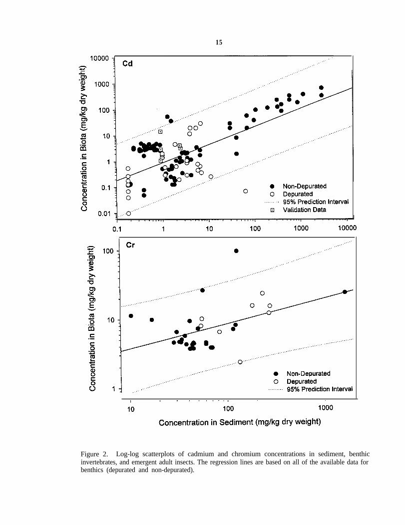
Figure 2. Log-log scatterplots of cadmium and chromium concentrations in sediment, benthic invertebrates, and emergent adult insects. The regression lines are based on all of the available data for benthics (depurated and non-depurated). . . . . . . . . . . . . . . . . . . . . . . . . . . . . . . . . . . . . . . . . . . . . . . . . . . . . . . 15

Figure 3. Log-log scatterplots of copper and mercury concentrations in sediment, benthic invertebrates, and emergent adult insects. The regression lines are based on allof the available data for benthics (depurated and non-depurated). . . . . . . . . . . 16

Figure 4. Log-log scatterplots of nickel and lead concentrations in sediment, benthic invertebrates, and emergent adult insects. The regression lines for lead are based on all of the available data for benthics (depurated and non-depurated). Separate regression lines are presented for nickel in depurated and non-depurated benthics. . . . . . . . . . . . . . . . . . . . . . . . . . . . . . . . . . 17

Figure 5. Log-log scatterplots of zinc and PCB concentrations in sediment, benthic invertebrates, and emergent adult insects. The regression lines for zinc arebased on all of the available data for benthics (depurated and non-depurated). The regression lines for PCBs are based on the data for benthics. . . . . . . . . . . 18

Figure 6. Cumulative distributions of arsenic and cadmium BSAFs for benthic invertebrates (depurated and non-depurated) and emergent adult insects. . . . . 21

Figure 7. Cumulative distributions of copper and mercury BSAFs for benthic invertebrates (depurated and non-depurated) and emergent adult insects. . . . . . . . . . . . . . . . . 22

Figure 8. Cumulative distributions of lead and zinc BSAFs for benthic invertebrates (depurated and non-depurated) and emergent adult insects. . . . . . . . . . . . . . . . . 23

Figure 9. Cumulative distributions of PCB BSAFs for benthic invertebrates (depurated and non-depurated) and emergent adult insects. . . . . . . . . . . . . . . . . . . . . . . . . . . 24

Figure 10. Log-log scatterplot of PCB concentrations in sediment and emergent adult insects. The regression lines are based on the available data for emergent adults. . . . . . . . . . . . . . . . . . . . . . . . . . . . . . . . . . . . . . . . . . . . . . . . . . . . . . . . . . . . . . . 26

x

xi

EXECUTIVE SUMMARY

Benthic invertebrates, fish, and flying insectivores are important assessment endpoints for theevaluation of ecological risks at aquatic sites on and near the Oak Ridge Reservation. One of theprimary exposure pathways for these organisms is the consumption of contaminated food.Deposited sediments often act as a local sink for contaminants, which may increase the contaminantexposure for sediment-associated biota that indiscriminately ingest sediment particles whileforaging. Benthic invertebrates are an important food source for fish and some terrestrial wildlife.Flying insectivores such as swifts, swallows, and bats, including the threatened and endangered greybat, forage over water and consume adult insects that have aquatic larval stages (e.g., mayflies andmidges). Therefore, larval infauna can be an important vector for the movement of chemicals outof sediment deposits and into the water column and terrestrial foodchains.

The simplest method for estimating contaminant loads in biota is the use of accumulation factors(AFS). AFs consist of ratios of the concentration of a given contaminant in biota to that in anabiotic medium. For the evaluation of sediments, this is commonly presented as the biota-sedimentaccumulation factor (BSAF). The concentration in biota may be estimated by multiplying thesediment concentration by the BSAF. This method is particularly useful for ecological riskassessments because ambient media concentrations are usually available; ambient media data areneeded for the site characterization and human health assessments typically conducted inconjunction with ecological assessments. Concentrations in most biota are used only for theecological risk assessment and are frequently not available, especially for screening levelassessments. Separate BSAFs are required for each chemical because they are empirically derived,rather than based on general physico-chemical parameters. Bioavailability of contaminants foruptake can be influenced by sediment conditions including the pH and the amount of acid-volatile-sulfide that is available for complexing with divalent metals (e.g., Cd, Cu, Pb, Ni, and Zn).

The purpose of this report is to acquire contaminant uptake data from published and unpublishedliterature, develop and present BSAFs and regression equations for estimating chemicalconcentrations in benthic invertebrates for use on the Oak Ridge Reservation, and compare theseto contaminant uptake data for emergent adult insects. The equations and BSAFs presented in thisreport will facilitate the estimation of contaminant exposure experienced by wildlife consumingflying insects on the Oak Ridge Reservation. This report also provides a foundation for the processof developing body burden benchmarks for effects to benthic invertebrates and BSAFs for fish.

xii

1

1. INTRODUCTION

Benthic invertebrates, fish, and flying insectivores are important assessment endpoints for theevaluation of ecological risks at aquatic sites on and near the ORR. One of the primary exposurepathways for these organisms is the consumption of contaminated food. Deposited sediments oftenact as a local sink for contaminants, which may increase the contaminant exposure for sediment-associated biota that indiscriminately ingest sediment particles while foraging. Benthicinvertebrates are an important food source for fish and some terrestrial wildlife. Flying insectivoressuch as swifts, swallows, and bats, including the Threatened and Endangered grey bat, forage overwater and consume adult insects which have aquatic larval stages (e.g., mayflies and midges).Hence, larval infauna can be an important vector for the movement of chemicals out of sedimentdeposits and into the water column and terrestrial foodchains(Currie et al. 1997, Froese et al. 1998,and Larsson 1984)

Concentrations of bioavailable contaminants in sediment are needed to evaluate foodchaintransfer and the potential toxicity of sediment contaminants. The bioavailable fraction can bemeasured directly by collecting and analyzing benthic invertebrates or it can be estimated.Contaminant concentrations in flying insects are needed to estimate the magnitude of contaminantexposure that flying insectivores may experience at a contaminated site. These concentrations alsomay be acquired either by direct measurement of contaminants in flying insects or by estimation.Direct measurement is the preferred approach because it contributes the least uncertainty toexposure estimates. That is, it provides information on the actual contaminant loading in on-sitebiota. However, direct measurement of contaminant concentrations in biota may not be feasiblebecause of a lack time, personnel, or finances to support field sampling. When direct measurementof contaminants in biota is not possible, estimation is the only alternative.

Contaminant concentrations in biota may be estimated using a variety of methods, ranging fromcomplex mechanistic process models to simple accumulation factors. While mechanistic processmodels for the estimation of contaminant concentrations in biota may give more accurate estimates,they require information which is not generally available for a risk assessment. An example of amechanistic contaminant uptake model for fish is presented in Thomann et al. (1992).

The simplest method for estimation of contaminant loads in biota is the use of accumulationfactors (AFs). AFs consist of ratios of the concentration of a given contaminant in biota to that inan abiotic medium. For the evaluation of sediments this is commonly presented as the biota-sediment accumulation factor (BSAF). The concentration in biota may be estimated by multiplyingthe sediment concentration by the BSAF. This method is particularly useful for ecological riskassessments because ambient media concentrations are usually available; ambient media data areneeded for the site characterization and human health assessments typically conducted inconjunction with ecological assessments. Concentrations in most biota are used only for theecological risk assessment and are frequently not available, especially for screening levelassessments. Separate BSAFs are required for each chemical because they are empirically derived,rather than being based on generalizable physico-chemical parameters. Bioavailability ofcontaminants for uptake can be influenced by sediment conditions including the pH and the amountof acid-volatile-sulfide (AVS) that is available for complexing with divalent metals (i.e., Cd, Cu,Pb, Ni, and Zn).

The use of uptake factors, including BSAFs, depends on the assumption that the concentrationof chemicals in organisms is a linear no threshold function of the concentration in sediment. This

2

will not be the case if uptake or depuration of the chemical in question is well-regulated by theorganism, either because it is an essential nutrient or because it is a toxicant for which the organismhas inducible mechanisms for metabolism or excretion. Well regulated chemicals will have nearlyconstant concentrations regardless of sediment concentrations, at least within the effectiveconcentration range for the regulating mechanism. Various complex patterns also are possible dueto lack of induction at low concentrations, saturation kinetics at high concentrations, toxicity at highconcentrations, or other processes. Despite these conditions that lead to violation of theassumptions, accumulation factors are commonly used in risk assessments.

The purpose of this report is to acquire contaminant uptake data from published and unpublishedliterature, develop and present BSAFs and regression equations for estimating chemicalconcentrations in benthic invertebrates for use on the ORR, and compare these to contaminantuptake data for emergent adult insects. Sediment to emergent adult BSAFs and regression equationsalso are included if sufficient data are available (i.e., PCBs). The equations and BSAFs presentedin this report will facilitate the estimation of contaminant exposure experienced by wildlifeconsuming flying insects on the ORR. This report also provides a foundation for the process ofdeveloping body burden benchmarks for effects to benthic invertebrates and BSAFs for fish.

2. MATERIALS AND METHODS

2.1. LITERATURE REVIEW

To determine how contaminant uptake varies across locations, contaminant levels, and sedimentconditions, we performed a literature search for studies reporting chemical concentrations in co-located sediment and invertebrate samples. Literature was reviewed for eight chemicals: arsenic,cadmium, chromium, copper, mercury, lead, nickel, zinc, and PCBs (Table 1). Sediment andinvertebrate contaminant concentration data were extracted from each paper and used to calculatean accumulation factor.

Data were recorded for freshwater invertebrates, with particular emphasis on invertebrates thathave terrestrial adult life stages (e.g., mayflies) or are generally consumed by fish (e.g., amphipodsand tubificid worms). Data for marine and estuarine biota were not included in this evaluation.BSAFs and regression equations for metals were calculated on a dry weight basis. Biotaconcentrations reported in the literature only on a wet weight basis (e.g., mg Cu/kg fresh tissue)were included only if a wet-weight to dry-weight conversion factor also was presented. For PCBs,the BSAFs and regression equations were derived using sediment concentrations normalized toorganic carbon content (e.g., ug PCB/g organic carbon) and organism concentrations normalizedto lipid content (e.g., ug PCB/g lipid). Reported PCB concentrations were included only if organiccarbon and lipid content values were presented. Biota concentrations presented only on a perorganism basis (e.g., mg Cu/individual) were not included. Some studies were designed to elucidatemechanisms of uptake by using non-standard extraction methods. Only the results for methodstypically used in environmental assessments

Table 1. Summary of Sources for Sediment and Invertebrate Concentration Data

3

Analytes Study Locations No. Sample Organisms Depurated ReferenceLocations

Benthic Organisms

Cd, Cr, Cu, Ni, Pb, Zn Wisconsin 3 Yes Ankley et at. 1944Oligochaetes (Lumbriculus variegatus)

Cd, Hg Upper Miss. River 12 No Beauvais et al. 1995Mayfly (Hexagenia spp.)

Cu, Pb, Zn Salmon River 2 Yes Bindra & Hall 1977, cited inOligochaetes (Limnodrilus hoffmeistri,Tubifex tubifex) Chapman et al. 1979

As, Cd, Cu, Pb, Zn Montana 9 Caddisfly, Mayfly, Stonefly, Hemiptera No Cain et al. 1992(Various species)

Cd, Cu, Pb Montana 5 Caddisfly, Stonefly (Various species) Yes Cain et al. 1995

Cd East River, 9 Yes Carlson et al. 1991Pequayman Lake, West Bearskin Lake

Oligochaetes (Lumbriculus variegatus)

Cu, Hg, Ni, Pb, Zn Canada 2 Yes Chapman et al. 1979Oligochaetes (Limnodrilus hoffmeistri,Tubifex tubifex)

As, Cd, Cu, Hg, Pb, Zn S. Africa 1 Oligochaetes & Composite No Greichus et al. 1978

As, Cd, Cu, Zn Quebec 1 Yes Hare et al. 1989Mayfly (Hexagenia limbata)

Cd, Cu, Zn Quebec 3 Alderfly, Mayfly, Phantom midge, and Yes Hare & Campbell 1992Midge (Sialis spp., Hexagenia limbata,Chaorobus punctipennis, Chironomussp., Glyptotendipes sp., Procladiusspp.)

Cd, Cu, Pb, Zn Laboratory 2 No Harrahy & Clements 1997a Midge (Chironomus tentans)

As, Cd, Cu, Pb, Zn Montana 7 No Ingersoll et al. 1994Amphipod (Hyallela azteca)

Table 1. (Continued)

4


Cd, Cr, Cu, Ni, Pb, Zn Maryland 20 Dragonfly (Various species) & No Karouna-Renier 1995; MS ThesisCompositeb

As, Cd, Cr, Cu, Ni, Pb, Zn Lake Ontario 5 Oligochaetes Yes Krantzberg 1994

Pb Illinois 3 Damselfly, Mayfly, Midge, Moth Flies, No Leland & McNurney 1974Oligochaetes (Anisoptera, Hexagenialimbata, Chirnomidae, Psychodidae,Tubificidae and Oligochaeta)

Cd, Cr, Cu, Ni, Pb, Zn Illinois 1 No Mathis & Cummings 1973Oligochaetes (Limnodrilus hoffmeistri,Tubifex tubifex)

Cu, Pb, Zn Oklahoma 1 Composite No Namminga et al. 1974b

As, Cd, Cu, Pb, Zn Montana 6 Composite No Poulton et al. 1995b

Cr, Zn North Carolina 8 Composite No Shuman et al. 1977b

Cd, Cu, Pb, Zn Netherlands 1 Amphipod, Caddisfly, Dragonfly, Yes Timmermans et al. 1989Hemiptera, Isopod, Midge (Variousspecies)

PCBs Wisconsin 1 N/A Ankley et al. 1992Oligochaetes (Lumbriculus sp. andLumbriculus variegatus)

c

PCBs Michigan 1 N/A Drouillard et al. 1996Mayfly (Hexagenia limbata) c

PCBs Ontario 1 N/A Gobas et al. 1989Mayfly (Hexagenia limbata) c

PCBs Lake Erie 1 Zebra mussel, Caddisfly, Amphipod, N/A Morrison et al. 1996and Crayfish (Dreissena polymorpha,Hydropsyche alterans, Gammarusfasciatus, and Orconectec propinquus)

c

Table 1. (Continued)

5


PCBs Lake Ontario 6 N/A Oliver 1987Oligochaetes (Limnodrilus hoffmeistriand Tubifex tubifex)

c

PCBs Netherlands 1 N/A van der Oost et al. 1988Mollusc and Crustaceans (Dreisenapolymorpha and various species)

c

Emergent Adults

Cd Ontario 1 N/A Currie et al. 1997Dragonfly and Mayfly (Odonata spp.And Hexagenia spp.)

d

As, Pb, Hg, Zn Tennessee 3 N/A Department of Energy 1996Mayfly (Hexegenia rigida) d

Cd, Cu, Zn Michigan 2 Midge (Chironomidae spp.) N/A Young and Harvey 1988d

PCBs Michigan 1 Emergent Insects (Various species) N/A Froese et al. 1998d

PCBs Laboratory 9 N/A Larsson 1984a Midge (Chironomus plumosus) d

Results from a spiked-sediment bioassay.a

Composite of various benthic invertebrates analyzed togetherb

Not Applicable for analyses of PCBs, which are normalized to the organism lipid content. c

Not applicable to analyses of emergent adults.d

6

(e.g., hot acid extraction of sediment metals) were used from such studies. Unfortunately, manypotentially useful studies had to be eliminated for the aforementioned reasons.

Metal concentrations in biota were recorded as “depurated” for organisms that were allowedto purge their gut contents in clean water or sediment or were dissected to remove their gut contents.Biota concentrations that included gut contents were recorded as “Non-Depurated.” Gut contentsare presumed to be a negligible source of error for lipid-normalized organic chemical concentrationsand were not explicitly accounted for in this evaluation.

Other relevant sediment and biota characteristics also were recorded. Sediment characteristicsincluded percent sand, silt, and clay; percent organic carbon content; AVS and simultaneouslyextracted metal (SEM) concentrations; and interstitial water concentrations. Biota characteristicsincluded the scientific and common name; life stages analyzed (larvae, pupae, or adult); feedingbehavior (water column filter feeders, sediment ingesters, etc.); organism habits and habitats (e.g.,burrowing in sediment depositional areas); and concurrently measured adverse effects (e.g., survivalor density). These sediment and biota characteristics were recorded for future use and were notexplicitly incorporated into the current evaluation.

2.2. MODEL DEVELOPMENT

2.2.1 Metals

BSAFs were calculated for each analyte, site, and species combination reported in a givenstudy. Replicate sediment and biota measurements for a site and species combination were averagedtogether. Most of the available studies reported uptake from a limited number of locations orrepresented only a small range of sediment concentrations. However, a broad range of sedimentconcentrations are needed to best evaluate the relationship between concentrations of contaminantsin sediment and those in benthic invertebrates. To that end, biota and sediment concentrations andthe resulting BSAFs for each analyte were placed in one of two groups: those for which depuratedorganisms were analyzed (“Depurated”) and those for which undepurated organisms were analyzed(“Non-Depurated”). BSAFs and accumulation models were subsequently developed for each groupindependently and for the entire data set (“All”).

Summary statistics were calculated for BSAFs for each chemical and data set combination.The Shapiro-Wilk test (PROC UNIVARIATE; SAS Inst. Inc. 1988a) was applied to theuntransformed and log-transformed BSAFs for each analyte to determine if the distribution of theBSAFs was normal or log-normal, respectively. Distributions were fit only for data sets with fouror more BSAFs. A uniform distribution (i.e., all values are equally likely) was assumed if therewere fewer than four BSAFs.

Regression analyses of the sediment and biota data also were performed for each chemical anddata set combination. Because data concerning the number of individuals included in compositesor means were not available for all observations, no weighting of observations was applied. Datawere evaluated graphically and considered to be best fit by a power model. This is consistent withevaluations reported elsewhere (Sample et al. 1997). The power model of the form

y = a(x) (1)b

7

was linearized for the regression analyses by log-transforming the sediment and biotaconcentrations. The transformed model is:

log(y) = a! + b log(x). (2)

where:

y = chemical concentration in the organism (mg/kg dry wt.)x = chemical concentration in sediment (mg/kg dry wt.)a! = log-transformed y interceptb = slope

2.2.2 PCBs

BSAFs were calculated for each site and species combination reported in a given study.Replicate measurements for a site and species combination were averaged together. Most of theavailable studies were designed to evaluate the uptake of non-ionic organic chemicals relative tochemical-specific characteristics (e.g., the organic carbon-partitioning coefficient). Such studiesgenerally presented concentrations of individual congeners. The reported coongener concentrationswere summed to obtain a total PCB concentration, because congener-specific data are not typicallyavailable for screening ecological risk assessments.

Summary statistics were generated for the PCB BSAFs. As with the BSAFs for metals, theShapiro-Wilk test (PROC UNIVARIATE; SAS Inst. Inc. 1988a) was applied to the untransformedand log-transformed BSAFs to determine if the distribution of the BSAFs was normal orlog-normal, respectively.

Regression analyses of the sediment and biota data also were performed for PCBs using thelinearized power model (Eq. 2). Where “y” is the PCB concentration in the organism (ug/g lipid)and “x” is the PCB concentration in sediment (ug/g organic carbon)

2.3 VALIDATION

BSAFs and regression models developed from the benthos data were applied to the sedimentconcentration data in the validation dataset, and estimated contaminant concentrations in emergentadult insects were generated. “Most likely” estimates were generated using the median BSAF andthe regression model. Conservative estimates for use in screening assessments were generated usingthe 90th percentile BSAF and the upper 95% prediction limit (95% UPL) for the regression models.The 95% UPL was calculated according to Dowdy and Wearden (1983) [Note: methods andparameters for calculating the 95% UPL are presented in Appendix A].

The appropriateness and accuracy of the estimation methods was evaluated for each analyte,data set, and estimation method. Differences between estimated and measured concentrations inemergent adults were evaluated using Wilcoxon signed-rank tests (PROC UNIVARIATE; SAS Inst.Inc. 1988a). Differences were considered significant if p(H =0)#0.05. Relative accuracy and0

quality of different estimation methods were evaluated by calculating the proportional deviation ofthe estimate from the measured value:

PD = (Mi - Ei) / Miwhere

8

PD= proportional deviationMi = measured concentration in emergent adult insects at sediment concentration (i)Ei = estimated concentration in emergent adult insects at sediment concentration (i)

Negative values for PD indicate overestimation while positive PD values indicateunderestimation. The percentage of estimated values that exceeded their corresponding measuredvalue was also tabulated for each chemical and estimation method. Relative quality of the “MostLikely” estimation methods was evaluated by the following criteria:

1) median PD closest to 0 (indicates estimates center around measured values);2) PD with narrowest range (indicates relative accuracy of method); 3) percentage overestimation closest to 50% (indicates estimates center around measured values);4) difference between estimated and measured values not significantly different as determined by

Wilcoxon signed-rank tests.

Relative quality of conservative estimation methods was evaluated by

1) smallest, negative median PD value (indicates method overestimates while minimizing thedegree of overestimation);

2) PD with narrowest range (to minimize the degree of overestimation);

In addition to the use of PD values, the concentrations in emergent adult insects relative to thatof benthic organisms was evaluated graphically. Validation data (concentrations in adults andsediment) were included in the scatter plots of the model data (concentrations in benthos andsediment) to allow comparison of the ranges of sediment concentrations, the trends in biotaconcentrations relative to sediment concentrations, and the trends in observed adult concentrationsrelative to those predicted by the regression model. BSAFs for emergent adults and benthos alsowere plotted to allow comparison of the trends of predictions based on accumulation factors.

There was sufficient PCB validation data (ten observations) to develop a linear regressionequation for the log-transformed sediment and emergent adult concentrations. This model wascompared to regressions developed from the benthos data using the F-test procedure for comparingregression lines outlined in Draper and Smith (1981). Differences were considered significant ifp#0.05.

3. RESULTS

3.1 MODELING RESULTS

Summary statistics for the BSAFs for each chemical and data set combination are presentedin Table 2. Data sets for which the median BSAFs were less than 1 included the “All”

9

Table 2. Summary statistics for literature-derived sediment-invertebrate accumulation factors

Analyte Data Set N Mean Deviation m Median Percentile Maximum formed Values formed Values DistributionaStandard Minimu 90th Log-Trans- Log-Trans-

Mean of Deviation ofStandard

As All 55 0.329 0.597 0.018 0.143 0.690 4.330 -0.764 0.476 Lognormal

As Non-Dep. 49 0.240 0.236 0.018 0.127 0.675 0.889 -0.828 0.442 Lognormal

As Dep. 6 1.058 1.611 0.278 0.373 4.330 4.330 -0.245 0.457 Lognormalb

Cd All 120 2.822 5.227 0.001 0.600 7.990 41.550 -0.099 0.749 Lognormalb

Cd Non-Dep. 88 3.438 5.938 0.049 0.614 9.240 41.550 0.005 0.710 Lognormalb

Cd Dep. 32 1.126 1.362 0.001 0.459 3.073 4.878 -0.387 0.789 Lognormalb

Cr All 34 0.179 0.227 0.015 0.100 0.468 1.101 -0.941 0.390 Lognormal

Cr Non-Dep. 26 0.206 0.252 0.015 0.108 0.588 1.101 -0.883 0.396 Lognormal

Cr Dep. 8 0.090 0.055 0.018 0.083 0.186 0.186 -1.133 0.322 Normal b

Cu All 112 2.424 3.755 0.032 1.556 5.250 23.870 0.005 0.633 Lognormalb

Cu Non-Dep. 74 2.140 2.621 0.032 1.647 3.872 16.630 0.050 0.565 Lognormalb

Cu Dep. 38 2.976 5.318 0.047 0.661 7.957 23.870 -0.084 0.750 Lognormal

Hg All 15 1.422 0.940 0.286 1.136 2.868 3.981 0.074 0.275 Lognormal

Hg Non-Dep. 13 1.204 0.653 0.286 1.081 1.735 2.868 0.022 0.245 Lognormalc

Hg Dep. 2 2.837 1.619 1.692 2.837 3.981 3.981 0.414 0.263 Lognormalv

Ni All 26 0.857 1.230 0.055 0.486 2.320 5.746 -0.375 0.534 Lognormal

Table 2. (continued)

10

Analyte Data Set N Mean Deviation m Median Percentile Maximum formed Values formed Values DistributionaStandard Minimu 90th Log-Trans- Log-Trans-

Mean of Deviation ofStandard

Ni Non-Dep. 16 1.313 1.395 0.397 0.818 3.150 5.746 -0.024 0.329 Lognormal

Ni Dep. 10 0.129 0.059 0.055 0.134 0.214 0.237 -0.935 0.214 Normalc

Pb All 114 0.276 0.787 0.004 0.071 0.607 7.080 -1.069 0.575 Lognormalb

Pb Non-Dep. 83 0.331 0.915 0.004 0.066 0.946 7.080 -1.063 0.624 Lognormalb

Pb Dep. 31 0.129 0.132 0.009 0.080 0.326 0.503 -1.084 0.423 Lognormal

Zn All 112 3.092 3.335 0.026 1.936 7.527 14.512 0.160 0.622 Lognormalb

Zn Non-Dep. 84 3.473 3.577 0.026 2.330 8.465 14.512 0.229 0.610 Lognormalb

Zn Dep. 28 1.952 2.141 0.079 0.840 4.759 8.479 -0.047 0.622 Lognormal

PCBs (infauna) 16 9.016 12.796 0.739 4.670 21.886 51.313 0.652 0.530 LognormalModel

PCBs (adult) 10 37.193 19.118 11.176 36.215 64.122 67.132 1.508 0.261 NormallValidation

c

All = depurated and non-depurated invertebrates combined, Dep. = invertebrates depurated prior to analysis, Non-Dep. = invertebrates not depurated prior toa

analysis, Model = benthic invertebrates analyzed for PCBs, Validation = emergent adult insect analyzed for PCBs. p<0.05 for both normal and lognormal distributionsb

p>0.05 for both normal and lognormal distributionsc

11

and “Non-Depurated” data for As, Cd, Cr, Ni, and Pb and the “Depurated” data for Cu and Zn. Thisindicates that the invertebrates analyzed in most of the evaluated studies did not accumulate theseanalytes to levels greater than those measured in the associated sediments. The maximum BSAFsfor Cr, Ni, and Pb in depurated organisms also were less than 1. However, at least one reportedBSAF was greater than 1 for all chemicals. The maximum BSAF for all metals was 23.9 for Cu indepurated organisms. The maximum BSAF for PCBs were 51.3 for benthos and 67.1 for emergentadults. The minimum BSAF for all analytes was 0.001 for Cd in depurated organisms.

For three metals (As, Hg, and Pb) the median BSAF for depurated organisms was greater thanthe median BSAF for non-depurated organisms. This is consistent with expected results for Hg,which should accumulate in the tissue to concentrations higher than those found in sediment. ForAs and Pb, it is more likely because of sampling error (measured sediment concentrations notrepresentative of organism exposures) or differences in the taxa included in the two data sets. Themedian BSAF for all organisms was between the median BSAFs for each of the individual data setsfor all metals. The 90th percentile BSAF for three metals (As, Cu, and Hg) in depurated organismswas greater than that for the non-depurated organisms.

The distributions of BSAFs for most analytes and data set combinations (22 of 26) were betterdescribed by a lognormal distribution than by a normal distribution. The three BSAF distributionsthat were better described by a normal distribution were also not significantly different (p < 0.05)from a lognormal distribution. Only one distribution better described by a lognormal distributionwas also not significantly different (p < 0.05) from a normal distribution. Each of these four datasets was relatively small(8 to 13 observations). Ten of BSAF distributions better described by alognormal distribution were significantly different (p < 0.05) from both a normal and lognormaldistribution. This determination appeared to be independent of sample size. There also was noobvious relationship between the type of distribution and the range of sediment concentrations(Table 3).

Results of the regression analyses are presented in Table 3. Figures 1-5 present the log-logscatter plots of sediment and biota concentrations, the fitted line, and the 95% prediction interval.The regression lines presented in each figure are based on all of the available data (depurated andnon-depurated) for all metals except Ni, for which the equations for depurated and non-depuratedorganisms are presented separately.

The metal concentrations in all invertebrates (depurated and non-depurated) were significantlypositively correlated with the sediment concentrations for all but two analytes (Hg and Ni). Thatis, higher biota concentrations were observed at higher sediment concentrations. For those modelswith significantly positive slopes (p < 0.05), the amount of variation in biota metal concentrationsexplained by the sediment metal concentrations (R ) ranged from 60% for As to 20% for Cr.2

Sediment PCB concentrations explained 65% of the variation in biota PCB concentrations. Theslope for Hg was not significantly different from zero (p > 0.05), but the available sediment datacovered a very small range of concentrations (0.038 mg/kg to 0.28 mg/kg). The ranges of sedimentconcentrations for most other analytes covered two or three orders of magnitude.

12

Table 3. Summary results for regression analyses of log-transformed sediment and invertebrate metal concentrations reported in the literaturea

Analyte Data Set N Range of X Est. (a!!) s.e. (a!!) Est. (b) s.e. (b) Slope > Zero Rb

(mg/kg dry wt.)

c 2

As All 55 1.15 - 764 -0.292 0.174 0.754 0.0851 Y (p<0.001) 0.60

As Non-Dep. 49 4 - 764 -0.572 0.200 0.873 0.0943 Y (p<0.001) 0.65

As Dep. 6 1.15 - 79 0.566 0.150 0.289 0.118 Y (p<0.05) 0.60

Cd All 120 0.179 - 3000 0.0395 0.0685 0.692 0.0623 Y (p<0.001) 0.51

Cd Non-Dep. 88 0.2 - 3000 0.191 0.0739 0.668 0.0608 Y (p<0.001) 0.58

Cd Dep. 32 0.179 - 63.1 -0.314 0.132 0.513 0.192 Y (p<0.01) 0.19

Cr All 34 10.4 - 1648 0.2092 0.237 0.365 0.128 Y (p<0.01) 0.20

Cr Non-Dep. 26 10.4 - 1648 0.246 0.280 0.341 0.160 Y (p<0.05) 0.16

Cr Dep. 8 54.15 - 279 0.0445 0.817 0.448 0.380 N (p=0.14) 0.19

Cu All 112 2.765 - 7820 1.089 0.0623 0.278 0.0369 Y (p<0.001) 0.34

Cu Non-Dep. 74 3.44 - 7820 1.037 0.0680 0.359 0.0394 Y (p<0.001) 0.54

Cu Dep. 38 2.765 - 729 1.23 0.094 0.079 0.0583 N (p=0.09) 0.05

Hg All 15 0.038 - 0.28 -0.67 0.279 0.327 0.246 N (p=0.10) 0.12

Ni All 26 6.38 - 93 1.48 0.213 -0.425 0.159 N (p<0.01) 0.23d

Table 3. (continued)

13

Analyte Data Set N Range of X Est. (a!!) s.e. (a!!) Est. (b) s.e. (b) Slope > Zero Rb

(mg/kg dry wt.)

c 2

Ni Non-Dep. 16 6.38 - 27 1.59 0.275 -0.463 0.247 N (p<0.05) 0.20d

Ni Dep. 10 21.9 - 93 -0.440 0.491 0.695 0.300 Y (p<0.05) 0.40

Pb All 114 6.89 - 679 -0.776 0.160 0.801 0.102 Y (p<0.001) 0.35

Pb Non-Dep. 83 6.89 - 679 -0.864 0.205 0.859 0.137 Y (p<0.001) 0.33

Pb Dep. 31 10.555 - 375 -0.515 0.223 0.653 0.129 Y (p<0.01) 0.47

Zn All 112 12.02 - 10100 1.80 0.0720 0.208 0.0328 Y (p<0.001) 0.27

Zn Non-Dep. 84 12.02 - 10100 1.77 0.0828 0.242 0.0384 Y (p<0.001) 0.33

Zn Dep. 28 29.84 - 3210 1.89 0.1274 0.126 0.0549 Y (p<0.05) 0.17

PCBs Model (benthos) 16 0.398 - 41.5 0.59 0.177 1.110 0.2174 Y (p<0.001) 0.65e

PCBs Validation (adults) 10 0.126 - 326 1.60 0.148 0.939 0.0841 Y (p<0.001) 0.94e

Equation is log(y) = a! + b[log(x)] , where y = concentration in biota and x = concentration in sediment, a! = estimated intercept in log units, and b = estimateda

slope in log units.

All = depurated and non-depurated invertebrates combined, Dep. = invertebrates depurated prior to analysis, Non-Dep. = invertebrates not depurated prior tob

analysis, Model = benthic invertebrates analyzed for PCBs, Validation = emergent adult insect analyzed for PCBs.

Significantly different from zero based on the one-tailed t-test with (n-2) degrees of freedom.c

Slope is significantly different from zero, but is negatively correlated with sediment concentrations.d

Sediment concentrations are ug PCB/g organic carbone

1 10 100

Concentration in Sediment (mg/kg dry weight)

1000

Figure 1. Linear and Log-log scatterplots of arsenic concentrations in sediment, benthic invertebrates,and emergent adult insects, The regression lines are based on all of the available data for benthics(depurated and non-depurated).

15

Figure 2. Log-log scatterplots of cadmium and chromium concentrations in sediment, benthicinvertebrates, and emergent adult insects. The regression lines are based on all of the available data forbenthics (depurated and non-depurated).

16

1 10 100 1000 10000

0.01 0.1 1


0.1

10 100

Con

cent

ratio

n in

Bio

ta (

mg/

kg d

ry w

eigh

t)

1

10

100

Non-DepuratedDepurated95% Prediction Interval

Ni


10 100 1000

Con

cent

ratio

n in

Bio

ta (

mg/

kg d

ry w

eigh

t)

0.1

1

10

100

1000

Non-DepuratedDepurated95% Prediction IntervalValidation Data

Pb

17

Figure 4. Log-log scatterplots of nickel and lead concentrations in sediment, benthic invertebrates, andemergent adult insects. The regression lines for lead are based on all of the available data for benthics (depurated andnon-depurated).

10 100 1000 10000

Con

cent

ratio

n in

Bio

ta (

mg/

kg d

ry w

eigh

t)

10

100

1000


Concentration in Sediment (ug/g organic carbon)0.1 1 10 100 1000

Con

cent

ratio

n in

Bio

ta (

ug/g

lipi

d)

0.1

1

10

100

1000

10000

Model Data95% Prediction IntervalValidation Data

Zn

PCBs


18

Figure 5. Log-log scatterplots of zinc and PCB concentrations in sediment, benthic invertebrates, andemergent adult insects. The regression lines for zinc are based on all of the available data for benthics(depurated and non-depurated). The regression lines for PCBs are based on the data for benthics.

10 100 1000 10000

Con

cent

ratio

n in

Bio

ta (

mg/

kg d

ry w

eigh

t)

10

100

1000



Con

cent

ratio

n in

Bio

ta (

ug/g

lipi

d)

0.1

1

10

100

1000

10000

Model Data95% Prediction IntervalValidation Data

Zn

PCBs


19

Figure 5. Log-log scatterplots of zinc and PCB concentrations in sediment, benthic invertebrates, andemergent adult insects. The regression lines for zinc are based on all of the available data for benthics(depurated and non-depurated). The regression lines for PCBs are based on the data for benthics.

20

The range of sediment concentrations also may have affected the observed relationship betweensediment and organism concentrations for Ni. Concentrations of Ni in all invertebrates (depuratedand non-depurated combined) were significantly negatively correlated with the sedimentconcentrations. Although the slope was significantly different from zero (p < 0.05), the depuratedand non-depurated data sets appear to represent very different relationships (Figure 4). Theregression model for non-depurated organisms is consistent with that of the combined data sets.Ni concentrations in depurated organisms are significantly positively correlated with sedimentconcentrations (" < 0.05) and the model explains a higher proportion of the variation in organismconcentrations than does either of the other two models (Table 3). However, comparison of thesedata sets is complicated by the narrow range of sediment concentrations for each data set and thelimited overlap of these ranges.

3.2 VALIDATION RESULTS

Data for model validation were available for all analytes except Cr and Ni. However, thenumber of observations was very small (two to five) for all metals and they were associated witha relatively small range of sediment concentrations for all metals except Hg (Figures 1-5). Slightlymore validation data (ten observations) were available for PCBs (Figure 5). The sedimentconcentrations cover three orders of magnitude, but nine of those exposures were from one studyusing spiked-sediment concentrations.

Concentrations estimated using the “Most Likely” estimation methods (i.e., the median BSAFand the log-log regression model) were not significantly different (p < 0.05) from the concentrationsobserved in emergent adults for each metal and data set combination (Table 4). The median BSAFoverestimated 100% of the concentrations for all metals except Cd, for which it underestimated100% of the concentrations. The regression models also overestimated 100% of the concentrationsfor all metals except Cd. The model based on non-depurated organisms underestimated four of thefive observed concentrations (Table 4). Figures 1-5 depict the emergent adult data relative to themodel data and the regression model based on “All” data. Arsenic and Pb concentrations in adultsare clearly overestimated by the regression model, whereas Cd, Cu, and Zn concentrations fallwithin the 95% Prediction Intervals. Figures 6-8 depict the BSAFs for emergent adults relative tothe BSAFs for benthos. These also indicate consistent overestimation of concentrations in adultsfor As and Pb. For Cd, Cu, and Zn, the ratios of concentrations in emergent adults and associatedsediment are within the range of benthos-sediment ratios for each data set (i.e., depurated, non-depurated, and all organisms). Mercury appears to be slightly overestimated by the BSAFs fordepurated benthos, but not by the BSAFs for non-depurated organisms (Figure 7). Based on theselection criteria outlined above, the best estimates of adult concentrations are provided by theregression models for Cd and Cu and by the median BSAFs for Hg and Zn. All estimates for As andPb are likely to be conservative, though the BSAFs appear to be somewhat better than the regressionmodels.

PCB concentrations estimated using the “Most Likely” estimation methods were significantlydifferent (P < 0.01) from the observed concentrations (Table 4). Concentrations of PCBs observedin emergent adults were within the 95% Prediction Interval for the regression model (Figure 5) andthe range of BSAFs for adults were within the range for benthos (Figure 9). However, the data foremergent adults was consistently underestimated by both methods, which is consistent with the PDresults presented in Table 4. Based on these evaluations, neither estimation method appears to beappropriate.

21

Table 4. Quality of “Most Likely” estimation methods as determined by the proportional deviation (PD) of the estimated values from measured valuesa

Log-Log Model Median BSAF

Analyte Data set N Median Minimum Maximum Over Median Minimum Maximum Overb

As All 3 -81.53 -138.87 -50.76 100% -39.09 -80.75 -20.96 100%

As Non-Dep. 3 -55.52 -103.74 -32.20 100% -34.65 -71.69 -18.53 100%

As Dep. 3 -210.87 -252.29 -170.47 100% -103.49 -212.05 -56.24 100%

Cd All 5 0.53 0.06 0.93 0% 0.67 0.49 0.96 0%

Cd Non-Dep. 5 0.35 -0.34 0.90 20% 0.66 0.48 0.96 0%

Cd Dep. 5 0.82 0.58 0.97 0% 0.74 0.61 0.97 0%

Cu All 2 -0.96 -1.01 -0.90 100% -2.56 -3.01 -2.11 100%

Cu Non-Dep. 2 -1.34 -1.36 -1.32 100% -2.77 -3.25 -2.29 100%

Cu Dep. 2 -0.30 -0.39 -0.21 100% -0.51 -0.71 -0.32 100%

Hg All 3 -79.48 -294.17 -4.90 100%

Hg Non-Dep. 3 -75.59 -279.89 -4.61 100%

Hg Dep. 3 -199.92 -735.87 -13.72 100%

Pb All 3 -33.89 -45.59 -15.67 100% -28.07 -37.11 -12.15 100%

Pb Non-Dep. 3 -33.62 -44.97 -15.27 100% -25.98 -34.37 -11.20 100%

Pb Dep. 3 -37.56 -51.18 -18.18 100% -31.54 -41.66 -13.72 100%

Zn All 5 -1.22 -1.63 -0.34 100% -2.00 -2.23 -1.33 100%

Zn Non-Dep. 5 -1.40 -1.82 -0.47 100% -2.62 -2.89 -1.81 100%

Zn Dep. 5 -0.84 -1.22 -0.07 100% -0.30 -0.40 -0.01 100%

PCBs Model 10 0.84 0.53 0.95 0% 0.87 0.58 0.93 0%

PD = (measured-estimated)/measured. Negative PD values indicate overestimates; positive PD values indicate underestimates.a

All = depurated and non-depurated invertebrates combined, Dep. = invertebrates depurated prior to analysis, Non-Dep. = invertebrates not depurated prior to analysis, Model = benthicb

invertebrates analyzed for PCBs.

0.001 0.01 0.1 1 10

Cum

ulat

ive

Fre

quen

cy

0.0

0.1

0.2

0.3

0.4

0.5

0.6

0.7

0.8

0.9

1.0

Non-DepuratedDepuratedEmergent Adults

As

Biota-Sediment Accumulation Factor

0.001 0.01 0.1 1 10 100

Cum

ulat

ive

Fre

quen

cy

0.0

0.1

0.2

0.3

0.4

0.5

0.6

0.7

0.8

0.9

1.0


Cd

22

Figure 6. Cumulative distributions of arsenic and cadmium BSAFs for benthic invertebrates (depurated andnon-depurated) and emergent adult insects.

0.01 0.1 1 10 100

Cum

ulat

ive

Fre

quen

cy

0.0

0.1

0.2

0.3

0.4

0.5

0.6

0.7

0.8

0.9

1.0


Cu


0.1 1 10

Cum

ulat

ive

Fre

quen

cy

0.0

0.1

0.2

0.3

0.4

0.5

0.6

0.7

0.8

0.9

1.0


Hg

23

Figure 7. Cumulative distributions of copper and mercury BSAFs for benthic invertebrates (depurated andnon-depurated) and emergent adult insects.

0.001 0.01 0.1 1 10

Cum

ulat

ive

Fre

quen

cy

0.0

0.1

0.2

0.3

0.4

0.5

0.6

0.7

0.8

0.9

1.0


Pb


0.01 0.1 1 10

Cum

ulat

ive

Fre

quen

cy

0.0

0.1

0.2

0.3

0.4

0.5

0.6

0.7

0.8

0.9

1.0


Zn

24

Figure 8. Cumulative distributions of lead and zinc BSAFs for benthic invertebrates (depurated and non-depurated) and emergent adult insects.


1 10 100

Cum

ulat

ive

Fre

quen

cy

0.0

0.1

0.2

0.3

0.4

0.5

0.6

0.7

0.8

0.9

1.0

BenthosEmergent Adult

PCBs

25

Figure 9. Cumulative distributions of PCB BSAFs for benthic invertebrates (depurated and non-depurated)and emergent adult insects.

Concentrations estimated using the conservative estimation methods (i.e., the 90 percentileth

BSAF and the upper 95% prediction limit of the regression model) were not significantly different(p < 0.05) from the concentrations observed in emergent adults for each metal and data setcombination (Table 5). The BSAFs and 95%UPLs overestimated 100% of the concentrations forall metals except Cd. The BSAFs underestimated one or two of the five observed concentrationsand the 95% UPLs (depurated and all organisms) underestimated two of the five observedconcentrations (Table 5). Based on the aforementioned selection criteria and the an evaluation ofFigures 1-8, both estimation methods appear to be adequately conservative for all metals except Hg,for which a model could not be fit. The degree of overestimation is minimized with the 90th

percentile BSAFs for Cd (depurated organisms) and the 95% UPLs for Cu (all organisms) and Zn(depurated). For As and Pb, the “Most Likely” estimation methods are expected to be sufficientlyconservative for screening, while minimizing the degree of overestimation.

PCB concentrations estimated from the 95% UPL were significantly different (P < 0.05) fromthe observed concentrations, whereas those estimated from the 90 Percentile BSAF were notth

(Table 5). However, the data for emergent adults was consistently underestimated by both (Table5). Based on the results in Table 5 and an evaluation of Figures 5 and 9, neither estimation methodappears to be appropriately conservative.

26

Table 5. Quality of conservative estimation methods as determined by the proportional deviation (PD) of the estimated values frommeasured valuesa

Log-Log Model UPL BSAF 90th PercentileAnalyte Data set N Median Minimum Maximum Over Median Minimum Maximum Overb

As All 3 -465.98 -792.14 -291.20 100% -192.40 -393.33 -104.95 100%

As Non-Dep. 3 -310.24 -577.24 -181.39 100% -188.06 -384.50 -102.57 100%

As Dep. 3 -495.83 -593.20 -397.75 100% -1211.91 -2472.13 -663.45 100%

Cd All 5 -5.43 -11.85 0.04 80% -3.46 -5.74 0.50 80%

Cd Non-Dep. 5 -5.91 -13.10 -0.05 100% -4.16 -6.79 0.42 80%

Cd Dep. 5 -1.35 -5.31 0.53 80% -0.71 -1.59 0.81 60%

Cu All 2 -5.20 -5.36 -5.03 100% -11.02 -12.54 -9.50 100%

Cu Non-Dep. 2 -5.48 -5.54 -5.42 100% -7.86 -8.99 -6.74 100%

Cu Dep. 2 -2.76 -3.02 -2.50 100% -17.22 -19.52 -14.91 100%

Hg All 3 -202.15 -744.06 -13.88 100%

Hg Non-Dep. 3 -121.90 -449.74 -8.00 100%

Hg Dep. 3 -280.98 -1033.18 -19.66 100%

Pb All 3 -306.71 -409.83 -145.95 100% -246.40 -323.34 -110.91 100%

Pb Non-Dep. 3 -381.53 -507.03 -178.83 100% -384.42 -504.30 -173.35 100%

Pb Dep. 3 -177.32 -240.30 -87.65 100% -131.80 -173.10 -59.07 100%

Zn All 5 -4.77 -5.84 -2.48 100% -10.68 -11.56 -8.07 100%

Zn Non-Dep. 5 -5.43 -6.57 -2.94 100% -12.13 -13.13 -9.20 100%

Zn Dep. 5 -2.99 -3.80 -1.32 100% -6.38 -6.94 -4.73 100%

PCBs Model 10 0.25 -2.15 0.77 22% 0.39 -0.96 0.67 30%

PD = (measured-estimated)/measured. Negative PD values indicate overestimates; positive PD values indicate underestimates.a

All = depurated and non-depurated invertebrates combined, Dep. = invertebrates depurated prior to analysis, Non-Dep. = invertebrates not depuratedb

prior to analysis, Model = benthic invertebrates analyzed for PCBs.


Con

cent

ratio

n in

Bio

ta (

ug/g

lipi

d)

1

10

100

1000

10000

100000

Emergent Adults95% Prediction Interval

PCBs

27

A regression model also was developed from the PCB concentrations in emergent adults andsediments. Results of the regression analyses are presented in Table 3. Figure 10 presents the log-log scatter plots of sediment and biota concentrations, the fitted line, and the 95% predictioninterval. The PCB concentrations in adult insects were significantly positively correlated (p < 0.001)with the sediment concentrations and the sediment concentrations explained 94% of the variationin biota concentrations.

Figure 10. Log-log scatterplot of PCB concentrations in sediment and emergent adult insects. The regressionlines are based on the available data for emergent adults.

4. DISCUSSION

This report presents a preliminary, exploratory analysis of the sediment-invertebrateaccumulation data available in the literature. While it provides better accumulation factors than arecurrently available, it suggests the need to incorporate more explanatory factors into the estimationof chemical accumulation. It also suggests that aquatic stages may not be predictive of emergentstages for PCBs and some metals. However, the conservative estimation methods presented herein(i.e., 90th percentile BSAFs and 95% UPLs) appear to be appropriately conservative for screeningsediment contaminant concentrations for the potential risks to flying insectivores. These data mightalso be used in uncertainty analyses to indicate the benefits of measuring site-specific contaminantconcentrations in flying insects when such data are not available.

28

A preliminary evaluation of the regression models suggests that few of the relationships shownin this report fit the assumptions required for use of accumulation factors. Conventionally, anaccumulation factor assumes a linear no threshold relationship between the biota concentration andthe sediment concentration (i.e., biota concentrations are directly proportional to sedimentconcentrations across all sediment concentrations). The BSAF is represented in a linear model bythe biota concentration (y) divided by the sediment concentration (x). This corresponds to the slope(b) of the linear regression equation (i.e., b = y/x and y = bx). Therefore, the BSAF will describethe relationship between x and y only if the y-intercept (a) of the linear model is zero (i.e., y = 0 +bx). However, in the power model (y = a(x) ) the BSAF is represented by the y-intercept (a), ratherb

than the slope (b). Therefore, the slope (b) must be 1 (i.e., x = x) for the accumulation factor to1

accurately describe the relationship between the sediment concentration (x) and the biotaconcentration (y). When the slope is 1 the biota concentration is equal to the BSAF times thesediment concentration (i.e., y=ax). However, nearly all of the estimated slopes (b) presented inTable 3 are less than 1 by at least two times the standard error of (b).

It is not clear whether the apparent non-linearity indicates that the assumptions are violated(i.e., uptake or depuration is well-regulated by the organism) or that the true relationship is obscuredby the influences of confounding factors (e.g., variations in pH). For biologically well-regulatedchemicals (e.g., Cu and Zn), the use of an uptake factor will tend to overestimate exposures at highconcentrations and underestimate exposure at low concentrations. This is not unacceptable inpractice because it tends to result in conservative (i.e., protective) risk estimates at contaminatedsites but not at uncontaminated sites. However, it is undesirable to use models and assumptions thatare not supported by the available evidence. Therefore, the effects of confounding factors shouldbe further evaluated in future revisions of this document to help clarify the influence of these factorson the equilibrium concentrations of the chemicals in invertebrates.

Some of these factors include the lack of depuration of biota and the speciation of analytes.Including the gut contents in the analysis of biota tends to obscure the true accumulation factor.Specifically, the BSAF is forced towards 1 as the amount of sediment in the gut increases.Chemicals with true BSAFs less than 1 will be over estimated because the concentration in thesediment is greater than the tissue concentration. True BSAFs greater than 1 will be underestimatedbecause the sediment has lower chemical concentrations than the tissue. However, excluding alldata for non-depurated organisms may increase the uncertainty in the analyses, because it wouldgreatly reduce the number of measurements and range of sediment concentrations. This may be ofless concern for some chemicals (e.g., Cu, Pb, and Zn) and of more concern for others (As and Cr).Also, total analyte concentrations in sediment and gut contents may not accurately represent thebioavailable fractions, because some analyte species may be more readily available than others. Allof the available studies determined total analyte concentrations in sediment and biota and providedno information on the relative proportions of different analyte species or forms.

Comparison of the data for benthic invertebrates and adult insects suggests that the models andBSAFs in this report can be used to provide conservative estimates of metal concentrations inemergent insects. However, the data available for model validation is very limited. The number ofobservations was small and they generally constituted a small range of sediment concentrations.Further research is needed to provide sufficient data for a thorough evaluation of these models.

PCB concentrations in emergent adults were consistently underestimated by the concentrationsin benthos. This may be due to differences in the types of lipids found in immature and adult lifestages (Larsson 1984). Ideally, sufficient adult insect data would be available to allow for modeldevelopment and validation. In the absence of such data, conservative estimates (i.e., the 95%UPL

29

or the 90 percentile BSAF) from models and BSAFs based on the emergent adult data should beth

adequate for screening purpose.

5. RECOMMENDATIONS

These BSAFs and regression models are intended for use in ERAs performed on the Oak RidgeReservation. To facilitate the most appropriate and consistent use of these values, the followingrecommendations should be followed.

1) The available BSAFs and regressions model are appropriate for use in screening ecological riskassessments to determine the need for further evaluation or site-specific data. Theuncertainties in the estimation of emergent insect concentrations indicate that these data shouldnot be used as the sole basis for a definitive characterization of risks to flying insectivores.

2) The 90 percentile BSAFs and the 95% UPLs are adequately conservative for all metals andth

can be used as a preliminary screening tool. The degree of overestimation can be minimizedby using the 90 percentile BSAFs for Cd (depurated organisms), the 95% UPL for Cu (allth

organisms) and Zn (depurated), and the median BSAFs for As (non-depurated) and Pb (non-depurated). These values can be used as a secondary screening level as needed, provided thatthe limitations of the available validation data are explicitly included in the assessment.

3) Models and BSAFs for PCBs based on benthic invertebrate data should not be used to estimatePCB concentrations in emergent adult insects. Rather, the models derived using the PCB datafor adult insects should be used.

4) Contaminants for which the models could not be validated (PCBs in adults and Cr and Ni inbenthics) can be estimated using the 90 percentile BSAF and the 95% UPL for statisticallyth

significant regression equations (e.g., Ni in depurated benthos). The regression models shouldbe used to the extent practicable. Most of these data do not appear to satisfy the assumptionsfor use as accumulation factors (i.e., linear no-threshold uptake). Although the regressionsmodels developed herein also fail to address some confounding factors, they are likely todescribe the sediment-invertebrate relationships better than the BSAFs.

3) If the uptake data are to be used in Monte Carlo simulation, selection of values to use isdependent on the distribution that best fits the data. If the distribution of the BSAF is fit betterby the lognormal than the normal distribution, then the lognormal mean and standard deviationshould be used. If the distribution of the BSAF is fit better by the normal than the lognormaldistribution, then the normal mean and standard deviation should be used. If the distributionof the BSAF is uniform, the minimum and maximum observed BSAFs should be used.

6. REFERENCES

Ankley, G. T., P. M. Cook, A. R. Carlson, D. J. Call, J. A. Swenson, H. F. Corcoran and R. A.Hoke. 1992. Bioaccumulation of PCBs from sediments by oligochaetes and fishes. Can J FishAquatic Sci 49:2080-2085.

30

Ankley, G. T., E. N. Leonard and V. R. Mattson. 1994. Predicition of bioaccumulation of metalsfrom contaminated sediments by the oligochaete, Lubriculus Variegatus. Water Resources28(5):1071-1076.

Beauvais, S. L., J. G. Weiner and G. J. Artchison. 1995. Cadmium and mercury in sediment andburrowing mayfly mymphs (Hexagenia) in the Upper Mississippi River, USA. Archives ofEnvironmental Contamination and Toxicology 28(2):178-183.

Bindra, K. S. and K. J. Hall. 1977. Geochemical partitioning of trace metals in sediments andfactors affecting bioaccumulation in benthic organisms. Unpublished report prepared for NRC,Ottawa.

Cain, D. J., S. N. Luoma and E. V. Axtmann. 1995. Influence of gut content in immature aquaticinsects on assessments of environmental metal contamination. Canadian Journal of Fisheriesand Aquatic ScienceCanadian Journal of Fisheries and Aquatic Science 52:2736-2746.

Cain, D. J., S. N. Luoma, J. L. Carter and S. V. Fend. 1992. Aquatic insects as bioindicators of traceelement contamination in cobble-bottom rivers and streams. Canadian Journal of Fish andAquatic Science 49:2141-2154.

Carlson, A. R., G. L. Phipps and V. R. Mattson. 1991. The role of acid-volatile sulfide indetermining cadmium bioavailability and toxicity in freshwater sediments. EnvironmentalToxicology and Chemistry 10:1309-1319.

Chapman, P. M., L. M. Churchland, P. A. Thomason and E. Michnowsky. 1979. Heavy metalstudies with oligochaetes: pp. 477-502. R. O. Brinkhurst and D. G. Cook (eds.), AquaticOligochaete Biology. Plenum Press, New York.

Currie, R. S., W. L. Fairchild and D. C. G. Muir. 1997. Remobilization and export of cadmium fromlake sediments by emerging insects. Environmental Toxicology and Chemistry 16(11):2333-2338.

Department of Energy. 1996. Remedial Investigation/ Feasibility Study of the Clinch River/PoplarCreek Operable Unit. ORNL/ER-315. U.S. DOE, Office of Environmental Management, OakRidge, TN, USA.

Dowdy, S., and S. Wearden. 1983. Statistics for Research. John Wiley and Sons, New York.

Draper, N., and H. Smith. 1966. Applied regression analysis. John Wiley and Sons. New York. 709pp.

Drouillard, K. G., J. J. H. Ciborowski, R. Lazar and G. D. Haffner. 1996. Estimation of the uptakeof organochlorines by the mayfly Hexagenia limbata (Ephemeroptera: Ephemeridae). Journalof Great Lakes Research 22(1):26-35.

Froese, K. L., D. A. Verbrugge, G. T. Ankley, G. J. Niemi, C. P. Larsen and J. P. Giesy. 1998.Bioaccumulation of polychlorinated biphenyls from sediments to aquatic insects and treeswallow eggs and nestlings in Saginaw Bay, Michigan, USA. Environmental Toxicology andChemistry 17(3):484-492.

31

Gobas, F., D. C. Bedard, J. J. H. Ciborowski and G. D. Haffner. 1989. Bioaccumulation ofChlorinated Hydrocarbons By the Mayfly (Hexagenia-Limbata) in Lake St Clair. Journal ofGreat Lakes Research 15(4):581-588.

Greichus, Y. A., A. Greichus, B. D. Amman and J. Hopcraft. 1978. Insecticides, polychlorinatebiphenyls and metals in African lake ecosystems. Bulletin of Environmental Contaminationand Toxicology 20:444-453.

Hare, L., P. G. C. Campbell, A. Tessier and N. Belzile. 1989. Gut sediments in a burrowing mayfly(Ephemeroptera, Hexagenia limbata): Their contribution to animal trace element burdens, theirremoval, and the efficacy of a correction for their presence. Canadian Journal of Fish andAquatic Science 46:451-456.

Hare, L. and P. G. C. Campbell. 1992. Temporal Variations of Trace-Metals in Aquatic Insects.Freshwater Biology 27(1):13-27.

Harrahy, E. A. and W. H. Clements. 1997. Toxicity and bioaccumulation of a mixture of heavymetals in Chironomus tentans (Diptera: Chironomidae) in synthetic sediment. EnvironmentalToxicology and Chemistry 16(2):317-327.

Ingersoll, C. G. and et al. 1994. Bioaccumulation of metals by Hyalella azteca exposed tocontaminated sediments from the Upper Clark Fork River, Montana. EnvironmentalToxicology and Chemistry 13(12):2013-2020.

Karouna-Renier, N. K. 1995. An assessment of contaminant toxicity to aquatic macroinvertebratesin urban storm water treatment ponds, University of Maryland:161.

Krantzberg, G. 1994. Spatial and temporal variability in metal bioavailability and toxicity ofsediment from Hamilton harbour, Lake Ontario. Environmental Toxicology and Chemistry13(10):1685-1698.

Larsson, P. 1984. Transport of PCBs from aquatic to terrestrial environments by emergingchironomids. Environ. Pollut. Ser. A 34:283-289.

Leland, H. V. and J. M. McNurney. 1974. Lead transport in a river ecosystem. Proceedings of theInternational Conference on Transport of Persistent Chemicals in Aquatic Ecosystems, Ottawa,Canada, May 1-3, 1974, National Research Council of Canada.

Mathis, B. J. and T. F. Cummings. 1973. Selected metals in sediments, water, and biota in theIllinois River. Journal - Water Pollution Control Federation 45(7):1573-1583.

Morrison, H. A., F. Gobas, R. Lazar and G. D. Haffner. 1996. Development and verification of abioaccumulation model for organic contaminants in benthic invertebrates. EnvironmentalScience & Technology 30(11):3377-3384.

Oliver, B. G. 1987. Biouptake of chlorinated hydrocarbons from laboratory-spiked and fieldsediments by oligochaete worms. Environmental Science and Technology 21(8):785-790.

32

Namminga, H. E., J. E. Scott and S. L. Burks. 1974. Distribution of copper, lead, and zinc inselected components of a pond ecosystem. Proceedings of the Oklahoma Academy of Science54:62-64.

Palisade Corp. 1994. BestFit: Distribution Fitting Software for Windows. Palisade Corporation,Newfield, NY. 156 pp.

Poulton, B. C., D. P. Monda, D. F. Woodward, M. l. Wildhaber and W. G. Brumbaugh. 1995.Relations between benthic community structure and metals concentrations in aquaticmacroinvertebrates - Clark Fork Montana. Journal of Freshwater Ecology 10(3):277-293.

Reynoldson, T. B. 1987. Interactions between sediment contaminants and benthic organisms.Hydrobiologia 149:53-66.

Sample, B. E., M. S. Aplin, R. A. Efroymson, G. W. Suter II and C. J. E. Welsh. 1997. Methods andTools for Estimation of Exposure of Terrestrial Wildlife to Contaminants. Oak Ridge NationalLaboratory, Oak Ridge.

SAS Inst. Inc. 1988a. SAS Procedures Guide, Release 6.03 Edition. SAS Institute Inc., Cary, NC.441 pp.

Shuman, M. S., L. A. Smock and C. L. Haynie. 1977. Metals in water, sediments and biota of theHaw and Hew Hope Rivers, North Carolina. Report No. 124. University of North Carolina atChapel Hill, .

Thomann, R. V., J. P. Connolly and T. F. Parkerton. 1992. An equilibrium model of organicchemical accumulation in aquatic food webs with sediment interaction. EnvironmentalToxicology and Chemistry 11:615-629.

Timmermans, K. R., B. Van Hattum, M. H. S. Kraak and C. Davids. 1989. Trace metals in a littoralfoodweb: concentrations in organisms, sediment, and water. The Science of the TotalEnvironment 87/88:477-494.

Timmermans, K. R., B. Van Hattum, M. H. S. Kraak and C. Davids. 1989. Trace metals in a littoralfoodweb: concentrations in organisms, sediment, and water. The Science of the TotalEnvironment 87/88:477-494.

van der Oost, R., H. Heida and A. Opperhuizen. 1988. Polychlorinated biphenyl congeners insediments, plankton, molluscs, crustaceans, and eel in a freshwater lake: Implications of usingreference chemicals and indicator organisms in bioaccumulation studies. Archives ofEnvironmental Contamination and Toxicology 17:721-729.

Young, L. B. and H. H. Harvey. 1988. Metals in Chironomidae larvae and adults in relation to lakepH and lake oxygen deficiency. Limnol. Theor. Appl. 23(1):246-251.

APPENDIX A

PROCEDURE FOR CALCULATION OF PREDICTION LIMITS FOR ESTIMATES GENERATED

BY THE REGRESSION MODELS

Prediction Limit ' í ± t"'0.05, df'n&2 (RMSE( 1% 1n%

(x ( & 0 )2

Sxx

A-3

APPENDIX A.

PROCEDURE FOR CALCULATION OF PREDICTION LIMITS FOR ESTIMATESGENERATED BY THE REGRESSION MODELS.

Prediction limits for estimates generated by the regression models presented in Table 3 may becalculated using the following equation (Dowdy and Wearden 1983):

í = log-transformed concentration of analyte in emergent adults estimated usingregression models from Table 3.

t = t-statistic for 95% one-tailed limits or 90% two-tailed intervals with n-2 degrees"=0.05, df=n-2

of freedom. (Presented in Table A-1).n = Sample size for regression model. (Presented in Table A-1).RMSE = Root mean square error for regression model. (Presented in Table A-1).x = log-transformed sediment concentration for which emergent adult concentrations*

are being estimated. (Site specific).0 = Mean log-transformed sediment concentration from regression model. (Presented

in Table A-1).Sxx = Variance of sediment concentrations from regression model.

Sxx = (3 x - (3 x) ) /n. (Presented in Table A-1).2 2

The procedure for calculating an upper 95% prediction limit for an estimate (í ) is as follows:UPL

1) Use regression model from Table 3 and estimate the log-transformed concentration of analyte inemergent adults (í) from the log-transformed sediment concentration of the analyte of concern (x ).*

2) Obtain values for t, n, RMSE, 0, and Sxx from Table A-1.

3) Apply the values from step 2 along with x to the equation outlined above and add the product*

to í to generate the upper 95% prediction limit for í (í ).UPL

4) í as calculated by the above equation is log-transformed and must be back-transformed.UPL

A lower 95% prediction limit (í ) can be calculated by subtracting the product from step 3 fromLPL

í, then back transforming the result. The 90% prediction interval (PI) is calculated if both the UPLand LPL are calculated. In application, 95% of all estimates are expected to fall below or above theUPL and LPL, respectively, and 90% of all estimates are expected to fall between the UPL and LPL.

Table A-1. Values for estimating upper and lower prediction limits for estimates generated by regression models.

A-4

Analyte Data Set n 0 3 x 3 x (RMSE) Sxx df = n-2)2

Root Mean t statisticSquare Error (" = 0.05,

As All 55 1.916 105.364 229.370 0.447 -197.68 1.674

As Non-Dep. 49 2.011 98.515 219.692 0.438 -193.58 1.678

As Dep. 6 1.142 6.849 9.677 0.161 -6.21 2.132

Cd All 120 0.451 54.100 145.153 0.684 -23.18 1.658

Cd Non-Dep. 88 0.560 49.280 130.086 0.615 -26.12 1.663

Cd Dep. 32 0.151 4.820 15.067 0.728 -0.255 1.697

Cr All 34 1.812 61.611 117.076 0.298 -108.20 1.694

Cr No 26 1.714 44.565 80.137 0.309 -73.30 1.711

Cu All 112 1.501 168.165 318.839 0.301 -249.65 1.659

Cu Non-Dep. 74 1.541 114.028 220.270 0.263 -172.73 1.666

Ni Yes 10 1.621 16.210 26.780 0.213 -23.60 1.860

Pb All 117 1.462 171.011 281.205 0.568 -247.55 1.658

Pb Non-Dep. 86 1.398 120.232 189.139 0.624 -165.89 1.663

Pb Dep. 31 1.638 50.779 92.066 0.385 -80.21 1.699

Zn All 112 2.077 232.627 540.751 0.249 -478.34 1.659

Zn Non-Dep. 84 2.029 170.424 390.170 0.256 -341.12 1.664

Zn Dep. 28 2.222 62.203 150.581 0.193 -132.81 1.706

PCBs Model 16 0.523 8.367 10.635 0.516 -3.71 1.761(benthos)

PCBs Validation 10 1.435 14.352 30.752 0.268 -17.52 1.860(adults)

BJC/OR-112

RECORD COPY DISTRIBUTION

1. File—EMEF DMC—RC

Please do not forward or discard this document.

If this address is not correct for the designatedaddressee, please return this document to the

EMEF Document Management CenterBuilding K-1002, MS 7243

Bechtel Jacobs Company LLCP.O. Box 2003

Oak Ridge, TN 37831

Documents

Biota Sediment Accumulation Factors for Invertebrates ...rais.ornl.gov/documents/bjcor-112a1.pdf · Biota Sediment Accumulation Factors for Invertebrates: Review and ... Biota Sediment