BIOPRODUCTIVITY AND BIODIVERSITY IN SHALLOW …...bioproductivity and biodiversity in shallow freshwater lakes a dissertation submitted to the graduate division of the university of

BIOPRODUCTIVITY AND BIODIVERSITY

IN SHALLOW FRESHWATER LAKES

A DISSERTATION SUBMITTED TO THE GRADUATE DIVISION OF THE UNIVERSITY OF HAWAI‘I AT MĀNOA IN PARTIAL FULFILLMENT OF THE

REQUIREMENTS FOR THE DEGREE OF

DOCTOR OF PHILOSOPHY

IN

MOLECULAR BIOSCIENCES AND BIOENGINEERING

DECEMBER 2012

By

Tsu-Chuan Lee

DISSERTATION COMMITTEE:

Clark Liu, Chairperson Tao Yan

Winston Su Yong Li

Keywords: Lake Eutrophication, Biodiversity, Bioproductivity, DGGE

iii

ACKNOWLEDGEMENTS

I would like to thank Dr. Clark Liu for his excellent advisces and support during

my Ph D program. Without his support, it would not have been possible to complete my

disserataion research successfully.

I must offer my heartfelt thanks to committee members, Dr. Tao Yan, Dr. Winston

Su, and Dr. Yong Li for their willingness to share their space, resource, criticism and

recommendations. Dr. Yan provided me lab bench, materials, instruments and his lab

notes. During my comprehensive examination, Dr. Su guided me an idea regarding the

experiment on the behavior of algal transition. Dr. Li allowed me to use his instruments

when I have problems in my lab.

Many thanks are also extended to all of members for their assistance in the

HOLME 286 lab. I express my gratitude to Bunnie and Joe for helping in lab works and

Krispin and Card in field data collection.

iv

ABSTRACT

To address the lake eutrophication problem, a research framework integrating

molecular biotechnology with environmental engineering was developed. Initially, the

lake-like microcosms (Trophic State-Classified Algal Reactors, TSCARs) were designed

and constructed for using scenario assessment. As the results, several patterns of algal

growth were observed under many replication experiments performed.

By adjusting nutrient loading and hydraulic properties, TSCARs produced three

classified trophic levels. The TSCARs’ treatments, based on the Vollenweider model in

conjunction with the practical works of environmental engineering, were conducted to

investigate the relationships between lake biodiversity (LB) and algal bioproductivity

(AB). The Chlorophyll-based estimation was developed for assessing the AB. Based on

the estimate of AB, the time-varying algal populations were quantified.

The relationships between LB and AB were clearly demonstrated by DGGE

(Denaturing Gradient Gel Electrophoresis) fingerprints. Data showed that the

relationships were in agreement with previous studies. The Shannon index (H’) indicated

that the eukaryotic biodiversity of mestrophic level was higher than that of oligo and

eutrotrophic levels. The prokaryotic biodiversity of mestrophic level was lower than that

v

of oligo and eutrotrophic levels. The similar trends were found in two sites of Lake

Wilson under different trophic level.

The phase-oriented concept of the algal growth is firstly proposed to explain the

varying relationships between LB and AB by examining DGGE under time-varying

analysis. Two relationships: positive relation following a hump shape pattern (eukaryotic

assemblage) and negative relation following a U shape pattern (prokaryotic assemblage)

were found and exhibited clear correlations between LB and AB. Results from

time-varying analysis provided exciting insight into the lake biodiversity. These results

showed that LB was deeply affected by the history of algal growth. Moreover, critical

timing points of algal growth history in terms of Pr(t) predicted that a shift in LB was

imminent.

By conducting molecular cloning, four libraries were produced. The community

structures sampled from the TSCARs were higher similarity in lakes. Finally, a minor

finding is worthy of note in regard to the population dynamics of cryptophyta in lakes. It

was found that the abundance of the cryptophyta was positively correlated with trophic

levels in TSCARs.

vi

TABLE OF CONTENTS

ACKNOWLEDGEMENTS............................................................................................... iii

ABSTRACT....................................................................................................................... iv

TABLE OF CONTENTS................................................................................................... vi

LIST OF TABLES............................................................................................................. ix

LIST OF FIGURES ........................................................................................................... xi

LIST OF ABBREVIATIONS .......................................................................................... xvi

LIST OF SYMBOLS ....................................................................................................... xix

CHAPTER 1. INTRODUCTION ....................................................................................... 1

CHAPTER 2. LITERATURE REVIEW............................................................................. 7

2.1 Lake eutrophication and algal bloom.................................................................... 7

2.2 Algal bioproductivity .......................................................................................... 13

2.3 Lake biodiversity ................................................................................................ 16

CHAPTER 3. METHODOLOGY .................................................................................... 23

3.1 Experimental design............................................................................................ 23

3.2 Estimates of algal bioproductivity ...................................................................... 28

3.3 Estimates of lake biodiversity............................................................................. 38

3.4 Discussion ........................................................................................................... 48

vii

CHAPTER 4. LAKE BIODIVERSITY UNDER DIFFERENT TROPHIC LEVELS..... 52

4.1 Laboratory investigation ..................................................................................... 52

4.1.1 Results of TSCARs experiments ............................................................. 53

4.1.2 Investigation of the lake biodiversity in TSCARs by DGGE .................. 63

4.2 Field investigation............................................................................................... 67

4.2.1 Results of field investigation in Lake Wilson .......................................... 68

4.2.2 Investigation of lake biodiversity in filed study ...................................... 75

4.3 Discussion ........................................................................................................... 77

CHAPTER 5. LAKE BIODIVERSITY WITH TIME VARYING ALGAL

BIOPRODUCTIVITY .............................................................................. 80

5.1 General variation in biodiversity ........................................................................ 81

5.2 Results of a time-varying experiment on the eutrophic TSCAR ........................ 82

5.2.1 Algal bloom in eutrophic TSCAR............................................................ 83

5.2.2 Time-varying lake biodiversity in eutrophic TSCAR.............................. 87

5.2.3 Relationships between lake biodiversity and algal bioproductivity ........ 94

5.3 Discussion ......................................................................................................... 102

viii

CHAPTER 6. MOLECULAR PHYLOGENY OF EUKARYOTIC ASSEMBLAGE

UNDER VARYING TROPHIC LEVELS ...................................................................... 106

6.1 Results............................................................................................................... 106

6.1.1 Eukaryotic libraries in TSCARs ............................................................ 109

6.1.2 Prokaryotic library in eutrophic TSCAR ................................................111

6.2 Phylogenetic analyses ....................................................................................... 114

6.3 Discussion ......................................................................................................... 132

CHAPTER 7. CONCLUSION........................................................................................ 135

Appendix A: Additional information for Chapter 3........................................................ 140

Appendix B: Supplement to Chapter 5 ........................................................................... 141

Appendix C: Supplement to Chapter 6 ........................................................................... 142

LITERATURE CITED.................................................................................................... 162

ix

LIST OF TABLES

1.1 Spatial distribution of limiting nutrient analysis of Lake Wilson ............................ 4

2.1 Typical trophic-state classification .......................................................................... 8

2.2 SRP and TP in lakes and laboratory experiments .................................................. 11

2.3 Phosphorus loading of Lake Wilson estimation..................................................... 12

3.1 Experimental parameters of TSCARs based on the Vollenweider plot dividing the

three categories of trophic levels ............................................................................ 25

4.1 Trophic-state classification based on total phosphorus concentration................... 54

4.2 Parameters and coefficients of first-order kinetic SRP model in three trophic states

based on the data of Figure4.1. ............................................................................... 58

4.3 Total phosphorus concentration and algal bioproductivity observed in the three

trophic levels. .......................................................................................................... 62

4.4 Characteristics of receiving water samples collected from TSCARs .................... 63

4.5 Lake biodiversity of three trophic levels based on DGGE banding data analysis of

18 rDNA/16 rDNA fragment sampled from TSCARs............................................ 64

4.6 Lake water parameters of two stations for investigation of lake biodiversity ....... 71

4.7 Estimation of TP loading of Lake Wilson.............................................................. 75

4.8 Lake biodiversity based on DGGE banding data analysis of 18 rDNA/16 rDNA

x

fragment of Lake Wilson. ....................................................................................... 77

5.1 Quantity of algal growth based on observed data collected from the eutrophic

TSCAR.................................................................................................................... 85

5.2 Variation in prokaryotic biodiversity calculated from DGGE gel image of Figure

5.3............................................................................................................................ 90

5.3 Variation ineukaryotic biodiversity calculated from DGGE gel image of Figure 5.4.

................................................................................................................................. 92

6.1 Sequence length and closest phylogenetic affiliation of the PK6 clone library

analysis.................................................................................................................. 113

6.2 Number of clones in Ek4 library and the phylogenetic affiliations based on clones

sequenced.............................................................................................................. 115

6.3 Number of clones in EK5 library and the phylogenetic affiliations based on clones

sequenced.............................................................................................................. 121

xi

LIST OF FIGURES

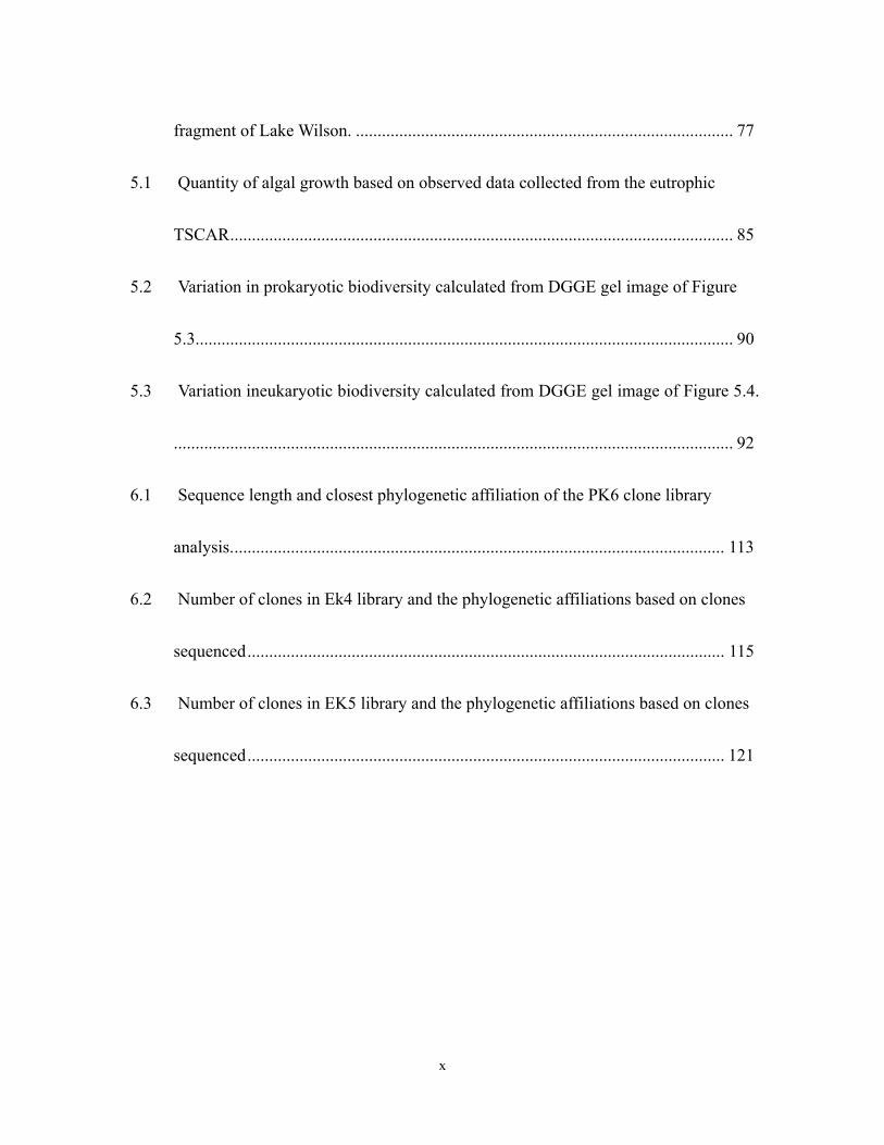
3.1 Experimental parameters of bioreactors based on Vollenweider model dividing the

three classified trophic states. ................................................................................. 24

3.2 The system of trophic-state-classified algal reactors (TSCARs) ........................... 26

3.3 Chl a concentaction (X) collected from TSCAR eutrophic bioreactor and relative

Chl a concentaction change ( tX ∆∆ ) and nr which used in the algal

bioproductivity calculation procedure. ................................................................... 33

3.4 Demonstration for algal areal product ( TP , mg/m2) based on )(tPr by using a set

of )(tPr functions (3.8)....................................................................................... 35

3.5 Cumulative TP (mg Chl a /m2) in the bioreactor over the time period. .............. 37

3.6 Flow diagram of the application of DGGE and molecular cloning to lake ........... 38

3.8 The plot of observed data by using step tracer input for the three bioreactors:

oligotrophic bioreactor, mesotrophic bioreactor, and eutrophic bioreactor, in

response to a continuous input. ............................................................................... 49

3.9 Algae growth patterns observed in three TSCAR bioreactors............................... 51

4.1 Kinetics of SRP in TSCARs. ................................................................................. 55

4.2 Observed data of TP concentration in TSCARs. ................................................... 59

4.3 Chl a concentration observed in TSCARs from Day1 to Day19........................... 60

xii

4.4 Cumulative TP (mg as Chl a /m2) in the bioreactor over the time period............... 61

4.5 Negative image of DGGE gel of 18/16S rDNA fragment for determining the

biodiversity. Image (a): DGGE analysis of 18S rDNA fragment. Image (b): DGGE

analysis of 16S rDNA fragment. Wahiawa reservoir sample collected on 26 Nov.

2008. lane1, lane2, and lane3 showed the DGGE band of 18S rDNA fragment

collected from oligotrophic, mesotrophic, and eutrophic bioreactor which samples

collected on Day12. lane4, lane5, lane6 showed DGGE band of of 16S rDNA

fragmen from oligotrophic, mesotrophic, and eutrophic bioreactor collected on

Day12...................................................................................................................... 66

4.6 Map of Lake Wilson watershed and sampling locations. 1: Downstream of Sewage

Treatment Plant (DSTP); 2: Wahiawa State Freshwater Park (WSFP). ................. 70

4.7 Vertical profile of DO and temperature at two sites of Lake Wilson..................... 73

4.8 DGGE analysis of 18/16S rDNA fragment for determining the biodiversity in Lake

Wilson by using DGGE banding pattern. Image (a): DGGE analysis of 18S rDNA

fragment. Image (b): DGGE analysis of 16S rDNA fragment. Lane1 and Lane3

represented the samples collected from DSTP of Lake Wilson; Lane2 and lane4

represented the samples collected from WSFP of Lake Wilson. ............................ 76

5.1 Observed data showed the algal X against time, t. Observed data of algal

xiii

populations size represented Chl a in eutrophic bioreactor. On Sep. 23 2011, 1.5

liter of lake water from Lake Wilson was introduced into eutrophic TSCAR

bioreactor described Chapter 3. The biomass by Chl a were collected daily until

2011, Oct. 4. ............................................................................................................ 84

5.2 Time-varying curve of algal net growth rate ( sr ) calculate from the observed data

of Figure 5.1. Phases of growth are defined as: phase I: positive algal net growth

rate (+ sr ) in act of increasing; phase II: positive algal net growth rate (+ sr ) in act

of decreasing; phase III: negative algal net growth rate (- sr ) in act of decreasing;

phase IV: negative algal net growth rate (- sr ) in act of increasing....................... 87

5.3 Negative image of DGGE gel of 16S rDNA fragment for determining the

prokaryotic biodiversity in TSCARs by using DGGE banding data. Nine bands are

interested which marked a, b, c, d, e, f, g, h and i................................................... 91

5.4 Negative image of DGGE gel of 18S rDNA fragment for determining the

eukaryotic biodiversity in TSCARs by using DGGE banding data. Five bands are

interested which marked E1, E2, E3, E4 and E5 on Day 12................................... 94

5.5 Phased relationships of prokaryotic biodiversity and algal specific net growth rate.

The open circle, open triangle and solid circle denote phase I (Day 1 to Day 6),

phase II (Day 7 to Day 9) and phase III (Day 10 to Day 12), representatively. ..... 97

xiv

5.6 The change of prokaryotic biodiversity resulted from algal bioproductivity based

on observational study. Open circle is the sampling day. The values of Pr are

calculated using the observed date of Figure 5.1.................................................... 98

5.7 Phased relationships of eukaryotic biodiversity and specific algal net growth rate.

The open circle, open triangle and solid circle denote phase I (Day 1 to Day6),

Phase II (Day7 to Day 9) and Phase III (Day10 to Day 12). ................................ 100

5.8 The act of changing eukaryotic biodiversity resulted from algal bioproductivity

based on observational study. Open circle is the sampled day. The values of Pr are

calculated using the observed date of Figure 5.1 referred to the procedure of Pr

estimation in Chapter 3. ........................................................................................ 101

5.9 Algal population growth showing the relation between the algal net growth rate

and algal population size X (Chl a). K is carrying capacity.................................. 103

5.10 Experiment results conducted at eutrophic TSCAR during Sept. 13, 2010 to Sept.

29 2010.................................................................................................................. 104

6.1 DGGE profile image of prokaryotic and eukaryotic cloning libraries termed Pk6,

Ek4, Ek5, and Ek6 with representative clones. (a) Comparison of DGGE profile of

the eutrophic bioreactor mixed community to prokaryotic clones containing insert

16S rDNA gene. Lane1, eutrophic bioreactor mixed community; Lane2, EP 3;

xv

Lane3, EP 5; Lane4, EP 13; Lane5, EP 15; Lane6, EP 16; Lane7, EP 18; Lane8, EP

19; Lane9, EP 29; Lane10, EP 30; Lane11, EP 61; Lane12, EP 62. (b) DGGE image

demonstrates that the DGGE banding data depicted the OTUs of each eukaryotic

libraries (lane1 :Ek4, lane2 :Ek5, and lane3: Ek6) ............................................... 108

6.2 The plots demonstrate that the relationship between number of OTUs and number

of individual in three trophic-level assemblages. ..................................................111

6.3 Relative abundance of clones represented in the nine phylogenetic groups in EK4

library. ................................................................................................................... 116

6.4 Relative abundance of clones represented in the 9 phylogenetic groups in EK5

library. ................................................................................................................... 123

6.5 Relative abundance of clones represented in the 9 phylogenetic groups in EK6

library. ................................................................................................................... 128

A.1 Digital banding data of DGGE gel........................................................................... 140

xvi

LIST OF ABBREVIATIONS

AB: Algal Bioproductivity

BASINS: Better Assessment Science Integrating point & Non-point Sources

BBM: Bold’s Basal Medium

BLAST: Basic Local Alignment Search Tool

CBD: Convention on Biological Diversity

Chl a: Chlorophyll a

CSTR: Completely Stirred Tank Reactor

CTAB: Cetyl Trimethyl Ammonium Bromide

DEM: Digital Elevation Model

DGGE: Denaturing Gradient Gel Electrophoresis

DNA: Deoxyribonucleic Acid

DO: Dissolved Oxygen

DSTP: Downstream of Sewage Treatment Plant

Ek4: Molecular Cloning Library of Eukaryote in Oligotrophic TSCAR

Ek5: Molecular Cloning Library of Eukaryote in Mesotrophic TSCAR

Ek6: Molecular Cloning Library of Eukaryote in Eutrophic TSCAR

EVM: Extreme Value Method

xvii

GIS: Geographic Information System

IC: Inorganic Carbon

LB: Lake Biodiversity

NFKS: North Fork Koukonahua Station

NMDS: Nonmetric Multidimensional Scaling

PCR: Polymerase Chain Reaction

Pk6: Molecular Cloning Library of Prokaryote in Eutrophic TSCAR

PLOAD: Pollutant Load Model

SFKS1: South Fork Koukonahua Station 1



SRP: Soluble Reactive Phosphorus

TC: Total Carbon

TDS: Total Dissolved Solids

TE buffer: Tris-Cl, EDTA Buffer

T-RFLP: Terminal Restriction Fragment Length Polymorphisms

TMDLs: Total Maximum Daily Loads

TN: Total Nitrogen

xviii

TOC: Total Organic Carbon

TP: Total Phosphorus

TSCARs: Trophic State-Classified Algal Reactors

TSI: Carlson Trophic State Index

TSS: Total Suspended Solids

USEPA: US Environmental Protection Agency

WSFP: Wahiawa State Freshwater Park

WWTP: Wahiawa Wastewater Treatment Plant

xix

LIST OF SYMBOLS

LA = Area over a photoperiod, [L2]

sA = Area of reservoir surface, [L2]

AU = Area of land use type u, [L2]

C=Output concentration of tracer, [ML-3]

C0 =Input concentration of tracer, [ML-3]

gC =Constant determined by grazing effect, [none]

CU =Event mean concentration for land use type u, [ML-3]

D=Dilution rate, [T-1]

E =Evenness, [none]

H =Mean depth of lake water, [L]

H’=Shannon index, [none]

K=Carrying Capacity, [ML-3]

Kb=Exponential constant, [none]

LP=Pollutant load, [MT-1]

jN =Total peck height of intensity of j th lane, [none]

in =Intensity of peck height of i th band, [none]

P=Productivity, [ML-2T-1]

xx

PJ =Ratio of storms producing runoff, [none]

rP =Algal bioproductivity, [ML-2T-1]

rP =Average algal bioproductivity, [ML-2T-1]

TP =Areal algal product, [ML-2]

p =SRP concentration, [ML-3]

0p =Initial SRP concentration, [ML-3]

ijp =Importance probability of band at i pixel position on j lane, [none]

ssp = SRP concentration under steady-state, [ML-3]

Q =Flow, [L3T-1]

q =Hydraulic overflow rate, [LT-1]

R=Respiration, [ML-3T-1]

Rf =Precipitation, [LT-1]

RVU=Runoff coefficient for land use type u, [none]

gr =Specific algal growth rate, [T-1]

nr =A change in algal concentration during a unit time, [ML-3T-1]

sr =Algal net growth rate, [T-1]

S=Total band count on one lane, [none]

Sr=Species richness, [none]

xxi

T= Photoperiod, [T]

t =Time, [T]

Rt =Mean hydraulic resident time, [T]

V=Volume, [L3]

sv =Net settling velocity, [LT-1]

W’=Areal loading of TP, [ML-2T-1]

tW =Phosphorus loading from external sources, [MT-1]

X =Chl a concentration of algae, [ML-3]

iX =Input Chl a concentration, [ML-3]

λX =Concentration of the predator species populations, [ML-3]

z =Depth of the bioreactor, [L]

gµ =Algal gross growth rate, [T-1]

lλ =Algal net loss rate, [T-1]

θ = t/ Rt , [none]

pτ = Phosphorus resident time, [T]

σ = First-order loss coefficient, [T-1]

wρ = Flushing coefficient, [T-1]

φ = First-order total elimination coefficient, [T-1]

1

CHAPTER 1. INTRODUCTION

Eutrophication has been widely recognized as a primary water quality issue

affecting aquatic systems, particularly for most of lakes in the world (Asai, Ootani, et al.

2003; Vollenweider 1971; Zison, Mills, et al. 1978). Although eutrophication has often

been described as a natural aging process, most of the eutrophic process characterized by

the state results from nutrient enrichment and is accelerated by human activities. Many

undesirable side effects and economic issues have been raised regarding eutrophication

problems. These effects are associated with the excessive plants growth (e.g.

phytoplankton). Plankton plays a central role in man-made eutrophication problems. In

lakes, the health-related symptom of eutrophication is algal bloom. Algal bloom causes

bottom-water hypoxia, and the toxin product, resulting in fish death and health risk

mentioned in some cases (Conley, Paerl, et al. 2009; Hasler and Swenson 1967). Many

species of algae, including photosynthetic prokaryote and eukaryote, may produce toxic

compounds when algal bloom occurs in freshwater. This suggested that one of the most

significant relationships between phytoplankton growth and its dynamic composition

may provide the solution to eutrophication in lakes.

Although many researches emphasized the importance of eutrophication and the

2

water quality management strategy of controlling nutrient loading received from heavily

human-activated watersheds (Chou, Lee, et al. 2006; Schindler 1977; Schindler, Hecky,

et al. 2008), many key questions of the scientific fundamentals in eutrophication were far

from settled. Several attempts have been made on the scientific knowledge of

eutrophication processes by investigating the relationship between the biological activity

and variation of the plankton (Dodson 2000; Striebel, Behl, et al. 2009). Many documents

indicated that the nutrient-stimulated eutrophication process is able to alter the species

composition such as eukaryotic and prokaryotic community structure and its correlated

bioproductivity (Chauhan, Fortenberry, et al. 2009; Horner-Devine, Leibold, et al. 2003;

Yannarell, Kent, et al. 2003). For instance, Horner-Devine (2003) established microcosms

by controlling the input of inorganic nutrient to assess the relationship between primary

productivity and diversity. They found that algae and particular taxonomic groups of

bacteria richness varied with primary productivity.

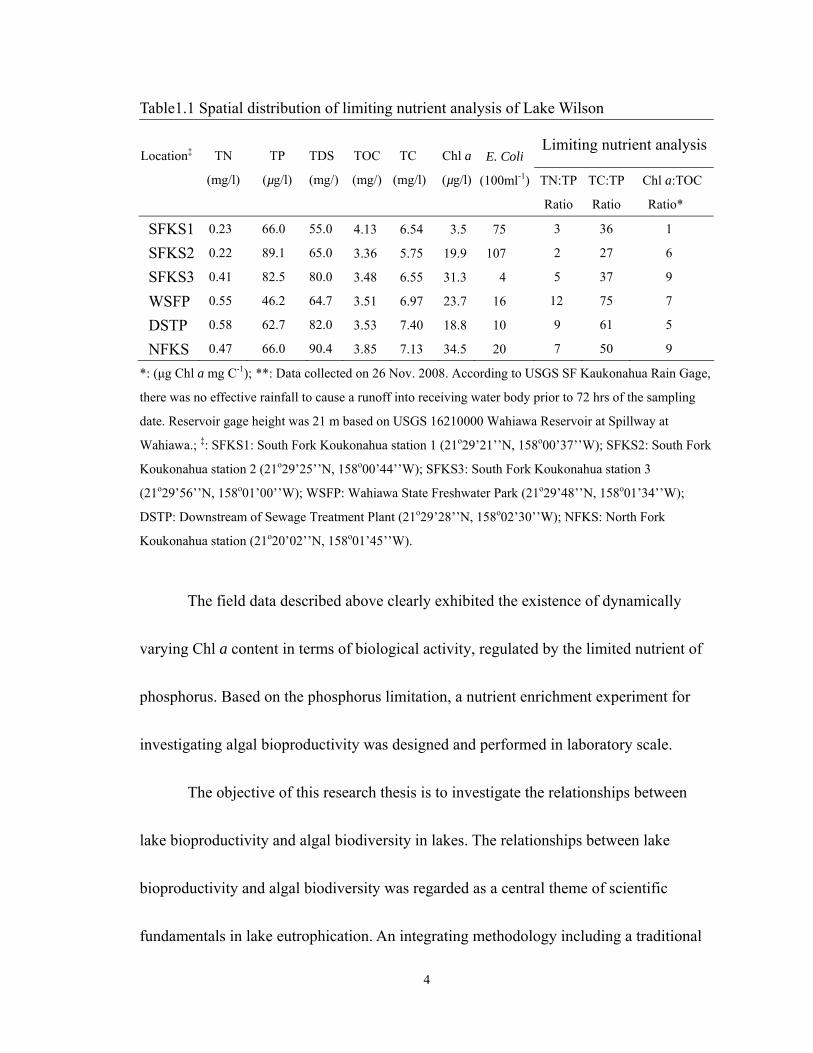
During 2008 to 2010, a general survey conducted showed the status of trophic

levels of Lake Wilson. The Chl a, total carbon, total phosphorus and total nitrogen were

monitored in the Lake Wilson. There were variations in Chl a concentrations in both

temporal and spatial trends. The wide range of Chl a concentration (means, ±standard

deviations) between 45.9 to 12.2 µg/L (mean=27.7, ±11.5, n=11) was monitored at WSFP

3

(Wahiawa State Freshwater Park) site. The data showed an average concentration of

410µg as N/L total nitrogen (±155, n=6), 69 µg as P/L total phosphorus (±15, n=6), and

3,077 µg as C/L inorganic carbon (±590, n=6). Based on the survey of 26 Nov. 2008,

there exhibited the spatial variations in ratio of N:P and ratio of C:P in the water as shown

in Table 1.1. The ratio of C:P was higher than 27 at all monitored locations. The ratio of

N:P was higher than 7.2 at two locations: 1) Wahiawa State Freshwater Park and, 2)

downstream of Wahiawa Wastewater Treatment Plant (WWTP). This observed data

(Table 1.1) released the information about the spatial scale difference of the limiting

nutrient. In general, the higher N:P ratio(e.g. >7.2) indicated that phosphorus was the

limited element regulating algal bioproductivity in lake water (Chapra 1997). In practice,

phosphorus control has succeeded in preventing eutrophication in many lakes (Schelske

2009; Schindler 1974). It is possible that the effluent contributed sufficient nitrogen

nutrient to the lake from the sewage treatment plant. This implies that phosphorus limited

the algae growth near the outfall of the sewage treatment plant due to the N:P ratio being

higher than 7.2, that is, phosphorus regulates the algal growth in two locations of Lake

Wilson.

4

Table1.1 Spatial distribution of limiting nutrient analysis of Lake Wilson

Limiting nutrient analysisLocation‡

TN

(mg/l)

TP

(µg/l)

TDS

(mg/)

TOC

(mg/)

TC

(mg/l)

Chl a

(µg/l)

E. Coli

(100ml-1)

TN:TP

Ratio

TC:TP

Ratio

Chl a:TOC

Ratio*

SFKS1 0.23 66.0 55.0 4.13 6.54 3.5 75 3 36 1

SFKS2 0.22 89.1 65.0 3.36 5.75 19.9 107 2 27 6

SFKS3 0.41 82.5 80.0 3.48 6.55 31.3 4 5 37 9

WSFP 0.55 46.2 64.7 3.51 6.97 23.7 16 12 75 7

DSTP 0.58 62.7 82.0 3.53 7.40 18.8 10 9 61 5

NFKS 0.47 66.0 90.4 3.85 7.13 34.5 20 7 50 9

*: (µg Chl a mg C-1); **: Data collected on 26 Nov. 2008. According to USGS SF Kaukonahua Rain Gage,

there was no effective rainfall to cause a runoff into receiving water body prior to 72 hrs of the sampling

date. Reservoir gage height was 21 m based on USGS 16210000 Wahiawa Reservoir at Spillway at

Wahiawa.; ‡: SFKS1: South Fork Koukonahua station 1 (21o29’21’’N, 158o00’37’’W); SFKS2: South Fork

Koukonahua station 2 (21o29’25’’N, 158o00’44’’W); SFKS3: South Fork Koukonahua station 3

(21o29’56’’N, 158o01’00’’W); WSFP: Wahiawa State Freshwater Park (21o29’48’’N, 158o01’34’’W);

DSTP: Downstream of Sewage Treatment Plant (21o29’28’’N, 158o02’30’’W); NFKS: North Fork

Koukonahua station (21o20’02’’N, 158o01’45’’W).

The field data described above clearly exhibited the existence of dynamically

varying Chl a content in terms of biological activity, regulated by the limited nutrient of

phosphorus. Based on the phosphorus limitation, a nutrient enrichment experiment for

investigating algal bioproductivity was designed and performed in laboratory scale.

The objective of this research thesis is to investigate the relationships between

lake bioproductivity and algal biodiversity in lakes. The relationships between lake

bioproductivity and algal biodiversity was regarded as a central theme of scientific

fundamentals in lake eutrophication. An integrating methodology including a traditional

5

assessment method and state-of-the-art molecular biotechnology was developed to assess

this problem.

Based on the objective, the algal bioproductivity and lake biodiversity were

investigated under the laboratory scale and a field study. The following tasks were

fulfilled: (i) to establish the laboratory-scale experiment for simulating eutrophication

process; (ii) to investigate the algal bioproductvity; (iii) to investigate the lake

biodiversity of eukaryotes and prokaryotes in lakes by varying the trophic levels under

stable state; (iv) to investigate lake biodiversity with time-varying algal bioproductivity;

(v) to determine the structure of eukaryotic assemblage under differing the trophic status.

To ensure that the relevant tasks are able to accomplish the objective, Chapter 2

provides a comprehensive literature review of the importance of eutrophication and algal

bloom in water resource management, the current knowledge of lake bioproductivity, the

introduction of current molecular biotechnology in examining the biodiversity and the

methods of identifying the eukaryotic structure among trophic levels. Chapter 2 reviews

the traditional and current treatments in study of the man-made eutrophication problems

and summarizes the critical control factors, limited nutrient such as the element of

phosphorus or nitrogen in lake systems. Chapter 3 portrayed the methodology used for

investigating the algal bioproductivity estimation and its lake biodiversity. A set of

6

methods contains the experimental concept, theorem of CSTR bioreactors, algal culture,

the principle of bioproductivity calculation and the protocols of examining biodiversity,

and illustrates the performance of bioreactors including the hydraulic behavior, algal

growth patterns and the related utilization of phosphorus.

Chapter 4 represents the relationships of biodiversity-bioproductivity based on the

bioreactors of the gradient trophic levels: oligotrophic, mesotrophic and eutrophic status.

And the relationships of biodiversity-bioproductivity also were paralleled with field study

in Lake Wilson. Chapter 5 illustrates how the lake biodiversity was regulated by

biological activity factor, algal bioproductivity during the varying algal growth phases

carried out in a eutrophic bioreactor. The observation was conducted by using

time-varying analysis which demonstrates the general correlation between eukaryotic and

prokaryotic biodiversity and its algal bioproductivity. Chapter 6 presents the composition

of the eukaryote community, differentiated by trophic levels. These trophic levels were

constructed out of three libraries: oligo, meso, and eutrophic libraries. Chapter 7 provides

the conclusion and perspective of these efforts.

7

CHAPTER 2. LITERATURE REVIEW

To ensure that the relevant tasks are able to accomplish the objective, chapter 2

provides a comprehensive literature review. This review includes the importance of

eutrophication and algal bloom in water resource management, the current knowledge of

algal bioproductivity, an introduction to advance modern molecular techniques in

examining the biodiversity, and identifies the eukaryotic structure among trophic levels.

Chapter 2 reviews the traditional and current treatments in studies of the artificial

eutrophication problems and summarizes the critical control factors, limited nutrients,

such as the elements of phosphorus or nitrogen in lake systems.

2.1 Lake eutrophication and algal bloom

Eutrophication is organized as a pollution problem in lakes and reservoirs since it

has a number of deleterious effects on aquatic systems (Bowie, Mill, et al. 1985; USEPA

1974). Many species of algae, including photosynthetic prokaryotes and eukaryotes, may

produce toxic compounds when algal bloom occurs in marine and freshwater. Some

reports have shown that these toxins have caused the fatal human poising and the death of

nonhuman mammals in New Zealand, Japan, Canada, the United States and Great Britain

(Ryoichi, Ootaini, et al. 2003). A number of eutrophication studies have primarily

8

focused on the development of the assessment method of using a single or multi index of

eutrophication (Carlson 1977; Kasprzak Padisák, et al. 2008). Carlson Trophic State

Index (TSI) has also been used to estimate the trophic state of reservoirs and lakes. Lakes

were often classified based on its trophic state (Carlson 1977; Chou, et al. 2006; USEPA

1974; Vollenweider 1968).

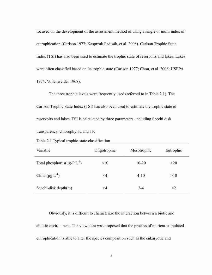
The three trophic levels were frequently used (referred to in Table 2.1). The

Carlson Trophic State Index (TSI) has also been used to estimate the trophic state of

reservoirs and lakes. TSI is calculated by three parameters, including Secchi disk

transparency, chlorophyll a and TP.

Table 2.1 Typical trophic-state classification

Variable Oligotrophic Mesotrophic Eutrophic

Total phosphorus(µg-P L-1) <10 10-20 >20

Chl a (µg L-1) <4 4-10 >10

Secchi-disk depth(m) >4 2-4 <2

Obviously, it is difficult to characterize the interaction between a biotic and

abiotic environment. The viewpoint was proposed that the process of nutrient-stimulated

eutrophication is able to alter the species composition such as the eukaryotic and

9

prokaryotic community structure, with its correlated bioproductivity (Horner-Devine, et

al. 2003). Over the years, the trophic state of upland reservoirs subject to man-made

pollution has been assessed by using the Vollenweider model (Vollenweider 1968) and/or

Carlson Trophic State Index (TSI)(Carlson 1977). The Vollenweider model was

formulated by assuming that the reservoir behaves as a completely stirred tank reactor

(CSTR) and that phosphorus is the only limiting nutrient. It can be expressed as the

following equation: QppAvWdtdpV sst −−= , where V is the water volume of the

reservoir; p is the concentration of TP; Q is the outflow; t is time; tW is the

phosphorus loading from external sources; sv is the net settling velocity; sA is the

reservoir surface area. US Environmental Protection Agency (USEPA 1974) suggested

that a reservoir is under an oligotrophic state while the average TP concentration is below

10 (µg L-1), and a reservoir is under an eutrophic state while the average TP concentration

is more than 20 (µg L-1). At a steady state, a Vollenweider model can be solved to yield

relationships between average annual TP loading (W’) and reservoir hydraulic properties

represented by H/ Rt , where H is the mean water depth and Rt = (H As)/Q is the mean

hydraulic residence time.

Limited nutrient and algal growth

Monod model and Droop model are well-known kinetics models that express the

10

relationship between nutrient uptake and algal growth. The Monod model described that

the algal growth is governed by external nutrients. The Droop model stated that the algal

growth kinetics is a function of internal nutrient such as phosphorus or vitamin (Droop

1974). In previously study, TP concentrations of lakes were investigated by Hudson and

Taylor (2000) from 56 lakes in North America (Hudson, Taylor, et al. 2000). This

research pointed out that the soluble reactive phosphorus (SRP) was often under

picomolar concentration in lakes which along different trophic statuses. The SRP was

increased along the ascent of trophic levels. Similar results were detected in TSCAR

experiments. The result of laboratory experiments showed that the SRP concentrations of

three trophic levels are 1.5~4.5, 2.5~6, and 8~20 :g/L for oligo, meso and eutrophic

bioreactors, respectively. The SRP is the biologically availability nutrient for maintaining

the primary productivity in lake. In general, the loading from runoff is recognized as the

major source of nutrient in lake. Recently, the study showed that the available phosphorus

for lake plankton growth obtained from internal source such as the plankton community,

rather than from external loading (Hudson, Taylor, et al. 1999).

11

Table 2.2 SRP and TP in lakes and laboratory experiments Lake/reactor SRP(:g/L) TP(:g/L) Trophic level Reference Flathead Lake 0.4~0.5 2.4~4.6 oligotrophic Graig N. Spencer

and Bonnie K. Ellis 1998; Hudson, et al. 2000.

Jacks Lake

--- 15.5 mesotrophic Hudson, et al. 2000

Halfmoon Lake

--- 80.6 eutrophic Hudson, et al. 2000

Wahiawa Reservoir (Wahiawa State

Freshwater Park)

8.7~12.7 26.5~46.0 eutrophic This research

Oligotrophic bioreactror

1.5~4.0 3.30 oligotrophic This research

Mesotrophic bioreactor

2.0~4.5 16.50 mesotrophic This research

Eutrophic bioreactor

2.5~10.0 34.65 eutrophic This research

The relationships between the total phosphorus and TN, Chl a, and total carbon

have a positive linear relationship based on the study by Schindler (Schindler 1977). In

order to control eutrophication in lake, we have to figure out which is the critical element

of nutrients such as nitrogen (N) and phosphorus (P). Schindler et. al. (Schindler, et al.

2008) indicated that eutrophication in a lake can not be controlled by reducing the input

total loading of nitrogen. They concluded that eutrophication management must be more

concerned about the problem on the input loading of phosphorus from watershed. The

12

phosphorus loading from watersheds include a point source and a non point source. In

this research we used PLOAD/BASINS (Pollutant Load/Better Assessment Science

Integrating point & Non-point Sources) to estimate the phosphorus loading from

watershed shown as Table 2.3.

Table 2.3 Phosphorus loading of Lake Wilson estimation

Inflow Loading(tn/yr) Estimated method Non point source: Watershed runoff

3.1 PLOAD/ BASINS

Point source: Wahiawa wastewater treatment plant effluent

3.5 Data provided from WWTP

Algal growth kinetics is described based on three principle components:

temperature effect, solar radiation, and nutrient effect. The first order reaction model and

Michaelis-Menten model are the most common approaches to illustrate the algal growth

kinetics. Laws and Chalup (1990) developed an approach of chlorophyll content basis

that attended to integrate the effect of light and nutrient level in algal growth kinetics

(Laws and Chalup 1990). In this approach, the behavior of algal growth kinetics such as

growth rate and respiration rate is stimulated.

The half saturation rate of Michaelis-Menten model represents the affinity of the

alge for the nutrient throughout transporter and receptor of cell wall to uptake or transport

13

nutrient from external water. A study shown that phosphate uptake rate in each species

examined was a function of external phosphorus, substrate concentration and intracellular

phosphorus level (Ivan and Rhee 1981). On the other hand, it was known that the

metabolism of organic carbon within cells varies related based on phosphate uptake. TP

concentration is often used to classify trophic status as mentioned above. However, it was

known that phytoplankton’s nutrient growth limitation is a function of its internal

concentration rather than the nutrient concentration in water.

2.2 Algal bioproductivity

In common usage, the term “bioproductivity” is often used to expound the

product of photosynthesis. For example, the book, Technique in Bioproductivity and

Photosynthesis, edited by Coombs et. al. (1985) provides the introduction to

methodologies for investigation of photosynthetic limitations to bioproductivity in natural

and artificial systems (Coombs 1985). Bioproductivity was often used to describe the

biomass yields of algae in field and bioreactors (Gordon and Polle 2007; Janssen,

Tramper, et al. 2003). In this research, however, the bioproductivity can be considered as

the increasing content of biomass per unit area and per unit time (e.g. mg m-2 day-1)

through the process of photosynthesis, and results in the conversion of light energy to

chemical energy. Biomass can be expressed as conserved quantity, e.g. weight of Chl a,

14

organic matter, carbon, or energy. The bioproductivity can be measured by the variation

of the amount of 14C (Yoo 2008), Chl a (Chapra 1997), dry weight (Gordon and Polle

2007) or dissolved oxygen (Odum 1956) per unit of time.

Carbon- based estimation

Compared with alternative methods, the 14C method represents the carbon fixed

that it is a direct technique to measure algal bioproductivity. The estimate of

bioproductivity is fundamentally different than productivity measured in other

ecosystems (e.g., grasslands, forests). With the advanced measure technology, the

easy-to-measure content (e.g. Chl a and DO) was utilized as an alternative in contrast to

the direct measure (14C method). On the basis of literature, the range of algal

bioproductivity is approximately 525~20,805g C/m2/yr in eutrophic lakes (Gelin 1975)

and 1~54.75 g C/m2/yr in oligotrophic lakes (Waide, Willig, et al. 1999). Under lower

temperature lakes, 11.3g C/m2/yr in eutrophic lake and 4.1g C/m2/yr in oligotrophic lake

were observed (Kalff and Welch 1974).

Chlorophyll- based estimation

Kasprzak (2008) developed the Chlorophyll- based indicator which is able to

describe the broad trophic gradient of lakes (Kasprzak, et al. 2008). Laws and Chalup

(1990) developed an approach of chlorophyll content basis that attempts to integrate the

15

effect of light and nutrient level in algal growth kinetics (Laws and Chalup 1990). In this

approach, the behavior of algal growth kinetics such as growth rate and respiration rate is

stimulated.

The algal bioproductivity often is expressed as either the content of chlorophyll a

(Chl a) (Ryther and Yentsch 1957) or by the rate of production (Schallenberg and Burns

1997). Some research showed that high Chl a is not guaranteed to reflect high

bioproductivity because it can be merely the result of accumulation of Chl a. Therefore, it

is necessary that algal bioproductivity should be defined as a rate term and be the amount

of carbon fixed in unit area per unit time through photosynthesis. Kalff (1974) reported

that based on the plot of observed Chl a indicated around 1~6 mg Chl a /m2 in

oligotractic Char Lake and around 2~40 mg Chl a /m2 in eutrophic Meretta Lake (Kalff

and Welch 1974).

DO- based estimation

Bioproductivity can be represented as the content of dissolved oxygen (DO) in an

aquatic system. In the field study, the changes of diurnal DO can be observed, and then

we can interpret its significance in the lake’s water quality. In 1956, Odum pioneered in

the curve of diurnal dissolve oxygen (DO). Odum used the diurnal changes of dissolved

oxygen (DO) to calculate the component rate of bioproductivity and respiration. The

16

method was summarized as a procedure by Seeley (Seeley 1969). Odum (1956) also used

the curve of diurnal DO to evaluate the productivity and respiration. He indicated that the

ratio of the productivity and respiration can be used classify the freshwater communities

into autotrophic and heterotrophic types.

The oxygen-oriented water quality factor is considerably influenced by

photosynthesis, and respiration in particular, at the biological activity waterbody.

Photosynthesis is the process which tranforms sunlight energyby green plants as chemical

energy. It is also the most important biochemical pathway in aquatic ecosystem.

2612648photone

22 6OOHC6COO6H +⎯⎯⎯ →⎯+ (2.1)

Diurnal DO variation has been recognized as an indicator related to

phytoplankton and other aquatic green plants in a stream or reservoir (Odum 1956).

Wang et al. (2003) used an extreme value method (EVM) which employed the maximum

and minimum dissolved oxygen deficits affected by photosynthesis and respiration, to

estimate metabolism rates in streams (Wang, Hondzo, et al. 2003). This method

suggested that photosynthetic production could be estimated combining a mass balance

model with diurnal oxygen measurements.

2.3 Lake biodiversity

An operational definition and an appropriate measuring approach are important in

17

lake biodiversity (LB) research. The term "biodiversity," also called biological diversity,

was defined as the number of species in a given habitat (Encyclopedia 2009). The

concept of biodiversity also implies the variation of number in respect to species and

individual within the boundaries of a given space and time. Purvis (2000) explicated

“biodiversity is the sum total of all biotic variation from the level of genes to ecosystems”

(Purvis and Hector 2000). The hierarchical character of biodiversity showed the variety

under higher and lower level. Norse et al. (1986) established a hierarchy of biological

diversity at three levels: genetic diversity (within-species diversity), species diversity

(number of species), and ecological diversity (diversity of communities) (Harper and

Hawksworth 1994). To date, the study of biodiversity often investigates the three

biodiversity levels which are of within species, between species and of ecosystems. The

definition of three levels was expressed by the CBD (Convention on Biological

Diversity). This definition of CBD: “Biological diversity” means the variability among

living organisms from all sources including, inter alia, terrestrial, marine and other

aquatic systems and the ecological complexes of which they are part; this includes

diversity within species, between species and of ecosystem” was widely cited.

(https://www.cbd.int/ibd/2008/Resources/teachers/glossary.shtml). Some researcher have

begun to investigate the interaction and linking on these levels of diversity (Magurran

18

2005, Vellend 2005). Lake biodiversity is the variety of eukaryote and/or prokaryote in

defined space and a time of study. The definition of lake biodiversity which is used in

studying lake eutrophication is: “The variation of the richness and evenness among

eukaryotc and prokaryotic species in lakes.”

The measurement of biodiversity is well documented including theoretical and

practical guides (Magurran 1988). Much of what is known about the models and indices

was developed for addressing the temporal and spatial variation of biodiversity (Dunbar,

Barns, et al. 2002). The application of models often confronted considerable debate due

to the aspects of sampling (Gotelli and Colwell 2001; Magurran 1988), count technique

(Caron, Countway, et al. 2004), and species determination (Templeton 1994). These

problems of quantifying biodiversity were tackled by devising the indices and model

(Purvis and Hector 2000). The census of individual species play important role for fitting

the theoretical biodiversity models. For investigation of biodiversity, it is important for

the survey of the number of species and the proportional abundance of species. The

methods of surveys often depend on the level of biodiversity (Gaines, Harrod, et al. 1999).

The survey techniques include remote sensing and geographic information system (GIS)

for large-scale (Gaines, et al. 1999), D-net sweeps (Chase and Leibold 2002) for

macroorganisms, and staining, pigment analysis, transmission electron microscopy

19

(Caron, et al. 2004; Guillou, Chre´tiennot-Dinet, et al. 1999) and DNA fingerprinting

analysis (Templeton 1994) for picoplankton. The protocol of identification of the

eukaryote and prokaryote usually is that they are isolated and extracted by specific

culture media (e.g. sugar or agar) from their environment and then counted and identified

by microscope or in hand. The limitation of studying lake biodiversity by using an optical

instrument is that it can not promise to count the totality of species, due to little species

that can be cultured on medium due to the tiny size and lack of distinctive taxonomic

characters (Moon-van der Staay, De Wachter, et al. 2001). The biodiversity assessment

by a DNA-based approach provides the a huge amount of invaluable species information

(Caron, Countway, et al. 2009; Magurran 2005; Vellend 2005). Molecular approaches

provide many advantages for biodiversity assessment. These approaches can be used to:

identify the species according to the data of DNA sequences to know what species are the

dominant; distinguish the species and subspecies to exhibit the phylogenetic position; and

quantify the relative amount of species (Caron, et al. 2004; Karp, Edwards, et al. 1997).

The molecular biotechnology (e.g. denaturing gradient gel electrophoresis, molecular

cloning, sequence, and fragment analysis) can detect the variation in DNA level (Karp, et

al. 1997).

In the past, numerous studies tried to use molecular biotechnology to explore a

20

more effective method to detect and diagnose the ecosystem. Nowadays, molecular

signals have been used to distinguish organisms and represent their responses for the

effects of a physical and chemical environment. The use of molecular signals as an

assessment indicator for water quality comes with a few advantages which provide an

early warning of possible environmental deterioration and sensitive measures of pollutant.

A molecular tool is now in widespread used because it provides more detailed

information on genetic content. This information from a specific gene sequence (e.g.18S

rDNA) provides the basis for identification and quantification of eukaryotic micrograms.

Ryoichi et al. (2003) developed a technique, PCR-based ribosomal DNA detection

technique, to detect the bloom-forming genus of algae (Ryoichi, et al. 2003). The small

subunit ribosomal DNA gene (e.g. 16S rDNA) sequence is used for analyzing

phylogenetic relationships among the diversity taxa because it presents the properties of

both highly conserved and variable region.

These are a number of approaches used to investigate genetic diversity. These

approaches include denaturing gradient gel electrophoresis (DGGE), and terminal

restriction fragment length polymorphisms (T-RFLP) based on the DNA fragment length

(Caron, et al. 2004). Muyzer G. et al.(1993) demonstrated an approach where they used

DGGE to separate the specific gene sequence, 16S rDNA, obtained after PCR

21

(Polymerase Chain Reaction) amplification of genomic DNA extracted from microbial

community population (Muyzer, Ellen, et al. 1993). Van Hannen et.al (1999) documented

that nonmetric multidimensional scaling (NMDS) using statistical analysis to calculate

the distance matrix converted from DGGE banding patterns provides a bidimensional

plot to compare the migration of bacteria and eukaryotic community occurred after the

change of condition (Van Hannen, Mooij, et al. 1999). Carrino-Kyker (2008) interpreted

the importance of abiotic condition influence on the macroorganisms (Carrino-Kyker and

Swanson 2008). They also used NMDS to analyze the temporal and spatial patterns of

eukaryotic and bacterial communities. Muyzer (1998) presented the method of DGGE

which is employed to construct the information of biodiversity on marine or freshwater

(Muyzer and Kornelia 1998). They emphasized the significance of molecular biological

technique particularly on detecting and identifying microorgams. The molecular marker

(16S rDNA) or encoding gene is used to investigate the microbial diversity and analyses

their structure of microbial communities.

In this study, DGGE technique shows an advantage that it has the ability of an

immediate display of the population composition with less time-consuming and laborious.

Lefranc M. et al. (2005) performed a study that they selected oligotrophic, mesotrophic,

and eutrophic lakes and then used molecular biotechnology to analyze the diversity of

22

small eukaryotes. The study showed that the population composition of eukaryotes varied

with the trophic levels (Lefranc, Thenot, et al. 2005).

The relationships between algal bioproductivity and lake biodiversity commonly

are expressed concisely as four patterns (mono hump-shaped, U-shaped, positive, and

negative) (Chase and Leibold 2002; Drake, Cleland, et al. 2008). The patterns were

observed and concluded that highly related to the size of spatial scale (Chase and Leibold

2002), the level of nutrition (Lefranc, Thenot et al. 2005), the amount of available energy

and the extent of invasion of non-native species (Chase and Leibold 2002).

Lake biodiversity (AB) is defined as the variety of eukaryotes and prokaryotes in

the defined space and time of study. To investigate algal biodiversity, the method must be

able to distinguish, identify and enumerate individual species. For this purpose,

microscopic observation has been employed to study ecological diversity (Chase and

Leibold 2002; Chien, Wu, et al. 2009; Gaines, et al. 1999). Yet the limitations of

morphology and other classical taxonomic characters have been recognized for the use of

the method of microscopic observation to study biodiversity (Caron, et al. 2004;

Hammond 1994). The molecular observation methods probing specific genes (e.g. 16S r

DNA and 18S rDNA) encoding particular species are useful tools to investigate

biodiversity (Caron, et al. 2009; Karp, et al. 1997; Magurran 2005; Vellend 2005).

23

CHAPTER 3. METHODOLOGY

Chapter 3 represents the methodology used for investigating the algal

bioproductivity and its related lake biodiversity in lakes. A set of methods contains

experimental design, the use of CSTR bioreactors, algal culturing techniques, the

estimates of bioproductivity and the protocols of examining biodiversity, and illustrates

the performance of three trophic state-classified algal reactors (TSCARs) including the

hydraulic behavior, algal growth patterns and the related utilization of phosphorus.

3.1 Experimental design

To study algal bioproductivity, the system of trophic state-classified algal reactors

(TSCARs) was constructed and operated in the laboratory. The TSCARs provided a

lake-like microcosm to perform a simulation of a gradient trophic state for lakes which

promoted the algae growth. The design and operation parameters of the TSCARs system

are summarized in Table3.1. The determination of hydraulic overflow rate (q) and areal

loading of TP (W’) is based on the Vollenweider model (Vollenweider 1976). According

to the theorem of mass balance, under steady state this W’ and q can be solved

for )10(01.0' += qW and )10(02.0' += qW (Dillon 1975). Vollenweider (1976)

suggested that the mesotrophc state may be restricted by TP concentration within 10 and

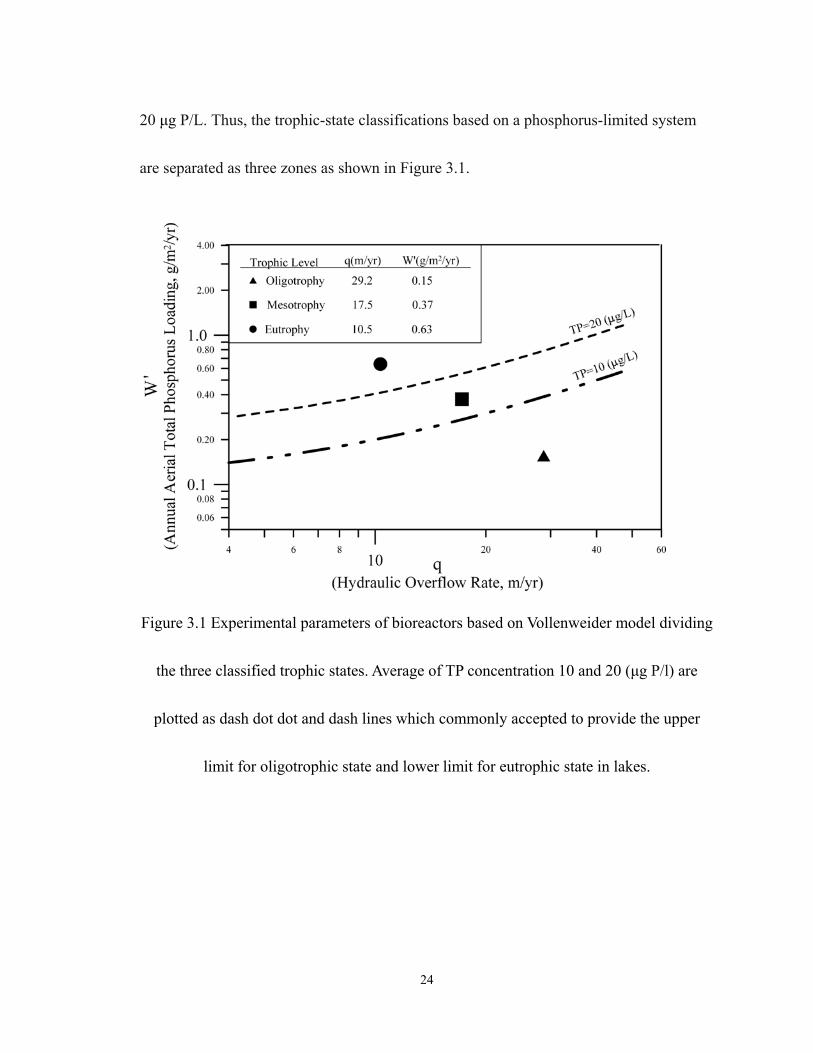
24

20 µg P/L. Thus, the trophic-state classifications based on a phosphorus-limited system

are separated as three zones as shown in Figure 3.1.

Figure 3.1 Experimental parameters of bioreactors based on Vollenweider model dividing

the three classified trophic states. Average of TP concentration 10 and 20 (µg P/l) are

plotted as dash dot dot and dash lines which commonly accepted to provide the upper

limit for oligotrophic state and lower limit for eutrophic state in lakes.

25

Table 3.1 Experimental parameters of TSCARs based on the Vollenweider plot dividing the three categories of trophic levels

Design parameters Operation parmeters

Bioreactor Hydraulic overflow

rate (q, m/yr)

Areal loading of TP

(W’, g/m2/yr)

Flow rate

(ml/min)

TP concentration

(µg P/L) Oligotrophic 29.2 0.15 2.6 5 Mesotrophic 17.5 0.37 1.5 15 Eutrophic 10.5 0.63 0.9 60

The reactor of TSCARs was a rectangular tank with a total volumetric capacity of

0.015 m3 and a surface area of 0.045 m2. A metal-halide light source (GE Muli-Vapor

Lamp) was selected for the experiments to provide desirable light intensity ranges. A

sterile growth medium at varying nutrient concentrations and flow rates was fed through

bioreactors. The test apparatus utilized diffused-air agitation to simulate completely

stirred tank reactors. The air diffuser was installed on the bottom of the culture vessel to

facilitate air-bubble agitation throughout the culture vessel. The diffused air also supplied

dissolved CO2 for algal growth.

26

Figure 3.2 The system of trophic state-classified algal reactors (TSCARs)

TP was used as the limiting nutrient controlling different trophic states within the

test apparatus. Determination of hydraulic overflow rate (q) and areal loading of total

phosphorus (W’) were based on the Vollenweider model (Vollenweider 1971). Bold’s

basal medium (BBM) (Bold 1949) was adopted for algae cultivation to create the

limited-nutrient condition of phosphorus. TP were 5 µg P/l, 15 µg P/l, and 60 µg P/l of

K2HPO4. BBM contains the mixture with the final concentration, 2.94 mM NaNO3, 0.17

mM CaCl2 2 H2O, 0.304 mM MgSO4 7H2O, 0.428 mM NaCl, EDTA, Acidified Iron,

FeSO4 7H2O, 0.185 mM H3BO3, 30.7µM ZnSO4 7H2O, 7.28µM MnCl2 4 H2O, 4.93µM

MoO3, 6.29µM CuSO4 5H2O, 1.68µM CoCl2 6H2O and 5µM, 15µM, and 60µM K2HPO4

(KH2PO4) for forming the three trophic states. The modified BBMs were autoclave

27

sterilized at 121°C for 20 min before use. The test apparatus was continuously irradiated

at 8900 W/m2 with metal-halide lamp (400 Watt, GE Multi-Vapor Lamp). The

photoperiod was 24 hours during whole period of cultivation. The inoculums of algae

were introduced from the Lake Wilson sample and added to the three bioreactors using a

ratio (1:10) of inoculum to BBM.

Parameters including algae cell numbers, Chl a, pH, TN, TOC, TP, SRP, TSS, and

turbidity were monitored during the field investigation and laboratory experiments. The

quantification of Chl a was achieved by adsorption measurements using three different

wave lengths (664, 647, and 630 nm) by a spectrophotometer (DR/4000, HACH). Direct

microscopy counting of algae cell numbers was accomplished using a hemocytometer

(Hausser Scientific, Horsham, PA) and a bright-field microscope. TP and SRP were

determined by using a PhosVer 3 kit and a DR/4000 Hach spectrophotometer following

the procedure provided by the manufacturer. TN was measured using a TOC-VCPN

instrument (Shimadzu Corporation, Kyoto, Japan) based on the oxidative

combustion-chemiluminescence mechanism. Water-sample turbidity was measured using

a Model 2100N Laboratory Turbidimeter with a working range of 0 to 4000

Nephelometric Turbidity Units. Total carbon (TC), inorganic carbon (IC), and TOC in

water samples were measured using a TOC-VCPH/CPN instrument (Shimadzu

28

Corporation, Kyoto, Japan). Total suspended solids was determined based on the

Standard Method 2540 D (Eaton, Clesceri, et al. 2005). Total dissolved solids (TDS) of

water samples were determined using Standard Method 2540C (Eaton, et al. 2005). An

Orion® 720A+ Dual Channel pH/ISE Meter (Thermo, Waltham, MA) was used for pH

measurements. YSI 58 DO meter and YSI 600R DO Sonde (YSI, Inc., Yellow Springs,

Ohio) were used for DO measurements.

3.2 Estimates of algal bioproductivity

The estimates of algal bioproductivity are based on the changes in algal biomass

in terms of Chl a content which occurs in a given aquatic system during a unit of time. In

the equation (3.1), the mass balance model represents the changes of Chl a in the given

system during a unit time. Changes in Chl a content resulted from the algal growth and

loss processes can be represented by algal net growth rate ( sr ) consisting of the algal

gross growth rate ( gµ ) and algal net loss rate ( lλ ). In the equation (3.2a), the first term

expresses the gross growth rate ( gµ ), and the second term represents the net loss rate

( lλ ). The net loss rate combined with respiration rate, settling rate, decomposition rate

and grazing rate is modeled by assuming which loss rate is directly proportional to the

algal biomass.

The algal bioproductivity could be simulated by the mass balance model in

29

conjunction with the changes of Chl a concentration. Based on the mass balance equation,

the algal bioproductivity model for a well-mixed lake can be written as:

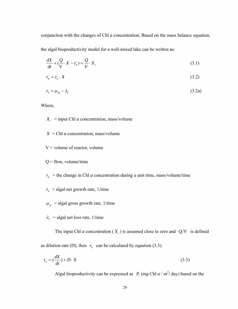
in XVQrX

VQ

dtdX

⋅=−⋅+ )( (3.1)

Xrr sn ⋅= (3.2)

lgsr λµ −= (3.2a)

Where,

iX = input Chl a concentration, mass/volume

X = Chl a concentration, mass/volume

V = volume of reactor, volume

Q = flow, volume/time

nr = the change in Chl a concentration during a unit time, mass/volume/time

sr = algal net growth rate, 1/time

gµ = algal gross growth rate, 1/time

lλ = algal net loss rate, 1/time

The input Chl a concentration ( iX ) is assumed close to zero and VQ is defined

as dilution rate (D), then nr can be calculated by equation (3.3).

XDdtdXrn ⋅+= )( (3.3)

Algal bioproductivity can be expressed as rP (mg Chl a / m2/ day) based on the

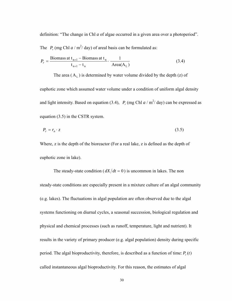
30

definition: “The change in Chl a of algae occurred in a given area over a photoperiod”.

The rP (mg Chl a / m2/ day) of areal basis can be formulated as:

)Area(A 1

ttat t Biomassat t Biomass

Ln1n

n1n ⋅−−

=+

+rP (3.4)

The area ( LA ) is determined by water volume divided by the depth (z) of

euphotic zone which assumed water volume under a condition of uniform algal density

and light intensity. Based on equation (3.4), rP (mg Chl a / m2/ day) can be expressed as

equation (3.5) in the CSTR system.

zrP nr ⋅= (3.5)

Where, z is the depth of the bioreactor (For a real lake, z is defined as the depth of

euphotic zone in lake).

The steady-state condition ( 0=dtdX ) is uncommon in lakes. The non

steady-state conditions are especially present in a mixture culture of an algal community

(e.g. lakes). The fluctuations in algal population are often observed due to the algal

systems functioning on diurnal cycles, a seasonal succession, biological regulation and

physical and chemical processes (such as runoff, temperature, light and nutrient). It

results in the variety of primary producer (e.g. algal population) density during specific

period. The algal bioproductivity, therefore, is described as a function of time: )(tPr

called instantaneous algal bioproductivity. For this reason, the estimates of algal

31

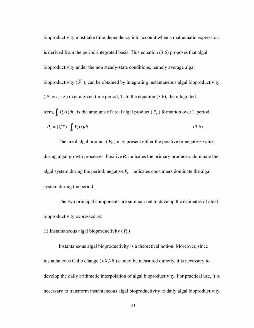
bioproductivity must take time-dependency into account when a mathematic expression

is derived from the period-integrated basis. This equation (3.6) proposes that algal

bioproductivity under the non steady-state conditions, namely average algal

bioproductivity ( rP ), can be obtained by integrating instantaneous algal bioproductivity

( zrP nr ⋅= ) over a given time period, T. In the equation (3.6), the integrated

term, ∫T

r dttP0

)( , is the amounts of areal algal product ( TP ) formation over T period.

∫⋅=T

rr dttPTP0

)()1( (3.6)

The areal algal product ( TP ) may present either the positive or negative value

during algal growth processes. Positive TP indicates the primary producers dominate the

algal system during the period; negative TP indicates consumers dominate the algal

system during the period.

The two principal components are summarized to develop the estimates of algal

bioproductivity expressed as:

(i) Instantaneous algal bioproductivity ( rP )

Instantaneous algal bioproductivity is a theoretical notion. Moreover, since

instantaneous Chl a change ( dtdX ) cannot be measured directly, it is necessary to

develop the daily arithmetic interpolation of algal bioproductivity. For practical use, it is

necessary to transform instantaneous algal bioproductivity to daily algal bioproductivity.

32

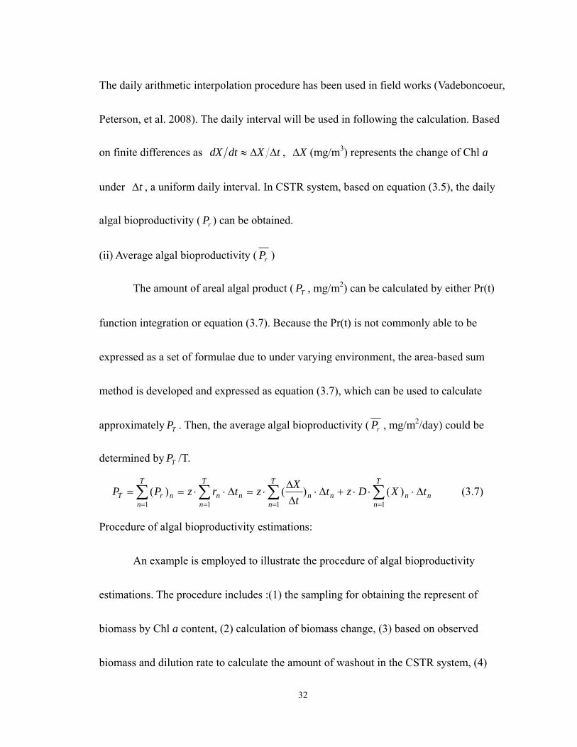
The daily arithmetic interpolation procedure has been used in field works (Vadeboncoeur,

Peterson, et al. 2008). The daily interval will be used in following the calculation. Based

on finite differences as tXdtdX ∆∆≈ , X∆ (mg/m3) represents the change of Chl a

under t∆ , a uniform daily interval. In CSTR system, based on equation (3.5), the daily

algal bioproductivity ( rP ) can be obtained.

(ii) Average algal bioproductivity ( rP )

The amount of areal algal product ( TP , mg/m2) can be calculated by either Pr(t)

function integration or equation (3.7). Because the Pr(t) is not commonly able to be

expressed as a set of formulae due to under varying environment, the area-based sum

method is developed and expressed as equation (3.7), which can be used to calculate

approximately TP . Then, the average algal bioproductivity ( rP , mg/m2/day) could be

determined by TP /T.

n

T

nnn

T

nnn

T

nn

T

nnrT tXDzt

tXztrzPP ∆⋅⋅⋅+∆⋅

∆∆

⋅=∆⋅⋅== ∑∑∑∑==== 1111

)()()( (3.7)

Procedure of algal bioproductivity estimations:

An example is employed to illustrate the procedure of algal bioproductivity

estimations. The procedure includes :(1) the sampling for obtaining the represent of

biomass by Chl a content, (2) calculation of biomass change, (3) based on observed

biomass and dilution rate to calculate the amount of washout in the CSTR system, (4)

33

calculation of nr and plot of the time-varying Pr(t), (5) based on equation (3.7) to

calculate areal algal product ( TP ), and (8) calculate the average algal bioproductivity

( rP ).

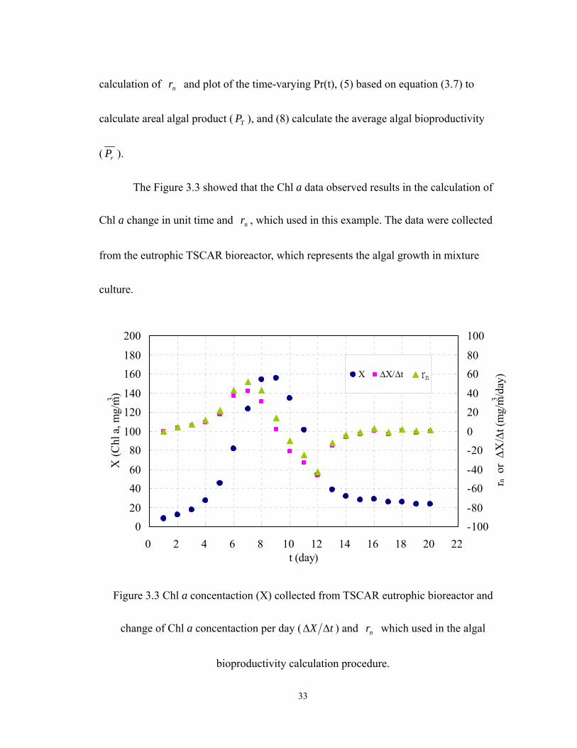
The Figure 3.3 showed that the Chl a data observed results in the calculation of

Chl a change in unit time and nr , which used in this example. The data were collected

from the eutrophic TSCAR bioreactor, which represents the algal growth in mixture

culture.

020

4060

80100

120140

160180

200

0 2 4 6 8 10 12 14 16 18 20 22t (day)

X (C

hl a

, mg/

m3 )

-100-80

-60-40

-200

2040

6080

100

r n o

r ∆X

/∆t (

mg/

m3 /day

)X ∆X/∆t rn

Figure 3.3 Chl a concentaction (X) collected from TSCAR eutrophic bioreactor and

change of Chl a concentaction per day ( tX ∆∆ ) and nr which used in the algal

bioproductivity calculation procedure.

34

1. Monitor X

Replicate samples for X (Chl a, mg/L) are taken which is recommended under

regular interval at 1-day over T period. If an irregular interval is given, use interpolation

to insert an intermediate term in a period of time. The length of T is dependent on the

need of tasks. It can be collected in event base (e.g., algal bloom event), seasonal, or

annual period.

2. Change of Chl a concentration per unit time: tX ∆∆

A set of rate-of-change data was constructed (mg Chl a/m3 /day) by using 1-day

intervals for calculation.

3. Washout term: DX

In CSTR, washout Chl a was determined as dilution rate multiplied by Chl a

concentration at time, t.

4. Instantaneous algal bioproductivity: )(tPr

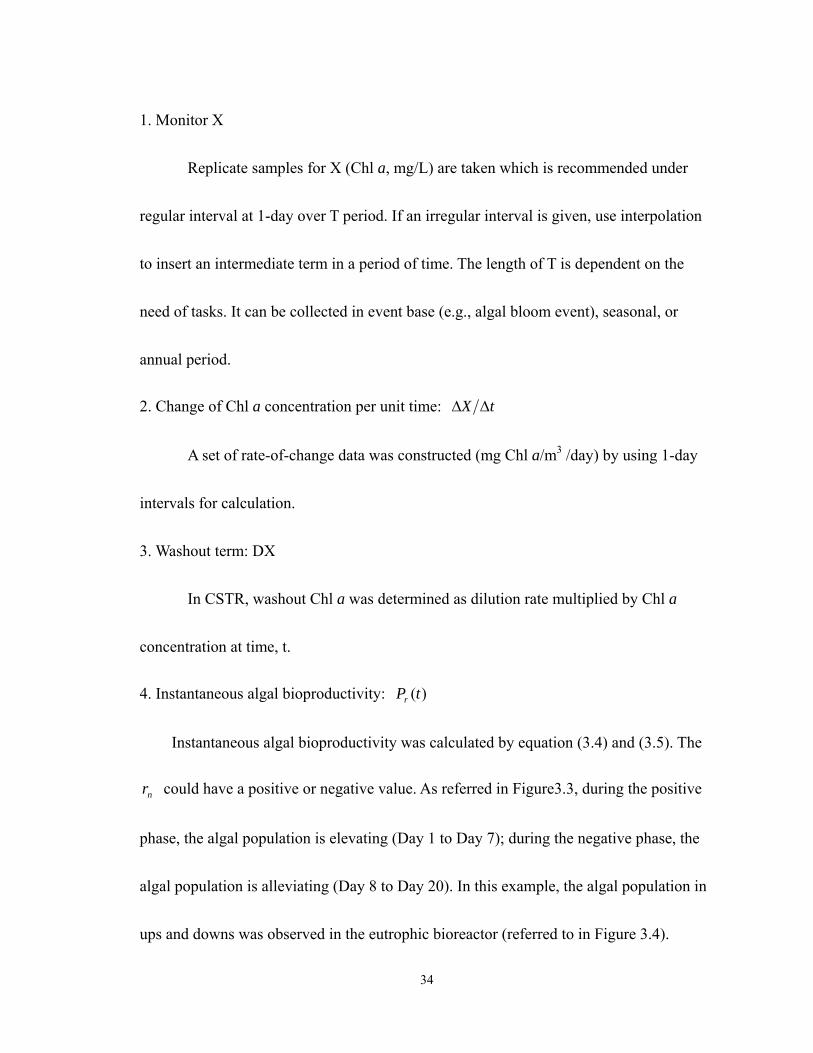
Instantaneous algal bioproductivity was calculated by equation (3.4) and (3.5). The

nr could have a positive or negative value. As referred in Figure3.3, during the positive

phase, the algal population is elevating (Day 1 to Day 7); during the negative phase, the

algal population is alleviating (Day 8 to Day 20). In this example, the algal population in

ups and downs was observed in the eutrophic bioreactor (referred to in Figure 3.4).

35

Figure 3.4 represents the phases in development of algal population. There are two major

phases: accrual phase and loss phase. The change of phases should be caused by either

biochemical compounds or interactions between populations while the environmental and

nutrient conductions are in control of laboratory experiment. Based on the observed data,

)(tPr can be summarized as a set of equations (3.8).

Figure 3.4 Demonstration for algal areal product ( TP , mg/m2) based on )(tPr by using a

set of )(tPr functions (3.8).

⎪⎩

⎪⎨

⎧

=≤≤+

=≤<=

0.985)(R12t7when64.6856.632t-

0.987)(R7t1when478.0)(

2

2535.0 t

r

etP (3.8)

The algal bioproductivity ( rP ) was exponential increase during the period of Day

1 to Day 7; its exponential constant, Kb, was 0.54 (1/day). Following the rP was

36

decreased along the linear track, correlated with time during the period of Day 7 to Day

12. And at Day 9.7 the nr was equal to zero (dX/dt=0). The maximum instantaneous

bioproductivity ( rP ) was 17.2 (mg as Chl a/ m2/day) and occurred on Day 7.

5. Calculate the magnitude of areal algal product ( TP )

Based on step (6), plotted instantaneous bioproductivity ( rP ) versus time (t) showed

as Figure 3.4. With the use of equation (3.7), TP can be calculated approximately. The

area under instantaneous algal bioproductivity )(tPr curve was called areal algal

product ( TP ). The shaded area shows that TP was 34.9 (mg Chl a /m2) which was

calculated by the sum of positive area (+67.3 mg Chl a /m2) and negative area (-32.4 mg

Chl a/m2). Referred to Figure 3.5, the positive area represents that the TP was

accumulating during Day 1 to Day 9. In contrast, the period of the negative area showed

that consumer dominated the system. Finally, TP was maintained at the amounts of

around 34.9 (mg Chl a /m2) for the following seven days.

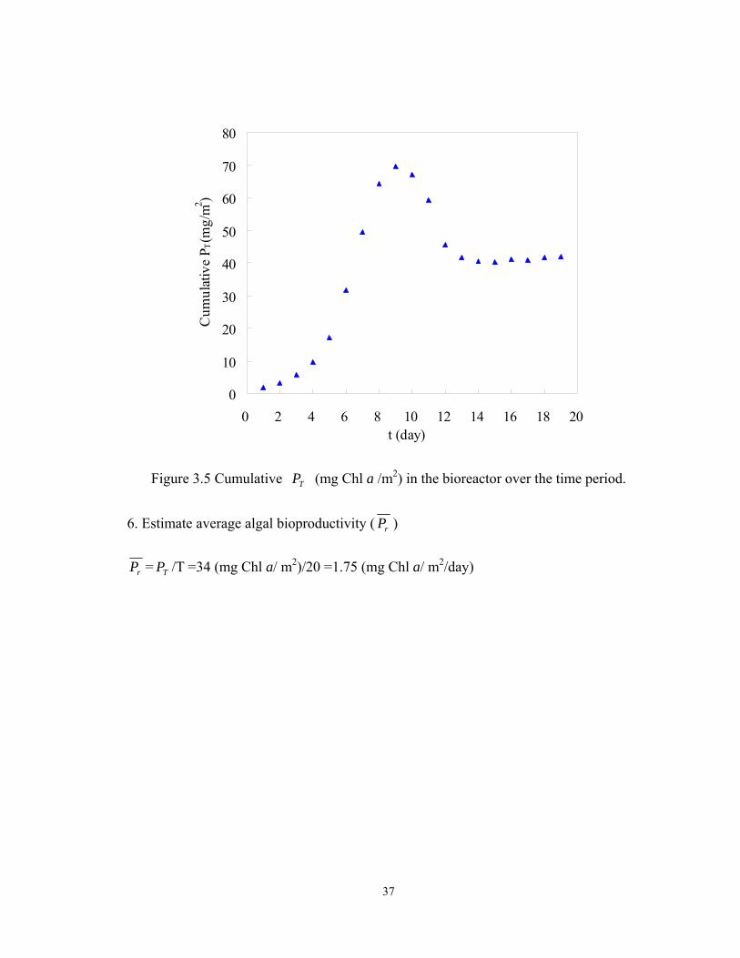
37

0

10

20

30

40

50

60

70

80

0 2 4 6 8 10 12 14 16 18 20t (day)

Cum

ulat

ive

P T(m

g/m2 )

Figure 3.5 Cumulative TP (mg Chl a /m2) in the bioreactor over the time period.

6. Estimate average algal bioproductivity ( rP )

rP = TP /T =34 (mg Chl a/ m2)/20 =1.75 (mg Chl a/ m2/day)

38

3.3 Estimates of lake biodiversity

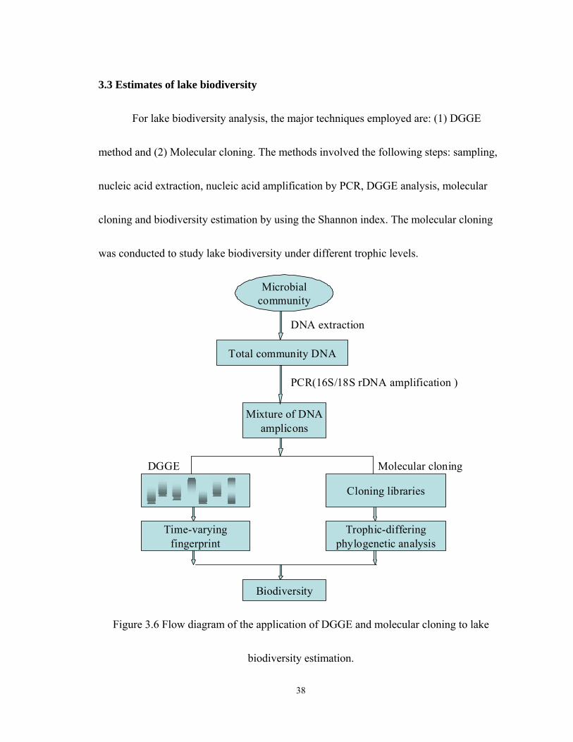
For lake biodiversity analysis, the major techniques employed are: (1) DGGE

method and (2) Molecular cloning. The methods involved the following steps: sampling,

nucleic acid extraction, nucleic acid amplification by PCR, DGGE analysis, molecular

cloning and biodiversity estimation by using the Shannon index. The molecular cloning

was conducted to study lake biodiversity under different trophic levels.

Microbialcommunity

Total community DNA

DNA extraction

Mixture of DNAamplicons

PCR(16S/18S rDNA amplification )

DGGE

Biodiversity

Trophic-differingphylogenetic analysis

Cloning libraries

Molecular cloning

Time-varyingfingerprint

Figure 3.6 Flow diagram of the application of DGGE and molecular cloning to lake

biodiversity estimation.

39

Methods Sampling

Water samples were collected from three TSCARs’ sample receivers during the

experiment period. 300 ml volume of water samples were collected and then immediately

filtered through 0.45 µ m pore-size hydrophilic mixed cellulose ester filter (Pall Life

Science). The filter was kept in 1.7ml microcentrifuge tube (VWR) and stored at -75 oC

until nucleic acid extraction was conducted.

DNA extraction

The CTAB (Cetyl Trimethyl Ammonium Bromide) base protocol of nucleic acid

extraction was used in this research. This was well developed, described as in previous

studies (Lefranc, et al. 2005; Phillips, Celia, et al. 2001). The filters were moved from -75

oC to room temperature for 30 min. Cover the filters with TE buffer (10mM Tris-Cl pH

8.0, 1mM EDTA pH 8.0) and lysozyme solution (final conc., 250µg/ml). The filters were

incubated at 37 oC for 30 min. Add sodium dodecyl sulfate (SDS, 10%) and Proteinase K

(final conc. 100ug/ml) and then incubate at 37 oC for at least one hour. Add CTAB (final

conc. 2% in a 0.7 M NaCl solution) and incubate at 65 oC for 10 min. Transfer the sample

to a new tube (1.7ml microcentrifuge tube). Add an equal volume of phenol: chloroform:

isoamyl alcohol (25:24:1). Mix the contents of the tubes until the emulsion forms.

40

Centrifuge the mixture at 13,000 rpm for one min. Move upper phase to new tube. Add

an equal volume of chloroform mixture (chloroform: isoamyl alcohol (24:1)). Estimate

the volume of the nucleic acid solution. Move 495 µl to new tube and add the 5 µl NaCl

5M (final conc. 0.1M). The final volume is equal to 500 µl. Gently mix the solution. Add

ice-cold ethanol, 2 volumes of nucleic acid solution mixture. Mix solution and store the

ethanolic solution on ice to allow the precipitate of nucleic acid to form. Store the

solution at -20 oC for 4 hours. Centrifuge at 13,000 rpm for 10 min. Fill the tube 1000 µl

with 70% ethanol and re-centrifuge at 13,000 rpm for 2min. Then carefully remove the

supernatant by standing the tube in an inverted position on a wipes layer. Store the open

tube on the bench for 30 min. Add TE (1X) 50µl. The nucleic acid yield was quantified

by a spectrophotometer (Biophotometer 6131, Eppendorf) with a plastic cuvette (10/2

mm, 220-1600nm, UVette, Eppendorf) detecting absorbance at 260nm. The nucleic acid

extracts were stored at -20°C until use.

DGGE analysis

PCR amplification for DGGE experiments

PCR was performed to amplify the specific gene (16S rDNA and 18S rDNA).

After extracting the nucleic acid, the fragment of DNA was performed in a PTC 100

Thermal Cycler (MJ Research) which was automated and programmable equipment. The

41

16S rDNA gene were amplified by the primers of BAC518R (5’ ATT ACC GCG GCT

GCT GCT GG 3’) (Muyzer, G. et al., 1993) and BAC338F+GC (5’ CGC CCG CCG CGC

GCG GCG GGC GGG GCG GGG GCA CGG GGG GAC TCC TAC GGG AGG CAG

CAG 3’) which are specific for most Bacteria, Archaea, and Eucarya. PCR amplification

was performed in a 50 µl volume containing approximately 5 ng of template DNA, 1X

KCl Reaction Buffer (Bioline) containing 50mM KCl, 10mM Tris-HCl pH 8.8 (at 25°C),

1.5mM MgCl2, and stabilizers, 0.2µM primer, 200µM each deoxynucleotide (Bioline),

400 ng of bovine serum albumin (Promega), and 1 U of Taq DNA polymerase (Bioline).

PCR cycling was performed with a PTC 100 Thermal Cycler (MJ Research). The

temperature cycling conditions were as follows: a 5 min initial denaturation at 94°C, 10

cycles of 94°C for 30 s, 55°C for 30 s, and 72°C for 30s, and 25 cycles of 92°C for 30 s,

55°C for 30 s, and 72°C for 30s, followed by 5 min at 72°C and incubation by 2 min at

4°C (Lapara, Nakatsu, et al. 2000). The 18S rDNA gene were amplified by the primers of

F1427GC (5’-CGC CCG CCG CGC CCC GCG CCC GGC CCG CCG CCC CCG CCC

CTC TGT GAT GCC CTT AGA TGT TCT-3’-3’) and R1616 (5’-GCG GTG TGT ACA

AAG GGC AGG G-3’). The primers are specific for eukaryotic aquatic microorganisms

(Van Hannen, Zwart, et al. 1999). The thermal cycling conditions were as follows: 5 min

of initial denaturation at 94°C followed by 25 cycles of 94°C for 1 min, 52°C for 1 min,

42

and 72°C for 1 min and then a final extension step of 72°C for 5 min. The reaction

conditions were as described above.

DGGE experiments

DGGE was performed as described previously (Klammer, Knapp, et al. 2008;

Muyzer, et al. 1993). Briefly, 30µl volume of PCR products were loaded into a

1.5-mm-thick vertical gel containing 8% (w/v) polyacrylamide

(acrylamide-bisacrylamide, 37.5:1) and conducted by the DCode University Mutation

Detection system (BIO-RAD). Two linear gradient denaturing gels were casted for

detecting the migration of DNA fragments. The linear gradient denaturing gels consisted

of urea and deionized formamide (deionized by ion exchange resin, BIO-RAD

G501-X8CD), ascending denatueant from 40% to 60% for the mutation of the 16S rDNA

fragment and from 30% to 55% for the mutation of the 18S rDNA fragment. We prepared

100% denaturant which was defined as 7 M urea and 40% (v/v) formamide (deionized).

Electrophoresis was performed at 60°C in a 0.5X TAE buffer, and 75 V of electricity

(6V/cm) was applied to the gel for 16 hr. DNA were visualized by staining them for 30

min in 3X Gel Green (Biotium) staining solution containing 50 µl Gel Green, 17 ml 1M

NaCl, and 150 ml di-water and then photographing the gel using the Fotodyne system

(FOTODYNE Incorporated, Japan). Digitized images were adjusted by Quantity One

43

4.6.3(BIO-RAD) PC image software.

Molecular Cloning

PCR amplification

PCR was performed with primer EukA (5’-ACCTGGTTGATCCTGCCAG-‘3)

and EukB (5’-TGATCCTTCYGCAGGTTCAC-‘3) (Medlin, Elwood, et al. 1988;

Moon-van der Staay, Staay, et al. 2000), which amplified approximately 1.7kb of

full-length 18S rRNA gene. PCR program involved a 3 min initial denaturation at 94°C

followed by 30 cycles of 94°C for 45 min, 55°C for 1 min, and 72°C for 3 min and then a

final extension step of 72°C for 5 min (Moon-van der Staay, et al. 2001). PCR

amplification was performed in a 50 µl volume containing 1µl DNA extraction product as

template DNA, 1X KCl reaction buffer (Bioline), 1.5mM MgCl2, 0.2mM primer, 0.2mM

each deoxynucleotide (Bioline), and 0.3U of Taq DNA polymerase (Bioline). PCR

cycling was performed with a PTC 100 Thermal Cycler (MJ Research). The 1% low-melt

agarose gel (Promega) was used to recover DNA fragments of PCR product and then

purified by Wizard SV Gel and PCR Clean-up system (Promega) for ligation reaction

use.

Transformations

E.Coli strain DH10B cell were prepared described as in previously study

44

(Sambrook and Russell 2001). The purified PCR products were ligated into the pGEM-T

plasmid vector (Promega, Madison, Wis) and transformed into DH10B cell.

Electroporation were carried out by Electroporator 2510 (Eppendorf, USA) set at 1700 V

pulse discharge. Ligation reactions were performed according to manufacturer’s

recommendations (Promega, Madison, Wis). Clones containing insert DNA of the correct

size were stored in glycerol (15%) at -20 °C for later use.

Clone Libraries

Three eukaryotic libraries (Oligotrophic, mesotrophic and eutrophic bioreactors)

and one prokaryotic library (eutrophic bioreactor) were constructed, designated as Ek4

library (Oligotrophic), Ek5 library (Mesotrophic), Ek6 library (Eutrophic), and Pk6

library (Eutrophic). Around 62 clones from each library were randomly picked from

different LB plates with ampicillin/IPTG/X-Gal. These clones containing insert DNA of

the correct size were picked, incubated at 37 °C overnight and stored in glycerol (15%) at

-20 °C for later use. The size of inserts DNA of 18S /16 S rDNA in positive colonies were

checked by PCR amplification by using primers M13f (5’GT TTT CCC AGT CAC

GAC’3) and M13r (5’CA GGA AAC AGC TAT GAC’3). The correct size of inserts DNA

was amplified by PCR using the primers EK1427f (GC) and EK1616r described

previously. These PCR products were loaded into DGGE gel for screening clone libraries

45

(Kowalchuk, Stephen, et al. 1997; Rowan, Snape, et al. 2003; Van Hannen, et al. 1999). It

provides a pre-filtered strategy for analyzing a numerous clones. The presence of same

position in DGGE gel was be grouped together and considered representative member in

each library (Muyzer and Kornelia 1998).

DNA Sequence

One of insert DNA of each group was sequenced as a representative member. The

plasmid from selected clones were extracted by using Mine-prep protocol (Sambrook and

Russell 2001). The primers Eku A and Eku B were used for sequencing. The sequencing

reactions were carried out by Biotech Core (http://core.biotech.hawaii.edu/default.htm).

Automatic pairwise alignment of all sequences was performed by Bioedit Sequence

Alignment Editor Program (available for download at

http://www.mbio.ncsu.edu/bioedit/bioedit.html).

Phylogenetic analyses

The sequence of three bioreactors were compared to SSU rDNA sequence in

GenBank using BLAST (Basic Local Alignment Search Tool) (Zhang, Schwartz, et al.

2000) analysis to determine their phylogenetic affiliation.

Determination of Biodiversity

DGGE experiments

46

Image of DGGE gel was used to determine the lake biodiversity of three TSCARs

by the Shannon index. The formula of the Shannon index ( 'H ) was published by Claude

E. Shannon (Shannon 1948). The Shannon index is one of the nonparametric measures of

biodiversity based on two assumptions: (1) the individuals are randomly sampled from an

infinite community; (2) all species are represented in the sample (Hutcheson 1970). The

banding data of the DGGE gel was digitized by using the TotalLab software (Nonlinear,

USA). The digital banding data consisted of the number of band and peck height intensity

of band. An example performed by TotalLab is shown as Appendix A which illustrated

the procedure of digitizing bands. Equation (3.9) was used to calculate biodiversity based

on the importance probability of band ( ijp ) at i pixel position on j lane. The ijp (= ji Nn )

was determined by intensity of peck height ( in ) of i th band divided by total peck height

( jN ) of intensity of j th lane (Eichner, Erb, et al. 1999). Based on several assumptions

adopted as described previous studies (Fromin, Hamelin, et al. 2002; Murray, Hollibaugh,

et al. 1996), digital banding data of DGGE gel can be applied in fingerprinting analysis.

For interpreting DGGE fingerprinting, each discrete band of DGGE gel was regarded as a

unique OUT (or phylotype) and the peck height of each band was directly related to

density (or abundance) of OUT (or phylotype) in assemblage (Murray, et al. 1996). Thus,

the banding data obtained from gel image can be applied in the calculation of statistic

47

index of biodiversity (Fromin, et al. 2002). The formula for calculating algal biodiversity

by the Shannon index is:

∑−= ijij ppH ln' (3.9)

ijp =j

i

Nn

(3.10)

SHEln

'

= (3.11)

Where,

'H = Shannon index; ijp = importance probability of band; in = peck height of i th band;

jN = sum of peck height of all band on j th lane; E = Evenness; S = total band count on

one lane.

TotalLab software was used to banding detection of DGGE gel of 18S rDNA

fragments amplified from Lake Wilson water samples from WSFP (gel C) and DSTP (gel

D) stations collected on April 13, 2011 (Refered to Appendix A). Using equaton

(3.9)~(3.11), eukaryotic biodiversity was calculated and shown as Table 4.8. The variance

in biodiversity of two sites can be estimated using the t-test method developed by

Hutcheson (Hutcheson 1970). Hutcheson (Hutcheson 1970) presented a t-test method for

comparing the biodiversity of Shannon index. If absolute t-value is larger than the

two-tailed critical value of t ( dft ),2(α , where α(2) = two-tailed probability ofα; d.f.=

degrees of freedom), it indicated that two sites are significantly different at the 5% level.

48

Based on the DGGE banding data of FigureA.1 in Appendix A, for instance, the

biodiversity of DSTP site was H’=1.725 while the biodiversity of WSFP site was

H’=2.571. The t-test showed that the two sites were significantly different under 5% level

(t=14,α(2) =0.05, d.f.=764).

3.4 Discussion

In order to diagnose and evaluate the performance of bioreactors in terms of the

physical and biological aspects, the tracer experiment and image of DGGE were used.

Tracer experiments can be used to diagnose whether the system was under perfect mixing.

DGGE banding data can be used to evaluate that the species introduced from Lake

Wilson in the artificial system.

Behavior of fluid flowing through the bioreactors

A tracer experiment was conducted in order to determine the flow behavior of this

TSCARs system either under plus flow or well-mixed flow. The three bioreactors were

deviated from the ideal flow model and the operation parameters referred to in Table 3.1.

The tracer experiment was used to confirm the actual system and evaluate the efficiency

of bioreactors. A conservative substance, potassium chloride (KCl), was used as a tracer

in the experiment. The concentration C0 (0.01 M, KCl) of step tracer input was injected

continuously, and the concentration of tracer output (C) and the volumetric rate of

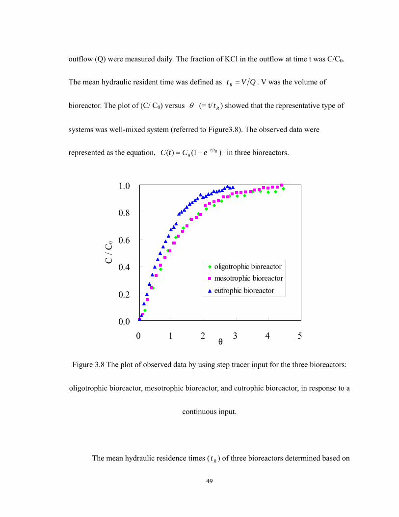
49

outflow (Q) were measured daily. The fraction of KCl in the outflow at time t was C/C0.

The mean hydraulic resident time was defined as QVtR = . V was the volume of

bioreactor. The plot of (C/ C0) versus θ (= t/ Rt ) showed that the representative type of

systems was well-mixed system (referred to Figure3.8). The observed data were

represented as the equation, )1()( 0RtteCtC −−= in three bioreactors.

0.0

0.2

0.4

0.6

0.8

1.0

0 1 2 3 4 5θ

C /

C0

oligotrophic bioreactormesotrophic bioreactoreutrophic bioreactor

Figure 3.8 The plot of observed data by using step tracer input for the three bioreactors:

oligotrophic bioreactor, mesotrophic bioreactor, and eutrophic bioreactor, in response to a

continuous input.

The mean hydraulic residence times ( Rt ) of three bioreactors determined based on

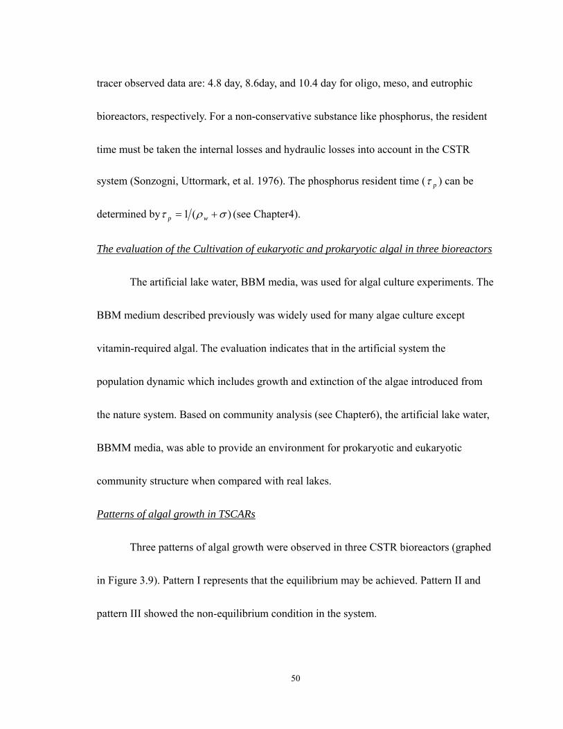
50

tracer observed data are: 4.8 day, 8.6day, and 10.4 day for oligo, meso, and eutrophic

bioreactors, respectively. For a non-conservative substance like phosphorus, the resident

time must be taken the internal losses and hydraulic losses into account in the CSTR

system (Sonzogni, Uttormark, et al. 1976). The phosphorus resident time ( pτ ) can be

determined by )(1 σρτ += wp (see Chapter4).

The evaluation of the Cultivation of eukaryotic and prokaryotic algal in three bioreactors

The artificial lake water, BBM media, was used for algal culture experiments. The

BBM medium described previously was widely used for many algae culture except

vitamin-required algal. The evaluation indicates that in the artificial system the

population dynamic which includes growth and extinction of the algae introduced from

the nature system. Based on community analysis (see Chapter6), the artificial lake water,

BBMM media, was able to provide an environment for prokaryotic and eukaryotic

community structure when compared with real lakes.

Patterns of algal growth in TSCARs

Three patterns of algal growth were observed in three CSTR bioreactors (graphed

in Figure 3.9). Pattern I represents that the equilibrium may be achieved. Pattern II and

pattern III showed the non-equilibrium condition in the system.

51

Figure 3.9 Algae growth patterns observed in three TSCAR bioreactors

52

CHAPTER 4. LAKE BIODIVERSITY UNDER DIFFERENT TROPHIC LEVELS

Lake biodiversity of the different trophic levels was examined by conducting

denaturing gradient gel electrophoresis (DGGE) experiments. In the laboratory, three

trophic states formed in TSCARs based on the total phosphorus loading concept of the

Vollenweider model. This is representative of the trophic states of the lake described in

Chapter 3. DGGE fingerprints of 18 S ribosomal DNA (eukaryote) and 16S ribosomal

DNA (prokaryote) fragments were used to investigate the lake eukaryotic and prokaryotic

biodiversity in samples obtained from TSCARs. On the other hand, a comparative filed

investigation was conducted by sampling from two distinct trophic-state stations of Lake

Wilson. In the field study, the survey in the lake was conducted including the

measurement of water quality such as TP, SRP, TN, TC, TSS, pH, DO, conductivity, and

Chl a. The yield of point and nonpoint sources of TP loading from Lake Wilson

watershed was estimated by the observed data of the Hawaii state government and

Basins/PLoad Model. This case study allowed us to relate the empirical lake biodiversity

to different trophic levels.

4.1 Laboratory investigation

The artificial, simplified algal microcosms used to simulate different trophic states

53

of the lake were common methods in investigating the relationship of trophic level and its

biodiversity (Jardillier, Boucher, et al. 2005; Kassen, Buckling, et al. 2000). Three algal

microcosms formed by TSCARs in the laboratory were regarded as the lakes classified

according to trophic states (oligotrophic, mesotrophic and eutrophic) and then the

biodiversity was examined by DGGE. The details of TSCARs were described in Chapter

3. The results of TSCARs showed that three trophic states were clearly demonstrated

according to TP concentration which is in response to variation in nutrient enrichment.

4.1.1 Results of TSCARs experiments

The TSCARs were designed based on the Vollenweider model (Vollenweider

1976) and this model was expected to predict trophic status in lakes. Based on the

experimental design (referred to Table 3.1), the TSCARs phosphorus-limited system

conducted under two designated parameters: hydraulic overflow rate (q, m/yr) and areal

loading of TP (W’, g/m2/yr) was expected to create the three distinct trophic states

identified by TP concentration as shown Table 4.1.

After replicate experiments, TSCARs formed a sufficient basis for describing the

algal microcosms in which the system presents the attributes of trophic states. In the three

trophic states, algal productivity in the three algal microcosms was estimated and

grouped into three trophic degrees, in which the magnitude of algal bioproductivity

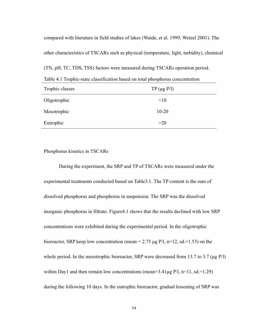
54

compared with literature in field studies of lakes (Waide, et al. 1999; Wetzel 2001). The

other characteristics of TSCARs such as physical (temperature, light, turbidity), chemical

(TN, pH, TC, TDS, TSS) factors were measured during TSCARs operation period.

Table 4.1 Trophic-state classification based on total phosphorus concentration

Trophic classes TP (µg P/l)

Oligotrophic <10

Mesotrophic 10-20

Eutrophic >20

Phosphorus kinetics in TSCARs

During the experiment, the SRP and TP of TSCARs were measured under the

experimental treatments conducted based on Table3.1. The TP content is the sum of

dissolved phosphorus and phosphorus in suspension. The SRP was the dissolved

inorganic phosphorus in filtrate. Figure4.1 shows that the results declined with low SRP

concentrations were exhibited during the experimental period. In the oligotrophic

bioreactor, SRP keep low concentration (mean = 2.75 µg P/l, n=12, sd.=1.53) on the

whole period. In the mesotrophic bioreactor, SRP were decreased from 13.7 to 3.7 (µg P/l)

within Day1 and then remain low concentrations (mean=3.41µg P/l, n=11, sd.=1.29)

during the following 10 days. In the eutrophic bioreactor, gradual lessening of SRP was

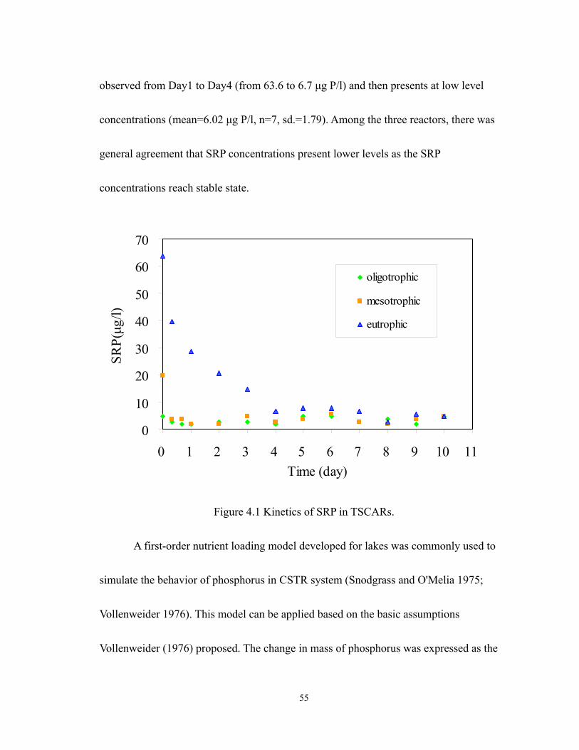
55

observed from Day1 to Day4 (from 63.6 to 6.7 µg P/l) and then presents at low level

concentrations (mean=6.02 µg P/l, n=7, sd.=1.79). Among the three reactors, there was

general agreement that SRP concentrations present lower levels as the SRP

concentrations reach stable state.

0

10

20

30

40

50

60

70

0 1 2 3 4 5 6 7 8 9 10 11Time (day)

SRP(

µg/l)

oligotrophic

mesotrophic

eutrophic

Figure 4.1 Kinetics of SRP in TSCARs.

A first-order nutrient loading model developed for lakes was commonly used to

simulate the behavior of phosphorus in CSTR system (Snodgrass and O'Melia 1975;

Vollenweider 1976). This model can be applied based on the basic assumptions

Vollenweider (1976) proposed. The change in mass of phosphorus was expressed as the

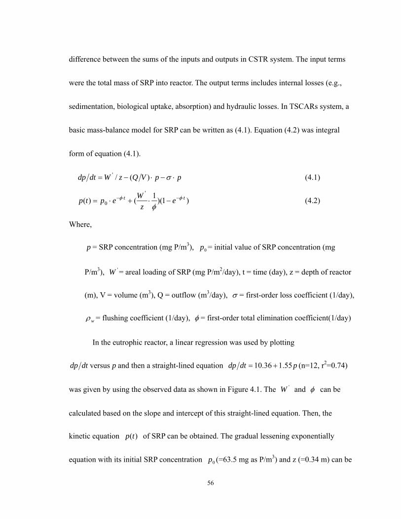
56

difference between the sums of the inputs and outputs in CSTR system. The input terms

were the total mass of SRP into reactor. The output terms includes internal losses (e.g.,

sedimentation, biological uptake, absorption) and hydraulic losses. In TSCARs system, a

basic mass-balance model for SRP can be written as (4.1). Equation (4.2) was integral

form of equation (4.1).

ppVQzWdtdp ⋅−⋅−= σ)(/' (4.1)

)1)(1()('

0tt e

zWeptp ⋅−⋅− −⋅+⋅= φφ

φ (4.2)

Where,

p = SRP concentration (mg P/m3), 0p = initial value of SRP concentration (mg

P/m3), 'W = areal loading of SRP (mg P/m2/day), t = time (day), z = depth of reactor

(m), V = volume (m3), Q = outflow (m3/day), σ = first-order loss coefficient (1/day),

wρ = flushing coefficient (1/day), φ = first-order total elimination coefficient(1/day)

In the eutrophic reactor, a linear regression was used by plotting

dtdp versus p and then a straight-lined equation pdtdp 55.136.10 += (n=12, r2=0.74)

was given by using the observed data as shown in Figure 4.1. The 'W and φ can be

calculated based on the slope and intercept of this straight-lined equation. Then, the

kinetic equation )(tp of SRP can be obtained. The gradual lessening exponentially

equation with its initial SRP concentration 0p (=63.5 mg as P/m3) and z (=0.34 m) can be

57

expressed as )1(68.65.63)( 5502.15502.1 tt eetp ⋅−⋅− −+⋅= . When the t>> phosphorus

residence time (theoretically around 3 times ofφ -1), the exponential terms approached

zero, and the steady-state SRP concentration ( ssp =6.68 mg as P/m3) was given. Because

the mesotrophic and oligotrophic reactors reach steady state within one day, the

first-order loss coefficient (σ ) of mesotrophic and oligotrophic reactors were calculated

as )(tp approaches steady-state concentration ( ssp ). The steady-state

equation: ssp =wz

Wρσ +

⋅1'

can be used to calculateσ (Jones and Bachmann 1976). The

first-order kinetic parameters of SRP in three trophic states were summarized in Table4.2.

58

Table 4.2 Parameters and coefficients of first-order kinetic SRP model in three trophic states based on the data of Figure4.1. Trophic classes 'W

(g as P/m2/yr)ssp

( mg as P/m3) φ

(1/day)

σ

(1/day) wρ

(1/day) Oligotrophic* 0.15 2.75 0.447 0.239 0.208 Mesotrophic* 0.37 3.41 0.877 0.761 0.116 Eutrophic** 1.28 6.68 1.550 1.454 0.096

*: Steady-state equation: ssp = )(1)( 'wzW ρσ +⋅ was used to calculateσ in oligotrophic

and mesotrophic reactors based on experimental treatments. **: Gradual lessening exponentially equation: )1(68.65.63)( 5502.15502.1 tt eetp ⋅−⋅− −+⋅=

was used to calculate 'W , ssp and σ of eutrophic reactor.

***: wρ was calculated by 1/ Rt , and here the hydraulic residence times ( Rt ) of three bioreactors were: 4.8, 8.6, and 10.4 day for oligo, meso, and eutrophic reactors, respectively.

Basically, the trophic state of lakes can be classified by total phosphorus

concentration (Chapra and Tarapchak 1976; Dillon 1975; Vollenweider 1976). It was

proposed that the dividing lines of 10 and 20 (µg P/l) of TP concentrations were lower

and upper tolerance limits for mesotrophic state and based on that lakes can be classified

as three trophic states. In this experiment, the daily concentrations of TP were measured

for three trophic reactors (data as shown Figure 4.2). The mean TP concentration of the

oligotrophic reactor was 7.5 (µg P/l) (n=5, sd.=7.1) below TP tolerance value 10 (µg-P/l),

which was regarded as an oligotrophic state. The mean TP concentration of mesotrophic

reactor was 18.5 (µg P/l) (n=10, sd.=5.9), which falls into the mesotrophic state. And for

59

the eutrophic reactor, it presented around 42.2 (µg P/l) (n=10, sd.=5.7) above 20 (µg P/l)

which is affiliated with an eutrophic state. The observation of TP concentrations in

TSCARs provided the clear evidence, which showed that the treatment of experiments by

regulating the hydraulic overflow rate (q) and areal loading of TP (W’) was able to form

different trophic states identified by TP concentration.

0

10

20

30

40

50

60

0 1 2 3 4 5 6 7 8 9 10 11Time (day)

TP (µ

g/l)

oligotrophic mesotrophic eutrophic

Figure 4.2 Observed data of TP concentration in TSCARs.

Estimates of the algal bioproductivity in three trophic levels

The algal bioproductivity was estimated by using the procedure described in

60

Chapter 3. The algal bioproductivity of three trophic states were estimated by using the

data of Chl a collected from TSCARs (data shown in Figure 4.3). Primary procedures

were described as following:

1. Samples for X (Chl a, mg/L) were taken at 3 or 4 days interval over the period of 20

days. Due to irregular sampling interval, the method of interpolation was used to insert

intermediate value into the sampling interval for calculating daily Chl a change ( dtdX ).

0

10

20

30

40

50

60

70

80

0 2 4 6 8 10 12 14 16 18 20Time (day)

Chl

a (µ

g/l)

Eutrophic Mesotrophic Oligotrophic

Figure 4.3 Chl a concentration observed in TSCARs from Day1 to Day19.

2. Washout terms of three CSTR reactors were calculated by DX. Dilution rate (D) was

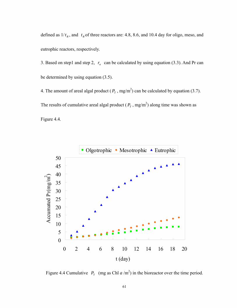
61

defined as 1/ Rt , and Rt of three reactors are: 4.8, 8.6, and 10.4 day for oligo, meso, and

eutrophic reactors, respectively.

3. Based on step1 and step 2, nr can be calculated by using equation (3.3). And Pr can

be determined by using equation (3.5).

4. The amount of areal algal product ( TP , mg/m2) can be calculated by equation (3.7).

The results of cumulative areal algal product ( TP , mg/m2) along time was shown as

Figure 4.4.

05

101520253035404550

0 2 4 6 8 10 12 14 16 18 20

t (day)

Acc

umat

ed P

T(m

g/m2 )

Olgotrophic Mesotrophic Eutrophic

Figure 4.4 Cumulative TP (mg as Chl a /m2) in the bioreactor over the time period.

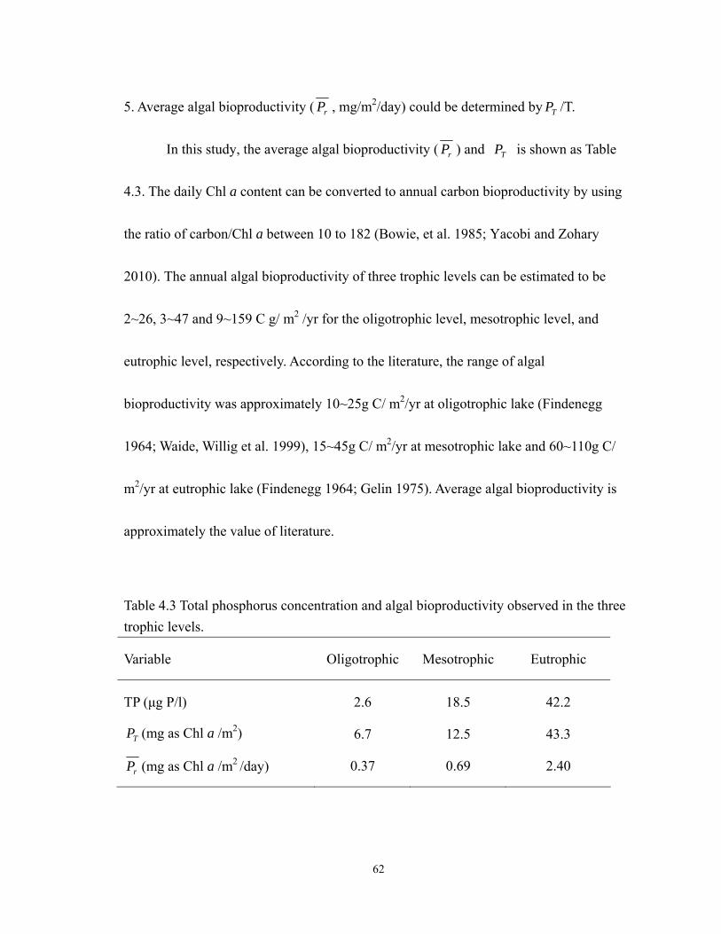
62

5. Average algal bioproductivity ( rP , mg/m2/day) could be determined by TP /T.

In this study, the average algal bioproductivity ( rP ) and TP is shown as Table

4.3. The daily Chl a content can be converted to annual carbon bioproductivity by using

the ratio of carbon/Chl a between 10 to 182 (Bowie, et al. 1985; Yacobi and Zohary

2010). The annual algal bioproductivity of three trophic levels can be estimated to be

2~26, 3~47 and 9~159 C g/ m2 /yr for the oligotrophic level, mesotrophic level, and

eutrophic level, respectively. According to the literature, the range of algal

bioproductivity was approximately 10~25g C/ m2/yr at oligotrophic lake (Findenegg

1964; Waide, Willig et al. 1999), 15~45g C/ m2/yr at mesotrophic lake and 60~110g C/

m2/yr at eutrophic lake (Findenegg 1964; Gelin 1975). Average algal bioproductivity is

approximately the value of literature.

Table 4.3 Total phosphorus concentration and algal bioproductivity observed in the three trophic levels.

Variable Oligotrophic Mesotrophic Eutrophic

TP (µg P/l) 2.6 18.5 42.2

TP (mg as Chl a /m2) 6.7 12.5 43.3

rP (mg as Chl a /m2 /day) 0.37 0.69 2.40

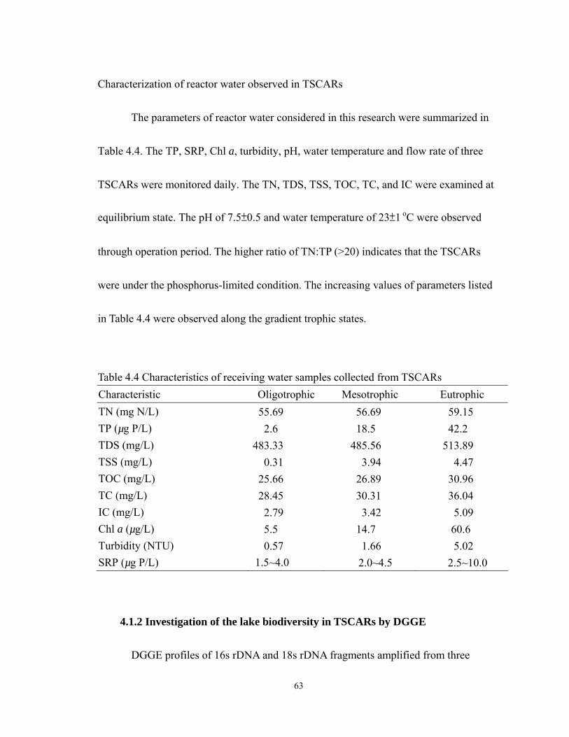
63

Characterization of reactor water observed in TSCARs

The parameters of reactor water considered in this research were summarized in

Table 4.4. The TP, SRP, Chl a, turbidity, pH, water temperature and flow rate of three

TSCARs were monitored daily. The TN, TDS, TSS, TOC, TC, and IC were examined at

equilibrium state. The pH of 7.5±0.5 and water temperature of 23±1 oC were observed

through operation period. The higher ratio of TN:TP (>20) indicates that the TSCARs

were under the phosphorus-limited condition. The increasing values of parameters listed

in Table 4.4 were observed along the gradient trophic states.

Table 4.4 Characteristics of receiving water samples collected from TSCARs Characteristic Oligotrophic Mesotrophic Eutrophic TN (mg N/L) 55.69 56.69 59.15 TP (µg P/L) 2.6 18.5 42.2 TDS (mg/L) 483.33 485.56 513.89 TSS (mg/L) 0.31 3.94 4.47 TOC (mg/L) 25.66 26.89 30.96 TC (mg/L) 28.45 30.31 36.04 IC (mg/L) 2.79 3.42 5.09 Chl a (µg/L) 5.5 14.7 60.6 Turbidity (NTU) 0.57 1.66 5.02 SRP (µg P/L) 1.5~4.0 2.0~4.5 2.5~10.0

4.1.2 Investigation of the lake biodiversity in TSCARs by DGGE

DGGE profiles of 16s rDNA and 18s rDNA fragments amplified from three

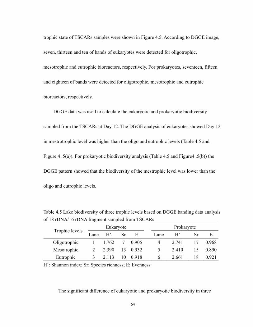
64

trophic state of TSCARs samples were shown in Figure 4.5. According to DGGE image,

seven, thirteen and ten of bands of eukaryotes were detected for oligotrophic,

mesotrophic and eutrophic bioreactors, respectively. For prokaryotes, seventeen, fifteen

and eighteen of bands were detected for oligotrophic, mesotrophic and eutrophic

bioreactors, respectively.

DGGE data was used to calculate the eukaryotic and prokaryotic biodiversity

sampled from the TSCARs at Day 12. The DGGE analysis of eukaryotes showed Day 12

in mestrotrophic level was higher than the oligo and eutrophic levels (Table 4.5 and

Figure 4 .5(a)). For prokaryotic biodiversity analysis (Table 4.5 and Figure4 .5(b)) the

DGGE pattern showed that the biodiversity of the mestrophic level was lower than the

oligo and eutrophic levels.

Table 4.5 Lake biodiversity of three trophic levels based on DGGE banding data analysis of 18 rDNA/16 rDNA fragment sampled from TSCARs

Eukaryote Prokaryote Trophic levels

Lane H’ Sr E Lane H’ Sr E Oligotrophic 1 1.762 7 0.905 4 2.741 17 0.968Mesotrophic 2 2.390 13 0.932 5 2.410 15 0.890

Eutrophic 3 2.113 10 0.918 6 2.661 18 0.921H’: Shannon index; Sr: Species richness; E: Evenness

The significant difference of eukaryotic and prokaryotic biodiversity in three

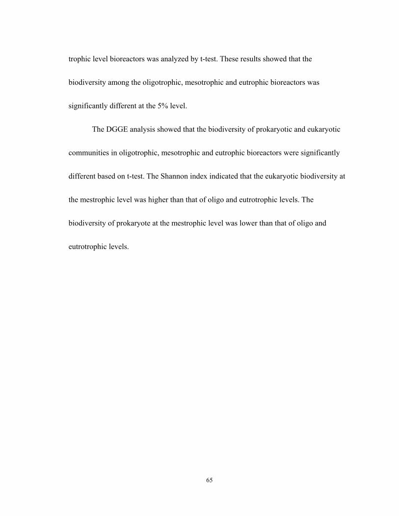
65

trophic level bioreactors was analyzed by t-test. These results showed that the

biodiversity among the oligotrophic, mesotrophic and eutrophic bioreactors was

significantly different at the 5% level.

The DGGE analysis showed that the biodiversity of prokaryotic and eukaryotic

communities in oligotrophic, mesotrophic and eutrophic bioreactors were significantly

different based on t-test. The Shannon index indicated that the eukaryotic biodiversity at

the mestrophic level was higher than that of oligo and eutrotrophic levels. The

biodiversity of prokaryote at the mestrophic level was lower than that of oligo and

eutrotrophic levels.

66

(a)Eukaryote (b)Prokaryote

Figure 4.5 Negative image of DGGE gel of 18/16S rDNA fragment for determining the

biodiversity. Image (a): DGGE analysis of 18S rDNA fragment. Image (b): DGGE

analysis of 16S rDNA fragment. Wahiawa reservoir sample collected on 26 Nov. 2008.

lane1, lane2, and lane3 showed the DGGE band of 18S rDNA fragment collected from

oligotrophic, mesotrophic, and eutrophic bioreactor which samples collected on Day12.

lane4, lane5, lane6 showed DGGE band of of 16S rDNA fragmen from oligotrophic,

mesotrophic, and eutrophic bioreactor collected on Day12.

67

4.2 Field investigation

Lake Wilson was selected as a study site for examining the relationship between

lake biodiversity and trophic levels. Based on the literature, several studies had been

conducted about 30 years ago for Lake Wilson. It provided an overview for Lake Wilson

(Lum and Young 1976; Moore, Lowry, et al. 1981; Young, Dugan, et al. 1975). Lake

Wilson has a maximum capacity of 14.2 × 106 m3, watershed area around 41.4 km2, a

water surface area of around 1.2 km2 at maximum water level, mean depth of 8 m and a

flushing time of 73 days (Young, et al. 1975). The dam withholds the impounded water

from the North and South Forks of the Kaukonahua stream. Recently, several

investigations were conducted in order to develop the TMDLs (Total Maximum Daily

Loads) of pollutants into Lake Wilson. The yield of pollutants (TP, TN, and TSS) from

the North and South Forks of the Kaukonahua watershed were estimated by Tetra Tech

(Tetra Tech 2009; Tetra Tech 2006). According to the water quality standards

classification, Lake Wilson was classified as Class 2 which permitted the use of water for

recreational purposes, propagation of fish and other aquatic life and as agricultural and

industrial water supply (State of Hawaii 2004). Although previous investigations

provided the informed description of Lake Wilson, the lake biodiversity was poorly

known.

68

4.2.1 Results of field investigation in Lake Wilson

On 26 Nov. 2008, a lake-wide survey conducted by dry season sampling at six

locations of Lake Wilson exhibited spatial variation shown in Table1.1. The preliminary

results will serve to illustrate the locations selected for investigating lake biodiversity.

The TP concentration of six locations was under higher concentration (range from 42.2 to

89.1 (µg P /L)). The highest TN peak was observed at DSTP (Downstream of Sewage

Treatment Plant) station. Moving upstream of South Fork Koukonahua from DSTP to

SFKS1 (South Fork Koukonahua station 1), there was a decrease in TN. It was possible

that the effluent contributed the sufficient nitrogen nutrient to the lake from the sewage

treatment plant. The rainfall condition and water level of Lake Wilson were monitored by

two USGS stations: USGS SF Kaukonahua rain gage and USGS 16210000 Wahiawa

Reservoir at Spillway. Sampling date 26 Nov. 2008 was considered under dry weather

and lower water levels. According to USGS SF Kaukonahua rain gauge, there was no

effective rainfall to cause a runoff into receiving water body prior to 72 hrs of the

sampling date 26 Nov. 2008. Reservoir gauge height was 21 m based on USGS 16210000

Wahiawa Reservoir at Spillway at Wahiawa dam.

According to the survey of 26 Nov. 2008, there were spatial variably ratio of

TN:TP, ratio of TC:TP, and Chl a:TOC ratio in the lake water. The ratio of TC:TP was

69

higher than 27 at all monitored locations. The ratio of TN:TP was higher than 7.2 at two

locations: 1) Wahiawa State Freshwater Park and, 2) downstream of Wahiawa Wastewater

Treatment Plant (WWTP). Chl a-to-TOC ratio ranges from 9.0 to 0.8 (µg Chl a/mg C).

This observed data (Table 1.1) released the information regarding the spatial scale

difference of the limiting nutrient. In general, the higher TN:TP ratio >7.2 indicates that

phosphorus was the limited element regulating algal growth in lake water (Chapra 1997).

This implies that phosphorus limited the algal bioproductivity near the outfall of the

sewage treatment plant due to the TN:TP ratio being higher than 7.2. That suggests that

phosphorus regulates the algal growth in two locations of Lake Wilson.

As a conclusion, several reasons were considered for Lake Wilson as a study site

to examine the relationship between lake biodiversity and trophic levels. Firstly, Lake

Wilson is regarded as an eutrophic lake, and its eutrophic state is caused by enriched

nutrients from the point source (effluent of sewage treatment plant) and non-point source.

Secondly, a hypothesis was proposed that trophic levels gradually increases downstream

of Lake Wilson due to significant nutrient contribution from the sewage treatment plant

and longer hydraulic retention time downstream of Lake Wilson. Finally, the Lake Wilson

watershed had been installed with rain and flow gauge stations and then provided

long-term monitored data for analysis.

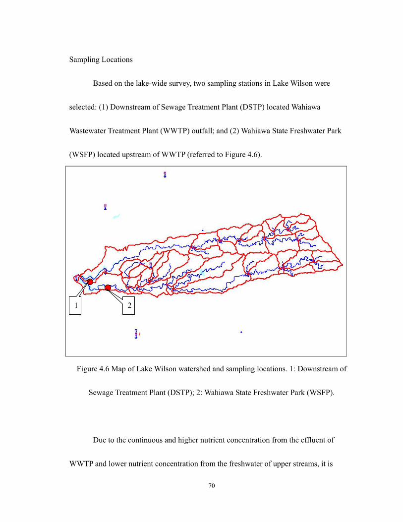
70

Sampling Locations

Based on the lake-wide survey, two sampling stations in Lake Wilson were

selected: (1) Downstream of Sewage Treatment Plant (DSTP) located Wahiawa

Wastewater Treatment Plant (WWTP) outfall; and (2) Wahiawa State Freshwater Park

(WSFP) located upstream of WWTP (referred to Figure 4.6).

Figure 4.6 Map of Lake Wilson watershed and sampling locations. 1: Downstream of

Sewage Treatment Plant (DSTP); 2: Wahiawa State Freshwater Park (WSFP).

Due to the continuous and higher nutrient concentration from the effluent of

WWTP and lower nutrient concentration from the freshwater of upper streams, it is

2 1

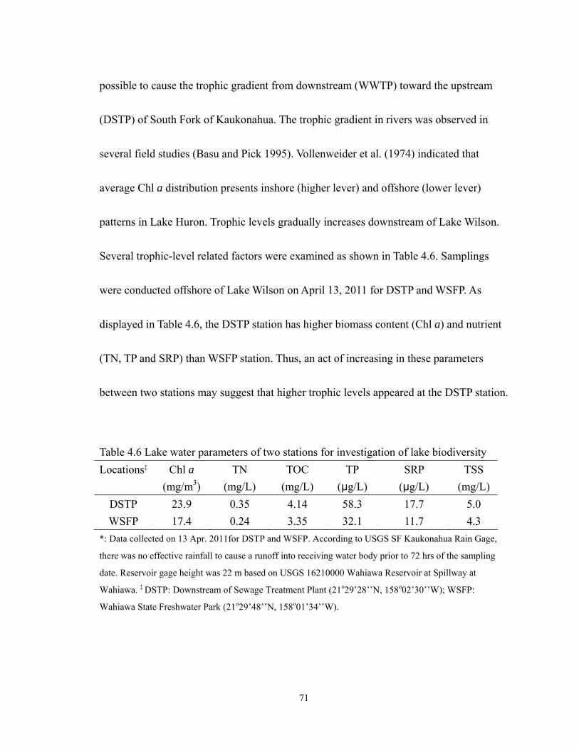
71

possible to cause the trophic gradient from downstream (WWTP) toward the upstream

(DSTP) of South Fork of Kaukonahua. The trophic gradient in rivers was observed in

several field studies (Basu and Pick 1995). Vollenweider et al. (1974) indicated that

average Chl a distribution presents inshore (higher lever) and offshore (lower lever)

patterns in Lake Huron. Trophic levels gradually increases downstream of Lake Wilson.

Several trophic-level related factors were examined as shown in Table 4.6. Samplings

were conducted offshore of Lake Wilson on April 13, 2011 for DSTP and WSFP. As

displayed in Table 4.6, the DSTP station has higher biomass content (Chl a) and nutrient

(TN, TP and SRP) than WSFP station. Thus, an act of increasing in these parameters

between two stations may suggest that higher trophic levels appeared at the DSTP station.

Table 4.6 Lake water parameters of two stations for investigation of lake biodiversity Locations‡ Chl a

(mg/m3) TN

(mg/L) TOC

(mg/L) TP

(:g/L) SRP

(:g/L) TSS

(mg/L)DSTP 23.9 0.35 4.14 58.3 17.7 5.0 WSFP 17.4 0.24 3.35 32.1 11.7 4.3

*: Data collected on 13 Apr. 2011for DSTP and WSFP. According to USGS SF Kaukonahua Rain Gage,

there was no effective rainfall to cause a runoff into receiving water body prior to 72 hrs of the sampling

date. Reservoir gage height was 22 m based on USGS 16210000 Wahiawa Reservoir at Spillway at

Wahiawa. ‡ DSTP: Downstream of Sewage Treatment Plant (21o29’28’’N, 158o02’30’’W); WSFP:

Wahiawa State Freshwater Park (21o29’48’’N, 158o01’34’’W).

72

Profile of DO and temperature at three study sites

Dissolved oxygen (DO) content is the fundamental characteristic of lakes because

photosynthetic production could be estimated by DO (Chapra 1997; Odum 1956; Wetzel

2001). Varying trophic levels related to diurnal cycle of DO curves have been proposed

and investigated in rivers and lakes (Odum 1956; Wang, et al. 2003). The vertical

distribution of DO patterns were found during the four seasons of different trophic level

lakes. The vertical distribution of DO of Lake Wilson was investigated by Moore et al.

(Moore, et al. 1981).

In this study, a real-time approach was used to measure DO variation in two study

locations. YSI 600R DO Sonde (Yellow Springs, Ohio) was used to measure nearly

instantaneous DO in situ. The DO data collected on April 13, 2011 in DSTP and WSFP.

As shown in Figure4.7, the DO vertical profile presents that the higher clino-grade

oxygen curve in DSTP than WSFP of Lake Wilson. The lower zone (depth 6-10m) of

DSTP was an anaerobic environment and DO content increased to 9.5mg/l at the upper

zone (depth 3m). This indicated that the lower zone of this site (DSTP) may have

intensive biochemical oxidation processes in the very productive water.

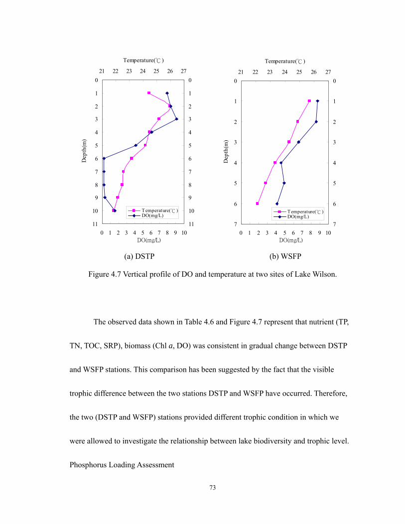
73

0

1

2

3

4

5

6

7

8

9

10

11

21 22 23 24 25 26 27

Temperature(℃)

Dep

th(m

)0

1

2

3

4

5

6

7

8

9

10

110 1 2 3 4 5 6 7 8 9 10

Temperature(℃)DO(mg/L)

DO(mg/L)

0

1

2

3

4

5

6

7

21 22 23 24 25 26 27

Temperature(℃)

Dep

th(m

)

0

1

2

3

4

5

6

70 1 2 3 4 5 6 7 8 9 10

Temperature(℃)DO(mg/L)

DO(mg/L)

(a) DSTP (b) WSFP

Figure 4.7 Vertical profile of DO and temperature at two sites of Lake Wilson.

The observed data shown in Table 4.6 and Figure 4.7 represent that nutrient (TP,

TN, TOC, SRP), biomass (Chl a, DO) was consistent in gradual change between DSTP

and WSFP stations. This comparison has been suggested by the fact that the visible

trophic difference between the two stations DSTP and WSFP have occurred. Therefore,

the two (DSTP and WSFP) stations provided different trophic condition in which we

were allowed to investigate the relationship between lake biodiversity and trophic level.

Phosphorus Loading Assessment

74

In this research, PLOAD/BASINS4.0 (Pollutant Load/ Better Assessment Science

Integrating point & Non-point Sources) was used to estimate TP non-point source

pollutants loading from watershed contributed to Lake Wilson. Annual pollutant loads

can be calculated for each watershed using simple methods in the model of

PLOAD/BASINS 4.0 (USEPA). The governing equation of simple methods is: LP = ∑

(Rf * PJ* RVU * CU* AU * 2.72 / 12). Where, LP = Pollutant load (lbs), Rf = Precipitation

(inches/year), PJ = Ratio of storms producing runoff (default = 0.9), RVU= Runoff

coefficient for land use type u, (runoff inches /inches rainfall), CU = Event Mean

Concentration for land use type u (mg/l), AU = Area of land use type u (acres).

The input data for PLOAD included GIS (Geographic Information Systems) data

and tabular date. Digital data of GIS such as a watershed boundary, stream, digital

elevation model (DEM), and land use can be downloaded from the database of Hawaii

government and USEPA (http://hawaii.gov/dbedt/gis/download.htm). As displayed in the

results in Table 4.7, the yield of TP from the non-point source was 3.1 (tn/yr) and from

point source was 3.5 (tn/yr). This is based on surface area 1.2 km2 of Lake Wilson, the

areal loading of TP (W’, g/m2/yr) was 5.5 (g/m2/yr).

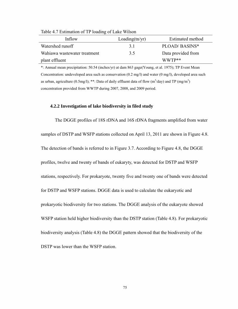
75

Table 4.7 Estimation of TP loading of Lake Wilson Inflow Loading(tn/yr) Estimated method

Watershed runoff 3.1 PLOAD/ BASINS* Wahiawa wastewater treatment plant effluent

3.5 Data provided from WWTP**

*: Annual mean precipitation: 50.54 (inches/yr) at dam 863 gage(Young, et al. 1975); TP Event Mean

Concentration: undeveloped area such as conservation (0.2 mg/l) and water (0 mg/l), developed area such

as urban, agriculture (0.5mg/l); **: Data of daily effluent data of flow (m3/day) and TP (mg/m3)

concentration provided from WWTP during 2007, 2008, and 2009 period.

4.2.2 Investigation of lake biodiversity in filed study

The DGGE profiles of 18S rDNA and 16S rDNA fragments amplified from water

samples of DSTP and WSFP stations collected on April 13, 2011 are shown in Figure 4.8.

The detection of bands is referred to in Figure 3.7. According to Figure 4.8, the DGGE

profiles, twelve and twenty of bands of eukaryty, was detected for DSTP and WSFP

stations, respectively. For prokaryote, twenty five and twenty one of bands were detected

for DSTP and WSFP stations. DGGE data is used to calculate the eukaryotic and

prokaryotic biodiversity for two stations. The DGGE analysis of the eukaryote showed

WSFP station held higher biodiversity than the DSTP station (Table 4.8). For prokaryotic

biodiversity analysis (Table 4.8) the DGGE pattern showed that the biodiversity of the

DSTP was lower than the WSFP station.

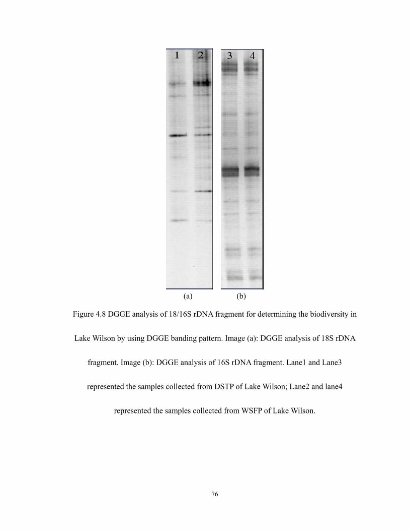
76

(a) (b)

Figure 4.8 DGGE analysis of 18/16S rDNA fragment for determining the biodiversity in

Lake Wilson by using DGGE banding pattern. Image (a): DGGE analysis of 18S rDNA

fragment. Image (b): DGGE analysis of 16S rDNA fragment. Lane1 and Lane3

represented the samples collected from DSTP of Lake Wilson; Lane2 and lane4

represented the samples collected from WSFP of Lake Wilson.

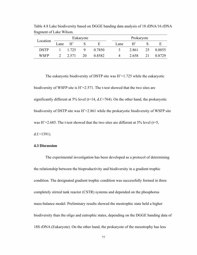
77

Table 4.8 Lake biodiversity based on DGGE banding data analysis of 18 rDNA/16 rDNA fragment of Lake Wilson.

Eukaryote Prokaryote Location

Lane H’ S E Lane H’ S E DSTP 1 1.725 9 0.7850 3 2.861 25 0.8855WSFP 2 2.571 20 0.8582 4 2.658 21 0.8729

The eukaryotic biodiversity of DSTP site was H’=1.725 while the eukaryotic

biodiversity of WSFP site is H’=2.571. The t-test showed that the two sites are

significantly different at 5% level (t=14, d.f.=764). On the other hand, the prokaryotic

biodiversity of DSTP site was H’=2.861 while the prokaryotic biodiversity of WSFP site

was H’=2.685. The t-test showed that the two sites are different at 5% level (t=5,

d.f.=1391).

4.3 Discussion

The experimental investigation has been developed as a protocol of determining

the relationship between the bioproductivity and biodiversity in a gradient trophic

condition. The designated gradient trophic condition was successfully formed in three

completely stirred tank reactor (CSTR) systems and depended on the phosphorus

mass-balance model. Preliminary results showed the mestrophic state held a higher

biodiversity than the oligo and eutrophic states, depending on the DGGE banding data of

18S rDNA (Eukaryote). On the other hand, the prokaryote of the mesotrophy has less

78

biodiversity than the oligo and eutrophic states. The DGGE analysis showed that the

biodiversity of prokaryotic and eukaryotic communities in oligotrophic, mesotrophic and

eutrophic bioreactors are significantly different based on the t-test.

The algal bioproductivity often was expressed as either the content of Chl a

(Ryther and Yentsch 1957) or by the rate of production (Schallenberg 1997). Some

research works showed that high Chl a was not guaranteed to reflect high bioproductivity

because it can be merely the result of accumulation of biomass (Chl a). Therefore, it is

necessary that algal bioproductivity should be defined as a rate term and be the amount of

carbon fixed in unit area per unit time through photosynthesis. In this study, the average

algal bioproductivity (average Pr) can be converted to annual carbon bioproductivity by

using the ratio of carbon/Chl a between 10 to 182 (Bowie, et al. 1985; Yacobi and Zohary

2010). Experiment results showed that the average algal bioproductivity of three trophic

levels, oligotrophic, mesotrophic, and eutrophic levels were 0.4, 0.7 and 2.4 mg as Chl a

/m2 /day, respectively. The annual bioproductivity of three trophic levels can be estimated

to be 2~26, 3~47 and 9~159 C g/m2 /yr for the oligotrophic level, mesotrophic level, and

eutrophic level, respectively. According to the literature, the range of algal

bioproductivity was approximately 10~25g C/m2/yr at oligotrophic lakes (Findenegg

1964; Waide, et al. 1999), 15~45g C/m2/yr at mesotrophic lakes and 60~110g C/m2/yr at

79

eutrophic lakes (Findenegg 1964; Gelin 1975). Average algal bioproductivity was

approximately the value of literature.

80

CHAPTER 5. LAKE BIODIVERSITY WITH TIME VARYING ALGAL

BIOPRODUCTIVITY

Chapter 5 illustrates that lake biodiversity was regulated by algal bioproductivity

during the period of varying algal growth phases, carried out in an eutrophic TSCAR.

The experiment was conducted during 20 days of time-varying observation on mixture

culture in algal bloom. This observation can be used to demonstrate the correlation

between lake biodiversity and algal bioproductivity. In this eutrophic TSCAR, an algal

bloom has been induced by the treatment described in Chapter 3. DGGE fingerprinting

technique was employed to investigate the lake biodiversity along temporal variation in

terms of varying algal bioproductivity during 20 days of laboratory experiment. The

evidence indicates that lake biodiversity can be displayed with time variation in algal

bioproductivity. Consequently, there is a general trend that when data were plotted by

eukaryotic biodiversity (H’) against algal bioproductivity (Pr), the relationship was

positive relation following hump-shaped pattern, whereas when data were plotted by

prokaryotic biodiversity (H’) against algal bioproductivity (Pr), the relationship was

negative relation following U-shaped patterns. Several critical timing points of algal

growth in terms of time-varying Pr(t) revealed a shift in lake biodiversity.

81

5.1 General variation in biodiversity

Many hypotheses attempting to explain the biodiversity variation have recently

been reviewed by Connell and Orias (Connell and Orias 1964), Waide et al. (Waide, et al.

1999), Fukami and Morin (Fukami and Morin 2003) and Smith (2007). These hypotheses

have been examined and account to the interactive effects between the biodiversity and

its environmental conditions. Indeed, biodiversity is regulated by many factors such as

global loss (latitudinal gradient), climatic change (precipitation), spatial factor

(heterogeneity), availability of nutrient, and solar energy (primary bioproductivity)

(Pianka 1966). The relationship between the biodiversity and the bioproductivity attracted

more attention in the biodiversity studies of Pianka. The biodiversity can either positively

or negatively be corrected with bioproductivity (Fukami and Morin 2003; Kassen, et al.

2000; Morin 2000). In fact, six patterns of the biodiversity-bioproductivity were observed

and summarized from experiment of laboratory and natural environment: random,

positive, flat, negative, hump-shaped, and U-shaped (Smith 2007; Waide, et al. 1999).

The hump-shaped relationship of biodiversity-bioproductivity is a widely observed

pattern in which the peak of diversity is at the intermediate bioproductivity level (Kassen,

et al. 2000).

In this study, the hypothesis that “the algal bioproductivity correlates closely with

82

lake biodiversity” was examined to explain if the general patterns of

biodiversity-bioproductivity were caused due to competition for limited nutrients in an

eutrophic freshwater lake. With time-varying analysis, it provided interpretation that the

man-made influx of nutrient often resulted in not only a decrease of eukaryotic

biodiversity but also an increase of prokaryotic biodiversity.

5.2 Results of a time-varying experiment on the eutrophic TSCAR

According to the laboratory experiments described previously (Chapter 3), the

eutrophic environment was formed and the most of the members of phytoplankton were

able to reproduce and build up the algal population in the TSCAR bioreactor. The daily

change of Chl a concentration was measured and the bioproductivity can be calculated by

using the CSTR mass balance equation.

In order to investigate the algal bioproductivity and lake biodiversity, TSCAR

bioreactors were designed and constructed in a laboratory scale experiment. An

experiment was conducted from Sept 23, 2011 through Oct. 4, 2011 in three different

trophic-level TSCAR bioreactors. The samples of TSCARs in oligotrophic, mesotropnic

(data not shown in this chapter) and eutrophic TSCAR bioreactors were collected and

analyzed. The eutrophic TSCAR bioreactor has been set for the initial condition of the

concentration of 60:g as P/l limited-phosphorus nutrient in culture mediums which

83

operated under the conditions shown in Table 3.1. These conditions were designed to

simulate the lake-like eutrophic environment. The SRP and Chl a were measured.

Moreover, samples for DNA extraction of the eukaryotic and prokaryotic DGGE

experiment were collected under a daily interval. In this experiment, an algal bloom in

eutrophic TSCAR was observable and its algal bioproductivity was estimated by Chl a in

the CSTR system during 20 days period. The 12-day time-varying lake biodiversity was

investigated by DGGE profile.

5.2.1 Algal bloom in eutrophic TSCAR

An observation of algal bloom process can be used to exhibit the change of lake

biodiversity along with algal population growth phases in one CSTR system where

regarded as a lake-like microcosm. It could be an example to demonstrate that the

relationship of lake biodiversity and algal bioproductivity in controlled CSTR system,

eutrophic TSCAR bioreactor. A typical algal bloom was formed based on the treatment of

Table3.1 and algal X (mg as Chl a/ m3) against time (t, Day) was plotted shown as Figure

5.1.

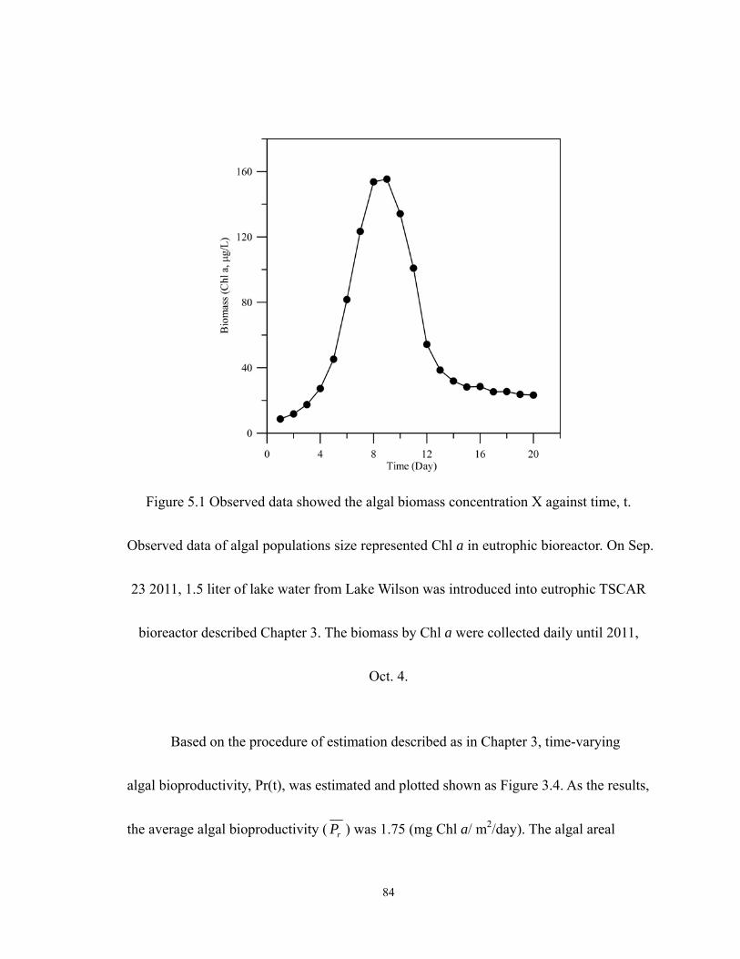
84

Figure 5.1 Observed data showed the algal biomass concentration X against time, t.

Observed data of algal populations size represented Chl a in eutrophic bioreactor. On Sep.

23 2011, 1.5 liter of lake water from Lake Wilson was introduced into eutrophic TSCAR

bioreactor described Chapter 3. The biomass by Chl a were collected daily until 2011,

Oct. 4.

Based on the procedure of estimation described as in Chapter 3, time-varying

algal bioproductivity, Pr(t), was estimated and plotted shown as Figure 3.4. As the results,

the average algal bioproductivity ( rP ) was 1.75 (mg Chl a/ m2/day). The algal areal

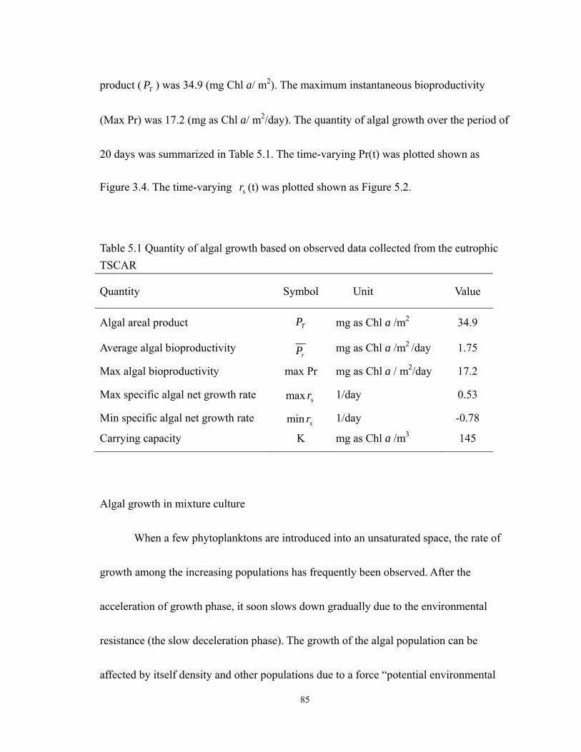
85

product ( TP ) was 34.9 (mg Chl a/ m2). The maximum instantaneous bioproductivity

(Max Pr) was 17.2 (mg as Chl a/ m2/day). The quantity of algal growth over the period of

20 days was summarized in Table 5.1. The time-varying Pr(t) was plotted shown as

Figure 3.4. The time-varying sr (t) was plotted shown as Figure 5.2.

Table 5.1 Quantity of algal growth based on observed data collected from the eutrophic TSCAR

Quantity Symbol Unit Value

Algal areal product TP mg as Chl a /m2 34.9

Average algal bioproductivity rP mg as Chl a /m2 /day 1.75

Max algal bioproductivity max Pr mg as Chl a / m2/day 17.2

Max specific algal net growth rate max sr 1/day 0.53

Min specific algal net growth rate min sr 1/day -0.78

Carrying capacity K mg as Chl a /m3 145

Algal growth in mixture culture

When a few phytoplanktons are introduced into an unsaturated space, the rate of

growth among the increasing populations has frequently been observed. After the

acceleration of growth phase, it soon slows down gradually due to the environmental

resistance (the slow deceleration phase). The growth of the algal population can be

affected by itself density and other populations due to a force “potential environmental

86

resistance” that acts to retard growth. The potential environmental resistance may result

from competition to gain the limited nutrient and predation or grazing process by other

species. The classification of algal growth phases was plotted based on algal net growth

rate ( sr ) referred to in Figure 5.2. When the algal populations complete their growth

(Phase I and Phase II), algal population density in terms of algal biomass (X) tends to

decline below the carrying capacity (K) level which moves towards phase III. The lake

biodiversity of three phases (phase I, phase II and phase III) was investigated in order to

realize the lake biodiversity variation in algal bioproductivity.

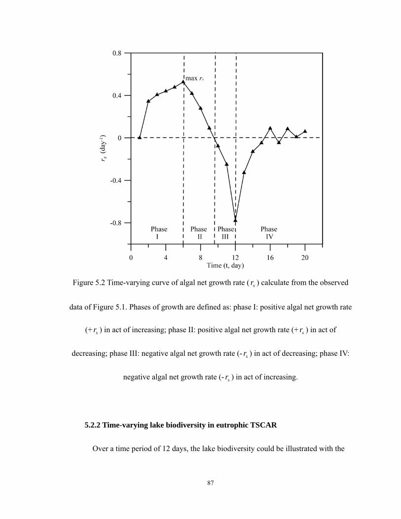
87

Figure 5.2 Time-varying curve of algal net growth rate ( sr ) calculate from the observed

data of Figure 5.1. Phases of growth are defined as: phase I: positive algal net growth rate

(+ sr ) in act of increasing; phase II: positive algal net growth rate (+ sr ) in act of

decreasing; phase III: negative algal net growth rate (- sr ) in act of decreasing; phase IV:

negative algal net growth rate (- sr ) in act of increasing.

5.2.2 Time-varying lake biodiversity in eutrophic TSCAR

Over a time period of 12 days, the lake biodiversity could be illustrated with the

88

images of DGGE gel shown as Figure 5.3 for prokaryotic biodiversity and Figure 5.4 for

eukaryotic biodiversity. The lake biodiversity was investigated with the variation of algal

bioproductivity based on observed data of Figure 5.1. During the 12-day period

(excluding Day3), DGGE image demonstrated the time-varying fingerprinting of the lake

biodiversity in terms of prokaryotic and eukaryotic biodiversity under phase I, phase II,

and phase III. The three phases are in conjunction with an algal blooming. The banding

data of DGGE gel is used to determine the prokaryotic and eukaryotic biodiversity by

Shannon index (Fromin, et al. 2002; Shannon 1948). The banding data of DGGE gel was

digitized by using the TotalLab software (Nonlinear, USA). The digital banding data

transformed from DGGE gel image consisted of the number of band (S) and peck height

( in ) of i th band on j th lane. The Shannon index ( 'H ) and evenness (E) were calculated as

described in Chapter 3.

(i) prokaryotic biodiversity

For comparison, the banding data found for 11 samples collected from eutrophic

TSCAR under the period of 12-day period. As the Figure 5.3 indicates, the variations in

bands were described as present, absent, gradually increasing and decreasing pixel

intensity along each day of the experiment. Nine bands are interested and excised which

marked a, b, c, d, e, f, g, h and i in Figure 5.3. Band a, band b, and band c with the high

89

intensity of pixel can be regarded as dominant bands. Band a was present from Day 1 to

Day10 and with less intensity on Day 9 to Day 10; Band b was present from Day 1 to

Day 12 and became less on Day 12; band c was present on Day 10 to Day 12 and became

less on Day 12; band d was present on Day 4 to Day 6; band e was present on Day 2 to

Day 12 and on Day 12 had higher intensity; band f was present and had gradually

decreasing band intensity from Day 1 to Day 6; band g was present and had gradually

increasing band intensity from Day 1 to Day 12; band h was present on Day 12; band i

was present on Day 5, 6, 7 and Day 12.

The implication of the variation in bands over 12 days is that the band a and band

b may highly relate to Chl a biomass due to gradually increasing from Day 1 to Day 9

and then decreasing to Day 12 which is similar to the change of Chl a. The variation in

band g may only depend on varying of time. In addition, once band a was absent, band c

will be present. Under the 12-day period, approximately, prokaryotic 'H decreased in

value from Day 2 to Day 9 and then increased from Day 9 to Day 12. Day 9 showed the

lowest prokaryotic 'H .

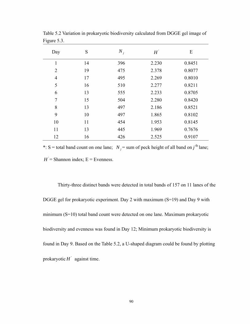
90

Table 5.2 Variation in prokaryotic biodiversity calculated from DGGE gel image of Figure 5.3.

Day S jN 'H E

1 14 396 2.230 0.8451 2 19 475 2.378 0.8077 4 17 495 2.269 0.8010 5 16 510 2.277 0.8211 6 13 555 2.233 0.8705 7 15 504 2.280 0.8420 8 13 497 2.186 0.8521 9 10 497 1.865 0.8102 10 11 454 1.953 0.8145 11 13 445 1.969 0.7676 12 16 426 2.525 0.9107

*: S = total band count on one lane; jN = sum of peck height of all band on j th lane;

'H = Shannon index; E = Evenness.

Thirty-three distinct bands were detected in total bands of 157 on 11 lanes of the

DGGE gel for prokaryotic experiment. Day 2 with maximum (S=19) and Day 9 with

minimum (S=10) total band count were detected on one lane. Maximum prokaryotic

biodiversity and evenness was found in Day 12; Minimum prokaryotic biodiversity is

found in Day 9. Based on the Table 5.2, a U-shaped diagram could be found by plotting

prokaryotic 'H against time.

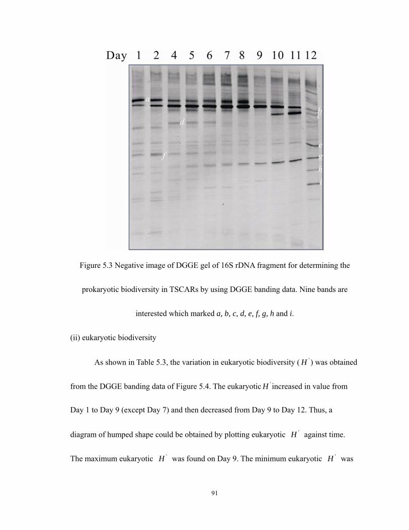
91

Figure 5.3 Negative image of DGGE gel of 16S rDNA fragment for determining the

prokaryotic biodiversity in TSCARs by using DGGE banding data. Nine bands are

interested which marked a, b, c, d, e, f, g, h and i.

(ii) eukaryotic biodiversity

As shown in Table 5.3, the variation in eukaryotic biodiversity ( 'H ) was obtained

from the DGGE banding data of Figure 5.4. The eukaryotic 'H increased in value from

Day 1 to Day 9 (except Day 7) and then decreased from Day 9 to Day 12. Thus, a

diagram of humped shape could be obtained by plotting eukaryotic 'H against time.

The maximum eukaryotic 'H was found on Day 9. The minimum eukaryotic 'H was

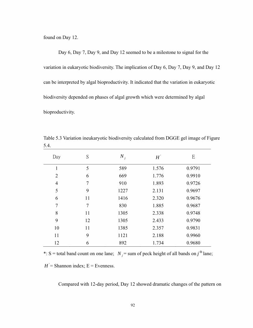
92

found on Day 12.

Day 6, Day 7, Day 9, and Day 12 seemed to be a milestone to signal for the

variation in eukaryotic biodiversity. The implication of Day 6, Day 7, Day 9, and Day 12

can be interpreted by algal bioproductivity. It indicated that the variation in eukaryotic

biodiversity depended on phases of algal growth which were determined by algal

bioproductivity.

Table 5.3 Variation ineukaryotic biodiversity calculated from DGGE gel image of Figure 5.4.

Day S jN 'H E

1 5 589 1.576 0.9791 2 6 669 1.776 0.9910 4 7 910 1.893 0.9726 5 9 1227 2.131 0.9697 6 11 1416 2.320 0.9676 7 7 830 1.885 0.9687 8 11 1305 2.338 0.9748 9 12 1305 2.433 0.9790 10 11 1385 2.357 0.9831 11 9 1121 2.188 0.9960 12 6 892 1.734 0.9680

*: S = total band count on one lane; jN = sum of peck height of all bands on j th lane;

'H = Shannon index; E = Evenness.

Compared with 12-day period, Day 12 showed dramatic changes of the pattern on

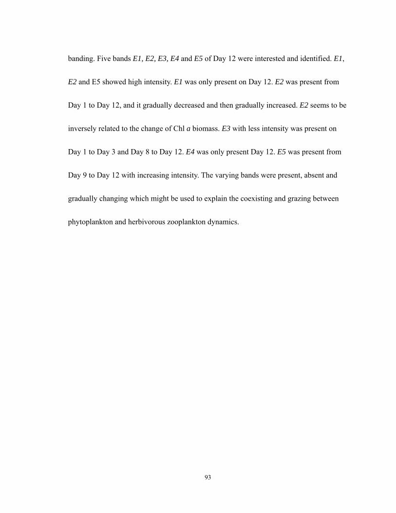
93

banding. Five bands E1, E2, E3, E4 and E5 of Day 12 were interested and identified. E1,

E2 and E5 showed high intensity. E1 was only present on Day 12. E2 was present from

Day 1 to Day 12, and it gradually decreased and then gradually increased. E2 seems to be

inversely related to the change of Chl a biomass. E3 with less intensity was present on

Day 1 to Day 3 and Day 8 to Day 12. E4 was only present Day 12. E5 was present from

Day 9 to Day 12 with increasing intensity. The varying bands were present, absent and

gradually changing which might be used to explain the coexisting and grazing between

phytoplankton and herbivorous zooplankton dynamics.

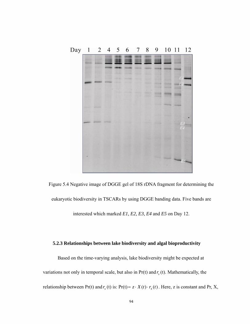
94

Figure 5.4 Negative image of DGGE gel of 18S rDNA fragment for determining the

eukaryotic biodiversity in TSCARs by using DGGE banding data. Five bands are

interested which marked E1, E2, E3, E4 and E5 on Day 12.

5.2.3 Relationships between lake biodiversity and algal bioproductivity

Based on the time-varying analysis, lake biodiversity might be expected at

variations not only in temporal scale, but also in Pr(t) and sr (t). Mathematically, the

relationship between Pr(t) and sr (t) is: Pr(t) )()( trtXz s⋅⋅= . Here, z is constant and Pr, X,

95

and sr are the function of time(t). The lake biodiversity relationships with algal growth

were demonstrated by plotting H’ against Pr(t) and sr (t). As a general trend, the results

showed that when time-varying data were plotted by eukaryotic biodiversity (H’) against

algal bioproductivity, the relationship was hump-shaped, whereas when data were plotted

by prokaryotic biodiversity (H’) against algal bioproductivity, the relationship was

U-shaped.

However, based on time-varying analysis, Day 6, Day 7, Day 9, and Day 12 of

this experiment seemed to be a key point in time which predicted a shift in lake

biodiversity along algal bioproductivity. The implication of Day 6, Day 7, Day 9, and

Day 12 can be interpreted by four algal growth phases separated by sr (t) referred to

Figure 5.2. The Day 6, Day 9 and Day 12 were the demarcation of the four phases: phase

I, phase II, phase III and phase VI, respectively. The interpretation for the critical timing

is: Day 6 displayed the maximum sr ; Day 9 displayed the maximum K; Day 12 reached

the minimum sr ; Day 7 presented the maximum Pr.

Assumption

The concept of the algal growth phase-dependency is proposed to give an

explanation for the varying relationship between between lake biodiversity and algal

bioproductivity. The primary assumptions involved in the explanation of the concept of

96

algal growth phase-dependency control as follow.

(1) It is assumed that algal population is limited in the closed space.

(2) The algal populations are assumed to be growing in the environment with the carrying

capacity (K) due to the available resources such as the limited nutrient phosphorus.

(3) The distribution of species-abundance is a lognormal distribution on the given

microcosm.

(i) the relationships between prokaryotic biodiversity and algal bioproductivity

The relationships between prokaryotic biodiversity (H’) and algal bioproductivity

were demonstrated by plotting prokaryotic biodiversity (H’) versus sr (t) and Pr(t). The

result in the Figure 5.5 sr (t) showed that three varying phases in prokaryotic biodiversity

(H’). During phase I (Day 1 to Day 6), the positive sr (t) was increasing and H’ was

decreasing in a straightforward fashion. When switched to phase II, the positive sr (t)

was decreasing and H’ was also straightforward decreasing during the three days (Day 7

to Day 9). After Day 9, the negative value of sr (t) was increasing and H’ shifted phase II

to phase III with increasing H’value during the three days (Day 10 to Day 12).

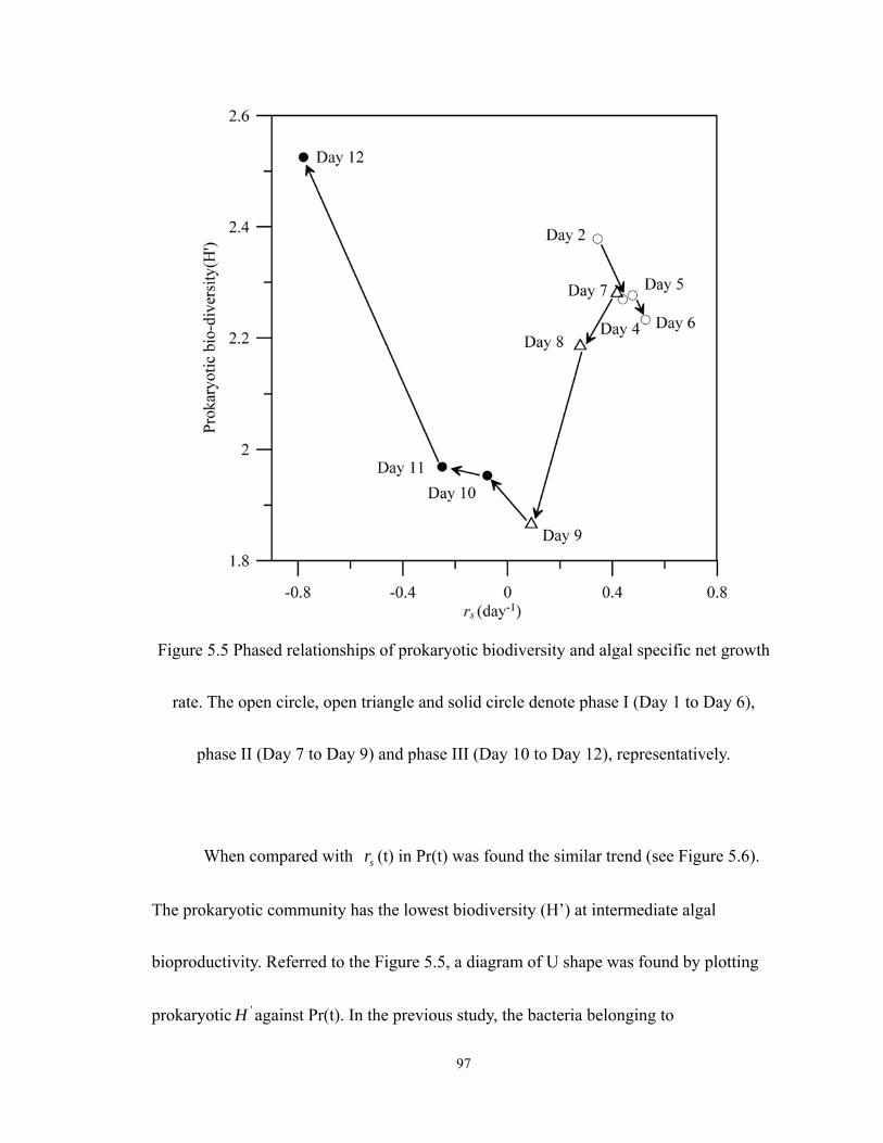
97

Figure 5.5 Phased relationships of prokaryotic biodiversity and algal specific net growth

rate. The open circle, open triangle and solid circle denote phase I (Day 1 to Day 6),

phase II (Day 7 to Day 9) and phase III (Day 10 to Day 12), representatively.

When compared with sr (t) in Pr(t) was found the similar trend (see Figure 5.6).

The prokaryotic community has the lowest biodiversity (H’) at intermediate algal

bioproductivity. Referred to the Figure 5.5, a diagram of U shape was found by plotting

prokaryotic 'H against Pr(t). In the previous study, the bacteria belonging to

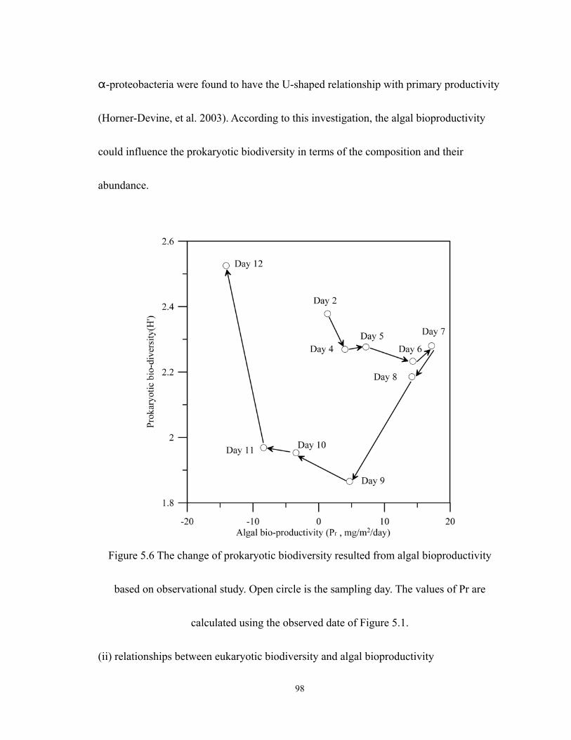
98

"-proteobacteria were found to have the U-shaped relationship with primary productivity

(Horner-Devine, et al. 2003). According to this investigation, the algal bioproductivity

could influence the prokaryotic biodiversity in terms of the composition and their

abundance.

Figure 5.6 The change of prokaryotic biodiversity resulted from algal bioproductivity

based on observational study. Open circle is the sampling day. The values of Pr are

calculated using the observed date of Figure 5.1.

(ii) relationships between eukaryotic biodiversity and algal bioproductivity

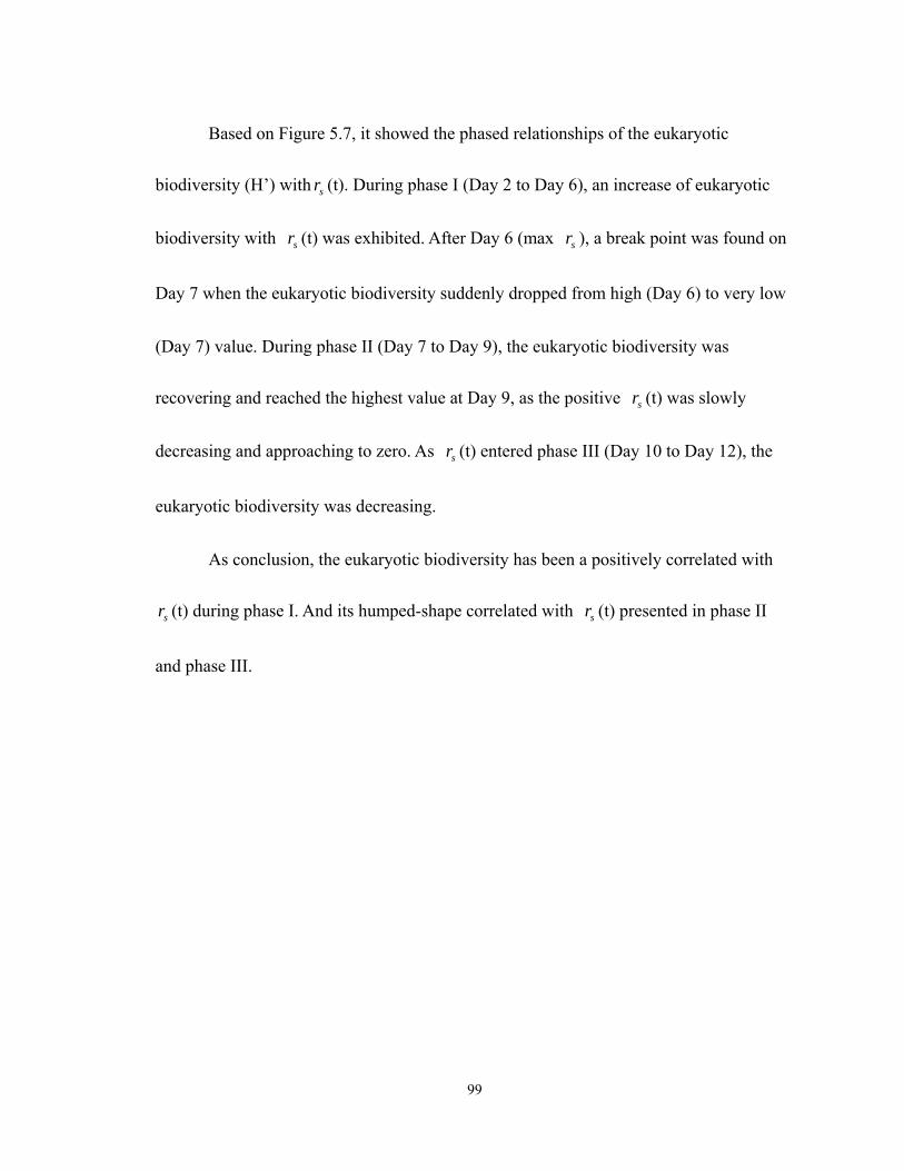
99

Based on Figure 5.7, it showed the phased relationships of the eukaryotic

biodiversity (H’) with sr (t). During phase I (Day 2 to Day 6), an increase of eukaryotic

biodiversity with sr (t) was exhibited. After Day 6 (max sr ), a break point was found on

Day 7 when the eukaryotic biodiversity suddenly dropped from high (Day 6) to very low

(Day 7) value. During phase II (Day 7 to Day 9), the eukaryotic biodiversity was

recovering and reached the highest value at Day 9, as the positive sr (t) was slowly

decreasing and approaching to zero. As sr (t) entered phase III (Day 10 to Day 12), the

eukaryotic biodiversity was decreasing.

As conclusion, the eukaryotic biodiversity has been a positively correlated with

sr (t) during phase I. And its humped-shape correlated with sr (t) presented in phase II

and phase III.

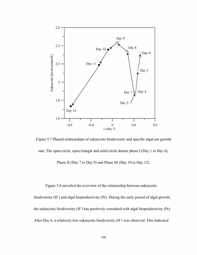
100

Figure 5.7 Phased relationships of eukaryotic biodiversity and specific algal net growth

rate. The open circle, open triangle and solid circle denote phase I (Day 1 to Day 6),

Phase II (Day 7 to Day 9) and Phase III (Day 10 to Day 12).

Figure 5.8 unveiled the overview of the relationship between eukaryotic

biodiversity (H’) and algal bioproductivity (Pr). During the early period of algal growth,

the eukaryotic biodiversity (H’) has positively correlated with algal bioproductivity (Pr).

After Day 6, a relatively low eukaryotic biodiversity (H’) was observed. This indicated

101

that eukaryotic biodiversity (H’) has a break point when Pr reached maximum value.

During the period of Day 7 to Day 12, humped-shape relationship between H’ and Pr was

formed. As Pr was approaching to zero, the peak of eukaryotic biodiversity (H’) occurred.

Figure 5.8 The act of changing eukaryotic biodiversity resulted from algal

bioproductivity based on observational study. Open circle is the sampled day. The values

of Pr are calculated using the observed date of Figure 5.1 referred to the procedure of Pr

estimation in Chapter 3.

102

5.3 Discussion

The development of algal phytoplankton community is a dynamic process. The

many physical and biological mechanisms could potentially influence the patterns of

biodiversity-bioproductivity in the algal phytoplankton community. The factors correlated

with biodiversity are the basis in understanding how biodiversity is regulated.

Algal population dynamics of CSTR system can be expressed by algal net growth

rate ( sr ).The algal net growth rate ( sr ) can increase and decrease due to the algal gross

growth rate ( gµ ) and algal loss rate ( lλ ). In the CSTR system the algal populations are

introduced and incubated under an environment where nutrients and physical conditions

are kept consistent. A situation is the fact that the algal population dynamics can be

affected by its population size, environmental resistance and the biological factor of other

populations. The concept of algal population dynamics is essential for describing algal

growth rate, related interaction and regulation among the populations during growth

phases. Depending on the algal bioproductivity, algal population dynamics correlates

closely with the algal net growth rate. The algal growth can be expressed as the algal

growth under unlimited conditions, following the potential environmental resistance, and

then the negative growth rate caused by other species interactions. The concept of

considering a population growth rate depending on population size is used to express the

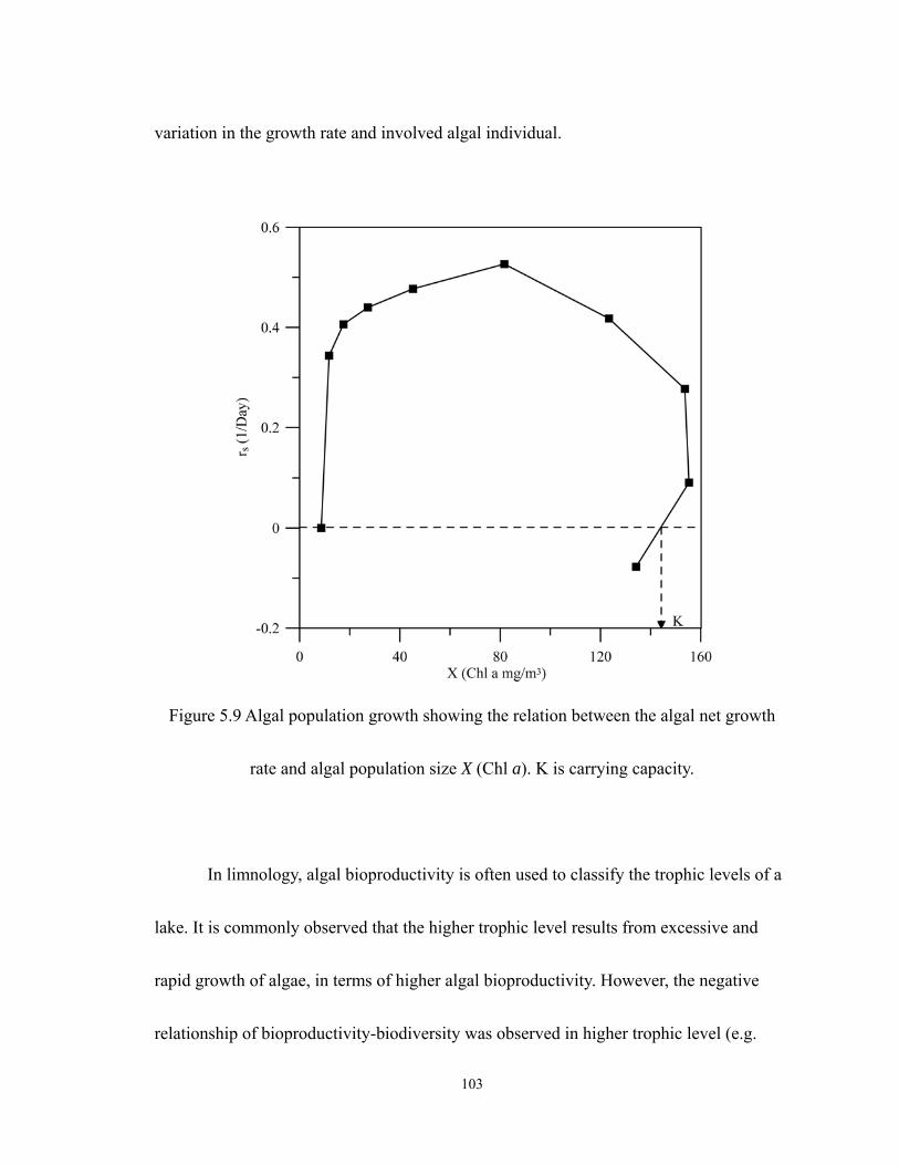
103

variation in the growth rate and involved algal individual.

Figure 5.9 Algal population growth showing the relation between the algal net growth

rate and algal population size X (Chl a). K is carrying capacity.

In limnology, algal bioproductivity is often used to classify the trophic levels of a

lake. It is commonly observed that the higher trophic level results from excessive and

rapid growth of algae, in terms of higher algal bioproductivity. However, the negative

relationship of bioproductivity-biodiversity was observed in higher trophic level (e.g.

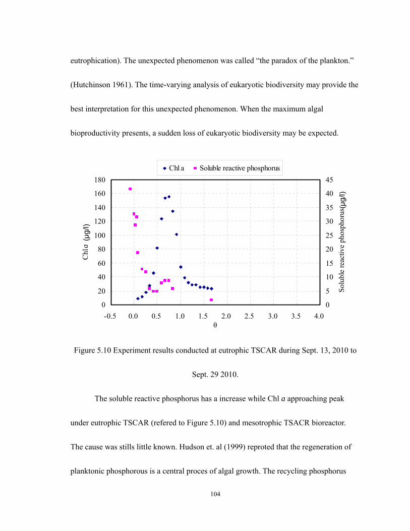
104

eutrophication). The unexpected phenomenon was called “the paradox of the plankton.”

(Hutchinson 1961). The time-varying analysis of eukaryotic biodiversity may provide the

best interpretation for this unexpected phenomenon. When the maximum algal

bioproductivity presents, a sudden loss of eukaryotic biodiversity may be expected.

0

20

40

60

80

100

120

140

160

180

-0.5 0.0 0.5 1.0 1.5 2.0 2.5 3.0 3.5 4.0θ

Chl

a (μ

g/l)

0

5

10

15

20

25

30

35

40

45

Solu

ble

reac

tive

phos

phor

us (μ

g/l)

Chl a Soluble reactive phosphorus

Figure 5.10 Experiment results conducted at eutrophic TSCAR during Sept. 13, 2010 to

Sept. 29 2010.

The soluble reactive phosphorus has a increase while Chl a approaching peak

under eutrophic TSCAR (refered to Figure 5.10) and mesotrophic TSACR bioreactor.

The cause was stills little known. Hudson et. al (1999) reproted that the regeneration of

planktonic phosphorous is a central proces of algal growth. The recycling phosphorus

105

supplied the major nutrient for primary productivity. Figure 5.10 showed that it may have

resulted in the regeneration of phosphorus. It suggests that huge population may be

digested and then released phosphorus. It could be evidence to describe how the lake

biodiversity presents huge losses before reaching peak biomass.

106

CHAPTER 6. MOLECULAR PHYLOGENY OF EUKARYOTIC

ASSEMBLAGE UNDER VARYING TROPHIC LEVELS

The eukaryotic biodiversity was examined by molecular cloning and sequencing

the 18S ribosomal DNA in three bioreactors differing by their trophic levels (oligotrophic,

mesotrophic, and eutrophic levels). The results of sequence analysis showed that the

composition of the eukaryotic community and lineages were subjected to the lake trophic

status. The Ek4 library reflected higher equitability than EK5 and EK6 by used Shannon

evenness, in other words, lower clone dominance was observed in the oligotrophic

assemblage survey. The Shannon index of Ek5 appeared more diverse than Ek4 and Ek6.

The discovery of unknown species and new phylogentic groups identified were found in

PK6, EK4, EK5, and EK6 libraries.

6.1 Results

The results of the clone library provided the informative phylogeny

characterization of eukaryotic and prokaryotic assemblage (Lopez-Garcia,

Rodriguez-Valera, et al. 2001; Moon-van der Staay, De Wachter, et al. 2001). Each library

(Ek4, Ek5 and Ek6) randomly picked up approximately 63 positive clones, except for

Pk6 library samples where only 37 positive clones were analyzed. For prokaryotes, the

Pk6 library constructed was analyzed, producing 10 different operational taxonomic units

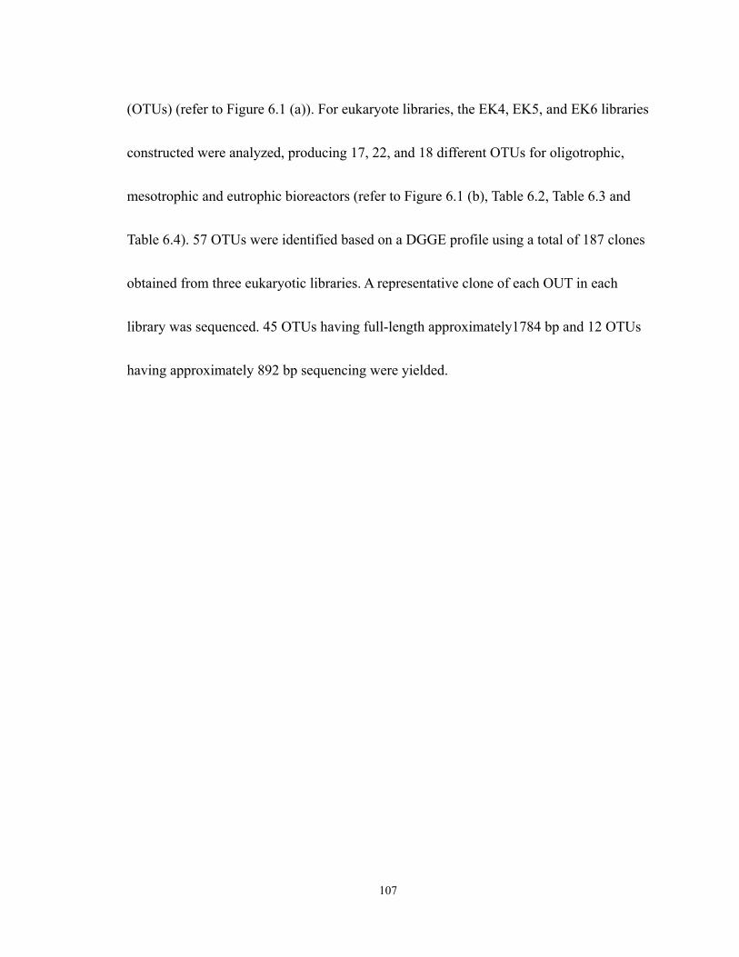
107

(OTUs) (refer to Figure 6.1 (a)). For eukaryote libraries, the EK4, EK5, and EK6 libraries

constructed were analyzed, producing 17, 22, and 18 different OTUs for oligotrophic,

mesotrophic and eutrophic bioreactors (refer to Figure 6.1 (b), Table 6.2, Table 6.3 and

Table 6.4). 57 OTUs were identified based on a DGGE profile using a total of 187 clones

obtained from three eukaryotic libraries. A representative clone of each OUT in each

library was sequenced. 45 OTUs having full-length approximately1784 bp and 12 OTUs

having approximately 892 bp sequencing were yielded.

108

(a) (b)

Figure 6.1 DGGE profile image of prokaryotic and eukaryotic cloning libraries termed

Pk6, Ek4, Ek5, and Ek6 with representative clones. (a) Comparison of DGGE profile of

the eutrophic bioreactor mixed community to prokaryotic clones containing insert 16S

rDNA gene. Lane1, eutrophic bioreactor mixed community; Lane2, EP 3; Lane3, EP 5;

Lane4, EP 13; Lane5, EP 15; Lane6, EP 16; Lane7, EP 18; Lane8, EP 19; Lane9, EP 29;

Lane10, EP 30; Lane11, EP 61; Lane12, EP 62. (b) DGGE image demonstrates that the

DGGE banding data depicted the OTUs of each eukaryotic libraries (lane1 :Ek4,

lane2 :Ek5, and lane3: Ek6)

109

6.1.1 Eukaryotic libraries in TSCARs

The overall composition of the eukaryotic community often was interpreted by

species richness (number of species), abundance (number of individuals) and evenness

(level of dominance) in classical ecological biodiversity studies (MacArthur and Wilson

1967; May 1975, Pielou 1975). Contemporary studies on eukaryotic biodiversity based

on the method of sequencing 18S rDNA were often used for analyzing the composition of

the community and the OTUs were regarded as the surrogates of taxa or species (Bent

and Forney 2008; Curtis, Head, et al. 2006). Indeed, the method allowed for an improved

understanding of the common and rare species in lake biodiversity, especially the

discovery of unknown species and new phylogentic groups (Lefèvre, Bardot, et al. 2007;

Richards, Vepritskiy, et al. 2005).

In this clone library study, the raw data (plotted Figure 6.2) shows the relationship

between species richness and relative abundance in three clone libraries (Ek4, Ek5, and

Ek6). The plots provided information on a number of species and on their relative

abundance as well as the potential dominance species. Figure6.2 illustrates that in the

data sets it was found that a few species were particularly abundant, such as Ek4.16,

Ek5.1 and Ek6.9, some species of varying intermediate degree, while most of the species

appeared as a few individuals.

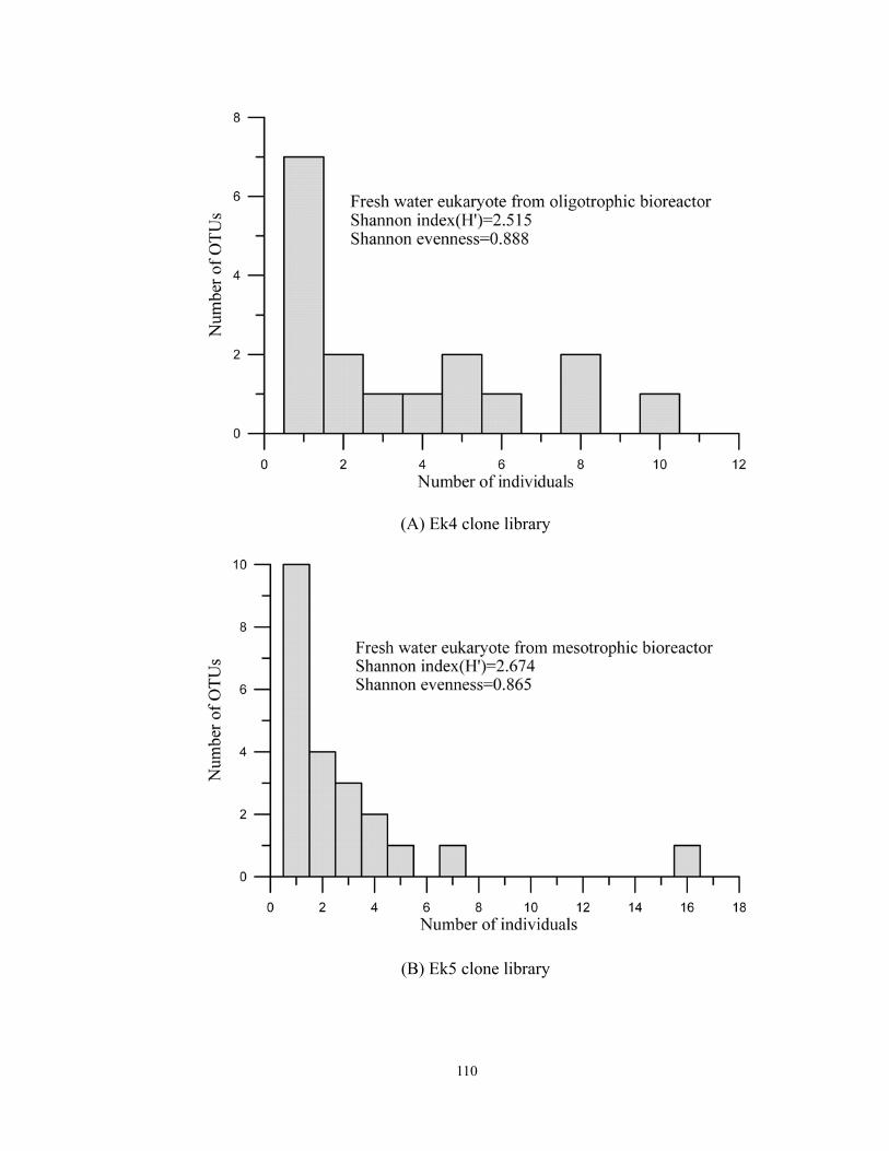
110

(A) Ek4 clone library

(B) Ek5 clone library

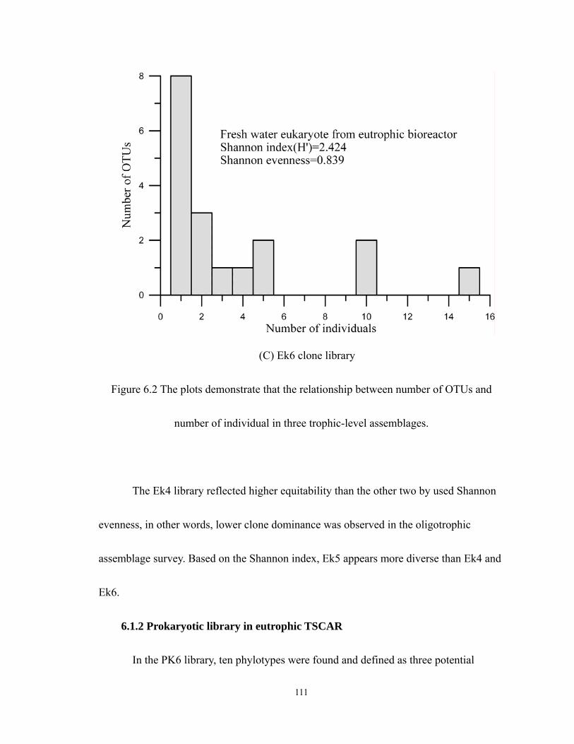
111

(C) Ek6 clone library

Figure 6.2 The plots demonstrate that the relationship between number of OTUs and

number of individual in three trophic-level assemblages.

The Ek4 library reflected higher equitability than the other two by used Shannon

evenness, in other words, lower clone dominance was observed in the oligotrophic

assemblage survey. Based on the Shannon index, Ek5 appears more diverse than Ek4 and

Ek6.

6.1.2 Prokaryotic library in eutrophic TSCAR

In the PK6 library, ten phylotypes were found and defined as three potential

112

groups: Proteobacteria, Cyanobacteria, and unidentified environmental samples (see

Table 6.1). The bacterial communities in lakes play a central role and obtained more

attention in lake field investigations. Van et al. reported that the groups (such as

Actinobacteria, Betaproteobacteria, Bacteroidetes, and Cyanobacteria ) of bacterial

communities in freshwater lakes related to the food-wed variation.(Van der Gucht,

Vandekerckhove, et al. 2005). The Cyanobacteria bloom obtained more attention among

those function groups (Eiler and Bertilsson 2004) due to water quality issues. Limited in

data of sequence demonstrated of the PK6 were merely preliminary in the community

structure analysis. Based on the sequencing data, PK6 was dominated by EP5. In

environmental sample group, fourteen positive clones clustered with EP5 with 95%

similarity related to uncultured bacterium clone A5-083. The high percentage of

unidentified environmental samples occupied PK6. It pointed out that additional

investigation of prokaryotic biodiversity are necessary.

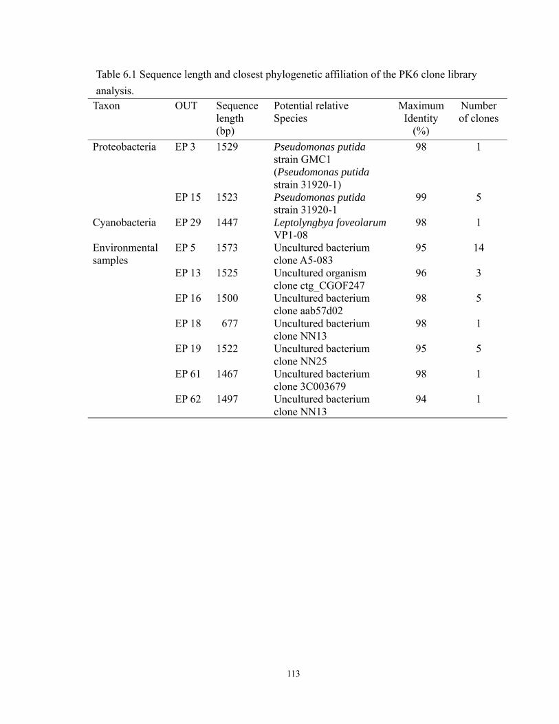
113

Table 6.1 Sequence length and closest phylogenetic affiliation of the PK6 clone library analysis.

Taxon OUT Sequence length (bp)

Potential relative Species

Maximum Identity

(%)

Number of clones

Proteobacteria EP 3 1529 Pseudomonas putida strain GMC1 (Pseudomonas putida strain 31920-1)

98 1

EP 15 1523 Pseudomonas putida strain 31920-1

99 5

Cyanobacteria EP 29 1447 Leptolyngbya foveolarum VP1-08

98 1

Environmental samples

EP 5 1573 Uncultured bacterium clone A5-083

95 14

EP 13 1525 Uncultured organism clone ctg_CGOF247

96 3

EP 16 1500 Uncultured bacterium clone aab57d02

98 5

EP 18 677 Uncultured bacterium clone NN13

98 1


95 5

EP 61 1467 Uncultured bacterium clone 3C003679

98 1


94 1

114

6.2 Phylogenetic analyses

A total of fifty-seven insert 18S rDNA consisting of forty-six completely and

eleven partially sequences were used in the phylogenetic analyses for all three libraries

EK4, EK5 and EK6.

EK4 cloning library

In the EK4 library, seventeen phylotypes were found and defined as ten

phylogenetic groups: Chlorophyta, Heterolobosea, Cryptophyta, Stramenopiles, Cercozoa,

Fungi, Rotifera, Amoebozoa, Alveolata and unidentified eukaryote (Table 6.2). In several

field investigations, these phyla were often present in oligotrophic lakes (Lefranc, et al.

2005; Richards, et al. 2005). According to analysis, two main phyla, Chlorophyta (27%)

and Stramenopiles (25%) were clearly observed in the EK4 library. In Chlorophyta group,

thirteen positive clones clustered with EK4.14 and EK4.5 with 97% similarity related to

Coccomyxa sp. and four clones belonging to EK4.1 with 98% similarity related to

Botryococcus braunii. The Botryococcus braunii (4 clones) and Coccomyxa sp. (13

clones) are detected in the EK4 library. Both of the two nonmotile greens are

characteristic of oligotrophic lakes. The Botryococcus braunii was found frequently in

lakes of low productivity (Huszar, Kruk, et al. 2003; Wake and Hillen 1981) and low

saline waters (Davis, Kolva, et al. 1977).

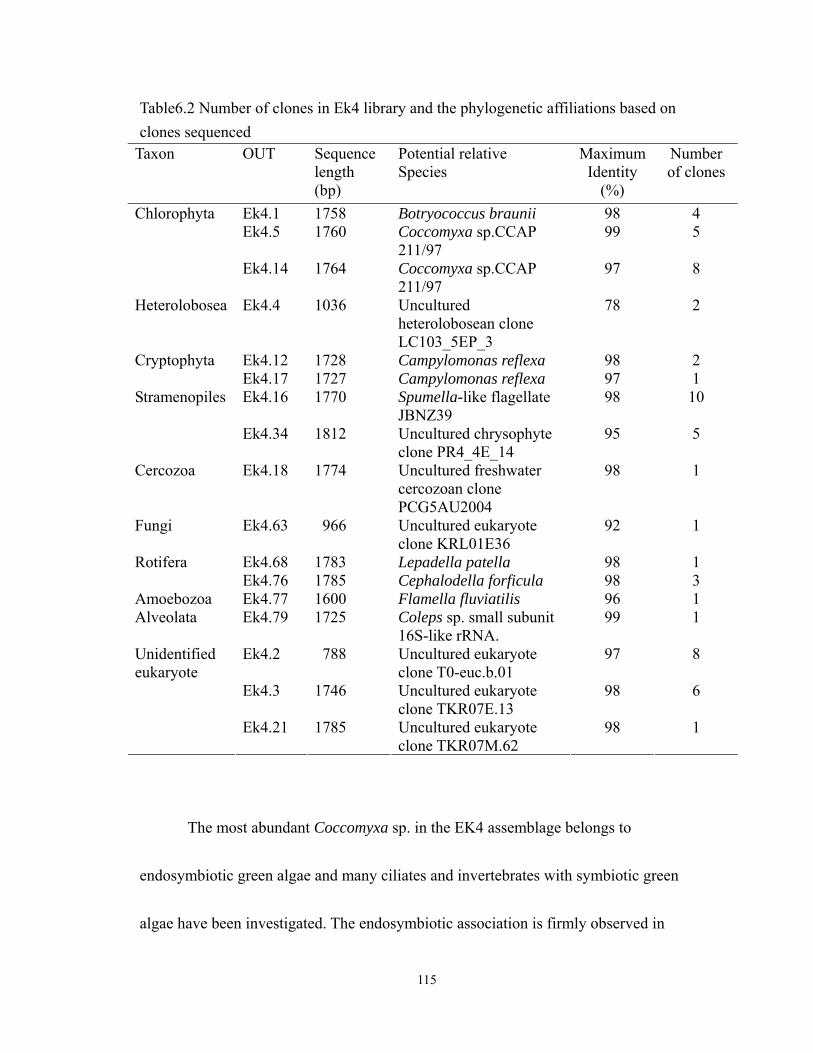
115

Table6.2 Number of clones in Ek4 library and the phylogenetic affiliations based on clones sequenced


Potential relative Species

Maximum Identity

(%)

Number of clones

Chlorophyta Ek4.1 1758 Botryococcus braunii 98 4 Ek4.5 1760 Coccomyxa sp.CCAP

211/97 99 5

Ek4.14 1764 Coccomyxa sp.CCAP 211/97

97 8

Heterolobosea Ek4.4 1036 Uncultured heterolobosean clone LC103_5EP_3

78 2

Cryptophyta Ek4.12 1728 Campylomonas reflexa 98 2 Ek4.17 1727 Campylomonas reflexa 97 1 Stramenopiles Ek4.16 1770 Spumella-like flagellate

JBNZ39 98 10

Ek4.34 1812 Uncultured chrysophyte clone PR4_4E_14

95 5

Cercozoa Ek4.18 1774 Uncultured freshwater cercozoan clone PCG5AU2004

98 1

Fungi Ek4.63 966 Uncultured eukaryote clone KRL01E36

92 1

Rotifera Ek4.68 1783 Lepadella patella 98 1 Ek4.76 1785 Cephalodella forficula 98 3 Amoebozoa Ek4.77 1600 Flamella fluviatilis 96 1 Alveolata Ek4.79 1725 Coleps sp. small subunit

16S-like rRNA. 99 1

Ek4.2 788 Uncultured eukaryote clone T0-euc.b.01

97 8

Ek4.3 1746 Uncultured eukaryote clone TKR07E.13

98 6

Unidentified eukaryote

Ek4.21 1785 Uncultured eukaryote clone TKR07M.62

98 1

The most abundant Coccomyxa sp. in the EK4 assemblage belongs to

endosymbiotic green algae and many ciliates and invertebrates with symbiotic green

algae have been investigated. The endosymbiotic association is firmly observed in

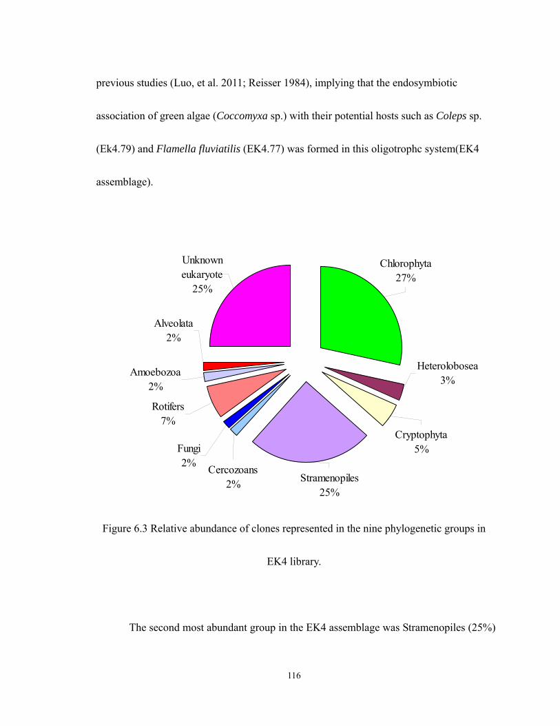
116

previous studies (Luo, et al. 2011; Reisser 1984), implying that the endosymbiotic

association of green algae (Coccomyxa sp.) with their potential hosts such as Coleps sp.

(Ek4.79) and Flamella fluviatilis (EK4.77) was formed in this oligotrophc system(EK4

assemblage).

Amoebozoa2%

Stramenopiles25%

Chlorophyta27%

Cryptophyta5%

Heterolobosea3%

Rotifers7%

Alveolata2%

Fungi2% Cercozoans

2%

Unknowneukaryote

25%

Figure 6.3 Relative abundance of clones represented in the nine phylogenetic groups in

EK4 library.

The second most abundant group in the EK4 assemblage was Stramenopiles (25%)

117

with ten of clones. This group was related to Spumella-like flagellate (Ek4.16) with 98%

similarity. Five of the clones were found close to the uncultured chrysophyte clone

PR4_4E_14 with 95% similarity OUT (EK4.34). Lara et al.(2011) reported that the

sequence of PR4_4E_14 is associated with Spumella-like flagellate (Lara, Mitchell, et al.

2011). The Spumella-like flagellate belonging to colorless, heterotrophic nanoflagellate

(HNF), plays important role in carbon transfer and nutrient regeneration of aquatic food

webs. However, the unexpected diversity was only recently investigated. Boenigk et

al.(2005) reported that the Spumella of HNF are a high diverse group and commonly

found in different geographic regions (Boenigk, Pfandl, et al. 2005). Several field

investigations indicated that this function group, comprised of HNF, bacteria and ciliates,

is associateed with lake productivity (Auer and Arndt 2001).

The Cryptophyta were detected two OTUs (EK12 and EK17), belonging to

Campylomonas reflexa, one of primary producers, from EK4 assemblage which occupied

5% of clonal abundance. The lower proportion of clonal abundance are also found in

recently lake and coastal studies, for instance, 7% of clonal abundance was observed in

Lake Godivelle (Lefranc, et al. 2005), 10% in Lake Fuschlsee (Medinger, Nolte, et al.

2010), and 4% in Blanes Bay (Massana, Balagué, et al. 2004). In spite of the limitation in

evidence found in the observation, the results suggested that the lower abundance of

118

Cryptophyta may associate with the trophic status in lakes. Auer (2001) indicated that the

Cryptophyta group are positively correlated with lake bioproductivity in field

investigation by non-molecular analysis (Auer and Arndt 2001).

Alveolate is a super phylum comprising ciliates, dinoflagellates, the parasitic

apicomplexa and perkinsozoa (Moreira and Lpóez-Garca 2002). In this EK4 assemblage,

they are represented by one OUT (EK4.79) associated with heterotrophic ciliophora:

Coleps sp.. Field investigations indicated that Coleps sp. was the low grazing rates of

detritofagous species (Sanders, Porter, et al. 1989; Simek, Bobkova, et al. 1995).

Although EK4.79 was relatively low in abundance (2%), the Coleps sp. of heterotrophic

ciliates plays an important role in parasites of green algae.

Two OTUs were grouped within the Rotifera which was regarded as a significant

consumer of bacteria in freshwaters. EK4.68 and EK4.76 obtained 98% similarity with

Lepadella patella and Cephalodella forficula, respectively. Both were found in an

oligotrophic lake(Casper, Flobner, et al. 1985).

Three unidentified OTUs (Ek4.2, Ek4.3 and Ek4.21) were found in the EK4

library. Ek4.2, Ek4.3 and Ek4.21 belonged to environmental samples: uncultured

eukaryote clone T0-euc.b.01, uncultured eukaryote clone TKR07E.13 and uncultured

eukaryote clone TKR07M.62 with 97%, 98%, and 98% similarity, respectively. The two

119

sequences (uncultured eukaryote clone TKR07E.13 and uncultured eukaryote clone

TKR07M.62) were originally detected in the oligotrophic Lake Tanganyika (Tarbe,

Stenuite, et al. 2011).

Based on the species abundance distribution (referred to Figure 6.2(a)), the three

OTUs (EK4.14, EK4.16 and EK4.2) affiliated with Coccomyxa sp., Spumella-like

flagellate and unidentified eukaryote (EK4.2) were recognized as the certain members of

the EK4 library. The six OTUs (Ek4.1, Ek4.4, Ek4.12, Ek4.34, Ek4.76 and Ek4.3) are

arranged in the moderately relative common groups, including Botryococcus braunii,

uncultured heterolobosean clone LC103_5EP_3, Campylomonas reflexa, uncultured

chrysophyte clone PR4_4E_14, Cephalodella forficula, unidentified eukaryote (EK4.3).

Rare species were classified as those represented by single number of OUTs in taxon

groups. Approximately 41% of OTUs (7 species observed) is rare in the EK4 library.

EK5 cloning library

The composition of a eukaryotic assemblage in a mesotrophic bioreactor (EK5

library) was investigated showing nine different phylogenetic groups: Chlorophyta,

Heterolobosea, Cryptophyta, Stramenopiles, Cercozoa, Fungi, Metazoans, Alveolata, and

LKM11 (Referred toTable 6.3). The dominant group was the Cryptophyta group which

occupied 26% of clonal abundance observed in the EK5 cloning library. The Chlorophyta,

120

Fungi and LKM11 groups occupied 17%, 17% and 14% of clonal abundance,

respectively. The five other groups: Heterolobosea, Stramenopiles, Cercozoa, Metazoans,

and Alveolata obtained less then 10% of clonal abundance (see Figure 6.4).

In Cryptophyta group, sixteen positive clones clustered with EK5.1 obtained 97%

similarity with Campylomonas reflexa, a most abundant individual in the EK5 library.

Campylomonas reflexa is often found in diversely trophic-level lakes (Muller Ogle,

Peterson, et al. 1999). Cryptophyta grown in light-limited and ice-covered lakes have

been observed in field investigations (Pasztaleniec and Lenard 2008; Phillips and Fawley

2002). The Chlorophyta group occupied 17% of relative abundance in the EK5 library is

also well presented. Seven OTUs were detected including Makinoella tosaensis,

Botryococcus braunii, Coccomyxa sp.CCAP 211/97, Scenedesmus regularis,

Kirchneriella obesa strain ACOI 3125, Botryococcus braunii and uncultured eukaryote

clone KRL01E41 with more then 94% similarity. The proportions of Chlorophyta are

highest among the three trophic-level libraries, contributing to 32% of OTUs in EK5. It

suggests that the highest species richness of Chlorophyta represented in the mesotrophic

lake. Compared with EK4 library, the Chlorophyta increased in number of species, but

decreased in number of individuals in the EK5 library.

121

Table6.3 Number of clones in EK5 library and the phylogenetic affiliations based on clones sequenced


Potential relative species

Maximum Identity

(%)

Number of

clones Chlorophyta Ek5.3 1749 Makinoella tosaensis 94 1 Ek5.16 1758 Botryococcus braunii 98 1 Ek5.33 1760 Coccomyxa sp.CCAP

211/97 99 2

Ek5.90 1735 Scenedesmus regularis 94 2 Ek5.127 1756 Kirchneriella obesa strain

ACOI 3125 97 1

Ek5.65 969 Botryococcus braunii 1 Ek5.7 1749 Uncultured eukaryote

clone KRL01E41 96 3


83 5

Cryptophyta Ek5.1 1727 Campylomonas reflexa 97 16 Stramenopiles Ek5.85 1629 Spumella sp. TGS6 99 3 Cercozoa Ek5.39 1050 Lecythium sp. 95 1 Ek5.70 1774 Uncultured freshwater

cercozoan clone PCG5AU2004

98 2

Ek5.82 1672 Uncultured freshwater cercozoan clone PCH11AU2004

97 2

Fungi Ek5.26 926 Uncultured fungus clone D53

98 3

Ek5.71 966 Uncultured eukaryote clone KRL01E36

92 4

Ek5.31 1750 Uncultured eukaryote clone PF7AU2004

99 4

Metazoans Ek5.122 699 Capsaspora owczarzaki 95 1 Alveolata Ek5.80 1724 Uncultured ciliate clone

AY2009C19 98 1

Ek5.130 1707 Coleps hirtus 98 1 Ek5.27 1750 Uncultured eukaryotic

picoplankton clone P34.42 94 7

Ek5.78 732 Uncultured eukaryotic picoplankton clone P34.42

97 1

Unidentified eukaryote (LKM11)

Ek5.116 1716 Uncultured eukaryotic picoplankton clone P34.42

94 1

122

According to the literature, the field investigations of mesotrophic lake showed

that the proportion of Chlorophyta represent 17.9% of total eukaryoyic assemblage

(Mangot, et al. 2009).

The fungi group of Ek5 occupied 17% of clones, which formed three different

OTUs (EK5.26, EK5.71, and EK5.31) which is similar to the result (11.4%) conducted by

Mangot, Lepère et al. (2009). Three clones of EK5.26 were related to clone D53 with

98% similarity; four clones of EK5.71 were traced to uncultured eukaryote clone

KRL01E36 based on 94% similarity. Moreover, four clones of EK5.31 was closely linked

to uncultured eukaryote clone PF7AU2004 with 98% similarity affiliated with zoosporic

fungi based on the investigation in Lake Pavin (Lefèvre, Jobard, et al. 2010). Compared

with EK5.26, the highly similar observation of clone PFD5AU2004 clustered to novel

clade of fungi with 98% similarity was made (Lefèvre, et al. 2007) and Lefèvre et

al.(2007) highlighted that fungal zooflagellates are important member of the functional

groups in oligomesotrophic Lake Pavin. The three unknown sequences could not have

been identified as species level of fungi based on current data, because they are limited

by the lack of species descriptions. These small fungi (<5:m) are recognized as important

members in lake systems (Lefèvre, et al. 2007), since the function groups are considered

to be parasites of the phytoplankton (Kagami, Donk, et al. 2004; Lepère, Domaizon, et al.

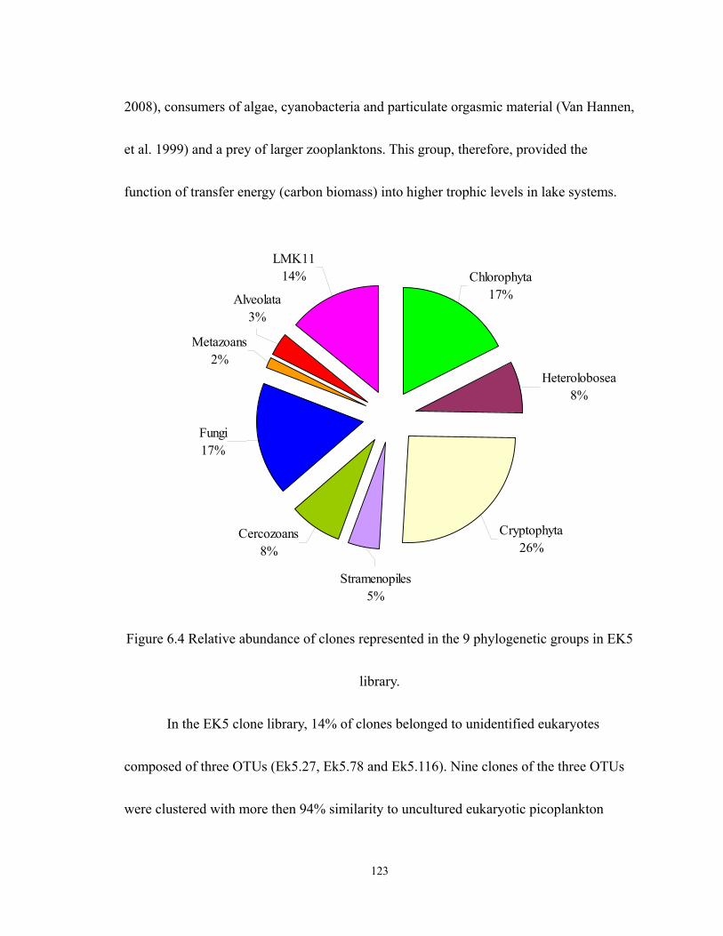
123

2008), consumers of algae, cyanobacteria and particulate orgasmic material (Van Hannen,

et al. 1999) and a prey of larger zooplanktons. This group, therefore, provided the

function of transfer energy (carbon biomass) into higher trophic levels in lake systems.

Fungi17%

Cryptophyta26%

Heterolobosea8%

Stramenopiles5%

Cercozoans8%

Metazoans2%

Alveolata3%

LMK1114% Chlorophyta

17%

Figure 6.4 Relative abundance of clones represented in the 9 phylogenetic groups in EK5

library.

In the EK5 clone library, 14% of clones belonged to unidentified eukaryotes

composed of three OTUs (Ek5.27, Ek5.78 and Ek5.116). Nine clones of the three OTUs

were clustered with more then 94% similarity to uncultured eukaryotic picoplankton

124

clone P34.42 detected in oligomesotrophic Lake Pavin (Lefranc, et al. 2005). The P34.42

was affiliated with the clade LMK11 defined by Van Hannen et al. (Van Hannen, et al.

1999). Mangot, Lepère et al. (2009) reported that the LMK11 found 4.5% of clones

relative abundance in the mesotrophic Lake Bourget (Mangot, et al. 2009). According to

phylogenetic analysis (Van Hannen, et al. 1999), LMK11 group is regarded as a novel

cluster and is strongly associated with Fungi. LMK11 is often found in the oligotrophic

and mesotrophic lakes (Lefranc, et al. 2005; Lepère, et al. 2006; Lepère, et al. 2008;

Mangot, et al. 2009).

Three OTUs (Ek5.39, Ek5.70 and Ek5.82) were grouped within Cercozoa phylum

with more then 95% similarity. The sequence of EK5.39 linked to the core cercozoa:

Lecythium sp., a small (5-10:m in size) heterotrophic filose amoeba known as a bacterial

feeder (Nikolaev, Berney, et al. 2003). The EK5.70 and EK5.82 are closely related to

uncultured freshwater cercozoan clone PCG5AU2004 and uncultured freshwater

cercozoan clone PCH11AU2004 belonged to novel clade II of Cercozoa. The two

sequences of novel clade II were firstly defined by Lefevre et al. (2007) based on the

investigation of HF in Lake Pavin (Lefèvre, et al. 2007). EK5.25 obtained 8% of the

clones abundance and belonged to the Heterolobosea phylum. The sequence of EK5.25

were related to the sequence of clone LC103_5EP_3 with lower similarity (83%)

125

identified by López-García et al. (López-García, Vereshchaka, et al. 2007).

The population of Stramenopiles (5%), Metazoans (2%) and Alveolata (3%) in

EK5 library is rare. Three clones were detected belonging to Ek5.85 grouped into

Stramenopiles and traced to Spumella sp. TGS6 with 99% similarity. In the previous

studies, the heterotrophic spumella of small Chrysophyceae were common observed in

freshwaters, but spumella-like flagellates did not dominate the mesotrophic lakes

(Lefranc, et al. 2005; Lepère, et al. 2006).

Two OTUs (Ek5.80 and Ek130) were clustered into Alveolata (3% of clones).

Ek5.80 had 98% similarity to uncultured ciliate clone AY2009C19 first identified by

Monchy et al.(2011) in Lake Aydat (Monchy, Sanciu, et al. 2011). The sequence of

Ek5.130 was related to Coleps hirtus hirtus based on 98% similarity. Barth, et al. (2008)

reported that the Coleps hirtus hirtus was found only in autumn based on the samples of

Coleps isolated from mesotrophic reservoir Saidenbach (Germany) (Barth, Tischer, et al.

2008).

EK6 cloning library

According to the phylogenetic analysis, eight groups: Chlorophyta, Heterolobosea,

Cryptophyta, Stramenopiles, Apusozoa, Fungi, Alveolata, and uncultured eukaryote, were

detected in the EK6 cloning library, which are commonly found in eutrophic lakes

126

(Huszar, et al. 2003; Lefranc, et al. 2005; Nixdorf, Mischke, et al. 2003). The diagram

(Figure 6.6) shows one major phylum, Cryptophyta (48% of clone abundance) in the EK6

library. The Apusozoa and Chlorophyta are well represented, according for16% and 10%

of clone abundance, respectively. Anther five groups: Heterolobosea, Stramenopiles,

Fungi, Alveolata, and uncultured eukaryote are less then 8% of clone abundance.

Among the taxa groups, the EK6 library was clearly dominated by Cryptophyta

group occupied 48% of clone abundance. Cryptophyta phylum of EK6 cloning library

comprises two subgroups: Cryptomonadales (EK6.9 and EK6.35) and Pyrenomonadales

(EK6.38). Fifteen clones belonged to EK6.9 with 96% similarity related to Cryptomonas

marssonii strain WCK01 identified by Kim et al. (Kim, Boo, et al. 2007); four clones of

EK6.35 exhibited 98% similarity to Campylomonas reflexa; ten clones of EK6.38 are

close to Komma caudate based on 98% similarity. The morphological features between

Cryptomonas marssonii and Campylomonas reflexa is very similar based on Hill’s

description (Hill 1991). However, the main distinguish between the two is the pyrenoid, a

center of carbon dioxide fixation, that is, Campylomonas reflexa possesses pyrenoids, but

Cryptomonas marssonii does not (Hill 1991; Javornicky 2003). Recently, based on

molecular technology more novel species and its diversity are discovered (Marin,

Klingberg, et al. 1998; Metfies, Gescher, et al. 2010).

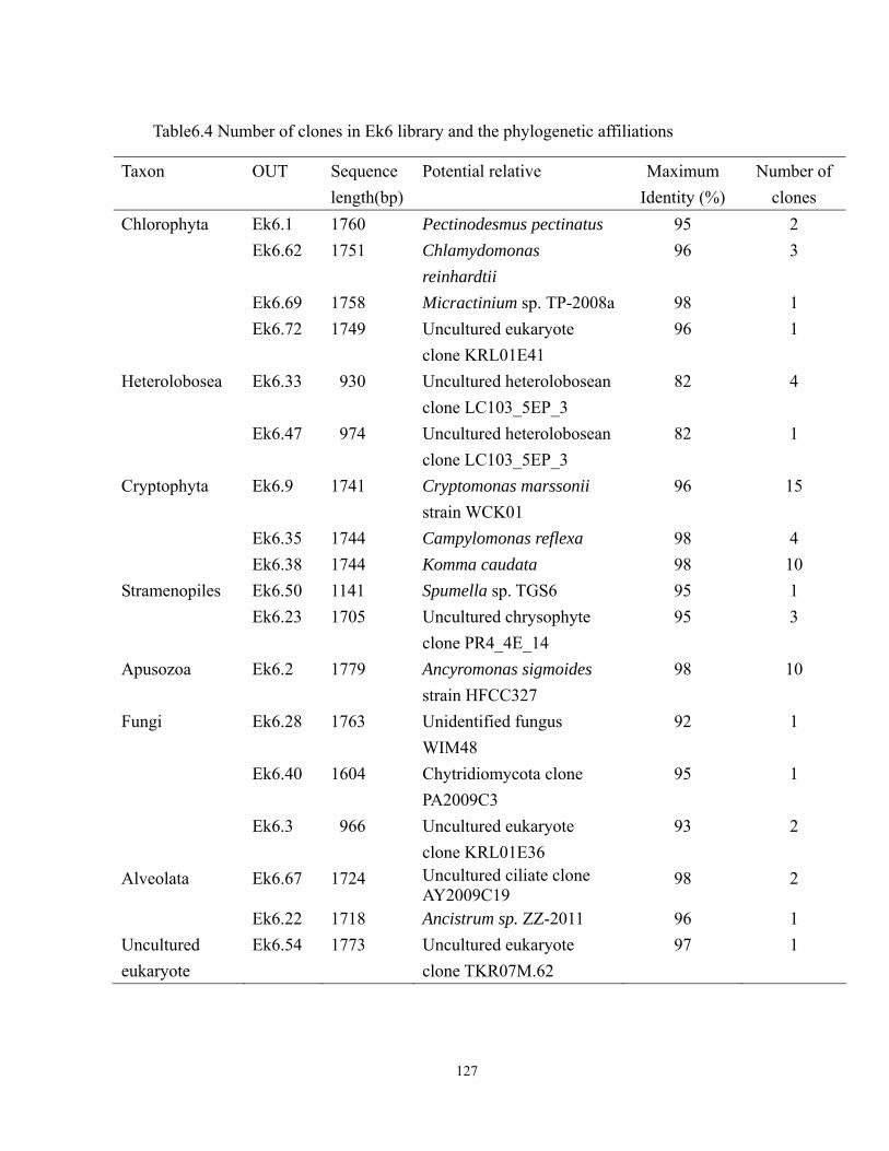
127

Table6.4 Number of clones in Ek6 library and the phylogenetic affiliations

Taxon OUT Sequence length(bp)

Potential relative

Maximum Identity (%)

Number of clones

Chlorophyta Ek6.1 1760 Pectinodesmus pectinatus 95 2 Ek6.62 1751 Chlamydomonas

reinhardtii 96 3

Ek6.69 1758 Micractinium sp. TP-2008a 98 1 Ek6.72 1749 Uncultured eukaryote

clone KRL01E41 96 1


82 4

Ek6.47 974 Uncultured heterolobosean clone LC103_5EP_3

82 1

Cryptophyta Ek6.9 1741 Cryptomonas marssonii strain WCK01

96 15

Ek6.35 1744 Campylomonas reflexa 98 4 Ek6.38 1744 Komma caudata 98 10 Stramenopiles Ek6.50 1141 Spumella sp. TGS6 95 1 Ek6.23 1705 Uncultured chrysophyte

clone PR4_4E_14 95 3

Apusozoa Ek6.2 1779 Ancyromonas sigmoides strain HFCC327

98 10

Fungi Ek6.28 1763 Unidentified fungus WIM48

92 1

Ek6.40 1604 Chytridiomycota clone PA2009C3

95 1

Ek6.3 966 Uncultured eukaryote clone KRL01E36

93 2

Alveolata Ek6.67 1724 Uncultured ciliate clone AY2009C19

98 2

Ek6.22 1718 Ancistrum sp. ZZ-2011 96 1 Uncultured eukaryote

Ek6.54 1773 Uncultured eukaryote clone TKR07M.62

97 1

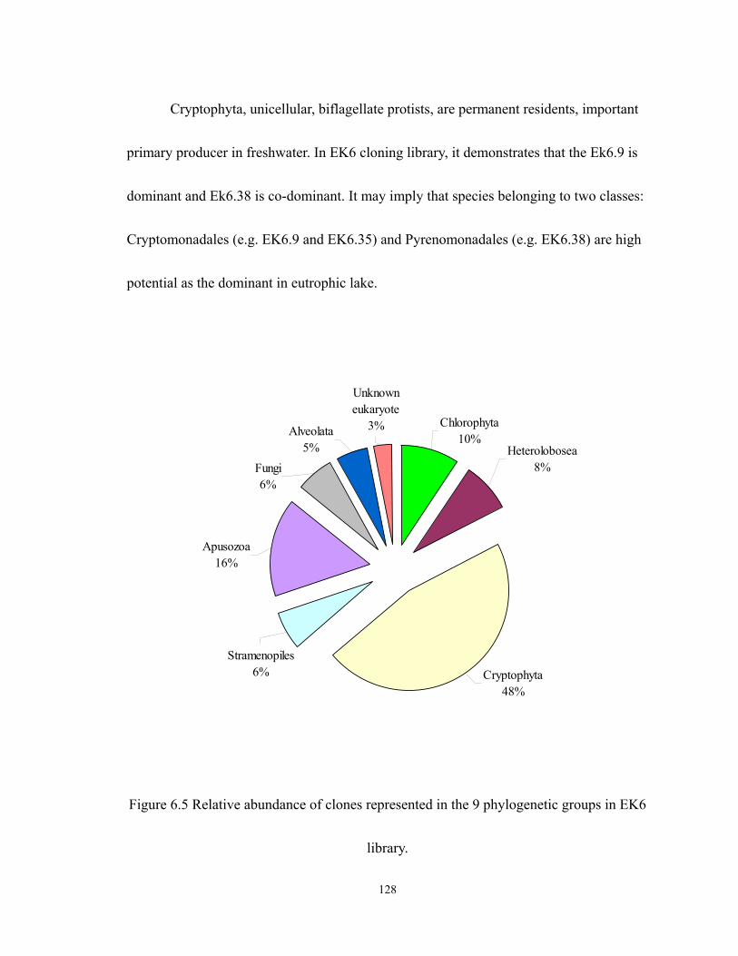
128

Cryptophyta, unicellular, biflagellate protists, are permanent residents, important

primary producer in freshwater. In EK6 cloning library, it demonstrates that the Ek6.9 is

dominant and Ek6.38 is co-dominant. It may imply that species belonging to two classes:

Cryptomonadales (e.g. EK6.9 and EK6.35) and Pyrenomonadales (e.g. EK6.38) are high

potential as the dominant in eutrophic lake.

Unknowneukaryote

3%

Fungi6%

Cryptophyta48%

Heterolobosea8%

Stramenopiles6%

Apusozoa16%

Alveolata5%

Chlorophyta10%

Figure 6.5 Relative abundance of clones represented in the 9 phylogenetic groups in EK6

library.

129

It is very common to describe the population dynamics of cryptophyta in lakes,

but the relationship between cryptophyta and trophic status in lakes is poorly known.

Based on three cloning libraries (EK4, EK5 and EK6), it clearly exhibits that the

populations of the cryptophyta are positively correlated with trophic levels.

The second most abundant group was Apusozoa which obtained 16% of the Ek6

cloning library. In Apusozoa group, 10 clones belonged to the Ek6.2 based on 98%

similarity related to Ancyromonas sigmoides strain HFCC327 identified by Scheckenbach

et al.(Scheckenbach, Wylezich, et al. 2006). The heterotrophic flagellate A. sigmoides

feed on another flagellate as well as bacteria. A. sigmoides has been found in eutrophic

and mesotrophic freshwaters (Kosolapova and Kosolapov 2011; Kosolapova and

Kosolapov 2009; Scheckenbach, et al. 2006).

In Chlorophyta group, four OTUs (Ek6.1, Ek6.62, Ek6.69 and Ek6.72) were

detected. These OTUs obtained more then 95% similarly related to following sequences:

Pectinodesmus pectinatus, Chlamydomonas reinhardtii, Micractinium sp. TP-2008a and

uncultured eukaryote clone KRL01E41, respectively. The potential species are never

detected in other two cloning libraries (EK4 and EK5), except uncultured eukaryote clone

KRL01E41 found in EK5. According to BLAST, three potential species sequences

(Pectinodesmus pectinatus, Scenedesmus regularis and Scenedesmus pectinatus) are

130

closely related to Ek6.1 based on 95% similarity. S. regularis and S. pectinatus are

belonged to the Scenedesmus plankton, which is commonly observed in eutrophic lakes

and ponds (An, Friedl, et al. 1999).

The OUT (EK6.62) is closely related to the sequence of Chlamydomonas

reinhardtii based on 96% similarity. C. reinhardtii, a heterotrophic green alga with two

flagella, is widespread in freshwaters. It is well known to serve as a model organism in

response to the change of environments (e.g. light, nutrient conditions). A study pointed

out that the regulation effort of C. reinhardtii was observed for the yield of algal toxic

while cyanobacterial blooming (Kearns and Hunter 2000). EK6.69 obtained 98%

similarity to the sequence of Micractinium sp. TP-2008a identified by Luo et al. (Luo,

Pröschold, et al. 2010). Micractinium sp. serves as waste-water-grown algal and

commonly occur in waste water treatment systems (Park, Craggs, et al. 2011). Ek6.72 is

related to the sequence of eukaryote clone KRL01E41 sampled from eutrophic Lake

Koronia (Greece) and environment sample KRL01E41 is highly correlated with Carteria

radiosa (D86500) based on the phylogenetic analysis by Oikonomou et al. (Oikonomou,

Katsiapi, et al. 2012).

Ek6.33 and Ek6.47 are affiliated with Heterolobosea phylum and identified only

82% to known sequence (uncultured heterolobosean clone LC103_5EP_3). The sequence

131

of LC103_5EP_3 is detected by López-García et al. (López-García, et al. 2007). It

occurred in extreme environments (e.g. rich carbonate and thermal seawater) according to

López-Garcíass’ work and is also found in EK5 and EK6 cloning libraries in this study.

In Stramenopiles group, two OTUs (Ek6.50 and Ek6.23) were detected and

related to the sequences of Spumella sp. TGS6 and uncultured chrysophyte clone

PR4_4E_14 with 95% similarity. A field study showed that Spumella is abundant in

eutrophic lake (Zhao, Yu, et al. 2003). Rothhaupt’s experiments showed that the

heterotrophic nanoflagellate (HNF) Spumella sp. plays a significant function in the group

role in the transfer of nutrient from bacteria to phytoplankton (e.g. Cryptomonas)

(Rothhaupt 1992). The sequence of PR4_4E_14 is identified by Lara et al.(2011) and

sampled from pristine peat bog under a extreme condition (e.g. low pH value, high

concentration of humic acids, and lack center nutrient) (Lara, et al. 2011). Based on the

Lara’s phylogenetic analysis, although the sequence of the PR4_4E_14 is close related to

Spumella-like, it is assigned to the unidentified eukaryotic lineage, demonstrating that it

is possible to belong the novel clade.

Four clones, comprising three OTUs (EK6.28, EK6.40 and EK6.3), are assigned

to Fungi group which occupied 5% clone abundance in the EK6 cloning library. The

EK6.28 is related to the sequence of fungal WIM48 (novel clade classified) identified by

132

Moon-van der Staay et al. (Moon-van der Staay, Tzeneva, et al. 2006) based on 92%

similarity. In addition, two sequences: KRL01E5 (Oikonomou, et al. 2012) and fungus

clone ESS270706.065 (Masquelier, Hoffman, et al. submitted) found in eutrophic and

mesotrophic lakes, are related to EK6.28. The Ek6.40 related to the sequence of

PA2009C3 identified by Monchy S. et al. (Monchy, et al. 2011). The Ek6.3 linked to

eukaryote clone KRL01E36 (Oikonomou, et al. 2012). According to this study, EK6.3 is

present in three trophic levels (EK4, EK5and EK6 libraries).

In Alveolata group, two OTUs (Ek6.67 and Ek6.22 ) are detected and closely

related to uncultured ciliate clone AY2009C19 (Monchy, et al. 2011) and Ancistrum sp.

ZZ-2011. Ek6.54 is closely related to the sequence of unidentified eukaryote clone

TKR07M.62 originally found in the oligotrophic Lake Tanganyika (Tarbe, et al. 2011).

6.3 Discussion

It is very common in describing the population dynamics of cryptophyta in lakes,

but the relationship between cryptophyta and trophic status in lake is poorly known.

Based on three cloning libraries (EK4, EK5 and EK6), it clearly exhibits that the

populations of the cryptophyta are positively correlated with trophic levels. Compared

with real lakes, the EK4, EK5 and EK6, and PK6 are very similar prokaryotic and

eukaryotic community structure.

133

The species abundance distribution plays a significant role in revealing the

additional dimension of the lake biodiversity. In given assemblage, the distribution

patterns may represent the following desirable aspects: the extent of evenness, which

implies the degree of dominance of certain members, the reason of population fluctuation,

which deduce that physical environment consist of either opportunity species (occasional

species) or equilibrium species (permanent members) and the outcome of population size

stemmed from the mechanisms of competition and predation. The literatures are rich in

respect of the application and mathematic modeling of the species abundance distribution

in the classical ecological diversity study (May 1975; Pielou 1975; Preston 1948), but

limited in respect of the underlying species abundance distribution for eukaryotic and

prokaryotic taxa in lakes. Recently, due to the great progress in the molecular genetic

techniques, the modern ecological tools has offered the contribution to indentify and

number individual and species (Caron, et al. 2004; Caron, et al. 2009). Indeed, more

recently, the OTUs-based species identification and qualification are in widespread use.

For example, the environmental samples collected from different trophic lakes (Lefèvre,

et al. 2007; Lepère, Boucher, et al. 2006; Lepère, Domaizon, et al. 2007; Lepère,

Masquelier, et al. 2010; Luo, Bock, et al. 2011; Mangot, Lepere, et al. 2009), ocean

(Lepère, Vaulot, et al. 2009; Lopez-Garcia, et al. 2001; Moon-van der Staay, et al. 2001)

134

and soil (Bartram, Lynch, et al. 2011; Dunbar, Takala, et al. 1999) have been analyzed by

this approach. The data of OTUs numbered has been regarded as the basic component in

estimating biodiversity index and developing the modeling. For instance, Dunbar

(Dunbar, et al. 2002) has attempted to mathematically describe the relationship between

the number of species and number of individual in soil assemblage by using clones 16S

rDNA gene library.

135

CHAPTER 7. CONCLUSION

The man-made eutrophication problem was expected to be solved through

investigating the relationships between bioproductivity and biodiversity. To date, many

key questions of scientific fundamentals in eutrophication related to the relationships

were far from settled. Using traditional and molecular methods, this research made an

effort to build up reliable laboratory experiments in order to simulate the eutrophic lake

status, to develop a procedure of algal bioproductivity estimates, to unveil the

biodiversity paradox, to obtain more knowledge in trophic levels and their biodiversity, to

analyze the variance in algal bioproductivity and lake biodiversity and to explore the

composition of eukaryotic community under different trophic levels.

The Vollenweider model was adopted as the basic principle to design the lake-like

microcosms called TSCARs. The TSCARs, a CSTR system, provided an environment in

control for algal growth and a basis for estimating algal bioproductivity in the laboratory.

Many behaviors of algal growth and their performance were observed in the system

underlying replicated experiments. Based on community analysis (see Chapter 6),

artificial lake water, BBMM media, is able to provide an environment for prokaryotic and

eukaryotic community structure when compared with real lakes. The three algal growth

136

patterns: pattern I, pattern II, and pattern III were observed and proposed which related to

lake trophic levels (see Chapter3). The phosphorus has a small increase while biomass

(Chl a) approaches its peak when observed by time-varying analysis in higher trophic

levels' bioreactors. It may have resulted from the regeneration of phosphorus. This

suggested that huge populations may be digested and then provide for phosphorus. It

could be evidence to describe how the prokaryotic biodiversity presents huge losses

before reaching a peak of biomass.

A series of equations were developed for the estimates of algal bioproductivity

which were described in Chapter 3. These equations are easy to apply to laboratory and

field investigation.

Based the treatments of experimental design, the algal bioproductivity were

calculated for three trophic levels under TSCARs. The average algal bioproductivity ( rP )

of oligo, meso, and eutrophic levels were 0.37, 0.69, and 2.40 (mg as Chl a /m2 /day);

areal algal product ( TP ) of oligotrophic, mesotrophic, and eutrophic levels were 6.7, 12.5,

and 43.3 (mg as Chl a /m2). The average algal bioproductivity ( rP ) can be converted to

annual carbon bioproductivity by using the ratio of carbon/Chl a between 10 to 182.

Average algal bioproductivity are approximately in agreement with the value of

literature.

137

The lake biodiversity of three trophic levels was investigated. The Shannon index

indicated that the eukaryotic biodiversity of mestrophic level was higher than that of

oligo and eutrotrophic levels. The prokaryotic biodiversity of mestrophic level was lower

than that of oligo and eutrotrophic levels. In comparison, two distinct trophic levels were

identified in Lake Wilson based on TP concentration. Based on investigation, it indicated

that phosphorus regulates the algal growth in two locations (DSTP and WSFP sites) of

Lake Wilson. The eukaryotic biodiversity of DSTP site (higher trophic level) is H’=1.725

while the eukaryotic biodiversity of WSFP site (lower trophic level) is H’=2.571. On the

other hand, the prokaryotic biodiversity of DSTP site is H’=2.861 while the prokaryotic

biodiversity of WSFP site is H’=2.685.

In this dissertation, the phase-oriented concept of the algal growth was proposed

to interpret the varying relationships between lake biodiversity and algal bioproductivity.

The evidence indicated that lake biodiversity can be displayed with variation in algal

bioproductivity. Based on the analysis, there is a general trend that when data were

plotted by eukaryotic biodiversity (H’) against algal bioproductivity (Pr), the relationship

was hump-shaped under phase II and phase III, whereas when data were plotted by

prokaryotic biodiversity (H’) against algal bioproductivity (Pr), the relationship was

U-shaped. During phase I, the eukaryotic biodiversity positively correlated with algal

138

bioproductivity, whereas the prokaryotic biodiversity negatively correlated with algal

bioproductivity. Moreover, several critical timing points of algal growth history in terms

of time-varying Pr(t) revealed a shift in lake biodiversity were proposed. It is a finding

described as the lake biodiversity was deeply affected by the history of algal growth.

By conducting molecular cloning, four libraries (EK4, EK5, EK6, and PK6) were

produced. The community structures sampled from the TSCARs (lake-mimicked

microcosms) were very similar to that of nature lakes. It may provide a direction on an

aspect of methodology for investigating lake eutrophication. In the PK6 library, ten

phylotypes were found and defined as three potential groups: Proteobacteria,

Cyanobacteria, and unidentified environmental samples. In the EK4 library, seventeen

phylotypes were found and defined as ten phylogenetic groups: Chlorophyta,

Heterolobosea, Cryptophyta, Stramenopiles, Cercozoa, Fungi, Rotifera, Amoebozoa,

Alveolata and unidentified eukaryote. The composition of eukaryotic assemblage in a

mesotrophic bioreactor (EK5 library) was investigated showing nine different

phylogenetic groups: Chlorophyta, Heterolobosea, Cryptophyta, Stramenopiles, Cercozoa,

Fungi, Metazoans, Alveolata, and LKM11. In the EK6 cloning library, the eight

phylogenetic groups: Chlorophyta, Heterolobosea, Cryptophyta, Stramenopiles,

Apusozoa, Fungi, Alveolata, and uncultured eukaryote, were detected, which were

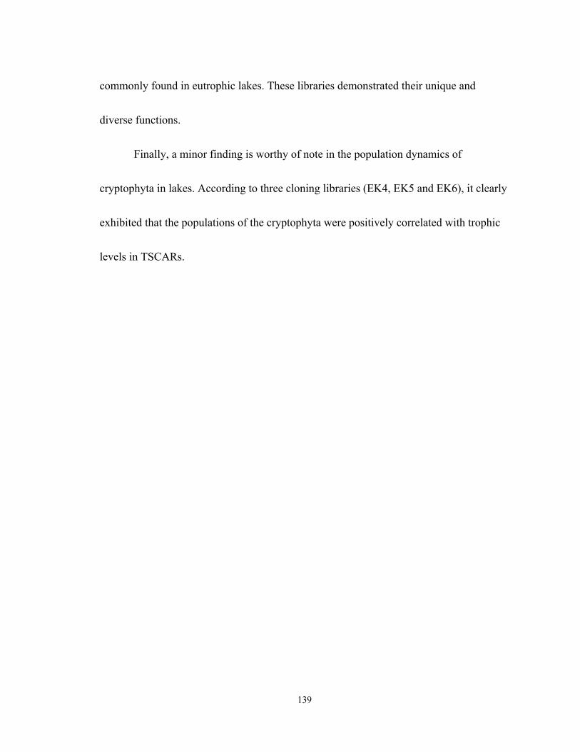
139

commonly found in eutrophic lakes. These libraries demonstrated their unique and

diverse functions.

Finally, a minor finding is worthy of note in the population dynamics of

cryptophyta in lakes. According to three cloning libraries (EK4, EK5 and EK6), it clearly

exhibited that the populations of the cryptophyta were positively correlated with trophic

levels in TSCARs.

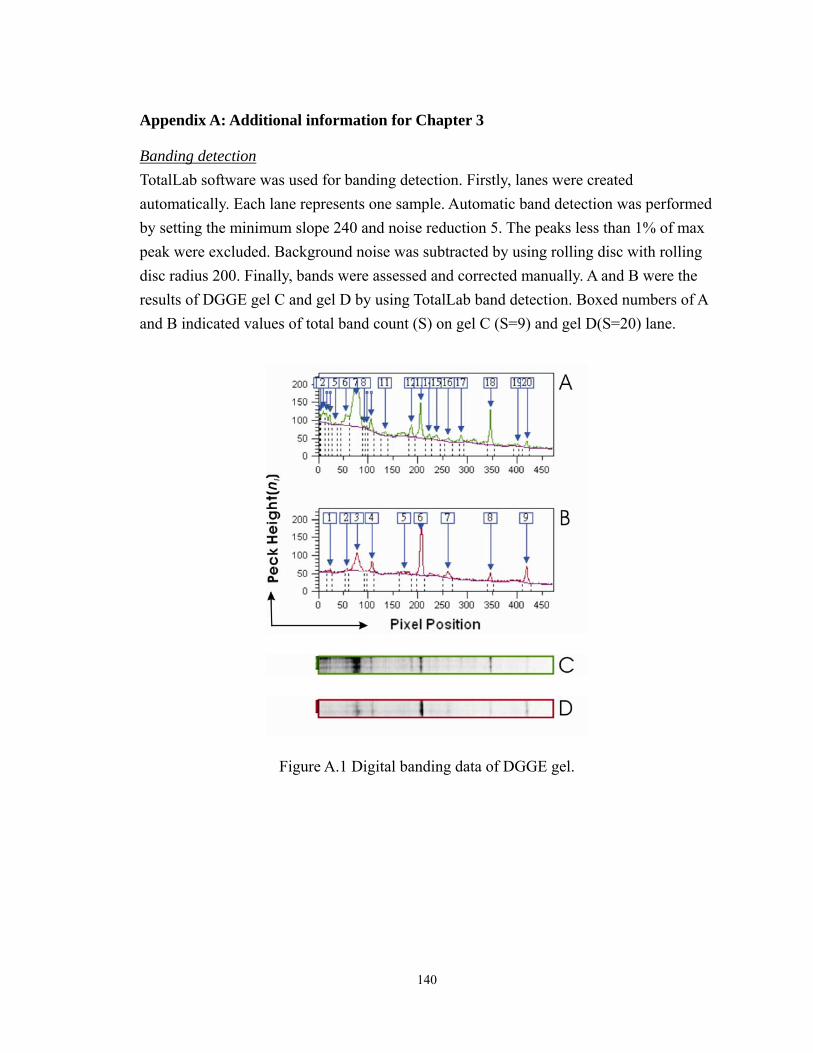
140

Appendix A: Additional information for Chapter 3

Banding detection TotalLab software was used for banding detection. Firstly, lanes were created automatically. Each lane represents one sample. Automatic band detection was performed by setting the minimum slope 240 and noise reduction 5. The peaks less than 1% of max peak were excluded. Background noise was subtracted by using rolling disc with rolling disc radius 200. Finally, bands were assessed and corrected manually. A and B were the results of DGGE gel C and gel D by using TotalLab band detection. Boxed numbers of A and B indicated values of total band count (S) on gel C (S=9) and gel D(S=20) lane.

Figure A.1 Digital banding data of DGGE gel.

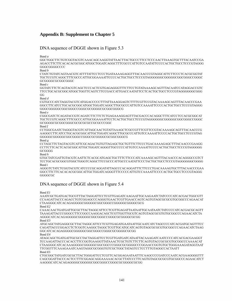
141

Appendix B: Supplement to Chapter 5

DNA sequence of DGGE shown in Figure 5.3

Band a GGCTGGCTTCTGTCGGTACGTCAAACAGCAAGGTATTAACTTACTGCCCTTCCTCCCAACTTAAAGTGCTTTACAATCCGAAGACCTTCTTCACACACGCGGCATGGCTGGATCAGGCTTTCGCCCATTGTCCAATATTCCCCACTGCTGCCTCCCGTAGGGGGGCGGGGCCCC Band b CTATCTGTATCAGTAACGTCATTTTATTCCTCCCTGATAAAAGAGGTTTACAACCCGTAGGCATTCTTCCCTCACGCGGTATTGCTCCGTCAGGCTTTCGCCCATTGCGGAAAATTCCCCACTGCTGCCTCCCGTAGGGGGGCGGGGGCGGCGGGCCGGGCGCGGGGCGCGGCGGGC Band c GGTATCTTCTCAGTACGTCAGCTCCCACTCGTGAGAGGGTTTCTTCCTGTATAAAAGCAGTTTACAATCCATAGGACCGTCTTCCTGCACGCGGCATGGCTGGTTCAGTCTTCCGACCATTGACCAATATTCCTCACTGCTGCCTCCCGTAGGGGGGCGGGGG Band d CGTGCCCATCTAGGTACGTCATGGACCCCCTTTATTAAAGGAGTCTTTTCGTTCCGTACAAAAGCAGTTTACAACCCGAAGGCCTTCATCCTGCACGCGGCATGGCTGGATCAGGCTTGCGCCCATTGTCCAAAATTCCCCACTGCTGCCTCCCGTAGGGGGGCGGGGGCGGCGGGCCGGGCGCGGGGCGCGGCGGGCG Band e CGGCGATCTCAGATACCGTCAGATCTTCTTCTCTGAGAAAGGAGTTTACGACCCACAGGCTTTCATCCTCCACGCGGCATTGCTCCGTCAGGCTTTCGCCCATTGCGGAAAATTCCTCACTGCTGCCTCCCGTAGGGGGGCGGGGGCGGCGGGCCGGGCGCGGGGCGCGGCGGGCGCGCGCGCCGCGCCCGGC Band f CCTGGCGAATCTAGGGTACGTCATTAGCAACTGTATTAAAGCTCGCCGTTTCGTTCCGTACAAAAGCAGTTTACAACCCGAAGGCCTTCATCCTGCACGCGGCATTGCTGGATCAGGCTTGCGCCCATTGTCCAAAATTCCCCACTGCTGCCTCCCGTAGGGGGGCGGGGGCGGCGGGCCGGGCGCGGGGCGCGGCGGGCG Band g CCTAGCTTCTAGTACGTCATTCGCAGACTGTGTTAGAGCTGCTGTTTCTTCCCTGACAAAAGAGCTTTACAACCCGAAGGCCTTCTTCACTCACGCGGCATTGCTGGATCAGGGTTGCCCCCATTGTCCAAAATTCCCCACTGCTGCCTCCCGTAGGGGGGCGGGG Band h GTGCTATCGATTGTACGTCAATTCTCACGCATGAGCTGCTTTCTTCCCATCAAAAGCAGTTTACAACCCACAGGGCCGTCTTCCTGCACGCGGCGTGGCTGGGTCAGGCTTCCGCCCATTGCCCAATATTCCCTACTGCTGCCTCCCGTAGGGGGGCGGGG Band i AGGGTCTATCTCGGTACGTCATCCCCGCAGGATATTAGCCCACAGGATTTCTTCCCTGACAAAAGTGCTTTACAACCCGAAGGCCTTCTTCACACACGCGGCATTGCTGGATCAGGGTTTCCCCCATTGTCCAAAATTCCCCACTGCTGCCTCCCGTAGGGGGGGCGC

DNA sequence of DGGE shown in Figure 5.4

Band E1 AAATCGCTGATGACTGCGTTTACTAGGATTCCTCGTTGAGATCAAGAATTGCAAGAATCTATCCCCATCACGACTGGCGTTCCAAGATTACCCAGACCTGTCGGAGCCCAGGGTGAACTCGTTGAACCAGTCAGTGTAGCGCGCGTGCGGCCCAGAACATCTAAGGGCATCACAGAGGGGCGGGGGCGGCGGGCCGGGGGCGGGGCGCG Band E2 CAAACAACTGATGATTGCGCTTACTAGGCATTCCTCGTTGAGATTAATAATTGCAATAATCTATCCCCATCACGACGCAGTTTAAAGATTACCCGGGCCTTCCGGCCAAGGACAGCTCGTTGGTTGCGTCAGTGTAGCGCGTGTGCGGCCCAGAACATCTAAGGGCATCACAGAGGGGCGGGGGCGGCGGGCCGGGCGCGGGGCGCGG Band E3 ATGCAGCTATGAGGCGCTTACTAGGCATTCCTCGTTGAGATGAATAATTGCAATCATCTAGCCCCATCACGATGCAGTTTCCCAGATTACCCGGACCTCTCGGTCAAGGCTAGGCTCGTTGCATGCATCAGTGTAGCGCGCGTGCGGCCCAGAACATCTAAGGGCATCACAGAGGGGCGGGGGCGGCGGGCCGGGCGCGGGGCGCGG Band E4 ATAGCAGCTGATGATTGCGCCTACTAGGATTCCTCGTTGATGATCATAATTACAAAGATCAATCCCCATCACGACGAAGGTTCCAAGATTACCCACACCTTCCGGTGAAGGTTATAAACTCGCTGTCTTCTTCAGTGTACCGCGCGTGCGGCCCAAAACATCTAAGGGCATCACAAAGGGGCGGGGGCGGCGGCCCGGGCGCGGGGCCCGGAACCGGTGTGCTGGGAAAGATAGGTAATTTCGGTTTCAAAGAAATCAAGTAGGCGCGGGTGTCGCTGGCTATAGTCCTCCTTTGTAGGCCACTAATT Band E5 CTGCGGCTATGATCGCGCTTACTGGGATTCCTCGTTCACGGAGAATAATTTCAAGCCCCGATCCCAATCACGAAGGGGTTTCAGCGGATTACCCACTCCTTTCGGAGCAGGAAAAACACGCTTATCCCTTCAGTGTAGCGCGCGTGCGGCCCAGAACATCTAAGGGCATCACAGAGGGGCGGGGGCGGCGGGCCGGGCGCGGGGCGCGG

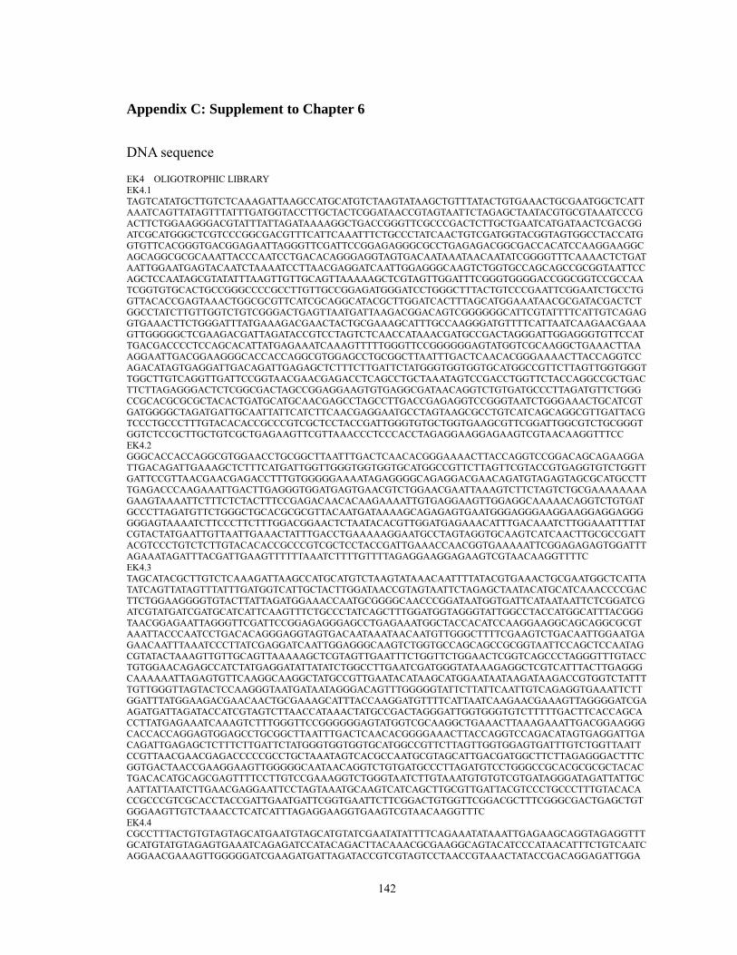
142

Appendix C: Supplement to Chapter 6

DNA sequence

EK4 OLIGOTROPHIC LIBRARY EK4.1 TAGTCATATGCTTGTCTCAAAGATTAAGCCATGCATGTCTAAGTATAAGCTGTTTATACTGTGAAACTGCGAATGGCTCATTAAATCAGTTATAGTTTATTTGATGGTACCTTGCTACTCGGATAACCGTAGTAATTCTAGAGCTAATACGTGCGTAAATCCCGACTTCTGGAAGGGACGTATTTATTAGATAAAAGGCTGACCGGGTTCGCCCGACTCTTGCTGAATCATGATAACTCGACGGATCGCATGGGCTCGTCCCGGCGACGTTTCATTCAAATTTCTGCCCTATCAACTGTCGATGGTACGGTAGTGGCCTACCATGGTGTTCACGGGTGACGGAGAATTAGGGTTCGATTCCGGAGAGGGCGCCTGAGAGACGGCGACCACATCCAAGGAAGGCAGCAGGCGCGCAAATTACCCAATCCTGACACAGGGAGGTAGTGACAATAAATAACAATATCGGGGTTTCAAAACTCTGATAATTGGAATGAGTACAATCTAAAATCCTTAACGAGGATCAATTGGAGGGCAAGTCTGGTGCCAGCAGCCGCGGTAATTCCAGCTCCAATAGCGTATATTTAAGTTGTTGCAGTTAAAAAGCTCGTAGTTGGATTTCGGGTGGGGACCGGCGGTCCGCCAATCGGTGTGCACTGCCGGGCCCCGCCTTGTTGCCGGAGATGGGATCCTGGGCTTTACTGTCCCGAATTCGGAATCTGCCTGGTTACACCGAGTAAACTGGCGCGTTCATCGCAGGCATACGCTTGGATCACTTTAGCATGGAAATAACGCGATACGACTCTGGCCTATCTTGTTGGTCTGTCGGGACTGAGTTAATGATTAAGACGGACAGTCGGGGGGCATTCGTATTTTCATTGTCAGAGGTGAAACTTCTGGGATTTATGAAAGACGAACTACTGCGAAAGCATTTGCCAAGGGATGTTTTCATTAATCAAGAACGAAAGTTGGGGGCTCGAAGACGATTAGATACCGTCCTAGTCTCAACCATAAACGATGCCGACTAGGGATTGGAGGGTGTTCCATTGACGACCCCTCCAGCACATTATGAGAAATCAAAGTTTTTGGGTTCCGGGGGGAGTATGGTCGCAAGGCTGAAACTTAAAGGAATTGACGGAAGGGCACCACCAGGCGTGGAGCCTGCGGCTTAATTTGACTCAACACGGGAAAACTTACCAGGTCCAGACATAGTGAGGATTGACAGATTGAGAGCTCTTTCTTGATTCTATGGGTGGTGGTGCATGGCCGTTCTTAGTTGGTGGGTTGGCTTGTCAGGTTGATTCCGGTAACGAACGAGACCTCAGCCTGCTAAATAGTCCGACCTGGTTCTACCAGGCCGCTGACTTCTTAGAGGGACTCTCGGCGACTAGCCGGAGGAAGTGTGAGGCGATAACAGGTCTGTGATGCCCTTAGATGTTCTGGGCCGCACGCGCGCTACACTGATGCATGCAACGAGCCTAGCCTTGACCGAGAGGTCCGGGTAATCTGGGAAACTGCATCGTGATGGGGCTAGATGATTGCAATTATTCATCTTCAACGAGGAATGCCTAGTAAGCGCCTGTCATCAGCAGGCGTTGATTACGTCCCTGCCCTTTGTACACACCGCCCGTCGCTCCTACCGATTGGGTGTGCTGGTGAAGCGTTCGGATTGGCGTCTGCGGGTGGTCTCCGCTTGCTGTCGCTGAGAAGTTCGTTAAACCCTCCCACCTAGAGGAAGGAGAAGTCGTAACAAGGTTTCC EK4.2 GGGCACCACCAGGCGTGGAACCTGCGGCTTAATTTGACTCAACACGGGAAAACTTACCAGGTCCGGACAGCAGAAGGATTGACAGATTGAAAGCTCTTTCATGATTGGTTGGGTGGTGGTGCATGGCCGTTCTTAGTTCGTACCGTGAGGTGTCTGGTTGATTCCGTTAACGAACGAGACCTTTGTGGGGGAAAATAGAGGGGCAGAGGACGAACAGATGTAGAGTAGCGCATGCCTTTGAGACCCAAGAAATTGACTTGAGGGTGGATGAGTGAACGTCTGGAACGAATTAAAGTCTTCTAGTCTGCGAAAAAAAAGAAGTAAAATTCTTTCTCTACTTTCCGAGACAACACAAGAAAATTGTGAGGAAGTTGGAGGCAAAAACAGGTCTGTGATGCCCTTAGATGTTCTGGGCTGCACGCGCGTTACAATGATAAAAGCAGAGAGTGAATGGGAGGGAAGGAAGGAGGAGGGGGGAGTAAAATCTTCCCTTCTTTGGACGGAACTCTAATACACGTTGGATGAGAAACATTTGACAAATCTTGGAAATTTTATCGTACTATGAATTGTTAATTGAAACTATTTGACCTGAAAAAGGAATGCCTAGTAGGTGCAAGTCATCAACTTGCGCCGATTACGTCCCTGTCTCTTGTACACACCGCCCGTCGCTCCTACCGATTGAAACCAACGGTGAAAAATTCGGAGAGAGTGGATTTAGAAATAGATTTACGATTGAAGTTTTTTAAATCTTTTGTTTTAGAGGAAGGAGAAGTCGTAACAAGGTTTTC EK4.3 TAGCATACGCTTGTCTCAAAGATTAAGCCATGCATGTCTAAGTATAAACAATTTTATACGTGAAACTGCGAATGGCTCATTATATCAGTTATAGTTTATTTGATGGTCATTGCTACTTGGATAACCGTAGTAATTCTAGAGCTAATACATGCATCAAACCCCGACTTCTGGAAGGGGTGTACTTATTAGATGGAAACCAATGCGGGGCAACCCGGATAATGGTGATTCATAATAATTCTCGGATCGATCGTATGATCGATGCATCATTCAAGTTTCTGCCCTATCAGCTTTGGATGGTAGGGTATTGGCCTACCATGGCATTTACGGGTAACGGAGAATTAGGGTTCGATTCCGGAGAGGGAGCCTGAGAAATGGCTACCACATCCAAGGAAGGCAGCAGGCGCGTAAATTACCCAATCCTGACACAGGGAGGTAGTGACAATAAATAACAATGTTGGGCTTTTCGAAGTCTGACAATTGGAATGAGAACAATTTAAATCCCTTATCGAGGATCAATTGGAGGGCAAGTCTGGTGCCAGCAGCCGCGGTAATTCCAGCTCCAATAGCGTATACTAAAGTTGTTGCAGTTAAAAAGCTCGTAGTTGAATTTCTGGTTCTGGAACTCGGTCAGCCCTAGGGTTTGTACCTGTGGAACAGAGCCATCTATGAGGATATTATATCTGGCCTTGAATCGATGGGTATAAAGAGGCTCGTCATTTACTTGAGGGCAAAAAATTAGAGTGTTCAAGGCAAGGCTATGCCGTTGAATACATAAGCATGGAATAATAAGATAAGACCGTGGTCTATTTTGTTGGGTTAGTACTCCAAGGGTAATGATAATAGGGACAGTTTGGGGGTATTCTTATTCAATTGTCAGAGGTGAAATTCTTGGATTTATGGAAGACGAACAACTGCGAAAGCATTTACCAAGGATGTTTTCATTAATCAAGAACGAAAGTTAGGGGATCGAAGATGATTAGATACCATCGTAGTCTTAACCATAAACTATGCCGACTAGGGATTGGTGGGTGTCTTTTTGACTTCACCAGCACCTTATGAGAAATCAAAGTCTTTGGGTTCCGGGGGGAGTATGGTCGCAAGGCTGAAACTTAAAGAAATTGACGGAAGGGCACCACCAGGAGTGGAGCCTGCGGCTTAATTTGACTCAACACGGGGAAACTTACCAGGTCCAGACATAGTGAGGATTGACAGATTGAGAGCTCTTTCTTGATTCTATGGGTGGTGGTGCATGGCCGTTCTTAGTTGGTGGAGTGATTTGTCTGGTTAATTCCGTTAACGAACGAGACCCCCGCCTGCTAAATAGTCACGCCAATGCGTAGCATTGACGATGGCTTCTTAGAGGGACTTTCGGTGACTAACCGAAGGAAGTTGGGGGCAATAACAGGTCTGTGATGCCCTTAGATGTCCTGGGCCGCACGCGCGCTACACTGACACATGCAGCGAGTTTTCCTTGTCCGAAAGGTCTGGGTAATCTTGTAAATGTGTGTCGTGATAGGGATAGATTATTGCAATTATTAATCTTGAACGAGGAATTCCTAGTAAATGCAAGTCATCAGCTTGCGTTGATTACGTCCCTGCCCTTTGTACACACCGCCCGTCGCACCTACCGATTGAATGATTCGGTGAATTCTTCGGACTGTGGTTCGGACGCTTTCGGGCGACTGAGCTGTGGGAAGTTGTCTAAACCTCATCATTTAGAGGAAGGTGAAGTCGTAACAAGGTTTC EK4.4 CGCCTTTACTGTGTAGTAGCATGAATGTAGCATGTATCGAATATATTTTCAGAAATATAAATTGAGAAGCAGGTAGAGGTTTGCATGTATGTAGAGTGAAATCAGAGATCCATACAGACTTACAAACGCGAAGGCAGTACATCCCATAACATTTCTGTCAATCAGGAACGAAAGTTGGGGGATCGAAGATGATTAGATACCGTCGTAGTCCTAACCGTAAACTATACCGACAGGAGATTGGA

143

AGACGAACCCTTTCTCCAGATCCTTTCAGCATTCAAGGGAAACCGAAAGTTTTTAGGTTCTGGGGGGAGTATGGTCGCAAGGCTGAAACTTAAAAGAATTGACGGAAGAACACAACCAGGAGTGGAGTGTGCGGCTTAATTCGACTCAACACGGGAAAACTCACCAGGACCGGATAAACGAGCAGGATTGACAGGTTGAAGTCCTTTCATGATTTCTTATATGGTGGTGCATGGCCGTTCTTAGTACGTGAATTGATTTGTCTGGTTAATTCCGTTAACGTACGAGACCTTAACATATTAATTAGGCAGTCGTTGGTAGTTTACTATCTAATGTTTCTTCGGAAACCGACTTTAGAGCTCCGGCTCTGGCTTCTTAATGGGGACAATGTTACGTTACAAAATATTAGTACAGGGAAGTTTAAGGCAATAACAGGTCTGGAATGCCCTTAGATGTCCTGGGCAGCACGCGTATTACAATGTTAGTTTTAACGAGAAAAAGTTCTCGGATTTATTCGAGAATACCGAGTTTTTTGGTTTACCAAATCTAAAATGACAAGGGAATCTTTTTAATCACCAACGTGACTGGGATAGATGGTTGTAATATCGTCTTCAACGAGGAATTCCTAGTAAGTGCAAGTCACTAACTTGTACTGATTACGTCCCTGTTCTTTGTACACACCGCCCGTCGCTCCTACCAATGGAATAGAAAGATGAAAGAGAAGGACTGGCTTTACCGCTGGGAAATTAATTAAATCTTTCTGTTTGTAGGAAGGAGAAGTCGTAACAAGGTTTTC EK4.5 TAGTCATATGCTTGTCTCAAAGATTAAGCCATGCATGTCTAAGTATAAACTGCTTTATACTGTGAAACTGCGAATGGCTCATTAAATCAGTTATAGTTTATTTGATGGTACCTTACTACTCGGATAACCGTAGTAATTCTAGAGCTAATACGTGCGGAAATCCCGACTTCTGGAAGGGACGTATTTATTAGATAAAAGGCCGACCGGACTCGTCCGACTCGCGGTGAATCATGATAACTCCACGAATCGCATGGCCTCAGCGCCGGCGATGTTTCATTCAAATTTCTGCCCTATCAACTTTCGACGGTAAGGTATTGGCTTACCGTGGTGGTAACGGGTGACGGAGGATTAGGGTTCGATTCCGGAGAGGGAGCCTGAGAAACGGCTACCACATCCAAGGAAGGCAGCAGGCGCGCAAATTACCCAATCTTGACACAAGGAGGTAGTGACAATAAATAACAATACCGGGGTTTTTCAACTCTGGTAATTGGAATGAGTACAATCTAAACCCCTTAACGAGGATCAATTGGAGGGCAAGTCTGGTGCCAGCAGCCGCGGTAATTCCAGCTCCAATAGCGTATATTTAAGTTGTTGCAGTTAAAAAGCTCGTAGTTGGATTTCGGGCGGGCCCGGCCGGTCCGCCTCAGGGTGTGCACTGACCGGGCCCGTCTTGCTGCCGGGGACGGGCTCCTGGGCTTCACTGTCCGGGACCTTCGGAGTCGGCGAGGTTACTTTGAGTAAATTAGAGTGTTCAAAGCAGGCCTACGCTCTGAATACATTAGCATGGAAATAACACGGATAGGACTCTGGCCTATCTTGTTGGTCTGTGGGACCGGAGTAATGATTAGGAGGGACAGTCGGGGGCATTCGTATTTCATTGTCAGAGGTGAAATTCTTGGATTTATGGAAGACGACCTACTGCCGAAGCATTTGCCAAGGGATGTTTTCATTAATCAAGAACGAAAGTCGGGGGCTCGAAGACGATAAAATACGGTCGTAGTCTCAACCATACACGATGCTGACTAGGCATTGGCGGGCGTTCATTTGATGACCCGGCCAGGACCTTATGAGAAATCAAAGTTTTTGGGTTCCGGGGGGAGTATGGTCGCAAGGCTGAAACTTAAAGGAATTGACGGAAGGGCACCACCAGGCGTGGAGCCTGCGGCTTAATTTGACTCAACACGGGAAAACTTACCAGGTCCAGACATAGTGAGGATTGACAGATTGAGAGCTCTTTCTTGATTCTATGGGTGGTGGTGCATGGCCGTTCTTAGTTGGTGGGTTGCCTTGTCAGGTTGATTCCGGTAACGAACGAGACCTCAGCCTGCTAACTAGTCACGATTGGTGCTTCCAGTCGGCCGACTTCTTAGAGGGACTATTGGCGACTAGCCAATGGAAGTGTGAGGCAATAACAGGTCTGTGATGCCCTTAGATGTTCTGGGCCGCACGCGCGCTACACTGATGCGATCAACGAGCCTAGCCTTGGCCGACAGGTCCGGGTAATCTTGCAAACCGCATCGTGATGGGGATAGATGATTGTAATTATTCATCTTCAACGAGGAATGCCTAGTAAGCGCGAGTCATCAGCTCGCGTTGATTACGTCCCTGCCCTTTGTACACACCGCCCGTCGCTCCTACCGATTGGGTGTGCTGGTGAAGCGTTCGGATTGGCGGCAGTGCGCGGTTCGCCGCGTGTTGTAGCCGAGAAGTTCGTTAAACCCTCCCACCTAGAGGAAGGAGAAGTCGTAACAAGGTTTCC EK4.12 AGTCATATGCTTGTCTCAAAGATTAAGCCATGCATGTCTTAGTGTAAATAACTCTTATGAAACTGCGAATGGCTCATTAAATCAGTTATCAAATACGTGATGGTCGCCTACTACATGGATAACCGTAGTAATTCTAGAGCTAATACATGCACAAAGGCCCACGCAAGTGGGTTGTGATTATTAGATTCAAACCGGCCTCGTTCTGGTGATTCATAATAATTGGTCGAACCGCATGCCCTTGTGGTGGCGGTGATTCATCCTTATTTCTGCCCTATCAACTTTCGATGGTAGGATAGAGGCCTACCATGGTTTTAACGGGTGACGGAGAATTAGGGTTCGATTCCGGAGAGGGAGCCTGAGAGACGGCTACCACATCCAAGGAAGGCAGCAGGCGCGCAAATTACCCAATCCCGACTCGGGGAGGTAGTGACAATAAATAACAGTAGAGGGCCAATGGTCTTCTTATTGGAATGAGAACAATTTAAACCCCTTAACGAGGATCAATTAGAGGGCAAGTCTGGTGCCAGCAGCCGCGGTAATTCCAGCTCTAATAGCATATATTAAAGTTGTTGCAGTTAAAAAGCTCGTAGTCGGATTTTGGGCGCGTGTGGGCTGTCGGCCTCTGGTCGGACGGCATGCGCGTGCCTTTCTGCTTGGGAGCCCCATGCGCCGTCCAAGCCGTCGTGCTGGGTCACATGCCGTTTACTATGAAAACATCAGAGCGTCCAAAGCCAGCTATGGCTTGAATAGATTAGCATGGAATAATGGAATACGACCTTGTTGCTACTTCGTCGGTTATGGGACTGGGGTAATGATTAATACGGACAGTCGGGGCCGTTCATATTTCGTTGTCAGAGGTGAAATTCTGGATTTACGAACGATGAACCTTGTGCGAAAGCATTCGGGCAAGGATGTTTTCATTGATCAAGAACGAAAGTTAGGGGATCGAAGACGATCAGATACCGTCGTAAGTCTTAACCATAAACTATGCCAACTAGGGATCAATTGAGTGTCAATTTACGACCTCATTGGCACCTTGTGAGAAATCAAAGTTTATTGGGTTCCGGGGGGAGTATGGTCGCAAGGCTGAAACTTAAAGGAATTGACGGAAGGGCACCACCAGGAGTGGAGCCTGCGGCTTAATTTGACTCAACACGGGGAAACTTACCAGGTCCAGACATAGTCAGGATGGACAGATTGAAAGCTCTTTCTTGATTCTATGGGTGGTGGTGCATGGCCGTTCTTAGTTGGTGGAGTGATTTGTCTGGTTAATTCCGTTAACGAACGAGACCTCGGCCTGCTAACTAGCGATGCCCTTCTTTGAAGGGTAGCCCGCTTCTTAGAGGGACTATTCGTGTTCAACGAATGGAAGTTTGAGGCAATAACAGGTCTGTGATGCCCTTAGATGTTCTGGGCCGCACGCGCGCTACACTGATGGATGCAACGAGCTCTACCCTTGACCGAAAGGCCCGGGTAAACTTGTCAAAATTCATCGTGATGGGGATAGATTATTGCAATTCTTGATCTTCAACGAGGAATTCCTAGTAAGCGCGAGTCATCAGCTCGCGTTGATTACGTCCCTGCCCTTTGTACACACCGCCCGTCGCTCCTACCGATTGAATGGTCCGGCGAAATCTTCAGATTGCTGGCGAGTTCCTCACGGCTCTCGCTGTGAGAAGTTGATTAAACCTTATCATTTAGAGGAAGGAGAAGTCGTAACAAGGTTTC EK4.14 AGTCATATGCTTGTCTCAAAGATTAAGCCATGCATGTCTAAGTATAAACTGCTTTATACTGTGAAACTGCGAATGGCTCATTAAATCAGTTATAGTTTATTTGATGGTACCTTACTACTCGGATAACCGTAGTAATTCTAGAGCTAATACGTGCGGAAATCCCGACTTCTGGAAGGGACGTATTTATTAGATAAAAGGCCGACCGGACTCGTCCGACTCGCGGTGAATCATGATAACTCCACGAATCGCATGGCCTCAGCGCCGGCGATGTTTCATTCAAATTTCTGCCCTATCAACTTTCGACGGTAAGGTATTGGCTTACCGTGGTGGTAACGGGTGACGGAGGATTAGGGTTCGATTCCGGAGAGGGAGCCTGAGAAACGGCTACCACATCCAAGGAAGGCAGCAGGCGCGCAAATTACCCAATCTTGACACAAGGAGGTAGTGACAATAAATAACAATACCGGGGTTTTTCAACTCTGGTAATTGGAATGAGTACAATCTAAACCCCTTAACGAGGATCAATTGGAGGGCAAGTCTGGTGCCAGCAGCCGCGGTAATTCCAGCTCCAATAGCGTATATTTAAGTTGTTGCAGTTAAAAAGCTCGTAGTTGGATTTCGGGCGGGCCCGGCCGGTCCGCCTCAGGGTGTGCACTGACCGGGCCCGTCTTGCTGCCGGGGACGGGCTCCTGGGCTTCACTGTCCGGGACTCGGA-GTCGGCGAGGTTACTTTGAGTAAATTAGAGTGTTCAAAGCAGGCCTACGCTCTGAATACATTAAGCATGGAATAACACGATAGGAACTCTGGCCTATCTTGGTTGGTCTGTGGGGACCGGACTAATGATTAAGAGGGACAGTCGGCGGGCATTCGTATTTCATTGTAGAGGTGAAATTCTGGATTTATGAAAGACGCACTACTGGCGACAGCATTTGCTAAGCATGGTTCTGCATAATCATCAACGAAAGGTAGGAGTGCTCGATGACTATTACATACGATCGTAGTCTCAACCATAACCGATGCCCTGACTACGGATTGTCTGTCGG

144

TTGCATCAGTAACTACGCCGCGAGCACTTTATGAGAAATCAAAGTTTTTGGGTTCCGGGGGGAGTATGGTCGCAAGGCTGAAACTTAAAGGAATTGACGGAAGGGCACCACCAGGCGTGGAGCCTGCGGCTTAATTTGACTCAACACGGGAAAACTTACCAGGTCCAGACATAGTGAGGATTGACAGATTGAGAGCTCTTTCTTGATTCTATGGGTGGTGGTGCATGGCCGTTCTTAGTTGGTGGGTTGCCTTGTCAGGTTGATTCCGGTAACGAACGAGACCTCAGCCTGCTAACTAGTCACGATTGGTGCTTCCAGTCGGCCGACTTCTTAGAGGGACTATTGGCGACTAGCCAATGGAAGTGTGAGGCAATAACAGGTCTGTGATGCCCTTAGATGTTCTGGGCCGCACGCGCGCTACACTGATGCGATCAACGAGCCTAGCCTTGGCCGACAGGTCCGGGTAATCTTGCAAACCGCATCGTGATGGGGATAGATGATTGCAATTATTCATCTTCAACGAGGAATGCCTAGTAAGCGCGAGTCATCAGCTCGCGTTGATTACGTCCCTGCCCTTTGTACACACCGCCCGTCGCTCCTACCGATTGGGTGTGCTGGTGAAGCGTTCGGATTGGCGGCAGTGCGCGGTTCGCCGCGTGTTGTAGCCGAGAAGTTCGTTAAACCCTCCCACCTAGAGGAAGGAGAAGTCGTAACAAGGTTT EK4.16 CCTACGGAAACCTTGTTACGACTTCACCTTCCTCTAAATGATGAGGTTTAAATAACTTTCCACAGTCTAGTCGCCCGAGGGCGTCCAAACCACGGTCCGAAAGTTTCACCGAATCATTCAATCGGTAGGTGCGACGGGCGGTGTGTACAAAGGGCAGGGACGTAATCAACGCGAGCTGATGACCCGCATTTACTAGGAATTCCTCGTTCAAGATTAATAATTGCAATAATCTATCCCTATCACGACATACATTTACAAGATTACCCAGACCTTTCGGACAAGGAAGACTCGCTGCGTATGTCAGTGTAGCGCGCGTGCGGCCCAGGACATCTAAGGGCATCACAGACCTGTTATTGCCCCCAACTTCCTTTGGTTAGTCACCAAAAGTCCCTCTAAGAAGCTTACAGCTATGTTAGACATAGCTGAAACTATTTAGCAGGCGGGGGTCTCGTTCGTTAACGGAATTAACCAGACAAATCACTCCACCAACTAAGAACGGCCATGCACCACCACCCATAGAATCAAGAAAGAGCTCTCAATCTGTCAATCCTCACTATGTCTGGACCTGGTAAGTTTCCCCGTGTTGAGTCAAATTAAGCCGCAGGCTCCACTCCTGGTGGTGCCCTTCCGTCAATTTCTTTAAGTTTCAGCCTTGCGACCATACTCCCCCCGGAACCCAAAGACTTTGATTTCTCTCATGGTGCTGAATTAGCGTTCGTTACAAAACGACTACCAATCCCAAGTCGGCATAGTTTATGGTTAGGACTACGATTGGTATCTAATCATCTTCGATCCCTTAACTTTCGTCCTTGATTAATGAAAACATCGTTGGTAAATGCTTTCGCAGTAGTTCGTCCTCCATAAATCCCAAGAATTTCACCTCTGACAATTGAATACGAATACCCCCAACTATCCCTATTAATCATTACCTTGGAGTACAAACCAACAAAATAGACCAAGGTCCTATCTTATTATTTCCATGCTAATGTATTCAACGGCATAAGCCTGCTTTGAACACCCTATTTTGCTCACAGTAAATGACGAGAATCCCATACCCATTAACTTAAATGGACAGATATGTTTTTCTCGAGGATGGCCTCAGGTCCCAGGTACACAACTCGTTTGAGCCGGACCGAGACCCAAGGCCAGAAATTCAACTACGAGCTTTTTAACTGCAACAACTTTAGTATACGCTATTGGAGCTGGAATTACCGCGGCTGCTGGCACCAGACTTGCCCTCCAATTGATCCTCGATAAGGGATTTAAATTGTTCTCATTCCAATTGCCAGACTAAAAATAGCCCGGCATTGTTATTTATTGTCACTACCTCCCTGTGTCAGGATTGGGTAATTTACGCGCCTGCTGCCTTCCTTGGATGTGGTAGCCATTTCTCAGGCTCCCTCTCCGGAATCGAACCCTAATTCTCCGTTACCCGTTAAAGCCATGGTAGGCCAATACCCTACCATCCAAAGCTGATAGGGCAGAAACTTGAATGAAGCATCGATCCGAAGACCGATCCGAAAGTTATTATGAATCACCATTTACCGGGTTGCCCCGCATTGGTTTCCATCTAATAAATACACCCCTTCCAAAAGTCGGGGTTTGATGCATGTATTAGCTCTAGAATTACTACGGTTATCCAAGTAGCAAGGACCTTCAAATAAACTATAACTGATATAATGAGCCATTCGCAGTTTCACAGTATAGATTTGTTTATACTTAGACATGCATGGCTTAATCTTTGAGACAAGCGTATGCTACTGGCAGGAT EK4.17 AGTCATATGCTTGTCTCAAAGATTAAGCCATGCATGTCTTAGTGTAAATAACTCTTATGAAACTGCGAATGGCTCATTAAATCAGTTATCAAATACGTGATGGTCGCCTACTACATGGATAACCGTAGTAATTCTAGAGCTAATACATGCACAAAGGCTCACGCAAGTGGGTTGTGATTATTAGATTCAAACCAGCCTCGTTCTGGTGATTCATAATAATTGGTCGAACCGCATGCCCTCGAGGTGGCGGTGATTCATCCTTATTTCTGCCCTATCAACTTTCGATGGTAGGATAGAGGCCTACCATGGTTTTAACGGGTGACGGAGAATTAGGGTTCGATTCCGGAGAGGGAGCCTGAGAGACGGCTACCACATCCAAGGAAGGCAGCAGGCGCGCAAATTACCCAATCCCGACTCGGGGAGGTAGTGACAATAAATAACAGTAGAGGGCCAACGGTCTTCTTATTGGAATGAGAACAATTTAAACCCCTTAACGAGGATCAATTAGAGGGCAAGTCTGGTGCCAGCAGCCGCGGTAATTCCAGCTCTAATAGCATATATTAAAGTTGTTGCAGTTAAAAAGCTCGTAGTCGGATTTTGGGCGTGTGTGGGCTATCGGCCTCTGGTCGGATGGCGTGCGCGCGCCTTTCTGCTCGGAATCCCCATGGAGGTTCGCGCCTCTGTTGGTGGGTTCACGGGCCGTTTACTTTGAAAAAATTAGAGTGTTCAAAGCAGGCTATCGCTTGAATAGATTAGCATGGAATAATGGAATAGGACCTTGGTGCTATTTCGTTGGTTATGGGACTGAGGTAATGATTAATAGGGACAGTTGGGGCCGTTCATATTTCGTTGTCAGAGGTGAAATTCTTGGGATTTACGAAACGATGAACTTATGCGAAAGCATTCCGGCAGGGATGTTTTTCATTGATCAAGAACGAAAGTTAAGGGGATCGAAGACGATCAGATACCGTCGTAGTCTTAACCATAAACTATGGCAACTAGGGATCATTGAGTGTCAATCTACGACCTCATTGGCACCTTGTGAGACATCAAGGTTTTGGGGTTCCCGGGGGAGTATGGTCGCAAGGCTGAAACTTAAAGGAATTGACGGAAGGGCACCACCAGGAGTGGAGCCTGCGGCTTAATTTGACTCAACACGGGGAAACTTACCAGGTCCAGACATAGTCAGGATGGACAGATTGAAAGCTCTTTCTTGATTCTATGGGTGGTGGTGCATGGCCGTTCTTAGTTGGTGGAGTGATTTGTCTGGTTAATTCCGTTAACGAACGAGACCTCAGCCTGCTAACTAGCGATGCCCTTCTCGAAGGGTAGCACGCTTCTTAGAGGGACTATTCGTGTTCAACGAATGGAAGTTTGAGGCAATAACAGGTCTGTGATGCCCTTAGATGTTCTGGGCCGCACGCGCGCTACACTGATGGATGCAACGAGCTCTACCCTTGACCGAAAGGCCCGGGTAAACTTGTCAAAATCCATCGTGATGGGGATAGATTATTGCAATTCTTGATCTTCAACGAGGAATTCCTAGTAAGCGCGAGTCATCAGCTCGCGTTGATTACGTCCCTGCCCTTTGTACACACCGCCCGTCGCTCCTACCGATTGAATGGTCCGGCGAAATCTTCGGATTACAGGGGTTCCGTGAGGTTCCCATTGTGAGAAGTTGATTAAACCTTATCATTTAGAGGAAGGAGAAGTCGTAACAAGGTTTC EK4.18 AGTCATATGCTTGTCTCAAAGATTAAGCCATGCATGTCTAAGTATAAACAACTTTATACTGTAAAACTGCGAACGGCTCATTACATCGGCAATAATTTATTTGATGATTTCTTACTACATGGATAACTGTAGTAATTCTAGAGCTAATACATGCGCAAAGTCCTGACTCGCGAGGGGAGGGATGTATTTATTAGATACAAAACCAATGCGGGTTCTGCTCGCCATTGTGTTGAATCATAGTAACTTATCGAACGCCATAGCCTTGTGCTGGGCGTAGATCATTCAAATTTCTGCCCTATCAGCTTTCGACGGTAGTGTAGTGGACTACCGTGGCGTTAACGGGTAACGGGGAATTAGGGTTCGATTCCGGAGAGGGAGCCTGAGAAACGGCTACCACATCCAAGGAAGGCAGCAGGCGCGCAAATTACCCAATCCTGACACAGGGAGGTAGTGACAAAAAATAACAATACCTGGCCTCAATAGGTCGGGTAATTGGAATGAGTACAATTTAAATCCCTTAACGAGGATCAATTGGAGGGCAAGTCTGGTGCCAGCAGCCGCGGTAATTCCAGCTCCAAGAGCATATATTAAAGTTGTTGCAGTTAAAAAGCTCGTAGTTGGATTTCTGGTACAACGCACCTGGCCCGCAGCCATTAGGCTTGTGTGCGCCGGCGCGCGTTTGCCATCCTTCTAGAAAACGGGTCTGCCATTAACTTGGTGGGTTCGCGATCTAGGATCATTTACTTTGAAAAAATTAGAGCTGTTTAAAGCAAGCAATTGCTATGAATACATTAGCATGGAAATAATAATCTAGGACTTCGGTTCTATTTTGTTGGTTTCTAAAACTGAAGTAATGATTGATAGGGACAGTTTGGGGGTGCTAGTATTGGCCCGGCCAGAGGTGAAATTCTTGATTCGGTCAAGACTAACTTATGCGAAAGCATTCACCAAGGGATGTCTTCTTTAATCAAGAACGAAAGGTAGGGGATCGGAGACGATCAGAATACGTCGTAGTCTCAACGATAAACTATGCCAACTAGCAATGG

145

AGTTGACGTTGCTTTTTCGACTTCATCCGCACCTTATGAGAAATCAAAGTCTTTGGGTTCCGGGGGGAGTATGGTCGCAAGGCTGAAACTTAAAGGAATTGACGGAAGGGCACCACCAGGAGTGGAGCCTGCGGCTTAATTTGACTCAACACGGGAAAACTTACCAGGTCCGGACATAGTGAGGATTGACAGATTGAAGATCTTTCTTGATTCTATGGGTGGTGGTGCATGGCCGTTCTTAGTTGGTGGAGTGATTTGTCTGGTTAATTCCGTTAACGAACGAGACCTCGACCTGCTAAATAGTTGACTTAGCTCATCGGGCTTGGATTGACTTCTTAGAGGGACTTTTGGTGGTTAGCTAAAGGAAGTTCGAGGCAATAACAGGTCTGTGATGCCCTTAGATGTTCTGGGCCGCACGCGCGCTACACTGATCGGTTCATCGAGCATACAACCTTGACCGATAGGTCTGGGTAATCTTGTGAAAACCTGATCGTGCTGGGGATAGATCATTGTAATTATTGATCTTCAACGAGGAATTCCTAGTAAACGCGAGTCATCAACTCGCATTGATTACGTCCCTGCCCTTTGTACACACCGCCCGTCGCTACTACCGATTGAATGGCTTAGTGAGCTCTCTGGACTGTTGCGTGTTGGGGCAACTCAACACGCAAATGGGAAGGAGATCAAACTTGATCATTTAGAGGAAGTAAAAGTCGTAACAAGGTTTC EK4.21 AGTCATACGCTCGTCTCAAAGATTAAGCCATGCATGTCTAAGTATAAGCGTTTATACAGTGAAACTGCGAATGGCTCATTATATCAGTTATAGTTTACTTGATAGTGCCTTACTACATGGATAACCGTAGTAATTCTAGAGCTAATACATGCGTAAGTCCCGACCGGCAACGGAAGGGATGTATTTATTAGATATAAGCCAACGCGGTCAGCAATGGCCGGTTTTTGGTGAGTCATAATAACTTTTGCGGATCGCAGTGCGGCTTGCCGCGGCGATGAATCATTCAAGTTTCTGCCCTATCAGCTTTCGATGGTAGGGTATTGGCCTACCATGGCATTAACGGGTAACGGAGAATTAGGGTTCGGTTCCGGAGAGGGAGCCTGAGAAATGGCTACCACCTCCACGGAAGGCAGCAGGCGCGTAAATTACCCAATCCTGACACAGGGAGGTAGTGACAAGAAATAACAAGGCGGGGCTTTCATAGTCTTGCTTTTGGAATGGGGTGAAATTAAATCAATTGCCGAGAACCAATTGGAGGGCAAGCCTGGTGCCAGCAGCCGCGGTAATTCCAGCTCCAATAGCGTATATTAAAGTTGTTGCAGTTAAAAAGCTCGTAGTTGGATTTCTGGAGGGAGCGGCCGGTCCGCGTCCTTTGGGCGCGTGTACTAGCTGTGTCTCCCACCTGCCTTGCGGGGACCGTGTCGTGCGGCTCTGCCGTCGCGGCCGGGAACCGCATCATTTACTGCTGAGAAAATTAGAGTGTTCAAAGCAGGTCTGCGCGTCTTTGAATACGTTAGCATGGAATAATAAGATAGGACTCTGTGCCTATTTTGTTGGTTTGCGAGCCAGAGTAATGATTATACGGATAGTTGGGGGGTATTCGTATTTCATTGTCAGAGGTGAAATTCGTCGATTTCTGAAAGACGAACTACTGCGAAAGCATTTACGAAGGGATGTTTTTCATAATCAGGACCGAAAGTCAGGGGATCGAAGAGGATTAGATACGCTCGTAGTCTGGACAGTAGACTATGCCGACTCGGCATTGCCTGAACGTTGAGTTTAACCGACTCTGTCAGCACCGTATGAAAAATCAAAGTCTTTGGGTTCCGGGGGGAGTATGGTCGCAAGGCTGAAACTTAAAGGAATTGACGGAAGGGCACCACCAGGAGTGGAGCCTGCGGCTTAATTTGACTCAACACGGGAAAACTTACCAGGTCCAGACATAGTAAGGATTGACAGATTGAGAGCTCTTTCTTGATTCTATGGGTGGTGGTGCATGGCCGTTCTTAGTTGGTGGAGTGATTTGTCTGGTTAATTCCGTTAACGAACGAGACCTCCGCCTGCTAAATAGTTCCACTATTCAATTTCGAATGGTGCGGAACTTCTTAGAGGGACAATGGGCGTTCAGCCCGTGGAAGTTGGAGGCAATAACAGGTCTGTGATGCCCTTAGATGTTCTGGGCTGCACGCGCGCTACACTGACAGGTGCAACGAGTTTCAAAGCTCCTTGACCGAGAGGTCTGGGTAATCTTTGAACGCCTGTCGTGATGGGGATAGATTATTGAAATTATTAATCTTCAACGAGGAATTCCTAGTAAACGCAAGTCATCAGCTTGCGTTGATTACGTCCCTGCCCTTTGTACACACCGCCCGTCGCACCTACCGATTGAATGGTCCGGTGAAGTTTTCGGACCGAGACGCAGTTGACCTTCCCAGGTTGATTGCTGTCTTGGGAAGTCACCTAAACCTTACCATTTAGAGGAAGGTGAAGTCGTAACAAGGTCTC EK4.34 CCTACGGAAACCTTGTTACGACTTCACCTTCCTCTAAATGATGAGGTTTAAATAACTTCCCAGCAACCAGCTGCCCGAGGGCCTCTAGTCATCGGTCCGAAAGTTTCACCGAATCATTCAATCGGTAGGTGCGACGGGCGGTGTGTACAAAGGGCAGGGACGTAATCAACGCGAGCTGATGACCCGCATTTACTAGGAATTCCTCGTTCAAGATTAATAATTGCAATAATCTATCCCTATCACGACATACATTTACAAGATTACCCAGACCTTTCGGTCAAGGATAGAGAACCCGAAGGTTCAAAACTCGCTGCGTATGTCAGTGTAGCGCGCGTGCGGCCCAGGACATCTAAGGGCATCACAGACCTGTTATTGCCCCCAACTTCCTTCGATTAGTCACCGAAAGTCCCTCTAAGAAGTCTATTCATTGGATGAATACCCATGCAAAGCATGGGCCCGACTAGTTAGCAGGCGGGGGTCTCGTTCGTTAACGGAATTAACCAGACAAATCACTCCACCAACTAAGAACGGCCATGCACCACCACCCATAGAATCAAGAAAGAGCTCTCAATCTGTCAATCCTCACTATGTCTGGACCTGGTAAGTTTCCCCGTGTTGAGTCAAATTAAGCCGCAGGCTCCACTCCTGGTGGTGCCCTTCCGTCAATTTCTTTAAGTTTCAGCCTTGCGACCATACTCCCCCCGGAACCCAAAGACTTTGATTTCTCCTAAGGTGCTGATGAAGTCATTACAAACGGTCCACCAATCCCTAGTCGGCATAGTTTATGGTTAAGACTACCGATGGTATCTAATCATCTTCGATCCCCTAACTTTCGTTCTTGATTAATGAAAAACATCCTTTGGTAAATGCTTTCGCAGTAGTTCGTCTTCGAGAAATCCAAGAATTTCACCTCTGACACTTGAATACGAATACCCCCCAAACTGTCCCTATTAATCATTACTCGGGACTGCAAACCAACAAAATTAGACCAAGGTCCTATCTTATTATTCCATGCTAATGTAATCCACGGCCTAAGCCTGCGTGACAGCTTGTGATTTTGCTCCACAGGTAACAGATGGGCAGACATGGAGACGACCAGTTAAGGCCACCCCCACACTGAGATCCCAAAAAAGGAGACAAGTAGCATTACAAACCTCTCGCGAGGCGAACACAATCACTTTGTACTCCAGAAATCCAACTACGAGCTTTTTAACTGCAACAACTTTAGTATACGCTATTGGAGCTGGAATTACCGCGGCTGCTGGCACCAGACTTGCCCTCCAATTGATCCTCGATAAGGGATTTAAATTGTTCTCATTCCAATTGCCTAGCCTAGATAGGCCAGGCATTGTTATTTATTGTCACTACCTCCCTGTGTCAGGATTGGGTAATTTACGCGCCTGCTGCCTTCCTTGGATGTGGTAGCCATTTCTCAGGCTCCCTCTCCGGAATCGAACCCTAATTCTCCGTTACCCGTTAAAGCCATGGTAGGCCAATACCCTACCATCCAAAGCTGATAGGGCAGAAACTTGAATGATGCATCGATAAATCGATCCGAAAGTTATTATGAATCACCAAATATACTGGGTTGCCCCATATTGGTTTCCATCTAATAAATACACCCTTTCCATTGCTAGTCAGGGCCTTATGCATGTATTAGCTCTAGAATTACTACGGTTATCCAAGTAGCAAGAACCATCAAAGAAACTATAACTGATATAATGAGCCATTCGCAGTTTCACAGTATATAGTCGTTTATACTTAGACATGCATGGCTTAATCTTTGAGACAAGCGTATGCTACTGGCAGGAT EK4.63 AAATAATAGAATAGGACTTGGATTCTATTTTGGTGGTTTCTAGGACCGAGGTAATGATATAGGACAGTGGGGGCAATTAGTATTCATGTCAGAGTGAAACTGCTTGGATTTATGAAAGACTAAACTACTGCGAAAGCATTTGCCAAGGATGTTTTCATTAATCAAGAACGAAAGTTAGGGGATCGAAGACGATTAGATACCGTCGTAGTCTTAACCATAAACTATGCCGACTCGGGATCGGTGGACTTTATTTTATGAATCCATCGGCACCGTATGAGAAATCAAAGTTTTTGGGTTCTGGGGGGAGTATGGTCGCAAGGCTGAAACTTAAAGGAATTGACGGAAGGGCACCACCAGGAGTGGAGCCTGCGGCTTAATTTGACTCAACACGGGGAAACTCACCAGGTCCAGACATAGTAAGGATTGACAGATTGAGAGCTCTTTCTTGATTCTATGGGTGGTGGTGCATGGCCGTTCTTAGTTGGTGGAGTGATTTGTCTGGTTAATTCCGATAACGAACGGGACCTTAACCTGCTAAATAGGCACAGAAAGTCTTCACTTTCTTGTATGACTTCTTAGAGGGACTATTGGCGTCTAGCCAATGGAAGTTTGAGGCAATAACAGGTCTGTGATGCCCTTAGATGTTCTGGGCCGCACGCGCGCTACACTGATGATGTCAGCGAGTTCTTCCTTGGCCGGAAGGTCTGGGTAATCTTGTGAAACTTCATCGTGCTGGGGATAGAGCATTGCAATTATTGCTCTTCAACGAGGAATTCCTAGTAAGCGCGAGTCATCAGCTCGCGTTGATTACGTCCCTGCCCTTTGTTCACACCGCCCGTCGCTACTACCGATTGAATGGCTTAGTGAGGCCTTGGGATCGCAGAT

146

CAGTCTGGCAACAGAGCTGGTCAGTGAGAACTTGGTCAAACTTGGTCATTTAGAGGAAGTAAAAGTCGTAACAAGGTTTCC EK4.68 ACGGAAACCTTGTTACGACTTTTACTTCCTCTAAATGATCAAGTTTGATCATCTTCTCGGCGCCTAGAGGCGACCTTGCGGCCACTTCCGGACCAATCCGAAGATCTCACTAAACCATTCAATCGGTAGTAGCGACGGGCGGTGTGTACAAAGGGCAGGGACGTAATCAACGCGAGCTTATGACTCGCGCTTACTGGGAATTCCTCGTTCACGGAGAATAATTTCAAGCCCCGATCCCAATCACGAAGGGGTTTCAGCGGATTACCCACTCCTTTCGGAGCAGGAAAAACACGTTCATCCCTTCAGTGTAGCGCGCGTGCGGCCCCGAACATCTAAGGGCATCACAGACCTGTTATTGCTCAATTTCGTGTGGCTTACCGCCACTTGTCCCTCTAAGAAGTACGCGCCGACTAAGGATCGGCGTACTATTTAGCAGGCTAGAGTCTCGTTCGTTATCGGAATTAACCAGACAAATCGCTCCACCAACTAAGAACGGCCATGCACCACCACCCACCGAATCAAGAAAGAGCTCTCAATCTGTCAATCCTTACAGTGTCCGGGCCGGGTGAGATTTCCCGTGTTGAGTCAAATTAAGCCGCAGGCTCCACTCCTGGTGGTGCCCTTCCGTCAATTCCTTTAAGTTTCAGCTTTGCAACCATACTTCCCCCGGAACCCAAAAACTTTGGTTTCCCGGAAGCTGCTAGCTGTGTCGTTTGATTAACAGCAGGGCTATATTCCCTAGTTGGCCATTCGTTATGGTTGGAACTAGGACGGTATCTAATCGTTCTTCGAACCTCCAACTTTCGTTCTTGATTAATGAAAACATTCTTGGCCAATGCTTCGGCAGTTGTTCGTCTTGCGGCGATCCAAGAATTTCACCTCTAACACCGCAATACGAATGCCCCCGTCTGTCCCTATTAATCATTACCTCAATGCTCTACAAAACCAACAAAATAGAACCGAGGTCCTATTCTATTATTCCATGCAACATTATTCAGGCGTAAGGCGTGCTTTAAGCACTCTAATTTTTCTCAAAGTAAACGTTACCGGCCTACCGAAAACACCCAATAAAGGACATCAACGGCCAACCGATGAATTAGGACCGGACATGTAGTGACAGCAGTAAAGCGTACCACATGCCAGTACCCGAGATCCAACTACGAGCTTTTTAACTGCAACAACTTTAATATACGCTATTGGAGCTGGAATTACCGCGGCTGCTGGCACCAGACTTGCCCTCCAATAGATCCTCGTTAAGGGTTTTAAACTGTACTCATTTCAATTACCGAGCCTCATAGAGTCCGGTATTGTTATTTTTCGTCACTACCTCCCCGTTCTAGGAGTGGGTAATTTGCGCGCCTGCTGCCTTCCGTAGATGTGGTAGCCGTTTCTCATGCTCCCTCTCCGGAATCGAACCCTGATTCCCCGTTACCCGTTACAACCATGGTAGGCAGGTCGCTTACCATCGAAAGTTGATAGGGCAGACACTTGAAAGATACGTCGCCGGCTCGAGGCCATGCGATCAGCACAAAGTTATCCAGAGTCACCATACAAAGGGATCTTGCGACCCCATTGGTTTTGGTCTAATAAAAGCGCTCTTCCCATACGGTCGGAGCTTTTTGCATGTATTAGCTCTAGAATTACCACAGTTATCCATGTAATATGAACGATCTAAGGAACCATAACTGATTTAATGAGCCATTCGCGGTTTCACCGTGCAAAGGTATGTACTTAGACATGCATGGCTTAATCTTTGAGACAAGCATATGACTACTGGCAGGAT EK4.76 CCTACGGAAACCTTGTTACGACTTTTACTTCCTCTAAATGATCAAGTTTGATCATCTTCTCGGAACCTAGAGGTAACCTTGCGGCCACTTCCGGACCAATCCGAAGATCTCACTAAACCATTCAATCGGTAGTAGCGACGGGCGGTGTGTACAAAGGGCAGGGACGTAATCAACGCAAGCTTATGACTCGCGCTTACTAGGAATTCCTCGTTCACGGAGAATAATTTCAAGCCCCGATCCCAATCACGAAGGGGTTTCAGCGGGTTACCCACTCCTTTCGGAGCAGGAGAAACACGCTTATCCCTTCAGTGTAGCGCGCGTGCGGCCCCGAACATCTAAGGGCATCACAGACCTGTTATTGCTCAATTTCGTGTAGCTAACCGCTACTTGTCCCTCTAAGAAGTACGCGCCGACTAAAGATCGGCGTACTATTTAGCAGGCTAGAGTCTCGTTCGTTATCGGAATTAACCAGACAAATCGCTCCACCAACTAAGAACGGCCATGCACCACCACCCACCGAATCAAGAAAGAGCTCTCAATCTGTCAATCCTTACAGTGTCCGGGCCGGGTGAGATTTCCCGTGTTGAGTCAAATTAAGCCGCAGGCTCCACTCCTGGTGGTGCCCTTCCGTCAATTCCTTTAAGTTTCAGCTTTGCAACCATACTTCCCCCGGAACCCAAAAACTTTGGTTTCCCGGAAGCTGCTAGCCGTGTCGTTTAATTTACATCGGCTCATATTCGCCAGGCGGCATTCGGTTATGATTGGAACTAGGACGGTATCTAATCGTCTTCGAACCTCCAACTTCCGTTCTTGATTAATGAAAAACATCTTGGCAATTGCTTTCGGCAGTTGTTCGTCTTGCGGCGATTCAAGAATTTCAACTCTAACACCGCAATACGAATGCCCCCGTCTGTCCCTATAAATCATTACCTCAATGCTCTACAAAACCCAACAAAATAGAACCCGAGGTCCTATTCTATTATTCCATGCAACATTATTCAGGCGAATTGCCTGCTTTAAGCACTCTAATTTTCTCAAAGTAAACGTACCGGCTACCGTAAACACCCCAGTAAAGGACATCTACGGCCAACCGATTGATTAGGACCAGACATGTAGTAACAGCAGTTAAGCGTACCACATGCTAGCACCCGAGATCCAACTACGAGCTTTTTAACTGCAACAACTTTAATATACGCTATTGGAGCTGGAATTACCGCGGCTGCTGGCACCAGACTTGCCCTCCAATAGATCCTCGTTAAGGGTTTTAAACTGTACTCATTTCAATTACCGAGCCTCTATGAGTCCGGTATTGTTATTTTTCGTCACTACCTCCCCGTTCTAGGAGTGGGTAATTTGCGCGCCTGCTGCCTTCCGTAGATGTGGTAGCCATTTCTCATGCTCCCTCTCCGGAATCGAACCCTGATTCCCCGTTACCCGTTACAACCATGGTAGGCAGGTCGCTTACCATCGAAAGTTGATAGGGCAGACACTTGAAAGATACGTCGCCGGCTCGAGGCCATGCGATCAGCACAAAGTTATCCAGAGTCACCAGACAAAGGGATGTCGCCACCCCATTGGTTTTGGTCTAATAAAAGCGCTCTTCCCATACGGTCGGAGCTTTTTGCATGTATTAGCTCTAGAATTACCACAGTTATCCATGTAATATGAACGATCTAAGGAACCATAACTGATTTAATGAGCCATTCGCGGTTTCACCGTGCAAAGGTATGTACTTAGACATGCATGGCTTAATCTTTGAGACAAGCATATGACTACTGGCAGGAT EK4.77 GGGTAAGTAGATTAGCCATGCATGTCTAAGTTTAGTATTAAACAGCGAAACTGCGAATGGCTCATTAAATCAGTTATAATCTACTCGATCAACACTATCTTTACTCGGATAACTGTAGTAATTCTAGAGCTAATACGTGCACTAAAGGCCTGACTTTCGGGAAGGGCCGCGCTTGTTAGATTCCACACCGACCAGGGTAACCTGAGCTTTGGTGATTCTAGCCAAGATAGCAGATCGCATAGCCTCGTGCTGGCGACAGTTCGATCGAGTTTCTGCCCTATCAACTAGATTGTAGTGTATTGGACTACAATGGTGATAACGGGTGACGGGGAATTAGGGTTCGGTTCCGGAGAGGGAGCCTGAGAAATGGCTACCACTTCCAAGGAAGGCAGCAGGCGCGCAAATTACCCAATGTCAATTCGACGAGGTAGTGACAATAAATAACAATCCCGAGCCTTCTAGGCCTGGGAATTGGAATGAGTACAACGTAAATAACTTAACGAGGAACCATTGGAGGACAAGTCTGGTGCCAGCACCCGCGGTAATTCCAGCTCCAATAGCGTATATTAAAGTTGTTGCAGTTAAAAAGCTCGTAGTTGGATTCGAAGCGTCTTAGTTGGCCGAGAGGATGGTTGGACCTTTACGGCATGTACTAGTACGTTCTACGTTCAGGTCGATGTTGACTTGACCTTATTCGCTGGTCTTACGTCCTGGACCGTTTACCTTGGATTAACTAAGGTGTTCAAAGGCAGCTTTAAAAGGCTGGATTAGTTTAGCATGGGGATAATGGAATACGACTCTAGCCAGTCCGTCGGTGTTTCTGGTCAGGGTAATGATTAATAGAGATAGTCGGGGTCATTCATATTCAATTGTCAGAGGTGAAATTCTTAGATTCTTTGAAGATGAACTGCAGCGAAAGCGTTTGACAAGGGATGCTCTCATTAATCAAGAACGAAAGTTAGGGGATCGAAGACGATCAGATACCGTCGTAGTCTTAACTATAAACGATACGAATCGAGGATTGGATGATGTTAATCGTACGACTTTTTCGGAACTTCAGGAGAAATCTTTGAATCTTGCCGTTCTGGGGGGAGTATGGTCGCAAGGCTGAAACTTAAAGGAATTGACGGAAAGGGCACACCAGGAGTGGAGCCTGCGGCTTAATTTGACTCAACACGGGAAAACTTACTAGGTCAGAACATGGTTATGATTGACAGATTGATAGCTCTTTCTTAATTTCTATGGGTGGTGGTGCATGGCCGTTCTTAGTTGGTGGAGTGATTTGTCTGGTTAATTCCGATAACGAACGAGATCGCATCCTACTAAATAGTGGCCCTAATCGTCTATATGGGTGAAGCAGGTCGGTGCTGTGGCGCTGGGAAACTGGCCGCTATAGTCTTTCCTGGGGATCCTTGATGTATTGGGGTCAAATTACTTCTTAGAGGGACTGTCGGCGATTAGCCGAAGGAAGTGCGGCAATAACAGGTCTGTGATGCCCTTAGATGTCCTAGGCTGCACGCGCGCTAC

147

ACTGTCTGGTACAATGAGTCTACAATGCTGGTCCGATAGGATTGGCGAATCTTGTGAATGCTTGACGTGATGGGGATTGATCATTGAAATTATTGGTCATGAACGAGGAATTCCTTGTAGGTATGCTTCATCAAAGCATGCCGACTACGTCCCTGCCCTTTGTACACACCGCCCGTCGCTCCTACCGATTGAGTGATCAGATGAAATCCGCGGACTCGAGTCGGCTTGCCGATGCGGGGAAGTTGAGTAAATCTTATGCTAGAGAAGAGAGTCAGACTCGC EK4.79 AGTCATATGCTTGTCTTGAAGACTAAGCCATGCATGTCTAAGTATAAATAGTATACAGTGAAACTGCGAATGGCTCATTAAAACAGTTATAGTTTACTTGATAATTGAATTCTACATGGATAACCGTGGTAATTCTAGGGCTAATACATGCGGCAAAACCCAACTTTTCGGAAGGGTTGTATTTATTAGATAACAAACCAATATTCCTTCGGGTCTATTGTGATGATTCATAGTAACTGATCGGAGCGCGACTCGTTGCGCTAAATCATTCAAGTTTCTGCCCTATCAGCTTTCGATGGTAGTGTATTGGACTACCATGGCAGTCACGGGTAACGGGGAATTAGGGTTCGATTCCGGAGAGGGAGCCTGAGAAACGGCTACCACATCTAAGGAAGGCAGCAGGCGCGTAAATTACCCAATCCTAATTCAGGGAGGTAGTGACAAGAAATAACAAACCGGGTTCTTACGAACTTTGGGATTGCAATGAGCACAATTTAAATCTCTTAGCAAGGAACAATTGGAGGGCAAGTCTGGTGCCAGCAGCCGCGGTAATTCCAGCTCCAATAGCGTATATTAAAGTTGTTGCAGTTAAAAAGCTCGTAGTTGAACTTCTGGGCGTCTGTACAGCGGCTCCGGTCGAGGTATAGGCGTTCATCCGTCTGAGAACCATATACGGCCTTTAGTGGTCGGTGTGAGAATTCCAGGCACCTTACTTTGAAAAACTTAGAGTGGTTCCAGGCAGGCAATCGCCTTGAATACACAAGCATGGAATTATTGAATAGGACTATGGTCCATTTTGTAGGTTATTGGGCTATAGTAATGATTAACAGGAACGGCCCGGGGGTGATTTGTATTTAATAGTCAGAGGTGAAAATCTTGGATTTATTAAAGACAAACTAAAGCGAACGCTTTTCACAAGAGCGTTTTCATTAATCAAGAACGAAAGTTAGGGGATCAAAGACGATCAGATACCGTCCTAGTCTTAACCATAAACTATTCCGACTAGGGATTGGTCGGGTCTTTCAAGCCCGATCAGCACCTTATGAGAAATCAAAGTCTTTGGGTTCCGGGGGGAGTATGGTCGCAAGGCTGAAACTTAAAGGAATTGACGGAAGGGCACCACCAGGAGTGGAGCCTGCGGCTTAATTTGACTCAACACGGGGAAACTCACCAGCGCAAAACATGGGTGGGATTGACAGATTGAGAGCTCTTTCTTGATTCTATGGGTGGTGGTGCATGGCCGTTCTTAGTTGGTGGAGTGATTTGTCTGGTTAATTCCGTTAACGAACGAGACCTTAACCTGCTAACTAGTCTCCTTATGAACAATGGGGAGGACTTCTTAGAGGGACTATGTGAACAAACACATGGAAGTTTGAGGCAATAACAGGTCTGTGATGCCCTTAGATGTGCTGGGCCGCACGCGCGCTACAATGATACGTTCAGCAAGTTCTATCCTGGTCCGGAAGGATTCGGGTAATCTTGGCAACGCGTATCGTGCTGGGGATCGATCTTTGCAATTATAGATCTTGAACGAGGAATTCCTAGTAAGTGCAAGTCATCAGCTTGTACTGATTATGTCCCTGCCCTTTGTACACACCGCCCGTCGCTCCTACCGATTTCGAGTGATCCGGTGAACCTTCTGGACCGAATTGGTCTTCATGGTCAAATTGGGAAGTTAAGTAAACCTTATCACTTAGAGGAAGGAGAAGTCGTAACAAGGTTTC EK5 MESOTROPHIC LIBRARY EK5.1 AGTCATATGCTTGTCTCAAAGATTAAGCCATGCATGTCTTAGTGTAAATAACTCTTATGAAACTGCGAATGGCTCATTAAATCAGTTATCAAATACGTGATGGTCGCCTACTACATGGATAACCGTAGTAATTCTAGAGCTAATACATGCACAAAGGCTCACGCAAGTGGGTTGTGATTATTAGATTCAAACCAGCCTCGTTCTGGTGATTCATAATAATTGGTCGAACCGCATGCCCTCGAGGTGGCGGTGATTCATCCTTATTTCTGCCCTATCAACTTTCGATGGTAGGATAGAGGCCTACCATGGTTTTAACGGGTGACGGAGAATTAGGGTTCGATTCCGGAGAGGGAGCCTGAGAGACGGCTACCACATCCAAGGAAGGCAGCAGGCGCGCAAATTACCCAATCCCGACTCGGGGAGGTAGTGACAATAAATAACAGTAGAGGGCCAACGGTCTTCTTATTGGAATGAGAACAATTTAAACCCCTTAACGAGGATCAATTAGAGGGCAAGTCTGGTGCCAGCAGCCGCGGTAATTCCAGCTCTAATAGCATATATTAAAGTTGTTGCAGTTAAAAAGCTCGTAGTCGGATTTTGGGCGTGTGTGGGCTATCGGCCTCTGGTCGGATGGCGTGCGCGCGCCTTTCTGCTCGGAATCCCCATGGAGGTTCGCGCCTCTGTTGGTGGGTTCACGGGCCGTTTACTTTGAAAAAATTAGAGTGTTCAAAGCAGGCTATCGCTTGAATAGATTAGCATGGAATAATGGAATAGGACCTTGGTGCTATTTCGTTGGTTATGGGACTGAGGTAATGATTAATAGGGACAGTTGGGGCCGTTCATATTTCGTTGTCAGAGGTGAAATTCTTGGGATTTACGAAACGATGAACTTATGCGAAAGCATTCCGGCAGGGATGTTTTTCATTGATCAAGAACGAAAGTTAAGGGGATCGAAGACGATCAGATACCGTCGTAGTCTTAACCATAAACTATGGCAACTAGGGATCATTGAGTGTCAATCTACGACCTCATTGGCACCTTGTGAGACATCAAGGTTTTGGGGTTCCCGGGGGAGTATGGTCGCAAGGCTGAAACTTAAAGGAATTGACGGAAGGGCACCACCAGGAGTGGAGCCTGCGGCTTAATTTGACTCAACACGGGGAAACTTACCAGGTCCAGACATAGTCAGGATGGACAGATTGAAAGCTCTTTCTTGATTCTATGGGTGGTGGTGCATGGCCGTTCTTAGTTGGTGGAGTGATTTGTCTGGTTAATTCCGTTAACGAACGAGACCTCAGCCTGCTAACTAGCGATGCCCTTCTCGAAGGGTAGCACGCTTCTTAGAGGGACTATTCGTGTTCAACGAATGGAAGTTTGAGGCAATAACAGGTCTGTGATGCCCTTAGATGTTCTGGGCCGCACGCGCGCTACACTGATGGATGCAACGAGCTCTACCCTTGACCGAAAGGCCCGGGTAAACTTGTCAAAATCCATCGTGATGGGGATAGATTATTGCAATTCTTGATCTTCAACGAGGAATTCCTAGTAAGCGCGAGTCATCAGCTCGCGTTGATTACGTCCCTGCCCTTTGTACACACCGCCCGTCGCTCCTACCGATTGAATGGTCCGGCGAAATCTTCGGATTACAGGGGTTCCGTGAGGTTCCCATTGTGAGAAGTTGATTAAACCTTATCATTTAGAGGAAGGAGAAGTCGTAACAAGGTTTC EK5.3 AGTCATATGCTTGTTTCAAAGATTAAGCCATGCATGTCTAAGTATAAGCTGCTTATACTGTGAAACTGCGAATGGCTCATTAAATCAGTTATAGTTTATTTGATGGTACCTTACTACTCGGATAACCGTAGTAATTCTAGAGCTAATACGTGCGCACATCCCGACTTCTGGAAGGGACGTATTTATTAGATAAAGACCGACCGGCTCTGCCGACCCTCGGTGAATCATGATAACTTCACGAATCGCATGGCCTCGTGCCGGCGATGTTTCATTCAAATTTCTGCCCTATCAACTTTCGATGGTAGGATAGAGGCCTACCATGGTGTTAACGGGTGACGGAGAATTAGGGTTCGATTCCGGAGAGGGAGCCTGAGAAACGGCTACCACATCCAAGGAAGGCAGCAGGCGCGCAAATTACCCAATCCCGACACGGGGAGGTAGTGACAAAAAATAACAATACTTGGCTCATTCGAGTCCGGTAATTGGAATGAGTACAATCTAAACCCCTTAACGAGGATCCATTGGAGGGCAAGTCTGGTGCCAGCAGCCGCGGTAATTCCAGCTCCAATAGCGTATATTTAAGTTGCTGCAGTTAAAAAGCTCGTAGTCGGTTTTCGGGAGGGGTGGCACGGTCCGCCTTGCGCGTGCACTGCGCCGCCCCTCTTTACCGCTGGTGACCAGCTCCTGGGCCTGGCTGTCCGGGACTCGGAGTCAGCACAGTCACCTTGAGGTATTCGGAGCGGTTCCAATGCAAGCAAACGCTGTGCACCACTTAGGCATGGAATAACGATCAATGGGACTCGCGTCCAGTCGTGGGTCTATGGTCAGGCGAGTAACGACCAATGGGGGCAGTCGGGGGCATTTGTATGGCGGTGTCAGAGGGTGAAATTCTTGGATTTCCGCAAGACAAACAGCTGCGAAAGCGTCCGCCAAGGATGCTTTCGTCGATCAAGAACGAAAGTTGGGGGCTCGAAGACGATTAGATACCGTCCTAGTCTCAACCATAAACGATGCCTGACTAGGGATCGGCGAGGGTTCTATCAACGACCTTCGCCGGCACCTCATGAGAAATCAAAGTGTTTGGGTTCCGGGGGGAGTATGGTCGCAAGGCTGAAACTTAAAGGAATTGACGGAAGGGCACCACCAGGCGTGGAGCCTGTGGCTTAATTTGACTCAACACGGGAAACCTTACCAGGTCCAGACATAGTGAGGATTGACAGATTGAGAGCTCTTTCTTGATTCTATGGGTGGTGGTGCATGGCCGTTCTTAGTTGGTGGGTTGCCTTGTCAGGTTGATTCCGGTAACGAACGAGACCTCAGCCGCTAAATAGTCACTTCCGGTTCGCCGGTCGGTAGACTT

148

CTTAGAGGGACTTTCACCGTCTAGGTGAAGGAAGCATGAGGCGATAACAGGTCTGTGATGCCCTTAGATGTTCTGGGCCGCACACGCGCTACACTGACGCAACCAACGAGCTGTCCTTGGCCGGAAGGCCCGGGTAATCTCTAAACTGCGTCGTGATGGGGATAGATTATTGCAATTATTAATCTTCAACGAGGAATGCCTAGTAAGCGCAAGTCATCAGCTTGCGTTGATTACGTCCCTGCCCTTTGTACACACCGCCCGTCGCTCCTACCGATTGGGTGTGCTGGTGAAGCGTTCGGATTGGCGACTTCGACGGGCAACCGCCGTCGTCGCCGAGAAGTTCTCTAAACCCTCCCACCTAGAGGAAGGAGAAGTCGTAACAAGGTTTC EK5.7 AGTCATATGCTTGTCTCAAAGATTAAGCCATGCATGTCTAAGTATAAACTGCTTTATGCGGTGAAACTGCGAATGGCTCATTAAATCAGTTATAGTTTATTTGATGGTACCTGGTACTCGGATAACTGTACCAAAAGTAGAGCTAATACGTGCGTAAATCCCGACTCACGAAGGGACGTATTTATTAGATAAAAGGCCAGCCGGGCTTGCCCGACTTGTGGTGACTCATGATAACTTCACGAATCGCATGGCCTCGCGCCGGCGATGTTTCATTCAAATTTCTGCCCTATCAACTTTCGATGGTAGGATAGAGGCCTACCATGGTGGTAACGGGTGACGGAGGATTAGGGTTCGATTCCGGAGAGGGAGCCTGAGAAATGGCTACCACATCCAAGGAAGGCAGCAGGCGCGCAAATTACCCAATCCCGACACGGGGAGGTAGTGACAATAAATAACAATACTGGGCATTTTTGTCTGGTAATTGGAATGAGTACAATCTAAATCCCTTAACGAGTATCCATTGGAGGGCAAGTCTGGTGCCAGCAGCCGCGGTAATTCCAGCTCCAATAGCGTATATTTAAGTTGTTGCAGTTAAAAAGCTCGTAGTTGGATTTCGGGTTGGTTCCTGCGGTCCGCCTCTGGTGAGTACTGCTGGGACCTACCTTTCTGTCGGGGACGGGCTCCTGGGCTTAACTGTCCGGGACTCAGGGAGTCGACGAGGATACTTTGAGTAAATTAGAGGGTTCACAGCAGGCCTATGCTCTGAATACGTTAGCATGGAATAACACGATAGGACTCTGGCCTATCTGTGTTGGTCTGTGGGACCCGGAGTAATGAATAGAAGGGACAGTCGGGGGCATTCGTATTTCATTGTCAGAGGTGGAAATCTTGGATTTATGGAAAGACGAACTTCTGCGAAAGCATTGCCAAGGGATGTTTTTCATAATCAAGAACGAAAGTTGGGGCTCGAAGACGATTAGATACCGTCGTAGTCTCAACCATAAACGATGCCGACTAGGGATTGGCAGGCGTTTTGTTAACGACCCTGCCAGCACCTTATGAGAAATCAAAGTTTTTGGGTTCCGGGGGGAGTATGGTCGCAAGGCTGAAACTTAAAGGAATTGACGGAAGGGCACCACCAGGCGTGGAGCCTGCGGCTTAATTTGACTCAACACGGGGAAACTTACCAGGTCCAGACACGGGGAGGATTGACAGATTGAGAGCTCTTTCTTGATTCTGTGGGTGGTGGTGCATGGCCGTTCTTAGTTGGTGGGTTGCCTTGTCAGGTTGATTCCGGTAACGAACGAGACCTCAGCCTGCTAAATAGTCACGACTGCTTTTTGCAGTCGGCTGAACTTCTTAGAGGGACTATTGGCGTTTAGCCAATGGAAGTATGAGGCGATAACAGGTCTGTGATGCCCTTAGATGTTCTGGGCCGCACGCGCGCTACACTGATGCAATCAACGAGCCTATCCTTGGCCGAGAGGCCCGGGTAATCTTTGAAACTGCATCGTGATGGGGATAGATCATTGCAATTATTGGTCTTCAACGAGGAATGCCTAGTAAGCGCAAGTCATCAGCTTGCGTTGATTACGTCCCTGCCCTTTGTACACACCGCCCGTCGCTCCTACCGATTGAGTGTGCTGGTGAAACGTTCGGATCGACGTTTTTGGCTGGCAACAGTCGAAATCGTTGAGAAGTTCATTAAACCCTCCCACTTAGAGGAAGGAGAAGTCGTAACAAGGTTTC EK5.16 TAGTCATATGCTTGTCTCAAAGATTAAGCCATGCATGTCTAAGTATAAGCTGTTTATACTGTGAAACTGCGAATGGCTCATTAAATCAGTTATAGTTTATTTGATGGTACCTTGCTACTCGGATAACCGTAGTAATTCTAGAGCTAATACGTGCGTAAATCCCGACTTCTGGAAGGGACGTATTTATTAGATAAAAGGCTGACCGGGTTCGCCCGACTCTTGCTGAATCATGATAACTCGACGGATCGCATGGGCTCGTCCCGGCGACGTTTCATTCAAATTTCTGCCCTATCAACTGTCGATGGTACGGTAGTGGCCTACCATGGTGTTCACGGGTGACGGAGAATTAGGGTTCGATTCCGGAGAGGGCGCCTGAGAGACGGCGACCACATCCAAGGAAGGCAGCAGGCGCGCAAATTACCCAATCCTGACACAGGGAGGTAGTGACAATAAATAACAATATCGGGGTTTCAAAACTCTGATAATTGGAATGAGTACAATCTAAAATCCTTAACGAGGATCAATTGGAGGGCAAGTCTGGTGCCAGCAGCCGCGGTAATTCCAGCTCCAATAGCGTATATTTAAGTTGTTGCAGTTAAAAAGCTCGTAGTTGGATTTCGGGTGGGGACCGGCGGTCCGCCAATCGGTGTGCACTGCCGGGCCCCGCCTTGTTGCCGGAGATGGGATCCTGGGCTTTACTGTCCCGAATTCGGAATCTGCCTGGTTACACCGAGTAAACTGGCGCGTTCATCGCAGGCATACGCTTGGATCACTTTAGCATGGAAATAACGCGATACGACTCTGGCCTATCTTGTTGGTCTGTCGGGACTGAGTTAATGATTAAGACGGACAGTCGGGGGGCATTCGTATTTTCATTGTCAGAGGTGAAACTTCTGGGATTTATGAAAGACGAACTACTGCGAAAGCATTTGCCAAGGGATGTTTTCATTAATCAAGAACGAAAGTTGGGGGCTCGAAGACGATTAGATACCGTCCTAGTCTCAACCATAAACGATGCCGACTAGGGATTGGAGGGTGTTCCATTGACGACCCCTCCAGCACATTATGAGAAATCAAAGTTTTTGGGTTCCGGGGGGAGTATGGTCGCAAGGCTGAAACTTAAAGGAATTGACGGAAGGGCACCACCAGGCGTGGAGCCTGCGGCTTAATTTGACTCAACACGGGAAAACTTACCAGGTCCAGACATAGTGAGGATTGACAGATTGAGAGCTCTTTCTTGATTCTATGGGTGGTGGTGCATGGCCGTTCTTAGTTGGTGGGTTGGCTTGTCAGGTTGATTCCGGTAACGAACGAGACCTCAGCCTGCTAAATAGTCCGACCTGGTTCTACCAGGCCGCTGACTTCTTAGAGGGACTCTCGGCGACTAGCCGGAGGAAGTGTGAGGCGATAACAGGTCTGTGATGCCCTTAGATGTTCTGGGCCGCACGCGCGCTACACTGATGCATGCAACGAGCCTAGCCTTGACCGAGAGGTCCGGGTAATCTGGGAAACTGCATCGTGATGGGGCTAGATGATTGCAATTATTCATCTTCAACGAGGAATGCCTAGTAAGCGCCTGTCATCAGCAGGCGTTGATTACGTCCCTGCCCTTTGTACACACCGCCCGTCGCTCCTACCGATTGGGTGTGCTGGTGAAGCGTTCGGATTGGCGTCTGCGGGTGGTCTCCGCTTGCTGTCGCTGAGAAGTTCGTTAAACCCTCCCACCTAGAGGAAGGAGAAGTCGTAACAAGGTTTCC EK5.25 GCGTTGCATATCGGACTGATTAGGTCGCTTCCAGCAGCATGATCCTTAATCGGATTTGCACGGCGTCAGTACTGTCCCGTCAGAGCTGAATCCAGCGACAAGGCCAAGACTACTGCAGCGAAGCGTTCCATTGCCCATCACACGTCCCGTCAATTGAGGAACGAAAGTTAGGGGATCGAAAATGATTAGATACCATTGTAGTCCTAACCGTAAACGATACTGACAGAGGATCGGGACGAGACCATTTCTCCAGATTGTCCCGGCACTCCAAGGAAACTGAAAGTCTTCAAGTTCTAGGGGGAGTATAGTCGCAAGGCCGAAACTTAAAAGAATTGACGGAAGAGCACCACCAGGAGTGGAATTGCGGCTTAATTCGACTCAACACGGGGAACCTCACCAGGTCCGAACAGACGAAGGATTGACAGGTTAAAGTCCTTTCTTGATTGTTTGCATGGTGGTGCATGGCCGTTCTTAGTTCGTGGAGTAGTCTGTCTGGTTGATTCCGTTAACGAACGAGACCTTCTTATACTAACTAGCCGTCGGGGTGGGCTTCGGCACGCCTTAGTTTGTTACTTAAACCGACGTAACGCCTCTCTCGGGAGGCTCTTCTTAGATAGACCACGCTGCGTTTCTCAAACAGAATTAGTTCGGGGAAGTGGAAGGCAATAACAGGTCCGTAATGCCCTTAAATGTTCTGGGCTGCACGCGTATTACAATGTCATTGCCAACAAGCATACCTGGTTGGGCTCTCTGGGCTCAACCTGCCTGCCCTATATGAAGGGTGGGGAATCTTCAAGCATTGACGTGACAGGGATAGTGGGTTGAAACGTCCACTTTAACGAGGAATTCCTAGTAGATTCAGGTCATCAACTTGGATCGATTACGTCCCTGCTCTTTGTACACACCGCCCGTCGCTCCTACCAATGGAATAGATAGGTGAATTTGACGGACAGTGGCCTTCCGGTCGCTGGAAGTTCTTTGAACCTATTTGTTTGTAGGAAGGAAAAGTCGTAACAAGGTCTT EK5.26 ATCAAGGGGACAGCAATGTCCGTTTACTTTGAGGAATTAGAGTGTCAAAGCAGGCGATTGCTTGAATACTGCAGCATGGAATAATGGAATAGGACTCGCGTCTTTATTTGTTGGTTTGGAGATGTGAGTAATGATGAATAGGGACAGTTGGGGGCATTGGTATTCAGTAGTCAAAGGTGAAATTCTTGGATTTACTGAAGACTAACTAGTGCGAAAGCATTTGCCAAGGATGTTTTCATTGATCAAGAACGAAAGTTAGGGGATCGAAGACGATTAGATACCGTCGTAGTCTTAACCATAAACGATGCCGACTAGGGATCGG

149

CGGATGACGTTTAGCGTTGCCGCCGGGACCTTGCGAGAAATCAAAGTTTTTGGGTTCTGGGGGGAGTATGGTCGCAAGGCTGAAACTTAAAGGAATTGACGGAAGGGCACCACCAGGAGTGGAGCCTGCGGCTTAATTTGACTCAACACGGGAAAACTCACCAGGTCCGGACATGGCAAGGATTGACAGAATGAGAGCTCTTTCAAGATTCTATGGGTGGTGGTGCATGGCCGTTCTTAGTTGGTGGAGTGATTTGTCTGGTTAATTCCGATAACGAACGAGACCTCTACCTGTCATACTACGACTGTTGATGTGAATCGGCAGGCGTTCTATGAGGGACTGACTGGGGTTACCAGTAGGAAGTTTGAGGCAATAACAGGTCTGTGATGCCCTTAGATGTTCTGGGCTGCACGCGCGCTACACTGATGGAGGCAGCGAGTCTTGCCTGTGCCGGAAGGCATGGGAAATCTTGTGAAACTCCATCGTGCTGGGGATAGACCATTGCAATTATTGGTCTTCAACGAGGAATTCCTAGTAAGCGCAAGTCATCAGCTTGCGTTGATTACGTCCCTGCCCTTTGTACACACCGCCCGTCGCTACTACC EK5.27 AGTCATATGCTTGTCCCAAAGATTAAGCCATGCATGTCTAAGTATAAACAAATCTATACTGTGAAACTGCGAATGGCTCATTAAATCAGTTATAATTTATTTGATAGTCTCTTTATCATTGGATAACCGTGGTAATTCTAGAGCTAATACATGCAACAAGCCCGACTTTTGGAAGGGCTGTATTTATTAGATAAAAAACCAATGCCCGCAAGGGCCCCTGGTGATTCATAATAACTTTGCGGATCGTATGGCCTTGAGCCGACGACATTTCATTCAAATTTCTGCCCTATCAACTTTCGATGGTAATGTAGTGGATTACCATGGTCGTAACGGGTAACGGGGAATTAGGGTTCGATTCCGGAGAGGGAGCCTGAGAAATGGCTACCACATCCAAGGAAGGCAGCAGGCGCGCAAATTACCCAATCCTGACACAGGGAGGTAGTGACAGTAAATAACAATGCAGGGCCCTTCGGGTCTTGCAATTGGAATGAGTACAATTTAAATCCCTTAACGAGTAACAATTGGAGGGCAAGTCTGGTGCCAGCAGCCGCGGTAATTCCAGCTCCAATAGCGTATATTAAAGTTGTTGCAGTTAAAAAGCTCGTAGTTGGACCTTAGGCAAGGCCGACTGGTCGGTCGCAAGACCGCACTGGTTGTGCTGCGCCTCACCTTCGGGGGAGCCGTGCCGCAAGGCGCGGGGATCCGAGCTTTTACTTGACGAATCTAGCACGTGCTCAAAGCAGGCCTTACGCTTGAATACATTAGCAAGGACTAATAGAATAGGACTCGGGTTCTATTTCGTTGGTTTGACGACCAGAGTAATGATTAATAGGGATAGGTCGGGGGCATAGCTATCCAGTAGTCAGAGGTGAAATTCGTTGGATTTACTGAAGACTAACTAGTGCGAAAGCATTTGCCAAGGGATGTTTTTCATTAATCAAGAACGAAAGTTAGGGGATCGAAGACGATTTAGATTACCGTTCGTTAGTCTTAACCGATAAACCTTATGCCGACTAGGGATCCGGGCGGATGTGGTCAAGTCTTGACTCCGTCGGCACATTATGAGAAACTCACAAGTTTTTGGGTTCTGGGGGGAGTATGGTCGCAAGGCTGAAACTTAAAGGAATTGACGGAAGGGCACCACCAGGAGTGGAGCCTGCGGCTTAATTTGACTCAACACGGGAAAACTCACCAGGTCCGGACATAGTAAGGATTGACAGATTGAGAGCTCTTTCTTGATTCTATGGGTGGTGGTGCATGGCCGTTCTTAGTTGGTGGAGTGATTTGTCTGGTTAATTCCGTTAACGAACGAGACCTTAACCTGCTAAATAGTCGCGGGAACTTGCGTTTCTGGCGACTTCTTAGAGGGACTAACCACGTTTAGTGGTTGGAAGTTTGAGGCAATAACAGGTCTGTGATGCCCTTAGATGTTCTGGGCTGCACGCGCGCTACACTGATAGAGGCAGCGAGTCTACAACCTTGACCGGAAGGTCTGGGAAATCTTGTGAAACTCTATCGTGCTGGGGATAGACCATTGCAATTATTGGTCTTCAACGAGGAATTCCTAGTAAGCGCAAGTCATCAGCTTGCGTTGATTACGTCCCTGCCCTTTGTACACACCGCCCGTCGCTACTACCGATTGAATGGCTTAGTGAGGCCTTTGGATTGGGACCTGTGCCGCAAGGTGCGGGTCATGAGAAATTGGTCAAACTTGGTCATTTAGAGGAAGTAAAAGTCGTAACAAGGTTTC EK5.31 AGTCATATGCTTGTCTCAAAGATTAAGCCATGCAAGTCTTAGTATAAACTGTTATACGGTGAAACTGCGAATGGCTCATTAAATCAGTTATAGTTTATTTGATGGTCTGCAGCTGCTGGATAACCGCAGTAATACTGGAGCTAATACATGACAGTAAGCCCGACTTTTTGGAGGGCTGTGTTTATTAGATATGTGAGCTGACTTTTGTTGGTGAATCTTAGTAAACGGATACGGACCGAGCATTTAGTGCTTGGTGGATCATTCAAGTTTCTGCCCTATCAACTTTCGATGGTAAGGTATTGGCTTACCATGGTGACCACGGGTAACGGGGGATTAGGGTTCGATTCCGGAGAGGGAGCCTGAGAAATGGCTACCACTTCCAAGGAAGGCAGCGGGCGCGCAAATTACCCAATCCTGACATAGGGAGGTAGTGACAATACATACTAATGCGGGGCCGCAAGGCTTTGCAATTGGAATGAGTACAACTTAAACCTGTTAACGAGAATCCATTGGAGGGCAAGTCTGGTGCCAGCAGCCGCGGCCCGCGGTAATTTCAGCTCCAATAGCGTATATTAAAGTTGTTGCAGTTAAAAAGCTCGTAGTTGAAGGTGGCGCAGTGGGGGTGGTGAGTGCGCTTGCAAAAGGGTGCTTGCAATACACCAGGGCTGCATGATCTGTTGGGTGGGAACGGAATCGCGGGAGCAATTGAGTTTGCTTGTGCGGGCTGCACCTGATTACTGTGAAAAAATTAGAGTGTTCCAGGCGGTTATTGGTGATTGAATAGATTAGCATGGAATAATGGAAGAGGACGATGTTTCCGCTTTTGATGGGTTCGGGTGGATGATGTTGTAATGATTAATAGGGACAGTTTGGGGGCATTAGTATTTATAGCGTAGAAGGTGAAATTCCGAGGATTTTATGATAGACTGACGTCTGCGACGGCATCTGCGAGATGATATTCTCATCGGTCAAGAGCGAACGTTAGGGGATCGAAGACGATCCGATACCGTCCTAGTCTTAACTGTAAACTATGCTTACTCGGGCACTCGTGGTGCTGTTTGGAGCGCATGGGGACCGTGAGAGAAATCGGAAGTGTTTGGGTTCTGGGGAGAGTATGGTCGCAAGGCTGAAATTTAAAGGAATTGACGGAAGGGCACACCAGAAGTGGAGCCTGCGGCTTAATTTGACTCAACACGGGGAAACTCACCAGGTCCAGACATAGTGAGGATTGACAGATTGAGAGCCCTTTCTTGATTCTATGGGTGGTGGTGCATGGCCGTTCTTAGTTGGTGGGGCGACTTGTCTGGTTAATTCCGTTAACGAACGAGACCTTTTGGGGTGGTTGTGGGGCGGCGGGGAGCAATCTGCGCCGGGCTGTAGCAACTCCGACAATCGGTGTATTTTAAGATTGAAACCGAGGGAAGGTAAAGGCAATAACAGGTCTGTGATGCCCTTTGATGTTCTGGGCCGCACGCGCGCTACACTGATAGAGGCAGAGAGTGGGATGTGGGTGGTGCAGTTCGTGAAAGCGAGGTGCGCTGGCTGACCTGCTGCGAGAGCGGTGGGTAATCTTGTGAAACTCTATCGTGCTTGGGATAGATCTTTGTAATTATCGATCTTCAACGAGGAATTCCTAGTAGGCATGATTCATCAGATCATGTCGATTACGTCCCTGCCCTTTGTACACACCGCCCGTCGCTACTACCGATTGAATCATTGGGTTAGATGTGGGGAGGCCTGTCTGCAAAGA EK5.33 TAGTCATATGCTTGTCTCAAAGATTAAGCCATGCATGTCTAAGTATAAACTGCTTTATACTGTGAAACTGCGAATGGCTCATTAAATCAGTTATAGTTTATTTGATGGTACCTTACTACTCGGATAACCGTAGTAATTCTAGAGCTAATACGTGCGGAAATCCCGACTTCTGGAAGGGACGTATTTATTAGATAAAAGGCCGACCGGACTCGTCCGACTCGCGGTGAATCATGATAACTCCACGAATCGCATGGCCTCAGCGCCGGCGATGTTTCATTCAAATTTCTGCCCTATCAACTTTCGACGGTAAGGTATTGGCTTACCGTGGTGGTAACGGGTGACGGAGGATTAGGGTTCGATTCCGGAGAGGGAGCCTGAGAAACGGCTACCACATCCAAGGAAGGCAGCAGGCGCGCAAATTACCCAATCTTGACACAAGGAGGTAGTGACAATAAATAACAATACCGGGGTTTTTCAACTCTGGTAATTGGAATGAGTACAATCTAAACCCCTTAACGAGGATCAATTGGAGGGCAAGTCTGGTGCCAGCAGCCGCGGTAATTCCAGCTCCAATAGCGTATATTTAAGTTGTTGCAGTTAAAAAGCTCGTAGTTGGATTTCGGGCGGGCCCGGCCGGTCCGCCTCAGGGTGTGCACTGACCGGGCCCGTCTTGCTGCCGGGGACGGGCTCCTGGGCTTCACTGTCCGGGACCTTCGGAGTCGGCGAGGTTACTTTGAGTAAATTAGAGTGTTCAAAGCAGGCCTACGCTCTGAATACATTAGCATGGAAATAACACGGATAGGACTCTGGCCTATCTTGTTGGTCTGTGGGACCGGAGTAATGATTAGGAGGGACAGTCGGGGGCATTCGTATTTCATTGTCAGAGGTGAAATTCTTGGATTTATGGAAGACGACCTACTGCCGAAGCATTTGCCAAGGGATGTTTTCATTAATCAAGAACGAAAGTCGGGGGCTCGAAGACGATAAAATACGGTCGTAGTCTCAACCATACACGATGCTGACTAGGCATTGGCGGGCGTTCATTTGATGACCCGGCCAGGACCTTATGAGAAATCAAAGTTTTTGGGTTCCGGGGGGAGTATGGTCGCAAGGCTGAAACTTAAAGGAATTGACGGAAGGGCACCACCAGGCGTGGAGCCTGCGGCTTAATTTGACTCAACACGGGAAAACTTACCAGGTC

150

CAGACATAGTGAGGATTGACAGATTGAGAGCTCTTTCTTGATTCTATGGGTGGTGGTGCATGGCCGTTCTTAGTTGGTGGGTTGCCTTGTCAGGTTGATTCCGGTAACGAACGAGACCTCAGCCTGCTAACTAGTCACGATTGGTGCTTCCAGTCGGCCGACTTCTTAGAGGGACTATTGGCGACTAGCCAATGGAAGTGTGAGGCAATAACAGGTCTGTGATGCCCTTAGATGTTCTGGGCCGCACGCGCGCTACACTGATGCGATCAACGAGCCTAGCCTTGGCCGACAGGTCCGGGTAATCTTGCAAACCGCATCGTGATGGGGATAGATGATTGTAATTATTCATCTTCAACGAGGAATGCCTAGTAAGCGCGAGTCATCAGCTCGCGTTGATTACGTCCCTGCCCTTTGTACACACCGCCCGTCGCTCCTACCGATTGGGTGTGCTGGTGAAGCGTTCGGATTGGCGGCAGTGCGCGGTTCGCCGCGTGTTGTAGCCGAGAAGTTCGTTAAACCCTCCCACCTAGAGGAAGGAGAAGTCGTAACAAGGTTTCC EK5.39 CGGCTCTCGCGACCTCAGTTCCATTACTCGGAAAAATTGAGTGCTTCAAAGCAAGCCATTCGCTATCGATTCCCTAGGCCTCGAATTATATCTACGACTAGATCCTATCTTCGTCGGATTCTAAACTGAAAGTAATGATTGATACGGACAGTCGGGGGTGCTAGTACTGGCCGGCCAGAGATGAAATTCTTGGATTCGGTCAAGGCTAACTTATGCGAAAGCATTCACCAAAGGATGTCTTCTTTAATCAAGAACGAAAGTGGGGGATCGAAGACGATCAGATACCGTCGTAGTCTCAACCATAAACTATGCCAACTAGGGATGGGTGAACGTTGCTTTTTCGACCTTCATCCGCACCTTATGAGAAATCAAAGTCTTTGGGTTCCGGGGGGAGTATGGTCGCAAGGCTGAAACTTAAAGGAATTGACGGAAGGGCACCACCAGGAGTGGAGCCTGCGGCTTAATTTGACTCAACACGGGAAAACTTACCAGGTCCGGACATAGTGAGGATTGACAGATTGAAGATCTTTCTTGATTCTATGGGTGGTGGTGCATGGCCGTTCTTAGTTGGTGGAGTGATTTGTCTGGTTAATTCCGTTAACGAACGAGACCTCGACCTGCTAAATAGTTGACTTAACTCATCGGGTTTGGATTGACTTCTTAGAGGGACTTTTGGTGGTTAGCTAAAGGAAGTTCGAGGCAATAACAGGTCTGTGATGCCCTTAGATGTTCTGGGCCGCACGCGCGCTACACTGATCGGTTCATCGAGCATACAACCTTGACCGATAGGTCTGGGTAATCTTGTGAAAACCGATCGTGCTGGGGATAGATCATTGAAATTATTGATCTTCAACGAGGAATTCCTAGTAAACGCGAGTCATCAACTCGCATTGATTACGTCCCTGCCCTTTGTACACACCGCCCGTCGCTACTACCGATTGAATGGCTTAGTGAGCTCTCTGGACTGTTGCGTGTGGGGCAACTCACACGCAAATGGGAAGGAGATCAAACTTGATCATTTAGAGGAAGTAAAAGTCGTAACAAGGTTTC EK5.65 CTTTAGCATGGAATAACGCGATAGGACTCTGGCCTATCTTGTCGGTCTGTGGGACCGGAGTAATGATTAAGAGGGACAGTCGGGGGCATTCGTATTTCATTGTCAGAGGTGAAATTCTTGGATTTATGAAAGACGAAACTACTGCGAAAGCATTTGCCAAGGATGTTTTCATTAATCAAGAACGAAAGTTGGGGGCTCGAAGACGATTAGATACCGTCCTAGTCTCAACCATAAACGATGCCGACTAGGGATTGGAGGGTGTTCTTTTGACGACCCCTCCAGCACCTTATGAGAAATCAAAGTTTTTGGGTTCCGGGGGGAGTATGGTCGCAAGGCTGAAACTTAAAGGAATTGACGGAAGGGCACCACCAGGCGTGGAGCCTGCGGCTTAATTTGACTCAACACGGGAAAACTTACCAGGTCCAGACATAGTGAGGATTGACAGATTGAGAGCTCTTTCTTGATTCTATGGGTGGTGGTGCATGGCCGTTCTTAGTTGGTGGGTTGGCTTGTCAGGTTGATTCCGGTAACGAACGAGACCTCAGCCTGCTAAATAGTCCGACCTGGTTCTTCCAGGCCGTCGACTTCTTAGAGGGACTCTCGGCGACTAGCCGGAGGAAGTGTGAGGCGATAACAGGTCTGTGATGCCCTTAGATGTTCTGGGCCGCACGCGCGCTACACTGATGCATGCAACGAGCCTAGCCTTGACCGAGAGGTCCGGGTAATCTGGGAAACTGCATCGTGATGGGGCTAGATGATTGCAATTATTCATCTTCAACGAGGAATGCCTAGTAAGCGCCTGTCATCAGCAGGCGTTGATTACGTCCCTGCCCTTTGTACACACCGCCCGTCGCTCCTACCGATTGGGTGTGCTGGTGAAGCGTTCGGATTGGCGTCTGCGTGCGGTCTCCGCGTGCAGTCGCTGAGAAGTTCGTTAAACCCTCCCACCTAGAGAAGAGAGTCAACTGC EK5.70 AGTCATATGCTTGTCTCAAAGATTAAGCCATGCATGTCTAAGTATAAACAACTTTATACTGTAAAACTGCGAACGGCTCATTACATCGGCAATAATTTATTTGATGATTTCTTACTACATGGATAACTGTAGTAATTCTAGAGCTAATACATGCGCAAAGTCCTGACTCGCGAGGGGAGGGATGTATTTATTAGATACAAAACCAATGCGGGTTCTGCTCGCCATTGTGTTGAATCATAGTAACTTATCGAACGCCATAGCCTTGTGCTGGGCGTAGATCATTCAAATTTCTGCCCTATCAGCTTTCGACGGTAGTGTAGTGGACTACCGTGGCGTTAACGGGTAACGGGGAATTAGGGTTCGATTCCGGAGAGGGAGCCTGAGAAACGGCTACCACATCCAAGGAAGGCAGCAGGCGCGCAAATTACCCAATCCTGACACAGGGAGGTAGTGACAAAAAATAACAATACCTGGCCTCAATAGGTCGGGTAATTGGAATGAGTACAATTTAAATCCCTTAACGAGGATCAATTGGAGGGCAAGTCTGGTGCCAGCAGCCGCGGTAATTCCAGCTCCAAGAGCATATATTAAAGTTGTTGCAGTTAAAAAGCTCGTAGTTGGATTTCTGGTACAACGCACCTGGCCCGCAGCCATTAGGCTTGTGTGCGCCGGCGCGCGTTTGCCATCCTTCTAGAAAACGGGTCTGCCATTAACTTGGTGGGTTCGCGATCTAGGATCATTTACTTTGAAAAAATTAGAGCTGTTTAAAGCAAGCAATTGCTATGAATACATTAGCATGGAAATAATAATCTAGGACTTCGGTTCTATTTTGTTGGTTTCTAAAACTGAAGTAATGATTGATAGGGACAGTTTGGGGGTGCTAGTATTGGCCCGGCCAGAGGTGAAATTCTTGATTCGGTCAAGACTAACTTATGCGAAAGCATTCACCAAGGGATGTCTTCTTTAATCAAGAACGAAAGGTAGGGGATCGGAGACGATCAGAATACGTCGTAGTCTCAACGATAAACTATGCCAACTAGCAATGGAGTTGACGTTGCTTTTTCGACTTCATCCGCACCTTATGAGAAATCAAAGTCTTTGGGTTCCGGGGGGAGTATGGTCGCAAGGCTGAAACTTAAAGGAATTGACGGAAGGGCACCACCAGGAGTGGAGCCTGCGGCTTAATTTGACTCAACACGGGAAAACTTACCAGGTCCGGACATAGTGAGGATTGACAGATTGAAGATCTTTCTTGATTCTATGGGTGGTGGTGCATGGCCGTTCTTAGTTGGTGGAGTGATTTGTCTGGTTAATTCCGTTAACGAACGAGACCTCGACCTGCTAAATAGTTGACTTAGCTCATCGGGCTTGGATTGACTTCTTAGAGGGACTTTTGGTGGTTAGCTAAAGGAAGTTCGAGGCAATAACAGGTCTGTGATGCCCTTAGATGTTCTGGGCCGCACGCGCGCTACACTGATCGGTTCATCGAGCATACAACCTTGACCGATAGGTCTGGGTAATCTTGTGAAAACCTGATCGTGCTGGGGATAGATCATTGTAATTATTGATCTTCAACGAGGAATTCCTAGTAAACGCGAGTCATCAACTCGCATTGATTACGTCCCTGCCCTTTGTACACACCGCCCGTCGCTACTACCGATTGAATGGCTTAGTGAGCTCTCTGGACTGTTGCGTGTTGGGGCAACTCAACACGCAAATGGGAAGGAGATCAAACTTGATCATTTAGAGGAAGTAAAAGTCGTAACAAGGTTTC EK5.71 AAATAATAGAATAGGACTTGGATTCTATTTTGGTGGTTTCTAGGACCGAGGTAATGATATAGGACAGTGGGGGCAATTAGTATTCATGTCAGAGTGAAACTGCTTGGATTTATGAAAGACTAAACTACTGCGAAAGCATTTGCCAAGGATGTTTTCATTAATCAAGAACGAAAGTTAGGGGATCGAAGACGATTAGATACCGTCGTAGTCTTAACCATAAACTATGCCGACTCGGGATCGGTGGACTTTATTTTATGAATCCATCGGCACCGTATGAGAAATCAAAGTTTTTGGGTTCTGGGGGGAGTATGGTCGCAAGGCTGAAACTTAAAGGAATTGACGGAAGGGCACCACCAGGAGTGGAGCCTGCGGCTTAATTTGACTCAACACGGGGAAACTCACCAGGTCCAGACATAGTAAGGATTGACAGATTGAGAGCTCTTTCTTGATTCTATGGGTGGTGGTGCATGGCCGTTCTTAGTTGGTGGAGTGATTTGTCTGGTTAATTCCGATAACGAACGGGACCTTAACCTGCTAAATAGGCACAGAAAGTCTTCACTTTCTTGTATGACTTCTTAGAGGGACTATTGGCGTCTAGCCAATGGAAGTTTGAGGCAATAACAGGTCTGTGATGCCCTTAGATGTTCTGGGCCGCACGCGCGCTACACTGATGATGTCAGCGAGTTCTTCCTTGGCCGGAAGGTCTGGGTAATCTTGTGAAAC

151

TTCATCGTGCTGGGGATAGAGCATTGCAATTATTGCTCTTCAACGAGGAATTCCTAGTAAGCGCGAGTCATCAGCTCGCGTTGATTACGTCCCTGCCCTTTGTTCACACCGCCCGTCGCTACTACCGATTGAATGGCTTAGTGAGGCCTTGGGATCGCAGATCAGTCTGGCAACAGAGCTGGTCAGTGAGAACTTGGTCAAACTTGGTCATTTAGAGGAAGTAAAAGTCGTAACAAGGTTTCC EK5.78 ATAAACTATGCCGACTAGGGATCGGCGGATGTCAGTCTTGACTCCGTCGGCACCCTTATGAGAAATCAAAGTTTTTGGGTTCTGGGGGGAGTATGGTCGCAAGGCTGAAACTTAAAGGAATTGACGGAAGGGCACCACCAGGAGTGGAGCCTGCGGCTTAATTTGACTCAACACGGGAAAACTCACCAGGTCCGGACATAGTAAGGATTGACAGATTGAGAGCTCTTTCTTGATTCTATGGGTGGTGGTGCATGGCCGTTCTTAGTTGGTGGAGTGATTTGTCTGGTTAATTCCGTTAACGAACGAGACCTTAACCTGCTAAATAGTCGCGGGAACTTGCGTTTCTGGCGACTTCTTAGAGGGACTAACCACGTTTAGTGGTTGGAAGTTTGAGGCAATAACAGGTCTGTGATGCCCTTAGATGTTCTGGGCTGCACGCGCGCAACACTGATAGAGGCAGCGAGTCTACAACCTTGACCGGAAGGTCTGGGAAATCTTGTGAAACTCTATCGTGCTGGGGATAGACCATTGCAATTATTGGTCTTCAACGAGGAATTCCTAGTAAGCGCAAGTCATCAGCTTGCGTTGATTACGACCCTGCCCTTTGTACACACCGCCCGTCGCTACTACCGATTGAATGGCTTAGTGAGGCCTTTGGATTGGGACCTGTGCCGCAAGGTGCGGGTCATGAGAAATTGGTCAAACTTGGTCATTAGAGAAGAAACTCAACTC EK5.80 CTTACTTACCAAACGACCTAACCCATAGCATGGACTAAGTATAAATGATATAACAGTGAAACTGCGAATGGCTCATTAAAACAGTTATAGTTTATTTGGTAATCGAATTTACATGGATAACCGTGGTAATTCTAGAGCTAATACATGCTGTAAAGCCCGACTTCACGGAAGGGCCGTATTTATTAGATAACAGACCAATATTCCTCGTGTCTATTGTGGTGAATCATAGTAACTAATCGGATCGCATGGGCTAGTCCCGCGACGAACCATTCAAGTTTCTGCCCCATCAGCTTTCGATGGTAGTGTATTGGACTACCATGGCTTTTACGGGTAACGGAGGATTAGGGTTCGATTCCGGAGAGGGAGCCTGAGAAACGGCTACCACATCTAAGGAAGGCAGCAGGCGCGTAAATTACCCAATCCTAATTCAGGGAGGTAGTGACAAGAAATAACGGGTCGGGGCTCTGCCCCGGGACTGCAATGAGATGAATTTACACCCCTTTTCGAGTAACAATTGGAGGGCAAGTCTGGTGCCAGCAGCCGCGGTAATTCCAGCTCCAATAGCGTATATTAAAGTTGTTGCAGTTAAAAAGCTCGTAGTTGGATTTCTGGTTGGGTAGTTTCTGCCCTCTTGTGAGTGCGCAGTAGTATCCATCCATCCTTCTGTTAACCTTGCAGATCTACACGGTTCCGCTTGGGGCTCAGATATTTTACCTTGAGAAAATTAGAGTGTTTCAGGCAGGCTAGCGCCGGAATACATAGGCATTGAATAATAGAATACGACTTTTACCTCCTCTGTTGGTCTGAGGGGTTCAAGTAATGATTAATAGGGATAGTCGGGGGCATTAGTACTTAACCTGTCAGAGGTGAAATTCTCGGATTTGTTAAAGACTAACTTATGCGAAAGCATTTGCCAAGGATGTTTATCATTAATCAAGAACGAAAGTTAGGGGATCAAAGACGATCAGATACCGATCCTAGTCTTAACCATAAACTATGCCGACTCGGGATCGGGGGCGAGAATTATCCGCCTTCGGCACCGTATGAGCAAATCAAAGTCTTTGGGTTCCTGGGGGGAGATATGGTCGCAAGGCTGAAACTTAAAGGAATTGACGGAAGGGCACCACCAGGCGTGGAGCTTGCGGCTCAATTTGACTCAACACGGGGAAACTTACCAGGTCCAGACATAGTGAGGATTGACAGATTGATAGCTCTTTCTTAATTCTATGGGTGGTGGTGCATGGCCGTTCTTAGTTGGTGGAGTGATTTGTCTGGTTAATTCCGTTAACGAACGAGACCTTAGCCTGCTAACTAGTCGCTGCAATCATGATTGGCTGCGACTTCTTAGAGGGACTTTGTAAGCAAATACAAGGAAGTTTGAGGCAATAACAGGTCTGTGATGCCCTTAGATGTCCTGGGCCGCACGCGTGCTACACTGACACATACAGCGAGTATCTCCAGCCCCGCGAGGTGGCTGGTAATCAGCAATATGTGTCGTGATGGGGATTGATCTTTGGAATTATTGATCATGAACGAGGAATGCCTAGTAAGCGCAAGTCATCAGCTTGCGTTGATTACGTCCCTGCCCTTTGTACACACCGCCCGTCGCTCCTACCGATTTCGAGTGGTCCGGTGAACCTTTCGGACCGAGGCAGTCTCGTGCTGCTTTGGAAAGTCAAGTAAACCACATCACTTAGAGGAAGGAGAAGTCGTAACAAGGTTTC EK5.82 TACTACATGGATAACCGTAGTAATTCTAGAGCTAATACATGCGTAAAATCCTGACTCTTGCGGGAAGGGATGTATTTATTAGATAAAAAATCAATGCGAGCGGGCAACCGTTCGGTTTGAGATGATTCATAATAACTGTTCGAATCGCATGGCTTCACGCCGGCGATAGTTCATTCAAATTTCTGCCCTATCAGCTTTCGACGGTAGTGTAGTGGACTACCGTGGCATTAACGGGTGACGGAGAATTAGGGTTCGATTCCGGAGAGGGAGCCTGAGAGATGGCTACCACATCCAAGGAAGGCAGCAGGCGCGCAAATTACCCAATCCTGACACAGGGAGGTAGTGACAAAAAATAACAATACCGGGCCTTTACAGGTCTGGTAATTGGAATGAGTACAATTTAAATCCCTTAACGAGGATCCATTGGAGGGCAAGTCTGGTGCCAGCAGCCGCGGTAATTCCAGCTCCAATAGCGTATATTAAAATTGCTGCAGTTAAAAAGCTCGTAGTTGGATTTCTGGTGTGGTGCGCCGAGCCCGCATCCGTTTAGGATGTGTGTGCATGCTGTCGTCACTACCATCCCTCTCCGTACGAAGCACGATTCAGCATCTAACCGCAACGGGTCGGCGTCGATTCTGATCGTTAACTTTGAAAAAATTAGAGTGTGTCAAGCAGCCGTTTGCTATGCATACACTAGCATGAAATATTAAGATAGGACTTCGGTTTCTATTCTGTTGGTTTCTAGGACTGAAGTAATGATTGATAGGGACAGTTGGGGGTGCTAGTATTTAACGGCCACGAGGTGAAATTCTTGGATTCGTTAAAGACTAACTTATGCGAAAGCATTCACCCAAGGATGGTCTTCTTTAATCAAGAACGAAAGGTTGGGGTGATCGAAGAACGATTCAGATACCGTCGTAGTCTCAACCATAAACTAGACCGACTAGGGATGAGTGAACGTTGCTTTTTTTCGACTTCATTCGCACCTTATGAGAAATCAAAGTCTTTGGGTTCTGGGGGGAGTATGGTCGCAAGGCTGAAACTTAAAGGAATTGACGGAAGGGCACACCAGGAGTGGAGCCTGCGGCTTAATTTGACTCAACACGGGGAAACTTACCAGGTCCGGACATAGTGAGGATTGACAGATTGAAGATCTTTCTTGATTCTATGGGCGGTGGTGCATGGCCGTTCTTAGTTGGTGGAGTGATTTGTCTGGTTAATTCCGTTAACGAACGAGACCTCGGCCTACTAAATAGTCCGGTCTTCCTTTCGGGGAAGGCTGGGACTTCTTAGAGGGACTATCGGTGTGTAGCCGATGGAAGTTCGAGGCAATAACAGGTCTGTGATGCCCTTAGATGTTCTGGGCCGCACGCGCGCTACACTGATGCATTCATCGAGCTTACAACCTTGGCCGGCAGGTCTGGGTAATCTTGTAAAAGTGCATCGTGCTGGGGATAGATTATTGTAATTATTAATCTTCAACGAGGAATTCCTAGTAAACGCAAGTCATCAGCTTGCATTGATTACGTCCCTGCCCTTTGTACACACCGCCCGTCGCTACTACCGATTGAATGGCTTAGTGAGTTTCACGGATTATTGCATATCGCTGGCAACAGGGGTATGTGATGAGAAGTGAATCAAACTTGATCATTAGAGAAGAAAGCCATACTGC EK5.85 GCCACTTGGATAACCGTAGTAATTCTAGAGCTAATACATGCATAAAACTTTTTTTATTATATGTAAAAGTATGATAGAAGAGGTGTATTTATTAGATGGAAACCAATGGCAGGGCAACCTGTTACACTAATGGTGATTCATAATAACTTTCGGATCGATTTGTATAAATCGATGCATCATTCAAGTTTCTGCCCTATCAGCTTTGGATGGTAGGGTATTGGCCTACCATGGCTTTAACGGGTAACGGAGAATCAGGGTTCGATTCCGGAGAGGGAGCCTGAGAAACGGCTACCACATCCAAGGAAGGCAGCAGGCGCGTAAATTACCCAATCCTGACACAGGGAGGTAGTGACAATAAATAACAATGCTGGGCTTTTTAAAGTCTGGCAATTGGAATGAGAACAATTTAAATCCCTTATCGAGGATCAATTGGAGGGCAAGTCTGGTGCCAGCAGCCGCGGTAATTCCAGCTCCAATAGCGTATACTAAAGTTGTTGCAGTTAAAAAGCTCGTAGTTGAATTTCTGATAATGTCATTAAATTTTATATGAATAGTTCTTAATTGAATTATTTTCATATAAAACCTTATCATTCATTCGCAAATATTATATCGGTCATTAAACTGTCTAGTATAAGAATTTTGTCAATTAACTTGAGCAAATAAGAGTGTTCAAGGCAGCCTAAGGCCGTGGAATACATTAGCATGGAATAATAATATAAGATTTTGATATAA

152

ATTTTATTTTGTTGGTTTATATATCAAAATAATGATTAATAGGGATAGTTGGGGGGTATTTGTATTCAATTGTCAGAGGTGAAATTCTTGGATTTATTGAAGACAAACTACTGCGAAAGCATTTACCAAGGATGTTTTCATTAATCAAGAACGAAAGTTAGGGGATCGAAGATGATTAGATACCATCGTAGTCTTAACCATAAACTATGCCGACTAGGGATTGGTGGACGTTTTTTTTATGACGCCATCAGCACCTTATGAGAAATCAAAGTCTTTGGGTTCCGGGGGGAGTATGGTCGCAAGGCTGAAACTTAAAGAAATTGACGGAAGGGCACCACCAGGAGTGGAGCCTGCGGCTTAACTTGACTCAACACGGGAAAACTTACCAGGTCCAGACATAGTGAGGATTGACAGATTGAGAGCTCTTTCTTGATTCTATGGGTGGTGGTGCATGGCCGTTCTTAGTTGGTGGAGTGATTTGTCTGGTTAATTCCGTTAACGAACGAGACCCCCGCCTGCTAAATAGTTATAAGAATATTTTTTTTATTTTTAATGTAAATTATTTTATTATGTTGTAAAAGATATGATAAATAATTTATATGAAATAACTTCTTAGAGGGACTTTCGGTGACTAACCGAAGGAAGTTGGGGGCAATAACAGGTCTGTGATGCCCTTAGATGTCCTGGGCCGCACGCGCGCTACAATGATACACGCAACGAGTATTTTCACCTTGTCCGAAAGGTCCTGGGTAATCTTGTAAATGTGTATCGTGTTAGGGATAGATTTTTGCAATTCTGAATCTTGAACGAGGAATTCCTAGTAAATGCGAGTCATCAGCTCGCGTTGATTACGTCCCTGCCCTTTGTACACACCGCCCGTCGCACCTACCGATTGAA EK5.90 GGGCTCTACATAGCCATGCATGTCTAGTATAAACTGCTTATACTGTGAAACTGCGAATGGCTCATTAAATCAGTTATAGTTTATTTGGTGGTACCTTACTACTCGGATAACCGTAGTATTTCTAGAGCTAATACGTGCGTAAATCCCGACTTCTGGAAGGGACGTATATATTAGATAAAAGGCCGACCGGGCTCTGCCCGACCCGCGGTGAATCATGATATCTTCACGAAGCGCACGGCCTCGCGCCGGCGCTGTTCCATTCAAATTTCTGCCCTATCAACTTTCGATGGTAGGATAGAGGCCTACCATGGTGTCAACGGGTGACGGAGGATTAGGGTTCGATTCCGGAGAGGGAGCCTGAGAAACGGCTACCACATCCAAGGAAGGCAGCTGGCGCGCAAATTACCCAATCCTGATACGGGGAGGTAGTGACAATAAATAACAATGATGAGCTGTTTCAGTTCGTCAATTGGAATGAGTACAATCTAAATCCCTTAACGAGGATCCATTGAAGGGCAAGTCTGGTGCCAGCAGCCGCGGTAATTCCAGCTTCAATTGTGTAGAGCTAAGGTCTGCCAGTTAAACAGTTCGTAGTTGGATTTCGGGGAGTTCTGAACGTTCCGCTAGTGGTGAGCACTGTCCGTGCACCTTCCAATTACAGTGTATATACGAGGACGGGCTCCTTGGGCTTCACTGTCCCGGGACTCGAAGTTGACGTGTTACTTTGAGTAATTTAGAGTGTTCAAAGCAGGGCTTACGCCCTGAATACTTTAGCATGGAATAACACGATAGGACTCTGGCCTATCTTGTTGGTCTGTAGGACCGGAGTAATGAATAAGAGGAACGGTCGGGGGCATTTGTATTTCGATGTCAGAGGTGAAATTCTCGGATTTTCGAAAGACAAACATCTGCGAAAGCGCTTGCCAAGGACGCTTTCATTAATCAAGAACGAAAGTTGGGGGCTCGAAGACGATTAGATACCGTCGCAGTCTCAACCATAAACGATGCCGACTAGGGATTGGCAAGTGTTTTTTTAATGACCTTGCCAGCACCTTATGAGAAATCAAAGTTTTTGGGTTCCGGGGGGAGTATGGTCGCAAGGCTGAAACTTAAAGGAATTGACGGAAGGGCACCACCAGGCGTGGAGCCTGCGGCTTAATTTGACTCAACACGGGAAAACTTACCAGGTCCAGACATAGTGAGGATTGACAGATTGAGAGCTCTTTCTTGATTCTATGGGTGGTGGTGCATGGCCGTTCTTAGTTGGTGGGTTGCCTTGTCAGGTTGATTCCGGTAACGAACGAGACCTCAGCCTTTAAATAGTCACGGTTGCTTTTTGCAGCTGGCCGACTTCTTAGAGGGACAATTAGCGTTCAGCTAATGGAAGTATGAGGCAATAACAGGTCTGTGATGCCCTTAGATGTTCTGGGCCGCACGCGCGCTACACTGATGCATTCAACAAGCCTATCCTTGACCGAGAGGTCCGGGTAATCTTTGAAACTGCATCGTGATGGGGATAGATTATTGCAATTATTAGTCTTCAACGAGGAATGCCTAGTAAGCGCAAGTCATCAGCTTGCGTTGATTACGTCCCTGCCCTTTGTACACACCGCCCGTCGCTCCTACCGATTGGGTGTGCTGGTGAAGTGTTCGGATTGGCAGCTCTAGGGTGGCAACACTCTTGGCTGCCGAAAAGTTCATTAAACCCTCCCACCTAGAGAAGAGAGTCGACTGC EK5.116 GAGTTGAATATAGCCATGCATGTCTAAGTATAAACAAATCTATACTGTGAAACTGCGAATGGCTCATTAAATCAGTTATAATTTATTTGATAGTCTCTTTATCATTGGATAACCGTGGTAATTCTAGAGCTAATACATGCAACAAGCCCGACTTTTGGAAGGGCTGTATTTATTAGATAAAAAACCAATGCCCGCAAGGGCCCCTGGTGATTCATAATAACTTTGCGGATCGTATGGCCTTGAGCCGACGACATTTCATTCAAATTTCTGCCCTATCAACTTTCGATGGTAATGTAGTGGATTACCATGGTCGTAACGGGTAACGGGGAATTAGGGTTCGATTCCGGAGAGGGAGCCTGAGAAATGGCTACCACATCCAAGGAAGGCAGCAGGCGCGCAAATTACCCAATCCTGACACAGGGAGGTAGTGACAGTAAATAACAATGCAGGGCCCTTCGGGTCTTGCAATTGGAATGAGTACAATTTAAATCCCTTAACGAGTAACAATTGGAGGGCAAGTCTGGTGCCAGCAGCCGCGGTAATTCCAGCTCCAATAGCGTATATTAAAGCTGTTGCAGTTAAAAAGCTCGTAGTTGGACGTTAGGCATGGACTCGAACTTGACGTTCGCAAGACCGCACTGGTTGTGCTGCGCCTCACCTTCGGGGAGCCGTGCCGCAAGGCGCGGGGATCCGAGCTTTACTTTTGAGAAATTAGAGTGTTCAAAGCAGGCTTACGCTTGAATACATTAGCATGGAATAATAGAATAGGACTCGGGTTCTATTTTGTTGGTTTGAGGACCAGAGTAATGATTAATAGGGATAGTTGGGGGCATTAGTATTCAGTAGTCAGAGGTGAAATTCTTGGATTTACTGAAAGACTAACTAGTGCGAAAGCATTTGCCAAGGATGTTTTCATTAATCAAGAACGAAAGTTACGGGGATCGAAGACGATTAGATACCGTCGTAGTCTTAACCCATAAACTATGCCGACTAGGGATCGG-CGGATTGTCAAGTCTTGACTCCGTCGGCCACCTTATTGAAGAAATCAAATGTTTCTTGAGGTTCTGGGGGGAGTATGAGTCGCAAGGCTGAAACTTAAAGGAATTGACGGAAGGGCACCACCAGGAGTGGAGCCTGCGGCTTAATTTGACTCAACACGGGAAAACTCACCAGGTCCGGACATAGTAAGGATTGACAGATTGAGAGCTCTTTCTTGATTCTATGGGTGGTGGTGCATGGCCGTTCTTAGTTGGTGGAGTGATTTGTCTGGTTAATTCCGTTAACGAACGAGACCTTAACCTGCTAAATAGTCGCGGGAACTTGCGTTTCTGGCGACTTCTTAGAGGGACTAACCACGTTTAGTGGTTGGAAGTTTGAGGCAATAACAGGTCTGTGATGCCCTTAGATGTTCTGGGCTGCACGCGCGCTACACTGATAGAGGCAGCGAGTCTACAACCTTGACCGGAAGGTCTGGGAAATCTTGTGAAACTCTATCGTGCTGGGGATAGACCATTGCAATTATTGGTCTTCAACGAGGAGTTCCTAGTTAGCGCAAGTCATCAGCTTGCGTTGATTACGTCCCTGCCCTTTGTACACACCGCCCGTCGCTACTACCGATTGAATGGCTTAGTGAGGCCTTTGGATTGGGACCAGTGCCGCAAGGTGCGGGTCATGAGAAATTGGTCAAACTTGGTCATTAGAGAAGAAACTCAGCTG EK5.122 GTCGGATGTAAATTATGACTCCATCCGCCACCCTTATGAGAAATCAAAGTTTTTGGGCTTTGGGGGGAGTATGGTCGCAAGGCTGAAACTTAAAGGAATTGACGGAAGGGCACACCAGGAGTGGAGCCTGCGGCTTAATTTGACTCAACACGGGAAAACTCACCGGGTCCGGACATAGTAAGGATCGACAGATTGATAGCTCTTTCTTGATTCTATGGGTGGTGGTGCATGGCCGTTCTTAGTTGGTGGAGTGATTTGTCTGGTTAATTCCGTTAACGAACGAGACCTTAACCTGCTAAATAGTTACGTGATCCTCGGATCATGGACAACTTCTTAGAGGGACTGTTGGTGTTTAACCAATGGAAGTTTGAGGCAATAACAGGTCTGTGATGCCCTTAGATGTCCCGGGCCGCACGCGCGCTACACTGACGAAGACAGCGAGTTTATAACCTTCACCGGAAGGTGTGGGTAATCTTGAAACCTTCGTCGTGATGGGGATTGATCTTTGTAATTCTGGATCATCAACGAGGAATTCCTAGTAGGCGCAAGTCATCAGCTTGCGTCGACTGCGTCCCTGCCCTTTGTACACACCGCCCGTCGCTACTACCGATTGAATGGTTTAGTGAGATCTTCGGACTGACATTTCGCAGCTGGCAACAGCAGTGGGATGACGGGAAGTTGCTCAAACTTGATCATTAGAGAAGAAACTCAACTGC EK5.127 AGGCATATGCTTGTCTCAAAGATTAATCCATGCATGTCTAAGTATAAACCGCTTATACTGTGAAACTGCGAATGGCTCATTA

153

AATCAGTTATAGTTTATTTGATGGTACCTCTACACGGATAACGGTATTATTTCTAGAGCTAGTACGTGCGGAAATCCCGACTTCTGGAAGGGACGTATTTATTAGATAAAAGGCCGACCGAGCTCTGCTCGACCCGCGGTGAATCATGATAACTTCACGAATCGCATAGCCTTGTGCTGGCGATGTTTCATTCAAATTTCTGCCCTATCAACTTTCGATGGTAGGATAGAGGCCTACCATGGTGGTAACGGGTGACGGAGGATTAGGGTTCGATTCCGGAGAGGGAGCCTGAGAAACGGCTACCACATCCAAGGAAGGCAGCAGGCGCGCAAATTACCCAATCCTGATACGGGGAGGTAGTGACAATAAATAACAATACCGGGCATTCAATGTCTGGTAATTGGAATGAGTACAATCTAAATCCCTTAACGAGGATCCATTGGAGGGCAAGTCTGGTGCCAGCAGCCGCGGTAATTCCAGCTCCAATAGCGTATATTTAAGTTGTTGCAGTTAAAAAGCTCGTAGTTGGATTTCGGGTGGGTTCCAGCGGTCCGCCTATGGTGAGTACTGCTGTGGCCCTCCTTTTTGTCGGGGACGGGCTCCTGGGCTTCACTGTCCGGAGCTCGGAAGGTCGAACGATGATACTCCGGAGCGTAATAGAGTCGTCCAATCCAATCTACGCTCTGAATACCTTAGCATGGGAATTTCGGCGATAGGACTCTGGCCTATTTCGTTGGTCGGTAGGACCGGAGTAATGATTAAGACGGACAGTCGGGGGGCATTCGTATTTCATTTGTCAGAGGTGAAATTCTTGGATTTATGAAAGACGAACTACTGCGAAAGCATTGGCCAAGGATGTTTTCATTAATCAAGAACGAAAGTGGGGGCTCGAAGACGATTAGATACCGTCGTAGTCTCAACCATAAAGCGAATTGCCGGACTAGGGATTGGAGGATGTTCTTTTGATGACTTCTCCAGCACCTTATGAGAAATCAAAGTTTTTGGGTTCCGGGGGGAGTATGGTCGCAAGGCTGAAACTTAAAGGAATTGACGGAAGGGCACCACCAGGCGTGGAGCCTGCGGCTTAATTTGACTCAACACGGGAAAACTTACCTGGTCCAGACATAGTGAGGATTGACAGTTTGAGAGCTCTTTCTTGATTCTATGGGTGGTGGTGCATGGCCGTCCTTAGTTGGTGGGTTGCCTTGTCAGGTTGATTCCGGTAACGAACGAGACCTCAACCTGCTAAATAGTCACGTTCGCTTTTTGCGGATGGCCGACTTCTTAGAGGGACTATTGGCGTTTAGTCAATGGAAGTATGAGGCAATAACAGGTCTGTGATGCCCTTAGATGTTCTGGGCCGCACGCGCGCTACACTTATGCATTCAACGAGCCTATCCTTGACCGAGAGGTCTGGGTAATCTTTGAAACTGCATCGTGATGGGGATAGATTATTGCAATTATTAGTCTTCAACGAGGAATGCCTAGTAAGCGCGATTCATCAGATCGCGTTGATTACGTCCCTGCCCTTTGTACACTCCGCCCGTCGCTCCTACCGATTGGGTGTGCCGGTGAAGTGTTCGGATTGGCAGAGCGGGTGGCAACACTTGCTTTTGCCGAGAAGTTCATTAAACCCTCCCACCTCGAGGAAGGAGAAGTCGTTACACGGTTTCA EK5.130 GGTCTAAGGTAGATAGCCACGCATATCTAGTATAAATAGTATACAGTGAAACTGCGAATGGCTCATTAAAACAGTTATAGTTTACTTGATAATTGAATTCTACATGGATAACCGTGGTAATTCTAGGGCTAATACATGCGGCAAAACCCAACTTTTCGGAAGGGTTGTATTTATTAGATAACAAACCAATATTCCTTCGGGTCTATTGTGATGATTCATAGTAACTGATCGGAGCGCGACTCTGTTGCGCTAAATCATTCAAGTTTCTGCCCTATCAGCTTTCGATGGTAGTGTATTGGACTACCATGGCAGTCACGGGTAACGGGGAATTAGGGTTCGATTCCGGAGAGGGAGCCTGAGAAACGGCTACCACATCTAAGGAAGGCAGCAGGCGCGTAAATTACCCAATCCTAATTCAGGGAGGTAGTGACAAGAAATAACAAACCGGGTTCTTACGAACTTTGGGATCGCAATGAGCACAATTTAAATCTCTTAGCAAGGAACAATTGGAGGGCAAGTTTGGTGCCAGCAGCCGCGGTAATTCCAGCTTCCAATAGGCGATATTTAAGTCGTGGCAGTTAAAAAGCTCGTAGTTGAACTTCTGGGCGTTTGTACAGCGGCTCCGTTCGAGGTATAGCCGTCCATCCGTCTGAGATCCATATACGGCCTTTTGTGGTCGGTGTGAGGATCAGGCACTTTACTTTGAAAAAATTAGAGTGTTCCAGGCAGGCAATCGCCTTGAATACACAAGCATGGAATAATGGAATAGGACTATGGTCCATTTTGTTGGTTATTGGGCTATAGTAATGATTAACAGGAACGGCCCGGGGTGATTTGTATTTAATAGTCAGAGGTGAAATTCTTGGATTTATTAAAGACAAACTAAAGCGAACGCTTTTTCACAAAGAGCGTTTTCATTAATCAAGAACGAAAGTTAGGGGATCAAAGACGATCAGATACCGTCCGTTAGTCTTAACCATAAACTATTCCGACTAGGGATTGGTCGGGTCTTTTCAAGCCCGGATCAGCACCTTATGATGAAATCAAAGTCTTTGGGTTCCGGGGGGAGTATGGTCGCAAGGCTGAAACTTAAAGGAATTGACGGAAGGGCACCACCAGGAGTGGAGCCTGCGGCTTAATTTGACTCAACACGGGGAAACTCACCAGCGCAAAACATGGGTGGGATTGACAGATTGAGAGCTCTTTCTTGATTCTATGGGTGGTGGTGCATGGCCGTTCTTAGTTGGTGGAGTGATTTGTCTGGTTAATTCCGTTAACGAACGAGACCTTAACCTGCTAACTAGTCTCCTTATGAACAATGGGGAGGACTTCTTAGAGGGACTATGTGAACAAACACATGGAAGTTTGAGGCAATAACAGGTCTGTGATGCCCTTAGATGTGCTGGGCCGCACGCGCGCTACAATGATACGTTCAGCAAGTTCTATCCTGGTCCGGAAGGATTCGGGTAATCTTGGCAACGCGTATCGTGCTGGGGATCGATCTTTGCAATTATAGATCTTGAACGAGGAATTCCTAGTAAGTGCAAGTCATCAGCTTGTACTGATTATGCCCCTGCCCTTTGTACACACCGCCCGTCGCTCCTACCGATTTCGAGTGATCCGGTGAACCTTCTGGACCGAATTAGTCTTTACGTCTAAATTGGGAAGTTAAGTAAACCTTACCACTAGAGAAGAGAGTCGTACTGC EK6 EUTROPHIC LIBRARY EK6.1 AGTCATATGCTTGTCTCAAAGATTAAGCCATGCATGTCTAAGTATAAACTGCTTATACTGTGAAACTGCGAATGGCTCATTAAATCAGTTATAGTTTATTTGGTGGTACCTTACTACTCGGATAACCGTAGTAATTCTAGAGCTAATACGTGCGTAAATCCCGACTTCTGGAAGGGACGTATATATTAGATAAAAGGCCGACCGGGCTCTGCCCGACCCGCGGTGAATCATGATATCTTCACGAAGCGCACGGCCTCGCGCCGGCGCTGTTCCATTCAAATTTCCGCCCTATCAACTTTCGATGGTAGGATAGAGGCCTACCATGGTGTCAACGGGTGACGGAGGATTAGGGTTCGATTCCGGAGAGGGAGCCTGAGAAACGGCTACCACATCCAAGGAAGGCAGCAGGCGCGCAAATTACCCAATCCTGATACGGGGAGGTAGTGACAATAAATAACAATGATGAGCTGTTTCAGTTCGTCAATTGGAATGAGTACAATCTAAATCCCTTAACGAGGATCCATTGAAGGGCAAGTCTGGTGCCAGCAGCCGCGGTAATTCCAGCTTCAATTGTGTATATTTAAGTTGTTGCAGTTAAAAAGCTCGTAGTTGGATTTCGGGGAGGTCTGAGCGGTCCGCCTCTGGTGAGCACTGCTCGTGCCTTCCTTTCTGTCGGGGACGGGCTCCTGGGCTTCACTGTCCGGGACTCGGAGTCGACGTGTTACTTTGAGTAAATTAGAGTGTTTCAAAGCAGGCTTACGCCTTGAATACTTTAGCATGGAATAACACGATAGGACTCTGGCCTATCTTGTTGGTCTGTAGGACCGGAGTAATGGTTTAAGAGGAACGGTCGGGGGCATTTTGTTATTTTCGATGTCAGGAGGTTGAAATTCTTGGGATTTTCGAAAGGACAACATCTGCGAAAGCGCTTGCCCAAGGACGCTTTCATTAATCAAGAACGAAAGGTGGGGGCTCGAAGACGATTAAATACCGTTCGTAGTCTCAACCATTACCGATGCTGACCTAGGGGATTGGCCAAGTGCCTTTTTTTTTCACCTTGCCAGCACTTTATGAGAAATCAAAGTTTTTGGGTTCCGGGGGGAGTATGGTCGCAAGGCTGAAACTTAAAGGAATTGACGGAAGGGCACCACCAGGCGTGGAGCCTGCGGCTTAATTTGACTCAACACGGGAAAACTTACCAGGTCCAGACATAGTGAGGATTGACAGATTGAGAGCTCTTTCTTGATTCTATGGGTGGTGGTGCATGGCCGTTCTTAGTTGGTGGGTTGCCTTGTCAGGTTGATTCCGGTAACGAACGAGACCTCAGCCTTTAAATAGTCACGGTTGCTTTTTGCAGCTGGCCGACTTCTTAGAGGGACAATTAGCGTTCAGCTAATGGAAGTATGAGGCAATAACAGGTCTGTGATGCCCTTAGATGTTCTGGGCCGCACGCGCGCTACACTGATGCATTCAACAAGCCTATCCTTGACCGAGAGGTCCGGGTAATCTTTGAAACTGCATCGTGATGGGGATAGATTATTGCAATTATTAGTCTTCAACGAGGAATGCCTAGTAAGCGCAAGTCATCAGCTTGCGTTGATTACGTCCCTGCCCTTTGTACACACCGCCCGTCGCTCCTACCGATTGGGTGTGCTGGTGAAGTGTTCGGATTGGCAGCTCTAGGGTGGCAACACTCTTGGCTGCCGAAAAGTTCATTAAACCCTCCCACCTAGAGGAAGGAGAAGTCGTAACAAGGTTTC EK6.2

154

ACGGAAACCTTGTTACGACTTCTCCTTCCTCTAAAAATTAAGATTCAAGAAAGTTCTCTCGACGCAAGGACTTGCGCCCAAGCGCCAAAATCCCGATATTTCACCTGAATTTTCAATCGGTAGGAGCGACGGGCGGTGTGTACAAAGGGCAGGGACGTAATCAGCGCAGTCTGATGAACTGCACTTACTAGGAATTCCTCGTTGAAGATTAATAATTGCAAGAATCTAGCCCTATCACGAAAACATTTCAAAGATTCACCAATCCTCTCGGACCAGTACGGGTGAACTTGCTGGTATTTTCAGTGTAGCGCGCGTGCGGCCCAGAACATCTAAGGGCATCACAGACCTGTTATTGCCTCCAGCTTCCCACGGGTAAGACCCCGTTAGTCTTTCTAAGAAGTTGTCCGTCGCGATTGCTCGCGCGTAACTATTTAGCAAATGAAGGTCTCGTTCGTTATCGCAATTAAGCAGACGGTTCACACCACCAACTAAGAACGGCCATGCACCACCAACCATCAAATCAAGAAAGAGCTTTCAATCTGTCAATCCTCATAATGTCCGGACCTGGTAAAGTTTCCCGTGTTGAGTCAAATTAAGCCGCAGGCTCCACTCCTGGTGGTGCCCTTCCGTCAATTCCTTTAAGTTTCAATCTTGCGACCATACTCCCCCCGGAACCCAAAATCTCTGATTTCTCTCTGCCTGCGACGGGGGTCTTTGAAAAAACGCCATATTATATCCGGGGCGGACCGCCATCGTTAACTGTTAGAGCTACGACGGTATCTAATCATCTTCGATCCTCTAGCTTTCGGTCTTGATTAATGAAAAACATCCCTTGGCGGATGCTTTCGCAGTAGTTTATCTTAAATAAATCAGAGGAGTTTCACCTCTGACAATTTTATATAAACGACCGCCAACCTGTCCCTATTAATCATTAATTCGGTCCTAGAAACCAACAAAATAAGACCAAAGTCCTATTCCATTATTTCCATGCTGATGAATTCAAGCGAGACGCGTGCTTTGAACACTCTTATTTATTCAAAGTAAAATATCCAATTTCGTGAATCCCACCCAGTGTAACCAGGCGGAGGCCATTGGAAGTAAAAAGAGGCCGCCAGTCCCAGTGCGCGCCTTGCGGCGGACAGGACGGCAAAAACCCCCGAAATACAACTACGAGCTTTTTAACTGCAACAACTTTAATATACGCTATTGGAGCTGGAATTACCGCGGCTGCTGGCACCAGACTTGCCCTCCAATGGATACTCGATAAGAGTTTTAAATTGTTCTCATTTTAATTGCCAAGTAAAACCCAGCATTAATATTTCTTGTCACTCCCTCCTCATGTCGAGATTGGGGAATTTGCGCGCCTGCTGCCTTCCTTAGATGTGGTAGCCGTTTCTCAGGCTCCCTCTCCGGAATCAAACCCTAATTCTCCGTTACCCGTAATCATCTTGGTAGTCCTATATACTACCAACAAATTGATAGGGCAGAAATTTGAATGATGCACCGACGGCGCAAGGCCGTTCGGTCCGATAGGTTATTATGAATCACCAGTAACCGGGTTGCCCCGCATTGGTTTTGGATCTAATAAACACAGCCCTTCCAAAGTCGGGCATTGACGCATGTATTAGCTCTAGAATTACTACAGTTATCCAAGTAGCAGTGATTATCAAATAAACGATAACTGATATAATGAGCCATTCGCAGTTTCACCGTATAAAGATTTATACATAGACTTGCATGGCTTAATCTTTGAGACAAGCATATGACTACTGGCAGGAT EK6.3 AAATAATAGAATAGGACTTGGATTCTATTTTGGTGGTTTCTAGGACCGAGGTAATGATATAGGACAGTGGGGGCAATTAGTATTCATGTCAGAGTGAAACTGCTTGGATTTATGAAAGACTAAACTACTGCGAAAGCATTTGCCAAGGATGTTTTCATTAATCAAGAACGAAAGTTAGGGGATCGAAGACGATTAGATACCGTCGTAGTCTTAACCATAAACTATGCCGACTCGGGATCGGTGGACTTTATTTTATGAATCCATCGGCACCGTATGAGAAATCAAAGTTTTTGGGTTCTGGGGGGAGTATGGTCGCAAGGCTGAAACTTAAAGGAATTGACGGAAGGGCACCACCAGGAGTGGAGCCTGCGGCTTAATTTGACTCAACACGGGGAAACTCACCAGGTCCAGACATAGTAAGGATTGACAGATTGAGAGCTCTTTCTTGATTCTATGGGTGGTGGTGCATGGCCGTTCTTAGTTGGTGGAGTGATTTGTCTGGTTAATTCCGATAACGAACGGGACCTTAACCTGCTAAATAGGCACAGAAAGTCTTCACTTTCTTGTATGACTTCTTAGAGGGACTATTGGCGTCTAGCCAATGGAAGTTTGAGGCAATAACAGGTCTGTGATGCCCTTAGATGTTCTGGGCCGCACGCGCGCTACACTGATGATGTCAGCGAGTTCTTCCTTGGCCGGAAGGTCTGGGTAATCTTGTGAAACTTCATCGTGCTGGGGATAGAGCATTGCAATTATTGCTCTTCAACGAGGAATTCCTAGTAAGCGCGAGTCATCAGCTCGCGTTGATTACGTCCCTGCCCTTTGTTCACACCGCCCGTCGCTACTACCGATTGAATGGCTTAGTGAGGCCTTGGGATCGCAGATCAGTCTGGCAACAGAGCTGGTCAGTGAGAACTTGGTCAAACTTGGTCATTTAGAGGAAGTAAAAGTCGTAACAAGGTTTCC EK6.9 CACAGGCATGTATACGACTCACTATAGGGCGAATTGGGCCCGACGTCGCATGCTCCCGGCCGCCATGGCGGCCGCGGGAATTCGATTAACCTGGTTGATCCTTCTGCAGGTTCACCTACGGAAACCTTGTTACGACTTCTCCTTCCTCTAAATGATAAGGTTTAATCAACTTCTCACAGCGAGAACGGTTAAGAACTCGCCAGCAATCTGAAGATTTCGCCGGACCATTCAATCGGTAGGAGCGACGGGCGGTGTGTACAAAGGGCAGGGACGTAATCAACGCGAGCTGATGACTCGCGCTTACTAGGAATTCCTCGTTGAAGATCAAGAATTGCAATAATCTATCCCCATCACGATGGATTTTGACAAGTTTACCCGGGCCTTTCGGTCAAGGGTAGAGCTCGTTGCATCCATCAGTGTAGCGCGCGTGCGGCCCAGAACATCTAAGGGCATCACAGACCTGTTATTGCCTCAAACTTCCATTCGTTGAACACGAATAGTCCCTCTAAGAAGCGGGCTACCCTTCAAAGAAGGGCATCGCTAGTTAGCAGGCTGAGGTCTCGTTCGTTAGCGGAATTAACCAGACAAATCACTCCACCAACTAAGAACGGCCATGCACCACCACCCATAGAATCAAGAAAGAGCTTTCAATCTGTCCATCCTGACTATGTCTGGACCTGGTAAGTTTCCCCGTGTTGAGTCAAATTAAGCCGCAGGCTCCACTCCTGGTGGTGCCCTTCCGTCAATTCCTTTAAGTTTCAGCCTTGCGACCATACTCCCCGCGGAACCCAAAAACTGCTTGATTTCTCACAAGGTGCCGATGAGGTCGTAAATTGACACTCAATGATCCCTAGTTCGGGCATAGTCTTATGGCTTAAGACTACGAACGGTATTTCTGATCGTCTTCCCGATCCCCCTAACTTTTCGTTCTTGATCCAATGAAAAACATCCTTGCCCGAATGCTTTCGCACAACGTTCATCGGTTCGTAAATCCAAGAATTCACCCTCTGACAACGAAATTATGAACCGGGCCGCAACTGTCCCTATTAATCAATTACCCCCAGTCCCATAACCGACGGAATAAGCCACCCGAATGGTCCCTATTCGATAGTCCGATGCTTAAGTCTAATCCAGCATTAGCCTGCTTGACACACTCTGATTTTTCCAAAGTAACCGGCTGGTGACCGATCACGTTAACGCGAGCCGCAGTGGGGCTCCCAAGCAGAAAGGCACGCGCATGCCATCCGACCAGAGGCCGACAGCCCACACGCGCCCAAAATCCGACTACGAGCTTTTTAACTGCAACAACTTTAATATATGCTATTAGAGCTGGAATTACCGCGGCTGCTGGCACCAGACTTGCCCTCTAATTGATCCTCGTTAAGGGGTTTAAATTGTTCTCATTCCAATAAGAAGACCGTTGGCCCTCTACTGTTATTTATTGTCACTACCTCCCCGAGTCGGGATTGGGTAATTTGCGCGCCTGCTGCCTTCCTTGGATGTGGTAGCCGTCTCTCAGGCTCCCTCTCCGGAATCGAACCCTAATTCTCCGTCACCCGTTAAAACCATGGTAGGCCTCTATCCTACCATCGAAAGTTGATAGGGCAGAAATAAGGATGAATCACCGCCACCACAAGGGCATGCGGTTCGACCAATTATTATGAATCACCAGAACGAGGCCGGTTTGAATCTAATAATCACAACCCACTTGCGTGGGCCTTTGTGCATGTATTAGCTCTAGAATTACTACGGTTATCCATGTAGTAGGCGACCATCGCGTATTTGATAACTGATTTAATGAGCCATTCGCAGTTTCATAAGAGTTATTTACACTAAGACATGCATGGCTTAATCTCTGAGACAAGCATATGACTACTGGCAGGATCAACCAGGTTAATCACTAGTGAATTCGCGGCCGCCTGCAGGTCGACCATATGGGAGAGCTCCCAACGCGTTGGATGCATAGCTTGAGTATTCTATAGTCACCTAAATAC EK6.22 AGTCATATGCTTGTCTCAAAGATTAAGCCATGCATGTCTAAGTATAAATAGAATACAGTGAAACTGCGAATGGCTCATTAAAACAGTTATAGTTTATTTGATAATTGAAGACTACATGGATAACCGTGGTAATTCTAGAGCTAATACATGCACTAAGACCCGACGCAAGAAGGGTTGTATTTATTAGATATTAAGCCAATATTCCGCAAGGTCTATTGTGGTGAATCATAGTAACTGATCGGATCCCCGGAACCGGGGATAAATCATTCAAGTTTCTGCCCTATCAGCTTTCGATGGTAGTGTATTGGACTACCATGGCAGTAACGGGTAACGGAGAATTAGGGTTCGGTTCCGGAGGGGGAGCCTGAGAAACGGCTACCACATCTAAGGAAGGCAGCAGGCGTGTAAATTACCCAATGCAGATTCTGCGAGGTAGTGACAATACATAACAACCTGGGGTCTCACGACTTACGGGATTGCAATG

155

AGAACAATTTAAAAACCTTAACGAGGAACAAGTGGAGGGCAAGTCTGGTGCCAGCAGCCGCGGTAATTCCAGCTCCACTAGCGTATATTAAAGTTGTTGCAGTTAAAAAGCTCGTAGTTGAACTTCTGGCTGTTGCTAGTGTCGGTATTTATATCGCGCTAGCGGCAGTCATCCGTCTGCAAACTTTTACATCCTTAACTGGTTTCGGTCTAAGGGAGCAGGCATTTTACTTTGAAAAAATTAGAGTGTTTAAGGCTAGGCGCAAGCCTGAATTACATTAGCATGGAATAATGGAATAGGACGCTTGTCCCATTCTGATTGGTTATTGGACTCGCCGTAATGATTAATAGGGACAGTTGGGGGCATTAGTATTTAATTTGTCAGAGGTGAAATTCTTGGATTTTATTAAGGACTAACTTATGCGAAAGCATTTGCCCAGGATGTTTTCATTAATCAAGAACGAAAGTTAGGGGATCAAAGACGATCAGATACGTTCTTAGTCCTAACTATAACCTAATACCGACTCGGTTTTGGTAGGGTTCGATTAGCTCGATCAGCGCCGTACGGAAGGTCCAACGCTTTGGGTTCTGGGGGGAGTATGGTCGCAAGGCTGAAACTTAAAGGAATTGACGGAAGGGCACCACCAGGTGTGGAGCCTGCGGCTTAATTTGACTCAACACGGGGAAACTTACCAGGTCAAAACATGGGTGGGATTGACAGATTGAGAGCTCTTTCTTGATTCTATGGGTGGTGTGCATGGCCGTTCTTAGTTGGTGGAGTGATTTGTCTGCTTAATTGCGTTAACGAACGAGACCTTAACCTGCTTAATAGATGCCTCGTGTCCAACGGGGTACTCTTCTTAGAGGGACTATACGGATTAAACGTATGGAAGTTTGAGGCAATAACAGGTCTGTGATGCCCCTAGATGTCCTGGGCCGCACGCGCGCTACACTGACCCACTCAGCAAGTCATTCCTGGCCTGGAAAGGTTTCGGGTAATCTTAGCAATATGGGTCGTGTTAGGGATCGATCTTTGCAATTATGGATCTTGAACGAGGAATACCTAGTTAGTGCAAGTCATCAGCTTGTACTGATTACGTCCCTGCCCTTTGTACACACCGCCCGTCGCTCCTACCGATTTCGAATGGTCCGGTGAACCTTCCGGAGTGCTTGCAAGAGCGCGAAGTTAAGTAAACCTTATCATTTGGAGGAAGGAGAAGTCGTAACAAGGTTTC EK6.23 GAAACCTTGTTACGACGTCACCTTCCTCTAGATGATGAGGTTTAAATAACTTCCCAGCAACCAGCTGCCCGAGGGCCTCTAGTCATCGGTCCGAAAGTTTCACCGAATCATTCAATCGGTAGGTGCGACGGGCGGTGTGTACAAAGGGCAGGGACGTAATCAACGCGAGCTGATGACCCGCATTTACTAGGAATTCCTCGTTCAAGATTAATAATTGCAATAATCTATCCCTATCACGACATACATTTACAAGATTACCCAGACCTTTCGGTCAAGGATAGAGAACCCGAAGATTCAAAACTCGCTGCGTATGTCAGTGTAGCGCGCGTGCGGCCCAGGACATCTAAGGGCATCACAGACCTGTTATTGCCCCCAACTTCCTTCGATTAGTCACCGAAAGTCCCTCTAAGAAGTCTATTCATTGGATGAATACCCATGCAAAGCATGGGCCCGACTAGTTAGCAGGCGGGGGTCTCGTTCGTTAACGGAATTAACCAGACAAATCACTCCACCAACCAAGGACGGCCATGCACCACCACCCATAGAATCAAGAAAGAGCTCTCAATCTGTCAATCCTCACTATGTCTGGACCTGGTAAGTTTCCCCGTGTTGAGTCAAATTAAGCCGCAGGCTCCACTCCTGGTGGTGCCCTTCCGTCAATGTCTTTAAGTTTCAGCCTTGCGACCATACTCCCCCCGGAACCCAAAGACTTTGATTCCTCCTAAGGTGCTGATGGAGTCATTACAAACGTCCACCAATTCCCTAGTCGGCATAGCTTTATGGTTAAGACTACGATGGTATCTAATCATCTTCGATCCCCTAACTTTCGTTCTTGATTAATGAAACATCCGTTGGTAATGCTTTCGCAGTAGTTCGTCTTCCAGAAATCGAGGATTTTCACCTCTGACACTTGAATACGAATACCCCCAACTGTCCCTATTATCAATTACCTCGGACTGCAAACCAACAAAATTAGACGAAGGTCTTATCTTACTATTCCATGCTAATGTAATCCACGGCTTAAGCTGGCTTGACACACTCTATTTTGCTCACAGTAAATGATGGGCAGACATGGAGACGACCAGTTAAGGCCACCCCCACACTGAGATCCCAAAAAAGGAGACAAGTAGCATTACAAACCTCTCGCGAGGCGAACACAATCACTTTGTACTCCAGAAATCCAACTACGAGCTTTTTAACTGCAACAACTTTAGTATACGCTATTGGAGCTGGAATTACCGCGGCTGCTGGCACCAGACTTGCCCTCCAATTGATCCTCGATAAGGGATTTAAATTGTTCTCATTCCAATTGCCTAGCCTAGATAGGCCAGGCATTGTTATTTATTGTCACTACCTCCCTGTGTCAGGATTGGGTAATTTACGCGCCTGCTGCCTTCCTTGGATGTGGTAGCCATTTCTCAGGCTCCCTCTCCGGAATCGAACCCTAATTCTCCGTTACCCGTTAAAGCCATGGTAGGCCAATACCCTACCATCCAAAGCTGATAGGGCAGAAACTTGAATGATGCATCGATAAATCGATCCGAAAGTTATTATGAATCACCAAATATACTGGGTTGCCCCATATTGGTTTCCATCTAATAAATACACCCTTTCCATTGCTAGTCAGGGCCTTATGCATGTATTAGCTCTAGAATTACTACGGTTATCCAAGTAGCAAGAACCATCAAAGAAACTATAACTGATA EK6.28 TTACGACTTTTACTTCCTCTAAATGACCAAGTTTGACCAAGTTCTCACTGACCAGCTCTGTTGCCAGACTGATCTGCGATCCCAAGGCCTCACTAAGCCATTCAATCGGTAGTAGCGACGGGCGGTGTGTACAAAGGGCAGGGACGTAATCAACGCGAGCTGATGACTCGCGCTTACTAGGAATCCCTCGTTGAAGAGCAATAATTGCAATGCTCTATCCCCAGCACGATGAAGTTTCACAAGATTACCCAGACCTTCCGGCCAAGGAAGAACTCGCTGACTTCATCAGTGTAGCGCGCGTGCGGCCCGGAACATCTAAGGGCATCACAGACCTGTTATTGCCTCAAACTTCCATTGGCTAGACGCCAATAGTCCCTCTAAGAAGTCATACAAGAAAGTGAAGACTTTCTGTGACTATTTAGCAGGTTAAGGTCTCGTTCGTTATCGGAATTAACCAGACAAATCACTCCACCAACTAAGAACGGCCATGCACCACCACCCATAGAATCAAGAAAGAGCTCTCAATCTGTCAATCCTTACTATGTCTGGACCTGGTGAGTTTCCCCGTGTTGAGTCAAATTAAGCCGCAGGCTCCACTCCTGGTGGTGCCCTTCCGTCAATTCCTTTAAGTTTCAGCCTTGCGACCATACTCCCCCCAGAACCCAAAAACTTTGATTTCTCATACGGTGCCGATGGATTCATAAAATAAAGCCCTACCCGATCCCGAGGTCGCCATAGCTTTATGGTTAAGACTACGACCGTATCTATTCGTCTTCGATCCCTTAACTTCGGTTCTTGATTAATGAAAACATCCTTGGCAATTGCTTTCGCAGTAGTTAGTCTTTCATAAATCCCAAGAATTTCACCTCTGACAATGAAATACTAATGCCCCCCAACTGTCCCTATAAATCATTACCTCGGTCCTAGAAACCAACAAAATAGAACCAAAGTCCCTATTCTATTATTCCATGCTAATGTATTCAAGCGTAAGCCTGCTTTGAACACTCTAATTTTTTCACAGTAAAAGTCCTGGAATGGAACCTGACCCACCCCGTAAAGAGCAGATCAGGGCCCCAGAAGGAGGTCCAAAATCAGCAGTACACACCGTTAGGCGGACCACAGATCTTGGACTGAAATTCAACTACGAGCTTTTTAACTGCAACAACTTTAATATACGCTATTGGAGCTGGAATTACCGCGGCTGCTGGCACCAGACTTGCCCTCCAATTGTTCCTCGTTAAGGGGTTTAAATTGTACTCATTCCAATTACAAGACTCGTAAGAGCCCTGTATTGTTATTTATTGTCACTACCTCCCTGTGTCAGGATTGGGTAATTTGCGCGCCTGCTGCCTTCCTTGGATGTGGTAGCTGCTTCTCAGGCTCCCTCTCCGGAATCGAACCCTAATTCTCCGTTACCCGTTAAAACCATGGTAGGCCTCTATCCTACCATCGAAAGTTGATAGGGCAGAAATTTGAATGAAACATCGTCAGCACAAGGCCATACGATTCGAGAAGTTATTATGAATCACCAAGTAACTGGTTGCCCAGGTTGGTTTTTTATCTAATAAATACAACCCTTCCAGAAGTCGGGTTTTTTTGCGTGTATTAGCTCTAGAATTACCACGGTTATCCAAGTAGTAAGGTACTATCAAATAAACTGTAACTGATTTAATGAGCCATTCGCAGTTTCACAGTATAGACTTGCTTATACTTAGACATGCATGGCTTAATCTTTGAGACAAGCATATGACTACTGGCAGGAT EK6.33 CAGTGAACCAGGCAAGACTACTGCAGCGAAAGCGGATCCATTGCCCATCACACGTCCGTCAATGAGGAACGAAAGTTAGGGGATCGAAAATGATTAGATACCATGTAGTCCTAACCGTAAACGATACTGACGGAGGATCGGGACGAGACCATTTCTCCCAGATTGTCCCGGCACTCCAAGGAAACTGAAAGTCTTCAAGTTCTAGGGGGAGTATAGTCGCAAGGCCGAAACTTAAAGAATTGACGGAAGAGCACCACCAGGAGTGGAATTGCGGCTTAATTCGACTCAACACGGGGAACCTCACCAGGTCCGAACAGACGAAGGATTGACAGGTTAAAGTCCTTTCTTGATTGTTTGCATGGTGGTGCATGGCCGTTCTTAGTTCGTGGAGTAGCCTGTCTGGTTGATTCCGTTAACGAACGAGACCTTCTTATACTAACTAGCCGTCGGGGTGGGCTTCGGCACGCCTTAGTTTGTTACTTAAACCGACGTAACGCCTCTCTCGGGAGGCTCTTCTTAGATAGACCACGCTGCGTTTCTCAAACAGAATTAGTTCGG

156

GGAAGTGGAAGGCAATAACAGGTCCGTAATGCCCTTAAATGTTCTGGGCTGCACGCGTATTACAATGCCATTGCCAACAAGCATACCTGGTTGGGCTCTCTGGGCTCAACCTGCCTGCCCTATATGAAGGGTGGGGAATCTTCAAGCATTGACGTGACAGGGATAGTGGGTTGAAACGTCCACTTTAACGAGGAATTCCTAGTAGATTCAGGTCATCAACTTGGATCGATTACGTCCCTGCTCTTTGTACACACCGCCCGTCGCTCCTACCAATGGAATAGATAGGTGAATTTGACGGACAGTGGCCTTCCGGTCGCTGGAAGTTCTTTGAACCTATTTGTTTGTAGGAAGGAAAAGTCGTAACAAGGTCTT EK6.35 GGTCATATGCTTGTCTCAAAGATTAAGCCATGCATGTCTTAGTGTAAATAACTCTTATGAAACTGCGAATGGCTCATTAAATCAGTTATCAAATACGTGATGGTCGCCTACTACATGGATAACCGTAGTAATTCTAGAGCTAATACATGCACAAAGGCCCACGCAAGTGGGTTGTGATTATTAGATTCAAACCGGCCTCGTTCTGGTGATTCATAATAATTGGTCGAACCGCATGCCCTTGTGGTGGCGGTGATTCATCCTTATTTCTGCCCTATCAACTTTCGATGGTAGGATAGAGGCCTACCATGGTTTTAACGGGTGACGGAGAACTAGGGTTCGATTCCGGAGAGGGAGCCTGAGAGACGGCTACCACATCCAAGGAAGGCAGCAGGCGCGCAAATTACCCAATCCCGACTCGGGGAGGTAGTGACAATAAATAACAGTAGAGGGCCAACGGTCTTCTTATTGGAATGAGAACAATTTAAACCCCTTAACGAGGATCAATTAGAGGGCAAGTCTGGTGCCAGCAGCCGCGGTAATTCCAGCTCTAATAGCATATATTAAAGTTGTTGCAGTTAAAAAGCTCGTAGTCGGATTTTGGGCGCGTGTGGGCTGTCGGCCTCTGGTCGGACGGCATGCGCGTGCCTTTCTGCTTGGGAGCCCCATGGCGGTTCACGCCGTATCGTGGTGGGTCACAGGCCGTTTACTTTGAAAAAATTAGAGTGTTCAAAGTCAGGCTATTGCTTGAATAGATTAGGCATGGAAATAATGGAACATAGGACCTTGGTGCTCATTTCGTTCGGTTACTGGGAACTGGGGTTAATGATTAATAGGGATCAGTTTGGGGCCGTTTCATATTTCGTTGTCAGGAGGTGAAATTTCTTGGATTTACGAACGATGAACTTGTGCGAAAGCATTCGGCAAGGATGTTTTTCATTGATCAAGAACGAAAAGTTAGGGGATCGAAGACGATCAGATACCGTCGTAGTCTTAAGCATAAACTATGGCGACTAGGGATCATTGAGTGTCCAGTTTACGAACCTCATTGGCACCTAGTGAGAAATCAAAGTTATTGGATCCCGGGGGGAGTATGGTCGCAAGGCTGAAACTTAAAGGAATTGACGGAAGGGCACCACCAGGAGTGGAGCCTGCGGCTTAATTTGACTCAACACGGGGAAACTTACCAGGTCCAGACATAGTCAGGATGGACAGATTGAAAGCTCTTTCTTGATTCTATGGGTGGTGGTGCATGGCCGTTCTTAGTTGGTGGAGTGATTTGTCTGGTTAATTCCGTTAACGAACGAGACCTCAGCCTGCTAACTAGCGATGCCCTTCTTTGAAGGGTAGCCCGCTTCTTAGAGGGACTATTCGTGTTCAACGAATGGAAGTTTGAGGCAATAACAGGTCCGTGATGCCCTTAGATGTTCTGGGCCGCACGCGCGCTACACTGATGGATGCAACGAGCTCTACCCTTGACCGAAAGGCCCGGGTAAACTTGTCAAAATTCATCGTGATGGGGATAGATTATTGCAATTCTTGATCTTCAACGAGGAATTCCTAGTAAGCGCGAGTCATCAGCTCGCGTTGATTACGTCCCTGCCCTTTGTACACACCGCCCGTCGCTCCTACCGATTGAATGGTCCGGCGAAATCTTCAGATTGCAGGCGAGTTCCTCACGGTTCTCGCTGTGAGAAGTTGATTAAACCTTATCATTTAGAGGAAGGAGAAGTCGTAACAAGGTTTC EK6.38 GTAGTCATATGCTTGTCTCAAAGATTAAGCCATGCATGTCTTAGTGTAAATAACTCTTATGAAACTGCGAATGGCTCATTAAATCAGTTATCGTTTATTTGATGGTCTCTTACTACATGGATAACCGTAGTAATTCTAGAGCTAATACATGCACAAAGGCTCGACTCACGGAGAGCTGTATTTATTAGATTCAAAGCCGACCTTGTTTTGGTGATTCATAATAACTTGTCGAACCATATGCCCTTGCGGTGATGGTGATTCATTCAAATTTCTGCCCTATCAACTTTCGATGGTAGGATAGAGGCCTACCATGGTTTTAACGGGTGACGGAGAATTAGGGTTCGATTCCGGAGAGGGAGCCTGAGAGACGGCTACCACATCCAAGGAAGGCAGCAGGCGCGCAAATTACCCAATCCCGACTCGGGGAGGTAGTGACAATAAATAACAATACAGGGCTTACAGTCTTGTTATTGGAATGAGAACAATTTAAATCCCTTAACGAGGATCAATTAGAGGGCAAGTCTGGTGCCAGCAGCCGCGGTAATTCCAGCTCTAATAGCGTATATTAAAGTTGTTGCAGTTAAAAAGCTCGTAGTCGGATGTCGGGGTCGGGCAGGCTGTTGGCCTCTGGTCGAATGGCAGGCTCGGCTCTTTTTGCCTGGGGACCCCGTCACACTTAACTGTGGGGCGGGTGTACGCAGGCCGGTTATTTCGAAAAAATTAGACTGTTCAAAGCACGCCTACGCTTGAATACATTAGCATGGAAATAATGGATAGGACTTCGGTGCTATTGTGATGGTTTATGGGATCGGAGTAATGATTAATAGGGACAGTCTGGGGCCCGTTTATATTTCGTTGTCAGAGTGAAAGTCTTGGATTTACGAAAAGATAAACTTGTGCGAAAGCACTCGGCAAAGGATGTTTTCATTGATCAGAACGAAAGTTAGGGGATCGAAGACGATTAGATACCGTCGTAGTCTTAACCATAAACTATGCCGACTAGGGATCAGTGGATGTCAATTTGCGACTCCATTGGCACCTTGTGAGAAATCAAAGTTTTTGGGTTCCGGGGGGAGTATGGTCGCAAGGCTGAAACTTAAAGGAATTGACGGAAGGGCACCACCAGGAGTGGAGCCTGCGGCTTAATTTGACTCAACACGGGGAAACTTACCAGGTCCAGACATAGTAAGGACTGACAGATTGAAAGCTCTTTCTTGATTCTATGGGTGGTGGTGCATGGCCGTTCTTAGTTGGTGGAGTGATTTGTCTGGTTAATTCCGTTAACGAACGAGACCTCAGCCTGCTAACTAGTTACGCGAATTTTTATTCGCGGCCAACTTCTTAGAGGGACTATTTATGATTAACGAATGGAAGTTTGAGGCAATAACAGGTCTGTGATGCCCTTAGATGTTCTGGGCCGCACGCGCGCTACACTGATGAATGCAGCGAGCTCTACCCTGCACCGAAAGGCCTGGGTAAACTTGTGAAAATTCATCGTGATGGGGATAGATTATTGCAATTATTAATCTTCAACGAGGAATTCCTAGTAAGCGCGATTCATCAGATCGCGTTGATTACGTCCCTGCCCTTTGTACACACCGCCCGTCGCTCCTACCGATTGAATGGTCCGGTGAAATCTTCGGATTGCTGGCCAGGACTTCGCAAGTTGACCTGGCTGCGAGAAGTTGATTAAACCTTATCATTTAGAGGAAGGAGAAGTCGTAACAGGGTTTCTGTAGGTGAA EK6.40 CAGGAAATAGATTAGCCATGCATGTCTAAGTGTAATGACTTTATACAGTGAAACTGCGAATGGCTCATTAAATCAGTTATAGTTTATTTGATAGTACCTTTTACTACTTGGATAACCGTGGTAATTCTAGAGCTAATACATGCTAAAAATCCCGACTTTCATGGAAGGGATGTATTTATTAGATTAAAAACCAACCCGGGGCAACTCGGTCCTTTTGGTGATTCATGATAACTTTTCGAATCGCATGGCTTTATGTCTGGCGATGGTTCATTCAAATCTCTGCCCTATCAACTTTCGATGGTAGGATAGAGGCCTACCATGGTTTTAACGGGTAACGGGGAATAAGGGTTCGATTCCGGAGAGGGAGCCTGAGAAACGGCTACCACATCTAAGGAAGGCAGCAGGCGCGCAAATTACCCAATCCTGATACAGGGAGGTAGTGACAATAAATAACAATACAGGGCCTTTTAGGTCTTGTAATTGGAATGAGTACAATTTAAATCCCTTAACGAGGAACAATTGGAGGGCAAGTCTGGTGCCAGCAGCCGCGGTAATTCCAGCTCCAATAGCGTATATTAAAGTTGTTGCAGTTAAAAAGCTCGTAGTTGAATATCGGGCCTGACGAGGAAAAATTCGGTCAATTAGTTTAACGACTTGCTTTGTTATCTGGTTTTTCATGTTTTTGTTCAGGCTTGTCTCTTTTCTTTTGGAGGGCAATAACTTCTGGGGAACTAGCCGTGCTCTTGATTGTAGTGCGTTTAGGGATGCAGGACTTTTACTTTGTAATAATTAGAGTGTTTTAAAGCAGGCATGAGTCGCTTGAATACAT-AGCATGGAAATAATAGAATCAGGACCTCAGTTCTGTTTCTGTTGGTTTATCGGAACCCGAGGTAATGATTAATAGGGACAGTTGGGGGCATTAGTACTGCAGTGTCAGAGGTGAAATTCTTGGATTTTCTGCAAGACTAACTTATGCGAAAGCATTTGGCCAAGGATGTTTTCATTAATCAAGAACGAAAGTTAGGGGAATCGAAGACGATTAGATACCGGTCGCTGAGTCTTAACCATAAACTATGCCGACTAGGGATCGGACGATGTTACTTTATTGACTCGTTCGGCACCTTACGAGAAATCATAAGTTTTTGGGTTCCGGGGGGAGTATGGTCGCAAGGCTGAAACTTAAAGGAATTGACGGAAGGGCACCACCAGGAGTGGAGCCTGCGGCTTAATTTGACTCAACACGGGAAAACTCACCAGGTCCAGACATAGTAAGGATTGACAGATTGAGAGCTCTTTCTTGGTTCTATGGGTGGTGGTGCATGGCCGTTCTTAGTTGGTGGAGTGATTTGTCTGGTTAATTCCGATAACGAACGAGACCTTAACCTGCTAAATAGTCACGTTAACCTTCATGGTTGATGGCTGACTTCTTAGAGGGACTATTGATGATTA

157

ATCAATGGAAGTTTGAGGCAATAACAGGTCTGTGATGCCCTTAGATGTTCTGGGCCGCACGCGCGCTACACTGATGAAGGCAGCGAGTTTCTTATTCGCAACCTTGGCCGGAAGGTCTGGGTAATCTTTTAAACTTCATCGTGCTTGGGATAGAGCATTGCAATTATTGCTCTTCAACGAGGAATTCCTAGTAAGCGTGAGTCATCAGCTCGCGTTGATTACGTCCCTGCCCTTTGTACACACCGCCCGTCGCTACTACCGATTGAATGGCTTAGTGAGACCTCCGGATTGGAAAGACCTTGTGTTTTTTGAAAAGTTGGTCAAACTTGGTCATAGAGAAGAAACGCATTCTGCC EK6.47 CAGGGGCTTGCCCGGTTTTCAGCTGCTGCATAGCTTAATGCGTGTTATGACTGATAGGTCGCTTCCCGCGGCATGATCATAATGGATTGACGGGCGCAGTACTGTCTGTCAGGGGTGAAATCCAGTGACAGGGCAAGACTACTGCAGCGAAAGCGGTCATTGCCCATCACACGTCCGTCAATGAGGAACGAAAGTTAGGGGATCGAAAATGATTAGATACCATGTAGTCCTAACCGTAAACGATACTGACAGAGGATCGGGACGAGACCATTTCTCCAGATTGTCCCGGCACTCCAAGGAGACTGAAAGTCTTCAAGTTCTAGGGGGAGTATAGTCGCAAGGCCGAAACTTAAAAGAATTGACGGAAGAGCACCACCAGGAGTGGAATTTGCGGCTTAATTCGACTCAACACGGGGAACCCCACCAGGTCCGAACAGACGAAGGATTGACAGGTTAAAGTCCTTTCTTGATTGTTTGCATGGTGGTGCATGGCCGTTCTTAGTTCGTGGAGTAGTCTGTCTGGTTGATTCCGTAAACGAACGAGACCTTCTTATACTAACTAGCCGTCGGGGTGGGCTTCGGCACGCCTTAGTTTGTTACTTAAACCGACGTAACGCCTCTCTCGGGAGGCTCTTCTTAGATAGACCACGCTGCGTTTCTCAAACAGAATTAGTTCGGGGAAGTGGAAGGCAATAACAGGTCCGTAATGCCCTTAAATGTTCTGGGCTGCACGCGTATTACAATGTCATTGCCAACTAGCATACCTGGTTGGGCTCTCTGGGCTCAACCTGCCTGCCCTATATGAAGGGTGGGGAATTTTCAAGCATTGACGTGACAGGGATAGTGGGTTGAAACGTCCACTTTAACGAGGAATTCCTAGTAGATTCAGGTCATCAACTTGGATCGATTACGTCCCTGCTCTTTGTACACACCGCCGTCGCTCCTACCAATGGAATAGATAGGTGAATTTGACGGACAGTGGCCTTCCGGTCGCTGGAAGTTCTTTGAACCTATTTGTTTGTAGGAAGGAAAAGTCGTAACAAGGTCTTCGTAGGTGAACCTGCAGAAGGATCAAATCACTAGTGAATTCGCGGCCGCCTGCAGGTCGACCATATGGGAGAGCTCCCAACGCGTGGATGCATAGCTTGAGTATTCTATAGTCACGTACTTTGTC EK6.50 AGGCATTATTCATTCATGAAAATATTATATCTGTCACTGACTGTCAGATAAGATTTATCATTTACTGTGAGCAAATAGAGTGTCAAGCAGCTAAGTCGGTGATTACATTAGCATGGAATAATAATATAAGATTTGATATAAATTTTATTTTGTTGGTTATATATCAAAATAATGATTAATAGGGATAGTTGGGGGTATTGTATTCAATTGTCAGAGGTGAAATTCTTGGGATTTATTGAAGACAAACTACTGCGAAAGCATTTACCAAGGATGTTTTCATTAATCAAGAACGAAAGTTAGGGGATCGAAGATGATTAGATACCATCGTAGTCTTAACCATAAACTATGCCGACTAGGGATTGGTGGAAGTTTTTTTTATGACTCCATCAGCACCTTATGAGAAATCAAAGTCTTTGGGTTCCGGGGGGAGTATGGTCGCAAGGCTGAAACTTAAAGAAATTGACGGAAGGGCACCACCAGGAGTGGAGCCTGCGGCTTAATTTGACTCAACACGGGAAAACTTACCAGGTCCAGACATAGTGAGGATTGACAGATTGAGAGCTCTTTCTTGATTCTATGGGTGGTGGTGCATGGCCGTTCTTAGTTGGTGGAGTGATTTGTCTGGTTAATTCCGTTAACGAACGAGACCCCCGCCTGCTAAATAGTTATAAGAATATTTTTTTATTCTTAATGTAAATTATTTTTATTTTTCTGCTGTAAAAAAGAAGAAAATTATTAATTATTTATATGAAATAACTTCTTAGAGGGACTTTCGGTGACTAACCGAAGGAAGTTGGGGGCAATAACAGGTCTGTGATGCCCTTAGATGTCCTGGGCCGCACGCGCGCTACAATGATACACGCAACGAGTATTTTCACCTTGTCCGAAAGGTCCTGGGTAATCTTGTAAATGTGTATCGTGTCAGGGATAGATTTTTGCAATTCTGAATCTTGAACGAGGAATTCCTAGTAAATGCGAGTCATCAGCTCGCGTTGATTACGTCCCTGCCCTTTGTACACACCGCCCGTCGCACCTACCGATTGAATGATTCGGTGAAAATTTCGGACTGTAATTTAAATGCTTTCGGGCAATTAAATCATAGAAAGTTATTAAACCTCATCACTAGAGAAGGCGTCAATGC EK6.54 CCACGCATAGATAGCCATGCATGTCTAGTATAAGCGTTTATACAGTGAAACTGCGAATGGCTCATTATATCAGTTATAGTTTACTTGATAGTGCCTTACTACATGGATAACCGTAGTAATTCTAGAGCTAATACATGCGTAAGTCCCGACCGGCAACGGAAGGGATGTATTTATTAGATATAAGCCAACGCGGTCATCAATGGCCGGTTTTTGGTGAGTCATAATAACTTTTGCGGATCGCAGTGCGGCTTGCCGCGGCGATGAATCATTCAAGTTTCTGCCCTATCAGCTTTCGATGGTAGGGTATTGGCCTACCATGGCATTAACGGGTAACGGAGAATTAGGGTTCGGTTCCGGAGAGGGAGCCTGAGAAATGGCTACCACCTCCACGGAAGGCAGCAGGCGCGTAAATTACCCAATCCTGACACAGGGAGGTAGTGACAAGAAATAACAAGGCGGGGCTTTCATAGTCTTGCTTTTGGAATGGGGTGAAATTAAATCAATTGCCGAGAACCAATTGGAGGGCAAGCCTGGTGCCAGCAGCCGCGGTAATTCCAGCTCCAATAGCGTATATTAAAGTTGTTGCAGTTAGAAAGCTCGTAGTTGGATTTCTGGAGGGAGCGGCCGGTCCGCGTCCTTTGGGCGCGTGTACTAGCTGTGTCTCCCACCTAGCCTGACGGGGACCGTGTCGTGCCGGCTACGACAGTTCGCAGCCGGGAACCGGGCATCCATTTACTGTGGAGGAAAACTAGAGTGTTCAAAGCAGGTCTGCGCGTCTTTGAATACGTTAGCATTGGAATAATAAGATAGGACTCTGTGCCTATTTTGTTGGTTTGCGAGCCAGAGTAATGATTAATAGGGATAGTTGGGGGGTATCCGTATTTCATTGTCAGAGGTGAAATTCTTGGAATTTCTGAAAGACGAACTACTGCGAAAGCATTTACCCAAGGATGTTTTCATTATCAAGAACGAAAAGTCAGGGGATCGAAGAGGATTAGATACCCTCGTAGTCTTGACCATAAACTATGCCGGACTCGGGATTGGCAGGACGTTGAGTTTAACCGACTCTGTTCAGCACCGTATGAAAAATCAAAGTCTTTGGGTTCCGGGGGGAGTATGGTCGCAAGGCTGAAACTTAAAGGAATTGACGGAAGGGCACCACCAGGAGTGGAGCCTGCGGCTTAATTTGACTCAACACGGGAAAACTTACCAGGTCCAGACATAGTAAGGATTGACAGATTGAGAGCTCTTTCTTGATTCTATGGGTGGTGGTGCATGGCCGTTCTTAGTTGGTGGAGTGATTTGTCTGGTTAATTCCGTTAACGAACGAGACCTCCGCCTGCTAAATAGTTCCACTATTCAATTTCGAATGGTGCGGAACTTCTTCGAGGGACAATGGGCGTTCAGCCCGTGGAAGTTGGAGGCAATAACAGGTCTGTGATGCCCTTAGATGTTCTGGGCTGCACGCGCGCTACACTGACAGGTGCAACGAGTTTCAAAGCTCCTTGACCGAGAGGTCTGGGTAATCTTTGAACGCCTGTCGTGATGGGGATAGATTATTGAAATTATTAATCTTCAACGAGGAATTCCTAGTAAACGCAAGTCATCAGCTTGCATTGATTACGTCCCTGCCCTTTGTACACACCGCCCGTCGCACCTACCGATTGAATGGTCCGGTGAAGTTTTCGGACCGAGACGCAGTTGACCTTCCCAGGTTGATTGCTGTCTTGGGAAGTCACCTAAACCTACCACTAGAGAAGTAGCCATACTGCC EK6.62 AGTCATATGCTTGTCTCAAAGATTAAGCCATGCATGTCTAAGTATAAACTGCTATACTGTGAAACTGCGAATGGCTCATTAAATCAGTTGTAGTTTATTTGATGATACCTTACTACTCGGATAACCGTAGTAATTCTAGAGCTAATACGTGCGCACAACCCGACTTCTGGAAGGGTCGTATTTATTAGATAAAAGGCCAGCCGGGCTTCGGCCTGACTCGCGGTGAATCATGATAACTTCACGAATCGAATGGGCTTGTTCCGTCGATGCTTCAAATAAGCTTCTGCCCTATCAACTTTCGATGGTAGGATATTGGCCTACCATGGTGGTAACGGGTGACGGAGGATTAGGGTTCGATTCCGGAGAGGGAGCCTGAGAGATGGCTACCACATCCAAGGAAGGCAGCAGGCGCGCAAATTACCCAATCCCGACACGGGGAGGTAGTGACAATAAATAACAATACCGGGCGCTTCGCGTCTGGTAATTGGAATGAGTACAACATAAAATCCTTAACGAGGATCCATTGGAGGGCAAGTCTGGTGCCAGCAGCCGCGGTAATTCCAGCTCCAATAGCGTATATTTAAGTTGTTGCAGTTAAAAAGCTCGTAGTTGGATTTCGGGGTGGGGTGGTGCGGTCCGCCTCT

158

GGTGTGCACTGCACTGCTCCACCTTCCTGCCGGGGACGGGCTCCTGGGACTTGGCACACTCCGTCCTCGGTGCCGATCGCAAGTTACTTTGAGTAAATTAGAGTGTTCAAGGCAGGCCTACGCTCTGAATACATAAGCATGTATTACCATGATAGGACTCTGGCCTATCTGTAGGTCTGTGGGACCCGGAGTAATGATAGAGAGGGTAGTCGGGGGCATTCGTATTCCCGTGTCAGAGGTGAAATCTTGGATTTACGGAAGACGAACATCTGCGAAAGCATTTGCCAAGGATACTTTCATTGATCAAGAACGAAAGTTGGGGGCTCGAAGACGATTAGATACCGTCGTAGTCTCAACCATAAACGATGCCGACTAGGGATTGGACTGAATGTCTCCATTGAATGACTCTGCCAGCACCTTATGAGAAATCAAAGTTTTTGGGTTCCGGGGGGAGTATGGTCGCAAGGCTGAAACTTAAAGGAATTGACGGAAGGGCACCACCAGGCGTGGAGCCTGCGGCTTAATTTGACTCAACACGGGGAAACTTACCAGGTCCAGACACGGGAAGGATTGACAGATTGAGAGCTCTTTCTTGATTCTGTGGGTGGTGGTGCATGGCCGTTCTTAGTTGGTGGGTTGCCTTGTCAGGTTGATTCCGGTAACGAACGAGACCTCAGCCTGCTAAATAGTCAGCATCGCACCTGCGGTGCGCAGACTTCTTAGAGGGACTATTGGCGTTCAGCCAATGGAAGTATGAGGCGATAACAGGTCTGTGATGCCTTTAGATGTTCTGGGCCGCACGCGCGCTACACTGACGCGACCAACGAGCCTATCCTTGGCCGAGAGGCCCGGGTAATCTTGTAAACCGCGTCGTGATGGGGATAGATTATTGCAATTATTAGTCTTCAACGAGGAATGCCTAGTAAGCGCGAGTCATCAGCTCGCGTTGATTACGTCCCTGCCCTTTGTACACACCGCCCGTCGCTCCTACCGATTGGGTGTGCTGGTGAAGTGTTCGGATTGACCTTGGCTGGGGCAACCTGGCCTTGGTTGAGAAGTTCATTAAACCCTCCCACCTAGAGGAAGGAGAAGTCGTAACAAGGTTTC EK6.67 CTTACTTACCAAACGACCTAACCCATAGCATGGACTAAGTATAAATGATATAACAGTGAAACTGCGAATGGCTCATTAAAACAGTTATAGTTTATTTGGTAATCGAATTTACATGGATAACCGTGGTAATTCTAGAGCTAATACATGCTGTAAAGCCCGACTTCACGGAAGGGCCGTATTTATTAGATAACAGACCAATATTCCTCGTGTCTATTGTGGTGAATCATAGTAACTAATCGGATCGCATGGGCTAGTCCCGCGACGAACCATTCAAGTTTCTGCCCCATCAGCTTTCGATGGTAGTGTATTGGACTACCATGGCTTTTACGGGTAACGGAGGATTAGGGTTCGATTCCGGAGAGGGAGCCTGAGAAACGGCTACCACATCTAAGGAAGGCAGCAGGCGCGTAAATTACCCAATCCTAATTCAGGGAGGTAGTGACAAGAAATAACGGGTCGGGGCTCTGCCCCGGGACTGCAATGAGATGAATTTACACCCCTTTTCGAGTAACAATTGGAGGGCAAGTCTGGTGCCAGCAGCCGCGGTAATTCCAGCTCCAATAGCGTATATTAAAGTTGTTGCAGTTAAAAAGCTCGTAGTTGGATTTCTGGTTGGGTAGTTTCTGCCCTCTTGTGAGTGCGCAGTAGTATCCATCCATCCTTCTGTTAACCTTGCAGATCTTCACGGGTCTGCTTGGGGCTCAGATATTTTACCTTGAGAAAATTACAGTGTTTCAGGCAGGCTAGCGCCGGAATACATTAGCATGGAATAATAGAATACGACTTTTACCTCTTCTGTTGGTCTGAGGGGTTCAAGTAATGATTAATACGGATAGTTGGGGGCATTAGTACTTAACCTGTCAGAGGTGAAATTCTCGGATTTGTTAAAGACTAACTTATGCGAAGGCATTTGCCAAGGATGTTTATCATTAATCAAGGAGCGAAGTTAGGGGATCACAGACGATCAGATACTGATCCTAGTCTTAAGCATAACCTATGGCGACTCGGAATCGGGGGCGAGAATAATCGGCCTTCGGCACTGTATGAGCAAATCAAAGTCATGGAATACCTGGGGGGAGATATGGTCGCAAGGCTGAAACTTAAAGGAATTGACGGAAGGGCACCACCAGGCGTGGAGCTTGCGGCTCAATTTGACTCAACACGGGGAAACTTACCAGGTCCAGACATAGTGAGGATTGACAGATTGATAGCTCTTTCTTAATTCTATGGGTGGTGGTGCATGGCCGTTCTTAGTTGGTGGAGTGATTTGTCTGGTTAATTCCGTTAACGAACGAGACCTTAGCCTGCTAACTAGTCGCTGCAATCATGATTGGCTGCGACTTCTTAGAGGGACTTTGTAAGCAAATACAAGGAAGTTTGAGGCAATAACAGGTCTGTGATGCCCTTAGATGTCCTGGGCCGCACGCGTGCTACACTGACACATACAGCGAGTATCTCCAGCCCCGCGAGGTGGCTGGTAATCAGCAATATGTGTCGTGATGGGGATTGATCTTTGGAATTATTGATCATGAACGAGGAATGCCTAGTAAGCGCAAGTCATCAGCTTGCGTTGATTACGTCCCTGCCCTTTGTACACACCGCCCGTCGCTCCTACCGATTTCGAGTGGTCCGGTGAACCTTTCGGACCGAGGCAGTCTCGTGCTGCTTTGGAAAGTCAAGTAAACCACATCACTTAGAGGAAGGAGAAGTCGTAACAAGGTTTC EK6.69 AGTCATATGCTTGTCTCAAAGATTAAGCCATGCATGTCTAAGTATAAACTGCTTTATACTGTGAAACTGCGAATGGCTCATTAAATCAGTTATAGTTTATTTGATGGTACCTACTACTCGGATACCCGTAGTAAATCTAGAGCTAATACGTGCGTAAATCCCGACTTCTGGAAGGGACGTATTTATTAGATAAAAGGCCGACCGGGCTTGCCCGACTCGCGGTGAATCATGATAACTTCACGAATCGCATGGCCTCGTGCCGGCGATGTTTCATTCAAATTTCTGCCCTATCAACTTTCGATGGTAGGATAGAGGCCTACCATGGTGGTAACGGGTGACGGAGGATTAGGGTTCGATTCCGGAGAGGGAGCCTGAGAAACGGCTACCACATCCAAGGAAGGCAGCAGGCGCGCAAATTACCCAATCCTGACACAGGGAGGTAGTGACAATAAATAACAATACTGGGCCTTTTCAGGTCTGGTAATTGGAATGAGTACAATCTAAACCCCTTAACGAGGATCAATTGGAGGGCAAGTCTGGTGCCAGCAGCCGCGGTAATTCCAGCTCCAATAGCGTATATTTAAGTTGCTGCAGTTAAAAAGCTCGTAGTTGGATTTCGGGTGGGGCCTGCCGGTCCGCCGTTTCGGTGTGCACTGGCAGGGCCCACCTTGTTGTCGGGGACGGGCTCCTGGGCTTCACTGTCCGCAGCCCGGAAGTCGGCGCTGTAACCTTGAGTAACTTAGAGTGTTCAAGGCAGGCCTACGCTCCGATTACATTAGCAATGAATAACACGATACGAACTCTGGCCTATCCTGGTCGTCCGTAGGACCCGGAGTAATGATTAAGAGGGACAGTCCGGGGGCATTCGTATTTCATCGTCAGAGTGAAATTCTTGGATTTTATGAAAGACGAACTACTGCGAAAGCATTTGCCAAAGGATGTTTTTCATTAATCAAGAACGAAAGTTGGGGGCTCGAAGACGATTAGATACCGTCCTAGTCTCAACCATAAACGATGCCGACTAGGGATCGGCGGATGTTCTTTCGTATGACTCCCGCCGGGCACCTTATGAGAAATCAAAGTTTTTGGGTTCCGGGGGGAGTATGGTCGCAAGGCTGAAACTTAAAGGAATTGACGGAAGGGCACCACCAGGCGTGGAGCCTGCGGCTTAACTTGACTCAACACGGGAAAACTTACCAGGTCCAGACATAGTGAGGATTGACAGATTGAGAGCTCTTTCTTGATTCTATGGGTGGTGGTGCATGGCCGTTCTTAGTTGGTGGGTTGCCTTGTCAGGTTGATTCCGGTAACGAACGAGACCTCAGCCTGCTAAATAGTCACGGTTGGCTCGCCAGCCGGCGGACTTCTTAGAGGGACTATTGGCGACTAGCCAATGGAAGCATGAGGCAATAACAGGTCTGTGATGCCCTTAGATGTTCTGGGCCGCACGCGCGCTACACTGATGCATTCAACGAGCCTAGCCTTGGCCGAGAGGCCCGGGTAATCTTTGAAACTGCATCGTGATGGGGATAGATTATTGCAATTATTAATCTTCAACGAGGAATGCCTAGTAAGCGCAATTCATCAGATTGCGTTGATTACGTCCCTGCCCTTTGTACACACCGCCCGTCGCTCCTACCGATTGGGTGTGCTGGTGAAGTGTTCGGATTGGCGACCGGGTGCGGTCTCCGCTCTCGGCCGCCGAGAAGTTCATTAAACCCTCCCACCTAGAGGAAGGAGAAGTCGTAACAAGGTTTC EK6.72 AGTCATATGCTTGTCTCAAAGATTAAGCCATGCATGTCTAAGTATAAACTGCTTTATGCGGTGAAACTGCGAATGGCTCATTAAATCAGTTATAGTTTATTTGATGGTACCTGGTACTCGGATAACTGTACCAAAAGTAGAGCTAATACGTGCGTAAATCCCGACTCACGAAGGGACGTATTTATTAGATAAAAGGCCAGCCGGGCTTGCCCGACTTGTGGTGACTCATGATAACTTCACGAATCGCATGGCCTCGCGCCGGCGATGTTTCATTCAAATTTCTGCCCTATCAACTTTCGATGGTAGGATAGAGGCCTACCATGGTGGTAACGGGTGACGGAGGATTAGGGTTCGATTCCGGAGAGGGAGCCTGAGAAATGGCTACCACATCCAAGGAAGGCAGCAGGCGCGCAAATTACCCAATCCCGACACGGGGAGGTAGTGACAATAAATAACAATACTGGGCATTTTTGTCTGGTAATTGGAATGAGTACAATCTAAATCCCTTAACGAGTATCCATTGGAGGGCAAGTCTGGTGCCAGCAGCCGCGGTAATTCCAGCTCCAATAGCGTATATTTAAGTTGTTGCAGTTAAAAAGCTCGTAGTTGGATTTCGGGTTGGTTCCTGCGGTCCGCCTCTGGTGAGTACTGCTGGGACCTACCTTTCTGTCGGGGACGGGCTCCTGGGCTTAACTGTCCGGGACTCAGGGAGTCGACGAGGA

159

TACTTTGAGTAAATTAGAGGGTTCACAGCAGGCCTATGCTCTGAATACGTTAGCATGGAATAACACGATAGGACTCTGGCCTATCTGTGTTGGTCTGTGGGACCCGGAGTAATGAATAGAAGGGACAGTCGGGGGCATTCGTATTTCATTGTCAGAGGTGGAAATCTTGGATTTATGGAAAGACGAACTTCTGCGAAAGCATTGCCAAGGGATGTTTTTCATAATCAAGAACGAAAGTTGGGGCTCGAAGACGATTAGATACCGTCGTAGTCTCAACCATAAACGATGCCGACTAGGGATTGGCAGGCGTTTTGTTAACGACCCTGCCAGCACCTTATGAGAAATCAAAGTTTTTGGGTTCCGGGGGGAGTATGGTCGCAAGGCTGAAACTTAAAGGAATTGACGGAAGGGCACCACCAGGCGTGGAGCCTGCGGCTTAATTTGACTCAACACGGGGAAACTTACCAGGTCCAGACACGGGGAGGATTGACAGATTGAGAGCTCTTTCTTGATTCTGTGGGTGGTGGTGCATGGCCGTTCTTAGTTGGTGGGTTGCCTTGTCAGGTTGATTCCGGTAACGAACGAGACCTCAGCCTGCTAAATAGTCACGACTGCTTTTTGCAGTCGGCTGAACTTCTTAGAGGGACTATTGGCGTTTAGCCAATGGAAGTATGAGGCGATAACAGGTCTGTGATGCCCTTAGATGTTCTGGGCCGCACGCGCGCTACACTGATGCAATCAACGAGCCTATCCTTGGCCGAGAGGCCCGGGTAATCTTTGAAACTGCATCGTGATGGGGATAGATCATTGCAATTATTGGTCTTCAACGAGGAATGCCTAGTAAGCGCAAGTCATCAGCTTGCGTTGATTACGTCCCTGCCCTTTGTACACACCGCCCGTCGCTCCTACCGATTGAGTGTGCTGGTGAAACGTTCGGATCGACGTTTTTGGCTGGCAACAGTCGAAATCGTTGAGAAGTTCATTAAACCCTCCCACTTAGAGGAAGGAGAAGTCGTAACAAGGTTTC PK6 EUTROPHIC LIBRARY PE3 GCCGCAGGTTCCCCTACGGCTACCTTGTTACGACTTCACCCCAGTCATGAATCACACCGTGGTAACCGTCCTCCCGAAGGTTAGACTAGCTACTTCTGGTGCAACCCACTCCCATGGTGTGACGGGCGGTGTGTACAAGGCCCGGGAACGTATTCACCGCGACATTCTGATTCGCGATTACTAGCGATTCCGACTTCACGCAGTCGAGTTGCAGACTGCGATCCGGACTACGATCGGTTTTGTGAGATTAGCTCCACCTCGCGGCTTGGCAACCCTCTGTACCGACCATTGTAGCACGTGTGTAGCCCAGGCCGTAAGGGCCATGATGACTTGACGTCATCCCCACCTTCCTCCGGTTTGTCACCGGCAGTCTCCTTAGAGTGCCCACCATAACGTGCTGGTAACTAAGGACAAGGGTTGCGCTCGTTACGGGACTTAACCCAACATCTCACGACACGAGCTTGATCGACCAGGCCAATTGCAAGGCACCATGTGTTCAGAGTCCCCGATAGAGCACCAATCCATCTCTGGAAAGTTCTCTGCATGTCAAGGCCTGGTAAGGTTCTTCGCGTTGCTTCGAATTAAACCACATGCTCCACCGCTTGTGCGGGCCCCCGTCAATTCATTTGAGTTTTAACCTTGCGGTCGTGCTCCCCAGGCGGGTCAACTTAATGCGTTAGCTGCGCCACTAAAATCTCAAAGGATTCCAACGGCTAGTTGACATCGTTTACGGCGTGCACTACCAGGATATCTAATCCTGTTTGCTCCCCACGCTTTCGCACCTCAGTGTCAGTATCAGTCCAGGTGGTCGCCTTCGCCACTGGTGTTCCCTTCCTATATCTACGCATTTCACCGCTACACAGGAAATTCCACCACCCTCTACCGTACTCTAGCACGCCAGTTTTGGATGCAGTTCCCAGGTTGAGCCCGGGGCTTTCACATCCAACTTAACGAACCACCTACGCGCGCTTTACGCCCAGTAATTCCGATTAACGCTTGCACCCTCTGTATTACCGCGGCTGCTGGCAAGGAAGTAGCCGGTGCTTATTCTGTCGGTAACGTCAAAACAGCAGGCAATTAACTTACTGCCCTTCCTCCCAACTTAAAGTGCTTTACAATCCGAAGACCTTCTTCACACACGCGGCATGGCTGGATCAGGCTTTCGCCCATTGTCCAATTTTCCCCACTGCTGCCTCCCGTAGGAGTCTGGACCGTGTCTCAGTTCCAGTGTGACTGATCATCCTCTCAGACCAGTTACGGATCGTCGCCTTGGTGAGCCATTACCTCACCAACTAGCTAATCCGACCTAGGCTCATCTGATAGCGCAAGGCCCGAAGGTCCCCTGCTTTCTCCCGTAGGACGTATGCGGTATTAGCGTTCCTTTCGAAACGTTGTCCCCCACTACCAGGCAGATTCCTAGGCATTACTCACCCGTCCGCCGCTGAATCAAGGAGCAAGCTCCCGTCATCCGCTCGACTTGCATGTGTTAGGCCTGCCGCCAGCGTTCAATCTGAGCCAGGATCAAACT EP5 ATGCTCCCGGCCGCCATGGCGGCCGCGGGAATTCGATTAAGGAGGTGATCCAGCCGCACCTTCCAGTACGGTTACCTTGTTACGACTTCACCCCAGTCACTAATTCTACCTTAGGCATCCTCCTCCAGACGGTTAGAGTAACGACTTTGGGTATAACCAGCTTCCATGGTGTGACGGGCGGTGTGTACAAGGCCCGGGAACGGATTCACCGCTGTGTAGCTGACCAGCGATTACTAGCGATTCCACCTTCATGCAGGCGAGTTGCAGCCTGCAATCTGAACCTAGAGCGAGTTTACAGATTAGCTTGTCTTCGCAGATTTGCTTCTAATTGTCTCGCCCAATGTAGCACGTGTGTAGCCCAGGGTGTAAGGGGCATGCTGACTTGACGTCATCCCCGCCTTCCTCCGGTTTATAACCAGCAGTCTTTTTAGAGTTCCTTAAAGGCAACTAAAAACAAGGGTTGCGCCTCGTTGCGGGACTTAACCCAACATCTCACGACACGAGCTGACGACAGGCCATGCACCACCTGTGTATACCGTTCCAAACGGCACTTTTCGCTTTCACAAAAATTCGTATCATGTCAAACCCTGGTAAGGTTCTTCGCGTTGCATCGAATTAAACCACATGCTCCACCGCTTGTGCGGGCCCCCGTCAATTCCTTTGAGTTTCACTCTTGCGAGCATACTTCCCAGGCGGGATACTTAACGCGTTAGCTTTAATACTGCACAGGTCGATCTGTTCAACATCTAGTATCCATAGTTTACGGCCAGGACTACTGGGGTATCTAATCCCATTTGCTACCCTAGCTGTCGTCTCTGAGTGTCAGTAATAGCCCAGTAAAGTGCTTTCGCCATCGGTGTTCTTCCCAATATCTACGCATTTCACCGCTCCACTGGAAATTCCCTTTACCTCTACTATACTCTAGTTTAACAGTTTCGACTGCGATTTTGAAGTTAAGCTTCAAGATTTAACAGTTGACTTGTTTAACAACCTACAGACGCTTTACGCCCAGTAATTCCGGATA-CACTGGCATCCTCTGTCTTACCGCGGCTTGCTGGCACAGAGTTAGCCGAATGCTTATTCATCAGGTAACACGATCGATATTTATTCCTCCCTGATAAAAGAGGTTTACAACCCGTAGGCATTCTTCCCTCACGCGGTATTGCTCCGTCAGGCTTTCGCCCATTGCGGAAAATTCCCCACTGCTGCCTCCCGTAGGAGTCTGGACCGTGTCTCAGTTCCAGTGTGTCTGGCCGTCCTCTCAAACCAGATACTGATCGTCGCCTTGGTGAGCCATTACCTCACCAACAAGCTAATCAGACGCGAGCTTCTCTTTAGGCGGATTACTCCATTTCACTCGGAAGCATATGGGGTATTAGCAACCGTTTCCAGTTGTTATCCCCCTCCTAAAGGCAAATTCTCACGCGTTACTCACCCGTCCGCCACTTGTGTTAAAAACCCCCGTGTGACTTGCATGTGTTAAGCATACCGCCAGCGTTCATTCTGAGCCAGGATCAAACTCTAATCACTAGTGAATTCGCGGCCGCCTGCAGGTCGACCATATGGGAGAG EP13 CAGCCGCACCTTCCGATACGGCTACCTTGTTACGACTTCACCCCAGTCACGAACCCTGCCGTGGTAATCGCCCTCCTTGCGGTTAGGCTAACTACTTCTGGCAGAACCCGCTCCCATGGTGTGACGGGCGGTGTGTACAAGACCCGGGAACGTATTCACCGTGACATTCTGATCCACGATTACTAGCGATTCCGACTTCACGCAGTCGAGTTGCAGACTGCGATCCGGACTACGACTGGTTTTATGGGATTAGCTCCCCCTCGCGGGTTGGCAACCCTTTGTACCAGCCATTGTATGACGTGTGTAGCCCCACCTATAAGGGCCATGAGGACTTGACGTCATCCCCACCTTCCTCCGGTTTGTCACCGGCAGTCTCATTAGAGTGCCCAACTAAATGTAGCAACTAATGACAAGGGTTGCGCTCGTTGCGGGACTTAACCCAACATCTCACGACACGAGCTGACGACAGCCATGGCAGCACCTGTGTGCAGGTTCTCTTTCGAGCACCAAACCATCTCTGGTAAGTTCCTGCCATGTCAAAGGTGGGTAAGGTTTTTCGCGTTGCATCGAATTAAACCACATCATCCCACCGCTTGTGCGGGTCCCCGTCAATTCCTTTGAGTTTCAACCTTGCGGCCGTACTCCCCAGGCGGTCAACTTCACGCGTTAGCTTCGTTACTGAGTCAGTGAAGACCCAACAAACCAGTTGACATCGTTTAGGGCGTGGACTACCAGGGTATCTAATCCTGTTTGCTCCCCACGCTTTCGTGCATGAGCGTCAGTACAGGGCCCAGGGGATTGCCTTCGCCATCGGTGTTCCTCCGCATATCTACGCATTTCACTGCTACACGCGGGAATTTCCATCCCCCTCTGCCGTACTCTAGCTATGCAGTCACAAATGCAGTTCCCAGGTTGAGCCCGGGGGATTTCACATCTTGTCTTACATAGCCGCCTGCGCACGCTTTACGCCCAGTAATTCCGATTAACGCCTCGCACCCTACGTATTACCGCGGCCTGCCTGCACGTTAGTAGGCCCGGGTGC

160

TTATCGTAACCGGTAACGTCATGGACCCGCTTAGTCAGAGATGGGCGATTCGTTCCGTACAAAAGCAGTTTACAACCCGAAGGCCTTCATCCTGCACGCGGCATGGCTGGATCAGGCTTGCGCCCATTGTCCAAAATTCCCCACTGCTGCCTCCCGTAGGAGTCTGGGCCGTGTCTCAGTCCCAGTGTGGCTGGTCGTCCTCTCAGACCAGCTACAGATCGTCGGCTTGGTAAGCTTTTATCCCACCAACTACCTAATCTGCCATCGGCCGCTCCGTGAGCGCAAGGCCTTGCGGTCCCCTGCTTTCATCCTGAGATCGTATGCGGTATTAGCAAAGCTTTCGCCTCGTTATCCCCCACTCTCGGGCACGTTCCGATGTATTACTCACCCGTTCGCCACTCGTCAGCATCCGAAGACCTGTTACCGTTCGACTTGCATGTGTAAGGCATGCCGCCAGCGTTCAATCTGAGCCAGGATCAAACTC EP15 AGCCGCAGGTTCCCCTACGGCTACCTTGTTACGACTTCACCCCAGTCATGAATCACACCGTGGTAACCGTCCTCCCGAAGGTTAGACTAGCTACTTCTGGTGCAACCCACTCCCATGGAGTGACGGGCGGTGTGTACAAGGCCCGGGAACGTATTCACCGCGACATTCTGATTCGCGATTACTAGCGATCCCGACTTCACGCAGTCGAGTTGCAGACTGCGATCCGGACTACGATCGGTTTTGTGAGATTAGCTCCACCTCGCGGCTTGGCAACCCTCTGTACCGACCATTGTAGCACGTGTGTAGCCCAGGCCGTAAGGGCCATGATGACTTGACGTCATCCCCACCTTCCTCCGGTTTGTCACCGGCAGTCTCCTTAGAGTGCCCACCATAACGTGCTGGTAACTAAGGACAAGGGTTGCGCTCGTTACGGGACTTAACCCAACATCTCACGACACGAGCTGACGACAGCCAATGGCAAGCACCTGTGTCAGAGTTCCCGAAGGCACCAATCCATCTCTGGAAAGTTCTCTGCATGTCAAGGCCTGGTAAGGTTCTTCGCGTTGCTTCGAATTAAACCACATGCTCCACCGCTTGTGCGGGCCCCCGTCAATTCATTTGAGTTTTAACCTTGCGGCCGTACTCCCCAGGCGGTCAAACTTAATGCGTTAGCTGCGCCACTAAAATCTCAAAGGATTCCAAACGGCTAGTTGACATCGTTTACGGCGTGGACTACCAGGGTATCTAATCCTGTTTGCTCCCCACGCTTTCGCACCTCAGTGTCAGTATCAGTCCAGGTGGTCGCCTTCGCCTCTGGTGTTCCTTCCTATATCTACGCATTTCACCGCTACACAGAAAATTCCACCACCCTCTACCGTACTCTAGCTCGCCAGTTTTGGATGCAGTTCCCAGGTTGAGCCCGGGGGCTTCACATCGAACTTAACGGACCACCTACGCGCGCTTTACGCCCAGTAATTCCGATTAACGCTGGCAACCTCTGTATTACCGCGGCCTGCTGGCACAGAGTTAGCCGGTGCCTTATCTGTCGGTAACGTCAAGACAGCAAGGTATTAGCTGACTGCCCTTCCTCCCAACTTAAAGTGCTTTACAATCCGAAGACCTTCTTCACACACGCGGCATGGCTGGATCAGGCTTTCGCCCATTGTCCAATATTCCCCACTGCTGCCTCCCGTAGGAGTCTGGACCGTGTCTCAGTTCCAGTGTGACTGATCATCCTCTCAGACCAGTTACGGATCGTCGCCTTGGTGAGCCATTACCTCACCAACTAGCTAATCCGACCTAGGCTCATCTGATAGCGCAAGGCCCGAAGGTCCCCTGCTTTCTCCCGTAGGACGTATGCGGTATTAGCGTTCCTTTCGAAACGTTGTCCCCCACTACCAGGCAGATTCCTAGGCATTACTCACCCGTCCGCCGCTGAATCAAGGAGCAAGCTCCCGTCATCCGCTCGACTTGCATGTGTTAGGCCTGCCGCCAGCGTTCAATCTGAGCCAGGATCAAACTCT EP16 ATTGAACGCTGGCGGCATGCCTTACACATGCAAGTCGAACGGTAACAGGTCTTCGGATGCTGACGAGTGGCGAACGGGTGAGTAATACATCGGAACGTGCCCGAGAGTGGGGGATAACGAGGCGAAAGCTTTGCTAATACCGCATACGATCTCAGGATGAAAGCAGGGGACCGCAAGGCCTTGCGCTCACGGAGCGGCCGATGGCAGATTAGGTAGTTGGTGGGATAAAAGCTTACCAAGCCGACGATCTGTAGCTGGTCTGAGAGGACGACCAGCCACACTGGGACTGAGACACGGCCCAGACTCCTACGGGAGGCAGCAGTGGGGAATTTTGGACAATGGGCGCAAGCCTGATCCAGCCATGCCGCGTGCAGGATGAAGGCCTTCGGGTTGTAAACTGCTTTTGTACGGAACGAAAAGACTCCTTCTAATAAAGGGGGTCCATTGACGGTACCGTAAGAATAAGCACCGGCCAACTACCGTGCCAGGCAGCCGCGGTAATACGTAGGGTGGCGAGCGTTAATCGGAATTACTGGGGCGTAAAGCGTGCGCAGGCGGTTATGTTAAGAACAGATGTGAAATCCCCGGGCTCAACCTGGGAAACTGCATTTTGTGACTGCATAGCTAGAGTACGGCAGAGGGGGATGGAATTCCCGCGTGTAGCAGTGAAATGCGTAGATATGCGGAGGAACACCGATGGCGAAGGCAATCCCCTGGGCCTGTACTGACGCTCATGCACGAAAGCGTGGGGAGCAAACAGGATTAGATACCCTGGTAGTCCACGCCCTAAACGATGTCAACTGGTTGTTGGGTCTTCACTGACTCAGTAACGAAGCTAACGCGTGAAGTTGACCGCCTGGGGAGTACGGCCGCAAGGTTGAAACTCAAAAGGAATTGACGGG-ACCCGCACAAGCGGTGGATGATGTGGTTTAATTCGATGCA-CGCGAAAAACCTTACCCACCTTTTGACATGTATGGAATCCCTGGAGAGATTTTGGAGTGCTCGGAAAGAGAGCCATAACACAGGTGCTGGCAATGTCTGTCGTCAGCTCGTGTCCTGTGGAGAATGTTTGGGGATTCAAGTCCCGCAACGAGCGCAACCCTTGCCATTAGTTGCTACGAAAGGGCACTCTAATGGGACTGCCGGTGACAAACCGGAGGAAGGTGGGGATGACGTCAAGTCCTCATGGCCCTTATAGGTGGGGCTACACACGTCATACAATGGCTGGTACAGAGGGTTGCCAACCCGCGAGGGGGAGCCAATCCCATAAAGCCAGTCGTAGTCCGGATCGCAGTCTGCAACTCGACTGCGTGAAGTCGGAATCGCTAGTAATCGCGGATCAGAATGTCGCGGTGAATACGTTCCCGGGTCTTGTACACACCGCCCGTCACACCATGGGAGCGGGTTCTGCCAGAAGTAGGTAGCCTAACCGTAAGGAGGGCGCTTACCACGGCAGGGTTCGTGACTGGGGTGAAGTCGTAACAAGGTAGCCGTATCGGA EP18 GGTCAATTACGTGACCTATAGAATACTCAAGCTATGCATCCAACGCGTTGGGAGCTCTCCCATATGGTCGACCTGCAGGCGGCCGCGAATTCACTAGTGATTAAGGAGGTGATCCATCCGCACCTTCCGATACGGCTACCTTGTTACGACTTCACCCCAGTCATGAACCCTGCCGTGGCAATCGCCCCCCTTACGGTTAGGCTAACTGCTTCTGGCAAAACCCACTCCCATGGTGTGACGGGCGGTGTGTACAAGACCCGGGAACGTATTCACCGCGACATGCTGATCCGCGATTACTAGCGATTCCAGCTTCACGAAGTCGAGTTGCAGACTTCGATCCGGACTACGATGCGTTTTAAGAGATTAGCTCCCCCTCGCGGGTTAGCAACCCTCTGTACGCACCATTGTATGACGTGTGAAGCCCTACCCATAAGGGCCATGAGGACTTGACGTCATCCCCACCTTCCTCCGGTTTGTCACCGGCAGTCTCTTTAGAGTGCTCTTGCGTAACAACTAAAGACAAGGGTTGCGCTCGTTGCGGGACTTAACCCAACATCTCACGACACGAGCTGACGACAGCCATGCAACACCTGTGTTCACTTTCCCTTACGGGCACCTAATGTATCTCTACTTCGTTGGTGACATGGCCAGGGTAGGGAAGGTTTTTTGCGTTGCGT EP19 CAGCCACACCTTCCGATACGGCTACCTTGTTACGACTTCACCCCAGTCACGAACCCTGCCGTGGTAATCGCCCTCCTTGCGGTTAGGCTAACTACTTCTGGCAGAACCCGCTCCCATGGTGTGACGGGCGGTGTGTACAAGACCCGGGAACGTATTCACCGCGACATTCTGATCCGCGATTACTAGCGATTCCGACTTCACGCAGTCGAGTTGCAGACTACGATCCGGACTACGATGCGTTTTAAGAGATTAGCTCCCCCTCGCGGGTTGGCAACCCTCTGTACGCACCATTGTATGACGTGTGAAGCCCTACCCATAAGGGCCATGAGGACTTGACGTCATCCCCACCTTCCTCCGGTTTGTCACCGGCAGTCTCTTTAGAGTGCTCTTGCGTAGCAACTAAAGACAAGGGTTGCGCTCGTTGCGGGACTTAACCCAACATCTCACGACACGAGCTGAC-GACAAGGCCATGCAGCGCCTGTGTTCACTTTCCCTTACGGGCACCTAATGTATCTCTACTTCGTTAGTGACATGTCAATGGGTAGGTAAGGTTTTTCGCGTTGCATCGAATTAATCCACATCATCCACCGCTTGTGCGGGTCCCCGTCAATTCCTTTGAGTTTTAATCTTGCGACCGTACTCCCCCAGGCGGCTGACTTCACGCGTTAGCTACGTTACTGAGAATGTAAATTCCCAACAACTAGTCAGCATCGTTTAGGGCGTGGACTACCAGGGTATCTAATCCTGTTTGCTCCCCCACGCTTTCGTGCATGAGCGTCAGTACAGGCCCAGGGGATTGCCTTCGCCATCGGTGTTCCTCCGCATATCTACGCATTTCACTGCTACACGCGGAATTCCATCCCCCTCTGCCGCACTCTAGCTATACAGTCACAAATGCAGTTCCCAGGTTGAGCCCGGGGATTTCACATCTGTCTTATATAAGCCGCCTGCGCACGCTTTACGCC

161

GAGTAATTCCGATTACGGCTTGCACCCTACGTAATAACGCGGCCTGCCTGGCAACGTTAGTAGGCGGATGCTAATTCGTACGGTACCGTCATGGACCCTGGCTAGTAGCCCAAGGGCGTTTCGTTCCGTACAAAAGCAGTTTACAACCCGAAGGCCTTCGTCCTGCACGCGGAATGGCTGGATCAGGCTTGCGCCCATTGTCCAAAATTCCCCACTGCTGCCTCCCGTAGGAGTCTGGGCCGTGTCTCAGTCCCAGTGTGGCTGGTCGTCCTCTCAGACCAGCTACAGATCGTTGGCTTGGTGAGCCTTTACCTCACCAACTACCTAATCTGATATCGGCCGCTCCAATCGCGCGAGGTCTTGCGATCCCCCGCTTTCATCCATAGATCGTATGCGGTATTAGCGTAGCTTTCGCTACGTTATCCCCCACGACTGGGCACGTTCCGATATATTACTCACCCGTTCGCCACTCGCCACCAGGATTGCTCCCGTGCTGCCGTTCGACTTGCATGTGTAAGGCATGCCGCCAGCGTTCAGTCTGAGCCAGGATCAAACTC EP29 GATGAACGCTGGCGGTATGCTTAACACATGCAAGTCGAACGGTCCCTTCGGGGATAGTGGCGGACGGGTGAGTAACGCGTGAGAACATGCCTTTAGATTGGGGACAACAGTTGGAAACGACTGCTAATACCGAATGTGCCTTAGGGTGAAAGATTTATTGTCTAGAGATTGGCTCGCGTCAGATTAGCTAGTTGGAGTGGTAACGGCACACCAAGGCGACGATCTGTACTTGGTCTGAGAGGATGACCAGGCACACTGGAACTGAGACACGGTCCAGACTCCTACGGGAGGCAGCAGTGGGGAATTTTCCGCAATGGGCGAAAGCCTGACGGAGCAATACCGCGTGAGGGAGGACGGCTTTTGGGTTGTAAACCTCTTTTATCAGGCGAATCGAATTCGATGACGGTACCTGATGAATTCAGGCATCGGCTAACTCCGTGCCAGCAGCCGCGGTAATACGGAGGATGCAAGCGTTATCCGGAATTATTGGGCGTAAAGCGTCCGTAGGTGGTTTATCAAGTCTGCTGTCAAAGCGTGCGGCTTAACCGCATAAGGGCAGTGGAAACTGATGAACTAGAGTGCGATAGGGGTAACAGGAATTTCCCAGTGTAGCGGTGAAATGCGTAGATATTGGGAAGAACACCAGCGGCGAAAGCGTGTTACTGGGTCTGCACTGACACTGAGGGACGAAAGCTAGGGGAGCGAAAGGGATTAGATACCCCTGTAGTCCTAGCCGTAAACGATGACGACTAGGCGTGGTTCGTATCGACCCGAGCCGTGCCGTAGCCAACGCGTTAAGTTGTCCGCCTGGGGAGTACGCACGCAAGTGTGAAACTCAAAGGAATTGACGGGGGCCCGCACAAGCGGTGGAGTATGTGGTTTAATTCGATGCAACGCGAAGAACCTTACCAAGGCTGGACATCCTCGGAACCCTGATGAAAGTTAGGGGTGCGTTCGGGAGCCGAAAGACAGGTGGTGCATGGCCTGTCGTCAGCTCGTGTCGTGAGATGTTGGATTAGGTTCCGCAACGAGCGCGACGCACGATTTTAGTGGCCAGCAATCAGTTGGGCACTCTAGAGAGACTGCCGGTGACAAACCGGAGGAAGGTGTGGATGACGTCAAGTCAGCATGCCCCATACGCCTTGGGCTACACACGTACTACAATGCGTCGGACAAAGAGCAGCCAGCCAGCGATGGTGAGCCAATCTCATAAACCGGCGCTCAGTTCAGATTGCAGGCTGCAACTCGCCTGCATGAAGGCGGAATCGCTAGTAATCGCAGGTCAGCATACTGCGGTGAATACGTTCCCGGGCCTTGTACACACCGCCCGTCACACCATGGGAGTTGGTCACGCCCGAAGTCGTTACTCTAACTGCTTGCAGAGGAGGACGCCGAAGGTGGGGCTGATGACTGGGGTGAAGTCGTAACAAGGTAGCCGTACCGGAAG EP61 GACGAACGCTGGCGGCGTGCCTAATACATGCAAGTCGAACGGTGTCTTCGGACATAGTGGCGCACGGGTGCGTAACACGTATGCAACCTACCTTACATTGGGGGATAGCCTTTCGAAAGGGAGATTAATACCGCATAAGACAGTAGCTGGGCATCCAGCAGCTGTTAAAGATTTATCGATGTAAGCTGGGCATGCGTCCAATTAGCTAGTTGGTGAGGTAACGGCTCACCAAGGCAATGATTGGTAGGGGAACTGAGAGGTCAATCCCCCACACTGGCACTGAGATACGGGCCAGACTCCTACGGGAGGCGGCAGTAGGGAATATTGGGCAATGGACGCAAGTCTGACCCAGCCATGCCGCGTGCAGGATGAAGGCGTTATGCGTTGTAAACTGCTTTTATACAGGAAGAAACGACTCTTGCCAAGAGAGGGCAATTGAACGGTACTGGTATGAATAAGCACCGGCTAACTCCGTGCCAGCAGCCGCGGTAATACGGAGGGTGCAAGCGTTGTCCGGATTTATTGGGTTTAAAGGGTGCGCAGGTGGTTTATTAAGTCAGTGGTGAAAGACGGTCGCTCAACGATTGCAGTGCCATTGAAACTGGTAGACTTGAGTAAAGTAGAGGTGGGCGGAATTGATAGTGTAGCGGTGAGATGCATAGATATTATCAAGAACTCCAATTGCGTAGGCAGCTCACTTGGCTTTTACTGACACTCATGCACGAAAGTGTGGGTACCAAACAGGATTAGATACCCTGGTAGTCCACACTGTAAACGATGATAACTAGGTGTCGGCCGAATCTGGTCGGTGCCACAGCGAAAGCGTTAAGTTATCCACCTGGGGAGTACGCTGGCAACGGTGAAACTCAAAGGAATTTGACGGGGGTCCGCACAAGCGGTGGAGCATGTGGTTTAATTCGATGATACGCGAGGAACCTTACCTAGGCTAGGATGTGAAGGAATGATACAGAAATGAATCAGTCAGCATTGACTTGAAACAAGGTGCTGCATGGCCTGTCGTCAGCTCATGCTGAGAGGTATTGGGTTAAGTTCCGCAACCGAGCGCAACCCCTGCATTTAGTTGCCAGCACGTTATGGTGGGGACTCTAAATGGACTGCCTACGCAAGTAGAGTGGAAGGAGGGGACGACGTCAAGTCATCATGGCCCTTACGCCTAGGGCTACACACGTGCTACAATGGGCGGTACAGAGGGTAGCTACCTGGCAACAGGATGCCAATCTCGAAAACCGTTCACAGTTCGGATTGGGGTCTGCAACTCGACCCTATGAAGCTGGAATCGCTAGTAATCGCGTATCAGCAATGACGCGGTGAATACGTTCCCGGACCTTGTACACACCGCCCGTCAAGCCATGAAAGTCTGGTAGACCTGAAGCTGGCCGTTAAACCGCCAGTTAGGGTAGAACAGGTAATTGGGGCTAAGTCGTAACAAGGTAGCCGTACCGGAAG EP62 GATTGAACGCTGGCGGCATGCCTTACACATGCAAGTCGAACGGCAGCACGGGTGCTTGCACCTGGTGGCGAGTGGCGAACGGGTGAGTAATACATCGGAACGTACCTTATCGTGGGGGATAACGCAGCGAAAGTTGCGCTAATACCGCATACGCCCTGAGGGGGAAAGCGGGGGACCGTAAGGCCTCGCGCGATTAGAGCGGCCGATGTCTGATTAGCTTGTTGGTGAGGTAAAAGCTCACCAAGGCGATGATCCGTAGCTGGTCTGAGAGGACGATCAGCCGCACTGGGACTGAGACACGGCCCAGACTCCTACGGGAGGCAGCAGTGGGGAATTTTGGACAATGGGGGCAACCCTGATCCAGCAATGCCGCGTGAGTGAAGAAGGCCTTCGGGTTGTAAAGCTCTTTTGTCAGGGAAGAAACAGCAGCTCTAACACAGTCTGCGAATGACGGTACCTGAAGAATTAAGCCACCCGGCTAACTACGTGCCAGCAGGCGCGGTAATACGTAGGGTGCGAGCGTTAATCGGAATTACTGGGCGTAAAGCGTGCGCAGGCGGTTATACAAGGACAGGCGTGAAATCCCCGTGGCTTAACCTGGGAATCGGCGTCTCGTGACTGTATAGCTAGAGTGTGTCAGAGGGGGGGGTGGAAATTCCACGTGTAGCATTGAAATGCGTACATATGTGGAGGAACGCCAATGTCGAAGGCAGCCCCGTGGGATAACACTGACGTGCATGCACGAAGGCGTGGGGAGCAATCAGGATTACATACTCTGGTAGTCCACGCCCTAAACGATGCTGACTAGTAGTGTATGAACTTACATGCTCCGTAACGTAGCTAACGCATGAAGTCACCCGCGTGAGAAGTCCGCTCGCTAGATTAAACCTCAAGTGAATTGGCGGGGAGCCGCACATCCGTTGAGTGATGTGAATTAATTCGATGCTACGCGAAAAACCTTACCTACCCTTGACGTGTCAGTGACTAACAATAAATCCATTAG-TGCCCGTTAGGGAAACTGAACACAGGTGTATCGTGTCTACTTGCTGAATTGGTAGTCCGAAGCACTTGTCTTATACACACCAACGAGCGCAACCCTTGTCTTTAGTTGCTACGCAAGAGCACTCTAAAGAGACTGCCGGTGACAAACCGGAGGAAGGTGGGGATGACGTCAAGTCCTCATGGCCCTTACGGGTAGGGCTTCACGCGTCATACAATGGTGCGTACAGAGGGTTGCCAACCCGCGAGGGGGAGCTAATCTCTTAAAACGCATCGTAGTCCGGATCGTAGTCTGCAACTCGACTACGTGAAGCTGGAATCGCTAGTAATCGCGGATCAGCATGTCGCGGTGAATACGTTCCCGGGTCTTGTACACACCGCCCGTCACACCATGGGAGTGGGTTTTGCCAGAAGCAGTTAGCCTAACCGTAAGGAGGGCGATTGCCACGGCAGGGTTCATGACTGGGGTGAAGTCGTAACAAGGTAGCCGTATCGGAA

162

LITERATURE CITED

An, S. S., T. Friedl, and E. Hegewald. 1999. Phylogenetic relationships of scenedesmus and scenedesmus-like coccoid green algae as inferred from ITS-2 rDNA sequence Comparisons. Plant Biology 1:418.

Asai, R., K. Ootani, Y. Nomura, C. Nakamura, K. Ikebukuro, Y. Arikawa, J. Miyake, and I. Karube. 2003. PCR-based ribosomal DNA detection technique for microalga (Heterosigma carterae) causing red tide and its application to a biosensor using labeled probe. Marine Biotechnology 5:417-423.

Auer, B., and H. Arndt. 2001. Taxonomic composition and biomass of heterotrophic flagellates in relation to lake trophy and season. Freshwater Biology 46:959.

Barth, D., K. Tischer, H. Berger, M. Schlegel, and T. U. Berendonk. 2008. High mitochondrial haplotype diversity of Coleps sp. (Ciliophora: Prostomatida). Environmental Microbiology 10:626.

Bartram, A. K., M. D. J. Lynch, J. C. Stearns, G. Moreno-Hagelsieb, and J. D. Neufeld. 2011. Generation of multimillion-sequence 16s rRNA gene libraries from complex microbial communities by assembling paired-end illumina reads. Applied and Environmental Microbiology 77:3846-3852.

Basu, B. K., and F. R. Pick. 1995. Longitudinal and seasonal development of planktonio chlorophyll a in the Rideau River, Ontario. Canadian Journal of Fisheries and Aquatic Sciences 52:804.

Bent, S. J., and L. J. Forney. 2008. The tragedy of the uncommon: understanding limitations in the analysis of microbial diversity. ISME J 2:689.

Boenigk, J., K. Pfandl, P. Stadler, and A. Chatzinotas. 2005. High diversity of the ‘Spumella-like’ flagellates: an investigation based on the SSU rRNA gene sequences of isolates from habitats located in six different geographic regions. Environmental Microbiology 7:685.

Bold, H. C. 1949. The morphology of Chlamydomonas chlamydogama sp. Nov. Bull. Torrey Bot. Club. 76:101-108.

Bowie, G. L., W. B. Mill, D. B. Porcella, C. L. Campbell, J. R. Pagenkopf, G. L. Rupp, K. M. Johnson, P. W. H. Chan, and S. A. Gherini. 1985. Rates, Constants, and Kinetics Formulations in Surface Water Quality Modeling(Second Edition) EPA/600/3-85/040, USEPA. EPA/600/3-85/040, USEPA.

Carlson, R. E. 1977. A trophic state index for lake. Limnology and Oceanography 22:361-369.

Caron, D. A., P. D. Countway, and M. V. Brown. 2004. The growing contributions of

163

molecular biology and immunology to protistan ecology: molecular signatures as ecological tools. J Eukaryot Microbiol 51:38-48.

Caron, D. A., P. D. Countway, P. Savai, R. J. Gast, A. Schnetzer, S. D. Moorthi, M. R. Dennett, D. M. Moran, and A. C. Jones. 2009. Defining DNA-based operational taxonomic units for microbial-eukaryote ecology. Appl Environ Microbiol 75:5797-808.

Carrino-Kyker, S. R., and A. K. Swanson. 2008. Temporal and spatial patterns of eukaryotic and bacterial communities found in vernal pools. Applied and Environmental Microbiology 74:2554-2557.

Casper, S. J., D. Flobner, H.-D. Krausch, G. Mothes, W. Ronneberger, W. Scheffler, and W. Schonborn. 1985. Lake Stechlin: a temperate oligotrophic lake. In Taxa observed in the Lake Stechlin area. Dr W. Junk, Dordrecht.

Chapra, S. C. 1997. Surface Water-Quality Modeling. McGraw-Hill, Boston, Massachusetts.

Chapra, S. C., and S. Tarapchak. 1976. A Chlorophyll model and its relationship to phosphorus loading plots for lakes. Water Resources Research 12:1260-1264.

Chase, J. M., and M. A. Leibold. 2002. Spatial scale dictates the productivity-biodiversity relationship. Nature 416:427-30.

Chauhan, A., G. Z. Fortenberry, D. E. Lewis, and H. N. Williams. 2009. Increased diversity of predacious Bdellovibrio-like organisms (blos) as a function of eutrophication in Kumaon Lakes of India. Curr Microbiol 59:1-8.

Chien, Y. C., S. C. Wu, and J. T. Wu. 2009. Identification of physical parameters controlling the dominance of algal species in a subtropical reservoir. Water Sci Technol. 60:1779-86.

Chou, W. S., T. C. Lee, J. Y. Lin, and S. L. Yu. 2006. Phosphorus load reduction goals for feitsui reservoir watershed, Taiwan. Environmental Monitoring and Assessment 131:395-408.

Conley, D. J., H. W. Paerl, R. W. Howarth, D. F. Boesch, S. P. Seitzinger, K. E. Havens, C. Lancelot, and G. E. Likens. 2009. Ecology. Controlling eutrophication: nitrogen and phosphorus. Science 323:1014-5.

Connell, J. H., and E. Orias. 1964. The ecological regulation of species diversity. The American Naturalist 98:399.

Coombs, J. 1985. Techniques in bioproductivity and photosynthesis, vol. 2nd. Pergamon Press, New York.

Curtis, T. P., I. M. Head, M. Lunn, S. Woodcock, P. D. Schloss, and W. T. Sloan. 2006. What is the extent of prokaryotic diversity? Philosophical Transactions of

164

the Royal Society B: Biological Sciences 361:2023-2037. Davis, O. K., D. A. Kolva, and P. J. J. Mehringer. 1977. Pollen analysis of Wildcat

Lake, Whitman County, Washington: The last 1000 years. Northwest Science 51:13-30.

Dillon, P. J. 1975. The phosphorus budget of Cameron Lake, Ontario: The importance of flushing rate to the degree of eutrophy of lakes. Limnology and Oceanography 20:28.

Dodson, S. I., Shelley E. Arnott, and Kathryn L. Cottingham. 2000. The relationship in lake communities between primary productivity and species richness. Ecology 81:2662-2679.

Donald, G. H., and C. L. Niang. 2005. Biological assessment of existing TMDL streams kansas biological survey. central plains center for bioassessment kansas biological survey, University of Kansas for Kansas, Department of Health and Environment.

Drake, J. M., E. E. Cleland, M. C. Horner-Devine, E. Fleishman, C. Bowles, M. D. Smith, K. Carney, S. Emery, J. Gramling, D. B. Vandermast, and J. B. Grace. 2008. Do non-native plant species affect the shape of productivity-diversity relationships. The American Midland Naturalist 159:55-66.

Droop, M. R. 1974. The nutrient status of algal cell in continuous culture. Journal of the Marine Biological Association of the United Kingdom 54:825-855.

Dunbar, J., S. M. Barns, L. O. Ticknor, and C. R. Kuske. 2002. Empirical and theoretical bacterial diversity in four Arizona soils. Appl Environ Microbiol 68:3035-45.

Dunbar, J., S. Takala, S. M. Barns, J. A. Davis, and C. R. Kuske. 1999. Levels of bacterial community diversity in four arid soils compared by cultivation and 16S rRNA gene cloning. Appl Environ Microbiol 65:1662-9.

Eaton, A. D., L. S. Clesceri, W. E. Rice, and A. E. Greenberg (ed.). 2005. Standard methods for the examination of water and wastewater, 21 st Edition ed. American Public Health Association, Washington, D.C.

Eichner, C. A., R. W. Erb, K. N. Timmis, and I. Wagner-Dbler. 1999. Thermal gradient gel electrophoresis analysis of bioprotection from pollutant shocks in the activated sludge microbial community. Applied and Environmental Microbiology 65:102-109.

Eiler, A., and S. Bertilsson. 2004. Composition of freshwater bacterial communities associated with cyanobacterial blooms in four Swedish lakes. Environmental Microbiology 6:1228.

Encyclopedia, C. E. 2009. Columbia electronic encyclopedia, 6th Edition. Columbia

165

University Press. Findenegg, I. 1964. Produktionsbiologische planktonuntersuchungen an ostalpenseen.

Internationale Revue der gesamten Hydrobiologie und Hydrographie 49:381-416. Frisch, H. L., and I. J. Gotham Iii. 1977. On periodic algal cyclostat populations.

Journal of Theoretical Biology 66:665. Fromin, N., J. Hamelin, S. Tarnawski, D. Roesti, K. Jourdain-Miserez, N. Forestier,

S. Teyssier-Cuvelle, F. Gillet, M. Aragno, and P. Rossi. 2002. Statistical analysis of denaturing gel electrophoresis (DGE) fingerprinting patterns. Environmental Microbiology 4:634.

Fukami, T., and P. J. Morin. 2003. Productivity-biodiversity relationships depend on the history of community assembly. Nature 424:423-6.

Fukami, T., and P. J. Morin. 2003. Productivity-biodiversity relationships depend on the history of community assembly. Nature 424:423.

Gaines, W. L., R. J. Harrod, and J. F. Lehmkuhl. 1999. Monitoring biodiversity: quantification and interpretation Gen. Tech. Rep. PNW-GTR-443. U.S. Department of Agriculture, Forest Service, Pacific Northwest Research Station.

Gelin, C. 1975. Nutrients, biomass and primary productivity of nannoplankton in eutrophic Lake Vombsj6n, Sweden. Oikos 26:121-139.

Gordon, J. M., and J. E. W. Polle. 2007. Ultrahigh bioproductivity from algae. Applied Microbiology and Biotechnology 76:969-75.

Gotelli, N. J., and R. K. Colwell. 2001. Quantifying biodiversity: procedures and pitfalls in the measurement and comparison of species richness. Ecology Letters 4:379-391.

Guillou, L., M. Chre´tiennot-Dinet, L. K. Medlin, H. Claustre, S. L.-d. Goe¨r, and D. Vaulot. 1999. Bolidomonas: a new genus with two species belonging to a new algal class, the Bolidophyceae (Heterokonta). Journal of Phycology 35:368-381.

Hammond, P. M. 1994. Practical approaches to the estimation of the extent of biodiversity in speciose groups. Philos Trans R Soc Lond B Biol Sci 345:119-136.

Harper, J. L., and D. L. Hawksworth. 1994. Biodiversity: measurement and estimation. Philos Trans R Soc Lond B Biol Sci 345:5-12.

Hasler, A. D., and M. E. Swenson. 1967. Eutrophication. Science 158:278-82. Hill, D. R. A. 1991. A revised circumscription of Cryptomonas (Cryptophyceae) based on

examination of Australian strains. Phycologia 30:170. Hong, S.-H., J. Bunge, S.-O. Jeon, and S. S. Epstein. 2006. Predicting microbial

species richness. Proceedings of the National Academy of Sciences of the United States of America 103:117.

166

Horner-Devine, M. C., M. A. Leibold, V. H. Smith, and B. J. M. Bohannan. 2003. Bacterial diversity patterns along a gradient of primary productivity. Ecology Letters 6:613-622.

Hudson, J. J., W. D. Taylor, and D. W. Schindler. 2000. Phosphate concentrations in lakes. Nature 406:54-6.

Hudson, J. J., W. D. Taylor, and D. W. Schindler. 1999. Planktonic nutrient regeneration and cycling efficiency in temperate lakes. Nature:659-661.

Huszar, V., C. Kruk, and N. Caraco. 2003. Steady-state assemblages of phytoplankton in four temperate lakes (NE U.S.A.). Hydrobiologia 502:97.

Hutcheson, K. 1970. A test for comparing diversites based on the Shannon formula. Journal of Theoretical Biology 29:151-154.

Hutcheson, K. 1970. A test for comparing diversities based on the shannon formula. Journal of Theoretical Biology 29:151.

Hutchinson, G. E. 1961. The paradox of the plankton. The American Naturalist 95:137. Ivan, J. G., and G.-Y. Rhee. 1981. Comparative kinetic studies of phosphate-limited

growth and phosphate uptake in phytoplankton in continuous culture. Journal of Phycology 17:257-265.

Janssen, M., J. Tramper, L. R. Mur, and R. H. Wijffels. 2003. Enclosed outdoor photobioreactors: light regime, photosynthetic efficiency, scale-up, and future prospects. Biotechnol. Bioeng. 81:193-210.

Jardillier, L., D. Boucher, S. Personnic, S. Jacquet, A. Thénot, D. Sargos, C. Amblard, and D. Debroas. 2005. Relative importance of nutrients and mortality factors on prokaryotic community composition in two lakes of different trophic status: Microcosm experiments. FEMS Microbiology Ecology 53:429.

Javornicky, P. 2003. Taxonomic notes on some freshwater planktonic Cryptophyceae based on light microscopy. Hydrobiologia 502:271.

Jessup, C. M., R. Kassen, S. E. Forde, B. Kerr, A. Buckling, P. B. Rainey, and B. J. M. Bohannan. 2004. Big questions, small worlds: microbial model systems in ecology. Trends in Ecology & Evolution 19:189.

Jones, J. R., and R. W. Bachmann. 1976. Prediction of phosphorus and Chlorophyll levels in lakes. Journal (Water Pollution Control Federation) 48:2176.

Kagami, M., E. V. Donk, A. d. Bruin, M. Rijkeboer, and B. W. Ibelings. 2004. Daphnia can protect diatoms from fungal parasitism. Limnology and Oceanography 49:680.

Kalff, J., and H. E. Welch. 1974. Phytoplanton production in Char Lake, a natureal polar lake, and in Meretta Lake, a polluted polar lake, Cornwallis Island,

167

Northwest Territories. J. Fish. Res. Board Can. 31:621-636. Karp, A., K. J. Edwards, M. Bruford, S. Funk, B. Vosman, M. Morgante, O. Seberg,

A. Kremer, P. Boursot, P. Arctander, D. Tautz, and G. M. Hewitt. 1997. Molecular technologies for biodiversity evaluation: opportunities and challenges. Nat Biotechnol 15:625-8.

Kasprzak, P., J. Padisák, R. Koschel, L. Krienitz, and F. Gervais. 2008. Chlorophyll a concentration across a trophic gradient of lakes: An estimator of phytoplankton biomass? Limnologica 38:327-338.

Kassen, R., A. Buckling, G. Bell, and P. B. Rainey. 2000. Diversity peaks at intermediate productivity in a laboratory microcosm. Nature 406:508.

Kearns, K. D., and M. D. Hunter. 2000. Green algal extracellular products regulate antialgal toxin production in a cyanobacterium. Environmental Microbiology 2:291.

Kim, J.-H., S. M. Boo, and W. Shin. 2007. Two Freshwater Cryptomonads New to Korea: Cryptomonas marssonii and C. pyrenoidifera. ALGAE 22:147-152.

Klammer, S., B. Knapp, H. Insam, M. T. Dell’Abate, and M. Ros. 2008. Bacterial community patterns and thermal analyses of composts of various origins. Waste Management and Research 26:173-187.

Kosolapova, N., and D. Kosolapov. 2011. Distribution patterns of heterotrophic flagellates and bacteria in acidic and neutral Karelian lakes. Inland Water Biology 4:157.

Kosolapova, N., and D. Kosolapov. 2009. The diversity and distribution of heterotrophic nannoflagellates in the eutrophic Lake Nero. Inland Water Biology 2:42.

Kowalchuk, G. A., J. R. Stephen, W. De Boer, J. I. Prosser, T. M. Embley, and J. W. Woldendorp. 1997. Analysis of ammonia-oxidizing bacteria of the beta subdivision of the class Proteobacteria in coastal sand dunes by denaturing gradient gel electrophoresis and sequencing of PCR-amplified 16S ribosomal DNA fragments. Appl Environ Microbiol 63:1489-97.

Lapara, T. M., C. H. Nakatsu, P. Lisa, and J. E. Alleman. 2000. Phylogenetic analysis of bacterial communities in mesophilic and thermophilic bioreactors treating pharmaceutical wastewater. Applied And Environmental Microbiology 66:3951-3959.

Lara, E., E. A. D. Mitchell, D. Moreira, and P. López García. 2011. Highly diverse and seasonally dynamic protist community in a pristine peat bog. Protist 162:14.

Laws, E. A., and M. S. Chalup. 1990. A microalgal growth model. Limnol. Oceanogr.

168

35:597-608. Lefèvre, E., C. Bardot, C. Noël, J.-F. Carrias, E. Viscogliosi, C. Amblard, and T.

Sime-Ngando. 2007. Unveiling fungal zooflagellates as members of freshwater picoeukaryotes: evidence from a molecular diversity study in a deep meromictic lake. Environmental Microbiology 9:61.

Lefèvre, E., M. Jobard, J.-S. Venisse, A. Bec, M. Kagami, C. Amblard, and T. Sime-Ngando. 2010. Development of a Real-Time PCR assay for quantitative assessment of uncultured freshwater zoosporic fungi. Journal of Microbiological Methods 81:69.

Lefranc, M., A. Thenot, C. Lepere, and D. Debroas. 2005. Genetic diversity of small eukaryotes in lakes differing by their trophic status. Appl Environ Microbiol 71:5935-42.

Lepère, C., D. Boucher, L. Jardillier, I. Domaizon, and D. Debroas. 2006. Succession and regulation factors of small eukaryote community composition in a lacustrine ecosystem (Lake Pavin). Appl Environ Microbiol 72:2971-81.

Lepère, C., I. Domaizon, and D. Debroas. 2007. Community composition of lacustrine small eukaryotes in hyper-eutrophic conditions in relation to top-down and bottom-up factors. FEMS Microbiol Ecol 61:483-95.

Lepère, C., I. Domaizon, and D. Debroas. 2008. Unexpected importance of potential parasites in the composition of the freshwater small-eukaryote community. Applied and Environmental Microbiology 74:2940-2949.

Lepère, C., S. Masquelier, J.-F. Mangot, D. Debroas, and I. Domaizon. 2010. Vertical structure of small eukaryotes in three lakes that differ by their trophic status: a quantitative approach. ISME J 4:1509.

Lepère, C., D. Vaulot, and D. J. Scanlan. 2009. Photosynthetic picoeukaryote community structure in the South East Pacific Ocean encompassing the most oligotrophic waters on Earth. Environ Microbiol 11:3105-17.

Lopez-Garcia, P., F. Rodriguez-Valera, C. Pedros-Alio, and D. Moreira. 2001. Unexpected diversity of small eukaryotes in deep-sea Antarctic plankton. Nature 409:603.

López-García, P., A. Vereshchaka, and D. Moreira. 2007. Eukaryotic diversity associated with carbonates and fluid-eawater interface in Lost City hydrothermal field. Environmental Microbiology 9:546.

Lum, L. W. K., and R. H. F. Young. 1976. The eutrophic potential of wahiawa reservoir sediments Technical Report No. 103. Water Resource Research Center, University of Hawaii.

169

Luo, W., C. Bock, H. Li, J. Padisák, and L. Krienitz. 2011. Molecular and microscopic diversity of planktonic eukaryotes in the oligotrophic Lake Stechlin (Germany). Hydrobiologia 661:133.

Luo, W., T. Pröschold, C. Bock, and L. Krienitz. 2010. Generic concept in Chlorella-related coccoid green algae (Chlorophyta, Trebouxiophyceae). Plant Biology 12:545.

MacArthur, R. H., and E. O. Wilson. 1967. The theory of island biogeography. In Princeton Univerity Press, Princeton, New Jersey.

Magurran, A. E. 2005. Biological diversity. Curr Biol 15:R116-8. Magurran, A. E. 1988. Ecological diversity and its measurement. Princeton University

Press, Princeton, U.S.A. Magurran, A. E. 2005. Ecology: linking species diversity and genetic diversity. Curr

Biol 15:R597-9. Mangot, J. F., C. Lepere, C. Bouvier, D. Debroas, and I. Domaizon. 2009. Community

structure and dynamics of small eukaryotes targeted by new oligonucleotide probes: new insight into the lacustrine microbial food web. Appl Environ Microbiol 75:6373-81.

Marin, B., M. Klingberg, and M. Melkonian. 1998. Phylogenetic relationships among the Cryptophyta: Analyses of nuclear-encoded SSU rRNA sequences support the monophyly of extant plastid-containing lineages. Protist 149:265.

Masquelier, S., J. Hoffman, and D. Vaulot. submitted. Small planktonic communities in a meso-eutrophic lake (Esch-sur-Sûre, Luxembourg) investigated by flow cytometry and cloning-sequencing of the 18S rRNA gene. Freshwater Biology.

Massana, R., V. Balagué, L. Guillou, and C. Pedrós-Alió. 2004. Picoeukaryotic diversity in an oligotrophic coastal site studied by molecular and culturing approaches. FEMS Microbiology Ecology 50:231.

May, R. M. 1975. Patterns of species abundance and diversity. Harvard University Press, Cambridge, Massachusetts, London, England.

Medinger, R., V. Nolte, R. V. Pandey, S. Jost, B. OttenwÄLder, C. SchlÖTterer, and J. Boenigk. 2010. Diversity in a hidden world: potential and limitation of next-generation sequencing for surveys of molecular diversity of eukaryotic microorganisms. Molecular Ecology 19:32.

Medlin, L., H. J. Elwood, S. Stickel, and M. L. Sogin. 1988. The characterization of enzymatically amplified eukaryotic 16S-like rRNA-coding regions. Gene 71:491.

Metfies, K., C. Gescher, S. Frickenhaus, R. Niestroy, A. Wichels, G. Gerdts, B. Knefelkamp, K. Wiltshire, and L. Medlin. 2010. Contribution of the class

170

cryptophyceae to phytoplankton structure in the german bight. Journal of Phycology 46:1152.

Monchy, S., G. Sanciu, M. Jobard, S. Rasconi, M. Gerphagnon, M. Chabé, A. Cian, D. Meloni, N. Niquil, U. Christaki, E. Viscogliosi, and T. Sime-Ngando. 2011. Exploring and quantifying fungal diversity in freshwater lake ecosystems using rDNA cloning/sequencing and SSU tag pyrosequencing. Environmental Microbiology 13:1433.

Moon-van der Staay, S. Y., R. De Wachter, and D. Vaulot. 2001. Oceanic 18S rDNA sequences from picoplankton reveal unsuspected eukaryotic diversity. Nature 409:607-10.

Moon-van der Staay, S. Y., R. De Wachter, and D. Vaulot. 2001. Oceanic 18S rDNA sequences from picoplankton reveal unsuspected eukaryotic diversity. Nature 409:607.

Moon-van der Staay, S. Y., G. W. M. v. d. Staay, L. Guillou, D. Vaulot, H. Claustre, and L. K. Medlin. 2000. Abundance and diversity of prymnesiophytes in the picoplankton community from the equatorial pacific ocean inferred from 18S rDNA sequences. Limnology and Oceanography 45:98-109.

Moon-van der Staay, S. Y., V. A. Tzeneva, G. W. M. Van Der Staay, W. M. De Vos, H. Smidt, and J. H. P. Hackstein. 2006. Eukaryotic diversity in historical soil samples. FEMS Microbiology Ecology 57:420.

Moore, S. F., G. S. Lowry, G. P. Young, and R. H. F. Young. 1981. Water quality simulation in Wahiawa Reservoir Oahu, Hawaii Technical Report No. 64. Water Resource Research Center, University of Hawaii.

Moreira, D., and P. Lpóez-Garca. 2002. The molecular ecology of microbial eukaryotes unveils a hidden world. Trends in Microbiology 10:31.

Morin, P. J. 2000. Biodiversity's ups and downs. Nature 406:463. Muller Ogle, K., D. A. Peterson, B. Spillman, and R. Padilla. 1999. Water quality of

Rob Roy Reservoir and Lake Owen, Albany County, and granite springs and crystal lake reservoirs, Laramie County, Wyoming, 1997-98 Water-Resources Investigations Report 99-4220. U.S. Geological Survey.

Murray, A. E., J. T. Hollibaugh, and C. Orrego. 1996. Phylogenetic compositions of bacterioplankton from two California estuaries compared by denaturing gradient gel electrophoresis of 16S rDNA fragments. Applied and Environmental Microbiology 62:2676-80.

Muyzer, G., C. D. W. Ellen, and G. U. Andre. 1993. Profiling of complex microbial populations by denaturing gradient gel electrophoresis analysis of polymerase

171

chain reaction-amplified genes coding for 16S rRNA. Applied And Environmental Microbiology 59:695-700.

Muyzer, G., and S. Kornelia. 1998. Application of denaturing gradient gel electrophoresis (DGGE) and temperature gradient gel electrophoresis (TGGE) in microbial ecology. Antonie van Leeuwenhoek 73:127-141.

Nikolaev, S. I., C. Berney, J. Fahrni, A. P. Mylnikov, V. V. Aleshin, N. B. Petrov, and J. Pawlowski. 2003. Gymnophrys cometa and Lecythium sp. are core Cercozoa: Evolutionary implications. Acta Protozool 42:183.

Nixdorf, B., U. Mischke, and J. Rücker. 2003. Phytoplankton assemblages and steady state in deep and shallow eutrophic lakes-an approach to differentiate the habitat properties of Oscillatoriales. Hydrobiologia 502:111.

Odum, H. T. 1956. Primary production in flowing waters. Journal of Limnology and Oceanography 1:102-117.

Oikonomou, A., M. Katsiapi, H. Karayanni, M. Moustaka-Gouni, and K. A. Kormas. 2012. Plankton microorganisms coinciding with two consecutive mass fish kills in a newly reconstructed lake. Scientific World Journal.

Park, J. B. K., R. J. Craggs, and A. N. Shilton. 2011. Wastewater treatment high rate algal ponds for biofuel production. Bioresource Technology 102:35.

Pasztaleniec, A., and T. Lenard. 2008. Winter phytoplankton communities in different depths of three mesotrophic lakes (Łęczna-Włodawa Lakeland, Eastern Poland). Biologia 63:294.

Phillips, K. A., and M. W. Fawley. 2002. Winter phytoplankton community structure in three shallow temperate lakes during ice cover. Hydrobiologia 470:97.

Phillips, N., M. S. Celia, and W. M. Clifford. 2001. An effective DNA extraction protocol for brown algae. Phycological Research 49:97-102.

Pianka, E. R. 1966. Latitudinal gradients in species diversity: a review of concepts. The American Naturalist 100:33-46.

Pielou, E. C. 1975. Ecological diversity. Wiley. Preston, F. W. 1948. The Commonness and rarity of species. Ecology 29:254. Purvis, A., and A. Hector. 2000. Getting the measure of biodiversity. Nature 405:212. Reisser, W. 1984. The taxonomy of green algae endosymbiotic in ciliates and a sponge.

British Phycological Journal 19:309. Richards, T. A., A. A. Vepritskiy, D. E. Gouliamova, and S. A. Nierzwicki-Bauer.

2005. The molecular diversity of freshwater picoeukaryotes from an oligotrophic lake reveals diverse, distinctive and globally dispersed lineages. Environ Microbiol 7:1413-25.

172

Rothhaupt, K. O. 1992. Stimulation of phosphorus-limited phytoplankton by bacterivorous flagellates in laboratory experiments. Limnology and Oceanography 37:750.

Rowan, A. K., J. R. Snape, D. Fearnside, M. R. Barer, T. P. Curtis, and I. M. Head. 2003. Composition and diversity of ammonia-oxidising bacterial communities in wastewater treatment reactors of different design treating identical wastewater. FEMS Microbiol Ecol 43:195-206.

Ryoichi, A., K. Ootaini, Y. Nomura, C. Nakamura, K. Ikebukuro, Y. Arikawa, J. Miyake, and I. Karube. 2003. PCR-based ribosomal DNA detection technique for microalga(Heterosigma carterae) causing red tide and its application to a biosensor using labeled probe. Marine Biotechnology 5:417-423.

Ryther, J. H., and C. S. Yentsch. 1957. The estimation of phytoplankton production in the ocean from Chlorophyll and light data. Limnology and Oceanography 2:281-286.

Sambrook, J., and D. W. Russell. 2001. Molecular cloning: a laboratory manual. Cold Spring Harbor Laboratory Press.

Sanders, R. W., K. G. Porter, S. J. Bennett, and A. E. DeBiase. 1989. Seasonal patterns of bacterivory by flagellates, ciliates, rotifers, and cladocerans in a freshwater planktonic community. Limnology and Oceanography 34:673.

Schallenberg, M., and C. W. Burns. 1997. Phytoplankton biomass and productivity in two oligotrophic lakes of short hydraulic residence time. New Zealand Journal of Marine and Freshwater Research 31:119-134.

Schallenberg, M. a. C. W. B. 1997. Phytoplankton biomass and productivity in two oligotrophic lakes of short hydraulic residence time. New Zealand Journal of Marine and Freshwater Research 31:119-134.

Scheckenbach, F., C. Wylezich, A. P. Mylnikov, M. Weitere, and H. Arndt. 2006. Molecular comparisons of freshwater and marine isolates of the same morphospecies of heterotrophic flagellates. Applied and Environmental Microbiology 72:6638-6643.

Schelske, C. L. 2009. Eutrophication: focus on phosphorus. Science 324:722; author reply 724-5.

Schindler, D. W. 1974. Eutrophication and recovery in experimental lakes: implications for lake management. Science 184:897-9.

Schindler, D. W. 1977. Evolution of phosphorus limitation in lakes. Science 195:260-262.

Schindler, D. W., R. E. Hecky, D. L. Findlay, M. P. Stainton, B. R. Parker, M. J.

173

Paterson, K. G. Beaty, M. a. Lyng, and S. E. M. Kasian. 2008. Eutrophication of lakes cannot be controlled by reducing nitrogen input: Results of a 37-year whole-ecosystem experiment. Proc. Natl. Acad. Sci. 105:11254-11258.

Seeley, C. M. 1969. The diurnal curve in estimates of primary productivity. Chesapeake Science 10:322.

Shannon, C. E. 1948. A mathematical theory of communication. The Bell System Technical Journal 27:397-423, 623-656.

Simek, K., J. Bobkova, M. Macek, J. Nedoma, and P. Roland. 1995. Ciliate grazing on picoplankton in a eutrophic reservoir during the summer phytoplankton maximum: a study at the species and community level. Limnology and Oceanography 40:1077.

Smith, V. H. 2007. Microbial diversity-productivity relationships in aquatic ecosystems. FEMS Microbiol Ecol 62:181-6.

Snodgrass, W. J., and C. R. O'Melia. 1975. Predictive model for phosphorus in lakes. Environmental Science & Technology 9:937.

Sonzogni, W. C., P. C. Uttormark, and G. F. Lee. 1976. A phosphorus residence time model: Theory and application. Water Research 10:429.

State of Hawaii. 2004. Amendment and compilation of chapter 11-54 Hawaii administrative rules. State of Hawaii, Department of Health, Department of Health, State of Hawaii.

Striebel, M., S. Behl, and H. Stibor. 2009. The coupling of biodiversity and productivity in phytoplankton communities: consequences for biomass stoichiometry. Ecology 90:2025-31.

Tarbe, A., S. Stenuite, V. Balagué, D. Sinyinza, J. Descy, and R. Massana. 2011. Molecular characterisation of the small-eukaryote community in a tropical Great Lake (Lake Tanganyika, East Africa). Aquatic Microbial Ecology 62:177-190.

Templeton, A. R. 1994. Biodiversity at the molecular genetic level: experiences from disparate macroorganisms. Philos Trans R Soc Lond B Biol Sci 345:59-64.

Tetra Tech. 2009. Total Maximum Daily Loads (TMDLs) for the North and South Forks of Kaukonahua Stream, Oahu, Hawaii. State of Hawaii Department of Health.

Tetra Tech. 2006. Upper Kaukonahua Stream and Wahiawa Reservoir Watershed Sampling and Analysis Project Plan. State of Hawaii, Department of Health, Environmental Planning Office.

USEPA. 1974. The relationships of phosphorus and nitrogen to the trophic state of northeast and north-central lakes and reservoir Working Paper, No. 23. US EPA Pacific Northwest Environmental Protection Agency Laboratory, Corvallis.

174

Vadeboncoeur, Y., G. Peterson, M. J. Vander Zanden, and J. Kalff. 2008. Benthic algal production across lake size gradients: interactions among morphometry, nutrients, and light. Ecology 89:2542-52.

Van der Gucht, K., T. Vandekerckhove, N. Vloemans, S. Cousin, K. Muylaert, K. Sabbe, M. Gillis, S. Declerk, L. de Meester, and W. Vyverman. 2005. Characterization of bacterial communities in four freshwater lakes differing in nutrient load and food web structure. FEMS Microbiology Ecology 53:205.

Van Hannen, E. J., W. Mooij, M. P. van Agterveld, H. J. Gons, and H. J. Laanbroek. 1999. Detritus-dependent development of the microbial community in an experimental system: qualitative analysis by denaturing gradient gel electrophoresis. Applied and Environmental Microbiology 65:2478-2484.

Van Hannen, E. J., G. Zwart, M. P. Van Agterveld, H. J. Gons, J. Ebert, and H. J. Laanbroek. 1999. Changes in bacterial and eukaryotic community structure after mass lysis of filamentous cyanobacteria associated with viruses. Applied and Environmental Microbiology 65:975-801.

Vannote, R. L. 1980. The river continuum concept. Can. J. Fish. Aquat. Sci. 37:130-137. Vellend, M. 2005. Species diversity and genetic diversity: parallel processes and

correlated patterns. Am Nat 166:199-215. Vollenweider, R. A. 1976. Advances in defining critical loading levels for phosphorus in

lake eutrophication. Mem. Ist. Ital. Idrobiol. 33:53-83. Vollenweider, R. A. 1971. Scientific fundamentals of the eutrophication of lakes and

flowing waters: with particular reference to nitrogen and phosphorus as factors in eutrophication. Organization for Economic Co-operation and Development (OECD). Paris.

Vollenweider, R. A. 1968. Scientific fundamentals of the eutrophication of lakes and flowing waters, with particular reference to nitrogen and phosphorus as factors in eutrophication. Organisation for Economic Co-operation and Development (OECD).

Waide, R. B., M. R. Willig, C. F. Steiner, G. Mittelbach, L. Gough, S. I. Dodson, G. P. Juday, and R. Parmenter. 1999. The Relationship between productivity and species richness. Annu. Rev. Ecol. Syst. 30:257-300.

Wake, L. V., and L. W. Hillen. 1981. Nature and hydrocarbon content of blooms of the alga Botryococcus braunii occuring in Australian freshwater lakes. Marine and Freshwater Research 32:353-367.

Wang, H., M. Hondzo, C. Xua, V. Poole, and A. Spacie. 2003. Dissolved oxygen dynamics of streams draining an urbanized and an agricultural catchment.

175

Ecological Modelling 160:145-161. Wanielista, M. P., Y. A. Yousef, J. S. Taylor, and C. D. Cooper. 1984. Engineering and

the environment. Wadsworth, Inc., Belmont, California. Wetzel, R. G. 2001. Limnology: lake and river ecosystems, Third edition ed, Academic

Press San Diego, California, USA. Yacobi, Y. Z., and T. Zohary. 2010. Carbon:chlorophyll a ratio, assimilation numbers

and turnover times of Lake Kinneret. Hydrobiologia 639:185-196. Yannarell, A. C., A. D. Kent, G. H. Lauster, T. K. Kratz, and E. W. Triplett. 2003.

Temporal patterns in bacterial communities in three temperate lakes of different trophic status. Microbial Ecology 46:391-405.

Yoo, J. S. 2008. Productivity and abundance of bacteria and phytoplankton in Incheon Dock, western coast of Korea. J Environ Biol 29:531-4.

Young, R. H. F., G. L. Dugan, L. S. Lau, and H. Yamauchi. 1975. Eutrophication and fish toxicity potentials in a multiple-use subtropical reservoir. Technical Report Technical Report No. 89. Technical Report No. 89, Water Resource Research Center, University of Hawaii.

Zhang, Z., S. Schwartz, L. Wagner, and W. Miller. 2000. A greedy algorithm for aligning DNA sequences. Journal of Computational Biology 7:203-14.

Zhao, Y., Y. Yu, W. Feng, and Y. Shen. 2003. Growth and production of free-living heterotrophic nanoflagellates in a eutrophic lake - Lake Donghu, Wuhan, China. Hydrobiologia 498:85.

Zison, S. W., W. B. Mills, D. Deimer, and C. W. Chen. 1978. Rates, constants, and kinetics formulations in surface water quality modeling EPA 600 3-78-105. USEPA, EPA 600 3-78-105.

Documents

BIOPRODUCTIVITY AND BIODIVERSITY IN SHALLOW …...bioproductivity and biodiversity in shallow freshwater lakes a dissertation submitted to the graduate division of the university of