Biomass variation across selectively logged forest within a 225-km2

Forest Ecology and Management 256 (2008) 1960–1970

Biomass variation across selectively logged forest within a 225-km2

region of Borneo and its prediction by Landsat TM

Hamzah Tangki a, Nick A. Chappell b,*a Maliau Basin Studies Centre, Yayasan Sabah, 91017 Tawau, Sabah, Malaysiab Lancaster Environment Centre, Lancaster University, Lancaster LA1 4YQ, UK

A R T I C L E I N F O

Article history:

Received 18 March 2008

Received in revised form 17 July 2008

Accepted 17 July 2008

Keywords:

Landsat

Logging

Model

Rain forest

Selection felling

Tree biomass

A B S T R A C T

Estimates of biomass integrated over forest management areas such as selective logging coupes, can be

used to assess available timber stocks, variation in ecological status and allow extrapolation of local

measurements of carbon stocks. This study uses fifty 0.1 ha plots to quantify mean tree biomass of eight

logging coupes (each 450–2500 ha) and two similarly sized areas in un-logged forest. These data were

then correlated with the spectral radiance of individual Landsat-5 TM bands over the 15 km � 15 km

study area. Explanation of the differences in radiance between the ten forest sites was aided by

measurements of the relative reflectance of selected leaves and canopies from ground and helicopter

platforms.

The analysis showed a marked variation in the stand biomass from 172 t ha�1 in coupe C88 that was

disturbed by high-lead logging to 506 t ha�1 in a similarly sized area of protection forest. A two-

parameter linear model of Landsat TM radiance in the near-infrared (NIR) band was able to explain 76% of

the variation in the biomass at this coupe-scale. The local-scale measurements indicated that the

differences in the mean radiance of each coupe (in cloud-free areas) may relate to a change in the

proportion of climax tree canopy relative to a cover of either pioneer trees or ginger/shrubs; the canopies

of climax trees have the lowest NIR radiance of the vegetation characteristic of selectively logged forest.

The coupe harvested following ‘Reduced Impact Logging’ guidelines had a residual biomass and NIR

radiance more like that of undisturbed lowland dipterocarp forest than coupes disturbed by

‘conventional’ selection felling. The predictability of tree biomass (at the coupe-scale) by such a

parsimonious model makes remote sensing a valuable tool in the management of tropical natural forests.

� 2008 Elsevier B.V. All rights reserved.

Contents lists available at ScienceDirect

Forest Ecology and Management

journal homepage: www.elsev ier .com/ locate / foreco

1. Introduction

Quantification of tree biomass across regions of natural forestwithin the humid tropics is essential for a wide range ofcontemporary research and management questions. Within forestmanagement, these data are required to assess the volume oftimber available within potential harvesting coupes (MacLean andKrabill, 1986; Jusoff and Souza, 1996; Trotter et al., 1997). Withintropical rain forests already disturbed by selective felling, forestryorganizations need to quantify the rate of biomass recovery tojudge the impact of previous operations and the timing of the nextphase of selective logging (Pinard and Putz, 1996; Apan, 1997;Asner et al., 2002). Assessments of impacts of forest disturbanceand rehabilitation on carbon sequestration (Chambers et al., 2007;

* Corresponding author. Tel.: +44 1524 593933; fax: +44 1524 593985.

E-mail address: [email protected] (N.A. Chappell).

0378-1127/$ – see front matter � 2008 Elsevier B.V. All rights reserved.

doi:10.1016/j.foreco.2008.07.018

Saatchi et al., 2007), would similarly benefit from regional biomassestimates.

Historically, assessments of tree biomass have been undertakenusing forest enumeration plots. At the scale of the plot (typically<5 ha), biophysical data can be very accurate. There are, however,three key problems with this approach when regional biomassestimates are needed. First, the approach does not provide anyinformation on the properties of forest in between the scatteredplots, i.e., the majority of the forest. Secondly, because it is verytime consuming to undertake biophysical measurements across alarge number of plots, it is often considered impractical forfrequent, repeat surveys of coupes following each cutting cycle(DeFries et al., 2007). Thirdly, for the assessment of extensive forestareas, occupying tens or hundreds of thousands of squarekilometres in area (Chambers et al., 2007; Saatchi et al., 2007),it can be considered impractical to organize plot surveys. Becauseof these limitations, researchers in the last 20 years haveattempted to correlate the spectral characteristics of the forestcanopy (observed from satellite sensors) with plot-based, biophy-

mailto:[email protected]

http://www.sciencedirect.com/science/journal/03781127

http://dx.doi.org/10.1016/j.foreco.2008.07.018

H. Tangki, N.A. Chappell / Forest Ecology and Management 256 (2008) 1960–1970 1961

sical data (e.g., Lucas et al., 1993; Ekstrand, 1994; Imhoff, 1995;Foody et al., 1996, 2001, 2003; Salvador and Pons, 1998; Hyyppaet al., 2000; Steininger, 2000; Labreque et al., 2006; Meng et al.,2007). Within tropical rain forest regions, such of Borneo Island,much remote sensing of biomass has been undertaken using theLandsat ‘Thematic Mapper’ (TM) sensor (see e.g., Jusoff and Hassan,1998; Foody et al., 2001, 2003; Foody, 2003; Foody and Cutler,2003). Borneo is a key area for these analyses given the extent offelling (Curran and Trigg, 2006; Chambers et al., 2007) and the highrate of conversion of natural forests to oil palm plantations andother agro-forestry systems (McMorrow and Talip, 2001).

Despite much early promise, recent remote sensing analyses ofBornean forests have shown only weak correlations between datafor one or two spectral bands and tree biomass, often with acoefficient of determination (r2) <0.1 (Foody et al., 2001). Multipleregression involving combinations of many bands generally do alittle better in the humid tropics (i.e., r2 < 0.3: Foody et al., 2001;Foody, 2003), though good correlations have been observed whereneural network models have been used (Foody et al., 2001, 2003;Foody and Cutler, 2003) rather than multiple regressions. Thesemodels are, however, high order (i.e., have many parameters), andtherefore, may have large uncertainties associated with theirpredictions (Aires et al., 2004).

Given that comparisons of remotely sensed data (Landsat-5 TMresolution is 0.09 ha) with measurements from individual plots0.1–5 ha in area will be sensitive to: (i) small errors in the geo-referencing, and (ii) difficulties in sampling the complex forestresulting from selective felling (Pinard and Putz, 1996; Pinard et al.,1996; Wan Mohd et al., 1997; Howlett and Davidson, 2003), weakcorrelations may be partly attributed to inadequacies in thehandling of the ‘ground truth’ (i.e., the plot) data. Within this study,the detailed patterns of the forestry operations and resultantvegetative cover are known in more detail than those typicallyreported by other remote sensing studies. This has been possiblegiven: (i) access to forestry company records (e.g., Moura-Costaand Karolus, 1992), (ii) published forestry studies undertakenwithin the local region (e.g., Pinard and Putz, 1996; Howlett andDavidson, 2003; Newbery et al., 1992), and (iii) because of a newprogramme of biophysical measurements undertaken as part ofthis study.

The ultimate aim of this study is to identify the simplest modelof tree biomass (t ha�1) over a managed tropical forest region thatcan be derived from Landsat TM data. If a simple or ‘parsimonious’model (Tukey, 1961) can be identified, then uncertainty in biomassprediction may be constrained (Aires et al., 2004). The regionselected for study is a 225-km2 area of ‘lowland dipterocarp forest’(Whitmore, 1990) that contains areas disturbed by commercialselective logging. These regions, eight in total, are annual timberharvesting coupes each 450–2500 ha in area. Two similarly sizedareas of undisturbed forest were also available for comparison. Thestudy region is located centrally within the 10,000 km2 YayasanSabah Forestry Concession in Malaysian Borneo, close to theDanum Valley Field Centre (1178450 to 1188000 East and 48500 to58050 North).

Interpretation of the spatial variation of spectral propertiesbetween logging coupes was addressed with a parallel programmeof spectral observations of different forest features from ahelicopter platform and from ground-based observations of 49individual leaves (or small groups of leaves). The sampling ofcanopies and leaves was structured to incorporate vegetationfeatures indicative of both undisturbed lowland dipterocarp forestand that disturbed by commercial selective forestry. Canopy-scalefeatures indicative of forests affected by commercial selectivefelling in the area include: (a) patches dominated by pioneer trees(e.g., Macaranga spp.: Howlett and Davidson, 2003), (b) areas

around former ‘high-lead masts’ (Conway, 1982) now dominatedby ginger (Zingiber spp.), shrubs and vines, (c) areas of undisturbedclimax forest (e.g., ‘riparian protection forest’: Chappell and Thang,2007), and (d) areas still dominated by climax trees, but with a highlevel of anthropogenic disturbance. While the focus of the researchwas on tree biomass estimation, other key biophysical character-istics, namely tree (stem) volume, tree density, and basal area werequantified within the enumeration plots. Tree species wereidentified (Tangki, 2008), but are not reported here.

2. Study region

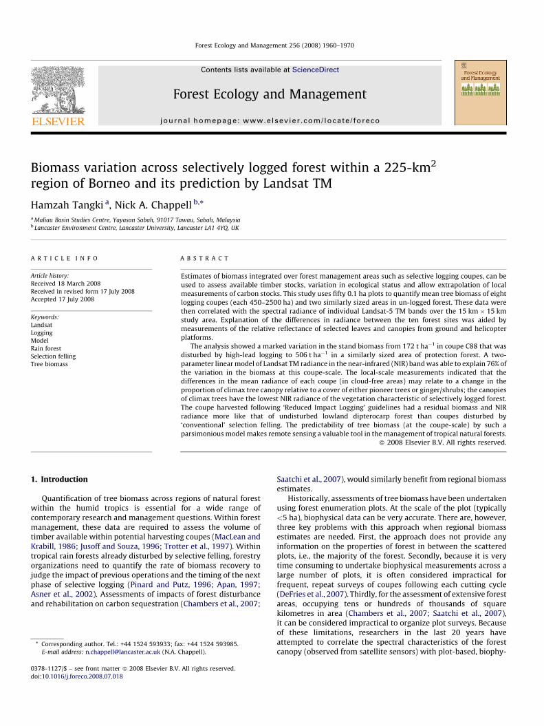
The 225 km2 study region is located within the Ulu SegamaForest Reserve and is managed by the state organization called‘Yayasan Sabah’ for research, education and commercial timberproduction. The area is covered by lowland diperocarp forest,which has an upper and emergent canopy dominated by the familyDipterocarpaceae (Whitmore, 1990). It is the most extensive foresttype in Borneo (Newbery et al., 1992). The annual harvestingcoupes were logged by selection felling in years: 1981 (Coupe1981, or ‘C81’), 1982 (Coupe 1982, or ‘C82’), 1983 (Coupe 1983, or‘C83’), 1988 (Coupe 1988, or ‘C88’), 1989 (Coupe 1989, or ‘C89’),1992 (Coupe 1992, or ‘C92’), and 1993 by conventional selectivefelling (‘C93c’) and Reduced Impact Logging methods (‘C93RIL’).The region also includes undisturbed forest of the water catchmentarea of the Danum Valley Field Centre (DVFC), and a small corner ofthe 438 km2 Danum Valley Conservation Area (DVCA or CONS). TheC81, C82, C83, C88 and C89 coupes were logged using acombination of tractor and high-lead harvesting techniques. With‘high-lead yarding’ (see Conway, 1982) a series of cables radiatefrom a central spar-pole. Each felled tree is then attached to one ofthese cables and winched to the central collecting point; this leavesan area of approximately 20 ha around the spar-pole with few orno trees. This contrasts with the C92, C93c and C93RIL coupes,which were logged using tractor logging alone. Further, the C93RILcoupe was harvested using local Reduced Impact Logging (RIL)guidelines (Pinard et al., 1995; Putz and Pinard, 1993; SabahForestry Department, 1998). These rules aim to minimize collateraldamage to the forest during selection felling to help maintainsustainable timber yields (Pinard and Putz, 1996) and reduceenvironmental impacts (Chappell and Thang, 2007). Selectionfelling within all logging coupes was restricted to only commercialtrees with a diameter breast height (dbh) greater than 60 cm.Moura-Costa and Karolus (1992) and Rakyat Bejaya Sdn. Bhd(1992) collated the timber volumes extracted from each coupeduring the logging operations, and these are presented in Table 1.Coupes C82, C83, and some of C88 were subject to forestrehabilitation, which involved the planting of indigenous treesfrom 1992 onwards. This ‘enrichment planting’ involved fieldmaintenance (e.g., slashing weeds around the line planting) duringthe first to the three years after tree planting at 3–6 monthintervals.

The physiography of the 225 km2 study region is one of ruggedterrain at moderate elevation. The terrain consists of a series ofsteep ridges, with approximately 75% of the area occurring onslopes exceeding 208 that are generally more than 200–300 m long(Pinard, 1995). Annual rainfall recorded at the Danum Valley FieldCentre (DVFC) within the centre of the study area is 2799 mm(1986–2005).

3. Methods

The methodology involved the establishment and measure-ment of fifty 0.1 ha forest plots, sub-sampling of corrected LandsatTM data and subsequent averaging of spectral properties within

H. Tangki, N.A. Chappell / Forest Ecology and Management 256 (2008) 1960–19701962

cloud-free areas of each logging coupe, and the observation of thespectral properties of selected canopies and leaves using a MiltonMultiband Radiometer.

3.1. Plot measurement of tree biophysical data

Tree identification and measurement was undertaken byestablishing 50 plots, each 0.1 ha in area (Figs. 1 and 2; Table 1).Each of the 10 regions studied contained 5 plots based on aconcentric circular design. With this plot design, the smallest/innercircle (radius 2 m) was for the measurement of ‘regeneration

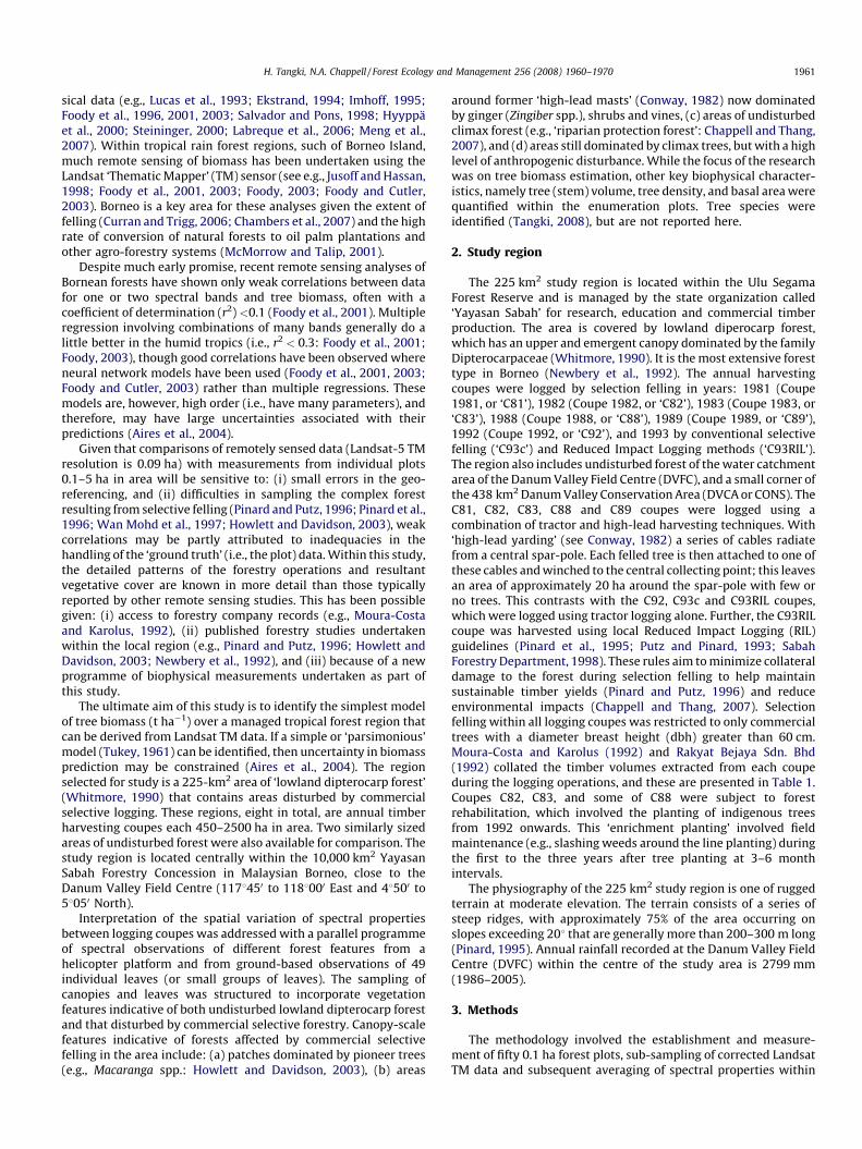
Table 1Details of the logging coupes and protected forest areas within the 225 km2 study reg

Coupes Code Approximated

total area (ha)

Sampling plots

Plot Terrai

slope

Danum Valley Conservation Area CONS 48 000 1 �20

2 �10

3 �10

4 �12

5 �30

Water Catchment Area CATCH 1 000 1 0

2 �5

3 �31

4 �30

5 �12

Reduced Impact Logging Project C93RIL 450 1 �3

2 �26

3 �30

4 �26

5 �20

Conventional Area YL2/93 C93c 1 945 1 �30

2 �40

3 �20

4 �23

5 �20

Coupe 1992 C92 2 500 1 �30

2 �19

3 �21

4 �28

5 �34

Coupe 1989 C89 2 280 1 �13

2 �28

3 �2

4 �18

5 �28

Coupe 1988 C88 2 262 1 �12

2 �10

3 �35

4 �10

5 �26

Coupe 1983 C83 996 1 �20

2 �10

3 �17

4 �12

5 �5

Coupe 1982 C82 2 073 1 �18

2 �20

3 �20

4 �30

5 �35

Coupe 1981 C81 1 637 1 �15

2 �25

3 �17

4 �19

5 �23

Data source was Moura-Costa and Karolus (1992), except for * which refers to Pinard

seedlings’ (below 2 cm dbh at 1.3 m height). In the next circle(radius 12.61 m) all saplings and poles with 2 to 20 cm dbh weremeasured. In the large outer circle (radius 17.84 m or 0.1 ha) alltrees larger than 20 cm dbh were measured. Sanden (1997)reported that using a concentric sample plot design in his studyallowed compensation for a decreasing numerical density with anincreasing diameter and height of trees. Each plot was locatedrandomly within each coupe. Within each plot, tree species wereidentified and measurements of the diameter at breast height(dbh), stem height (for trees with a dbh � 20 cm), and tree locationwithin the plot recorded (Tangki, 2008). The dbh was undertaken

ion, Malaysian Borneo

Logging information

n Year of started

logging

Block Logging

technique

Approximated mean

volume extracted (m3 ha�1)

– – –

– – –

– – – –

– – –

– – –

– – –

– – –

– – – –

– – –

– – –

1993 35 Tractor 87–175*

37

34

29

29

1993 24 Tractor 68**

23

24

25

24

1992 96 Tractor 115**

83

114

86

71

1989 56 High-lead 100

52

9

58

67

1988 5 Tractor 96

10 Tractor

43 High-lead

60 Tractor

23 Tractor

1983 9 Tractor 122

25

15

13

29

1982 1 Tractor 126

41 Tractor

46 High-lead

56 High-lead

2 High-lead

1981 46 Tractor 81

30 High-lead

21 Tractor

80 Tractor

4 Tractor

(1995) and ** Rakyat Bejaya Sdn. Bhd (1992).

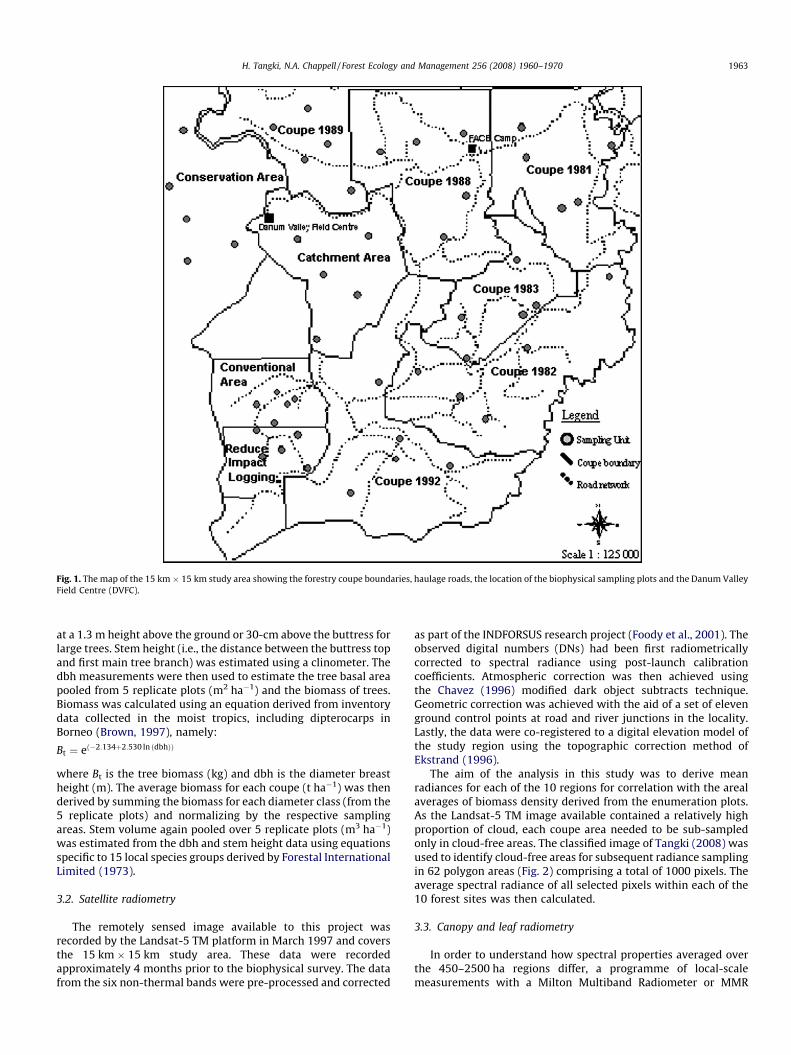
Fig. 1. The map of the 15 km � 15 km study area showing the forestry coupe boundaries, haulage roads, the location of the biophysical sampling plots and the Danum Valley

Field Centre (DVFC).


at a 1.3 m height above the ground or 30-cm above the buttress forlarge trees. Stem height (i.e., the distance between the buttress topand first main tree branch) was estimated using a clinometer. Thedbh measurements were then used to estimate the tree basal areapooled from 5 replicate plots (m2 ha�1) and the biomass of trees.Biomass was calculated using an equation derived from inventorydata collected in the moist tropics, including dipterocarps inBorneo (Brown, 1997), namely:

Bt ¼ eð�2:134þ2:530 ln ðdbhÞÞ

where Bt is the tree biomass (kg) and dbh is the diameter breastheight (m). The average biomass for each coupe (t ha�1) was thenderived by summing the biomass for each diameter class (from the5 replicate plots) and normalizing by the respective samplingareas. Stem volume again pooled over 5 replicate plots (m3 ha�1)was estimated from the dbh and stem height data using equationsspecific to 15 local species groups derived by Forestal InternationalLimited (1973).

3.2. Satellite radiometry

The remotely sensed image available to this project wasrecorded by the Landsat-5 TM platform in March 1997 and coversthe 15 km � 15 km study area. These data were recordedapproximately 4 months prior to the biophysical survey. The datafrom the six non-thermal bands were pre-processed and corrected

as part of the INDFORSUS research project (Foody et al., 2001). Theobserved digital numbers (DNs) had been first radiometricallycorrected to spectral radiance using post-launch calibrationcoefficients. Atmospheric correction was then achieved usingthe Chavez (1996) modified dark object subtracts technique.Geometric correction was achieved with the aid of a set of elevenground control points at road and river junctions in the locality.Lastly, the data were co-registered to a digital elevation model ofthe study region using the topographic correction method ofEkstrand (1996).

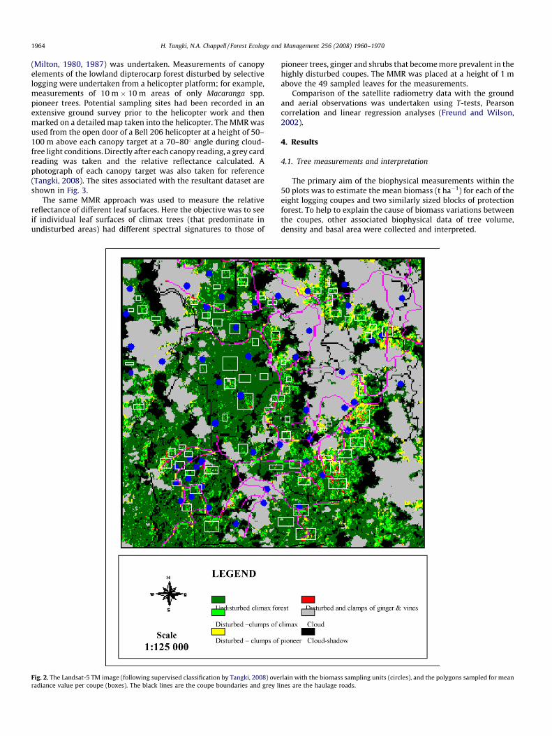
The aim of the analysis in this study was to derive meanradiances for each of the 10 regions for correlation with the arealaverages of biomass density derived from the enumeration plots.As the Landsat-5 TM image available contained a relatively highproportion of cloud, each coupe area needed to be sub-sampledonly in cloud-free areas. The classified image of Tangki (2008) wasused to identify cloud-free areas for subsequent radiance samplingin 62 polygon areas (Fig. 2) comprising a total of 1000 pixels. Theaverage spectral radiance of all selected pixels within each of the10 forest sites was then calculated.

3.3. Canopy and leaf radiometry

In order to understand how spectral properties averaged overthe 450–2500 ha regions differ, a programme of local-scalemeasurements with a Milton Multiband Radiometer or MMR


(Milton, 1980, 1987) was undertaken. Measurements of canopyelements of the lowland dipterocarp forest disturbed by selectivelogging were undertaken from a helicopter platform; for example,measurements of 10 m � 10 m areas of only Macaranga spp.pioneer trees. Potential sampling sites had been recorded in anextensive ground survey prior to the helicopter work and thenmarked on a detailed map taken into the helicopter. The MMR wasused from the open door of a Bell 206 helicopter at a height of 50–100 m above each canopy target at a 70–808 angle during cloud-free light conditions. Directly after each canopy reading, a grey cardreading was taken and the relative reflectance calculated. Aphotograph of each canopy target was also taken for reference(Tangki, 2008). The sites associated with the resultant dataset areshown in Fig. 3.

The same MMR approach was used to measure the relativereflectance of different leaf surfaces. Here the objective was to seeif individual leaf surfaces of climax trees (that predominate inundisturbed areas) had different spectral signatures to those of

Fig. 2. The Landsat-5 TM image (following supervised classification by Tangki, 2008) ove

radiance value per coupe (boxes). The black lines are the coupe boundaries and grey l

pioneer trees, ginger and shrubs that become more prevalent in thehighly disturbed coupes. The MMR was placed at a height of 1 mabove the 49 sampled leaves for the measurements.

Comparison of the satellite radiometry data with the groundand aerial observations was undertaken using T-tests, Pearsoncorrelation and linear regression analyses (Freund and Wilson,2002).

4. Results

4.1. Tree measurements and interpretation

The primary aim of the biophysical measurements within the50 plots was to estimate the mean biomass (t ha�1) for each of theeight logging coupes and two similarly sized blocks of protectionforest. To help to explain the cause of biomass variations betweenthe coupes, other associated biophysical data of tree volume,density and basal area were collected and interpreted.

rlain with the biomass sampling units (circles), and the polygons sampled for mean

ines are the haulage roads.

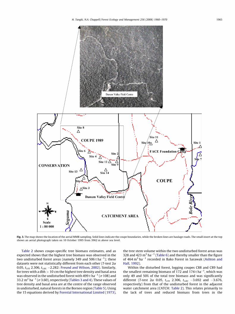
Fig. 3. The map shows the location of the aerial MMR sampling. Solid lines indicate the coupe boundaries, while the broken lines are haulage roads. The small insert at the top

shows an aerial photograph taken on 10 October 1995 from 3962 m above sea level.


Table 2 shows coupe-specific tree biomass estimates, and asexpected shows that the highest tree biomass was observed in thetwo undisturbed forest areas (namely 349 and 506 t ha�1); thesedatasets were not statistically different from each other (T-test 2a0.05, tcrit 2.306, tcalc �2.282: Freund and Wilson, 2002). Similarly,for trees with a dbh > 10 cm the highest tree density and basal areawas observed in the undisturbed forest with 499 t ha�1 (s 108) and33.2 m2 ha�1 (s 3.60), respectively (Tables 3 and 4). These values oftree density and basal area are at the centre of the range observedin undisturbed, natural forests in the Borneo region (Table 5). Usingthe 15 equations derived by Forestal International Limited (1973),

the tree stem volume within the two undisturbed forest areas was328 and 423 m3 ha�1 (Table 6) and thereby smaller than the figureof 464 m3 ha�1 recorded in Bako Forest in Sarawak (Ashton andHall, 1992).

Within the disturbed forest, logging coupes C88 and C89 hadthe smallest remaining biomass of 172 and 174 t ha�1, which wasonly 49 and 50% of the total tree biomass and was significantlydifferent (T-test 2a 0.05, tcrit 2.306, tcalc �3.692 and �3.676,respectively) from that of the undisturbed forest in the adjacentwater catchment area (CATCH: Table 2). This relates primarily tothe lack of trees and reduced biomass from trees in the

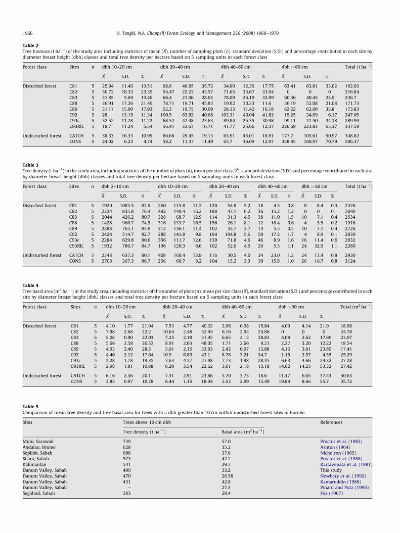
Table 2Tree biomass (t ha�1) of the study area including statistics of mean (X), number of sampling plots (n), standard deviation (S.D.) and percentage contributed in each site by

diameter breast height (dbh) classes and total tree density per hectare based on 5 sampling units in each forest class

Forest class Sites n dbh 10–20 cm dbh 20–40 cm dbh 40–60 cm dbh > 60 cm Total (t ha�1)

X S.D. % X S.D. % X S.D. % X S.D. %

Disturbed forest C81 5 25.94 11.49 13.51 68.6 46.85 35.72 34.09 12.36 17.75 63.41 63.81 33.02 192.03

C82 5 50.72 18.33 23.39 94.47 22.23 43.57 71.65 35.67 33.04 0 0 0 216.84

C83 5 31.85 5.69 13.46 66.4 21.06 28.05 78.09 26.19 32.99 60.36 40.45 25.5 236.7

C88 5 36.91 17.26 21.49 78.71 19.71 45.83 19.92 30.23 11.6 36.19 52.08 21.08 171.73

C89 5 31.17 15.90 17.93 52.3 19.75 30.09 28.13 11.42 16.18 62.22 62.00 35.8 173.83

C92 5 28 13.15 11.34 100.5 63.82 40.68 103.31 40.04 41.82 15.25 34.09 6.17 247.05

C93c 5 32.52 11.28 11.22 68.52 42.48 23.63 89.84 25.35 30.98 99.11 72.50 34.18 289.99

C93RIL 5 18.7 11.24 5.54 56.41 32.67 16.71 41.77 25.66 12.37 220.69 223.83 65.37 337.58

Undisturbed forest CATCH 5 38.33 16.33 10.99 66.68 29.45 19.13 65.91 43.01 18.91 177.7 105.61 50.97 348.62

CONS 5 24.02 6.23 4.74 58.2 11.37 11.49 65.7 36.09 12.97 358.45 160.97 70.79 506.37

Table 3Tree density (t ha�1) in the study area, including statistics of the number of plots (n), mean per size class (X), standard deviation (S.D.) and percentage contributed in each site

by diameter breast height (dbh) classes and total tree density per hectare based on 5 sampling units in each forest class

Forest class Sites n dbh 2–10 cm dbh 10–20 cm dbh 20–40 cm dbh 40–60 cm dbh > 60 cm Total (t ha�1)

X S.D. % X S.D. % X S.D. % X S.D. % X S.D. %

Disturbed forest C81 5 1920 1083.5 82.5 260 115.8 11.2 120 54.8 5.2 18 4.5 0.8 8 8.4 0.3 2326

C82 5 2324 835.8 76.4 492 140.4 16.2 188 47.1 6.2 36 15.2 1.2 0 0 0 3040

C83 5 2044 426.2 80.7 328 68.7 12.9 114 31.3 4.5 38 11.0 1.5 10 7.1 0.4 2534

C88 5 1428 960.7 74.5 316 133.7 16.5 156 26.1 8.1 12 16.4 0.6 4 5.5 0.2 1916

C89 5 2288 765.1 83.9 312 136.1 11.4 102 32.7 3.7 14 5.5 0.5 10 7.1 0.4 2726

C92 5 2424 514.7 82.7 288 141.8 9.8 164 104.8 5.6 50 17.3 1.7 4 8.9 0.1 2930

C93c 5 2284 629.8 80.6 356 111.7 12.6 130 71.8 4.6 46 8.9 1.6 16 11.4 0.6 2832

C93RIL 5 1932 786.7 84.7 196 120.3 8.6 102 52.6 4.5 26 5.5 1.1 24 32.9 1.1 2280

Undisturbed forest CATCH 5 2348 637.3 80.1 408 160.4 13.9 116 30.5 4.0 34 23.0 1.2 24 13.4 0.8 2930

CONS 5 2708 367.3 86.7 256 60.7 8.2 104 15.2 3.3 30 15.8 1.0 26 16.7 0.8 3124

Table 4Tree basal area (m2 ha�1) in the study area, including statistics of the number of plots (n), mean per size class (X), standard deviation (S.D.) and percentage contributed in each

site by diameter breast height (dbh) classes and total tree density per hectare based on 5 sampling units in each forest class

Forest class Sites n dbh 10–20 cm dbh 20–40 cm dbh 40–60 cm dbh >60 cm Total (m2 ha�1)

X S.D. % X S.D. % X S.D. % X S.D. %

Disturbed forest C81 5 4.10 1.77 21.94 7.53 4.77 40.32 2.96 0.98 15.84 4.09 4.14 21.9 18.68

C82 5 7.98 2.68 32.2 10.64 2.48 42.94 6.16 2.94 24.86 0 0 0 24.78

C83 5 5.08 0.90 22.03 7.25 2.18 31.45 6.65 2.13 28.83 4.08 2.62 17.69 23.07

C88 5 5.66 2.58 30.52 8.91 2.03 48.05 1.71 2.66 9.21 2.27 3.20 12.22 18.54

C89 5 4.93 2.40 28.3 5.91 2.15 33.93 2.42 0.97 13.88 4.16 3.81 23.89 17.41

C92 5 4.46 2.12 17.64 10.9 6.89 43.1 8.78 3.21 34.7 1.15 2.57 4.55 25.29

C93c 5 5.28 1.78 19.35 7.63 4.57 27.98 7.73 1.98 28.35 6.63 4.66 24.32 27.28

C93RIL 5 2.98 1.81 10.88 6.20 3.54 22.62 3.61 2.18 13.18 14.62 14.23 53.32 27.42


CONS 5 3.85 0.97 10.78 6.44 1.15 18.04 5.53 2.99 15.49 19.89 8.66 55.7 35.72

Table 5Comparison of mean tree density and tree basal area for trees with a dbh greater than 10 cm within undisturbed forest sites in Borneo

Sites Trees above 10 cm dbh References

Tree density (t ha�1) Basal area (m2 ha�1)

Mulu, Sarawak 739 57.0 Proctor et al. (1983)

Andalau, Brunei 628 35.2 Ashton (1964)

Sepilok, Sabah 608 37.8 Nicholson (1965)

Silam, Sabah 573 42.2 Proctor et al. (1988)

Kalimantan 541 29.7 Kartawinata et al. (1981)

Danum Valley, Sabah 499 33.2 This study

Danum Valley, Sabah 470 26.58 Newbery et al. (1992)

Danum Valley, Sabah 431 42.8 Kamaruddin (1986)

Danum Valley, Sabah – 27.5 Pinard and Putz (1996)

Segaliud, Sabah 283 28.4 Fox (1967)


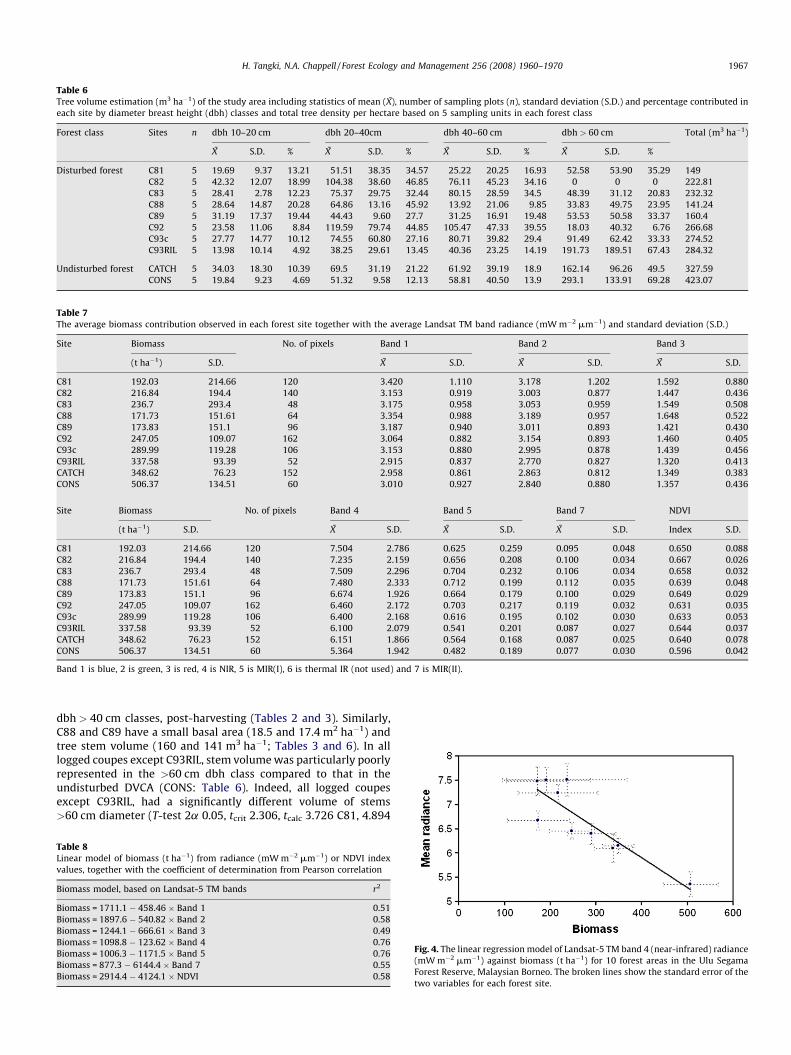
Table 6Tree volume estimation (m3 ha�1) of the study area including statistics of mean (X), number of sampling plots (n), standard deviation (S.D.) and percentage contributed in

each site by diameter breast height (dbh) classes and total tree density per hectare based on 5 sampling units in each forest class

Forest class Sites n dbh 10–20 cm dbh 20–40cm dbh 40–60 cm dbh > 60 cm Total (m3 ha�1)

X S.D. % X S.D. % X S.D. % X S.D. %

Disturbed forest C81 5 19.69 9.37 13.21 51.51 38.35 34.57 25.22 20.25 16.93 52.58 53.90 35.29 149

C82 5 42.32 12.07 18.99 104.38 38.60 46.85 76.11 45.23 34.16 0 0 0 222.81

C83 5 28.41 2.78 12.23 75.37 29.75 32.44 80.15 28.59 34.5 48.39 31.12 20.83 232.32

C88 5 28.64 14.87 20.28 64.86 13.16 45.92 13.92 21.06 9.85 33.83 49.75 23.95 141.24

C89 5 31.19 17.37 19.44 44.43 9.60 27.7 31.25 16.91 19.48 53.53 50.58 33.37 160.4

C92 5 23.58 11.06 8.84 119.59 79.74 44.85 105.47 47.33 39.55 18.03 40.32 6.76 266.68

C93c 5 27.77 14.77 10.12 74.55 60.80 27.16 80.71 39.82 29.4 91.49 62.42 33.33 274.52

C93RIL 5 13.98 10.14 4.92 38.25 29.61 13.45 40.36 23.25 14.19 191.73 189.51 67.43 284.32


CONS 5 19.84 9.23 4.69 51.32 9.58 12.13 58.81 40.50 13.9 293.1 133.91 69.28 423.07

Table 7The average biomass contribution observed in each forest site together with the average Landsat TM band radiance (mW m�2 mm�1) and standard deviation (S.D.)

Site Biomass No. of pixels Band 1 Band 2 Band 3

(t ha�1) S.D. X S.D. X S.D. X S.D.

C81 192.03 214.66 120 3.420 1.110 3.178 1.202 1.592 0.880

C82 216.84 194.4 140 3.153 0.919 3.003 0.877 1.447 0.436

C83 236.7 293.4 48 3.175 0.958 3.053 0.959 1.549 0.508

C88 171.73 151.61 64 3.354 0.988 3.189 0.957 1.648 0.522

C89 173.83 151.1 96 3.187 0.940 3.011 0.893 1.421 0.430

C92 247.05 109.07 162 3.064 0.882 3.154 0.893 1.460 0.405

C93c 289.99 119.28 106 3.153 0.880 2.995 0.878 1.439 0.456

C93RIL 337.58 93.39 52 2.915 0.837 2.770 0.827 1.320 0.413

CATCH 348.62 76.23 152 2.958 0.861 2.863 0.812 1.349 0.383

CONS 506.37 134.51 60 3.010 0.927 2.840 0.880 1.357 0.436

Site Biomass No. of pixels Band 4 Band 5 Band 7 NDVI

(t ha�1) S.D. X S.D. X S.D. X S.D. Index S.D.

C81 192.03 214.66 120 7.504 2.786 0.625 0.259 0.095 0.048 0.650 0.088

C82 216.84 194.4 140 7.235 2.159 0.656 0.208 0.100 0.034 0.667 0.026

C83 236.7 293.4 48 7.509 2.296 0.704 0.232 0.106 0.034 0.658 0.032

C88 171.73 151.61 64 7.480 2.333 0.712 0.199 0.112 0.035 0.639 0.048

C89 173.83 151.1 96 6.674 1.926 0.664 0.179 0.100 0.029 0.649 0.029

C92 247.05 109.07 162 6.460 2.172 0.703 0.217 0.119 0.032 0.631 0.035

C93c 289.99 119.28 106 6.400 2.168 0.616 0.195 0.102 0.030 0.633 0.053

C93RIL 337.58 93.39 52 6.100 2.079 0.541 0.201 0.087 0.027 0.644 0.037

CATCH 348.62 76.23 152 6.151 1.866 0.564 0.168 0.087 0.025 0.640 0.078

CONS 506.37 134.51 60 5.364 1.942 0.482 0.189 0.077 0.030 0.596 0.042

Band 1 is blue, 2 is green, 3 is red, 4 is NIR, 5 is MIR(I), 6 is thermal IR (not used) and 7 is MIR(II).


dbh > 40 cm classes, post-harvesting (Tables 2 and 3). Similarly,C88 and C89 have a small basal area (18.5 and 17.4 m2 ha�1) andtree stem volume (160 and 141 m3 ha�1; Tables 3 and 6). In alllogged coupes except C93RIL, stem volume was particularly poorlyrepresented in the >60 cm dbh class compared to that in theundisturbed DVCA (CONS: Table 6). Indeed, all logged coupesexcept C93RIL, had a significantly different volume of stems>60 cm diameter (T-test 2a 0.05, tcrit 2.306, tcalc 3.726 C81, 4.894

Table 8Linear model of biomass (t ha�1) from radiance (mW m�2 mm�1) or NDVI index

values, together with the coefficient of determination from Pearson correlation

Biomass model, based on Landsat-5 TM bands r2

Biomass = 1711.1 � 458.46 � Band 1 0.51

Biomass = 1897.6 � 540.82 � Band 2 0.58

Biomass = 1244.1 � 666.61 � Band 3 0.49

Biomass = 1098.8 � 123.62 � Band 4 0.76

Biomass = 1006.3 � 1171.5 � Band 5 0.76

Biomass = 877.3 � 6144.4 � Band 7 0.55

Biomass = 2914.4 � 4124.1 � NDVI 0.58

Fig. 4. The linear regression model of Landsat-5 TM band 4 (near-infrared) radiance

(mW m�2 mm�1) against biomass (t ha�1) for 10 forest areas in the Ulu Segama

Forest Reserve, Malaysian Borneo. The broken lines show the standard error of the

two variables for each forest site.

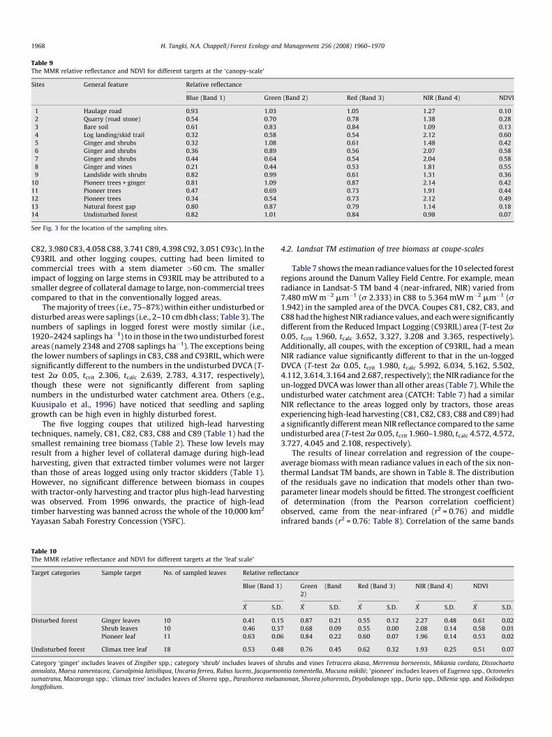
Table 9The MMR relative reflectance and NDVI for different targets at the ‘canopy-scale’

Sites General feature Relative reflectance

Blue (Band 1) Green (Band 2) Red (Band 3) NIR (Band 4) NDVI

1 Haulage road 0.93 1.03 1.05 1.27 0.10

2 Quarry (road stone) 0.54 0.70 0.78 1.38 0.28

3 Bare soil 0.61 0.83 0.84 1.09 0.13

4 Log landing/skid trail 0.32 0.58 0.54 2.12 0.60

5 Ginger and shrubs 0.32 1.08 0.61 1.48 0.42



8 Ginger and vines 0.21 0.44 0.53 1.81 0.55

9 Landslide with shrubs 0.82 0.99 0.61 1.31 0.36

10 Pioneer trees + ginger 0.81 1.09 0.87 2.14 0.42

11 Pioneer trees 0.47 0.69 0.73 1.91 0.44

12 Pioneer trees 0.34 0.54 0.73 2.12 0.49

13 Natural forest gap 0.80 0.87 0.79 1.14 0.18

14 Undisturbed forest 0.82 1.01 0.84 0.98 0.07

See Fig. 3 for the location of the sampling sites.


C82, 3.980 C83, 4.058 C88, 3.741 C89, 4.398 C92, 3.051 C93c). In theC93RIL and other logging coupes, cutting had been limited tocommercial trees with a stem diameter >60 cm. The smallerimpact of logging on large stems in C93RIL may be attributed to asmaller degree of collateral damage to large, non-commercial treescompared to that in the conventionally logged areas.

The majority of trees (i.e., 75–87%) within either undisturbed ordisturbed areas were saplings (i.e., 2–10 cm dbh class; Table 3). Thenumbers of saplings in logged forest were mostly similar (i.e.,1920–2424 saplings ha�1) to in those in the two undisturbed forestareas (namely 2348 and 2708 saplings ha�1). The exceptions beingthe lower numbers of saplings in C83, C88 and C93RIL, which weresignificantly different to the numbers in the undisturbed DVCA (T-test 2a 0.05, tcrit 2.306, tcalc 2.639, 2.783, 4.317, respectively),though these were not significantly different from saplingnumbers in the undisturbed water catchment area. Others (e.g.,Kuusipalo et al., 1996) have noticed that seedling and saplinggrowth can be high even in highly disturbed forest.

The five logging coupes that utilized high-lead harvestingtechniques, namely, C81, C82, C83, C88 and C89 (Table 1) had thesmallest remaining tree biomass (Table 2). These low levels mayresult from a higher level of collateral damage during high-leadharvesting, given that extracted timber volumes were not largerthan those of areas logged using only tractor skidders (Table 1).However, no significant difference between biomass in coupeswith tractor-only harvesting and tractor plus high-lead harvestingwas observed. From 1996 onwards, the practice of high-leadtimber harvesting was banned across the whole of the 10,000 km2

Yayasan Sabah Forestry Concession (YSFC).

Table 10The MMR relative reflectance and NDVI for different targets at the ‘leaf scale’

Target categories Sample target No. of sampled leaves Relative refle

Blue (Band 1

X S.D

Disturbed forest Ginger leaves 10 0.41 0.1

Shrub leaves 10 0.46 0.3

Pioneer leaf 11 0.63 0.0

Undisturbed forest Climax tree leaf 18 0.53 0.4

Category ‘ginger’ includes leaves of Zingiber spp.; category ‘shrub’ includes leaves of sh

annulata, Maesa ramentacea, Caesalpinia latisiliqua, Uncaria ferrea, Rubus lucens, Jacquemo

sumatrana, Macaranga spp.; ‘climax tree’ includes leaves of Shorea spp., Parashorea melaa

longifolium.

4.2. Landsat TM estimation of tree biomass at coupe-scales

Table 7 shows the mean radiance values for the 10 selected forestregions around the Danum Valley Field Centre. For example, meanradiance in Landsat-5 TM band 4 (near-infrared, NIR) varied from7.480 mW m�2 mm�1 (s 2.333) in C88 to 5.364 mW m�2 mm�1 (s1.942) in the sampled area of the DVCA. Coupes C81, C82, C83, andC88 had the highest NIR radiance values, and each were significantlydifferent from the Reduced Impact Logging (C93RIL) area (T-test 2a0.05, tcrit 1.960, tcalc 3.652, 3.327, 3.208 and 3.365, respectively).Additionally, all coupes, with the exception of C93RIL, had a meanNIR radiance value significantly different to that in the un-loggedDVCA (T-test 2a 0.05, tcrit 1.980, tcalc 5.992, 6.034, 5.162, 5.502,4.112, 3.614, 3.164 and 2.687, respectively); the NIR radiance for theun-logged DVCA was lower than all other areas (Table 7). While theundisturbed water catchment area (CATCH: Table 7) had a similarNIR reflectance to the areas logged only by tractors, those areasexperiencing high-lead harvesting (C81, C82, C83, C88 and C89) hada significantly different mean NIR reflectance compared to the sameundisturbed area (T-test 2a 0.05, tcrit 1.960–1.980, tcalc 4.572, 4.572,3.727, 4.045 and 2.108, respectively).

The results of linear correlation and regression of the coupe-average biomass with mean radiance values in each of the six non-thermal Landsat TM bands, are shown in Table 8. The distributionof the residuals gave no indication that models other than two-parameter linear models should be fitted. The strongest coefficientof determination (from the Pearson correlation coefficient)observed, came from the near-infrared (r2 = 0.76) and middleinfrared bands (r2 = 0.76: Table 8). Correlation of the same bands

ctance

) Green (Band

2)

Red (Band 3) NIR (Band 4) NDVI

. X S.D. X S.D. X S.D. X S.D.

5 0.87 0.21 0.55 0.12 2.27 0.48 0.61 0.02

7 0.68 0.09 0.55 0.00 2.08 0.14 0.58 0.01

6 0.84 0.22 0.60 0.07 1.96 0.14 0.53 0.02

8 0.76 0.45 0.62 0.32 1.93 0.25 0.51 0.07

rubs and vines Tetracera akasa, Merremia borneensis, Mikania cordata, Dissochaeta

ntia tomentella, Mucuna mikilii; ‘pioneer’ includes leaves of Eugenea spp., Octomeles

nonan, Shorea johorensis, Dryobalanops spp., Durio spp., Dillenia spp. and Koilodepas


with the coupe-average, stem volume gave an equally highcoefficient of determination for the near-infrared band (r2 = 0.75),but a much weaker strength of association in the middle infraredband (i.e., r2 = 0.44). Explanation of �75% of biomass and stemvolume variations between areas the size of logging coupes (i.e.,450–2500 ha) with the NIR spectral signature alone, was muchgreater than that produced by single spectral bands previouslyexamined for the area (see e.g., Foody et al., 2001). The smallnumber of samples (10 sites) means that the statistical significanceof the regression model cannot be calculated. The standard error ofeach variable, therefore, is shown in Fig. 4 as a visual estimate ofthe uncertainty. Others have sought to improve the strength of theradiance-biomass correlation by combining different spectralbands, but this can have the negative effect of increasing theuncertainty in the model further (Aires et al., 2004). Indeed,combining the NIR values with band 3 (red) values in theNormalized Difference Vegetation Index (NDVI) produced a muchlower strength of correlation within this study (Table 8).

The preliminary NIR-based biomass model, we call the nirBmodel, is expressed as:

Ba ¼ 1098:8� 123:64 ðNIRÞ; r2 ¼ 0:76

where Ba is the mean biomass of a 450–2500 ha area of lowlanddipterocarp forest (t ha�1) and NIR is the Landsat TM near-infraredradiance for vegetation canopies unaffected by cloud(mW m�2 mm�1). The preliminary model indicates that the coupecut by RIL methods (C93RIL) had a greater residual biomasscompared to the other logging coupes (Table 7; Fig. 4), particularlythose incorporating high-lead logging, despite having a similarlyhigh extraction volume (Table 1). Indeed, the mean biomass andNIR radiance of the RIL area looks more like undisturbed forestthan conventionally logged forest (Fig. 4).

4.3. Interpretation of the radiance-biomass association using sub-

coupe radiometry

The helicopter-based radiometry of selected 0.01 ha canopyareas (Table 9) indicated that the highest relative reflectance in theNIR band was observed for areas dominated by either ginger/shrubs (1.31–2.07) or pioneer tree canopies (1.91–2.14). Incontrast, the canopy of undisturbed climax trees had the lowestrelative reflectance in the NIR band (0.98) for vegetated areas(Table 9).

Examination of the spectral signature of individual leaves (orsmall groups of leaves) in the NIR band gave similar results. Thehighest relative reflectance in the NIR band was observed forginger and shrub leaves (2.08–2.27) or pioneer tree leaves (1.96).The lowest NIR reflectance was for the leaves of climax trees (1.93:Table 10), and this was significantly different from that of gingerleaves (T-test 2a 0.05, tcrit 2.056, tcalc�2.088), but not for the shrubor pioneer tree leaves. While the relative importance of ginger/shrubs or pioneer trees to NIR reflectance seems to depend on scale(Tables 9 and 10), it is clear that leaves and canopies of climax treeshave low NIR reflectance. This finding is consistent with the coupe-scale estimates, where undisturbed climax forest has the lowestaverage NIR radiance (i.e., corrected reflectance: Table 7).

5. Extending the work and forest management applications

There are several ways that this research could be extended andapplied to the management of lowland dipterocarp forests. Thesatellite-based technique for biomass estimation in lowlanddipterocarp forest presented here should be extended by validat-ing the nirB model across a much larger distribution of annuallogging coupes of similar forest that have intensively sampled and

high quality forest enumeration data. Such areas may be presentelsewhere within the 10,000 km2 Yayasan Sabah Forestry Con-cession, or elsewhere within Borneo Island.

Even before wider testing is undertaken, the nirB model forlowland dipterocarp forest should be evaluated as part of tropicalforest management. Application of the nirB model to all of theannual coupes within the 10,000 km2 Yayasan Sabah ForestryConcession could be helpful in the assessment of timber stocks,and in the assessment of the ecological status of this large forestedregion (Sinun et al., 2007). Further, application of the nirB model tomore recent Landsat TM data, for example, data collected in 2007following a further 10 years of forest recovery could be beneficial.By differencing the coupe-scale biomass estimates between thetwo periods (e.g., 1997 and 2007) the current rate of forestrecovery can be assessed, including the effects of enrichmentplanting within some of the coupe areas (Moura-Costa et al., 1996).This assessment would be most valuable if the measurements onthe fifty (geo-referenced and tagged) enumeration plots were alsorepeated. Lastly, application of the nirB model to the whole438 km2 Danum Valley Conservation Area would allow apreliminary assessment of the spatial variations in tree biomassacross the DVCA that would help in the planning of futuremanagement options for this protected area (Marsh, 1995).

Following validation of the model and a demonstration of thetechnique’s value to forest management across a large tract offorest, the nirB model could be evaluated in other lowlanddipterocarp forests elsewhere in Borneo or Southeast Asia.

6. Conclusions

This study has demonstrated the considerable potential forestimating tree biomass at the scale of annual logging coupeswithin an area of lowland dipterocarp forest. Considerableopportunities for extending and applying this research withinthe Ulu Segama Forest Reserve or whole Yayasan Sabah ForestryConcession exist, and following validation of the model, to otherareas of lowland dipterocarp forests in Borneo or Southeast Asia.

Acknowledgements

The authors would like to thank the Royal Society of London andYayasan Sabah (particularly Dr. Waidi Sinun) for their financialsupport. We would also like to thank the Malaysian Centre forRemote Sensing (MACRES) and the European Union INDFORSUSproject for the provision of the corrected Landsat-5 TM image. Wegratefully acknowledge the assistance of E.S. Alipp, A. Ratag, S.Dasip, J. Arabin and J. Tarman (of Yayasan Sabah) during thebiophysical survey.

References

Aires, F., Prigent, C., Rossow, W.B., 2004. Neural network uncertainty assessment usingBayesian statistics with application to remote sensing: 1. Network weights.Journal of Geophysical Research 109, D10303, doi:10.1029/2003JD004173.

Apan, A.A., 1997. Land cover mapping for tropical forest rehabilitation planningusing remotely sensed data. International Journal of Remote Sensing 8, 1029–1049.

Ashton, P.S., 1964. Ecological Studies in the Mixed Dipterocarp Forest of BruneiState. Oxford. For. Mem., p. 25.

Ashton, P.S., Hall, P., 1992. Comparison of structure among mixed dipterocarp forestof North-Western Borneo. Journal of Ecology 80, 459–481.

Asner, G.P., Keller, M., Pereira, R., Zweede, J.C., 2002. Remote sensing of selectivelogging in Amazonia assessing limitations based on detailed field observa-tions, Landsat ETM+, and textural analysis. Remote Sensing of Environment80, 483–496.

Brown, S. 1997. Estimating biomass and biomass change of tropical forest. A primerreport, FAO, Rome.

Chambers, J.Q., Asner, G., Morton, D., Anderson, L.O., Saatchi, S., Espırito-Santo, F.D-B., Palace, M., Souza Jr., C., 2007. Regional ecosystem structure and function:

http://dx.doi.org/10.1029/2003JD004173


ecological insights from remote sensing of tropical forests. Trends in Ecologyand Evolution 22, 414–423.

Chappell, N.A., Thang, H.C., 2007. Practical hydrological protection for tropicalnatural forests: the Malaysian experience. Unasylva 229 (58), 17–21.

Chavez, P.S., 1996. Image-based atmospheric corrections—revised and revisited.Photogrammetric Engineering and Remote Sensing 62, 1025–1036.

Conway, S., 1982. Logging Practices. Miller Freeman Publications, San Francisco.Curran, L.M., Trigg, S.N., 2006. Sustainability science from space: quantifying forest

disturbance and land-use dynamics in the Amazon. PNAS 103, 12663–12664.DeFries, R., Achard, F., Brown, S., Herold, M., Murdiyarso, D., Schlamadinger, B., de

Souza Jr., C., 2007. Earth observations for estimating greenhouse gas emissionsfrom deforestation in developing countries. Environmental Science and Policy10, 385–394.

Ekstrand, S., 1994. Assessment of forest damage with Landsat TM: correction forvarying forest stand characteristics. Remote Sensing of Environment 47, 291–302.

Ekstrand, S., 1996. Landsat TM-based forest damage assessment: correction fortopographic effects. Photogrammetric Engineering and Remote Sensing 62,151–161.

Foody, G.M., 2003. Remote sensing of tropical forest environments: towards themonitoring of environmental resources for sustainable development. Interna-tional Journal of Remote Sensing 24, 4035–4046.

Foody, G.M., Cutler, M.E.J., 2003. Tree biodiversity in protected and logged Borneantropical rain forest and it’s measurement by satellite remote sensing. Journal ofBiogeography 30, 1053–1066.

Foody, G.M., Boyd, D.S., Curran, P.J., 1996. Relations between tropical forest bio-physical properties and data acquired in AVHRR channels 1–5. InternationalJournal of Remote Sensing 17, 1341–1355.

Foody, G.M., Cutler, M.E., McMorrow, J., Pelz, D., Tangki, H., Boyd, D.S., 2001.Mapping the biomass of Bornean tropical rain forest from remotely senseddata. Global Ecology and Biogeography 10, 379–387.

Foody, G.M., Boyd, D.S., Cutler, M.E.J., 2003. Predictive relations of tropical forestbiomass from Landsat TM data and their transferability between regions.Remote Sensing of Environment 85, 463–474.

Forestal International Limited. 1973. Sabah Forest Inventory 1969–1972. Volume 1and 1A. Project No. F644/2 April 1973. Vancouver, Canada.

Fox, J.E.D., 1967. An enumeration of lowland dipterocarp forest in Sabah. MalayaForester 30, 263–279.

Freund, R., Wilson, W., 2002. Statistical Methods, second ed. Academic Press, SanDiego.

Howlett, B.E., Davidson, D.W., 2003. Effects of seed availability, site conditions, andherbivory on pioneer recruitment after logging in Sabah. Malaysia ForestEcology and Management 184, 369–383.

Hyyppa, J., Hyyppa, H., Inkinen, M., Engdahl, M., Linko, S., Zhu, Y.H., 2000. Accuracycomparison of various remote sensing data sources in the retrieval of foreststand attributes. Forest Ecology and Management 128, 109–120.

Imhoff, M.L., 1995. Radar backscatter and biomass saturation—ramifications forglobal biomas inventory. IEEE Transactions on Geoscience and Remote Sensing33, 511–518.

Jusoff, K., Souza, G.D., 1996. Use of remote sensing in Malaysia forestry and itspotential. International Journal of Remote Sensing 18, 57–70.

Jusoff, K., Hassan, H.M., 1998. An overview of satellite remote sensing for landuseplanning with special emphasis in Malaysia. Remote Sensing Review 16, 209–231.

Kamaruddin, I. 1986. Structure and species composition of lowland dipterocarpforest in Danum Valley. B.Sc. Thesis. University Kebangsaan Malaysia, Sabah.Unpublished.

Kartawinata, K., Abdulhadi, Partomihardjo, T., 1981. Composition and structure of alowland dipterocarp forest at Wanariest, East Kalimantan. Malaya Forester 44,307–406.

Kuusipalo, J., Jafarsidik, Y., Adjers, G., Tuomela, K., 1996. Population dynamics of treeseedlings in mixed dipterocarp rainforest before and after logging and crownliberation. Forest Ecology and Management 81, 85–94.

Labreque, S., Fournier, R.A., Luther, J.E., Piercey, D., 2006. A comparison of fourmethods to map biomass from Landsat-TM and inventory data in westernNewfoundland. Forest Ecology and Management 226, 129–144.

Lucas, R.M., Honzak, M., Foody, G.M., Curran, P.J., Corves, C., 1993. Characterisingtropical secondary forests using multi-temporal Landsat sensor imagery. Inter-national Journal of Remote Sensing 14, 3061–3067.

MacLean, G.A., Krabill, W.B., 1986. Gross-merchantable timber volume estimationusing an airborne LiDAR system. Canadian Journal of Remote Sensing 12, 7–18.

Marsh, C.W., 1995. Management Plan (1995–2000): Danum Valley ConservationArea, Sabah Malaysia. Sabah/Innoprise Corporation Sdn. Bhd, Kota Kinabalu,Yayasan.

McMorrow, J.M., Talip, Mustapa Abd, 2001. Decline of forest area in Sabah, Malay-sia: relationship to state policies, land code and land capability. Global Envir-onmental Change: Human and Policy Dimensions 11, 217–230.

Meng, Q., Cieszewski, C.J., Madden, M., Borders, B., 2007. A linear mixed-effectsmodel of biomass and volume of trees using Landsat ETM+ images. ForestEcology and Management 244, 93–101.

Milton, E.J., 1980. A portable multiband radiometer for ground data collection inremote sensing. International Journal of Remote Sensing 1, 153–165.

Milton, E.J., 1987. Principle of field spectroscopy. International Journal of RemoteSensing 8, 1807–1827.

Moura-Costa, P., Karolus, A. 1992. Timber extraction volumes (1970–1991) of UluSegama Forest Reserve. Innoprise Corporation Sdn. Bhd. Unpublished.

Moura-Costa, P.H., Yap, S.W., Ong, C.L., Ganing, A., Nussbaum, R., Mojiun, T., 1996.Large scale enrichment planting with dipterocarps as an alternative for carbonoffset—methods and preliminary results. In: Appanah, S., Khoo, K.C. (Eds.), Pro-ceedings of the Fifth Round Table Conference on Dipterocarps, Chiang Mai,Thailand, November 1994. Forest Research Institute of Malaysia (FRIM),Kepong, pp. 386–396.

Newbery, D.McC., Campbell, E.J.F., Lee, Y.F., Ridsdale, C.E., Still, M.J., 1992. Primarylowland dipterocarp forest at Danum Valley, Sabah, Malaysia: structure, rela-tive abundance and family composition. Philosophical Transactions of the RoyalSociety, Series B 335, 341–356.

Nicholson, D.I., 1965. A study of virgin forest near Sandakan North Borneo. In:Proceedings of the Symposium on Ecological Research in Humid TropicalVegetation, Kuching: UNESCO & Government of Sarawak, pp. 67–86.

Pinard, M.A. 1995. Carbon retention by reduced-impact logging. Ph.D. dissertation.University of Florida, Gainesville, Florida.

Pinard, M.A., Putz, F.E., 1996. Retaining forest biomass by reducing logging damage.Biotropica 28, 278–295.

Pinard, M.A., Putz, F.E., Tay, J., Sullivan, T.E., 1995. Creating timber harbest guide-lines for a reduced-impact logging project in Malaysia. Journal of Forestry 93,41–45.

Pinard, M., Howlett, B., Davidson, D.W., 1996. Site conditions limit pioneer treeestablishment after logging of dipterocarp forests in Sabah, Malaysia. Biotropica28, 2–12.

Proctor, J., Anderson, J.M., Chai, P., Vallack, H.W., 1983. Ecological studies in fourcontrasting lowland rain forest in Gunung Mulu National Park, Sarawak. I.Forest environment, structure and floristic. Journal of Ecology 71, 237–260.

Proctor, J., Lee, Y.F., Langley, A.M., Munro, W.R.C., Nelson, T., 1988. Ecological studieson Gunung Silam, a small ultrabasic mountain in Sabah, Malaysia. I. Environ-ment, forest structure and floristics. Journal of Ecology 76, 320–340.

Putz, F.E., Pinard, 1993. Reduced impact logging as a carbon offset method. Con-servation Biology 7, 755–757.

Rakyat Bejaya Sdn. Bhd. 1992. Summary of 10% pre-felling inventory of Coupe 1992,Ulu Segama Forest Reserve. Field Data Records. Unpublished.

Saatchi, S.S., Houghton, R.A., Dos Santos Alvala, R.C., Soares, J.V., Yu, Y., 2007.Distribution of aboveground live biomass in the Amazon basin. Global ChangeBiology 13, 816–837.

Sabah Forestry Department, 1998. RIL operation guide book: specifically for trackedskidder use. Sandakan, Malaysia, Sabah Forestry Department.

Salvador, R., Pons, X., 1998. On the applicability of Landsat TM image to Mediter-ranean for forest inventory. Forest Ecology and Management 104, 193–208.

Sanden, J.J. 1997. Radar remote sensing to support tropical forest management.Tropenbos-Guyana Series 5.

Sinun, W., Wai, Y.S., Abun, J. 2007. Carbon sequestration projects through forestmanagement activities: avoided logging damaged and forest rehabilitation.Paper submitted to the United Nations Climate Change Conference, Bali,December 2007.

Steininger, M.K., 2000. Satellite estimation of tropical secondary forest above-ground biomass: data from Brazil and Bolivia. International Journal of RemoteSensing 21, 1139–1157.

Tangki, H. 2008. Biomass variation across selectively logged forest in Borneo and itsprediction by Landsat TM data. MPhil Thesis, Lancaster University, UK. Unpub-lished.

Trotter, C.M., Dymond, J.R., Goulding, C.J., 1997. Estimation of timber volume inconiferous plantation forest using Landsat TM. International Journal of RemoteSensing 18, 2209–2223.

Tukey, J.W., 1961. Discussion emphasizing the connection between analysis ofvariance and spectrum analysis. Technometrics 3, 191.

Wan Mohd, W.R., Wan Ahmad, W.M.S., Muktar, A., 1997. Natural forest dynamics II.Sampling of tee volume using quadrats in tropical forest of Peninsular Malaysia.Journal of Tropical Forest Science 10, 141–154.

Whitmore, T.C., 1990. Introduction to Tropical Rain Forest. Clarendon Press, Oxford.

Documents

Biomass variation across selectively logged forest within a 225-km2