Embed Size (px)
Citation preview
7: The CRR Market Model
Marek RutkowskiSchool of Mathematics and Statistics
University of Sydney
MATH3075/3975 Financial MathematicsSemester 2, 2016
7: The CRR Market Model
Outline
We will examine the following issues:
1 The Cox-Ross-Rubinstein Market Model
2 The CRR Call Option Pricing Formula
3 Call and Put Options of American Style
4 Dynamic Programming Approach to American Claims
5 Examples: American Call and Put Options
7: The CRR Market Model
PART 1
THE COX-ROSS-RUBINSTEIN MARKET MODEL
7: The CRR Market Model

Introduction
The Cox-Ross-Rubinstein market model (CRR model) isan example of a multi-period market model of the stock price.
At each point in time, the stock price is assumed to either go‘up’ by a fixed factor u or go ‘down’ by a fixed factor d .
Only three parameters are needed to specify the binomialasset pricing model: u > d > 0 and r > −1.
Note that we do not postulate that d < 1 < u.
The real-world probability of an ‘up’ mouvement is assumedto be the same 0 < p < 1 for each period and is assumed tobe independent of all previous stock price mouvements.
7: The CRR Market Model
Bernoulli Processes
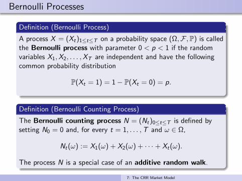
Definition (Bernoulli Process)
A process X = (Xt)1≤t≤T on a probability space (Ω,F ,P) is calledthe Bernoulli process with parameter 0 < p < 1 if the randomvariables X1,X2, . . . ,XT are independent and have the followingcommon probability distribution
P(Xt = 1) = 1− P(Xt = 0) = p.
Definition (Bernoulli Counting Process)
The Bernoulli counting process N = (Nt)0≤t≤T is defined bysetting N0 = 0 and, for every t = 1, . . . ,T and ω ∈ Ω,
Nt(ω) := X1(ω) + X2(ω) + · · · + Xt(ω).
The process N is a special case of an additive random walk.
7: The CRR Market Model
Stock Price
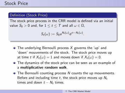
Definition (Stock Price)
The stock price process in the CRR model is defined via an initialvalue S0 > 0 and, for 1 ≤ t ≤ T and all ω ∈ Ω,
St(ω) := S0uNt(ω)d t−Nt(ω).
The underlying Bernoulli process X governs the ‘up’ and‘down’ mouvements of the stock. The stock price moves upat time t if Xt(ω) = 1 and moves down if Xt(ω) = 0.
The dynamics of the stock price can be seen as an example ofa multiplicative random walk.
The Bernoulli counting process N counts the up mouvements.Before and including time t, the stock price moves up Nt
times and down t − Nt times.
7: The CRR Market Model
Distribution of the Stock Price
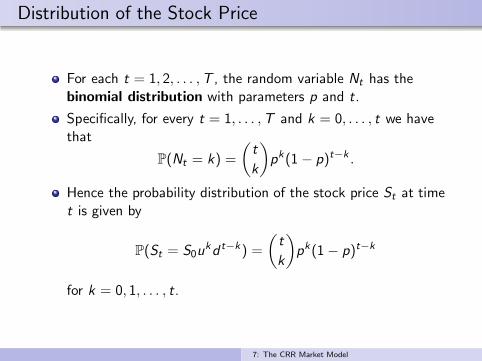
For each t = 1, 2, . . . ,T , the random variable Nt has thebinomial distribution with parameters p and t.
Specifically, for every t = 1, . . . ,T and k = 0, . . . , t we havethat
P(Nt = k) =
(t
k
)pk(1− p)t−k .
Hence the probability distribution of the stock price St at timet is given by
P(St = S0ukd t−k) =
(t
k
)pk(1− p)t−k
for k = 0, 1, . . . , t.
7: The CRR Market Model
Stock Price Lattice
−1
−0.8
−0.6
−0.4
−0.2
0
0.2
0.4
0.6
0.8
S0
S0u
S0d
S0u2
S0ud
S0d2
S0u3
S0u2d
S0d3
S0u4
S0u3d
S0u2d2
S0d4
S0ud2
S0ud3
...
...
...
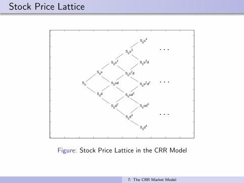
Figure: Stock Price Lattice in the CRR Model
7: The CRR Market Model
Risk-Neutral Probability Measure
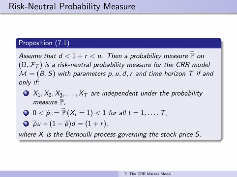
Proposition (7.1)
Assume that d < 1 + r < u. Then a probability measure P on
(Ω,FT ) is a risk-neutral probability measure for the CRR model
M = (B ,S) with parameters p, u, d , r and time horizon T if and
only if:
1 X1,X2,X3, . . . ,XT are independent under the probability
measure P,
2 0 < p := P (Xt = 1) < 1 for all t = 1, . . . ,T,
3 pu + (1− p)d = (1 + r),
where X is the Bernoulli process governing the stock price S.
7: The CRR Market Model
Risk-Neutral Probability Measure
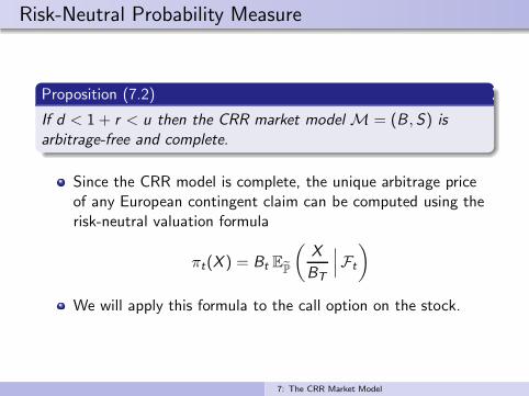
Proposition (7.2)
If d < 1 + r < u then the CRR market model M = (B ,S) isarbitrage-free and complete.
Since the CRR model is complete, the unique arbitrage priceof any European contingent claim can be computed using therisk-neutral valuation formula
πt(X ) = Bt EP
(X
BT
∣∣∣Ft
)
We will apply this formula to the call option on the stock.
7: The CRR Market Model
PART 2
THE CRR CALL OPTION PRICING FORMULA
7: The CRR Market Model
CRR Call Option Pricing Formula
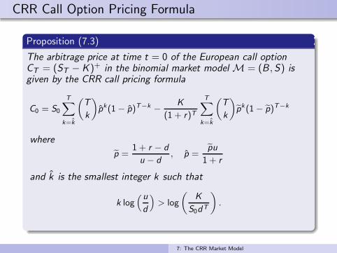
Proposition (7.3)
The arbitrage price at time t = 0 of the European call optionCT = (ST − K )+ in the binomial market model M = (B ,S) isgiven by the CRR call pricing formula
C0 = S0
T∑
k=k
(T
k
)pk(1− p)T−k − K
(1 + r)T
T∑
k=k
(T
k
)pk (1− p)T−k
where
p =1 + r − d
u − d, p =
pu
1 + r
and k is the smallest integer k such that
k log(ud
)> log
(K
S0dT
).
7: The CRR Market Model
Proof of Proposition 7.3
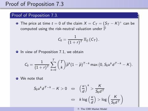
Proof of Proposition 7.3.
The price at time t = 0 of the claim X = CT = (ST − K )+ can be
computed using the risk-neutral valuation under P
C0 =1
(1 + r)TEP(CT ) .
In view of Proposition 7.1, we obtain
C0 =1
(1 + r)T
T∑
k=0
(T
k
)pk(1− p)T−k max
(0, S0u
kdT−k − K).
We note that
S0ukdT−k − K > 0 ⇔
(ud
)k
>K
S0dT
⇔ k log(ud
)> log
(K
S0dT
)
7: The CRR Market Model
Proof of Proposition 7.3
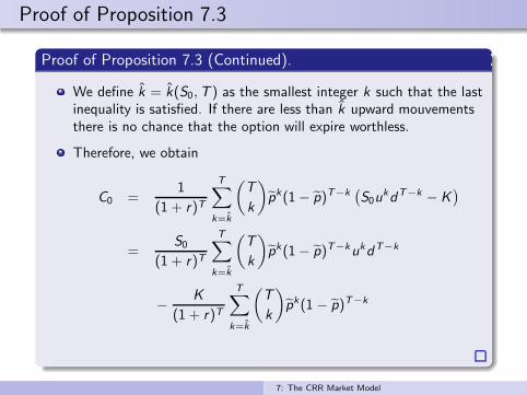
Proof of Proposition 7.3 (Continued).
We define k = k(S0,T ) as the smallest integer k such that the lastinequality is satisfied. If there are less than k upward mouvementsthere is no chance that the option will expire worthless.
Therefore, we obtain
C0 =1
(1 + r)T
T∑
k=k
(T
k
)pk(1− p)T−k
(S0u
kdT−k − K)
=S0
(1 + r)T
T∑
k=k
(T
k
)pk(1− p)T−kukdT−k
− K
(1 + r)T
T∑
k=k
(T
k
)pk(1 − p)T−k
7: The CRR Market Model

Proof of Proposition 7.3
Proof of Proposition 7.3 (Continued).
Consequently,
C0 = S0
T∑
k=k
(T
k
)(pu
1 + r
)k ((1 − p)d
1 + r
)T−k
− K
(1 + r)T
T∑
k=k
(T
k
)pk(1 − p)T−k
and thus
C0 = S0
T∑
k=k
(T
k
)pk(1− p)T−k − K
(1 + r)T
T∑
k=k
(T
k
)pk (1− p)T−k
where we denote p = pu1+r
.
7: The CRR Market Model
Martingale Approach (MATH3975)
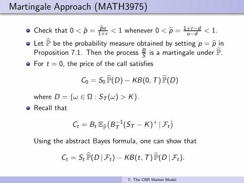
Check that 0 < p = pu1+r
< 1 whenever 0 < p = 1+r−du−d
< 1.
Let P be the probability measure obtained by setting p = p inProposition 7.1. Then the process B
Sis a martingale under P.
For t = 0, the price of the call satisfies
C0 = S0 P(D)− KB(0,T ) P(D)
where D = ω ∈ Ω : ST (ω) > K.Recall that
Ct = Bt EP
(B−1T (ST − K )+ | Ft
)
Using the abstract Bayes formula, one can show that
Ct = St P(D | Ft)− KB(t,T ) P(D | Ft).
7: The CRR Market Model
Put-Call Parity
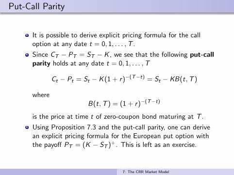
It is possible to derive explicit pricing formula for the calloption at any date t = 0, 1, . . . ,T .
Since CT − PT = ST − K , we see that the following put-callparity holds at any date t = 0, 1, . . . ,T
Ct − Pt = St − K (1 + r)−(T−t) = St − KB(t,T )
whereB(t,T ) = (1 + r)−(T−t)
is the price at time t of zero-coupon bond maturing at T .
Using Proposition 7.3 and the put-call parity, one can derivean explicit pricing formula for the European put option withthe payoff PT = (K − ST )
+. This is left as an exercise.
7: The CRR Market Model

PART 3
CALL AND PUT OPTIONS OF AMERICAN STYLE
7: The CRR Market Model
American Options
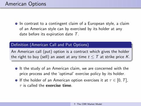
In contrast to a contingent claim of a European style, a claimof an American style can by exercised by its holder at anydate before its expiration date T .
Definition (American Call and Put Options)
An American call (put) option is a contract which gives the holderthe right to buy (sell) an asset at any time t ≤ T at strike price K .
It the study of an American claim, we are concerned with theprice process and the ‘optimal’ exercise policy by its holder.
If the holder of an American option exercises it at τ ∈ [0,T ],τ is called the exercise time.
7: The CRR Market Model
Stopping Times
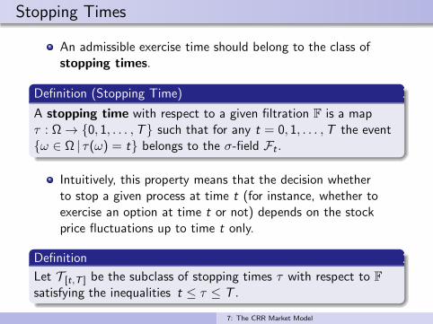
An admissible exercise time should belong to the class ofstopping times.
Definition (Stopping Time)
A stopping time with respect to a given filtration F is a mapτ : Ω → 0, 1, . . . ,T such that for any t = 0, 1, . . . ,T the eventω ∈ Ω | τ(ω) = t belongs to the σ-field Ft .
Intuitively, this property means that the decision whetherto stop a given process at time t (for instance, whether toexercise an option at time t or not) depends on the stockprice fluctuations up to time t only.
Definition
Let T [t,T ] be the subclass of stopping times τ with respect to F
satisfying the inequalities t ≤ τ ≤ T .
7: The CRR Market Model
American Call Option
Definition
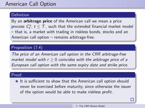
By an arbitrage price of the American call we mean a priceprocess C a
t , t ≤ T , such that the extended financial market model– that is, a market with trading in riskless bonds, stocks and anAmerican call option – remains arbitrage-free.
Proposition (7.4)
The price of an American call option in the CRR arbitrage-free
market model with r ≥ 0 coincides with the arbitrage price of a
European call option with the same expiry date and strike price.
Proof.
It is sufficient to show that the American call option shouldnever be exercised before maturity, since otherwise the issuerof the option would be able to make riskless profit.
7: The CRR Market Model
Proof of Proposition 7.4
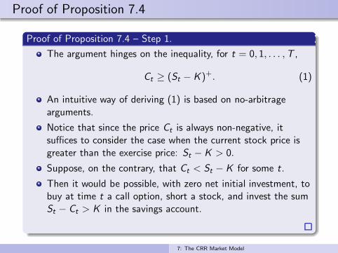
Proof of Proposition 7.4 – Step 1.
The argument hinges on the inequality, for t = 0, 1, . . . ,T ,
Ct ≥ (St − K )+. (1)
An intuitive way of deriving (1) is based on no-arbitragearguments.
Notice that since the price Ct is always non-negative, itsuffices to consider the case when the current stock price isgreater than the exercise price: St − K > 0.
Suppose, on the contrary, that Ct < St − K for some t.
Then it would be possible, with zero net initial investment, tobuy at time t a call option, short a stock, and invest the sumSt − Ct > K in the savings account.
7: The CRR Market Model
Proof of Proposition 7.4
Proof of Proposition 7.4 – Step 1.
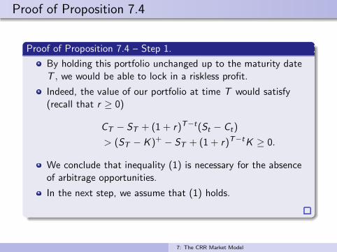
By holding this portfolio unchanged up to the maturity dateT , we would be able to lock in a riskless profit.
Indeed, the value of our portfolio at time T would satisfy(recall that r ≥ 0)
CT − ST + (1 + r)T−t(St − Ct)
> (ST − K )+ − ST + (1 + r)T−tK ≥ 0.
We conclude that inequality (1) is necessary for the absenceof arbitrage opportunities.
In the next step, we assume that (1) holds.
7: The CRR Market Model
Proof of Proposition 7.4
Proof of Proposition 7.4 – Step 2.
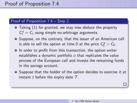
Taking (1) for granted, we may now deduce the propertyC at = Ct using simple no-arbitrage arguments.
Suppose, on the contrary, that the issuer of an American callis able to sell the option at time 0 at the price C a
0 > C0.
In order to profit from this transaction, the option writerestablishes a dynamic portfolio φ that replicates the valueprocess of the European call and invests the remaining fundsin the savings account.
Suppose that the holder of the option decides to exercise it atinstant t before the expiry date T .
7: The CRR Market Model
Proof of Proposition 7.4
Proof of Proposition 7.4 – Step 2.
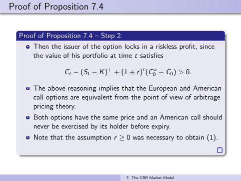
Then the issuer of the option locks in a riskless profit, sincethe value of his portfolio at time t satisfies
Ct − (St − K )+ + (1 + r)t(C a0 − C0) > 0.
The above reasoning implies that the European and Americancall options are equivalent from the point of view of arbitragepricing theory.
Both options have the same price and an American call shouldnever be exercised by its holder before expiry.
Note that the assumption r ≥ 0 was necessary to obtain (1).
7: The CRR Market Model
American Put Option
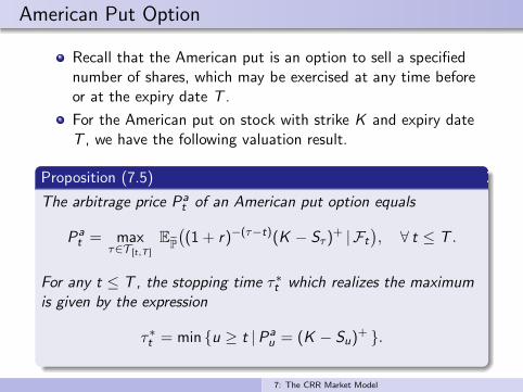
Recall that the American put is an option to sell a specifiednumber of shares, which may be exercised at any time beforeor at the expiry date T .
For the American put on stock with strike K and expiry dateT , we have the following valuation result.
Proposition (7.5)
The arbitrage price Pat of an American put option equals
Pat = max
τ∈T [t,T ]
EP
((1 + r)−(τ−t)(K − Sτ )
+ | Ft
), ∀ t ≤ T .
For any t ≤ T, the stopping time τ∗t which realizes the maximum
is given by the expression
τ∗t = min u ≥ t |Pau = (K − Su)
+ .
7: The CRR Market Model
PART 4
DYNAMIC PROGRAMMING APPROACH
TO AMERICAN CLAIMS
7: The CRR Market Model
Dynamic Programming Recursion
The stopping time τ∗t is called the rational exercise timeof an American put option that is assumed to be still aliveat time t.
By an application of the classic Bellman principle (1952),one reduces the optimal stopping problem in Proposition 7.5to an explicit recursive procedure for the value process.
The following corollary to Proposition 7.5 gives the dynamicprogramming recursion for the value of an American putoption.
Note that this is an extension of the backward inductionapproach to the valuation of European contingent claims.
7: The CRR Market Model
Dynamic Programming Recursion
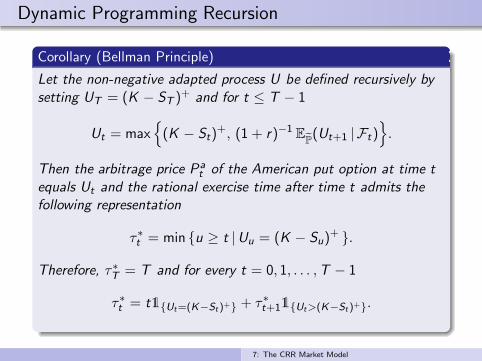
Corollary (Bellman Principle)
Let the non-negative adapted process U be defined recursively by
setting UT = (K − ST )+ and for t ≤ T − 1
Ut = max(K − St)
+, (1 + r)−1EP(Ut+1 | Ft)
.
Then the arbitrage price Pat of the American put option at time t
equals Ut and the rational exercise time after time t admits the
following representation
τ∗t = min u ≥ t |Uu = (K − Su)+ .
Therefore, τ∗T = T and for every t = 0, 1, . . . ,T − 1
τ∗t = t1Ut=(K−St)+ + τ∗t+11Ut>(K−St)+.
7: The CRR Market Model
Dynamic Programming Recursion
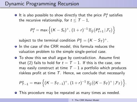
It is also possible to show directly that the price Pat satisfies
the recursive relationship, for t ≤ T − 1,
Pat = max
(K − St)
+, (1 + r)−1EP
(Pat+1 | Ft
)
subject to the terminal condition PaT = (K − ST )
+.
In the case of the CRR model, this formula reduces thevaluation problem to the simple single-period case.
To show this we shall argue by contradiction. Assume firstthat (2) fails to hold for t = T − 1. If this is the case, onemay easily construct at time T − 1 a portfolio which producesriskless profit at time T . Hence, we conclude that necessarily
PaT−1 = max
(K − ST−1)
+, (1+ r)−1EP
((K − ST )
+ | FT
).
This procedure may be repeated as many times as needed.
7: The CRR Market Model
American Put Option: Summary
To summarise:
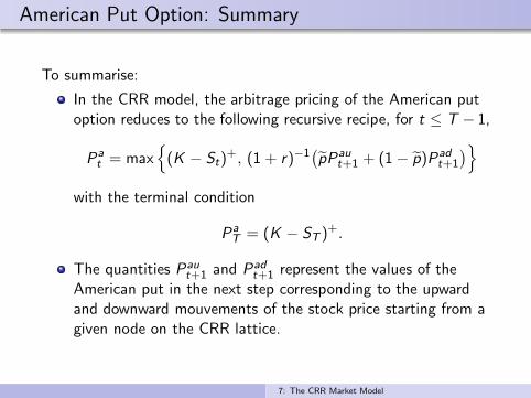
In the CRR model, the arbitrage pricing of the American putoption reduces to the following recursive recipe, for t ≤ T − 1,
Pat = max
(K − St)
+, (1 + r)−1(pPau
t+1 + (1− p)Padt+1
)
with the terminal condition
PaT = (K − ST )
+.
The quantities Paut+1 and Pad
t+1 represent the values of theAmerican put in the next step corresponding to the upwardand downward mouvements of the stock price starting from agiven node on the CRR lattice.
7: The CRR Market Model
General American Claim
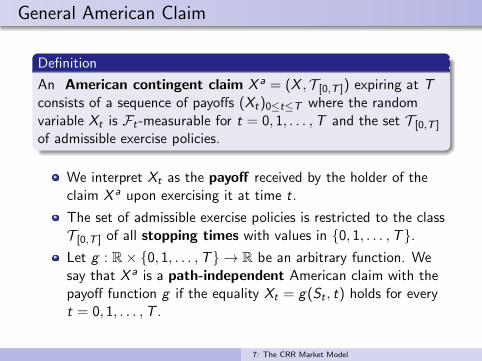
Definition
An American contingent claim X a = (X ,T [0,T ]) expiring at Tconsists of a sequence of payoffs (Xt)0≤t≤T where the randomvariable Xt is Ft -measurable for t = 0, 1, . . . ,T and the set T [0,T ]
of admissible exercise policies.
We interpret Xt as the payoff received by the holder of theclaim X a upon exercising it at time t.
The set of admissible exercise policies is restricted to the classT [0,T ] of all stopping times with values in 0, 1, . . . ,T.Let g : R× 0, 1, . . . ,T → R be an arbitrary function. Wesay that X a is a path-independent American claim with thepayoff function g if the equality Xt = g(St , t) holds for everyt = 0, 1, . . . ,T .
7: The CRR Market Model

General American Claim (MATH3975)
Proposition (7.6)
For every t ≤ T, the arbitrage price π(X a) of an American claim
X a in the CRR model equals
πt(Xa) = max
τ∈T [t,T ]
EP
((1 + r)−(τ−t)Xτ | Ft
).
The price process π(X a) satisfies the following recurrence relation,
for t ≤ T − 1,
πt(Xa) = max
Xt , EP
((1 + r)−1πt+1(X
a) | Ft
)
with πT (Xa) = XT and the rational exercise time τ∗t equals
τ∗t = minu ≥ t |Xu ≥ E
P
((1 + r)−1πu+1(X
a) | Fu
).
7: The CRR Market Model
Path-Independent American Claim: Valuation
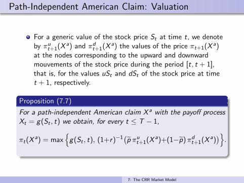
For a generic value of the stock price St at time t, we denoteby πu
t+1(Xa) and πd
t+1(Xa) the values of the price πt+1(X
a)at the nodes corresponding to the upward and downwardmouvements of the stock price during the period [t, t + 1],that is, for the values uSt and dSt of the stock price at timet + 1, respectively.
Proposition (7.7)
For a path-independent American claim X a with the payoff process
Xt = g(St , t) we obtain, for every t ≤ T − 1,
πt(Xa) = max
g(St , t), (1+r)−1
(p πu
t+1(Xa)+(1−p)πd
t+1(Xa))
.
7: The CRR Market Model
Path-Independent American Claim: Summary
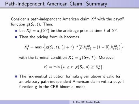
Consider a path-independent American claim X a with the payofffunction g(St , t). Then:
Let X at = πt(X
a) be the arbitrage price at time t of X a.
Then the pricing formula becomes
X at = max
g(St , t), (1 + r)−1
(p X au
t+1 + (1− p)X adt+1
)
with the terminal condition X aT = g(ST ,T ). Moreover
τ∗t = minu ≥ t | g(Su , u) ≥ X a
u
.
The risk-neutral valuation formula given above is valid foran arbitrary path-independent American claim with a payofffunction g in the CRR binomial model.
7: The CRR Market Model

Example: American Call Option
Example (7.1)
We consider here the CRR binomial model with the horizondate T = 2 and the risk-free rate r = 0.2.
The stock price S for t = 0 and t = 1 equals
S0 = 10, Su1 = 13.2, Sd
1 = 10.8.
Let X a be the American call option with maturity date T = 2and the following payoff process
g(St , t) = (St − Kt)+.
The strike Kt is variable and satisfies
K0 = 9, K1 = 9.9, K2 = 12.
7: The CRR Market Model
Example: American Call Option
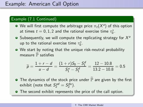
Example (7.1 Continued)
We will first compute the arbitrage price πt(Xa) of this option
at times t = 0, 1, 2 and the rational exercise time τ∗0 .
Subsequently, we will compute the replicating strategy for X a
up to the rational exercise time τ∗0 .
We start by noting that the unique risk-neutral probabilitymeasure P satisfies
p =1 + r − d
u − d=
(1 + r)S0 − Sd1
Su1 − Sd
1
=12− 10.8
13.2 − 10.8= 0.5
The dynamics of the stock price under P are given by the firstexhibit (note that Sud
2 = Sdu2 ).
The second exhibit represents the price of the call option.
7: The CRR Market Model
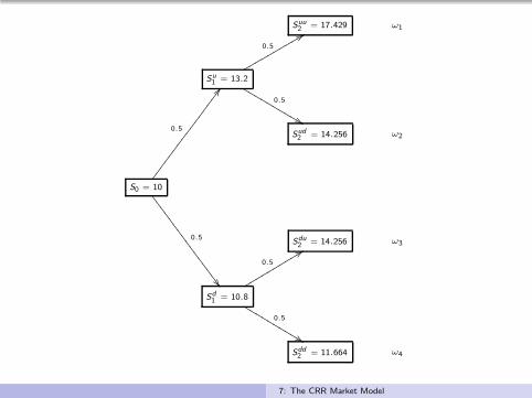
Suu2 = 17.429 ω1
Su1 = 13.2
0.5
88rrrrrrrrrr
0.5
&&LLL
LLLL
LLL
Sud2 = 14.256 ω2
S0 = 10
0.5
CC
0.5
777
7777
7777
7777
7
Sdu2 = 14.256 ω3
Sd1 = 10.8
0.5
99rrrrrrrrrr
0.5
%%LLL
LLLL
LLL
Sdd2 = 11.664 ω4
7: The CRR Market Model
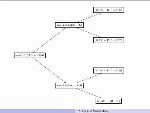
(17.429 − 12)+ = 5.429
max (3.3, 3.202) = 3.3
55kkkkkkkkkkkkkk
))SSSSS
SSSSSS
SSS
(14.256 − 12)+ = 2.256
max (1, 1.7667) = 1.7667
;;wwwwwwwwwwwwwwwwwwwww
##GGG
GGGG
GGGG
GGGG
GGGG
GG
(14.256 − 12)+ = 2.256
max (0.9, 0.94) = 0.94
55kkkkkkkkkkkkkk
))SSSSS
SSSSSS
SSS
(11.664 − 12)+ = 0
7: The CRR Market Model

Example: Replicating Strategy
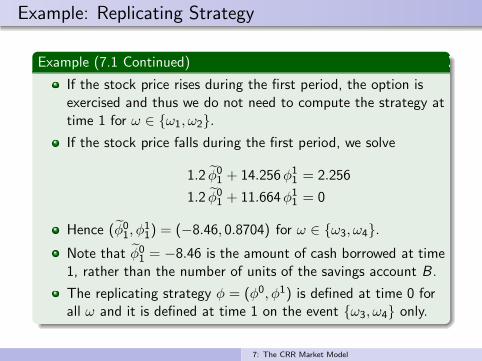
Example (7.1 Continued)
Holder. The rational holder should exercise the Americanoption at time t = 1 if the stock price rises during the firstperiod. Otherwise, the option should be held till time 2.Hence τ∗0 : Ω → 0, 1, 2 equals
τ∗0 (ω) = 1 for ω ∈ ω1, ω2τ∗0 (ω) = 2 for ω ∈ ω3, ω4
Issuer. We now take the position of the issuer of the option.At t = 0, we need to solve
1.2φ00 + 13.2φ1
0 = 3.3
1.2φ00 + 10.8φ1
0 = 0.94
Hence (φ00, φ
10) = (−8.067, 0.983) for all ω.
7: The CRR Market Model
Example: Replicating Strategy
Example (7.1 Continued)
If the stock price rises during the first period, the option isexercised and thus we do not need to compute the strategy attime 1 for ω ∈ ω1, ω2.If the stock price falls during the first period, we solve
1.2 φ01 + 14.256φ1
1 = 2.256
1.2 φ01 + 11.664φ1
1 = 0
Hence (φ01, φ
11) = (−8.46, 0.8704) for ω ∈ ω3, ω4.
Note that φ01 = −8.46 is the amount of cash borrowed at time
1, rather than the number of units of the savings account B .
The replicating strategy φ = (φ0, φ1) is defined at time 0 forall ω and it is defined at time 1 on the event ω3, ω4 only.
7: The CRR Market Model

− − −
V u1 (φ) = 3.3
55llllllllllllll
))RRRRR
RRRRRR
RRR
− − −
(φ00, φ
10) = (−8.067, 0.983)
::ttttttttttttttttttttt
$$HHH
HHHH
HHHH
HHHH
HHHH
HHH
V du2 (φ) = 2.256
(φ01, φ
11) = (−8.46, 0.8704)
66lllllllllllll
((RRRRR
RRRRRR
RR
V dd2 (φ) = 0
7: The CRR Market Model
PART 5
IMPLEMENTATION OF THE CRR MODEL
7: The CRR Market Model
Derivation of u and d from r and σ
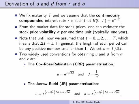
We fix maturity T and we assume that the continuouslycompounded interest rate r is such that B(0,T ) = e−rT .
From the market data for stock prices, one can estimate thestock price volatility σ per one time unit (typically, one year).
Note that until now we assumed that t = 0, 1, 2, . . . ,T , whichmeans that ∆t = 1. In general, the length of each period canbe any positive number smaller than 1. We set n = T/∆t.
Two widely used conventions for obtaining u and d from σand r are:
The Cox-Ross-Rubinstein (CRR) parametrisation:
u = eσ√
∆t and d =1
u.
The Jarrow-Rudd (JR) parameterisation:
u = e
(r− σ
2
2
)∆t +σ
√
∆tand d = e
(r− σ
2
2
)∆t − σ
√
∆t.
7: The CRR Market Model
The CRR parameterisation
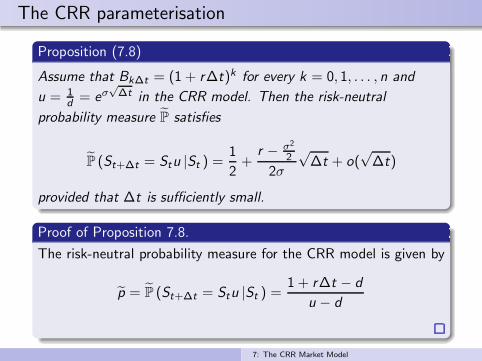
Proposition (7.8)
Assume that Bk∆t = (1 + r∆t)k for every k = 0, 1, . . . , n and
u = 1d= eσ
√∆t in the CRR model. Then the risk-neutral
probability measure P satisfies
P (St+∆t = Stu |St ) =1
2+
r − σ2
2
2σ
√∆t + o(
√∆t)
provided that ∆t is sufficiently small.
Proof of Proposition 7.8.
The risk-neutral probability measure for the CRR model is given by
p = P (St+∆t = Stu |St ) =1 + r∆t − d
u − d
7: The CRR Market Model
The CRR parameterisation
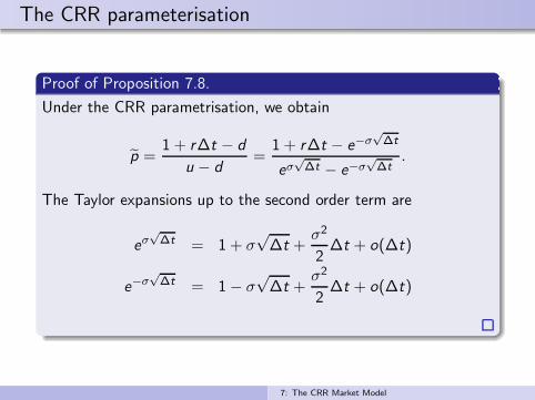
Proof of Proposition 7.8.
Under the CRR parametrisation, we obtain
p =1 + r∆t − d
u − d=
1 + r∆t − e−σ√∆t
eσ√∆t − e−σ
√∆t
.
The Taylor expansions up to the second order term are
eσ√∆t = 1 + σ
√∆t +
σ2
2∆t + o(∆t)
e−σ√∆t = 1− σ
√∆t +
σ2
2∆t + o(∆t)
7: The CRR Market Model
The CRR parameterisation
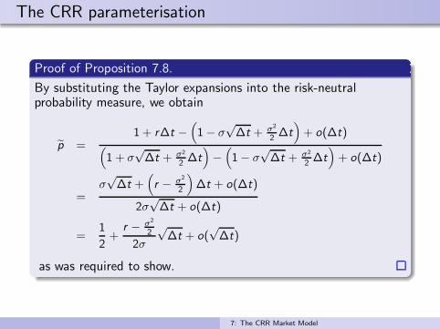
Proof of Proposition 7.8.
By substituting the Taylor expansions into the risk-neutralprobability measure, we obtain
p =1 + r∆t −
(1− σ
√∆t + σ
2
2 ∆t)+ o(∆t)
(1 + σ
√∆t + σ
2
2 ∆t)−(1− σ
√∆t + σ
2
2 ∆t)+ o(∆t)
=σ√∆t +
(r − σ
2
2
)∆t + o(∆t)
2σ√∆t + o(∆t)
=1
2+
r − σ2
2
2σ
√∆t + o(
√∆t)
as was required to show.
7: The CRR Market Model
The CRR parameterisation
To summarise, for ∆t sufficiently small, we get
p =1 + r∆t − e−σ
√∆t
eσ√∆t − e−σ
√∆t
≈ 1
2+
r − σ2
2
2σ
√∆t.
Note that 1 + r∆t ≈ er∆t when ∆t is sufficiently small.
Hence the risk-neutral probability measure can also berepresented as follows
p ≈ er∆t − e−σ√∆t
eσ√∆t − e−σ
√∆t
.
More formally, if we define r such that (1 + r)n = erT for afixed T and n = T/∆t then r ≈ r∆t since ln(1 + r) = r∆t
and ln(1 + r) ≈ r when r is close to zero.
7: The CRR Market Model

Example: American Put Option
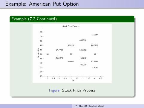
Example (7.2 – CRR Parameterisation)
Let the annualized variance of logarithmic returns be σ2 = 0.1.
The interest rate is set to r = 0.1 per annum.
Suppose that the current stock price is S0 = 50.
We examine European and American put options with strikeprice K = 53 and maturity T = 4 months (i.e. T = 1
3).
The length of each period is ∆t = 112 , that is, one month.
Hence n = T∆t
= 4 steps.
We adopt the CRR parameterisation to derive the stock price.
Then u = 1.0956 and d = 1/u = 0.9128.
We compute 1 + r∆t = 1.00833 ≈ er∆t and p = 0.5228.
7: The CRR Market Model
Example: American Put Option
Example (7.2 Continued)
0 0.5 1 1.5 2 2.5 3 3.5 4 4.525
30
35
40
45
50
55
60
65
70
75
50
54.7792
45.6378
60.0152
50
41.6561
65.7516
54.7792
45.6378
38.0219
72.0364
60.0152
50
41.6561
34.7047
t/∆ t
Sto
ck P
rice
Stock Price Process
Figure: Stock Price Process
7: The CRR Market Model
Example: American Put Option
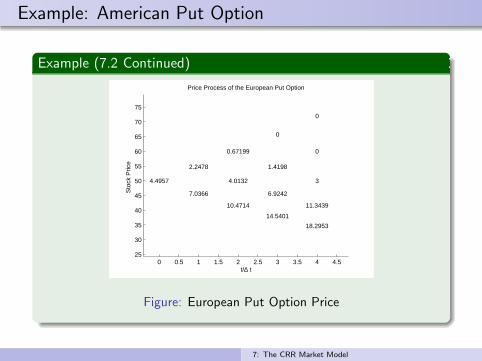
Example (7.2 Continued)
0 0.5 1 1.5 2 2.5 3 3.5 4 4.525
30
35
40
45
50
55
60
65
70
750
0
3
11.3439
18.2953
0
1.4198
6.9242
14.5401
0.67199
4.0132
10.4714
2.2478
7.0366
4.4957
t/∆ t
Sto
ck P
rice
Price Process of the European Put Option
Figure: European Put Option Price
7: The CRR Market Model

Example: American Put Option
Example (7.2 Continued)
0 0.5 1 1.5 2 2.5 3 3.5 4 4.525
30
35
40
45
50
55
60
65
70
750
0
3
11.3439
18.2953
0
1.4198
7.3622
14.9781
0.67199
4.2205
11.3439
2.3459
7.557
4.7928
t/∆ t
Sto
ck P
rice
Price Process of the American Put Option
Figure: American Put Option Price
7: The CRR Market Model
Example: American Put Option
Example (7.2 Continued)
0 0.5 1 1.5 2 2.5 3 3.5 4 4.5
30
40
50
60
70
80
1
1
1
1
1
1
0
1
1
0
0
1
0
0
0
t/∆ t
Sto
ck P
rice
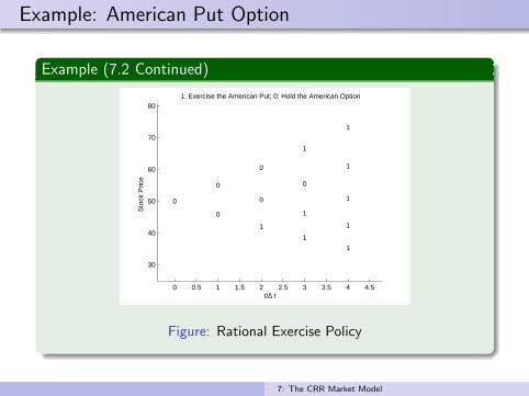
1: Exercise the American Put; 0: Hold the American Option
Figure: Rational Exercise Policy
7: The CRR Market Model
The JR parameterisation
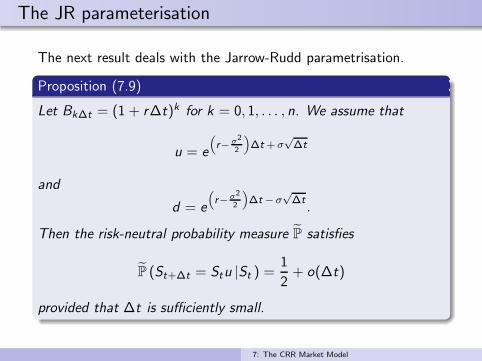
The next result deals with the Jarrow-Rudd parametrisation.
Proposition (7.9)
Let Bk∆t = (1 + r∆t)k for k = 0, 1, . . . , n. We assume that
u = e
(r−σ2
2
)∆t + σ
√∆t
and
d = e
(r−σ2
2
)∆t − σ
√∆t
.
Then the risk-neutral probability measure P satisfies
P (St+∆t = Stu |St ) =1
2+ o(∆t)
provided that ∆t is sufficiently small.
7: The CRR Market Model

The JR parameterisation
Proof of Proposition 7.9.
Under the JR parametrisation, we have
p =1 + r∆t − d
u − d=
1 + r∆t − e
(r−σ2
2
)∆t−σ
√∆t
e
(r−σ2
2
)∆t+σ
√∆t − e
(r−σ2
2
)∆t−σ
√∆t
.
The Taylor expansions up to the second order term are
e
(r−σ2
2
)∆t+σ
√∆t
= 1 + r∆t + σ√∆t + o(∆t)
e
(r−σ2
2
)∆t−σ
√∆t
= 1 + r∆t − σ√∆t + o(∆t)
and thus
p =1
2+ o(∆t).
7: The CRR Market Model
Example: American Put Option
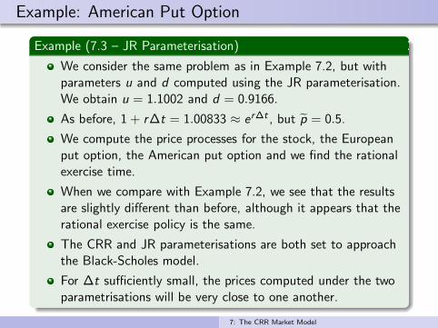
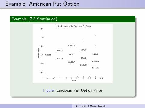
Example (7.3 – JR Parameterisation)
We consider the same problem as in Example 7.2, but withparameters u and d computed using the JR parameterisation.We obtain u = 1.1002 and d = 0.9166.
As before, 1 + r∆t = 1.00833 ≈ er∆t , but p = 0.5.
We compute the price processes for the stock, the Europeanput option, the American put option and we find the rationalexercise time.
When we compare with Example 7.2, we see that the resultsare slightly different than before, although it appears that therational exercise policy is the same.
The CRR and JR parameterisations are both set to approachthe Black-Scholes model.
For ∆t sufficiently small, the prices computed under the twoparametrisations will be very close to one another.
7: The CRR Market Model
Example: American Put Option
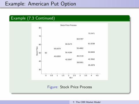
Example (7.3 Continued)
0 0.5 1 1.5 2 2.5 3 3.5 4 4.5
30
40
50
60
70
80
50
55.0079
45.8283
60.5174
50.4184
42.0047
66.5787
55.4682
46.2118
38.5001
73.2471
61.0238
50.8403
42.3562
35.2879
t/∆ t
Sto
ck P
rice
Stock Price Process
Figure: Stock Price Process
7: The CRR Market Model
Example: American Put Option
Example (7.3 Continued)
0 0.5 1 1.5 2 2.5 3 3.5 4 4.5
30
40
50
60
70
80
0
0
2.1597
10.6438
17.7121
0
1.0709
6.3488
14.0607
0.53103
3.6792
10.1204
2.0877
6.8428
4.4284
t/∆ t
Sto
ck P
rice
Price Process of the European Put Option
Figure: European Put Option Price
7: The CRR Market Model
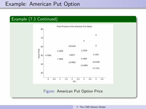
Example: American Put Option
Example (7.3 Continued)
0 0.5 1 1.5 2 2.5 3 3.5 4 4.5
30
40
50
60
70
80
0
0
2.1597
10.6438
17.7121
0
1.0709
6.7882
14.4999
0.53103
3.8971
10.9953
2.1958
7.3846
4.7506
t/∆ t
Sto
ck P
rice
Price Process of the American Put Option
Figure: American Put Option Price
7: The CRR Market Model

Example: American Put Option
Example (7.3 Continued)
0 0.5 1 1.5 2 2.5 3 3.5 4 4.5
30
40
50
60
70
80
1
1
1
1
1
1
0
1
1
0
0
1
0
0
0
t/∆ t
Sto
ck P
rice
1: Exercise the American Put; 0: Hold the American Option
Figure: Rational Exercise Policy
7: The CRR Market Model


![A Skewness-Adjusted Binomial Model for Pricing …file.scirp.org/pdf/JMF20120100011_82298793.pdf · Black-Scholes (B-S) [2] model and the binomial option pricing model (BOPM) with](https://img.dokumen.tips/doc/110x75/5b6b45f97f8b9a422e8d3f09/a-skewness-adjusted-binomial-model-for-pricing-filescirporgpdfjmf20120100011.jpg)